Security Proofs for Quantum Key Distribution Protocols by Numerical Approaches by Jie Lin A thesis presented to the University of Waterloo in fulfillment of the thesis requirement for the degree of Master of Science in Physics (Quantum Information) Waterloo, Ontario, Canada, 2017 c Jie Lin 2017
Transcript
Security Proofs for Quantum Key Distribution
Protocols by Numerical Approaches
by
Jie Lin
A thesispresented to the University of Waterloo
in fulfillment of thethesis requirement for the degree of
I hereby declare that I am the sole author of this thesis. This is a true copy of the thesis,including any required final revisions, as accepted by my examiners.
I understand that my thesis may be made electronically available to the public.
Jie Lin
ii
Abstract
This thesis applies numerical methods to analyze the security of quantum key distribution(QKD) protocols. The main theoretical problem in QKD security proofs is to calculate thesecret key generation rate. Under certain assumptions, this problem has been formulatedas a convex optimization problem and numerical methods [8, 41] have been proposed toproduce reliable lower bounds for discrete-variable QKD protocols. We investigate theapplicability of these numerical approaches and apply the numerical methods to study avariety of protocols, including measurement-device-independent (MDI) protocols, varia-tions of the BB84 protocol with a passive countermeasure against Trojan horse attacks,and the phase-encoding BB84 protocol using attenuated laser sources without continuousphase randomization.
iii
Acknowledgements
First of all, I would like to thank my supervisor Norbert Lutkenhaus who gave me theopportunity to pursue my Master of Science study in the Institute for Quantum Computing.I want to thank him for his support, helpful discussion and advices in the past two years.
Thanks to my colleagues in the OQCT research group and many members of IQC. Ihave learned so much from all of them. In particular, I would like to give my special thankto Patrick Coles for helpful discussion about the numerical approaches, both the dualproblem approach and the primal problem approach. I would also like to thank AdamWinick for enlightening discussion about the primal problem approach, and choices ofoptimization algorithms. Without the help from them, I cannot complete the calculationsfor this thesis. I would also like to thank Yanbao Zhang, Michael Epping, Hao Qin andPoompong Chaiwongkhot for proofreading early versions of this thesis.
I also want to thank Steve Weiss for his technical support and arrangement of IQCHeavylift computers.
I would like to thank all my friends here at Waterloo. Thanks to Ace and Golson forbeing wonderful roommates and friends and for sharing a lot of helpful tips about Waterloo.
Finally, I would like to thank my family for their love, support and encouragement.
3.1 A table for this MDI QKD protocol with BB84 signal states, showing therelation between the state in Alice’s (Bob’s) register A (B) and the signalstate prepared as well as the basis choice and bit value after applying a keymap. . . . . . . . . . . . . . . . . . . . . . . . . . . . . . . . . . . . . . . 40
3.2 The list of situations that would lead to an error, conditioning on thatCharlie announces the measurement outcome corresponding to |Φ+〉 . Thefirst row lists the state of AB after measurements of Alice and Bob. Thesecond row lists the corresponding states they prepare for Charlie. Theinterpretation of these states is listed in Table 3.1. . . . . . . . . . . . . . 42
4.1 Parameters used in the data simulation for the key rate calculation in thecase of Trojan horse attacks. Those parameters are taken from Ref. [25]. . 65
4.2 Signal states and a priori probability distribution for the phase-randomizedlaser source. By using the idea of tagging, we can think that the sourceemits one of these nine states. pµ0 is the probability of emitting vacuumstate from a Poisson distribution with mean photon number µ. Similarly,pµ1 is the probability of emitting single photons, and pµmulti for multi-photons. 70
4.3 Source-replacement states for phase-randomized laser source. By using theidea of tagging, we can think the source emits one of these 12 states. Themeaning of probabilities is the same as in Table 4.2. Since multi-photonstates are orthogonal to each other, there is no need to attach Trojan horsepulses because Eve has complete knowledge. . . . . . . . . . . . . . . . . . 70
5.1 Simulation parameters for this BB84 protocol with phase-encoding using aphase-coherent laser source. . . . . . . . . . . . . . . . . . . . . . . . . . . 76
viii
List of Figures
2.1 Schematics of squashing model, reproduced from the Fig. 1 of Ref. [13]. Inreality, the measurement device may perform the POVM FB. By applyingan appropriate post-processing, the full measurement is now described byPOVM FM . If there exists a squashing map, then it allows us to think themeasurement in terms of the target POVM FQ on a lower-dimensional space. 14
2.2 Schematic description of entropy. The left circle represents the amount ofcertainty for X, and the right circle represents the amount of uncertaintyfor Y . The blue area represents H(X|Y ); green area H(Y |X) and grey areaI(X : Y ). . . . . . . . . . . . . . . . . . . . . . . . . . . . . . . . . . . . . 16
3.1 Schematic description of MDI protocols. Alice and Bob both prepare signalstates and send to an untrusted third party Charlie. Charlie performs a jointmeasurement on both signals in a black box (from Alice and Bob’s perspec-tive) and publicly announces the measurement outcomes. In this setup, Evecan control both quantum channels and Charlie, as well as listening to thecommunication in the classical channel. . . . . . . . . . . . . . . . . . . . 38
3.2 Key rate for MDI protocol with BB84 signal states using a single-photonsource. This plot shows the asymptotic key rate of MDI BB84 as a functionof the observed error rate Q. Blue solid dots are our numerical results usingthe dual problem approach described in Theorem 3.5, and black dashed lineis the theoretical key rate, which is 1− 2h(Q) in this case. . . . . . . . . . 42
3.3 Key rate for MDI protocol with B92 signal states |+α〉 and |−α〉. This plotshows the asymptotic key rate of MDI B92 as a function of the amplitudeof the coherent state. Blue solid dots are our numerical results using thedual problem approach described in Theorem 3.5, and black dashed line isthe analytically calculated key rate in Ref. [10]. . . . . . . . . . . . . . . . 45
ix
3.4 Illustration of the numerical method in a 1-dimensional abstraction. Thegap between our lower bound and the optimal value can be made smallerby finding ρ closer to the optimal ρ∗. Red arrows indicate the optimizationswe actually perform. . . . . . . . . . . . . . . . . . . . . . . . . . . . . . . 47
3.5 Key rate as a function of observed error rate Q for single-photon BB84with single-photon transmission probability η = 1. The solid dots are ournumerical results using the primal problem approach and the lines are givenby the analytical key rate expression R∞BB84 = (p2
z + (1 − pz)2)(1 − 2h(Q)).Different curves correspond to different a priori probabilities for basis choice.This is a demonstration of handling sifting in the numerical framework. . 54
3.6 Key rate as a function of observed error rate Q for single-photon BB84with single-photon transmission probability η = 0.8. The solid dots are ournumerical results using the primal problem approach and the lines are givenby the analytical key rate expression R∞BB84,loss = η(p2
4.1 Schematics of Trojan horse attacks on Alice’s devices. Eve injects a coherentlight into Alice’s system to probe the encoding device’s setting. Some partof the light is reflected back to carry the information about the secret infor-mation. By measuring the back-reflected lights, Eve can break the securityof QKD. . . . . . . . . . . . . . . . . . . . . . . . . . . . . . . . . . . . . . 59
4.2 Asymptotic key rate versus the intensity of back-reflected Trojan horse lightµout for different observed error rates. Solid dots are our numerical resultsand lines are given by Eq. (4.3). Parameters are listed in the figure. Weconsider ideal parameters for simplicity. We numerically observe the keyrate is a convex function of µout. . . . . . . . . . . . . . . . . . . . . . . . . 64
4.3 Asymptotic key rate versus the transmission distance for various intensitiesof back-reflected Trojan horse light µout. Solid dots are our numerical resultsand lines are given by Eq. (4.3). Parameters are listed in the Table 4.1. . 66
x
4.4 Asymptotic key rate versus the transmission distance for various intensitiesof Alice’s signal intensity µ. η = 12.5%. Blue diamond curve represents thekey rate in the situation if we assume Trojan horse photons are completelyblocked. Black circle curve represents the key rate in the case the Trojanhorse photons are of intensity µout = 10−3. The connected line representsthe calculation if we assume Trojan horse photons are completely blocked,but the intensity of lights coming out from Alice’s laboratory is actuallyµ + µout = µ + 10−3 and the transmission probability is actually η µ
µ+µout.
Other parameters are listed in the Table 4.1. . . . . . . . . . . . . . . . . 68
4.5 The asymptotic key rate versus the transmission distance for a phase-randomizedcoherent state source for different intensities of back-reflected lights µout.Solid dots are our numerical results. . . . . . . . . . . . . . . . . . . . . . . 72
5.1 Schematics of the phase-encoding BB84 protocol: the attenuated laser sourceemits a coherent state, which is split by the 50/50 beam splitter (BS) intoa reference pulse and a signal pulse. A phase modulator (PM) is used toencode the information about the secret key in the signal pulse. Both thesignal pulse and the reference pulse are transmitted through the same fiberto Bob. One may use polarization rotators (PR) and polarizing beam split-ters (PBS) to pack the signal and reference pulses for transmission. (Or onecan apply adjustable time delay to the pulses such that they arrive at thesame time at the interferometer in Bob’s lab.) In Bob’s lab, he applies 0 orπ2
phase shift to the reference pulse via a phase modulator (PM). This allowshim to choose the measurement basis. The signal pulse and the referencepulse will then interfere at the 50/50 beam splitter and trigger one of thedetectors. . . . . . . . . . . . . . . . . . . . . . . . . . . . . . . . . . . . . 75
5.2 The asymptotic key rate versus the intensity µ of the signal pulse for thisphase-encoding BB84 protocol using phase-coherent laser source for differenttransmission probabilities η = 0.045 (L = 0 km) and η = 0.0357 (L = 5 km)for the parameters listed in Table 5.1. The phase information is assumed tobe known by Eve. Solid dots are our numerical results and lines are givenby the analytical expression in Ref. [24]. . . . . . . . . . . . . . . . . . . . 78
xi
5.3 The asymptotic key rate versus the intensity µ of the signal pulse for thisphase-encoding BB84 protocol using phase-coherent laser source for twovalues of total transmission probability η = 1 and η = 0.8. The phaseinformation is assumed to be known by Eve. Other simulation parameters,such as dark count rate, are ideal as described in the main text. Solid dotsare our numerical results and lines are given by the analytical expression inRef. [24]. . . . . . . . . . . . . . . . . . . . . . . . . . . . . . . . . . . . . . 79
5.4 The schematics of Alice’s device. Compared with Fig. 5.1, an additionalphase modulator (PM1) is inserted immediately after the source to random-ize the phase of coherent states. This phase modulator randomly appliesone of the N possible choices of phase to each coherent state before it issplit into a reference pulse and a signal pulse. . . . . . . . . . . . . . . . . 80
5.5 The asymptotic key rate versus the transmission distance in the case ofdiscrete phase randomization without decoy states. The key rate is plottedin the logarithmic scale. Solid dots are our numerical results in the caseN = 1, 2, 3, 4. We compare our numerical results with the results (lines)reported in Ref. [5]. Red curves and dots are for N = 1; yellow for N = 2;purple for N = 3 and green for N = 4. The blue dashed line is the key ratewith a continuous phase-randomized source. . . . . . . . . . . . . . . . . . 84
xii
Chapter 1
Introduction
Since the invention of first quantum key distribution (QKD) protocol BB84 by CharlesBennett and Gilles Brassard in 1984 [2], over the past three decades, this field has advanceddramatically both in theory and in physical implementation [33].
Unlike conventional cryptographic schemes whose security is based on computationalassumptions, QKD guarantees the security by the laws of quantum mechanics. In theory,QKD has been proven to be unconditionally secure [15, 18, 21, 28, 35]. However, thephysical implementation of QKD deviates from the theoretical model in many aspects andthe gap between implementation and theory is vulnerable to eavesdropping attacks. Toclose up the gap, from the theory side, the security proofs need to be modified by relaxingthe assumptions and taking into account what can be achieved by the current technology.Analytical security proofs can be quite complicated and the key rate bound can be loosedue to available proof techniques. On the other hand, the key rate calculation problem canbe formulated as a convex optimization problem and therefore we can resort to computersto perform the key rate calculation. In this thesis, we will apply numerical approachesdeveloped recently in Refs. [8, 41] to study various QKD protocols.
This thesis is organized as follows:
In chapter 2, we will review the basics of quantum mechanics, quantum key distribution,entropy, quantum optics and convex optimization.
In chapter 3, we will discuss the fundamental theoretical problem in QKD - the key rateproblem. We will start with reviewing the theoretical frameworks developed previously, inparticular, the universally composable security definition and general key rate formulas.Then we will discuss the particular key rate calculation problem we will focus on for this
1
thesis and how this problem has been formulated as a convex optimization problem. Thenwe will discuss the numerical security proof techniques developed recently. We have beenable to use a modified dual problem approach to tackle the key rate calculation of manyprotocols. We will briefly mention the advantages and disadvantages of this approach.We will also show some examples to illustrate how we treat each protocol in our numericalframework. Then we will discuss the primal problem approach and and the idea of obtaininga reliable lower bound from the primal problem. We end this chapter by discussing howwe handle sifting in the numerical framework, in particular, within the primal problemapproach.
In chapter 4, we will show the applications of the numerical approaches. In particular,we will consider the analysis of QKD protocols with some passive optical componentsacting as a countermeasure to the Trojan horse attacks. We will see how our numericalapproaches give a better key rate bound. Our analysis considers various types of sources,including a single-photon source, phase-coherent laser source and phase-randomized lasersource.
In chapter 5, we will apply numerical approaches to study phase-encoding BB84 pro-tocols with an attenuated laser source. We analyze the phase-coherent source where thephase is known by Eve. We will also investigate the idea of phase randomization andpresent our numerical security proofs in the case of discrete phase randomization.
In chapter 6, we make some concluding remarks and give the outlook for future works.
2
Chapter 2
Background
2.1 Quantum mechanics
In this section, we will review the basic formulation of quantum mechanics that is relevantfor understanding this thesis and also introduce some notations we will use. The sectionis mainly based on [31]. Readers can refer to it for details.
2.1.1 Quantum states
Given a physical system1 of interest, every (pure) quantum state, denoted by a ket vector|ψ〉, lives in a complex Hilbert space H, which we call the state space of this physicalsystem. We will use subscripts to label different systems when our discussion involvesmultiple systems. For each ket vector |ψ〉 ∈ H, its dual vector 〈ψ|, a bra vector, lives inthe dual space of H, which is isomorphic to itself.2 Then 〈φ|ψ〉 ∈ C denotes the innerproduct of two states |φ〉 , |ψ〉 ∈ H, and the outer product |φ〉〈ψ| is a linear map from Hto itself. In particular, |φ〉〈φ| is a projector onto the state vector |φ〉.
We may be interested in a bipartite system composed of two subsystems A and B withassociated state spaces HA and HB, respectively. The composite system of both A andB has the state space HAB = HA ⊗HB with dimHAB = dAdB, where dA = dimHA and
1In this thesis, we will also use the term register for the physical system of our interest. Formallyspeaking, a register is an abstraction of a physical device that stores quantum information.
2 Mathematically, a dual vector 〈ψ| is a linear functional from H to C, and the dual space is the spaceof all bounded linear functionals, each of which maps every vector from H to a complex number.
3
dA = dimHB. In this thesis, most of the time we will deal with finite-dimensional Hilbertspaces unless stated otherwise.3 If |i〉A
dAi=1 is a basis for HA and |j〉B
dBj=1 is a basis for
HB, then |i〉A⊗ |j〉BdA,dBi,j=1 is a basis for HAB. We sometimes write |i〉A⊗ |j〉B as |i〉A |j〉B
or |ij〉AB for the ease of notation. We will drop the subscripts when the spaces in ourdiscussion are clear.
The system can also be prepared in a statistical ensemble of pure states. In this case,such a state is called a mixed state and it cannot be described by a single ket vector. So,we resort to a more general mathematical description of the quantum states, that is, thedensity operator formulation. First, we define the density operators for pure states. Thedensity operator associated to the state vector |ψ〉 is ρ = |ψ〉〈ψ|. For a classical mixture ofpure states |ψi〉 with a probability distribution pi, the density operator is given by
ρ =∑i
pi |ψi〉〈ψi| . (2.1)
In a finite-dimensional Hilbert space, we can choose an orthonormal basis and thenwrite every density operator in the matrix form, called the density matrix. We will use thewords density operator and density matrix interchangeably.
We will also be interested in linear operators on H. We denote L(H) as the set ofall linear operators on H. In particular, we will be interested in Hermitian operators andpositive semi-definite operators. Here, we review the definitions of Hermitian operators,and positive semi-definite operators.
Definition 2.1. (Hermitian operator) A Hermitian operator X is a linear operator suchthat for every |ψ〉 ∈ H, 〈ψ|X |ψ〉 ∈ R. Equivalently, a linear operator X is Hermitian ifX = X†, where X† is its adjoint operator.4 We denote the set of Hermitian operators onH as Herm(H).
Definition 2.2. (Positive semidefinite operator) A positive semi-definite operator P is alinear operator such that for every |ψ〉 ∈ H, 〈ψ|P |ψ〉 ≥ 0. If P is positive semidefinite,we write P 0. The set of all positive semidefinite operators on H is denoted as Pos(H).
It is clear from the definition that a positive semidefinite operator is also a Hermitianoperator.
We now can give a general mathematical definition of density operators.
3Later, we will also discuss a particular infinite-dimensional Hilbert space, called Fock space.4The adjoint operator X† of X is defined as
⟨X†φ
∣∣ψ⟩ = 〈φ|Xψ〉, where |ψ〉 and |φ〉 are arbitrary statevectors.
4
Definition 2.3. (Density operator) A density operator ρ is a positive semidefinite operatorsuch that Tr(ρ) = 1. We denote the set of all density operators as D(H).
Because the density matrix ρ represents a state of the system and H is the state space,we will often say ρ in H even though formally ρ ∈ D(H).
Next, we discuss how to describe a subsystem. Suppose ρAB is the density operatorfor a bipartite system consisting of two subsystems A and B. If we are only interested inthe subsystem A, then we can describe this subsystem by the reduced density operatorρA = TrB(ρAB) after tracing out the system B. Similarly, we can describe the subsystemB by ρB.
If the joint state ρAB is pure, by the following theorem, we then know that ρA and ρBshare the same set of eigenvalues.
Theorem 2.4 (Schmidt decomposition). Let ρAB = |ψ〉〈ψ|AB be a pure state in HAB. Thenwe can write
|ψ〉AB =∑i
√λi |ei〉A |ei〉B , (2.2)
ρA := TrB(ρAB) =∑
i λi |ei〉〈ei|A, and ρB := TrA(ρAB) =∑
i λi |ei〉〈ei|B, where |ei〉A and|ei〉B are orthonormal sets on HA and HB, respectively.
In many scenarios, it is more convenient to deal with pure states than mixed states.The following theorem is helpful for converting an arbitrary mixed state in a smaller spaceto a pure state in a larger space.
Theorem 2.5 (Purification). Let ρA be a state in HA. Then there exists a reference spaceHR with dimHR = dimHA, and a pure state |ψ〉 ∈ HA ⊗HR such that ρA = TrR(|ψ〉〈ψ|).
Such a purification can be constructed as the following:
We start with the orthogonal decomposition of ρA =∑d
i=1 pi |i〉〈i|A , where |i〉Adi=1
is an orthonormal basis.5 Then we introduce a reference system R such that dimHR =dimHA = d and
∣∣i⟩Rdi=1 is an orthonormal basis for HR. We then define a pure state
|ψ〉 =∑d
i=1
√pi |i〉A
∣∣i⟩R. We notice that TrR(|ψ〉〈ψ|) =
∑di=1 pi |i〉〈i|A = ρA. Therefore,
|ψ〉 is a purification of ρA.
Finally, we end our discussion of quantum states with the definitions of separable states,entangled states and Bell states.
5Since ρA is also a Hermitian operator, such an orthogonal decomposition can be realized by its spectraldecomposition.
5
Definition 2.6. (Separable state) A state ρAB ∈ D(HAB) of some physical system AB isseparable if it can be written as a convex combination of product states:
ρAB =∑x
p(x)ρxA ⊗ ρxB.
Definition 2.7. (Entangled state) A state ρ ∈ D(H) is entangled if it is not separable.
Definition 2.8. (Bell states) The four Bell states are defined on a two-qubit Hilbert spaceas ∣∣Φ+
⟩=
1√2
(|00〉+ |11〉),∣∣Φ−⟩ =1√2
(|00〉 − |11〉),∣∣Ψ+⟩
=1√2
(|01〉+ |10〉),∣∣Ψ−⟩ =1√2
(|01〉 − |10〉).
(2.3)
These four Bell states are maximally entangled states.
2.1.2 Measurements
Every physical measurement can be described by a positive operator-valued measure (POVM),which is defined below.
Definition 2.9. (POVM) An n-outcome POVM on a Hilbert space H is a set Eini=1
such that Ei 0 for each i andn∑i=1
Ei = 1.
Also, every POVM can be realized by a physical measurement. Typically, one labelsthe outcomes of a measurement by the elements of the index set of its POVM. For aquantum state ρ ∈ D(H), and a physical measurement described by a POVM Fjmi=1, theprobability for the outcome j of the measurement to occur is given by Tr(ρFj).
A POVM Fj can be represented by a list of Kraus operators Mii∈I acting on the
Hilbert space H such that∑
i∈IM†iMi = 1 for some index set I, where 1 is the identity
operator. This representation is not unique and there can be several different lists of Krausoperators representing the same POVM. For a given list of Kraus operators, each POVM
6
element Fj can be written as Fj =∑
i∈Ij M†iMi, where the summation is over a subset Ij
of the index set I. For a quantum state ρ, the probability pk for the k-th outcome to occur
is given by pk =∑
i∈Ik Tr(ρM †
iMi
)and the post-measurement state conditioning on the
outcome k is∑i∈Ik
MiρM†i
pk.
A special type of measurements that we will frequently encounter is projective mea-surements or projection-valued measure (PVM), where each measurement operator is aprojection operator. A projection operator P is a positive semidefinite operator such thatP 2 = P = P †.
A general POVM is not necessarily a projective measurement. However, we can con-struct a projective measurement from a given POVM. This can be done through Naimarkdilation theorem. We state the Naimark dilation theorem in the form that is relevant toour discussion.
Theorem 2.10 (Naimark). Let Eini=1 be a POVM on HA. There exists a Hilbert spaceHR, an isometry V : HA → HA ⊗ HR and a projective measurement Pini=1 such thatEi = V †PiV for each i.
Here, we give an explicit construction of this isometry and the corresponding PVM.We first notice that for each positive semidefinite operator A, there exists a unique square-root operator B such that B2 = A. Since Ei is positive semidefinite, we write
√Ei as its
square-root operator. V can be constructed as V =∑
i
√Ei⊗ |i〉R. We verify that V is an
isometry since V †V =∑
iEi = 1A. Each element of the desired PVM can be constructedas Pi = 1A ⊗ |i〉〈i|R, which is a projection onto one of the basis states of the new registersystem R.
2.1.3 Quantum channel
To define a quantum channel, we start with the definitions of completely positive (CP)maps and trace-preserving (TP) maps.
Definition 2.11. A map Φ : L(HA)→ L(HB) is completely positive if for every complexEuclidean space Z, Φ ⊗ 1L(Z) is a positive map. Φ is trace-preserving if for every X ∈L(HA), Tr(Φ(X)) = Tr(X).
Definition 2.12. (Quantum channel) A quantum channel E between two registers A andB with HA and HB is a map from L(HA) to L(HB) such that it is completely positive andtrace-preserving (CPTP).
7
We notice that from the CPTP requirements, for ρ ∈ D(HA), we automatically haveE(ρ) ∈ D(HB).
An important representation of a quantum channel is its Kraus representation. A mapE from L(HA) to L(HB) is CP if and only if there exists a set of operators Ka suchthat E(X) =
∑a
KaXK†a for every X ∈ L(HA). It is trace-preserving (TP) if and only if∑
a
K†aKa = 1A. The operators Ka are called Kraus operators.
Before we end the discussion of quantum channels, we consider a particular channel ofa qubit system, called depolarizing channel. This is a model for introducing noise to thesystem.
Definition 2.13. (Depolarizing channel) For a qubit system, a depolarizing channel E :L(C2) → L(C2) is defined as E(ρ) = (1 − p)ρ + p1
2for every ρ ∈ L(C2), where p is the
depolarizing probability.
Since for arbitrary ρ, we have 12
= ρ+σxρσx+σyρσy+σzρσz4
, where σx, σy and σz are Pauli
operators, we can write the depolarizing channel as E(ρ) = (1− 3p4
)ρ+ p4(σxρσx + σyρσy +
σzρσz). In the Kraus operator representation, the Kraus operators are√
1− 3p41,√p
2σx,
√p
2σy, and
√p
2σz.
Sometimes, it is helpful to write an identity channel, which is the channel that doesnothing but simply returns the input state as the output state. We denote the identitychannel from L(HA) to L(HA) by IA.
2.2 Quantum key distribution
Quantum key distribution (QKD) allows two distant parties, the sender (commonly referredas Alice) and the receiver (Bob) in the presence of an eavesdropper (Eve) to establish asecret key for which Eve knows a negligible amount of information except the key length.Unlike conventional classical cryptographic schemes for key distribution, whose securityis based on some computational assumptions, QKD in theory guarantees information-theoretical security solely based on the law of quantum physics. In this section, we startwith reviewing general steps in a prepare-and-measure protocol and in an entanglement-based protocol, and then discuss some useful tools to prove security of a QKD protocol,namely, source-replacement schemes, and squashing models.
8
A QKD protocol consists of a quantum phase and a classical phase. The goal of Aliceand Bob is to establish a secret key of ` bits. To do so, they use an insecure quantumchannel to transmit N quantum signals and then communicate through an authenticatedclassical channel to perform classical post-processing procedures to distill `-bit secure key.
2.2.1 Prepare-and-measure protocols
We now discuss the QKD protocols in the prepare-and-measure scheme, where Alice pre-pares some quantum states and sends them to Bob for measurements.
Quantum phase:
1. (Signal preparation) Alice prepares N quantum signals, each of which is chosen in-dependently from the set of m distinct quantum states S = |φ1〉 , . . . , |φm〉 ac-cording to a priori probability distribution pimi=1. Each quantum state |φi〉 in adA′-dimensional Hilbert space HA′ encodes the information of the key.
2. (Signal transmission) Alice sends each of the N quantum signals to Bob and recordsthe sequence of the states she sent.
3. (Measurement) Upon receiving the quantum states from Alice, Bob measures eachstate by a k-outcome POVM M j
Bkj=1 and records the measurement outcomes.
After all N signals have been transmitted to Bob and measured by Bob, they stop thequantum transmission and start the classical phase of the protocol.
Classical phase:
4. (Parameter estimation) They randomly choose a small portion of their data as a testset, which they use to estimate the amount of information leaked to Eve. For this testset, Alice tells Bob which states were prepared and Bob tells Alice what measurementoutcomes he obtained via the classical channel. By doing so, they obtain a table ofrelative frequencies f(i, j), where i = 1, . . .m, and j = 1, . . . , k, for all possiblecombinations of states sent and measurement outcomes. Then from f(i, j), theydecide whether they will be able to generate secret key from the remaining data. Ifnot, they abort; otherwise, they continue.
5. (Announcement) For the remaining data, they can choose to make announcementsbased on their local data. By doing announcements, they may partition their datainto subsets for further post-processing.
9
6. (Sifting) They may agree on which parts of the data are not suitable for generatingsecret key, and then discard those parts. For example, they may perform a basissifting or discard rounds where Bob fails to detect the signals.
7. (Key map) Either Alice or Bob maps her (or his) remaining raw data into a keystring of some predefined alphabet.6 Although any alphabet is allowed, we considerbinary alphabet below for the ease of our discussion. After this step, she (or he) nowhas an n-bit string,7 where n<N . This n-bit string is usually called the raw key orsifted key.8
8. (Error correction) At the end of the previous step, Alice and Bob may have a pairof strings that are possibly only weakly correlated. To create a pair of perfectlycorrelated key strings, they then perform the error correction. One party sets his orher key as the reference key, and sends the error correction information to the otherparty. The other party corrects all errors to match with the reference key. If Alice(Bob) has the reference key, we sometimes call this procedure as direct (reverse)reconciliation. The error correction step leaks some amount of information to Eve,denoted by leakEC .
9. (Privacy amplification) In order to eliminate Eve’s information about their secretkey, Alice and Bob then distill `-bit key of their n-bit raw key (` ≤ n) by applyingprivacy amplification. This can be done as follows. They first need to calculate `.Then Alice randomly chooses a hash function F : 0, 1n → 0, 1` from the two-universal family of hash functions9. She applies F to her n-bit string X and sendsBob her choice of F . At the end of the protocol, Alice and Bob share an `-bit stringF (X).
The above steps are generic for many protocols of our interests. Some variations arepossible. In particular, we will only focus on discrete-variable QKD protocols. To give aconcrete example, we briefly comment the specific setting in the case of the well-knownBB84 protocol proposed by Charles Bennett and Gilles Brassard in 1984 [2]. For BB84,the set of signal states is S = |0〉 , |1〉 , |+〉 , |−〉, where |0〉 , |1〉 is referred as the Z-basis
6In many real-world implementations, the typical alphabet is binary even though there is no restrictionon the choice of alphabet. Our discussion can be easily generalized to arbitrary alphabets.
7Without loss of generality, we assume one party obtains an n-bit string after this step and uses it asa reference key to which the other party needs to match his/her key later.
8In some older papers, raw key may refer to the one before the sifting step.9A precise definition of two-university hashing is the definition 5.4.1 in [32]. This two-universal family
of hash functions guarantees information-theoretical security.
10
(or computational basis) of a qubit system, and |+〉 , |−〉 is called the X-basis, where|±〉 = 1√
2(|0〉±|1〉). The a priori probability for each of these four states is 1
4. Bob’s POVM
consists of 12|0〉〈0| , 1
2|1〉〈1| , 1
2|+〉〈+| , 1
2|−〉〈−|. That is, Bob chooses randomly with an
equal probability to measure the state in Z-basis or in X-basis. For the announcementstep, they discard the rounds where Alice prepares in Z-basis, but Bob measures in X-basis, and the rounds where Alice prepares in X-basis, but Bob measures in Z-basis. Werefer to f(i, j) from the parameter estimation as the fine-grained statistics, and we cancoarse-grain f(i, j) by some classical processing, such as summing up some of the entriesin the table f(i, j) or taking average values. A single average error rate called quantumbit error rate (QBER) can be obtained for BB84 by coarse-graining f(i, j). Alice and Bobthen decide to abort the protocol if this error rate is above a certain threshold value. Othersteps of the BB84 protocol are exactly what is described above.
We remark that in the case of infinitely long key limit (N →∞), the relative frequenciesf(i, j) can become a probability distribution p(i, j). The number of secret bits ` that wecan extract from the protocol depends on n (and therefore N). In the asymptotic keylimit, the secret key generation rate per channel use `
Nis defined as R∞ := lim
N→∞`N
, which
we call the asymptotic key rate. Sometimes, we also talk about the key rate per sifted (orraw) key `
nand asymptotic sifted key rate r∞ := lim
n→∞`n.
2.2.2 Entanglement-based protocols
Another major type of QKD protocols is the entanglement-based scheme. For the secu-rity proofs, entanglement-based protocols are usually more convenient to analyze. Forthe completeness of our presentation, we summarize the steps for the entanglement-basedprotocols. Later on, we will see, with regard to the security proofs, that there is anequivalence between prepare-and-measure and entanglement-based protocols. The maindifference between a prepare-and-measurement protocol and an entanglement-based pro-tocol is the quantum phase. We give a detailed description of the quantum phase forentanglement-based scheme and then comment on the classical phase.
Quantum Phase:
1’. (Signal preparation) An untrusted source prepares N quantum signals of a bipartitesystem. Ideally, the source emits N copies of the maximally entangled state |Φ+〉 =
1√2(|00〉 + |11〉) or some noisy version of |Φ+〉⊗N . However, Eve can have access to
the source or even prepare the states for Alice and Bob. She may prepare whatever
11
states she wishes. She may instead prepare tripartite states, keep one system forherself and use the remaining two systems for the next step.
2’. (Signal transmission) The source sends one part of each of N bipartite states to Alice,and the other part to Bob.
3’. (Measurements) Alice performs her measurements on each of the states she receivesby a POVM M i
Ami=1 and records her measurement outcomes. Similarly, Bob per-forms his measurements on each of the states he receives by a POVM M j
Bkj=1 andrecords his measurement outcomes.
The classical phase of an entanglement-based protocol runs almost the same as theprepare-and-measure protocol. They perform parameter estimation to decide whether ornot to abort the protocol, and if not aborting, they continue with other post-processingsteps, error correction and privacy amplification as mentioned above. Some variations ofthese procedures can be done. For example, they can postpone their measurements untilreceiving all N states. Then they can perform random permutation on these N states,choose a subset of these states to perform their POVMs and use this subset as the test setfor parameter estimation. If they do not abort after the parameter estimation, then forthe remaining set of states, they can perform subsets of their POVMs. For instance, thankto the random permutation, for the remaining data set, they then are allowed to measurein the same basis (as in the case of BB84). By doing so, they avoid discarding more datain the sifting step due to basis mismatch.
2.2.3 Source-replacement scheme
In the entanglement-based picture, it is more natural to discuss the joint state sharedby Alice and Bob (and Eve), and to quantify the amount of information leaked to Eveby some entropy measure on this joint state. Therefore, it is often easier to analyze anentanglement-based protocol. To analyze the security of a prepare-and-measure protocol,the first step is usually transforming it to an equivalent entanglement-based protocol. Acanonical method to achieve this transformation is the source-replacement scheme [11].
We introduce an additional register A for Alice’s system, whose state space is HA. Ifthe set of signal states S contains m states, then dimHA = m and HA has an orthonormalbasis |i〉mi=1. Alice’s source, instead of just sending the signal states to Bob, creates anentangled pair between the register A, which stores the information about the signal statesprepared, and the register A′ that holds the signal states. The source emits the followingstate for every signal transmission round:
12
|Ψ〉AA′ =m∑i=1
√pi |i〉A |φi〉A′ . (2.4)
Then Alice keeps the register A and sends the system A′ to Bob through the insecurequantum channel. To establish the equivalence between the entanglement-based protocolbased on the source replacement scheme and the original prepare-and-measure protocol,Alice performs a projective measurement |j〉〈j|mj=1 on system A. With a probabilitypa, this measurement outcome is a, and then the state sent to Bob is collapsed to theconditional state |φa〉. Since Eve has no access to Alice’s register A and this replacedsource emits the same set of signal states with the same probability distribution as before,Eve cannot distinguish this new source and the original source. Therefore, the equivalencebetween the entanglement-based protocol with this source replacement and the originalprepare-and-measure protocol is clear.
We want to highlight that in the source-replacement scheme, the source is in Alice’s laband is protected. This puts the constraint that the reduced density operator ρA on systemA is unchanged before and after the signal transmission. Equivalently, we describe thequantum channel as a CPTP map EA′→B : D(HA′) → D(HB) such that the state sharedby Alice and Bob after the quantum transmission is ρAB = (IA ⊗ EA′→B)(|Ψ〉〈Ψ|AA′). Theadditional requirement is ρA = TrB(ρAB) = TrA′(ρAA′). Specifically,
ρA = TrA′(|Ψ〉〈Ψ|AA′) =∑j,k
√pjpk 〈φk|φj〉 |j〉〈k| . (2.5)
2.2.4 Squashing model
Historically, QKD protocols were initially designed based on qubit systems and securityproofs were first given assuming qubit systems, for example, see [35]. In reality, QKDprotocols are implemented by quantum optical devices. In quantum optical implemen-tations of QKD protocols, we deal with optical modes. Optical modes are described oninfinite-dimensional Hilbert spaces, such as an infinite-dimensional Fock space. However, afinite-dimensional space is usually easier to study theoretically. It would be nice if we canmake a reduction from an infinite-dimensional space to a finite-dimensional space, or evento a qubit. The idea of squashing model is to accomplish this reduction for the measurementdevices. If such a squashing model exists for a QKD protocol, then we can think Bob’s mea-surements on a higher-dimensional space by measurements on a lower-dimensional space.We now give a high-level overview of the basic ideas of squashing models since we onlyneed to know whether such a squashing model exists for the protocol to be analyzed and
13
if exists, then we can conveniently treat Bob’s system on a low-dimensional Hilbert space.All technical details regarding how to search for a squashing map is beyond the scope ofthis thesis, and we direct readers to Refs. [1, 13, 38] for technical details.
Figure 2.1: Schematics of squashing model, reproduced from the Fig. 1 of Ref. [13]. Inreality, the measurement device may perform the POVM FB. By applying an appropriatepost-processing, the full measurement is now described by POVM FM . If there exists asquashing map, then it allows us to think the measurement in terms of the target POVMFQ on a lower-dimensional space.
As depicted in Fig. 2.1, we want to establish the equivalence of these two boxes. For themeasurements in QKD, the physical measurement device B is described by the POVM FBon the optical modes and the desired qubit measurement is given by the POVM FQ. SinceFB is on a higher-dimensional Hilbert space and may have different numbers of outcomesfrom that of FQ on a lower-dimensional space, a classical post-processing is needed forbasic outcome events, and the full measurement including both FB and the classical post-processing is then described by another POVM FM . As we are typically interested inmeasurement outcomes and the statistics, we want to establish the equivalence of thesetwo boxes in the sense that both boxes take the same general optical input ρin and outputthe same set of measurement outcome events with the same probability distribution. Thatis, these two boxes are statistically indistinguishable. Once this equivalence is established,even though the actual measurement we perform in the experiment is FM , we can think interms of FQ and analyze the security with FQ.
We remark that the essential step to find a squashing model is to show the existence of
14
this squashing map ΛB. Usually FB is already defined by the protocol and fixed. In manycircumstances when we study an optical implementation of a protocol, we may choose FQto be the measurements on the qubit version of the protocol with an additional flag forno detection in order to make connections to the security proofs of the qubit protocol.Our task is then to specify an appropriate post-processing procedure that may allow thissquashing map to exist. Throughout this thesis, we will apply the squashing model, andthe essential post-processing step is to map the double clicks to random bits. Fortunately,squashing models exist for the protocols studied here [1, 13, 38].
2.3 Entropy
In this section, we give a brief introduction to entropy based on the Ref. [31]. Entropyis a useful tool to quantify the amount of information. A traditional way to present thismaterial is to start with the classical Shannon entropy and then to introduce the quantumanalog. Roughly speaking, the Shannon entropy is defined for probability distributions,and in the quantum analog of Shannon entropy, which is called von Neumann entropy, thedensity operators replace the probability distributions. Now, we start to define them moreformally.
Let X be a random variable taking values in a finite set of alphabet X with the prob-ability p(x) for X = x. Shannon entropy of X, denoted as H(X) or H(p(x)) is definedas H(X) = −
∑x p(x) log(p(x)).10 A nice interpretation of Shannon entropy is that H(X)
quantifies the uncertainty of X before we learn the value of X or the amount of informationwe gain after learning the value of X. Similarly, von Neumann entropy of a density oper-ator ρ describing a physical system X is H(ρ) = −Tr(ρ log(ρ)), sometimes also denotedas H(X). If λ’s are eigenvalues of ρ, then H(ρ) = −
∑λ λ log(λ). We remark that the von
Neumann entropy is a generalization of the Shannon entropy. If the system is classical,then the density operator for this system can be written as a diagonal matrix, where thebasis consists of all possible events and each diagonal entry corresponds to the probabilityof each event. In this case, the von Neumann entropy is the same as the Shannon entropy.That is, for ρ =
∑x p(x) |x〉〈x|, H(ρ) = H(p(x)). This is also the reason that we use the
same notation for Shannon and von Neumann entropy. It should be clear that if a registeris classical, then the von Neumann entropy reduces to the Shannon entropy.
For a pair of random variables X and Y with a joint probability distribution p(x, y), wecan define the joint entropy H(XY ) as H(XY ) = −
∑x,y p(x, y) log(p(x, y)). Analogously,
10In this thesis, log is assumed to be in base 2, and 0 log 0 = 0. We will denote natural logarithm by ln.
15
for a bipartite system XY with a density operator ρXY , H(XY ) = H(ρXY ).
The conditional entropy H(X|Y ) = H(XY )−H(Y ) tells us the remaining uncertaintyof the pair (X, Y ) after learning the value of Y . In the quantum case, for a density operatorρXY , H(X|Y ) = H(ρXY ) − H(ρY ). In the classical picture, from the joint probabilitydistribution p(x, y), we can define the marginal probability for the random variable Y asp(y) =
∑x p(x, y). Then the conditional entropy H(X|Y ) = H(p(x, y))−H(p(y)).
The mutual information I(X : Y ) = H(X) + H(Y ) − H(XY ) quantifies how muchinformation X and Y have in common. We remark that I(X : Y ) ≥ 0 in both classicaland quantum cases.
These definitions are schematically represented in the Fig. 2.2.
Figure 2.2: Schematic description of entropy. The left circle represents the amount ofcertainty for X, and the right circle represents the amount of uncertainty for Y . The bluearea represents H(X|Y ); green area H(Y |X) and grey area I(X : Y ).
The following is a useful theorem concerning the entropy of pure states:
Theorem 2.14. If ρAB is a pure state, then H(ρA) = H(ρB), where ρA = TrB(ρAB) andρB = TrA(ρAB).
Proof. This follows directly from the Schmidt decomposition of ρAB (Theorem 2.4). ρAB =∑i
√λi |i〉A
∣∣i⟩B
. ρA =∑i
λi |i〉〈i|A and ρB =∑i
λi∣∣i⟩⟨i∣∣
B, where λi’s are eigenvalues of ρA
and ρB. Since ρA and ρB have the same eigenvalues, H(ρA) = H(ρB).
16
Another useful quantity is the relative entropy. For two probability distribution p(x)
and q(x) over the same index set x, the relative entropy, D(p(x)||q(x)) =∑
x p(x) log p(x)q(x)
,
describes how the probability distribution p(x) diverges from the other probability distri-bution q(x). The quantum relative entropy is D(ρ||σ) = Tr(ρ log ρ) − Tr(ρ log σ). SinceH(ρ) = −Tr(ρ log ρ), we can also write D(ρ||σ) = −Tr(ρ log σ) − H(ρ). A nice propertyof the relative entropy is the joint convexity, that is, D(
∑i piρi||
∑i piσi) ≤
∑i piD(ρi||σi)
for∑
i pi = 1 and pi ≥ 0.
2.4 Quantum optics
The physical realization of QKD protocols resorts to quantum optics. In this section, wegive a short introduction to the relevant part of quantum optics based on [20].
2.4.1 Optical modes
A photon can be used as a carrier of information by encoding the information in someoptical mode. In classical electrodynamics, optical modes refer to some orthonormal basissolutions to the Maxwell’s Equations for the vector potential in the vacuum space. Ageneral solution can be expressed as a linear combination of those modes. Since the basischoice is not unique, any solution can be defined as a mode. In quantum mechanics,through canonical quantization, the field amplitudes of orthonormal modes are promotedto mode operators. We describe those mode operators in terms of creation operator a†
and annihilation operator a. Since photons are excitations of the electromagnetic field, wesay a† creates a photon in an optical mode, and a annihilates a photon. The associatedHilbert space that creation and annihilation operators of a mode act on has a convenientorthonormal basis, called Fock states, denoted as |n〉, where n represents the number ofphotons in a mode.11 Mathematically, a† |n〉 =
√n+ 1 |n+ 1〉, a |n〉 =
√n |n− 1〉 and
a |0〉 = 0. We will use subscripts in the creation and annihilation operators to distinguishwhich mode they are associated with when we talk about several modes. The commutationrelations between the creation and annihilation operators with several modes are [ai, a
†j] =
δij, where δij is the Kronecker delta, that is, δij = 1 if i = j and δij = 0 otherwise.
11|0〉 of a mode means the vacuum state in this mode. Sometimes, to avoid confusion with the compu-tational basis state |0〉 of a qubit, we will denote the vacuum state by |∅〉 . Otherwise, the meaning of thestate should be clear from the context.
17
The Fock state |n〉 of one mode is the eigenstate of the Hamiltonian of this mode for theelectromagnetic field. The Hamiltonian of one mode is H = ~ω(a†a+ 1
2). The Hamiltonian
of the whole system is then just the sum of the Hamiltonians of each mode, and the Fockstate for several modes is just the tensor product of individual modes.
2.4.2 Coherent states
A laser source emits coherent states. A coherent state |α〉 is an eigenstate of the annihilationoperator a with a complex eigenvalue α = eiφ|α|. We can express a coherent state |α〉 inthe Fock state basis as
|α〉 = e−|α|2
2
∞∑n=0
αn√n!|n〉 . (2.6)
The number operator N := α†α measures the number of photons in a mode. For acoherent state |α〉, the average photon number is µ := 〈N〉 = 〈α| α†α |α〉 = |α|2. Theprobability of finding n photons for a coherent state |α〉 is given by Pµ(n) = |〈n|α〉|2 =
e−|α|2 |α|2n!
, a Poissonian distribution.
Since the photon intensity is proportional to the mean photon number µ, we may usethese two terms loosely when other parameters are assumed to be fixed and irrelevant forour discussion. When we say the coherent state with an intensity µ, we actually mean thatthe average photon number is µ. This is commonly found in the literature.
2.4.3 Linear optics
Linear optics are used to manipulate modes. Since each state can be written as somecreation operators acting on the vacuum state |0〉, we can think the transformation of thestate in terms of the transformations of creation and annihilation operators (that is, inthe Heisenberg picture). We will use the subscripts to indicate the input modes and theoutput modes.
Phase shifter
A phase shifter (PS) changes the phase of the electromagnetic field. This can be realizedby any device or material that changes the optical path, such as a delay line to change thelength of the optical path, or some material with an index of refraction that can be changed
18
by an applied voltage. The output mode and input mode are related by a†out = eiφa†in andaout = e−iφain.
Beam splitter
A beam splitter (BS) is an optical device that reflects some part of the incident light andtransmitting the rest part. It is usually implemented by a semi-reflective mirror. It has twoinput ports and two output ports. We denote these two input modes in two input ports asain and bin, and the two output modes as aout and bout. Then aout =
√tain + eiϕ
√rbin, and
bout = −e−iϕ√rain +
√tbin, where t is the transmission probability and r is the reflection
probability, t + r = 1, and ϕ is a phase shift introduced by the coating of the mirror.12
This transformation can be compactly written as a unitary matrix in the vector notationas follows: [
aout
bout
]=
[ √t eiϕ
√r
−e−iϕ√r√t
] [ain
bin
]. (2.7)
For a 50/50 beam splitter, the transmission probability is the same as the reflectionprobability, that is, t = r = 1
2, and the phase shift is ϕ = 0. Then,[
aout
bout
]=
[1√2
1√2
− 1√2
1√2
] [ain
bin
]. (2.8)
We can also express the input mode in terms of the output modes by the inverse ofthis unitary matrix. In the case of a 50/50 beam splitter, ain = 1√
2(aout − bout), and
bin = 1√2(aout + bout).
Polarization rotator
A polarization rotator (PR) changes the polarization of the input mode to its orthogonalpolarization, and is physically realized by quarter- and half-wave plates. If we write ain
as ax, and bin as ay, where x and y represent a set of orthogonal polarization directions,
and write aout as ax′ , and bout as ay′ , where x′ and y′ represent another set of orthogonalpolarization directions, then the transformation can be written as:[
ax’
ay’
]=
[cos θ eiϕ sin θ
−e−iϕ sin θ cos θ
] [ax
ay
], (2.9)
12We only consider symmetric lossless beam splitters in this thesis.
19
where θ and ϕ are angles of rotation. We notice this transformation has the same form asthe transformation of the beam splitter. From the unitary transformation, the equivalencebetween polarization and two-mode representation in a conceptual level can be established.
Polarizing beam splitter
A polarizing beam splitter (PBS) can separate modes with same spatial mode functionsbut orthogonal polarization into spatially different output modes. A PBS can be madeto separate a preferred polarization mode decomposition. For example, if the PBS isdesigned to separate horizontal and vertical polarization, then such a transformation canbe as follows for two input modes (ain and bin):
where the subscript H indicates horizontal polarization and V vertical polarization.
A PBS can also be designed to separate other polarization directions, such as left-circular polarization (L) and right-circular polarization (R). In this case, the transformationis the same as listed above with the substitution H ↔ L and V ↔ R.
2.5 Convex optimization and semidefinite program-
ming
Many problems in the field of quantum information can be formulated as mathematicaloptimization problems. In particular, if the problem can be expressed as a convex opti-mization problem, it means this problem can be efficiently solved numerically. With anaid of numerical optimization tools, we then are able to tackle many problems that aredifficult to solve analytically. In this thesis, the focus of proving the security of QKDprotocols resides on the calculation of secret key generation rate. Fortunately, the key ratecalculation problem can be formulated as a convex minimization problem, as we will seelater.
In this section, we briefly review some results from the theory of convex optimization,which will be useful for understanding the numerical approaches we adopt. We will alsolook at a specific type of convex optimization problems, semidefinite programming (SDP)problems. We direct readers to Ref. [3] for a detailed discussion of this topic.
We start with the basic definitions of convex functions and convex sets.
20
Definition 2.15. (Convex function) A function f : Rn → R is convex if for any x1, x2 ∈ Rn
and 0 ≤ p ≤ 1, f(px1 + (1− p)x2) ≤ pf(x1) + (1− p)f(x2).
Definition 2.16. (Convex set) A subset C ⊆ Rn is convex if for every x1, x2 ∈ C, and forany 0 ≤ p ≤ 1, px1 + (1− p)x2 ∈ C.
We then state a convex optimization problem in the standard form
minimize f0(x)
subject to fi(x) ≤ 0, i = 1, . . . ,m.
aTi x = bi, i = 1, . . . , k,
(2.10)
where f0, . . . , fm are convex functions from Rn to R, ai ∈ Rn and bi ∈ R. We call the setof x that satisfies these constraints as the feasible set, denoted as D. We usually refer thisproblem as the primal problem.
For this optimization problem, we rewrite the equality constraints as hi(x) = aTi x− biand then we require hi(x) = 0 for each i. With this rewriting, we then define the LagrangianL : Rn × Rm × Rk → R for this problem (2.10) as
L(x, ν, λ) = f0(x) +m∑i=1
νifi(x) +k∑i=1
λihi(x). (2.11)
We call the vectors ν and λ as the dual variables or Lagrange multiplier vectors associatedwith the problem.
For each optimization problem, there is an associated Lagrange dual problem, definedas below:
maximize g(ν, λ)
subject to ν ≥ 0, (2.12)
where g(ν, λ) := infx∈D
L(x, ν, λ) = infx∈D
(f0(x) +
∑mi=1 νifi(x) +
∑ki=1 λihi(x)
). We will use
the superscript ∗ to indicate the optimal value of the variable.
Let p denote the primal objective function value and d denote the dual objective func-tion value. An important relation between the optimal value p∗ of the primal objectivefunction and optimal function value d∗ of the Lagrange dual problem is called weak duality,which states d∗ ≤ p∗. This weak duality holds even if the primal problem is not convex.
Weak duality tells us that the optimal value of the primal problem is always lowerbounded by the optimal value of the dual problem, which in turn is lower bounded by any
21
value of the dual problem objective function in the dual feasible set. If the gap between p∗
and d∗ is zero, then we call this relation d∗ = p∗ strong duality. For convex optimizationproblems, the strong duality holds if Slater’s condition is satisfied. Slater’s condition isthat there exists a point x inside the relative interior of the feasible set D such that theseinequality constraints fi(x) are strictly less than zero, and all the equality constraints aresatisfied.
Another useful statement is that suppose a function f is differentiable, then f is convexif and only if domf (domain of f) is convex and
f(y) ≥ f(x) +∇f(x)T (y − x) (2.13)
holds for all x, y ∈ domf . This is called first-order condition. The right-hand side of thisinequality is the first-order Taylor approximation of f near x. For convex functions, thisfirst-order approximation is always a lower bound of the function value.
We end this section with a special class of convex optimization problems, where theobjective function is linear and we only have linear constraints and matrix nonnegativityconstraints. This class is called semidefinite programs (SDP).
The feasible set of an SDP problem is within a positive semidefenite cone, which wenow define.
Definition 2.17. A subset C ⊆ Rn is called a cone if for every x ∈ C, and for any p ≥ 0,px ∈ C. A cone C is called a convex cone if it is also convex.
It is straightforward to check the set of positive semidefinite matrices of size n by n isa cone, which we call positive semidefinite cone. In fact, this positive semidefinite cone isconvex.
We now state the standard form of an SDP problem and its dual problem.
minimizeX
〈A,X〉
subject to 〈Bi, X〉 = bi, i = 1, . . . ,m.
X 0
(2.14)
Here, Bi ∈ Herm(H), bi ∈ R, and 〈·, ·〉 denotes an inner product. In this thesis, we willuse Hilbert-Schmidt inner product 〈A,X〉 = Tr
(A†X
).
22
The dual problem is
maximizey1,...,ym
m∑i=1
biyi
subject tom∑i=1
yiBi A
yi ∈ R, i = 1, . . . ,m.
(2.15)
23
Chapter 3
Key rate calculation problem
In this chapter, we will discuss the essential components for security proofs, review thekey rate formulas, present the formulation of the key rate calculation problem as a convexoptimization problem, summarize the numerical approaches we use to solve this problemand show some simple examples.
To prove the security of QKD, we first need a meaningful definition of security. InSection 3.1, we present the formal definition given by Renato Renner in his PhD. thesis[32]. In Section 3.2, we specify the framework for the security analysis, including anyassumptions we have to impose, and then discuss possible attack models for Eve in Section3.3. In analyzing QKD protocols, a main theoretical problem is to calculate the secretkey generation rate. In Section 3.4, we discuss the formulation of the key rate calculationproblem that we will focus on for this thesis. Finally, in Section 3.5 and Section 3.6, wewill summarize the numerical approaches developed in [8, 41], which we will deploy for thefollowing chapters of this thesis. In addition, we will give some simple examples that wehave used to verify the numerical approaches. These examples now serve the purposes ofillustrating the numerical methods.
3.1 Formal security definition
The secret key generated by QKD is usually used in other cryptographic applications,such as one-time pad encryption scheme. The universally composable security allows us toanalyze the security of each cryptographic component separately. Among many securitydefinitions, the definition given by Renato Renner in his PhD. thesis [32] fits into theframework of universal composability. Here, we restate this definition.
24
Definition 3.1. A key distillation protocol KD1 with its description of the full protocolEABE→SASBE′ , which is a completely positive map, is said to be ε-secure on ρABE if thetrace distance2 between the output state ρSASBE′ := EABE→SASBE′(ρABE) and the idealstate σSASBE′ is less than ε, that is,
and uniform randomness, and |s〉 is a set of orthonormal vectors representing the valuesof the key space S. Furthermore, this protocol is ε-fully secure if it is ε-secure on all densityoperators ρABE ∈ D(HA ⊗HB ⊗HE).
We want to make several remarks here to give a more intuitive understanding of thisdefinition.
Remark 3.2. EABE→SASBE′ is not trace-preserving. In fact, the trace of the output stateρSASBE′ is the probability that the protocol does not abort. We also notice that ρSASBE′ =∑s,s′p(s, s′) |s〉〈s|SA ⊗ |s
′〉〈s′|SB ⊗ ρ(s,s′)E′ .
Remark 3.3. We can interpret this security definition from an operational point of view.We consider the joint probability that the protocol does not abort and the key S from thisstate ρSASBE′ is not the same as the perfectly secure key U from the ideal state σSASBE′ .This joint probability is upper bounded by ε.
3.2 Framework for security proofs
Unlike classical cryptography, the security of QKD is not based on some computationalassumptions. Here, Eve is only limited by the laws of quantum physics. In her possession,she has unlimited computational powers. She also has access to quantum computers andquantum memories, as well as any other advanced technology that is physically allowed.3
To say a QKD protocol is secure, we want it to be secure not only against currently available
1A key distillation protocol is a generalization of a key distribution protocol.2The 1-norm of a linear operator A is ||A||1 = Tr(|A|) = Tr
(√AA†
)and the trace distance of two
linear operators A and B is D(A,B) = 12 ||A−B||1.
3To name a few, perfect photon-number resolving devices, lossless channels.
25
technology, but also against future technology. QKD in theory is unconditionally secure,that is, information-theoretically secure. However, there are still explicit or even implicitassumptions in many security proofs of QKD, especially when it connects to physicalimplementations. Eve may exploit any gap between theory and real QKD devices, andlaunch so-called side-channel attacks. To prevent side-channel attacks, this gap has to beclosed up either by revising the theory or improving the physical implementations, suchas, adding countermeasures.
Before we proceed to analyze any QKD protocols, we briefly discuss the framework forsecurity proofs. We review some of the common assumptions in QKD security proofs andcomment on the feasibility of each assumption.
1. Eve can listen to the classical channel, but she cannot tamper the message transmit-ted through this classical channel since this classical channel is authenticated.
2. Eve is physically isolated from Alice’s and Bob’s laboratories. Eve cannot access anydevices in Alice’s and Bob’s laboratories.
3. Alice’s and Bob’s physical devices behave as modeled.
The first assumption is feasible due to the development of classical cryptography. Thereexist information-theoretical secure message authentication schemes. Also, this classicalchannel is only required to be authenticated before the secret key can be generated. Thisauthentication requires two parties to share a short secret key before they start communi-cation. In this sense, QKD is said to be a key growing protocol. From a practical pointof view, the initial secret key for authentication can also be generated by classical cryp-tography, such as post-quantum algorithms, since this key is only needed for a very shortamount of time before any secure key from QKD can be generated [29]. Once a secure keyis generated from one session of QKD, a small portion of the secret key can be used forauthenticating the classical channel in the next session of QKD. Since to attack a QKDsystem, Eve needs to attack in real time and she cannot do it retrospectively, the securityof QKD is still guaranteed if the security of the initial key cannot be broken in the requiredshort amount of time.
The second assumption requires that Eve cannot directly learn Alice’s and Bob’s ran-dom bits used for preparing signals or making measurement choices or even the key itself.If such information is leaked to Eve, then Eve can break the security of the protocol. Thisassumption can be broken in a realistic setup through side-channel attacks. In particular,so-called Trojan horse attacks, which we will discuss more in Chapter 4, explore such a side
26
channel. Therefore, a countermeasure is needed to prevent or minimize the informationleakage, and revised security proofs might be needed to address this problem. If we canquantify the amount of the information leaked from the side channel, then we might stillbe able to generate secret key by applying appropriate privacy amplification.
The feasibility of the third assumption depends on the specific assumptions used insecurity proofs. Many security proofs may involve the characterization of these physicaldevices. Then if the physical implementation deviates from what is modeled, it is likelyto open up a side channel for Eve to attack. Some security proofs leave the devicesuncharacterized, for example, in measurement-device-independent QKD (MDI-QKD) [23],the measurement devices are not characterized, and no assumptions are put on thesedevices. There are also active research activities in device-independent QKD (DI-QKD),where both the sources and the measurement devices are not characterized or trusted (see,for example, Ref. [40]). Even in the DI-QKD, one may still need to impose some minimalassumptions, for example, the device does not directly leak the measurement outcomesthat are used for generating secret keys to Eve through a side channel.
With regard to the optical implementation of QKD protocols using dim laser sourcesinstead of single-photon sources, it is usually assumed that the phase of the coherentstates emitted by the source is continuously randomized. This assumption about thephase randomization needs to be verified carefully. When the phase of the coherent statesfrom the laser source is fully randomized, since Eve does not know the phase, we canprove the security in terms of the Fock states and Poisson distributions. In practice, thisphase-randomization assumption may not hold. If the phase is not randomized at all, thenEve might be able to learn this phase information and then launch more powerful attacks.The key rate in this case has been shown in Ref. [24] to be much lower than that with acontinuously phase-randomized source. The phase randomization can be achieved eitherpassively or actively. For the passive phase randomization, a common assumption is thatafter each switch on and off of the laser source, the coherent state from the source acquiresa new random phase. On the one hand, this assumption lacks a rigorous justification. Onthe other hand, switching on and off the laser can be a slow process to prevent the sourcefrom operating at a high clock rate. An active phase randomization process is to use anadditional phase modulator to actively changing the phase of coherent states. However,a phase modulator cannot have an infinite number of settings. This might cause somedeviation from the continuous phase-randomized picture. Fortunately, one can performdiscrete phase randomization with just a few choices of phase to obtain almost the samekey rate as with continuous phase randomization in the asymptotic case [5]. We will discussmore in Chapter 5.
This list is not exhausted. When we study security proofs, it is crucial to understand
27
the underlying assumptions. The gap between theoretical security proofs and the physicalimplementations has to be closed up by relaxing those unfeasible assumptions besidesimproving the current technology.
3.3 Eavesdropping strategies
Historically, three categories of eavesdropping strategies have been considered in the secu-rity analysis of QKD protocols. We summarize these categories.
Individual attacks
When Alice sends the system A′ that contains the signal to Bob, Eve interacts with eachindividual signal using the same strategy. For each signal, she may attach an ancillarysystem E to the system A′, and then perform a unitary operator U to both the signalsystem A′ and her system E. Then she sends A′ to Bob and stores her system E in aquantum memory. At the time of her choosing, she measures her system E to gain someinformation about the raw key, and applies any post-processing procedures of her wish,possibly the same classical post-processing procedures as Alice and Bob. Individual attacksare weaker than collective attacks and coherent attacks.
Collective attacks
Eve interacts with each signal in the same way as in individual attacks. However, Evehas a quantum memory to store all the ancillary systems E’s and then makes a collectivemeasurement on them. She can wait until after listening to the classical communicationbetween Alice and Bob. She uses the additional information learned from the classicalcommunication to decide how to make her collective measurements on her systems E’sand then obtain her version of the raw key. Under the assumption of collective attacks,the bipartite system between Alice and Bob after N signal transmission ρNAB has a tensorproduct structure, that is, ρNAB = ρ⊗NAB .
Coherent attacks
Coherent attacks are the most general type of attacks. Instead of interacting with eachsignal individually, Eve interacts with all signals coherently. She may have one ancillary
28
system E attached to all the signals and then make a coherent measurement at any timeof her choosing.
3.4 Key rate calculation problem formulation
In this section, we will review some important steps to reduce the calculation of secret keygeneration rate to a convex optimization problem.
3.4.1 Reduction from coherent attacks to collective attacks
To prove the security of a QKD protocol, we need to prove it secure against the coherentattacks. On the other hand, under the assumption of the collective attacks, the densityoperator ρNAB has a simplified structure, which is easier to analyze. Fortunately, one cansimplify the security proofs against the most general attacks to the security proofs againstcollective attacks by entropic uncertainty principle approach [37], post-selection technique[6] or quantum de Finetti theorem [32]. For a generic QKD protocol, we can invoke thequantum de Finetti representation theorem to make such a connection. Roughly speaking,for the system composed of N rounds, if the system is invariant under permutation ofsubsystems corresponding to each round, then coherent attacks are not stronger thancollective attacks. This means we can prove the security against collective attacks andthen the proof generalizes to the coherent attacks easily.
More precisely, quantum de Finetti representation theorem states that any density op-erator ρn on H⊗n that is infinitely exchangeable can be written as a statistical mixtureof product states σ⊗n. Infinitely exchangeable means that ρn is the partial state of apermutation-invariant operator ρn+k on n + k subsystems, where k is arbitrary. The ex-tension of quantum de Finetti representation theorem to the finite case has been presentedin Ref. [32].
With this powerful representation theorem, we can focus our calculation under theassumption of collective attacks. Since the real state is just statistical mixture of productstates, the key rate under the coherent attacks is upper bounded by the key rate of theworst-case product states under the collective attacks as we replace the statistical mixtureby the state that gives Eve the most information in the mixture.
29
3.4.2 Finite key rate and infinite key rate formulas
After transmitting N quantum signals, Alice and Bob are able to obtain an n-bit raw key,from which they can distill an `-bit secret key. The value of ` is given by the key rateformula.
In the case that N is finite, the finite key rate formula under the assumption of collectiveattacks is given as follows in Ref. [4]:
`
N=
n
N
[minCξ
H(X|E)− 7
√log(
2ε
)n− 2
nlog
(1
εPA
)− δleak
n
], (3.1)
where Cξ is the set containing all ρAB that are compatible with the observed data duringparameter estimation, except of the probability εPE, X is the classical register that storesthe result of key map, ε is the smoothing parameter for the smooth min-entropy, εPA isthe failure probability of the privacy amplification, and δleak is the amount of informationleaked during error correction step. The total security parameter ε is then given by
ε = (εEC + ε+ nPEεPE + εPA)(N + 1)d2−1,
where εEC is the failure probability that the error correction step fails to correct all errors,nPE is the number of parameters that need to be estimated, and d is the dimension ofsingle-copy signals. We also notice that the factor (N + 1)d
2−1 comes from the post-selection technique described in the Ref. [6] to generalize the security against collectiveattacks to coherent attacks.
By the Corrollay 6.3.5 of Ref. [32], one can bound δleak in the case of ideal errorcorrection performed at the Shannon limit by
1
nδleak ≤ H(X|Y ) + log(5)
√√√√3 log(
2εEC
)n
, (3.2)
where Y is the classical register that stores Bob’s raw key.4 Then the number of distillablesecret bits can be chosen to be
`
N=
n
N
[minCξ
H(X|E)−7
√log(
2ε
)n− 2
nlog
(1
εPA
)−H(X|Y )−log(5)
√√√√3 log(
2εEC
)n
], (3.3)
4We assume without loss of generality that Alice holds the register X.
30
We observe that these terms 7
√log( 2
ε )n
, 2n
log(
1εPA
)and log(5)
√3 log
(2
εEC
)n
in Eq. (3.3)
all vanish when n (and N) goes to infinity. These terms are related to the finite-size effectssince when N is smaller, their influences on the key rate become more visible. Also, theyare all related to the number of signals transmitted in one QKD session, and the securityparameters of individual sub-protocols used in QKD. In the finite-size key scenario, acareful analysis of these terms is needed to in order to calculate `. We remark here that thestudy of finite-size effects is also an active research area in the field of QKD, for example,see [34]. Unfortunately, under the scope of this thesis, we won’t discuss more.
In the case that N is infinite, nN
becomes the probability that the initial signal leads tothe generation of raw key, which we may also call the sifting probability or sifting factor,denoted by q. We do not need to worry about the statistical fluctuation in the parameterestimation. The relative frequencies f(i, j) become the probability distribution p(i, j), andthe set Cξ becomes the set C of all density matrices ρAB compatible with the observed data.Then, the infinite key rate formula becomes
R∞ = q[minCH(X|E)−H(X|Y )]. (3.4)
Notice that this equation is derived under the assumption of collective attacks. We mayuse subscripts to indicate this. The calculation of asymptotic key rate is an important stepfor security proofs of QKD protocols, which allows us to compare the performance of QKDprotocols and also provides an upper bound of the finite-size key rate. In this thesis, wewill limit ourselves to the calculation of the asymptotic key rate.
Before we proceed to discuss how to calculate this key rate, we shoud make severalcomments on this formula. First of all, the asymptotic key rate formula under the collectiveattacks has been given by the Devetak-Winter formula in Ref. [9] as
r∞coll = I(X : Y )− χ(X : E), (3.5)
where the definitions of X, Y and E are the same as above, and χ is the Holevo quantity.Here, we denote this key rate by r since it is the key rate per raw key (or taking the siftingfactor q = 1). The Holevo quantity is just the quantum mutual information χ(X : E) =H(X) + H(E) −H(XE). Since I(X : Y ) = H(X) + H(Y ) −H(XY ), Eq. (3.5) can alsobe written as
r∞coll = I(X : Y )− χ(X : E)
= H(X) +H(Y )−H(XY )−H(X)−H(E) +H(XE)
= H(X|E)−H(X|Y ).
(3.6)
31
This formula is valid if we know the exact state shared by Alice and Bob. But in reality,there might be multiple states that are compatible with the parameter estimation data.Then, we need to consider the worst-case scenario in order to guarantee security. Therefore,we need to do a minimization of this key rate formula over all possible states. The keyrate formula is then
r∞coll = minρAB∈C
[H(X|E)−H(X|Y )]. (3.7)
This is exactly what we have derived in Eq. (3.3) up to the sifting factor q. In thisequation (as well as in Eq. (3.3)), these conditional entropies are evaluated for the state
ρXY E =∑j,k
p(j, k) |j〉〈j|X ⊗ |k〉〈k|Y ⊗ ρ(j,k)E .
Let ZjA be the POVM that Alice uses to obtain her raw key, and Zk
B be Bob’sPOVM for deriving his raw key. Then p(j, k) = Tr
(ρABZ
jA ⊗ Zk
B
). Since the registers X
and Y store the outcomes of measurements ZA, and ZB, respectively, we may also denoteH(X|E) by H(ZA|E) and H(X|Y ) by H(ZA|ZB).
A final comment is that the term H(X|Y ) is directly determined by the observed data,and therefore can be taken outside the minimization. This term is related to the costof error correction. Since we invoke Eq. (3.2) to derive this term, we should notice theassumption behind this term is that the error correction can be performed efficiently atthe Shannon limit. In reality, this might not be possible. Then we replace this term byfECH(X|Y ), where fEC is the efficiency (or inefficiency) of the error correction and fEC ≥ 1.
3.4.3 Transformation to a convex optimization problem
From the key rate formula, we have an optimization problem. The set of ρAB we need tominimize over is C = ρAB ∈ D(HAB) : Tr(ρABΓi) = γi, i = 1, . . . ,m, where m is thetotal number of observables in the parameter estimation sub-protocol, Γi’s are Hermitianoperators corresponding to the observables, and γi’s are corresponding observed data.These constraints that ρAB needs to satisfy are linear constraints. The requirement thatρAB is a density matrix is decoupled into two constraints, that is, ρAB 0 and Tr(ρAB) = 1.The first constraint restricts our minimization to the positive semidefinite cone, which is aconvex set. The second constraint is a linear constraint, for which we can define Γ0 = 1ABand γ0 = 1. We can then rewrite the set as C = ρAB ∈ Pos(HAB) : Tr(ρABΓi) = γi, i =0, 1, . . . ,m.
32
Therefore, the optimization problem we have is of the form:
minimizeρAB
H(ZA|E)
subject to Tr(ρABΓi) = γi i = 0, . . . ,m.
ρAB 0.
(3.8)
At this moment, we still need to show that the objective function H(ZA|E) is a convexfunction and express it without the unknown Eve’s conditional state. The transformationfrom this optimization problem to a convex optimization problem without involving Eve’sconditional state has been done in Ref. [8], which is based on Ref. [7].
The essential part of this transformation is to apply the Theorem 1 in Ref. [7]. Werestate the relevant part of this theorem here.
Theorem 3.4. Let ρABE be a pure state and Z = ZjA be a set of orthogonal projectors
such that 1A =∑
j ZjA. We define ρMzABE := VZρABEV
†Z and ρMZE = TrAB(ρMzABE),
where VZ =∑j
|j〉Mz⊗Zj
A is an isometry used to model this Z measurement on system A,
which stores the measurement outcomes in a register system Mz. Then
H(Z|E) := H(ρMZE)−H(ρE) = D(ρAB||∑j
ZjAρABZ
jA). (3.9)
The original proof can be found in Appendix C of Ref. [7]. We present this proof withmore explanations here for the completeness of our discussion since this is an importantresult to allow us to formulate the key rate calculation problem as a convex optimizationproblem.
Proof. Since ρABE is a pure state and VZ is an isometry, ρMzABE := VZρABEV†Z is also pure.
Then H(ρMzE) = H(ρAB) and H(ρE) = H(ρAB) directly follow from Theorem 2.14. Wewill use the following two observations. First,
ρAB := TrMZE(ρMZABE) = TrMZE(∑j,k
|j〉〈k|MZ⊗ Zj
AρABEZkA)
=∑j
TrE(ZjAρABEZ
jA) =
∑j
ZjAρABZ
jA.
(3.10)
Second,∑
j ZjA(log ρAB)Zj
A = log ρAB since ZjA commutes with ρAB =
∑k Z
kAρABZ
kA by
direct computation (using the fact ZjA are orthogonal projectors), and thus Zj
The application of this theorem to QKD key rate problem is straightforward. First ofall, we restrict ourselves to the protocols where Zj
A is a PVM in order to apply this the-orem. We remark that for a general POVM, we can obtain a PVM by Naimark’s Theorem(Theorem 2.10). Also, when we consider prepare-and-measure protocols, we usually obtaina PVM for Alice after the source-replacement scheme. Moreover, for each ρAB in the min-imization, in the worst-case, Eve holds a purification of ρAB, which leads to a pure stateρABE shared by Alice, Bob and Eve. We directly see H(ZA|E) = D(ρAB||
∑j Z
jAρABZ
jA).
Now, we can write the key rate formula as
r∞coll = minρAB∈C
[D(ρAB||∑j
ZjAρABZ
jA)]−H(ZA|ZB). (3.11)
A nice property of the quantum relative entropy, as we mentioned in Section 2.3, is thejoint convexity. A direct application of joint convexity implies D(ρAB||
∑j Z
jAρABZ
jA) is a
convex function of ρAB. In summary, we now have a convex optimization problem:
minimizeρAB
D(ρAB||∑j
ZjAρABZ
jA)
subject to Tr(ρABΓi) = γi i = 0, . . . ,m.
ρAB 0.
(3.12)
34
This is the first term in the asymptotic key rate formula (Eq. (3.11)), and the secondterm is directly calculated from experimental data. When we refer Eq. (3.12) as our keyrate calculation problem, we implicitly mean subtracting the term H(ZA|ZB) from the op-timal value obtained in this optimization problem to derive the asymptotic key rate. Sincethe asymptotic key rate calculation problem has been formulated as a convex optimizationproblem, it means this problem can be efficiently solved by computers. However, in thecontext of QKD security proofs, there is an additional requirement, that is, the key ratethat we obtain should have a security guarantee. This means, we are interested in a reli-able lower bound of the key rate, which is the physically achievable key rate, instead of anupper bound of the key rate. Unfortunately, since computers have finite-precision in repre-senting real numbers, optimization algorithms will stop when the solution is close enoughto the optimal point by some tolerance parameter. Virtually no algorithms can find theexact minimum. Since this convex optimization in Eq. (3.12) is a constrained minimiza-tion problem, by solving this problem directly, we can only obtain an upper bound of thekey rate if all constraints are satisfied. Moreover, again due to the numerical imprecision,these equality constraints cannot be satisfied exactly. From our experience of tackling thisproblem directly, the positivity constraint on ρAB is also hard to be fulfilled as we desire.This is because in theory, ρAB can have zero eigenvalues and numerically, the minimumeigenvalue of ρAB can be slightly negative. If these constraints are not satisfied, then wedo not have any good interpretation of the number output from the computer.
In the next two sections, we will discuss how to bypass these issues or how to addressthem directly in a rigorous way. In Section 3.5, the approach is to solve the simplifiedversion of the Lagrange dual problem of this convex optimization problem in Eq. (3.12),which is an unconstrained maximization problem. This is the approach we adopted initially.Later on, we discovered some limitations of this approach. In Section 3.6, we then solvethe primal problem via a two-step procedure, and the issues mentioned above are dealt inthe second step. In the end, we obtain a reliable lower bound.
Before we discuss the numerical methods to solve Eq. (3.12), we comment on the con-straints we can put in the problem. In a QKD protocol, Alice and Bob perform their mea-surements using POVMs M j
A and MkB, respectively. In the case of entanglement-based
protocols, we have fine-grained constraints p(i, j) = Tr(ρABM
iA ⊗M
jB
), corresponding to
all possible measurement outcomes. One may reduce the number of constraints by coarse-graining. A coarse-grained constraint is obtained by some post-processing of the data,such as, taking the average value or sum of a subset of observed data. We notice that byusing coarse-grained constraints, the calculated key rate can only be smaller or equal to theoptimal value of the calculation with fine-grained constraints since the minimization is nowdone with a larger set of density operators. One may use the coarse-grained constraints
35
if the calculation can be sped up by using fewer constraints. For prepare-and-measureprotocols, as we discussed in Section 2.2.3, when we use the source-replacement scheme totransform a prepare-and-measure protocol to its equivalent entanglement-based protocol,we also need to constrain ρA as unchanged by Eve. Therefore, in addition to the probabil-ity distribution, we constrain ρA by additional linear constraints. Let Ωi be a Hermitianbasis of Herm(HA). We then impose additional Γ′k = Ωk ⊗ 1B with the expectation valueγ′k = Tr(ρAΩk).
3.5 Dual problem approach
As we have already discussed previously, the convex optimization problem in Eq. (3.12)does not give us a lower bound for numerical reasons, and therefore cannot serve thepurpose of security proofs. In this section, we summarize the dual problem approachproposed in [8].
3.5.1 Formulation of optimization problem
The main result is Theorem 1 in Ref. [8]. We restate this theorem here.
Theorem 3.5. The minimization problem in Eq. (3.11) is lower bounded by the followingmaximization problem:
r∞coll ≥Θ
ln 2−H(ZA|ZB), (3.13)
whereΘ := max
~λ
(− ||
∑j
ZjAR(~λ)Zj
A||∞ − ~λ · ~γ), (3.14)
andR(~λ) := exp
(−1− ~λ · ~Γ
), (3.15)
The infinity norm ||M ||∞ is defined as ||M || = sup||v||=1 ||Mv||. When M is positive
semidefinite, this norm is the same as the maximum eigenvalue of M . ~λ is the vector ofdual variables λj from the Lagrange dual problem of Eq. (3.12) (see Section 2.5). ~Γ and ~γare just a compact way to write Γi’s and γi’s.
We only describe the proof idea of this theorem here, and direct the reader to Ref.[8] for technical details. We refer the convex optimization problem in Eq. (3.12) as the
36
primal problem. The ln(2) factor in this theorem is due to rescaling of log to ln. We de-note α := minρAB∈C D(ρAB||
∑j Z
jAρABZ
jA) as the optimal value of the objective function
and define α = α ln(2). This rescaling is helpful to change all logarithms in the relativeentropy to natural logarithms. As defined in Eq. (2.11), the Lagrangian function associ-
ated with the rescaled optimization problem is L(ρAB, ~λ) = ln(2)D(ρAB||∑
j ZjAρABZ
jA))+∑m
i=0 λi(Tr(ρABΓi)− γi). According to Eq. (2.12), the Lagrange dual problem is then
max~λ
infρAB∈Pos(HAB)
L(ρAB, ~λ). (3.16)
We denote the optimal value of Eq. (3.16) as β.
Specifically, this minimization infρAB∈Pos(HAB)
L(ρAB, ~λ) can be rewritten as
minσAB∈D(HAB)
minρAB∈Pos(HAB)
[ln(2)D(ρAB||
∑j
ZjAσABZ
jA)) +
m∑i=0
λi(Tr(ρABΓi)− γi)].
The inner minimization problem can be solved analytically and the optimal ρ∗AB is given by
exp(−1AB − ~λ · ~Γ + ln
(∑j Z
jAσABZ
jA
)). The optimal value of this inner minimization is
−Tr(ρ∗AB)− ~λ · ~γ. Until this moment, no approximation has been introduced. To performthe outer minimization to simplify the expression, Ref. [8] applied the Golden-Thompsoninequality to obtain a lower bound on the dual problem. The Golden-Thompson inequalitystates that for two Hermitian matrices A and B, Tr(exp(A+B)) ≤ Tr(exp(A) exp(B)).After using Golden-Thompson inequality to rewrite Tr(ρ∗AB), the optimization over σAB canbe easily performed. In the end, the desired result of the theorem is obtained. We denotethe optimal value of this simplified version of dual problem using the Golden-Thompsoninequality as β′. So, β ≥ β′. Ref. [8] also shows strong duality holds. In the end, we haveα = β ≥ β′.
We have implemented MATLAB code to perform the key rate calculation using thisapproach. We adopted two-round procedure in general. In the first round, we apply theMATLAB built-in fmincon function with either the interior point method or the sequentialquadratic programming (SQP) method to perform a coarse-grained search. The set of dualvariables as a result of the first round is fed into the second round. In the second round, wethen apply amoeba method [30] to do a refined optimization. We notice this optimizationproblem in Eq. (3.14) is an unconstrained maximization. The advantage of this dualproblem approach is that we are guaranteed to have a reliable lower bound even if thecomputer terminates before reaching the optimal point. Also, the number of optimization
37
Figure 3.1: Schematic description of MDI protocols. Alice and Bob both prepare signalstates and send to an untrusted third party Charlie. Charlie performs a joint measurementon both signals in a black box (from Alice and Bob’s perspective) and publicly announcesthe measurement outcomes. In this setup, Eve can control both quantum channels andCharlie, as well as listening to the communication in the classical channel.
variables is the cardinality of ~λ, which is equal to the number of constraints. Due to thenon-convexity of the objective function in Eq. (3.14) as a result of the Golden-Thompsoninequality, we typically perform an initial point optimization.
3.5.2 Examples: MDI QKD protocols
To test the practicality of this approach, I have applied this approach to many protocols.Now we discuss simple examples that I calculated to illustrate how to apply this numer-ical optimization to study a real QKD protocol. We can apply this approach to studymeasurement-device-independent (MDI) QKD protocols [23]. The schematic setup of thisprotocol is depicted in Fig. 3.1.
In each round during signal transmission, each of Alice and Bob chooses randomly andindependently a signal from a set of signal states |φi〉 and sends it to an untrusted thirdparty Charlie, who then performs a joint measurement on both signals. After the mea-surement, Charlie publicly announces the measurement outcomes to both Alice and Bob.In MDI protocols, measurement devices are not characterized nor trusted. Since Charlieis not trusted, it could be Eve who acts as Charlie and performs any measurements of her
38
wish. What Charlie (Eve) has to do is to make an announcement for each transmission. InMDI protocols, there are still assumptions on the sources. Both Alice’s and Bob’s sourcesare trusted and protected such that Eve cannot access them. The security of this protocolis based on post-selected entanglement. In each round, Alice prepares |φi〉 for some i, Bobprepares |φj〉 for some j and Charlie announces the outcome k. Then in the parameterestimation step, Alice and Bob can obtain the joint probability distribution p(i, j, k) (in theasymptotic limit). From this probability distribution, Alice and Bob can verify whetherthey can generate secure key bits. To calculate the asymptotic key rate for MDI protocols,we apply the source-replacement schemes to both Alice and Bob. If the number of differ-ent signal states that they can choose is dA, then the dimension of Alice’s (Bob’s) registerA (B) is dA. We also have the constraint that ρAB is fixed from the source-replacementscheme. Alice’s source prepares an entangled state |Ψ〉AA′ =
∑j
√pj |j〉A |φj〉A′ . Bob’s
source prepares the similar entangled state |Ψ〉BB′ =∑
j
√pj |j〉B |φj〉B′ . After reordering
of the systems A′ and B, the initial state prepared from Alice and Bob is
For simplicity, we consider the MDI QKD protocol with BB84 signal states using a perfectsingle-photon source.
Each of Alice and Bob prepares BB84 signal states |0〉 , |1〉 , |+〉 , |−〉, which are Z-basis states and X-basis states. For the normal behavior of the protocol without theintervention of Eve, Charlie is supposed to perform a Bell-state-measurement (BSM), thatis, projecting onto one of the four Bell states in Eq. (2.3). Table 3.1 lists the state of theregister A (similarly B) and the corresponding signal state sent to Charlie in the registerA′ (B′) after the source-replacement scheme for this protocol. It also lists the basis choiceand the bit value after applying a specific key map. This key map maps the qubit states|0〉 and |+〉 to bit value 0 and the qubit states |1〉 and |−〉 to bit value 1. We assume theimplementation of the efficient BB84 protocol [22] in the MDI setting, in which one of thetwo bases is chosen with a high probability. By doing so, the sifting factor can be made
39
state of A(B) state of A′(B′) basis choice key bit value|0〉 |0〉 Z 0|1〉 |1〉 Z 1|2〉 |+〉 X 0|3〉 |−〉 X 1
Table 3.1: A table for this MDI QKD protocol with BB84 signal states, showing the relationbetween the state in Alice’s (Bob’s) register A (B) and the signal state prepared as wellas the basis choice and bit value after applying a key map.
very close to 1. By applying the biased basis choice, we do not need to perform explicitsifting since most of the states will be prepared in the same basis. We take into accountthat the cost of error correction would be slightly higher than that in the case with siftingsince the error rate is higher and Alice and Bob also need to correct the errors when theyactually use different bases.
We performed this calculation with the dual problem approach using the two-roundprocedure described before with the fmincon function and the amoeba method. The setof constraints we put is the fine-grained constraints p(i, j, k). To use this dual problemapproach, in reality, one performs the experiments and collects the data to obtain thejoint probability distribution in the asymptotic case. For our calculation, we simulate thequantum channel to produce this probability distribution. For this protocol, we vary theobserved error rate and calculate the asymptotic key rate to compare with the knownanalytical key rate formula. We modeled the quantum channel as a depolarizing channel,which introduces noises. As for the measurements, Charlie announces which of the four Bellstates he obtains during the measurement. So, we introduce a classical register C to storethe announcements. This register C has a 4-dimensional state space with four orthonormalbasis states corresponding to four announcement outcomes. To simulate the probabilitydistribution, we choose the quantum channel to be composed of a depolarizing channelfor each of two quantum channels depicted in Fig. 3.1 and the Bell-state measurementsperformed on Charlie.
Specifically, let EdpA′B′ be the depolarizing channels with depolarizing probability ε. Then
where Ωi is a Hermitian basis of Herm(HA) (as well a Hermitian basis of Herm(HB)),and ρAB is from Eq. (3.18).
Therefore, we have ~Γ = [Γobsijk,Γρsr,1ABC ]T , where each of i, j, k runs from 0 to 3
since dim(HA) = dim(HB) = dim(HC) = 4, and each of s, r runs from 1 to 16 sincedim(Herm(HA)) = 42 = 16. The corresponding expectation values are ~γ = [γobsijk , γ
ρsr, 1]T .
In total, we had 321 constraints in this case. We find that reducing the number of con-straints of ρAB by only constraining the eigenvalues of ρAB gave us effectively the sameresults. In this case, we only had 81 constraints, which sped up the calculation.
To perform the numerical calculation, we also need to specify the key map elementsZj
A. In this case, we have two elements
Z0A = (|0〉〈0|A + |2〉〈2|A),
Z1A = (|1〉〈1|A + |3〉〈3|A).
In the simulation, we vary the parameter ε of the depolarizing channel. This parameteris related to the observed error rate Q. We calculate this error rate Q by defining thetotal error operator EQ such that Q = Tr(ρABA′B′EQ). The exact expression of EQ is quitelong, but the way to construct EQ is simple to describe. After projecting onto one of theBell state, we can identify the situations where Alice and Bob would have an error. Forexample, conditioning on projecting onto |Φ+〉 state, Table 3.2 lists the situations that theywould have an error. This corresponds to a term in EQ, that is, (|01〉〈01|AB + |10〉〈10|AB +|23〉〈23|AB + |32〉〈32|AB + |03〉〈03|AB + |30〉〈30|AB + |12〉〈12|AB + |21〉〈21|AB)⊗ |Φ+〉〈Φ+| . Wecan similarly construct the terms related to |Φ−〉, |Ψ+〉 and |Ψ−〉.
In Fig. 3.2, we show the result of this calculation. Since we only investigate how thekey rate depends on the error rate due to depolarizing noises, the theoretical key rate is
41
State of AB |01〉 |10〉 |23〉 |32〉 |03〉 |30〉 |12〉 |21〉State of A′B′ |01〉 |10〉 |+−〉 |−+〉 |0−〉 |−0〉 |1+〉 |+1〉
Table 3.2: The list of situations that would lead to an error, conditioning on that Charlieannounces the measurement outcome corresponding to |Φ+〉 . The first row lists the stateof AB after measurements of Alice and Bob. The second row lists the corresponding statesthey prepare for Charlie. The interpretation of these states is listed in Table 3.1.
1 − 2h(Q), the same as prepare-and-measure BB84, where h is the binary entropy.5 Ourcalculation using this dual problem approach reproduces the theoretical results.
Figure 3.2: Key rate for MDI protocol with BB84 signal states using a single-photon source.This plot shows the asymptotic key rate of MDI BB84 as a function of the observed errorrate Q. Blue solid dots are our numerical results using the dual problem approach describedin Theorem 3.5, and black dashed line is the theoretical key rate, which is 1 − 2h(Q) inthis case.
5h(p) = −p log(p)− (1− p) log(1− p).
42
MDI B92
Here, we give another example to demonstrate this dual problem approach. One purposeof this example is to show how we can handle post-selection. In this protocol, insteadof using a perfect single-photon source, we can use a dim laser to emit weak coherentstates. The schematic setup is the same as depicted in Fig. 3.1. Instead of preparing BB84signal states, Alice and Bob choose B92-type signal states, that is, they send one of twonon-orthogonal states. Alice and Bob prepare coherent states |+α〉 or |−α〉.
In this protocol, Charlie (or Eve) is supposed to make announcements, chosen from theset of announcement choices that an ideal measurement can give. In a practical implemen-tation of this protocol, Charlie ideally can perform a joint unambiguous state discrimination(USD) measurement.6 In this joint USD, Charlie (or Eve) must distinguish between thecorrelated joint state ρ+and anti-correlated joint state ρ−:
ρ+ =1
2(|α, α〉〈α, α|+ |−α,−α〉〈−α,−α|)
ρ− =1
2(|α,−α〉〈α,−α|+ |−α, α〉〈−α, α|)
From these measurements, Charlie is supposed to announce one of three possible outcomes,which we denote them by “ + ”, “ − ” and “?”. “ + ” and “ − ” correspond to successfuldiscrimination of one of these two states ρ+ and ρ−. However, since these two states arenot orthogonal, this USD measurement cannot distinguish them perfectly. There will beevents when Charlie fails to discriminate, which he announces “?”.
In the security proof, there is no assumption on how the measurements are actuallydone. We only need to have a predefined set of possible announcements. We prove thesecurity based on the observed data. In this protocol, the possible announcements are “ +”, “− ” and “?”. The observed data corresponding to USD measurement has the followingproperties: there is no error in Alice and Bob’s data and there is non-zero probability forthis “?” announcement. For our simulation and investigation of the performance of thisprotocol, we simulated the data by assuming optimal USD measurement, where the successprobability is optimal allowed by quantum mechanics.
This optimal success probability is given by 1− |〈α|−α〉| = 1− e−2|α|2 , which has beenreported in Ref. [10].
6The optical implementation of joint USD is straightforward and involves only beamsplitters and single-photon threshold detectors, although it is not necessarily the best measurements that could lead to theoptimal key rate of this protocol. We consider this case for the ease of implementation and simplicity ofsimulation.
43
To make things even simpler, we simulated the data assuming no loss in the quantumchannel. Our simulated statistics gives us the observed error rate Q = 0 and the probabilityof “?” announcement p(“?”) = |〈α|−α〉| = e−2|α|2 .
We performed the key rate calculation with these simulated data using both the fminconfunction and the amoeba method. We used coarse-grained constraints in the calculation,by only constraining the eigenvalues of ρAB, the error rate and p(“?”), in addition tonormalization constraint on ρABC . Here, dim(HA) = dim(HB) = 2 and dim(HC) = 3. Forthe register C, |1〉 corresponds to “ + ”, |2〉 corresponds to “ − ” and |3〉 corresponds to“?”. The operator corresponding to the error rate is (|01〉〈01|AB + |10〉〈10|AB) ⊗ |1〉〈1|C +(|00〉〈00|AB+ |11〉〈11|AB)⊗|2〉〈2|C . And the operator corresponds to p(“?”) is 1AB⊗|3〉〈3|C .In total, we had only 7 constraints (4 of which are constraints for eigenvalues of ρAB.).
Now, we discuss the post-selection for this protocol. Since when the announcement“?” is made, there is no correlation between Alice and Bob’s signals for this round, Al-ice and Bob have to discard this round. This post-selection corresponds to a CP mapG such that ρABC = G(ρABC)
Tr(G(ρABC))= 1
ppass(|1〉〈1|C ρABC |1〉〈1|C + |2〉〈2|C ρABC |2〉〈2|C), where
ppass = Tr(G(ρABC)) = p(“ + ”) + p(“ − ”). So, if we could know what ρABC is, we thencould transform ρABC according to this CP map and plug ρABC into the relative entropyexpression in Eq. (3.11). The complication is that since we are dealing with the dual vari-ables λi’s, we need to express this CP map in terms of the dual variables. Ref. [8] providesa framework to perform this transformation, but it is slightly more involved. Here, wediscuss another approach we actually used to simplify the post-selection step.
This post-selection can be done by carefully choosing Alice’s key map POVM ZjA such
that all signals corresponding to the inconclusive “?” announcement will not contribute tothe value of the relative entropy D(ρABC ||
∑j Z
jAρABCZ
jA). This smart choice of key map
allows us to directly proceed with our dual problem.
The key map POVM ZjA in this case actually acts on both A and C and has three
Here we explicitly write out the identity operator on the register B, and denote them asZjABC instead of Zj
A, while before implicit identity operators are assumed for BC. In Ap-pendix A, we show the equivalence between this post-selection approach and the canonicalway to perform post-selection mentioned above.
In Fig. 3.3, we showed how the asymptotic key rate of this protocol depends on thechoice of coherent state. For convenience, we plot the key rate against the amplitude of
44
the coherent state. This scenario has also been studied analytically in Ref. [10], whichgives the following key rate expression:
R∞USD = (1− |〈α|−α〉|)[1− h(
1 + |〈α|−α〉|2
)
]. (3.20)
By using only 7 constraints, our numerical calculation can reproduce the analyticalresult.
Figure 3.3: Key rate for MDI protocol with B92 signal states |+α〉 and |−α〉. This plotshows the asymptotic key rate of MDI B92 as a function of the amplitude of the coherentstate. Blue solid dots are our numerical results using the dual problem approach describedin Theorem 3.5, and black dashed line is the analytically calculated key rate in Ref. [10].
3.5.3 Limitations of this approach
The advantage of this approach is that it always gives us a reliable lower bound. For manyentanglement-based protocols, especially for high-dimensional protocols, this approach cansolve the key rate calculation problem efficiently since the number of optimization variablesis just the number of constraints, and we can choose coarse-grained constraints such thatthe number of variables does not scale up with the dimension of the protocol. On theother hand, for prepare-and-measure protocols, since we need to impose ρA constraints,this optimization problem scales up as the number of signal states increases.
45
The primal problem (Eq. (3.12)) is a convex optimization problem and thus the La-grange dual problem (Eq. (3.16)) is also convex. However, in the simplification of the dualproblem to make it implementable in computers, the convexity property of the simplifiedversion (Eq. 3.14) is lost due to Golden-Thompson inequality. In addition, this lowerbound is not necessarily tight because of this inequality. In fact, when we applied this ap-proach to protocols with more signal states, we encountered the the problem of looseness.Also due to the non-convexity of this simplified dual problem, we then have to performsome initial point optimization to try to improve the key rate, which renders the probleminefficient in this situation.
Since we deal with dual variables, it is not easy (if not impossible) to obtain a corre-sponding density operator that gives rise to the output key rate. Since the optimal densityoperator ρAB gives us some information about the optimal eavesdropping attacks, in thisdual problem approach, we do not obtain such information.
In summary, this numerical method offers some advantages in solving the key ratecalculation problem. However, it has its own limitations.
3.6 Primal problem approach
We now describe another approach to solve the key rate calculation problem presented inEq. (3.11). We refer this approach as primal problem approach since we first directly solvethe primal minimization problem and then derive a lower bound. This approach and itstechnical details are presented in Ref. [41]. In this section, we describe the general ideas.
3.6.1 Formulation of optimization problem
Fig. 3.4 depicts the essential idea behind this approach to solve the key rate calculationproblem in Eq. (3.12) by thinking of a 1-dimensional abstraction. This approach involvesa two-step procedure. In the first step, we try to solve this convex optimization primalproblem (Eq. (3.12)) directly. As we mentioned in Section 3.4.3, there are two main issues.First, the computer is most likely to stop at a suboptimal point due to the finite precision.Then we may end up with an upper bound of the key rate, which has no security guarantee.Secondly, it is likely that this suboptimal point is actually outside the feasible region sinceconstraints are only satisfied up to some predefined precision.
Nevertheless, the first step is to try to solve this minimization problem as good aspossible. Then, in the second step, we take into account of these numerical issues to
46
obtain a reliable lower bound. To achieve this goal, one can take the linearization fromthe suboptimal point. This linearization is actually the first-order Taylor approximationof the objective function at that point. Since we have a convex optimization problem, ifthe objective function is differentiable, and defined on a convex set, then by the first-ordercondition in Eq. (2.13), this linearization always gives us a lower bound. A technicaldetail is that the objective function that we have is not differentiable at every point inthe domain. To remedy, a perturbation is introduced such that the perturbed objectivefunction is always differentiable and the difference between the original objective functionand the perturbed one is small enough. To solve this linearization problem, which isactually formulated as an SDP minimization problem (see Eq. (2.14)), we actually solvethe dual problem since the dual problem is a maximization problem (see Eq. (2.15)). Insuch a way, we can obtain a lower bound of the optimal value, thereby giving a securityguarantee in the context of QKD. So far, our discussion has ignored the issue of feasibilityof the suboptimal point. If the suboptimal point is actually outside the feasible region ofthe primal problem, we then enlarge the set that we optimize with and take care of theissue in the formulation of the second step optimization.
Figure 3.4: Illustration of the numerical method in a 1-dimensional abstraction. The gapbetween our lower bound and the optimal value can be made smaller by finding ρ closerto the optimal ρ∗. Red arrows indicate the optimizations we actually perform.
For simplicity of our discussion, we present the algorithm used in our MATLAB codeand state the main theorem from Ref. [41] that allows us to perform the second stepcalculation.
47
Step 1: Finding suboptimal solution
Now, we describe the algorithm that we choose to solve the first step. In theory, we arefree to choose any algorithm to obtain a suboptimal point since the security guaranteecomes from the second step. However, as depicted in the Fig. 3.4, one can imagine thatif we solve the first step poorly, then we need to sacrifice more in the second step. In theend, the gap between the lower bound we obtain and the true optimal value of the primalproblem will be large. From a practical point of view, the key rate lower bound obtainedin this situation would be too loose to have any significance. Therefore, we need to try asbest as we can. For our MATLAB implementation, we adapt the Frank-Wolfe algorithm[12], which is an iterative first-order optimization algorithm. We now describe some detailsof applying this algorithm to our particular problem.
For the ease of notation, we define f(ρ) := ln(2)D(ρ||∑
j ZjAρZ
jA), the rescaled objective
function.7 By matrix calculus, we can have an analytical expression for the gradient of f
as ∇f(ρ) = [ln(ρ)]T + [ln(∑
j ZjAρZ
jA
)]T .
We restate the primal problem in Eq. (3.12) here.
minimizeρAB
f(ρ)
subject to Tr(ρABΓi) = γi i = 0, . . . ,m.
ρAB 0.
We first remove these linear equality constraints by implicitly imposing these constraintsinto the decomposition of ρAB. Since we have a set of Hermitian operators Γi, we firstapply the Gram-Schmidt process to obtain an orthonormal set of Hermitian operators Γk(k ≤ m) with respect to the Hilbert-Schmidt norm. Correspondingly, we have renormalizedexpectation values γi = 〈Γk〉. Then, we can extend this set to an orthonormal basis ofHerm(HAB) by finding an orthonormal basis Ωj of the orthogonal complementary spaceof span(Γk). We then can express ρAB in this orthonormal basis Γk ∪ Ωj, andincorporate the linear equality constraints into the coefficients of Γk’s. The feasible set Cof our convex optimization contains ρAB of the form
ρAB =∑k
γkΓk +∑j
ωjΩj, (3.21)
7As we will see in Section B.1, if we impose any post-selection by a CP map G, then the actualdefinition of our objective function is f(ρ) = ln(2)D(G(ρ)||
∑j Z
jAG(ρ)ZjA). In this case, [∇f(ρ)]T =
G†(ln(G(ρ))) + G†(ln(∑
j ZjAG(ρ)ZjA
)), where G† is the adjoint map of G. We do not worry about all
technical details here, and just give some intuitive understanding of how this approach works.
48
and ρAB 0. γk’s are fixed to make sure these linear equality constraints are satisfied.ωj’s are the variables we need to optimize with. A direct observation is that the moreconstraints we have for the primal problem, the fewer optimization variables we have.This is in contrast with the situation in the dual problem approach mentioned in previoussection. To speed up calculation, we desire to use fine-grained constraints in this step.
Next, we define εth be some small non-negative number, representing the thresholdvalue for the stopping condition of the iterations.
The algorithm runs as follows:
0. Set the iteration counter k to be 0.
1. Find a good initial point ρ0.
By varying optimization variables ωj’s, find ρ0 ∈ Pos(HAB), where ρ0 =∑
k γkΓk +∑j ωjΩj.
2. Solve the direction-finding subproblem.
For the kth iteration, find the optimal ∆ρ from the following SDP problem:
minimize∆ρ
Tr[(∆ρ)T∇f(ρk)
]subject to ρk + ∆ρ ≥ 0,
where ∆ρ =∑
j ωjΩj due to our decomposition.
3. Check whether stopping criterion is satisfied:
|Tr(ρTk∇f(ρk)
)− Tr
((ρk + ∆ρ)T∇f(ρk)
)| ≤ εth
If so, stop. Otherwise, continue.
4. Determine the step-size t.
Find t that minimizes f(ρk + t∆ρ) and 0 ≤ t ≤ 1
5. Update and repeat.
Set ρk+1 = ρk + t∆ρ.
Increment the counter k and go back to step 2.
49
Step 2: Obtaining a reliable lower bound
Once the step 1 is done, we obtain a suboptimal point ρsub. Let us denote the optimalpoint as ρ∗. From the first-order condition in Eq. (2.13), we have
f(ρ∗) ≥ f(ρsub) + Tr([∇f(ρsub)]T (ρ∗ − ρsub)
). (3.22)
Since we do not know what ρ∗ is, we need to rewrite this equation. We notice that
Tr(∇f(ρsub)(ρ∗ − ρsub)T
)≥ min
σ∈CTr[(σ − ρsub)T∇f(ρsub)
],
since ρ∗ ∈ C.
Therefore,
f(ρ∗) ≥ f(ρsub) + minσ∈C
Tr[(σ − ρsub)T∇f(ρsub)
]= f(ρsub)− Tr
[(ρsub)T∇f(ρsub)
]+ min
σ∈CTr(σT∇f(ρsub)
) (3.23)
We observe that f(ρsub) − Tr[(ρsub)T∇f(ρsub)
]can be directly calculated after step 1
is done, and minσ∈C Tr(σT∇f(ρsub)
)is a standard linear SDP problem (see Eq. (2.14)).
Then, the task of the step 2 is to perform the following optimization
minimizeσ
Tr[σT∇f(ρsub)
]subject to Tr(σΓi) = γi, i = 1, . . . ,m,
σ 0.
(3.24)
This minimization problem can be lower bounded by its dual problem (see Eq. (2.15)).
maximize~y
~γ · ~y
subject to∑i
yiΓTi ∇f(ρsub),
~y ∈ Rn.
(3.25)
Strong duality holds for this SDP problem [41]. Therefore, the optimal objective func-tion value of Eq. (3.24) is equal to the optimal objective function value of Eq. (3.25).
50
So far, we have ignored the issue that the objective function is not always differentiable.To remedy, one can define a perturbed version of the objective function fε(ρ) = f [(1 −ε)ρ + ε1
d], where d is the dimension of HAB and ε is some small positive number that
determines the perturbation.8 Ref. [41] shows fε is always differentiable and its domain isa convex set. Then we can apply the first-order condition. It is also shown |f(ρ)− fε(ρ)| ≤2ε(d−1) ln d
ε(d−1).9 Another issue to address is that the computer representations of Γi’s and
γi’s are not precise so that the constraints are not satisfied to any arbitrary precision. Totake everything into account, Ref. [41] presents the theorem that allows us to perform thestep 2 calculation and to obtain a reliable lower bound. For completeness of our discussion,we present this reliable lower bound expression but without proof here.
We start with defining all relevant terms in this lower bound. Let n be the numberof constraints, and let Γi, γi be the numerical representations of the constraint Γi and γi,respectively. Let ε′ be the tolerance of linear constraints, that is,∣∣∣Tr
diag(∇fε(σ),~0T ), where δij is the Kronecker delta and ~0 denotes a vector with an ap-propriate number of zero’s such as all these three matrices are of size 2n + d by 2n + d.The expansion of dimension from d to 2n + d is related to converting those n inequalityconstraints in Eq. (3.26) to 2n equality constraints with 2n slack variables.
Finally, we state the lower bound expression without proof
f(ρ∗) ≥ Lε(ρsub) +Mεε′(ρ
sub)− ζε, (3.29)
8With the post-selection CP map G, we define f(ρ) = f [(1− ε)G(ρ) + ε 1d′ ], where d′ is the dimension ofG(HAB).
9|f(ρ)− fε(ρ)| ≤ 2ε(d′ − 1) ln d′
ε(d′−1) in the case of post-selection.
51
where ζε = 2ε(d− 1) ln dε(d−1)
.10
In the limit ε→ 0 and ε′ → 0, we actually have an equality in Eq. (3.29).
For all the SDP subproblems, we use CVX, a package for specifying and solving convexprograms [16]. We typically use the underlying solvers SDPT3 [36] and Mosek.
3.6.2 Examples
We now show simple examples to illustrate how to use this primal problem approach.
Sifting in BB84
In this primal problem approach, we directly deal with the density operators in the step 1.This allows us to manipulate the density operator with post-selection CP map. A generalframework to deal with post-selection is described in Ref. [41], and a slight variation isexplained in Appendix B.
In this example, we discuss how to do sifting in BB84 with polarization encoding. Fromsource-replacement scheme, Alice’s register A corresponds to a four-dimensional system.The correspondence between the state in A and the signal state in A′ is the same asin Table 3.1. Suppose in this protocol, Alice prepares Z basis states with a probabilitypz and X basis states with probability 1 − pz. For simplicity of our discussion, supposeBob has the same a priori probability of measurement basis choice. As shown in Ref.[1], there exists a squashing model for this protocol. This allows us to think that Bob’smeasurements are actually done on the Fock space restricted to vacuum and single photon.So, we model Bob’s system as a qutrit, a three-dimensional system, corresponding toa qubit system and a flag that indicates no detection. We write Bob’s target POVMas MB = pz |0〉〈0| , pz |1〉〈1| , (1 − pz) |+〉〈+| , (1 − pz) |−〉〈−| , |2〉〈2|, where the state |2〉indicates the detection of vacuum.
We then write the Kraus operators for sifting. These Kraus operators introduce anew register system R to store the basis choices. R has four orthogonal basis statescorresponding to four possible combinations of Alice’s and Bob’s basis choices, which we
10ζε = 2ε(d′ − 1) ln d′
ε(d′−1) in the case of post-selection.
52
denote as |zz〉R, |zx〉R, |xz〉R, |xx〉R. We define the following Kraus operators.
Then after the basis announcement, we transform the state ρAB by the announcement CPmap Eann, ρann
ABR = Eann(ρAB) =∑
s,rKsrρABK†sr, where s, r ∈ z, x. We note that this
CP map (and these Kraus operators) can be thought of as an isometry from Naimark’sTheorem (Theorem 2.10) that turns the original POVM to a PVM acting on the extraregister R, and then a decoherence in the register R to make it classical and public.
During sifting, Alice and Bob only keep the data when they measure in the samebasis. The sifting procedure is then projecting the register R onto the subspace spannedby |zz〉 , |xx〉. This projection operator is Π = |zz〉〈zz|R + |xx〉〈xx|R.11 The state after
sifting is ρsiftABR = ΠρannABRΠ. In the end, the post-selection CP map G is just a compositionof Eann and the projection Π, that is, G(ρAB) = ΠEann(ρAB)Π.
The procedure of simulation can be the same as discussed in MDI examples. Forsimplicity, we show how the key rate depends on the error rate Q and the choice of pzusing this numerical approach. Instead of using the fine-grained constraints, we just usecoarse-grained constraints, like error rate in each basis.
In Fig. 3.5, we show the key rate plot of single-photon BB84 protocol in the situationwhere there is no loss in transmission. In this situation, we can actually model Bob’ssystem as a qubit system. As we vary the a priori probability pz, we see how the keyrate depends on the error rate Q in each case. Theoretically, we expect the key rate asR∞BB84 = (p2
z + (1− pz)2)(1− 2h(Q)). Our numerical calculation using this primal problemapproach and post-selection CP map reproduces the theoretical results.
In Fig. 3.6, we show the key rate plot of single-photon BB84 protocol in the situationwhere there is loss in transmission. Let η be the single-photon transmission probabil-ity. Theoretically, we expect the key rate as R∞BB84,loss = η(p2
z + (1 − pz)2)(1 − 2h(Q)).
Our numerical calculation with this primal problem approach and post-selection CP mapreproduces the theoretical results for each choice of error rate Q and a priori probability.
In both η = 1 and η = 0.8 scenarios, our numerical key rate bounds are tight.
11Identity operators on unspecified spaces are implicitly assumed.
53
Figure 3.5: Key rate as a function of observed error rate Q for single-photon BB84 withsingle-photon transmission probability η = 1. The solid dots are our numerical resultsusing the primal problem approach and the lines are given by the analytical key rateexpression R∞BB84 = (p2
z + (1 − pz)2)(1 − 2h(Q)). Different curves correspond to differenta priori probabilities for basis choice. This is a demonstration of handling sifting in thenumerical framework.
54
Figure 3.6: Key rate as a function of observed error rate Q for single-photon BB84 withsingle-photon transmission probability η = 0.8. The solid dots are our numerical resultsusing the primal problem approach and the lines are given by the analytical key rateexpression R∞BB84,loss = η(p2
z + (1− pz)2)(1− 2h(Q)). This figure is similar to Fig. 3.5.
55
We remark here that the set of Kraus operators in Eq. (3.30) applies for other variationsof BB84 protocols as long as there exists a squash map that allows the reduction of Bob’smeasurements to target qubit measurements. We will apply the same idea described hereto other suitable scenarios.
In this chapter, we apply the numerical approaches described in the previous chapter to an-alyze the security of protocols with passive optical components that act as countermeasuresto prevent the so-called Trojan horse attacks.
4.1 Preliminary
In a QKD system, Alice has an encoding device to write the information of her secretrandom bits into some degree of freedom of photons emitted by a source.
A common assumption in many security proofs is that Eve cannot access devices inAlice’s laboratory. In particular, Eve has no information about the setting of the encodingdevice in each round. However, since the signal needs to exit from Alice’s laboratory andgoes to Bob through a quantum channel, Eve can potentially inject strong lights throughthis quantum channel into Alice’s encoding device. These lights will also go through thesame encoding device and carry the same encoded information as the signal preparedby Alice. Some portion of these lights will be reflected back to Eve. Eve can performsome measurements on these back-reflected lights. Through the measurements, she canlearn some information about the setting of this encoding device, which may help herunambiguously discriminate the transmitted states. In the end, Eve can end up withthe same key as Alice and Bob have after the classical post-processing. If there is nomechanism to prevent the back-reflected lights, then the security of QKD can be completely
57
compromised through this side-channel attack. This is called Trojan horse attacks(THA),as Eve intrudes the presumably secure and protected area, Alice’s encoding device.
Since it was initially described in Ref. [39], many countermeasures have been proposed.However, the security analysis has not been derived for a lot of those countermeasures.Recently, Ref. [25] analyzed a passive architecture to counteract the Trojan horse attacks.I apply the numerical approaches to quantify the information leakage due to THA giventhis specific countermeasure.
The purpose of our calculation is two-fold. First, we want to demonstrate the appli-cability of the numerical approaches and have a better understanding of the advantagesand disadvantages of the numerical methods. This helps for the future development of thenumerical approaches. The vision we have is to develop an efficient, reliable approach tosolve key rate problems, which are difficult to solve analytically. Second, since the ana-lytical security bound in Ref. [25] can be loose due to the underlying proof techniques,we want to tighten up the key rate bound. The intuition behind this argument is thatto make problems solvable by available analytical tools, analytical proofs usually resort topessimistic lower bound, such as entropic uncertainty relation, which can make the keyrate bound loose. On the other hand, our numerical methods, especially the primal prob-lem approach described in the previous chapter, in principle, can be very tight. We knowthe difference between the loose lower bound and the exact key rate formula is due to theproof techniques, not because of the information leakage to Eve. Many efforts in QKDcommunity have been devoted to improving the key rate from both theoretical point ofview and from physical implementation perspectives. With a better proof technique, wecan give a tighter lower bound on the key rate. From a practical point of view, this tighterlower bound allows us to distill more secure key bits than we previously thought.
58
Figure 4.1: Schematics of Trojan horse attacks on Alice’s devices. Eve injects a coherentlight into Alice’s system to probe the encoding device’s setting. Some part of the light isreflected back to carry the information about the secret information. By measuring theback-reflected lights, Eve can break the security of QKD.
To make our discussion more concrete, we will focus on the unidirectional QKD setupdepicted in Fig. 4.1. Here, after the source emits a pulse, it will be split into a referencepulse and a signal pulse. The photons traveling in the short arm of the interferometerwill go through a phase modulator that acts as an encoding device. This phase modulatorwrites the phase information onto this signal pulse. Then both pulses will be transmittedto Bob. We also restrict our attentions to BB84 protocols. However, our study can beadapted to many other protocols with slight changes. Our restriction is mostly helpful forthe purpose of data simulation and for dimension reduction.
A small caveat is that the numerical calculation can only handle finite-dimensionalmatrices. In dual problem approach, we need to make the measurement operators Γi finite-dimensional and in the primal problem approach, we need to make the density operator ρABfinite-dimensional. In fact, Γi and ρAB should have the same size to allow the calculationTr(ρABΓi).
To be able to calculate within a suitable amount of time and with a limited computa-tional power, it would be desirable to make Bob’s dimension as small as possible so thatthe size of ρAB is small. On the other hand, in reality, measurements are usually done onoptical modes, which live on infinite-dimensional Fock spaces. As we discussed before, wecan apply an analytical tool, the squashing model, to reduce the dimension of Bob’s mea-surements if there exists a squashing map for this connection. Other techniques, such astruncation of the infinite-dimensional space to a finite one, may also work, but may require
59
a lot of analysis, such as the effects of truncation on the security proof. For simplicity, werestrict our attentions to the situations where we know the squashing model applies. Dueto this reason, our analysis below can be generalized to protocols where a squashing mapexists with a slight modification. Generalization to protocols without a squashing mapmay require more research.
Due to the limitation mentioned above, we need to impose some assumptions on Bob’ssystem. We focus on the detection scheme based on two-mode interference and assumeboth detectors have the same efficiency (or all detectors in a passive detection scheme havethe same efficiency). In reality, this assumption can be fulfilled by calibrating and settingthe detector efficiency of two detectors to lower one. For this type of protocols, it has beenproven in Ref. [1] that a squashing map exists, if we apply appropriate post-processing.In particular, we need to map double-click events (simultaneous clicks of both detectors)to the basis events of the target measurements. A reasonable post-processing randomlyassigns a bit value for a double-click event.
4.2 Countermeasure
The study of each countermeasure requires both analyzing the behaviors of the physicaldevices and then quantifying the information leakage with some conditions imposed byphysical devices. Within the scope of this thesis, we choose to focus on quantifying theinformation leakage and base our calculation on the physical properties of the counter-measure described in Ref. [25], which uses the laser induced damage threshold (LIDT) ofpassive optical components, such as optical fiber. Our work deviates from this existingwork by using a different approach to quantify the information leakage. Nevertheless, wesummarize some essential properties of this countermeasure mechanism that are relevantfor our security analysis.
To limit Eve’s action, this countermeasure relies on physical properties of the commonoptical components in a fiber-based QKD system. We can consider an optical fiber as aconcrete example. The physical mechanism behind this countermeasure is that if Eve usesa laser with a sufficiently high power to probe Alice’s encoding device, a lot of energy isaccumulated in a small region of an optical fiber, which will increase the temperature andinduce the fiber thermal damage. This damage threshold is characterized by the LIDT.
The LIDT for our purpose can be quantified by the maximum number of Trojan horsephotons per second N such that Eve does not cause a permanent damage on the opticalcomponents. To effectively restrict Eve’s attacks, a suitable estimation of this LIDT of
60
Alice’s system is crucial for bounding Eve’s information. In our analysis, we will see thevalue of LIDT affects the key generation rate.
To proceed with our security analysis, suppose N is determined by carefully examiningthe optical components of Alice’s devices. As the phase modulator operates at some certainclock rate fA, to maximize the amount of information Eve can learn, the best eavesdroppingattack is to send Trojan horse photons at the same frequency fA to probe each setting ofthe phase modulator. To probe the setting of i-th round within a second, Eve sends onecoherent state
∣∣√µi⟩ with some mean photon number µi. Then∑fA
i=1 µi = fAµin ≤ N ,where µin is the overall mean photon number. As we will show later (also shown in Ref.[25]), it is better for Eve to evenly distribute the Trojan horse photons in each round, thatis, µi = µin. Since the maximum number of photons per second N is bounded by thephysical mechanism of this countermeasure, µin is also bounded. As Alice’s transmittingunit has the optical isolation factor γ such that µout = γµin, to reduce the informationleakage, Alice can also choose this optical isolation factor γ to limit µout in addition toreducing the LIDT value N .
For our security analysis, we have the following setup: after Eve injects a coherentstate
∣∣√µin
⟩into Alice’s system, this coherent state is modulated by the phase modulator
and acquires a phase ϕA. After back-reflection, Eve obtains a coherent state∣∣eiϕA√µout
⟩.
µout can be upper bounded by this countermeasure mechanism. We can think that Alice’ssystem, not only emits the signal states she prepares, but also sends this additional coherentstate to Eve. We will investigate how the value of µout influences the key rate.
4.3 Single-photon source
4.3.1 Problem setup
We first calculate the key rate when the source is an ideal single-photon source using theprimal problem approach with CVX and the SDPT3 solver.
In the BB84 protocol, the set of signal states emitted from Alice’s system is the follow-ing:
|φ0X〉A′E = |0X〉A′ |+√µout〉E
|φ1X〉A′E = |1X〉A′ |−√µout〉E
|φ0Y 〉A′E = |1Y 〉A′ |+i√µout〉E
|φ1Y 〉A′E = |0Y 〉A′ |−i√µout〉E
(4.1)
61
Suppose Alice prepares states in the X basis with a probability px and in the Y basiswith a probability 1− px. To analyze this protocol, we first apply the source-replacementscheme (see Section 2.2.3) to transform it into its equivalent entanglement-based protocol.Then, from Eq. (2.5), we have to constrain ρA to be the following
ρA =
px2
0
√px(1−px)
2V
√px(1−px)
2V ∗
0 px2
√px(1−px)
2V ∗
√px(1−px)
2V√
px(1−px)
2V ∗
√px(1−px)
2V 1−px
20√
px(1−px)
2V
√px(1−px)
2V ∗ 0 1−px
2
, (4.2)
where V = 1+i2e−(1+i)µout and V ∗ is the complex conjugate of V .
Now we compare the constraints we have in the numerical optimization between twoscenarios. One scenario is that there are Trojan horse photons coming from Alice’s labo-ratory due to Eve’s attack. The other scenario is that the Trojan horse photons are notpresent when this side channel is assumed to be completely blocked. Since Trojan horseattacks explore the side channel, in the worst-case scenario, we assume Eve can split offthis back-reflected light without introducing any additional disturbance. This means, Aliceand Bob would observe the same statistics during parameter estimation in both scenarios.Translating into the language of our numerical framework, we notice that the constraintsfrom the joint probability distribution are the same for these two situations. On the otherhand, with this LIDT countermeasure mechanism, we can think that the source actuallyemits one of the four states in Eq. (4.1) in the first scenario and normal BB84 signals inthe second scenario. Different signal state structures will result in different ρA as shownin Eq. (2.4). Since ρA has to be of the form in Eq. (4.6) in the first situation, we noticethat constraints on ρA reflect the influences of Trojan horse photons. This is the maindifference between the two optimization problems associated to these two scenarios.
To perform our numerical optimization, we put constraints on ρA in addition to coarse-grained constraints on observed statistics, such as the error rate in each basis and totaldetection probability.
We first investigate how the key rate depends on the mean photon number µout of Eve’scoherent light. While Eve may use different intensities for different probe of Alice’s phasemodulation, we assume for this moment, that Eve will use the same intensity of light foreach probe. From our numerical results, we will see this is actually the best strategy forher.
To compare our numerical results with the existing key rate bound, we briefly discussthe analytical key rate bound derived in Ref. [25].
62
Their key rate expression derives from the refinement of the “GLLP” approach [15] doneby Koashi [19]. It is assumed that the efficient BB84 protocol [22] is implemented and thekey is generated from the X basis. The asymptotic key rate under collective attacks isthen given by
R∞ = Qx[1− h(e′Y )− fECh(eX)], (4.3)
where QX is the single-photon detection rate in the X basis, fEC is the error correctionefficiency, eX is the single-photon quantum bit error rate (QBER) measured in the X basis,and e′Y is the single-photon phase error rate, which is given by
e′Y = eY + 4∆′(1−∆′)(1− 2eY ) + 4(1− 2∆′)√
∆′(1−∆′)eY (1− eY ),
∆′ =∆
Y,
∆ =1
2[1− exp(−µout) cos(µout)],
Y = min[YX ,YY ],
(4.4)
where eY is the observed single-photon quantum bit error rate in the Y basis, YX and YYare the single-photon yields1 in the X and Y bases, respectively.
Without explaining a lot of details, we want to point out how the analytical expressionchanges with or without Trojan horse photons. ∆ quantifies the imbalance between X-basis state and Y -basis state in the sense that the source leaks some information aboutwhich basis is used. This is because when averaged over the bit value, the state preparedin the X basis might not be the same as the state prepared in the Y basis. With an idealsingle-photon source, in the absence of Trojan horse photons, these two states are actuallyidentical. This can be seen that ∆ = 0 in the limit µout = 0. With the presence of Trojanhorse attacks, these two states become more distinguishable.
4.3.2 Numerical result
We first restrict our attention to some ideal situation, where the detector has no darkcount rate and operates with the perfect efficiency, and the channel is lossless. We varythe intensity of back-reflected lights and calculate the asymptotic key rate for differentobserved error rates. We show this result in Fig. 4.2. Since the LIDT threshold value N
1The single-photon yield is the conditional probability that Bob’s detectors gets a click conditioned onAlice sending a single-photon pulse.
63
Figure 4.2: Asymptotic key rate versus the intensity of back-reflected Trojan horse lightµout for different observed error rates. Solid dots are our numerical results and lines aregiven by Eq. (4.3). Parameters are listed in the figure. We consider ideal parameters forsimplicity. We numerically observe the key rate is a convex function of µout.
is determined, Alice can choose the optical isolation factor γ to limit the intensity of back-reflected light. A plot like this can tell Alice how to choose γ. We also plot the key ratefrom the analytical expression in Eq. (4.3) for comparison. We directly see our numericalkey rate bound is tighter than the analytical bound. Another direct observation is thatthe key rate is a convex function of µout. This means the best eavesdropping strategy forEve is to send the same intensity of lights for each probe and to choose the intensity tobe slightly below N
fA, where fA is again the clock rate of Alice’s phase modulator. Also,
since in this situation of ideal parameters, we know when µout is zero, the analytical boundis tight. Our numerical results reproduce the expected analytical results in this specialscenario. Finally, we point out that for this specific figure shown here, we applied the dualproblem approach with the fmincon function and amoeba method. However, we can alsoobtain similar results with the primal problem approach using CVX and the SDPT3 solver.
Moving away from the ideal parameters, we then use the set of parameters reportedin Ref. [25], as shown in Table 4.1 for data simulation. We investigate how the key rate
Table 4.1: Parameters used in the data simulation for the key rate calculation in the caseof Trojan horse attacks. Those parameters are taken from Ref. [25].
depends on the transmission distance for various back-reflected intensities.
In Fig. 4.3, we show how the key rate varies with the transmission distance for differentintensities µout of back-reflected Trojan horse photons. The key rate is plotted in logarith-mic scale. This calculation was done with the primal problem approach using CVX and theSDPT3 solver. We first observe that our numerical results are higher than the analyticalbound for each choice of µout. As µout becomes smaller and closer to zero, the analyticalkey rate reaches the tight theoretical key rate bound. We see the difference between ournumerical key rate values and the analytical ones become smaller as µout becomes smaller.Our numerical results agree with our expectation in the limiting cases. When µout becomeslarger, the analytical key rate lower bound in Eq. (4.3) is more pessimistic in estimatingthe key rate. Since our numerical methods produce reliable lower bounds, we see the nu-merical calculation gives tighter bounds here. We also want to point out that when µout is10−8, the key rate is almost the same as that in the absence of Trojan horse attacks.
4.4 Phase-coherent laser source
Now, we consider that the source is an attenuated laser since it is commonly used in QKD.A laser emits coherent states with some intensity µ, which can be fixed for all signals. Weconsider the situation where the global phase of the coherent state is not randomized. Wecall this source a phase-coherent laser source. In particular, this phase is fixed and canbe assumed to be known by Eve. Our analysis can proceed by changing the states in Eq.(4.1) to the following:
|φ0X〉A′E = |+√µ〉A′ |+√µout〉E
|φ1X〉A′E = |−√µ〉A′ |−√µout〉E
|φ0Y 〉A′E = |+i√µ〉A′ |+i√µout〉E
|φ1Y 〉A′E = |−i√µ〉A′ |−i√µout〉E
(4.5)
65
Figure 4.3: Asymptotic key rate versus the transmission distance for various intensities ofback-reflected Trojan horse light µout. Solid dots are our numerical results and lines aregiven by Eq. (4.3). Parameters are listed in the Table 4.1.
Then ρA has the following form:
ρA =
px2
px2U
√px(1−px)
2W
√px(1−px)
2W ∗
px2U px
2
√px(1−px)
2W ∗
√px(1−px)
2W√
px(1−px)
2W ∗
√px(1−px)
2W 1−px
21−px
2U√
px(1−px)
2W
√px(1−px)
2W ∗ 1−px
2U 1−px
2,
(4.6)
where U = e−2(µ+µout) and W = e−(1+i)(µ+µout).
Again, we compare the constraints in the presence of THA with that in the absenceof THA. In particular, we consider how the constraints change from the case withoutTHA to the case with THA. As we will discover in the end, for this type of source, theanalysis for the presence of THA is simply the analysis of the protocol in the absence ofTHA, but with a different set of parameters. To clarify what this means, let us supposethat there exists a key rate function RnoTHA for the protocol in the absence of THA. Infact, for the purpose of our discussion, this function takes two parameters as its input,specifically, the intensity of coherent light coming out of Alice’s laboratory and the single-photon transmission probability for the quantum channel between Alice and Bob. We will
66
show that in the presence of THA, the key rate can be calculated by using the same keyrate function with a different choice of values for these input parameters.
First, we look at the reduced density matrix ρA. As shown in Eq. (4.6), when µout
becomes nonzero, we notice that in the presence of Trojan horse photons, the densitymatrix ρA associated with the signal intensity µ is replaced by the one associated withintensity µ + µout. Secondly, since the µout part of the coherent light exiting from Alice’slaboratory is split off by Eve, and only µ part is sent to Bob, we can think that the single-photon transmission probability changes from η to η µ
µ+µoutwhen Trojan horse photons are
present. In other word, we can think that in the presence of THA, the source emits acoherent state with intensity µ+ µout and then the single photon transmission probabilitybecomes η µ
µ+µoutso that in the end, the intensity of light arriving at Bob’s side is still ηµ.
Since Bob’s measurement outcomes depend on the intensity ηµ of the arriving light, theobserved statistics would be same for both the case that the source sends lights of intensityµ and the transmission probability is η and the case that the source sends lights of intensityµ+µout and the transmission probability is η µ
µ+µout. Since the optimization depends on the
constraints on ρA and the constraints from the observed statistics, by thinking in terms ofhow constraints change in the presence of THA, we are able to find the key rate functionin the presence of THA, which we denote as RTHA with the same set of input parameters.In summary, RTHA(µ, η) = RnoTHA(µ+ µout, η
µµ+µout
).
Even though this equivalence can be argued in terms of constraints, we can verify itnumerically. We have implemented MATLAB codes to perform both optimization prob-lems, which effectively give us RTHA and RnoTHA. In Fig. 4.4, we show the key rate versusthe intensity of Alice’s signal µ for this phase-coherent protocol and we set µout = 10−3 tobe fixed. We first see that the presence of THA decreases the key rate, compared to theprotocol without THA for the same set of parameters. Also, we numerically verify thatRTHA(µ, η) = RnoTHA(µ+ µout, η
µµ+µout
). We will discuss more about this protocol withoutTHA and the calculation of RnoTHA in Section 5.1. We postpone the analysis until then.
67
Figure 4.4: Asymptotic key rate versus the transmission distance for various intensitiesof Alice’s signal intensity µ. η = 12.5%. Blue diamond curve represents the key ratein the situation if we assume Trojan horse photons are completely blocked. Black circlecurve represents the key rate in the case the Trojan horse photons are of intensity µout =10−3. The connected line represents the calculation if we assume Trojan horse photonsare completely blocked, but the intensity of lights coming out from Alice’s laboratory isactually µ + µout = µ + 10−3 and the transmission probability is actually η µ
µ+µout. Other
parameters are listed in the Table 4.1.
4.5 Phase-randomized laser source
4.5.1 Problem setup
If the laser emits a phase-randomized coherent state, that is, a state from a statisticalensemble p(θ),
∣∣√µeiθ⟩, without the information about the phase θ, Eve sees the state
ρ =1
2π
∫ 2π
0
dθ∣∣√µeiθ⟩⟨√µeiθ∣∣ = e−µ
∞∑n=0
µn
n!|n〉〈n| , (4.7)
68
where p(θ) is uniformly distributed. Then we can think that the source emits a Fock state|n〉 with a Poisson distribution pµn = e−µ µ
n
n!.
For Eve, she can choose her attack strategy according to the number of photons in thesignal pulse since Eve can first perform quantum non-demolition measurements for eachsignal pulse to obtain the number of photons in the pulse. Since in multi-photon pulses,each photon carries the same secret information, Eve can launch so-called photon-number-splitting (PNS) attack [26]. For n ≥ 2, Eve can split out just one photon to forward toBob and keep the remaining n− 1 photons in her quantum memory. She then postponesher measurements until listening to the communication during the classical phase of theprotocol. In this way, she is able to measure these photons in the same basis as Alice orBob. Thus, for multi-photon pulses, Eve learns every single bit value without introducingany disturbance. In summary, multi-photon pulses leak complete information to Eve andno secure bits can be generated.
On the other hand, Alice does not know exactly which of her pulses contain singlephotons and which contain multiple photons. She can only estimate the contribution ofmulti-photon pulses and assume Eve knows everything about these pulses. Then she needsto apply appropriate privacy amplification to reduce Eve’s information to a negligibleamount. In the security analysis, the idea of tagging is helpful.
We can think the signals coming from Alice live in a seven-dimensional space. All multi-photon signals (n ≥ 2) leak complete information to Eve so that multi-photon signals canbe represented by four orthogonal states. We denote them by |H〉, |V 〉, |D〉 and |A〉 . Sincethey are four orthogonal states, Eve can perfectly discriminate them.
Without Trojan horse attacks, we would model Alice’s system A as a nine-dimensionalspace since she would send one of these 9 states listed in Table 4.2.
With Trojan horse attacks, since Eve’s Trojan horse photons can still carry some infor-mation about the setting of phase modulator even if Alice’s source emits a vacuum state.Eve can use this information. For example, if she successfully learns the phase informa-tion, then she can prepare a photon with this phase information for Alice and send toBob. In this way, she can block more parts of the single-photon contribution where shefails to learn the phase information to discriminate the states unambiguously. Since Alicedoes not know how many photons her pulse contains, by doing this, Eve can learn moreinformation. Therefore, it is important to distinguish these four states even if Alice sendsa vacuum. With Trojan horse photons, there are actually 12 signal states listed in Table4.3.
Again, since Alice does not know how many photons her pulse contains, each obser-vation has three contributing components, vacuum, single-photon and multi-photon. This
69
state a priori probability meaning of the state|∅〉 pµ0 vacuum state|0X〉 pµ1
px2
state 0 in X basis for single-photon component|1X〉 pµ1
px2
state 1 in X basis for single-photon component
|0Y 〉 pµ11−px
2state 0 in Y basis for single-photon component
|1Y 〉 pµ11−px
2state 1 in Y basis for single-photon component
|H〉 pµmultipx2
state 0 in X basis for multi-photon component|V 〉 pµmulti
px2
state 1 in X basis for multi-photon component
|D〉 pµmulti1−px
2state 0 in Y basis for multi-photon component
|A〉 pµmulti1−px
2state 1 in Y basis for multi-photon component
Table 4.2: Signal states and a priori probability distribution for the phase-randomizedlaser source. By using the idea of tagging, we can think that the source emits one of thesenine states. pµ0 is the probability of emitting vacuum state from a Poisson distribution withmean photon number µ. Similarly, pµ1 is the probability of emitting single photons, andpµmulti for multi-photons.
Alice’s register state signal state a priori probability basis bit value|0〉 |∅〉
∣∣+√µout
⟩pµ0
px2
X 0|1〉 |∅〉
∣∣−√µout
⟩pµ0
px2
X 1
|2〉 |∅〉∣∣+i√µout
⟩pµ0
1−px2
Y 0
|3〉 |∅〉∣∣−i√µout
⟩pµ0
1−px2
Y 1|4〉 |0X〉
∣∣+√µout
⟩pµ1
px2
X 0|5〉 |1X〉
∣∣−√µout
⟩pµ1
px2
X 1
|6〉 |0Y 〉∣∣+i√µout
⟩pµ1
1−px2
Y 0
|7〉 |1Y 〉∣∣−i√µout
⟩pµ1
1−px2
Y 1|8〉 |H〉 pµmulti
px2
X 0|9〉 |V 〉 pµmulti
px2
X 1
|10〉 |D〉 pµmulti1−px
2Y 0
|11〉 |A〉 pµmulti1−px
2Y 1
Table 4.3: Source-replacement states for phase-randomized laser source. By using theidea of tagging, we can think the source emits one of these 12 states. The meaning ofprobabilities is the same as in Table 4.2. Since multi-photon states are orthogonal to eachother, there is no need to attach Trojan horse pulses because Eve has complete knowledge.
70
means, for the measurement operators MA, for example, if she wants to project ontothe 0 state of X basis, the corresponding measurement operator is defined as M0X
A =|0〉〈0| + |4〉〈4| + |8〉〈8|. On Bob’s side, since we assume both detectors have the same ef-ficiency, there exists a squashing model such that Bob’s measurements can be treated asmeasurements on a qutrit system as discussed before. In the end, we optimize ρAB of size36 by 36.
4.5.2 Numerical result
We performed the calculation with the primal problem approach using CVX and theSDPT3 solver. In Fig. 4.5, we see that first of all, compared with the single-photonsource (Fig. 4.3), the key rate drops dramatically. This is expected from the differencebetween single-photon BB84 and weak-coherent-pulse BB84 in the absence of THA. Also,as expected, as the Trojan horse intensity µout becomes stronger, the key rate decreases be-cause Eve can learn more information with stronger back-reflected lights. For µout = 10−5
and µout = 10−6, the difference is small. Without decoy states, the maximum transmissiondistance is limited. We plan to have a calculation with decoy state methods. If we as-sume that Eve can also attack the phase modulator, but not the intensity modulator usedfor the decoy-state setting, then the analysis can be generalized to the calculation withdecoy states straightforwardly. In our numerical optimization, we then impose additionalinequality constraints for the single-photon error rate and single-photon yield from thedecoy-state method. The extension to Trojan horse attacks on both the intensity mod-ulator and the phase modulator requires a significant modification of our problem setup.We expect to solve this problem once we are able to deal with decoy states directly in ournumerical framework.
71
Figure 4.5: The asymptotic key rate versus the transmission distance for a phase-randomized coherent state source for different intensities of back-reflected lights µout. Soliddots are our numerical results.
Unconditional security of the QKD protocols was first proven for single-photon sources[21, 28, 35]. However, even to date, no efficient and reliable single-photon source witha high clock rate is commerically available. Experimental implementations of QKD andcommercial QKD devices commonly use attenuated laser sources instead of single-photonsources since lasers with integrated circuits can make clock rates in the order of GHzpossible. A laser source emits coherent states, which has a non-zero probability to emitmulti-photon pulses. Multi-photon pulses are vulnerable to photon number splitting at-tacks. Fortunately, the unconditional security of QKD with laser sources has also beenproven [15, 18].
The physical implementation of a QKD protocol can deviate from the theory in manyaspects, intentionally or unintentionally. An assumption in security proofs [15, 18] is thatthe phase of coherent states is totally random such that Eve has no a priori informationabout the phase. As we discussed before, if the phase is truly random, the laser sourceeffectively prepares photon number Fock states with a Poisson distribution. However, thisassumption may not hold in many implementations. For example, for protocols with astrong reference pulse, the phase of this reference pulse can be correctly measured andmay be correlated with the phase of the signal pulse. Also, even for weak pulses, if thesame global phase is used for many pulses, the phase information may also be determinedunambiguously. While the phase randomization can be achieved by active phase random-ization using an additional phase modulator, some implementations in favor of high clockrate may avoid this additional phase modulator and also maintain the phase coherence.Even for the active phase randomization, since the phase modulator has a finite number
73
of settings, the phase is not random enough to allow us to obtain a Fock state picture. Inthis chapter, I apply the numerical methods to study a protocol with the phase informa-tion known by Eve and to study discrete-phase-randomization. We will also compare ournumerical results with other existing analytical or semi-analytical analysis.
For concrete discussions, we consider BB84 protocols with phase-encoding. Specifically,the pulse emitted from a laser will be split into a reference pulse and a signal pulse byan interferometer. We will focus on the protocols where the reference pulse has the sameintensity as the signal pulse. We remark that an extension to strong reference protocolscan be obtained straightforwardly in our numerical framework.
5.1 Phase-coherent laser source
We consider the phase-encoding BB84 protocol with a phase-coherent laser source. Asimilar version of this protocol was proposed in Ref. [17]. The schematic setup of thisprotocol is shown in Fig. 5.1.
5.1.1 Problem setup
The source emits a coherent state with an intensity of 2µ. After the first 50/50 beamsplitter, each of the signal pulse and the reference pulse has an intensity of µ. Since theinformation is encoded in the relative phase between a signal pulse and a reference pulse,we consider a two-mode representation of the signals. Effectively, Alice prepares one of thefollowing BB84 states:
|0Z〉A′ = |+√µ〉s |√µ〉r ,
|1Z〉A′ = |−√µ〉s |√µ〉r ,
|0X〉A′ = |+i√µ〉s |√µ〉r ,
|1X〉A′ = |−i√µ〉s |√µ〉r ,
(5.1)
where we denote the signal pulse by a subscript s and the reference pulse by r.
We consider the measurements with an active basis choice. For a double-click event,Bob randomly assigns the bit value 0 or 1. A squashing map exists for this protocol asshown in Ref [1]. We model Bob’s measurements as qubit measurements with an additionalflag for the detection of vacuum. Then we can describe Alice and Bob’s joint state ρAB bya 12 × 12 matrix.
74
Figure 5.1: Schematics of the phase-encoding BB84 protocol: the attenuated laser sourceemits a coherent state, which is split by the 50/50 beam splitter (BS) into a reference pulseand a signal pulse. A phase modulator (PM) is used to encode the information about thesecret key in the signal pulse. Both the signal pulse and the reference pulse are transmittedthrough the same fiber to Bob. One may use polarization rotators (PR) and polarizingbeam splitters (PBS) to pack the signal and reference pulses for transmission. (Or one canapply adjustable time delay to the pulses such that they arrive at the same time at theinterferometer in Bob’s lab.) In Bob’s lab, he applies 0 or π
2phase shift to the reference
pulse via a phase modulator (PM). This allows him to choose the measurement basis. Thesignal pulse and the reference pulse will then interfere at the 50/50 beam splitter andtrigger one of the detectors.
Detector error probability (ed) 0.033Attenuation coefficient (α) 0.2 dB/km
Table 5.1: Simulation parameters for this BB84 protocol with phase-encoding using aphase-coherent laser source.
In our data simulation, we characterize some imperfection of detectors. Specifically, weadopt parameters from the experiment reported in Ref. [14]. We assume two detectorshave the same efficiency ηBob. In addition, we consider background noises, such as darkcount and stray light. Pe is the probability of an error count per clock cycle of a singledetector due to the background noise. For simplicity of our simulation, we use the samebackground noise probability for both detectors. From the listed parameters, we cansimulate the joint probability distribution p(x, y) that we would observe from the test setduring the parameter estimation if we actually ran an experiment with these parameters.Since the number of free variables in the first step of the primal problem approach isthe number of free variables in the operator space to describe a density matrix, the morelinearly independent constraints on the density matrix ρAB we have, the fewer free variableswe have and then the faster the first-step calculation will be. In reality, this corresponds toAlice and Bob disclosing all available information about the test sets during the parameterestimation and applying a fine-grained analysis.
For the error correction term, the error correction efficiency is assumed to be 1.16 forall error rates. The cost of error correction is directly computed from observed statistics,in particular, the observed error rate of the key-generating basis, Eµ. Therefore, leakEC =fECh(Eµ) in our calculation.
We briefly mention some statistics from our simulation here. The total detection prob-ability Qµ has two contributing factors, background noise and detection of signals. We useQµ = 2Pe + (1 − e−ηµ), where we ignore higher-order terms in Pe. η is the total trans-
mission probability for single-photons. For a distance L measured in km, η = 10−αL10 ηBob.
We assume the click due to the background noise is random so that the error rate for this
event is 12. Then Eµ = Pe+(1−e−ηµ)ed
Qµ.
Ref. [24] has analyzed this protocol based on the “GLLP” framework. The analyticalkey rate formula is as follows:
R∞ = Qµ[1− fEC(Eµ)h(Eµ)− h(Ephµ )], (5.2)
76
where we take the sifting factor to be 1 and Ephµ is the phase error rate given by the
following equations:
Ephµ = Eµ + 4∆′(1−∆′)(1− 2Eµ) + 4(1− 2∆′)
√∆′(1−∆′)Eµ(1− Eµ),
∆′ =∆
Qµ
,
∆ =1
2[1− e−
µ2 (cos
(µ2
)+ sin
(µ2
))].
(5.3)
We will compare our numerical results with this anaytical key rate formula.
5.1.2 Numerical results
In Fig. 5.2, we plot the asymptotic key rate versus the intensity µ of the signal pulse for theparameters in Table 5.1. In this figure, we show two transmission distances L = 0 km andL = 5 km for illustration. If we look at the highest key rate value in the plot correspondingto an optimal µ, our numerical results give roughly three times higher key rate thananalytical results. Also, for each distance plotted here, the optimal µ from our numericalresults is larger than the optimal value given by the analytical result. For example, forL = 0 (η = 0.045), the optimal intensity µ from the numerical result is roughly 0.008,while with the same intensity, the analytical key rate is zero. We believe this discrepancyis due to pessimistic estimation in the analytical formula. We notice that the analyticalkey rate formula in Eq. (5.2) requires an estimation of the phase error rate, which cannotbe observed directly from the experiments. The phase error rate expression in Eq. (5.3)is an upper bound estimation of the actual phase error rate. To have a sense of thosenumbers, with µ = 0.008 and η = 0.045, we observe that ∆ ≈ 8× 10⁻⁶, Qµ ≈ 3.62× 10⁻⁴
and Eµ ≈ 0.035. This gives us ∆′ ≈ 0.022. Then the estimation of the phase error rate byEq. (5.3) is roughly 21.8%. From our numerical results, we believe this phase error rateestimation is too loose when the transmission probability is low.
77
Figure 5.2: The asymptotic key rate versus the intensity µ of the signal pulse for thisphase-encoding BB84 protocol using phase-coherent laser source for different transmissionprobabilities η = 0.045 (L = 0 km) and η = 0.0357 (L = 5 km) for the parameters listedin Table 5.1. The phase information is assumed to be known by Eve. Solid dots are ournumerical results and lines are given by the analytical expression in Ref. [24].
We remark that the non-smoothness of the curve in Fig. 5.2 is due to the numericalinstability. This figure was generated using the primal problem approach with CVX andthe Mosek solver. As we discussed in Section 3.6, the gap between our lower bound andthe optimal value depends on how close the suboptimal point from the first step is to theoptimal point. Potentially, the curve can be smoothed by an improved first step calculationof the primal problem approach to obtain a better ρAB that is closer to the optimal ρ∗ABfor each point. Nevertheless, we have seen that the numerical method gives a tighter keyrate bound than the analytical bound.
We also consider some ideal parameters by setting the dark count rate to zero, detectorefficiency to 100% and the detector error rate to 0. In Fig. 5.3, we plot the asymptotickey rate versus the intensity µ of the signal for η = 1 and η = 0.8. We notice that in thisideal parameter region, the difference between the analytical results and numerical resultsis less dramatic. We do not observe a region of intensities where the analytical result iszero, but the numerical result is significantly non-zero.
78
Figure 5.3: The asymptotic key rate versus the intensity µ of the signal pulse for thisphase-encoding BB84 protocol using phase-coherent laser source for two values of totaltransmission probability η = 1 and η = 0.8. The phase information is assumed to be knownby Eve. Other simulation parameters, such as dark count rate, are ideal as described inthe main text. Solid dots are our numerical results and lines are given by the analyticalexpression in Ref. [24].
5.2 Discrete phase randomization
We notice that if the phase is known by Eve, the key rate is significantly lower thanthe key rate with phase-randomized coherent states. It is important to verify this phaserandomization assumption in the realistic QKD devices. The phase randomization in somesetups is assumed to be done passively. For the passive phase randomization, it is usuallybelieved that after each switch on and off of the laser, the phase coherence is destroyed.However, there is no rigorous argument to prove this phase is actually random and to showthat there is no residual correlation between the phases of two consecutive pulses. Anyresidual correlation may leak some information to Eve. In this section, we focus on theactive phase randomization scenario. The active phase randomization uses an additionalphase modulator to change the phase of coherent states. It is inserted immediately after
79
the laser source as shown in Fig. 5.4. By actively modulating the phase of the coherentstate from the source before it is split into a reference and a signal pulse, both pulsesacquire the same global phase. A realistic phase modulator cannot create an infinitelymany choices of phase to be applied to the coherent pulses from the source. With theactive phase modulation, we cannot achieve the continuous phase randomization. Instead,we need to consider the number of possible random phases is finite. Also, to be morepractical, these random phases are chosen from a prescribed finite set of phases. Sinceadding more phases into the settings of the phase modulator imposes higher demand onthe precision and control of the phase modulator, it is more desired to use a small numberof phases. In this section, I apply the numerical methods, in particular, the primal problemapproach, to study the effects of discrete phase randomization.
Figure 5.4: The schematics of Alice’s device. Compared with Fig. 5.1, an additionalphase modulator (PM1) is inserted immediately after the source to randomize the phaseof coherent states. This phase modulator randomly applies one of the N possible choicesof phase to each coherent state before it is split into a reference pulse and a signal pulse.
80
5.2.1 Problem setup
If the source is only discretely phase-randomized, it deviates from the behaviors of a con-tinuous phase-randomized source. This deviation may leak some information to Eve. Weneed to quantify the information leakage and to see how the key rate is affected. Supposethe phase modulator PM1 in the Fig. 5.4 has N possible settings. Then the laser sourceand this phase modulator together effectively create a discrete-phase-randomized source.This discrete-phase-randomized source emits a coherent state whose phase is chosen uni-formly randomly from N possible choices. A natural choice of those N possible phases is tolet these N phases be evenly distributed in [0, 2π). Each phase is chosen with a probability1N
. For our concrete discussion, we assume the phase is an integer multiple of 2πN
between0 and 2π. We remark here that other choices are possible and for each different choice, wesimply rerun our calculation with the simple modification of the signal states. However,an inappropriate choice may leak more information to Eve and thus results in a lower keyrate.
For my calculation, I take the signal states to have the following general structure∣∣√µei(θ+φ)⟩s
∣∣√µeiθ⟩r
(5.4)
where φ ∈ 0, π2, π, 3π
2 and θ = 2πk
Nfor k = 0, 1, . . . , N−1. φ encodes the secret information
and the four choices correspond to four BB84 signal states. θ is the introduced randomphase for both the signal pulse and the reference pulse. In the case of N choices of phases,we see Alice prepares 4N different signal states.
The data simulation for observed statistics is done with the same parameters listedin Table 5.1. This is also the set of parameters used in Ref. [5]. Using the same setof parameters allows us to directly compare our results with the existing semi-analyticalresults. We briefly summarize the analysis in Ref. [5]. In the case of discrete phaserandomization, since we cannot think the signal states in terms of the Fock states, Ref.[5] considers approximated Fock states with N phases. When N goes to infinity, theseapproximated Fock states become the actual Fock states. It then quantifies the informationleakage from the source due to imbalance of Z-basis signals and X-basis signals, and appliesthe “GLLP” approach to calculate the key rate. It performs a minimization of the key rateformula subject to a few parameters, such as, the single-photon error rate and the single-photon yield since the observed statistics can only constrain the range of those parameters.Due to the combination of the analytical analysis and the numerical optimization, we referthe results in Ref. [5] as semi-analytical results. We also want to point out that when Nis small, these approximated Fock states deviate significantly from the Fock states.
81
5.2.2 Numerical results
For our calculation, we use the fine-grained constraints. It is important to notice that inthe parameter estimation step, Alice can also disclose the information about the value ofθ for each pulse since she can record this information. By doing so, Alice and Bob canperform a refined analysis. They can obtain a probability distribution for each phase andthen use all the information together to bound Eve’s information.
In Fig. 5.5, we plot our numerical results for N = 1, 2, 3 and 4 along with the resultsreported in Ref. [5]. The key rate is plotted in the logarithmic scale. This figure wasgenerated using the primal problem approach with CVX. The first-step calculation in theprimal problem approach was done with the SDPT3 solver and the second-step was donewith the Mosek solver. We show how the key rate changes with the transmission distance.By comparing the curves for N = 1 and N = 2, our results show that there is a big jumpin the key rate when the number of phases is increased to two. This is in contrast tothe previous result. We believe that two phases should have a significant impact on thekey rate. The intuition behind this is that if the phase is known to Eve, then Eve canlaunch more powerful attacks, like unambiguous state discrimination in conjunction withintercept and resend attacks. One possibility is that Eve tries to discriminate these fourBB84 signal states for the signal pulse. Another possibility is that for each transmission,for the signal pulse, Eve tries to discriminate the Z-basis states from the X-basis statesand upon the successful discrimination, Eve can measure the signal pulse in the correctbasis as it is prepared by Alice. Another less favorable situation is that since those signalswill be mapped to 0’s and 1’s, Eve may try to discriminate the signal states that will bemapped to 0 from the signal states that will be mapped to 1. In all these scenarios, Evecan attack on the signal pulse only. If the channel loss is high enough, whenever she failsto discriminate, she can block the transmission, and hide her attacks by the channel loss.In the case that she successfully discriminates, she can then prepare corresponding statesto Bob.
|0Z , θ = 0〉 = |+√µ〉s |√µ〉r
|1Z , θ = 0〉 = |−√µ〉s |√µ〉r
|0X , θ = 0〉 = |+i√µ〉s |√µ〉r
|1X , θ = 0〉 = |−i√µ〉s |√µ〉r
(5.5)
82
|0Z , θ = π〉 = |−√µ〉s |−√µ〉r
|1Z , θ = π〉 = |+√µ〉s |−√µ〉r
|0X , θ = π〉 = |−i√µ〉s |−√µ〉r
|1Xθ = π〉 = |+i√µ〉s |−√µ〉r
(5.6)
Intuitively, we expect that those attack strategies become less possible when an addi-tional phase is introduced. To see this, we observe that in the case N = 2, Alice effectivelyprepares these two sets of signals given in Eq. (5.5) and Eq. (5.6).If Eve only tries todiscriminate from the signal pulse, then without knowing the global phase, even if shesuccessfully discriminates the four states for the signal pulse, she cannot determine thebit value. This is because without the information about θ, for example,
∣∣+√µ⟩s
can bemapped to 0 if the phase θ is 0 and it can also mapped to 1 if θ is π. Therefore, by onlydiscriminating the signal pulse, she is equally likely to guess 0 and 1 for each round. Inorder to learn the bit information, she may also need to discriminate the reference pulsein order to determine whether she is in the first scenario given by Eq. (5.5) or in thesecond scenario given by Eq. (5.6). Then the success probability for the unambiguousstate discrimination decreases significantly once a second phase is introduced. While thesuccess probability continues to decrease with the introduction of the third phase or more,we do not expect the decrease is as significant as the case from N = 1 to N = 2. Fromthis intuition, we expect there is a significant improvement from N = 1 to N = 2 andsmall improvement from N = 2 to N = 3 or more. Our numerical results match with thisintuition.
We observe the significant increase in the key rate from N = 1 to N = 2. Our numericalresults show a marginal improvement from 2 to 3 phases and from 3 to 4 phases. The resultswith 3 and 4 phases basically reproduce the key rate of a continuously phase-randomizedsource. We also notice that for long distances (above 35 km), our numerical results giveloose bound. We expect the discrepancy for long distances between our numerical resultsand the results reported in Ref. [5] can be explained by the numerical instability. We maybe able to improve our numerical results for those points with better numerical solvers. Inthis study, we do not consider the decoy-state methods. In the future work, we want toalso include decoy states.
83
Figure 5.5: The asymptotic key rate versus the transmission distance in the case of discretephase randomization without decoy states. The key rate is plotted in the logarithmic scale.Solid dots are our numerical results in the case N = 1, 2, 3, 4. We compare our numericalresults with the results (lines) reported in Ref. [5]. Red curves and dots are for N = 1;yellow for N = 2; purple for N = 3 and green for N = 4. The blue dashed line is the keyrate with a continuous phase-randomized source.
84
Chapter 6
Concluding remarks and future work
QKD in theory comes with the unconditional security. However, the physical implementa-tions of QKD open up a lot of loopholes. The gap between the theory and implementationsmakes QKD vulnerable to quantum hacking. In order to remedy, we need to bridge thegap between the theory and experiments. From the theory side, we need to revise oursecurity proofs by removing unrealistic assumptions subject to current technology.
It is usually difficult to prove the security analytically. Also, analytical proofs mayinvolve some approximation in order to proceed, which in turns makes the key rate boundloose. On the other hand, since the key rate calculation problem can be stated as a convexoptimization problem, we can resort to numerical tools. We have demonstrated how toapply numerical methods to study the security of QKD protocols. Since the numericalmethods we discuss here produce reliable lower bounds of the asymptotic key generationrate per channel use under the assumptions of collective attacks, each of our calculationcan turn into a security proof, with appropriate justifications.
Nevertheless, the numerical approaches we have so far are still limited in several aspects.First, we want to extend our study to decoy-state methods. Second, we cannot dealwith infinite-dimensional spaces directly. To be applicable to protocols like continuous-variable (CV) QKD, we need analytical tools to reduce the dimension of the space andmeasurements. It may also require some modification of the numerical approaches to workwith CV QKD. Third, these two methods discussed in this thesis do not consider finite-size effects. An extension of those numerical approaches to finite-key scenario is desirable.Finally, we want to make our implementation of numerical methods stable and reliablesuch that we can make the gap between our lower bound and the optimal value smallenough.
85
References
[1] N. J. Beaudry, T. Moroder, and N. Lutkenhaus. Squashing models for optical mea-surements in quantum communication. Phys. Rev. Lett., 101:093601, 2008.
[2] C. H. Bennett and G. Brassard. Public key distribution and coin tossing. In Proceed-ings of IEEE International Conference on Computers, Systems and Signal Processing,pages 175–179, New York, 1984. IEEE.
[3] S. Boyd and L. Vandenberghe. Convex Optimization. Cambridge University Press,Cambridge, UK, 2004.
[4] R. Y Q Cai and V. Scarani. Finite-key analysis for practical implementations ofquantum key distribution. New J. Phys., 11:045024, 2009.
[5] Z. Cao, Z. Zhang, H.-K. Lo, and X. Ma. Discrete-phase-randomized coherent statesource and its application in quantum key distribution. New J. Phys., 17:053014,2015.
[6] M. Christandl, R. Konig, and R. Renner. Postselection technique for quantum chan-nels with applications to quantum cryptography. Phys. Rev. Lett., 102:020504, 2009.
[7] P. J. Coles. Unification of different views of decoherence and discord. Phys. Rev. A,85:042103, 2012.
[8] P. J. Coles, E. M. Metodiev, and N. Lutkenhaus. Numerical approach for unstructuredquantum key distribution. Nat. Commun., 7:11712, 2016.
[9] I. Devetak and A. Winter. Distillation of secret key and entanglement from quantumstates. In Proceedings of the Royal Society A, volume 461, pages 207–235, 2005.
[10] A. Ferenczi. Security proof methods for quantum key distribution protocols. PhD thesis,University of Waterloo, 2013.
86
[11] A. Ferenczi and N. Lutkenhaus. Symmetries in quantum key distribution and theconnection between optimal attacks and optimal cloning. Phys. Rev. A, 85:052310,2012.
[12] M. Frank and P. Wolfe. An algorithm for quadratic programming. Naval ResearchLogistics Quarterly., 3:95–110, 1956.
[13] O. Gittsovich, N. J. Beaudry, V. Narasimhachar, Alvarez, T. Moroder, andN. Lutkenhaus. Squashing model for detectors and applications to quantum-key-distribution protocols. Phys. Rev. A, 89:012325, 2014.
[14] C. Gobby, Z. L. Yuan, and A. J. Shields. Quantum key distribution over 122 km ofstandard telecom fiber. Appl. Phys. Lett., 84:3762, 2004.
[15] D. Gottesman, H.-K. Lo, N. Lutkenhaus, and J. Preskill. Security of quantum keydistribution with imperfect devices. Quant. Inf. Comput., 5:325–360, 2004.
[16] M. Grant and S. Boyd. CVX: Matlab software for disciplined convex programming,version 2.1. http://cvxr.com/cvx, Mar. 2014.
[17] B. Huttner, N. Imoto, N. Gisin, and T. Mor. Quantum cryptography with coherentstates. Phys. Rev. A, 51:1863, 1995.
[18] H. Inamori, N. Lutkenhaus, and D. Mayers. Unconditional security of practical quan-tum key distribution. Eur. Phys. J. D, 41:599, 2007.
[19] M. Koashi. Simple security proof of quantum key distribution based on complemen-tarity. New J. Phys., 11:045018, 2009.
[20] Pieter Kok. Five lectures on optical quantum computing. Lecture Notes in Physics,787:187–229, 2009, arXiv:0705.4193.
[21] H.-K. Lo and H. F. Chau. Unconditional security of quantum key distribution overarbitrarily long distances. Science, 283:2050–2056, 1999.
[22] H.-K. Lo, H. F. Chau, and M. Ardehali. Efficient quantum key distribution shcemeand a proof of its unconditional security. J. Cryptol., 18:133–165, 2004.
[23] H.-K. Lo, M. Curty, and B. Qi. Measurement-device-independent quantum key dis-tribution. Phys. Rev. Lett., 108:200501, 2012.
[24] H.-K. Lo and J. Preskill. Security of quantum key distribution using weak coherentstates with nonrandom phases. Quantum Inf. Comput., 7:431, 2007.
[25] M. Lucamarini, I. Choi, M. B. Ward, J. F. Dynes, Z. L. Yuan, and A. J. Shields.Practical security bounds aganist the trojan-horse attack in quantum key distribution.Phys. Rev. X., 5:031030, 2015.
[26] N. Lutkenhaus and M. Jahma. Quantum key distribution with realistic states: photonnumber statistics in the photon number splitting attack. New J. Phys., 4:44, 2002.
[27] X. Ma, B. Qi, Y. Zhao, and H.-K. Lo. Practical decoy state for quantum key distri-bution. Phys. Rev. A, 72:012326, 2005.
[28] D. Mayers. Unconditional security in quantum cryptography. JACM, 48:351–406,2001.
[29] M. Mosca, D. Stebila, and B. Ustaoglu. Quantum key distribution in the classicalauthenticated key exchange framework. 2012, arXiv:1206.6150.
[30] J. A. Nelder and R. Mead. A simplex method for function minimization. ComputerJournal, 7:308–313, 1965.
[31] M. A. Nielsen and I. L. Chuang. Quantum Computation and Quantum Information.Cambridge University Press, Cambridge, UK, 2000.
[32] R. Renner. Security of Quantum Key Distribution. PhD thesis, ETH Zurich, 2005.
[33] V. Scarani, H. Bechmann-Pasquinucci, N. J. Cerf, M. Dusek, N. Lutkenhaus, andM. Peev. The security of pratical quantum key distribution. Rev. Mod. Phys., 81:1301,2009.
[34] V. Scarani and R. Renner. Quantum cryptography with finite resources: unconditionalsecurity bound for discrete-variable protocols with one-way postprocessing. Phys. Rev.Lett., 100:093601, 2008.
[35] P. W. Shor and J. Preskill. Simple proof of security of the BB84 quantum key distri-bution protocol. Phys. Rev. Lett., 85:441, 2000.
[36] K.C. Toh, M.J. Todd, and R.H. Tutuncu. SDPT3 — a matlab software package forsemidefinite programming. Optimization Methods and Software, 11:545–581, 1999.
88
[37] M. Tomamichel, C. C. W. Lim, N. Gisin, and R. Renner. Tight finite-key analysis forquantum cryptography. Nat. Commun., 3:634, 2012.
[38] T. Tsurumaru and K. Tamaki. Security proof for QKD systems with threshold detec-tors. Phys. Rev. Lett., 78:032302, 2008.
[39] A. Vakhitov, V. Makarov, and D. R. Hjelme. Large pulse attack as a method ofconventional optical eavesdropping in quantum crytography. J. Mod. Opt., 48:2023–2038, 2001.
[40] U. Vazirani and T. Vidick. Fully device-independent quantum key distribution. Phys.Rev. Lett., 113:140501, 2014.
[41] A. Winick, N. Lutkenhaus, and P. J. Coles. Reliable numerical key rates for quantumkey distribution. 2017, arXiv:1710.05511.
89
APPENDICES
90
Appendix A
Key map with post-selection
In Section 3.5.2, we mentioned that the post-selection step corresponds to a CP map Gacting on the density matrix ρABC . Then the key rate formula in the Eq. (3.11) becomes
r∞coll = minρABC∈C
D(G(ρABC)||∑j
ZjAG(ρABC)Zj
A)−H(ZA|ZB). (A.1)
However, in the dual problem framework, we deal with Lagrange multipliers λ’s ratherthan the density matrix ρABC directly. It is more complicated to relate this CP map toλ’s. Instead, we can choose the key map POVM in a clever way to effectively perform thedesired post-selection. This allows us to apply the dual problem approach directly withoutmodification of the objective function or constraints. In this appendix, we will show whythe choice of key map in Eq. (3.19) is able to accomplish the post-selection in the MDIB92 example. This idea can be generalized to many other examples, and is not restrictedto the dual problem framework, as we will see.
Appendix B discusses how to handle post-selection steps in general and how we obtainsuch a CP map.
Recall that the choice of key map given in Eq. (3.19) is
Z0ABC = |0〉〈0|A ⊗ 1B ⊗ (|1〉〈1|C + |2〉〈2|C),
Z1ABC = |1〉〈1|A ⊗ 1B ⊗ (|1〉〈1|C + |2〉〈2|C),
Z2ABC = 1AB ⊗ |3〉〈3|C .
(A.3)
91
For the ease of notation, we write Z(ρABC) =∑
j ZjABCρABCZ
jABC .
We want to show
D(ρABC ||Z(ρABC)) = D(G(ρABC)||Z(G(ρABC)), (A.4)
where Z(ρ) =∑1
k=0 ZkAρZ
kA and Z0
A = |0〉〈0|A , Z1A = |1〉〈1|A.
The first observation is that since the register C is classical, ρABC has a block diagonalstructure with respect to the classical register C. This observation allows us to rewriteρABC as
ρABC = p1ρ1AB ⊗ |1〉〈1|C + p2ρ
2AB ⊗ |2〉〈2|C + p3ρ
3AB ⊗ |3〉〈3|C , (A.5)
where ρiAB is the corresponding block with respect to |i〉〈i|C , and p1 = p(“+”), p2 = p(“−”),p3 = p(“?”).
Due to the block diagonal structure of ρABC , we can find eigenvalues λik and eigenvectors|vik〉 for each ρiAB such that |vik〉⊗ |i〉C form an eigenbasis of ρABC and piλ
ik are eigenvalues
of ρABC . Then,
Tr(ρABC log(ρABC)) =∑i
pi∑k
λik log(piλ
ik
)=∑i
pi Tr(ρiAB log
(ρiAB
))−H(pi)
(A.6)
The second observation is
log(Z(ρABC)) = Z(log(Z(ρABC))). (A.7)
since ZjABC commutes with Z(ρABC). This observation allows us to rewrite the term
Tr(ρABC log(Z(ρABC))) as
Tr(ρABC log(Z(ρABC))) = Tr(ρABCZ(log(Z(ρABC))))
= Tr[Z(ρABC) log(Z(ρABC))]
= p1 Tr(Z(ρ1
AB) log(Z(ρ1
AB)))
+ p2 Tr(Z(ρ2
AB) log(Z(ρ2
AB)))
+ p3 Tr(ρ3AB log
(ρ3AB
))−H(pi),
(A.8)where we slightly abuse the notation of Z.1
1Recall Z(ρ) =∑1k=0 Z
kAρZ
kA. Since ZkA only acts on the register A, we allow ρ to be a density operator
of registers A and B or a density operator of registers A, B and C. By doing so, we implicitly add theappropriate identity operators to ZkA.
From Eq. (A.9) and Eq. (A.13), we have shown that Eq. (A.4) holds. Therefore, wehave shown that this choice of key map effectively does the post-selection since the blockcorresponding to the announcement “?” does not contribute to the objective function.
This idea can be generalized to other protocols with a specific type of post-selection.In the post-selection step, if Bob announces “keep” or “discard” for each round, whereAlice and Bob will only distill secret keys from the “keep” events, then we can introduce aclassical register C to store the announcement outcomes. By doing so, we transform Aliceand Bob’s joint state ρAB to ρABC . Since C is a classical register, we can apply this cleverchoice of key map to perform the post-selection.
94
Appendix B
Post-selection
In this appendix, we will discuss how to deal with the post-selection in the numerical frame-work. We will start with the general procedure and then discuss possible simplifications.
In the first section, we will discuss the general procedure without any assumptionson Alice’s and Bob’ POVMs. We remark that the general procedure we describe here is aslight variation of the procedure described in Ref. [41]. Here, we try to follow the steps in ageneric QKD protocol and show how we can transform the density operator in each step. Inthe second section, we will present a simplified version if POVMs are actually PVMs. Thesimplified version allows us to speed up the numerical calculation since the dimension of thedensity matrix in the optimization problem is made as small as possible. In the protocolsdiscussed in this thesis, when we combine the ideas of source-replacement schemes andsquashing models, we happen to have PVMs that allows us to do this simplification.
B.1 General framework
In a QKD protocol, Alice has a POVM MxAmx=1 for her measurements1 and Bob has a
POVM MyBky=1.
After parameter estimation, Alice and Bob constrain the set C of ρAB compatible withtheir observations. For each ρAB, as we notice before, the worse-case scenario is that Eveholds a purification of ρAB. We will construct a CP map for post-processing of ρAB (in
1For prepare-and-measure protocols, we will use the source-replacement scheme, and Alice’s POVM isthe projective measurements onto the basis of her system A.
95
particular, steps that lead to a raw key). Since Eve can listen to the classical communicationduring the classical post-processing, Eve should have all information leaked during theclassical communication. This means, if we have a classical register to store announcements,Eve should have a copy of that register as well.
Before we start to discuss how to make announcements, it is convenient to introduceextra registers X and Y to Alice and Bob, respectively, such that their POVMs becomePVMs on these extra registers. We want to transform ρAB to ρ′XY AB in such a waythat doing projective measurements |x〉〈x|X or |y〉〈y|Y on the state ρ′XY AB recovers theprobabilities Tr(Mx
AρAB) or Tr(MyBρAB), respectively. The transformation from ρAB to
ρ′XY AB can be done via an isometry V1 by Naimark’s Theorem (Theorem 2.10). That is,V1 =
∑x,y
|x〉X ⊗ |y〉Y ⊗√Mx
A ⊗√My
B. Then since
Tr(ρABMxA ⊗M
yB) = Tr
[ρAB(V †1 |x〉〈x|X ⊗ |y〉〈y|Y V1)
]= Tr
[(V1ρABV
†1 ) |x〉〈x|X ⊗ |y〉〈y|Y
],
(B.1)
we can define ρ′XY AB = V1ρABV†
1 such that Tr(ρABMxA ⊗M
yB) = Tr[ρ′XY AB |x〉〈x|X ⊗ |y〉〈y|Y ].
In the classical phase, Alice and Bob will communicate through the classical channelto post-process their local data stored in registers X and Y . Let X = 1, . . . ,m denotepossible outcomes for the register X and Y = 1, . . . , k for the register Y . Based on theirlocal data, Alice and Bob choose announcement strategies. For simplicity, we will onlyconsider announcement strategies that are deterministic functions of their local data. Anyprobabilistic announcement strategy is then just a statistical combination of those deter-ministic functions. Under the assumption of the deterministic functions, all announcementsthey made (including any data they will discard later) in this step correspond to a parti-tion of all possible combinations of their data in X and Y , that is, a partition of the set(X, Y) := X× Y = 1, . . . ,m× 1, . . . , k.
Let S be the set of all announcements they made. Each s ∈ S corresponds to a setγs ⊆ (X, Y). We define Es =
∑(x,y)∈γs |x〉〈x|X ⊗ |y〉〈y|Y . Notice that
∑s∈SEs = 1XY AB
and Es 0 for each s ∈ S. This means that Es is a POVM. We want to store theannouncement results in a register S such that by measuring this register S, we recoverthe desired probabilities. This can be accomplished by an isometry V2 =
∑s
√Es ⊗ |s〉S
from Naimark’s Theorem. However, since the announcements are public, we want to makethis register classical such that the purifying system has a copy of this register. Therefore,we decohere S as well. We now have
ρannXY ABS =∑s∈S
|s〉〈s|S V2ρ′XY ABV
†2 |s〉〈s|S . (B.2)
96
Then Alice and Bob will decide which parts of data to discard after announcementsS. Let Skeep denote the set of announcements they will keep. This sifting procedurecorresponds to a projection onto the subspace of HS spanned by |s〉 : s ∈ Skeep for theregister S. We define the projector Π =
∑s∈Skeep |s〉〈s|S. The post-processed state is then
ρsiftXY ABS =ΠρannXY ABSΠ
ppass, (B.3)
where ppass = Tr(ΠρannXY ABS).
After sifting, Alice will apply a key map to map her data to key symbols X =0, 1, . . . , N − 1.2 Let g : X × Skeep → X represent such a mapping. We define Gi =∑
(x,s):g(x,s)=i |x〉〈x|X ⊗|s〉〈s|S . The results of the key map are stored in the register R. The
isometry V3 in this case is V3 =∑
i |i〉R ⊗√Gi. Then we have the state
ρkeyRXY ABS = V3ρsiftXY ABSV
†3 . (B.4)
By doing a projective measurement |j〉〈j|RN−1j=0 on the register R, Alice obtains the result
of key map.
Now, we define one CP map G that transforms ρAB to ρkeyRXY ABS by putting everythingtogether. We notice
ρkeyRXY ABS = V3ρsiftXY ABSV
†3
=1
ppassV3ΠρannXY ABSΠV †3
=1
ppassV3Π
∑s∈S
|s〉〈s|S V2ρ′XY ABV
†2 |s〉〈s|S ΠV †3
=1
ppass
∑s∈S
V3Π |s〉〈s|S V2V1ρABV†
1 V†
2 |s〉〈s|S ΠV †3
(B.5)
Therefore, we define a Kraus operator Ks = V3Π |s〉〈s|S V2V1. This CP map is defined as
G(ρAB) :=∑
s∈SKsρABK†s = ppassρ
keyRXY ABS.
B.2 Simplification in special cases
We now consider some special cases where we are able to simplify the general procedureof post-selection without introducing many extra registers. In many protocols, especially
2Usually, the set of key symbols is 0, 1.
97
in the protocols considered in this thesis, sifting is usually performed. In the sifting step,Alice and Bob will discard rounds where they measure in different bases and rounds whereBob fails to detect a signal. Here, we restrict our attention to the situation where thepost-selection step only involves basis announcements and sifting. More specifically, weconsider a prepare-and-measure BB84 protocol.
For prepare-and-measure protocols, after applying the source-replacement scheme, Al-ice’s measurements become projections onto the standard basis of her register A. Wenow consider the case that Alice’s POVM is actually projective measurements. On Bob’sside, we know if there exists a squashing model, then we can think of Bob’s measure-ments in terms of target qubit measurements with an additional flag that indicates thedetection of vacuum. For the measurements in BB84, Bob has the following POVMMB = pz |0〉〈0| , pz |1〉〈1| , (1 − pz) |+〉〈+| , (1 − pz) |−〉〈−| , |2〉〈2|, where |0〉 , |1〉 are qubitZ-basis states, |+〉 , |−〉 are qubit X-basis states, and |2〉 represents detection of vacuum(no detection).3 These POVM elements are projection onto four BB84 signal states orthe no-detection flag up to some normalization factor. pz is the probability of measuringZ-basis.
We defineEzz = (|0〉〈0|A + |1〉〈1|A)⊗ (|0〉〈0|B + |1〉〈1|B)
Ezx = (|0〉〈0|A + |1〉〈1|A)⊗ (|+〉〈+|B + |−〉〈−|B)
Exz = (|2〉〈2|A + |3〉〈3|A)⊗ (|0〉〈0|B + |1〉〈1|B)
Exx = (|2〉〈2|A + |3〉〈3|A)⊗ (|+〉〈+|B + |−〉〈−|B)
E∅ = 1A ⊗ |2〉〈2|B
(B.6)
We notice that registers X and Y are redundant in this situation since the informa-tion is in registers A and B and measuring registers A and B after basis announcementscan recover the desired probabilities. Without introducing registers X and Y , the ba-sis announcements are realized by the following Kraus operators according to the generalframework in the previous section:
Kzz =√pzEzz ⊗ |zz〉S ,
Kzx =√
(1− pz)Ezx ⊗ |zx〉S ,Kxz =
√pzExz ⊗ |xz〉S ,
Kxx =√
(1− pz)Exx ⊗ |xx〉S ,K∅ =
√E∅ ⊗ |∅〉S ,
(B.7)
3|0〉 , |1〉 and |2〉 form an orthonormal basis for Bob’s 3-dimensional space. |±〉 = 1√2|0〉 ± |1〉 .
98
where |zz〉 , |zx〉 , |xz〉 , |xx〉 and |∅〉 denote five orthonormal basis states for the register S,indicating the basis choices for Alice and Bob or the no-detection event.
Then the sifting step corresponds to a projection Π = |zz〉〈zz|S + |xx〉〈xx|S since onlyrounds where Alice and Bob measure in the same basis and Bob detects a signal will bekept.
where ppass = (p2z + (1− pz)2)Pdet, and Pdet is the probability of detection.
Due to the projective measurements for Alice, we do not need to introduce an additionalregister R to store the result of key map. In the end, we only need to introduce a two-dimensional register S that stores the announcement results kept after sifting.


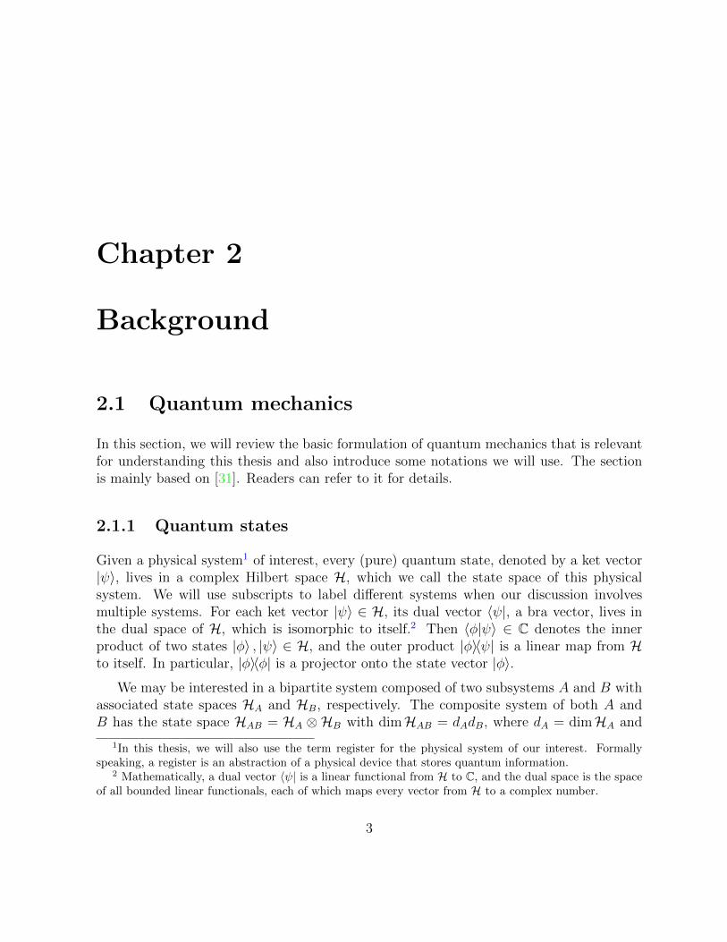
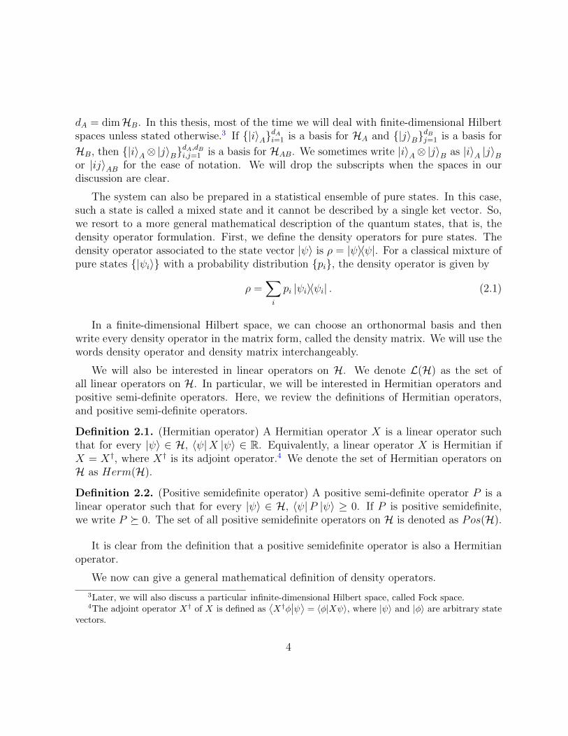

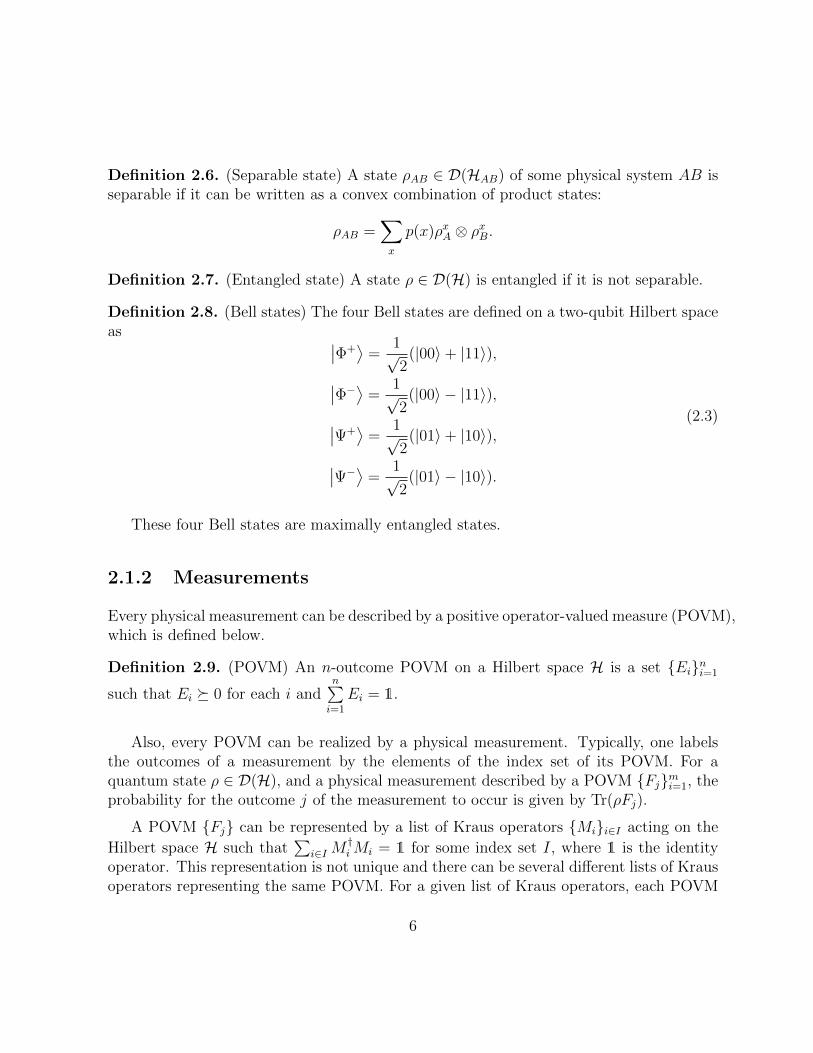


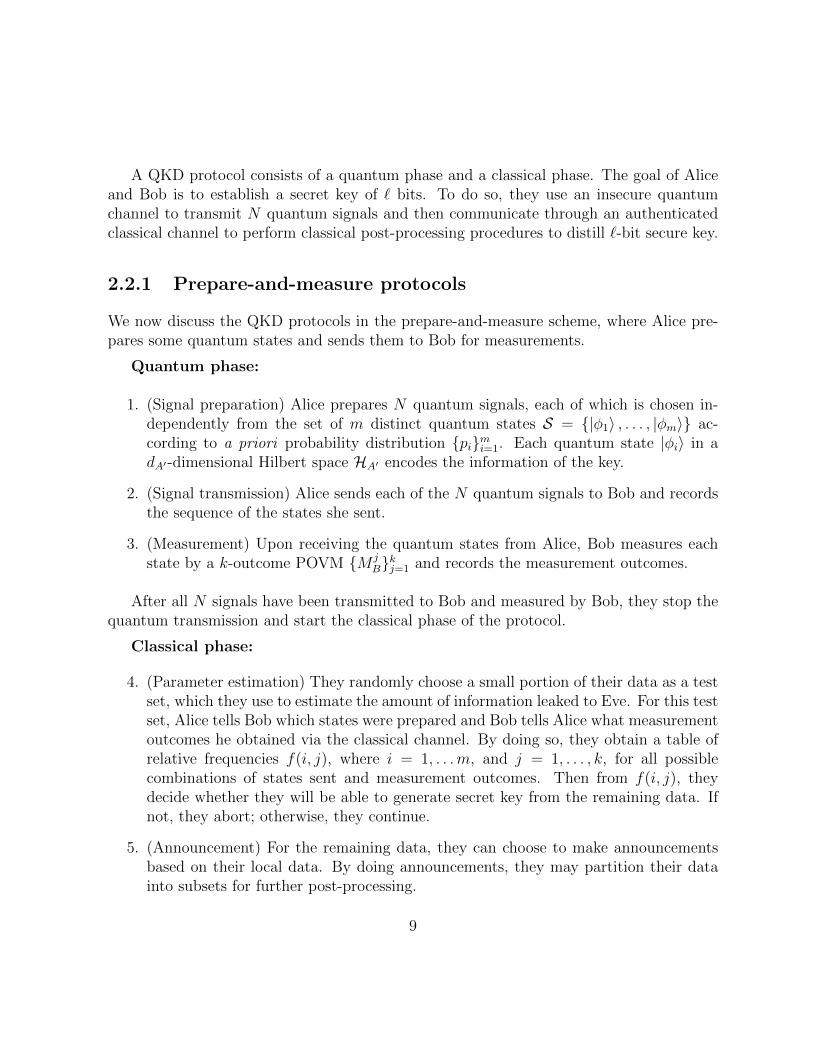


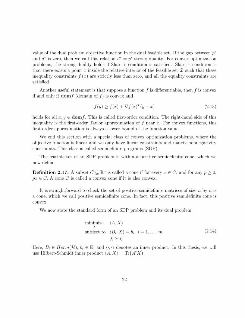
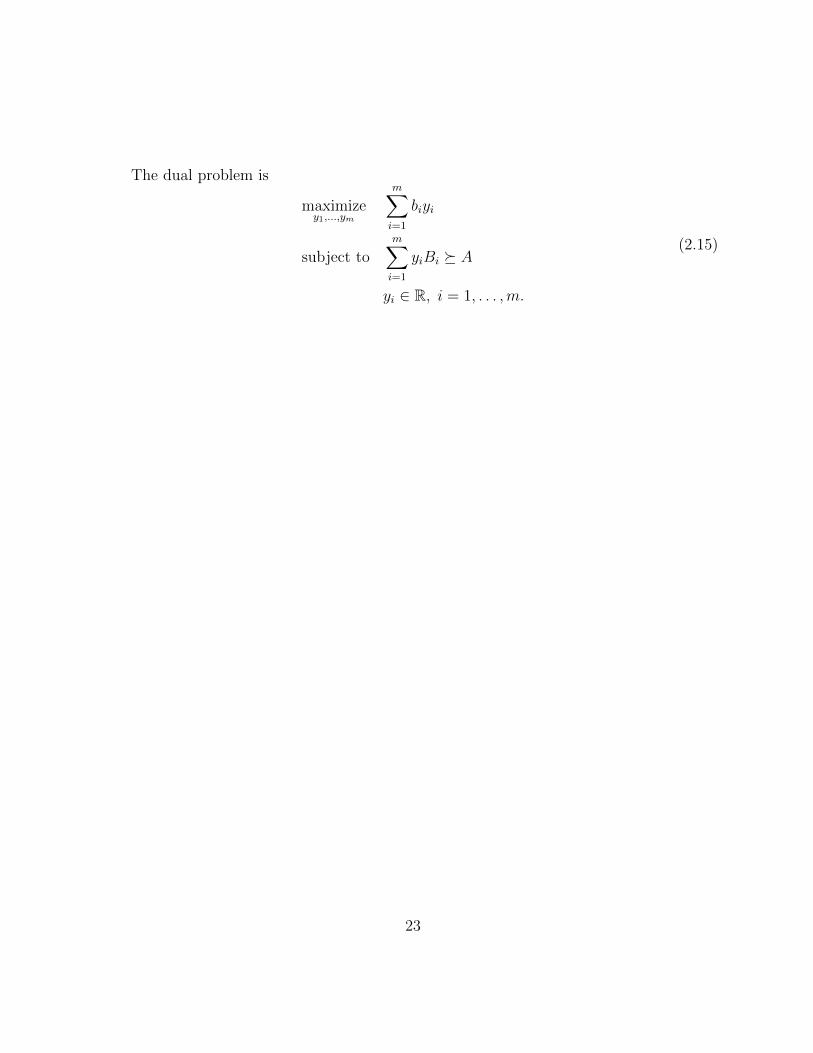


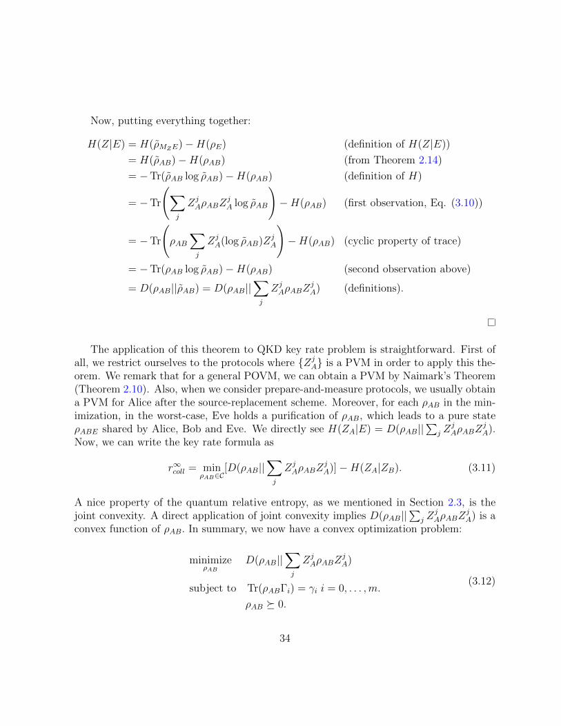
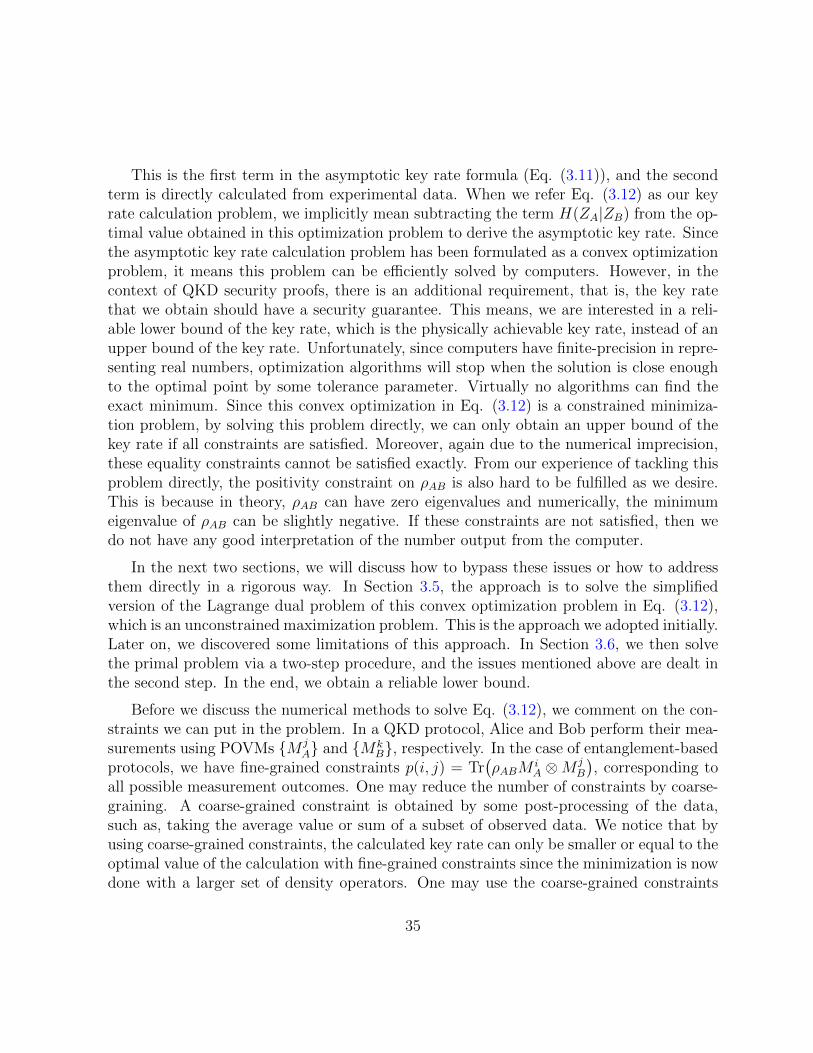


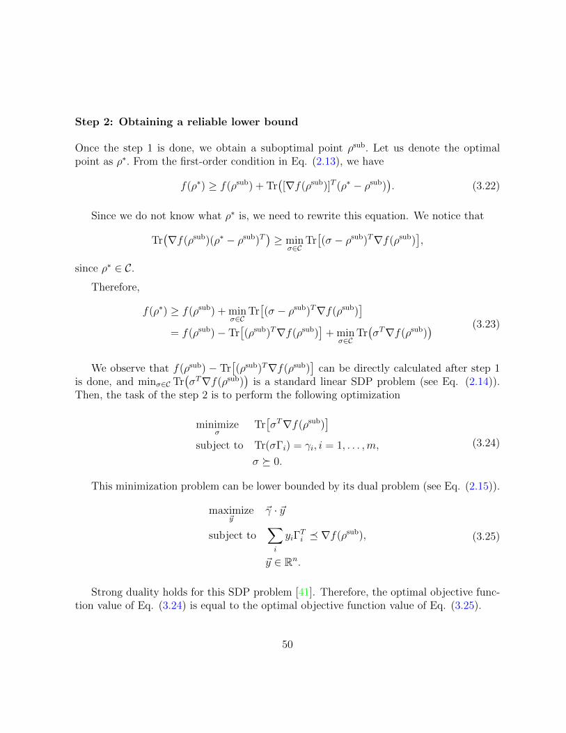


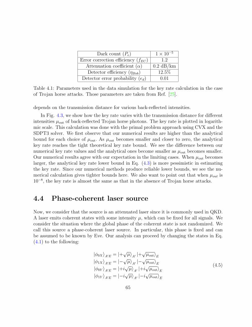


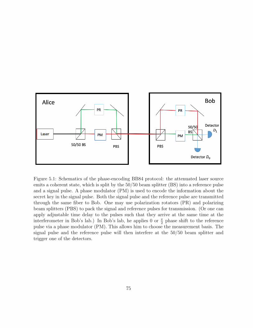
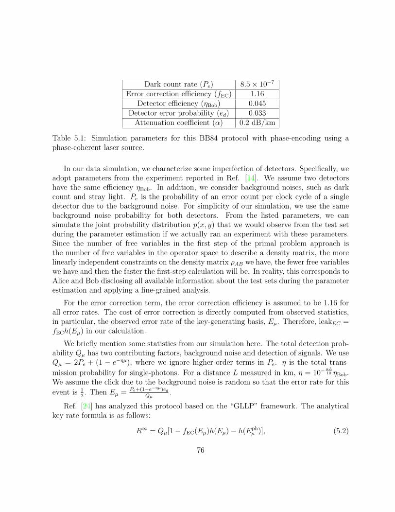

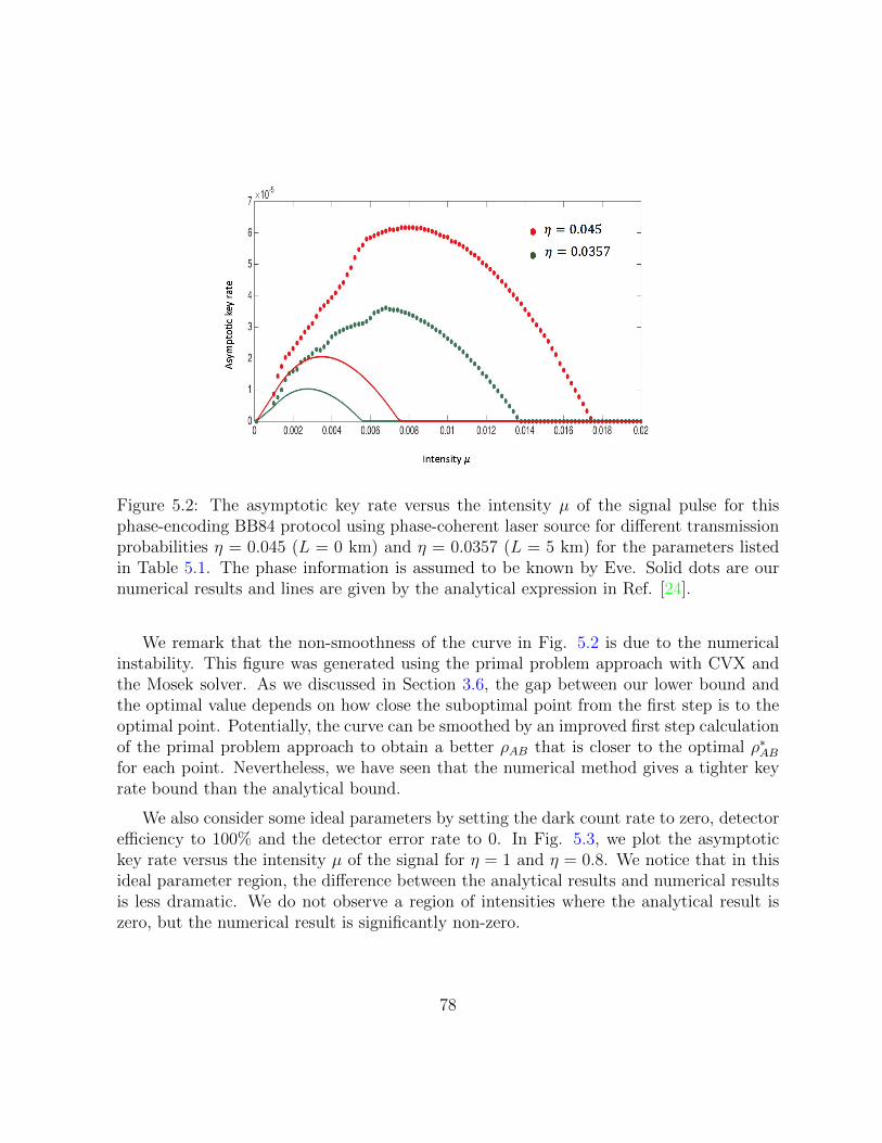


![Implementation Security of Quantum Cryptography...Quantum cryptography provides an ensemble of protocols, such as quantum key distribution [1-3], quantum random number generation [4],](https://static.documents.pub/doc/80x56/6132b6b7dfd10f4dd73aa066/implementation-security-of-quantum-cryptography-quantum-cryptography-provides.jpg)


