Page 1
Sede Amministrativa: Università degli Studi di Padova
Dipartimento di: Territorio e Sistemi Agro-Forestali (TESAF)
___________________________________________________________________
SCUOLA DI DOTTORATO DI RICERCA IN: TERRITORIO, AMBIENTE, RISORSE E SALUTE
CICLO: XXVII
TITOLO TESI: EVALUATION OF THE ENVIRONMENTAL IMPACTS OF WOOD PRODUCTS
FOR BIO-ENERGY THROUGH LIFE CYCLE ASSESSMENT (LCA)
Direttore della Scuola: Ch.mo Prof. Mario Aristide Lenzi
Supervisore: Prof. Tommaso Anfodillo
Dottorando : Francesca Pierobon
Page 5
Foreword
This research project was made possible thanks to the financial support of different institutions and
to the scientific contribution of many people to whom the author is most grateful.
For its entire length, the PhD was funded by the University of Padua through PhD research grant,
XXVII cycle. The research activities were primarily performed at the Department of Land,
Environment, Agriculture and Forestry of the University of Padua under the supervision of Prof.
Tommaso Anfodillo.
From February 17th, 2012 to December 31
st, 2012 the research was carried out in collaboration with
CSQA, Thiene (VI) and Fondazione E. Mach, S. Michele all’Adige (TN) and from January 9th,
2013 with IPLA, Turin.
From May 13th, 2013 to May 12
th, 2014 the research was carried out at at the School of
Environmental and Forest Sciences of the University of Washington, in Seattle, United States,
within the CINTRAFOR group under the supervision of Prof. Ivan Eastin. The work has been
developed as part of the NARA Project and partially funded by the University of Washington
through Grant no. 2011-68005-30416 from the USDA National Institute of Food and Agriculture.
Page 7
3
Abstract
The use of wood for energy has grown in the last years as an alternative to fossil fuels. National
and international laws promote the use of wood in the policies for the mitigation of climate change,
based on the assumption that wood has a neutral carbon balance because the combustion emissions
are offset by the absorption in forest (assumption of carbon neutrality). However, this assumption
does not take into account the emissions associated with the life cycle of the product, e.g. related to
processing and transporting biomass. In addition there is a time lag between the release of CO2
during combustion and its absorption in forest and this could have an impact on global warming.
The objectives of this research project are: 1) to assess the environmental impacts of wood products
through Life Cycle Assessment (LCA); 2) to include the dynamics of forest carbon sequestration
and natural decomposition of woody biomass in LCA. The research is conducted by means of two
case studies: the first is the LCA of firewood in the Northern East Italy; the second concerns the
production of wood chips in the Pacific Northwest in the United States. This dissertation consists in
eight chapters. Chapter 1 describes the legislative framework and the state of the art of the
international experiences and research projects on the subject. A review of literature studies was
conducted highlighting the main limitations and defining the research objectives. Chapters 2 and 3
analyze the supply chain of wood products for bioenergy, providing reference data for the biomass
extraction and production processes, the physico-chemical properties of wood and the LCA
methodology, in terms of standards, databases, softwares and methodologies. Chapters 4 and 5
present the results of the two case studies which identify the transportation to be the critical phase
of LCA, in the case of firewood related to the importation of raw materials from abroad, in the case
of chips related to the transportation on forest road. Chapter 6 deals with the assessment of carbon
sinks and stocks in the study areas previously analyzed. In Chapter 7 we face the problem of how
to include forest carbon sequestration within the LCA. This led to the development of a
methodology to perform a "dynamic LCA", which, in Chapter 8, is applied to a case study in the
Pacific Northwest. The methodology is based on the use of radiative forcing to evaluate the impact
of emissions and absorption sources on climate change. The results show that, in the case study
considered, a "Radiative Forcing Turning Point" exists, i.e. a point located approximately in the
middle of the forest rotation period (from 17 to 21 years old), where the life cycle impacts are
compensated by carbon dioxide absorption and beyond which the biomass produces a net benefit in
the carbon balance. The development of a dynamic LCA is very innovative in the context of LCA
and allowed to discuss the veracity of the assumption of carbon neutrality.
Page 9
5
Riassunto
L’uso di prodotti legnosi per fini energetici è cresciuto negli ultimi anni come alternativa ai
combustibili fossili. Leggi nazionali e internazionali promuovono l’uso del legno nell’ambito delle
politiche di mitigazione dei cambiamenti climatici, basandosi sull’assunzione che il legno abbia un
bilancio di carbonio nullo, in quanto le emissioni rilasciate dalla sua combustione vengono
compensate dagli assorbimenti in foresta (assunzione di carbon neutrality).Tuttavia, questa
assunzione non tiene in considerazione le emissioni associate al ciclo di vita del prodotto, e.g, alla
lavorazione e al trasporto della biomassa. Inoltre c’è uno sfasamento temporale tra il rilascio di
CO2 nella combustione e il suo assorbimento in foresta e questo potrebbe avere conseguenze sul
global warming. Gli obiettivi di questo progetto di ricerca sono: 1) valutare degli impatti ambientali
dei prodotti legnosi attraverso Life Cycle Assessment (LCA); 2) includere le dinamiche forestali di
assorbimento di anidride carbonica e decomposizione naturale della biomassa legnosa nell’LCA.
La ricerca è condotta per mezzo di due casi studio: il primo è costituito dall’LCA della legna da
ardere nel Nord-Est Italia; il secondo riguarda la produzione di cippato nell’area del Pacific
Northwest negli Stati Uniti. La tesi è costituita da otto capitoli. Nel Capitolo 1 si descrivono il
quadro legislativo e lo stato dell'arte delle esperienze internazionali e dei progetti di ricerca
sull’argomento. Viene inoltre effettuata una review di studi di letteratura mettendone in luce le
principali limitazioni e definendo gli obiettivi di ricerca. I Capitoli 2 e 3 analizzano la catena di
fornitura dei prodotti legnosi per fini energetici, fornendo dati di riferimento per i processi di
estrazione e produzione della biomassa e per le caratteristiche fisico-chimiche del legno e la
metodologia LCA, in termini di standard, banche dati, software e metodologie disponibili. I
Capitoli 4 e 5 presentano i risultati dei due casi studio che identificano nel trasporto la fase critica
dell’LCA, nel caso della legna da ardere legato all’importazione della materia prima dall’estero, nel
caso del cippato legato al trasporto su strada forestale. Il Capitolo 6 riguarda la valutazione dei
carbon sinks e stocks nelle aree di studio precedentemente analizzate. Nel capitolo 7 si affronta il
problema di come includere il sequestro di carbonio in foresta nell'ambito dell’LCA. Questo ha
portato allo sviluppo di una metodologia per effettuare un "LCA dinamico", che, nel Capitolo 8,
viene applicata ad un caso studio nel Pacific Northwest. La metodologia si base sull’utilizzo del
forzante radiativo per valutare l’impatto delle diverse fonti di emissioni ed assorbimento sul
cambiamento climatico. I risultati mostrano che, nel caso studio considerato, esiste un “Radiative
Forcing Turning Point”, ovvero un punto, situato circa a metà del periodo di rotazione della foresta
(tra 17 e 21 anni), dove gli impatti del ciclo di vita vengono compensati dagli assorbimenti di
anidride carbonica e oltre il quale la biomassa produce un beneficio netto in termini di bilancio del
carbonio. Lo sviluppo di un LCA dinamico è molto innovativo nel quadro dell’LCA e ha permesso
discutere la veridicità dell'assunto della carbon neutralità.
Page 11
7
Summary
The use of wood products for energy production has increased in the last years as an alternative to
fossil fuels. International and national regulations have supported the use of wood for energy since
it is considered to have a lower environmental impact than traditional energy sources (Cherubini et
al., 2009; Lippke et al., 2011b; Sathre and Gustavsson, 2012; Sathre and O’Connor, 2010). These
policies have been intensifying in the last period, setting more and more ambitious objectives for
the near future. As a consequence, it is expected that this sector will considerably increase in the
next years. For this reason, it is of fundamental importance to appropriately determine its
environmental impacts.
The approach initially adopted by the Kyoto Protocol for the evaluation of the sustainability of bio-
energy, which is still adopted in most of the environmental policies (EPA, 2011; IPCC, 2006;
United Nations, 1997) is based on the assumption of carbon neutrality, which affirms that the
carbon dioxide emissions generated during the biomass combustion equal the carbon dioxide
sequestered from the atmosphere by the trees for their growth attributing to the energy from
biomass an emission coefficient of zero (BSI, 2011; EPA, 2011; European Commission Joint
Research Centre, 2010).
However, other phases of the life cycle of wood products for bio-energy can play an important role
in the overall environmental impact. In fact, greenhouse gas emissions are released for the
consumption of fossil fuels and materials used in the forest operations of harvesting and processing
the wood in order to produce the biomass with the specific characteristics needed to be used to
produce energy. Furthermore, the transportation of the harvested wood can follow different paths,
depending on the morphology of the site and on the accessibility of the transportation means to the
harvesting site, thus releasing greenhouse gas emissions to the atmosphere, due to the fossil fuels
used in the transportation means. Moreover, if the raw materials are imported from abroad, long
distances have to be travelled in order to take the wood from the harvesting site to the processing
site. In addition, even though the use of wood has often been related to its benefit in terms of global
warming, some other aspects should be considered in evaluating the sustainability of bio-energy,
e.g. the combustion of wood can be critical for the local atmospheric pollution and the impact on
human health (Cespi et al., 2014; Solli et al., 2009).
For these reasons the evaluation approach initially adopted has been progressively replaced by
more global approaches which consider the whole emissions of the supply chain. The
internationally recognized approach is called Life Cycle Assessment (LCA) and, based on the ISO
14040-44, is defined as the “compilation and evaluation of the inputs, outputs and the potential
environmental impacts of a product system throughout its life cycle” (ISO, 2013a, 2006a). Through
the LCA it is possible to evaluate the impact on different impact categories, i.e. global warming,
Page 12
8
ozone depletion, eutrophication, acidification, smog formation, eco-toxicity, human health criteria,
human health cancer and human health non-cancer.
Even though the LCA is a powerful tool it is relatively recent and presents several limitations,
which have been outlined through the analysis of the scientific literature.
First of all it has been revealed that there is heterogeneity in the application of the methodology,
particularly regarding the system boundaries and the types of emissions included in the study. As
long as the Italian reality is concerned, a few studies about the impacts associated with the forest
operations have been found (Valente et al., 2011).
The carbon neutrality assumption is used in the majority of the LCA studies of biomass (Cherubini
et al., 2009; Helin et al., 2013; Lippke et al., 2011b; McKechnie et al., 2011; McManus, 2010;
Routa et al., 2012a, 2012b; Whittaker et al., 2011). This assumption is related to a specific
characteristic of the LCA, i.e. its static approach. In fact in LCA all the emissions and absorptions
are considered instantly released at the beginning of the evaluation period. Therefore the result is a
picture of the environmental impacts at a specific point in time. This represents a strong limitation
in the LCA studies, in fact the biomass growth in forest to regenerate the harvested wood can take a
long time depending on the forest management adopted and factors e.g. the rotation period, the type
of species, the age of the forest, the rate of harvesting. The rate of growth of biomass is related to
the rate of absorption of carbon dioxide from the atmosphere through the photosynthesis which has
a potential beneficial effect on global warming. Therefore, for wood products the carbon
sequestration may be crucial to determine the real impact on global warming of woody biomass
bio-energy. Also, the natural decomposition of wood in forest slowly releases greenhouse gases
over time and can take many decades to complete.
These aspects are not normally considered in LCA. In order to quantify them the traditional LCA
approach has to be extended and a dynamic approach should be used which considers the effect on
global warming of carbon dioxide emissions and removals according to a specific dynamic
function over time. To determine the real impact of bio-energy on global warming the impact in
terms of Radiative Forcing and its cumulative effect over time should be considered.
The following objectives have been defined:
1) Perform a Life Cycle Assessment of wood products for bio-energy to evaluate their
environmental impacts with the following specific targets (targets are subdivided for the specific
phases of the life cycle):
a. Raw materials supply:
Evaluation of the global and local impact of the transportation associated with the
importation of raw materials from abroad (long supply chain) compared to produce them
locally (short supply chain).
b. Production
Page 13
9
Evaluation of the environmental impact of the forest operations of harvesting and
processing the wood.
c. Distribution
Evaluation of the contribute of transportation in function of different logistics scenarios
based on the morphology of the site and the means of transportation adopted.
d. End of life:
Evaluation of the global and local impact of the wood combustion to produce bio-energy.
2) Incorporate dynamic functions of greenhouse gases release and uptake into the LCA framework
to develop a “dynamic LCA” for the following aspects:
a. Carbon sequestration in forest
Evaluation of the effect of forest management, considering the following factors: type of
species, disturbances, timeframe, type of management.
b. Decomposition of residues left in forest.
In Chapter 1 the legislative framework of bio-energy is described, including International,
European and National legislation and policies to mitigate climate change and the incentives
system for the energy produced from renewable sources. Furthermore the state of the art of the
international experiences and research projects about the evaluation of the environmental
performances of wood products for bio-energy are presented.
Chapter 2 describes the methodologies available for accounting the environmental impacts of bio-
energy, focusing on the Life Cycle Assessment approach, which is described based on international
standards. The chapter also analyzes the wood products supply chain for bio-energy. The state of
the art of the LCA studies of wood product for bioenergy has been reviewed and some limitation
outlined. This chapter also describes the motivation of the study, the research questions and the
objectives, which will be addressed through some case studies.
Chapter 3 analyzes the results of a Life Cycle Assessment of firewood. performed in North-Eastern
Italy. The focus of the study is to quantify the impact of the importation of the raw material from
abroad (Balkans area) on the impact categories Global Warming Potential (GWP), Ozone
Depletion Potential (ODP), Photochemical Ozone Creation Potential (POCP), Human Health
Potential (HTP) and to compare the long and the short supply chain. Also the local impact of the
wood combustion has been analyzed to determine its contribution on global and local scale to the
overall impact.
A sensitivity analysis has been performed to determine the critical distance of transportation for
impact categories. Lastly how to offset the carbon dioxide emissions of the overall life cycle has
been evaluated through forest management by saving a part of the biomass increment in forest.
Chapter 4 describes the results of a Life Cycle Assessment of wood chips performed in the U.S.
Pacific Northwest. The study focuses on the impact of different types of forest operations and
Page 14
10
logistics schemes by comparing a benchmark scenario with three alternate scenarios varying the
type of logistics, i.e. type of roads and distances travelled. The study also addressed the issues of
allocation and of the avoided impacts within the LCA. In this case, logs and residues are produced
from the forest and the impacts are allocated between the two products based on the mass flows.
Furthermore, in the Pacific Northwest, residues are generally piled and burned in forest. Their
recovery to produce bio-energy thus represents an avoided impact to the system.
A comparison of the results of the two case studies – firewood and wood chips - in terms of Global
Warming Potential has also been included in this chapter.
In Chapter 5 the problem of how to incorporate dynamic functions into the LCA framework has
been addressed. This has led to the development of a methodology to perform a “dynamic LCA” to
incorporate the dynamics of carbon sequestration and decomposition of wood into the LCA.
A new methodology has been studied and proposed which considers the Radiative Forcing of the
different sources of emissions and the decay of greenhouse gases to the atmosphere.
Through this approach it has been possible to discuss the truthfulness of the carbon neutrality
assumption.
The last section outlines the main findings of the research project. The environmental impacts of
wood products for bio-energy were evaluated in detail. Moreover a method has been proposed,
which has general validity and can be applied to every type of wood product.
The development of the dynamic LCA is very innovative in the LCA framework since neither in
LCA international standards nor in international politics this aspect has been introduced yet,
although it is beginning to spark the interest of the scientific community.
Given the sharp expected increase in the future in the use of biomass for the mitigation of climate
change, even small variations in the results could have enormous implications at global level.
The dynamic approach developed has contributed to fix some unsolved problems in the LCA
framework. In particular it can be applied to evaluate the impact of delayed emissions over time,
important aspect for both the evaluation of the carbon stored in long lasting wood products and the
delayed emissions for either natural decomposition or decomposition in landfill.
In conclusion it has been found that the biomass sustainability can vary according with many
factors. The type of forest management adopted in the harvesting site significantly influences the
impact on global warming as well as the residues quantity and the logistics. The application of this
approach could allow to define parameters in the international politics in favor of the types of
biomass which have the highest benefit on the global warming considering the impacts on the
overall supply chain.
Page 15
11
Acknowledgements
This research project is the result of the scientific contribution of many people to whom I am most
grateful. I would like to thank my adviser Prof. Tommaso Anfodillo, for having always supported
my work and for having led my research and made possible collaborations with national and
international institutions.
I would like to warmly thank Dott.ssa Michela Zanetti of the University of Padua, with whom the
time spent has been invaluable. For the whole length of my PhD Michela has been a reference
person to me and a source of inspiration and ideas.
I gratefully acknowledge Prof. Indoneil Ganguly and Prof. Eastin of the University of Washington
for the scientific contribution and the invaluable support.
I would kindly thank Prof. Raffaele Cavalli, Stefano Grigolato and Andrea Sgarbossa, Leonard
Bernardelli, Gian Battistel, Fabio Petrella , Lisa Causin and Silvia Stefanelli and all my friends of
the University of Padua and of the University of Washington.
I would like to express my most sincere gratitude to my family and a special thank to my friends
Federica and Stefano.
Page 17
13
Table of contents
Foreword ........................................................................................................................................... 1
Abstract ............................................................................................................................................. 3
Riassunto ........................................................................................................................................... 5
Summary ........................................................................................................................................... 7
Acknowledgements ......................................................................................................................... 11
Table of contents ............................................................................................................................ 13
List of figures .................................................................................................................................. 21
List of Tables .................................................................................................................................. 23
Chapter 1......................................................................................................................................... 27
Introduction and state of the art ................................................................................................... 27
1.1 Climate change ......................................................................................................................... 27
1.1.1 Observations data .............................................................................................................. 27
1.1.2 The cause of climate change ............................................................................................. 29
1.2 The International policy to mitigate climate change ............................................................. 30
1.2.1 The Kyoto Protocol ........................................................................................................... 30
1.2.2 Current ripartition of greenhouse gas emissions by country ............................................ 31
1.2.3 Towards a new international agreement post-Kyoto ........................................................ 34
1.3 Renewable energy to mitigate climate change ....................................................................... 35
1.3.1 Greenhouse gas emissions and the energy sector ............................................................. 35
1.3.2 The promotion of renewable energy and energy efficiency ............................................. 38
1.3.3 Incentives systems to the bio-energy production .............................................................. 41
1.3.3.1 The White Certificates or Energy Efficiency Certificates .................................... 41
1.3.3.2 The Green Certificates ......................................................................................... 42
1.3.3.3 All-inclusive fare .................................................................................................. 43
1.4 The use of wood for bio-energy ............................................................................................... 44
1.5 The environmental sustainability of woody biomass bio-energy ......................................... 45
Page 18
14
1.5.1 Life Cycle Assessment (LCA) .......................................................................................... 45
1.5.1.1 International LCA programs and standards .......................................................... 48
1.6 State of the art of LCA of wood products for bioenergy ...................................................... 50
1.6.1 Research projects about the evaluation of the environmental impacts of wood products 50
1.6.2 Literary review about LCA of woody biomass bio-energy .............................................. 51
1.6.2.1 Case studies and data availability ......................................................................... 53
1.6.2.2 Environmental benefits of replacing fossil fuels with bio-energy ........................ 54
1.6.2.3 Carbon neutrality .................................................................................................. 55
1.6.2.4 Harvesting, conversion and distribution phases ................................................... 57
1.6.2.5 Forest management .............................................................................................. 58
1.6.2.6 Dynamic LCA ...................................................................................................... 59
1.7 Motivation of the study ............................................................................................................ 61
1.8 Case studies ............................................................................................................................... 64
Chapter 2......................................................................................................................................... 65
The supply chain ............................................................................................................................ 65
2.1 The supply chain of wood products for bio-energy ............................................................... 65
2.1.1 Feedstock .......................................................................................................................... 65
2.1.2 Working phases and working systems .............................................................................. 65
2.1.3 Firewood production ......................................................................................................... 66
2.1.4 Wood chips production ..................................................................................................... 66
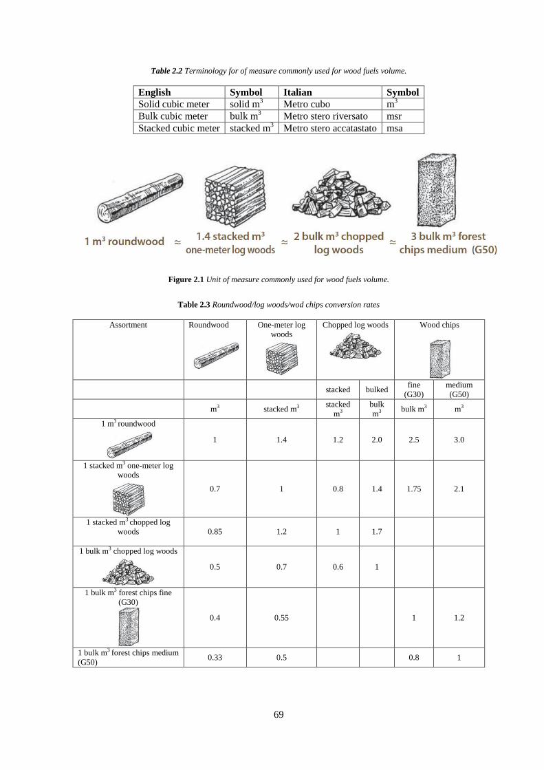
2.1.4.1 Volume terminology ............................................................................................ 68
2.1.5 Wood seasoning and drying .............................................................................................. 70
2.1.5.1 Water in wood ...................................................................................................... 70
2.1.5.2 Moisture content ................................................................................................... 71
2.1.5.3 Mass density of the main forest species ............................................................... 72
2.1.6 Technologies for energy production ................................................................................. 74
2.1.6.1 Firewood stoves.................................................................................................... 74
2.1.6.2 Wood chips stoves ................................................................................................ 74
Page 19
15
2.1.6.3 District heating networks ..................................................................................... 74
2.1.7 Factors influencing wood combustion .............................................................................. 74
2.1.7.1 Biomass chemical composition ............................................................................ 75
2.1.7.2 Ash content ........................................................................................................... 78
2.1.7.3 Calorific value and ashes ...................................................................................... 79
PART I ............................................................................................................................................ 81
Life Cycle Assessment of wood products for bioenergy ............................................................. 81
Chapter 3......................................................................................................................................... 83
Life Cycle Assessment of wood products – Materials and methods .......................................... 83
3.1 Life Cycle Assessment methodology ....................................................................................... 83
3.1.1 Goal and scope definition ................................................................................................. 84
3.1.2 1.2 Life cycle inventory analysis (LCI) ............................................................................ 85
3.1.3 Life cycle impact assessment (LCIA) ............................................................................... 86
3.1.4 1.4 Life cycle interpretation .............................................................................................. 87
3.2 2. LCA computational model .................................................................................................. 87
3.2.1 2.1 Simplified model for inventory analysis ..................................................................... 87
3.2.1.1 Unit process .......................................................................................................... 87
3.2.1.2 System .................................................................................................................. 88
3.2.1.3 Partitioned matrix ................................................................................................. 88
3.2.1.4 Specification of the required performance of the system. .................................... 88
3.2.2 2.2 General model for inventory analysis ......................................................................... 89
3.2.2.1 Cut off economic flows ........................................................................................ 89
3.2.2.2 Process alternatives .............................................................................................. 89
3.2.2.3 Multifunctional processes .................................................................................... 89
3.2.2.4 Closed loop recycling ........................................................................................... 90
3.3 3. LCA databases ...................................................................................................................... 91
3.4 4.LCA Softwaress ..................................................................................................................... 94
3.4.1 4.1 Greenhouse Gases, Regulated Emissions and Energy Use in Transportation (GREET)
Model ......................................................................................................................................... 94
Page 20
16
3.4.2 4.2 SimaPro software ........................................................................................................ 95
3.4.3 4.3 Gabi software .............................................................................................................. 95
3.5 5. Impact assessment methods ................................................................................................. 96
3.5.1 CML-IA ............................................................................................................................ 96
3.5.2 Ecological scarcity 2013 ................................................................................................... 97
3.5.3 EDIP 2003 ........................................................................................................................ 97
3.5.4 EPD (2013) ....................................................................................................................... 97
3.5.5 EPS 2000 .......................................................................................................................... 97
3.5.6 Impact 2002+ .................................................................................................................... 98
3.5.7 ReCiPe .............................................................................................................................. 99
3.5.8 ILCD 2011 Midpoint+ ...................................................................................................... 99
3.5.9 BEES............................................................................................................................... 100
3.5.10 TRACI 2.1 .................................................................................................................... 100
3.6 6. Impact categories overview ............................................................................................... 100
3.6.1 Climate change ............................................................................................................... 102
3.6.2 Stratospheric Ozone depletion ........................................................................................ 102
3.6.3 Human toxicity ............................................................................................................... 102
3.6.4 Acidification ................................................................................................................... 103
3.6.5 Eutrophication ................................................................................................................. 103
3.6.6 Eco-toxicity ..................................................................................................................... 103
3.6.7 Photochemical Ozone Creation Potential (POCP) .......................................................... 104
3.6.8 Land use .......................................................................................................................... 104
3.6.9 Depletion of abiotic resources ........................................................................................ 104
3.6.10 Habitat and ecosystems ................................................................................................. 105
3.6.11 Ionizing radiation .......................................................................................................... 105
Chapter 4....................................................................................................................................... 107
Life Cycle Assessment of firewood for domestic heating .......................................................... 107
4.1 Abstract ................................................................................................................................... 107
Page 21
17
4.2 Introduction ............................................................................................................................ 107
4.3 Materials and methods........................................................................................................... 109
4.4 Results ..................................................................................................................................... 113
1. Environmental impacts of the short and long supply chain. .......................................... 113
2. Sensitivity analysis for the evaluation of the critical distance of transportation ............ 117
3. Carbon offsetting in forest .............................................................................................. 119
4.5 Discussion ................................................................................................................................ 120
4.6 Conclusions ............................................................................................................................. 122
Chapter 5....................................................................................................................................... 125
Life Cycle Assessment of wood chips for bio-energy ................................................................ 125
5.1 The NARA Project ................................................................................................................. 125
5.2 The CORRIM Database ........................................................................................................ 127
5.3 Abstract ................................................................................................................................... 131
5.4 Introduction ............................................................................................................................ 131
5.5 Materials and methods........................................................................................................... 133
5.5.1 System boundary ............................................................................................................ 133
5.5.2 Woody Biomass Collection and Processing ................................................................... 134
5.5.3 Feedstock Logistics ........................................................................................................ 137
5.5.4 Biomass combustion and heat production ...................................................................... 140
5.5.5 Avoided impacts of slash piles burning .......................................................................... 141
5.5.6 Comparative Analysis: Global Warming Potential of wood chips vs firewood ............. 144
5.6 Analysis and results ................................................................................................................ 146
5.6.1 Results of the LCA of wood chips .................................................................................. 146
5.6.2 Avoided Environmental Burdens of Slash Pile Burning ................................................ 147
5.6.3 Comparison of the results of the two case studies in terms of Global Warming Potential
................................................................................................................................................. 149
5.7 Conclusions ............................................................................................................................. 151
PART II ......................................................................................................................................... 153
Dynamic Life Cycle Assessment .................................................................................................. 153
Page 22
18
Chapter 6....................................................................................................................................... 155
Carbon sinks and stocks evaluation ........................................................................................... 155
6.1 Introduction ............................................................................................................................ 155
6.2 Materials and methods........................................................................................................... 155
6.3 Areas of the study ................................................................................................................... 158
6.3.1 Italian Alps. ..................................................................................................................... 158
6.3.2 US Pacific Northwest. .................................................................................................... 159
6.4 Case studies: ........................................................................................................................... 159
6.4.1 .1Italian Alps ................................................................................................................... 159
6.4.1.1 Veneto Region .................................................................................................... 160
6.4.1.2 Autonomous Province of Trento ........................................................................ 161
6.4.1.3 Piemonte Region ................................................................................................ 162
6.5 Results ..................................................................................................................................... 162
Chapter 7....................................................................................................................................... 167
Numerical approach to include time dependent natural phenomena dynamics, delayed
emissions and carbon storage into the LCA .............................................................................. 167
7.1 Introduction ............................................................................................................................ 167
7.2 Methodological review ........................................................................................................... 168
7.2.1 The Radiative Forcing concept ....................................................................................... 168
7.2.2 Natural phenomena dynamics ......................................................................................... 172
7.2.3 Carbon storage and delayed emissions ........................................................................... 172
7.2.3.1 The Moura-Costa method ................................................................................... 173
7.2.3.2 The Lashof accounting ....................................................................................... 174
7.2.3.3 The PAS 2050 .................................................................................................... 175
7.3 Methodology developed to include temporal aspects into the LCA ................................... 176
7.3.1 Materials and methods .................................................................................................... 177
7.4 Conclusions ............................................................................................................................. 181
Chapter 8....................................................................................................................................... 183
Page 23
19
Development of a Dynamic Life Cycle Assessment through the Radiative Forcing
methodology .................................................................................................................................. 183
8.1 Abstract ................................................................................................................................... 183
8.2 Introduction ............................................................................................................................ 183
8.3 Materials and Methods .......................................................................................................... 185
8.3.1 Area of study ................................................................................................................... 185
8.3.2 System boundary ............................................................................................................ 185
8.3.3 Carbon sequestration ...................................................................................................... 186
8.3.4 Harvest operations .......................................................................................................... 188
8.3.5 Residues left in the forest................................................................................................ 190
8.3.6 Burning biomass ............................................................................................................. 191
8.3.7 Evaluation of the impact on global warming through radiative forcing ......................... 192
8.4 Results ..................................................................................................................................... 194
8.5 Discussion ................................................................................................................................ 197
8.6 Conclusions ............................................................................................................................. 198
8.7 Acknowledgements ................................................................................................................. 199
Conclusions ................................................................................................................................... 201
8.1 Innovative aspects of this study ............................................................................................. 203
References ..................................................................................................................................... 205
Page 25
21
List of figures
Figure 1.1 Observed global mean combined land and ocean surface temperature anomalies, from
1850 to 2012 ( IPCC 2013). ............................................................................................................. 27
Figure 1.2 Multiple observed indicators of a changing global climate: (a) Extent of Northern
Hemisphere spring average snow cover; (b) extent of summer average sea ice; (c) change in global
mean upper ocean (0–700 m) heat content aligned to 2006−2010, and relative to the mean of all
datasets for 1970; (d) global mean sea level relative to 1900. (IPCC, 2013). ................................. 28
Figure 1.3 Representation of the world ripartition between Annex I and non-Annex I Parties ...... 31
Figure 1.4 Top 10 emitting countries in 2011 (IEA, 2013). ............................................................ 32
Figure 1.5 CO2 emissions annual growth rate by region (2010-11) (IEA, 2013). .......................... 32
Figure 1.6 CO2 emissions per capita by major world regions ( IEA, 2013). ................................... 33
Figure 1.7 CO2 emissions per GDP by major world regions ( IEA, 2013). .................................... 33
Figure 1.8 World CO2 emissions by sector in 2011 (IEA, 2013). ................................................... 35
Figure 1.9 Shares of anthropogenic GHG emissions in Annex I countries, 2011 ( IEA, 2013). .... 36
Figure 1.10 World primary energy supply and CO2 emissions: shares by fuel in 2011 (IEA, 2013).
.......................................................................................................................................................... 36
Figure 1.11 CO2 emissions from electricity and heat generation (IEA, 2013). ............................... 37
Figure 1.12 World primary energy supply (IEA, 2013). ................................................................. 38
Figure 1.13 Representation of the carbon cycle. ............................................................................. 45
Figure 1.14 Ripartition of the topic addressed in the review papers. .............................................. 52
Figure 1.15 Ripartition of the first author’s organization countries of the review papers............... 52
Figure 1.16 Ripartition of the years of publication of the review papers. ...................................... 53
Figure 2.1 Firewood and wood chips for bioenergy. ....................................................................... 65
Figure 2.3 Unit of measure commonly used for wood fuels volume. ............................................. 69
Figure 2.5 Representation of micro and macroporosity in wood. ................................................... 71
Figure 2.9 Woody biomass components: cellulose, hemicelluloses and lignin. ............................. 75
Figure 3.1 Phases of the LCA (ISO 14040). ................................................................................... 83
Figure 3.3 Screenshot of the SimaPro v.8 interface. ...................................................................... 95
Figure 3.4 Screenshot of Gabi v.5 interface. ................................................................................... 96
Figure 3.5 Scheme of the Impact 2002+ LCA evaluation method (PRé Consultants, 2014). ......... 98
Figure 4.1 Process flow diagram of the investigated firewood supply-chain................................ 110
Figure 4.4 Short and long firewood supply chains comparison in term of environmental impacts
(GWP=Global Warming Potential; ODP=Ozone Depletion Potential; POCP=Photochemical Ozone
Creation Potential; HTP=Human Toxicity Potential. Note: the biogenic CO2 has not taken into
account in the GWP) ...................................................................................................................... 114
Page 26
22
Figure 4.6 Sensitivity analysis for (a) g CO2 – eq and (b) g R11 – eq emissions as a function of the
road transport phase distance. ........................................................................................................ 118
Figure 4.7 Sensitivity analysis for (a) mg Ethene – eq and (b) g DCB – eq emissions as a function
of the road transport phase distance. .............................................................................................. 119
Figure 5.1 Organizations participating in the NARA Project. ...................................................... 126
Figure 5.3 System boundaries of the Life Cycle Assessment of wood chips. ............................... 133
Figure 5.4 Regional Scope of Study (courtesy Natalie Martinkus) ............................................... 134
Figure 5.13 Piling and burning woody residuals in forest is a common practice in the U.S. Pacific
Northwest. ...................................................................................................................................... 141
Figure 5.19 Comparison of the system boundaries. ...................................................................... 145
Figure 5.20 Processes contribution to global warming, ozone depletion and photochemical smog
potentials.The results are referred to 1 MJ of energy. .................................................................... 146
Figure 5.23 Global warming potential of alternate feedstock scenarios for 1 MJ of energy. ...... 148
Figure 5.25 LCA results comparison excluding the avoided impacts from slash piles (left) and
including them (right). ................................................................................................................... 150
Figure 5.26 Comparison of the process contribution of the LCA of wood chips (benchmark
scenario) and the LCA of firewood (short supply chain). .............................................................. 150
Figure 5.27 Comparison of the process contribution of the LCA of wood chips (benchmark
scenario) and the LCA of firewood (short supply chain). .............................................................. 151
Figure 6.1 Area of study of Italian Alps. ....................................................................................... 158
Figure 7.3 Decay of 1 kg pulse of GHGs. ..................................................................................... 170
Figure 7.5 Rappresentation of the Moura-Costa method. ............................................................. 173
Figure 7.6 Rappresentation of the Lashof accounting method. ..................................................... 174
Figure 8.1 System boundaries of the LCA ................................................................................... 186
Figure 8.2. Representation of the carbon balance in forest. .......................................................... 186
Figure 8.3 Decay function of GHGs. ............................................................................................ 193
Figure 8.4 Difference of biomass growth between subsequent years (carbon sink) and carbon
biomass (carbon stock) over time normalized to the functional unit (1 BDmT) expressed in terms
of carbon dioxide absorbed. ........................................................................................................... 194
Figure 8.5 Decomposition of residues left in forest. ..................................................................... 196
Figure 8.6 .Result of the evaluation of the impact on global warming through the Radiative
Forcing. .......................................................................................................................................... 196
Page 27
23
List of Tables
Table 2.1 Technical characteristics of common working machines used in forest operations
(AEBIOM, 2009). ............................................................................................................................ 67
Table 2.2 Terminology for of measure commonly used for wood fuels volume. ........................... 69
Table 2.3 Roundwood/log woods/wod chips conversion rates........................................................ 69
Table 2.4 Softwood, mean values of mass density with moisture content (MC) 13% (Giordano,
1988). ............................................................................................................................................... 72
Table 2.5 Hardwood, mean values of mass density with moisture content (MC) 13% (Giordano,
1988). ............................................................................................................................................... 73
Table 2.6 Bulk density in kg of the main solid biofuels (AEBIOM, 2009) (the equivalence 1m3
roundwood = 2.43 bulk m3 (volumetric index=0.41 m
3/bulk m
3) of wood chips has been used) .... 73
Table 2.7 Structural composition of wood (wt.% of dry and ash-free sample) ............................... 76
Table 2.8 Chemical composition of solid biomass (AEBIOM, 2009). ............................................ 77
Table 2.9 Ash content in bark, wood chips,saw dust and straw (AEBIOM, 2009). ........................ 78
Table 2.10 Calorific valuesof wood in function of the moisture content (AEBIOM, 2009). ......... 80
Table 3.1 Description of the main LCA database............................................................................ 92
Table 3.2 Comparison of the impact categories included in LCA methods. ................................. 101
Table 4.1 Relative contributions of the short supply chain processes to global warming potential
(GWP), ozone depletion potential (ODP), photochemical ozone creation potential (POCP) and
human toxicity potential (HTP) for the production of 1MJ of energy. Note: the biogenic CO2 has
not taken into account in the GWP ................................................................................................. 113
Table 4.2 Relative contributions of the long supply chain processes to global warming potential
(GWP), ozone depletion potential (ODP), photochemical ozone creation potential (POCP) and
human toxicity potential (HTP) for the production of 1MJ of energy. Note: the biogenic CO2 has
not taken into account in the GWP ................................................................................................. 113
Table 4.3 Relative contributions of chemicals in the short and in the long supply chain for the
production of 1MJ of energy. The values are referred to the emissions after characterization
(“Characterization” column) and before characterization (“Inventory” column) for global warming
potential (GWP), ozone depletion potential (ODP), photochemical ozone creation potential (POCP)
and human toxicity potential (HTP) ............................................................................................... 115
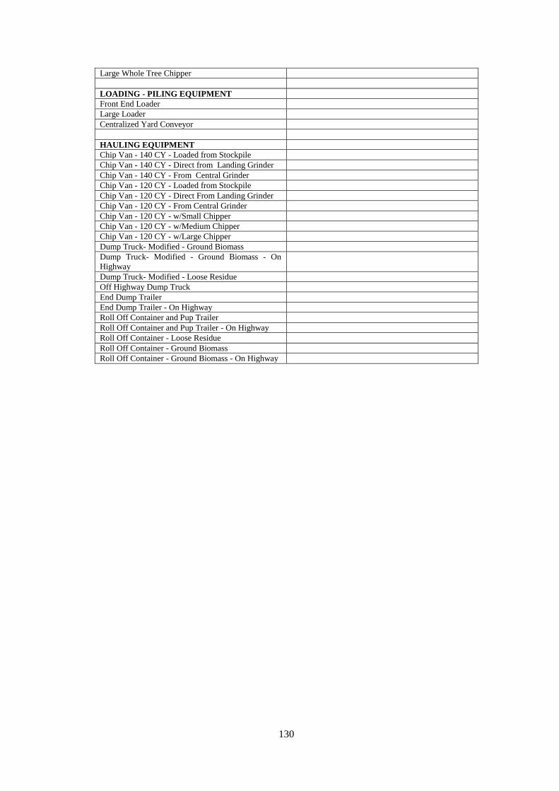
Table 5.1 List of forest equipments included in the CORRIM database. ...................................... 129
Table 5.2 Diesel and lubricants consumption of forest equipments ( CORRIM database). .......... 136
Table 5.3 Inputs and outputs of the harvesting process. ................................................................ 136
Table 5.4 Equipment configuration of the benchmark scenario. ................................................... 137
Table 5.5Benchmark scenario for road-type specific transportation distances. ............................ 137
Page 28
24
Table 5.6 Equipment configuration of the alternate scenarios. ..................................................... 138
Table 5.7 Alternate scenarios for road-type specific transportation distances. ............................. 138
Table 5.8 Energy and material consumption for 1 BDmT of wood chips, 30 CY dump truck. .... 140
Table 5.9 Energy and material consumption for 1 BDmT of wood chips, 50 CY roll off. ........... 140
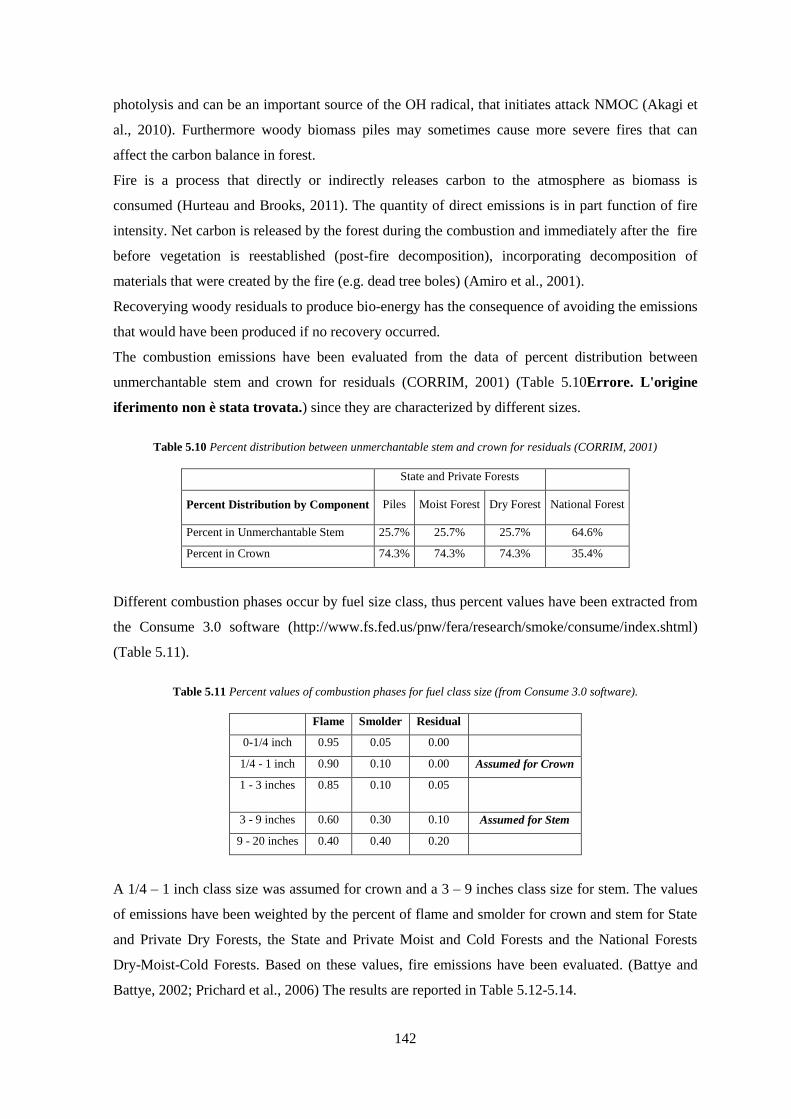
Table 5.10 Percent distribution between unmerchantable stem and crown for residuals (CORRIM,
2001) .............................................................................................................................................. 142
Table 5.11 Percent values of combustion phases for fuel class size (from Consume 3.0 software).
........................................................................................................................................................ 142
Table 5.12 Fires emissions estimation for State and Private Dry Forests. .................................... 143
Table 5.13 Fires emissions estimation for State and Private Moist and Cold Forests. .................. 143
Table 5.14 Fires emissions estimation for National Dry-Moist-Cold Forests. .............................. 144
Table 5.15 Alternate scenario for road-type specific transportation distances. ............................. 147
Table 5.16 LCA results for the six scenarios, referred to 1 MJ of energy. ................................... 147
Table 5.17 Net LCA results for the benchmark scenario including avoided impacst. .................. 149
Table 6.1 Summary of some data collected for the Vicenza Province in Veneto Region. ............ 160
Table 6.2 Summary of some data collected for the Belluno Province in Veneto Region. ............ 160
Table 6.3 Summary of some data collected for the Autonomous Province of Trento................... 161
Table 6.4 Summary of some data collected for the Val Varaita in Piemonte Region. .................. 162
Table 6.5 Results of forest carbon sequestration evaluation for some municipalities in Vicenza
Province in Veneto Region. ........................................................................................................... 162
Table 6.6 Results of forest carbon sequestration evaluation for some municipalities in Belluno
Province in Veneto Region. ........................................................................................................... 163
Table 6.7 Results of forest carbon sequestration evaluation for some municipalities in Autonomous
Province of Trento. ......................................................................................................................... 163
Table 6.8 Results of forest carbon sequestration evaluation in Val Varaita in Piemonte Region. 163
Table 6.9 Summary of some data collected for the Western Montana Corridor, US. ................... 165
Table 6.10 Results of forest carbon sequestration evaluation in Western Montana Corridor, US. 165
Table 6.11 Comparison of results of forest carbon sequestration evaluation between Italian Alps
and Western Montana Corridor, US. .............................................................................................. 166
Table 7.1GHGs lifetimes according to the 4th and 5
th IPCC Report. ............................................. 169
Table 7.2 Parameters values for the decay function of a pulse of CO2 according to the 4th and 5
th
IPCC Report. .................................................................................................................................. 169
Table 7.3 Background concentrations (C0), radiative efficiency (RE) and radiative forcing (RF ) of
CO2, CH4 and N2O reported in the 4thand in the 5
th IPCC Report. ................................................. 171
Table 8.1 Hourly consumption of diesel and lubricants of machines and transport means used in
forest operations. ............................................................................................................................ 189
Page 29
25
Table 8.2 Time of usage of machines and transport means used for forest operations per ton of
woody biomass harvested............................................................................................................... 189
Table 8.3 Emissions to air from the burning of 1 BDmT of biomass........................................... 192
Table 8.4 Greenhouse gas emission from forest operations. ........................................................ 195
Page 31
27
Chapter 1
Introduction and state of the art
1.1 Climate change
1.1.1 Observations data
Climate change represents one of the major threats of this century. The global average temperature
has been dramatically increasing in the last years causing average atmosphere and ocean warming.
According to the 5th IPCC Report, global warming is unequivocal and since 1950s, many of the
observed changes are unprecedented over decades to millennia. The globally averaged combined
land and ocean surface temperature data show a warming of 0.85 [0.65 to 1.06] °C, over the period
1880 to 2012. The total increase between the average of the 1850–1900 period and the 2003–2012
period is 0.78 [0.72 to 0.85] °C, based on the single longest dataset available (IPCC, 2013).
Figure 1.1 Observed global mean combined land and ocean surface temperature anomalies, from 1850 to 2012 ( IPCC
2013).
Page 32
28
The global temperature increase is altering the equilibrium of natural ecosystem, including the
water and the energy balances and the carbon cycle. The temperature increase is causing an
extensive melting of glaciers and snowfields, an increase of the oceans temperature, and a global
rise of sea level.
Figure 1.2 Multiple observed indicators of a changing global climate: (a) Extent of Northern Hemisphere spring average
snow cover; (b) extent of summer average sea ice; (c) change in global mean upper ocean (0–700 m) heat content
aligned to 2006−2010, and relative to the mean of all datasets for 1970; (d) global mean sea level relative to 1900.
(IPCC, 2013).
Page 33
29
The IPCC updated data show that, over the period 1993 to 2009, the average rate of ice loss from
glaciers around the world was 275 Gt yr−1
, significantly higher than the value registered over the
period 1971 to 2009, which was 226 Gt yr−1
. The average rate of ice loss over the period 2002 to
2011 was more than six times higher than the one registered over the period 1992 to 2001 from the
Greenland ice sheet and almost five times higher from the Antarctic ice sheet. The Antarctic sea ice
extent increased at a rate in the range of 1.2 to 1.8% per decade.
Climate change has also been causing dramatic increase of the sea level. According to the IPCC,
the rate of sea level rise since the mid-19th century has been larger than the mean rate during the
previous two millennia. The mean rate of global averaged sea level rise was 1.7 mm yr-1
between
1901 and 2010, 3.2 mm yr-1
between 1993 and 2010.
Changes in the global water cycle in response to the warming also includes increase in contrast in
precipitation between wet and dry regions and between wet and dry seasons.
1.1.2 The cause of climate change
Global warming is associated with the presence in the atmosphere of certain gases, called
greenhouse gases (GHG) in higher concentrations than those naturally present. GHGs, natural or
anthropogenic, absorb and emit radiation at specific wavelengths within the spectrum of infrared
radiation emitted by the Earth's surface, atmosphere and clouds.
The main GHGs are:
- Carbon dioxide (CO2)
- Methane (CH4)
- Nitrous oxide (N2O)
- Halocarbons (chlorofluorocarbons (CFCs), hydrochlorofluorocarbons (HCFCs),
hydrofluorocarbons (HFCs), perfluorocarbons)
- Sulfur hexafluoride (SF6).
It is unequivocal that anthropogenic increases in the well-mixed greenhouse gases have
substantially enhanced the greenhouse effect (IPCC, 2013). The atmospheric concentrations of
greenhouse gases have increased to levels unprecedented in at least the last 800 000 years at
increasing growing rate, due to human activity, since the industrial revolution.
In 2011 the concentrations of carbon dioxide, methane and nitrous oxide were 391 ppm, 1803 ppb,
and 324 ppb, and exceeded the pre-industrial levels by about 40%, 150%, and 20%, respectively
(IPCC, 2013).
Global Warming is measured through the Radiative Forcing (RF), which is a measure of the change
in energy fluxes caused by changes in these drivers. The total anthropogenic RF for 2011 relative
to 1750 was 2.29 [1.13 to 3.33] W m−2
, and it has increased more rapidly since 1970 than during
prior decades. The total anthropogenic RF best estimate for 2011 is 43% higher than that reported
Page 34
30
in AR4 for the year 2005 (IPCC, 2013).
Climate change will have inevitable economic consequences for the countries that will have to bear
the costs for the actions of adaptation and mitigation and social because it will lead to a shrinking
resource and worsening living conditions.
According to the latest IPCC Report, global warming is unequivocal, however, reducing the
emissions of greenhouse gases in sufficient concentration to stabilize the increase in average global
temperature to 2 ° C can significantly limit the damage on ecological systems, social and economic
globally.
For this reason, the reduction of greenhouse gas emissions is considered an environmental priority
and is the main focus of political and institutional debates. Many actions have been undertaken at
different levels to mitigate climate change by imposing obligations to reduce emissions globally.
1.2 The International policy to mitigate climate change
1.2.1 The Kyoto Protocol
The environmental problem began to be discussed at international level in the ‘80s. In 1980 the
World Meteorological Organization (WMO) organized the First International Conference for the
climate, during which concern was expressed about the energetic balance of the earth and its
possible consequences on the atmosphere and on the climate. In 1987 the concept of sustainable
development was first defined in the Bruntland Report as the “development that meets the needs of
the present without compromising the ability of future generations to meet their own needs”
(United Nations, 1987).
In order to collect and disseminate information about global warming and its risks in 1988 the
World Meteorological Organization (WMO) and the United Nations Environmental Program
(UNEP) instituted the Intergovernmental Panel on Climate Change (IPCC). Every five years the
IPCC produces a Report with updated data about the physical basis of climate change, the
mitigation strategies and the adaptation actions to adopt.
A fundamental step in the international legislation about climate change was signed by the United
Nations Conference on Environment and Development in Rio de Janeiro in 1992 (United Nations,
1992a) during which the United Nations Framework Convention on Climate Change (UNFCCC)
was instituted, an international environmental agreement entered into force in 1994 (United
Nations, 1992b). Since then the Convention parties have been meeting once every year in a
"Conference of Parties" (COP) to discuss about the climate change and mitigation strategies.
During the COP3, in 1997 in Kyoto, the first international agreement about climate change, the
Kyoto Protocol, was signed, (United Nations, 1997). The Kyoto Protocol is an executive act which
contains reduction objectives and targets to reduce the greenhouse gas emissions by 5.2%
Page 35
31
compared to the 1990 values by the commitment period 2008-2012 based on the historical
emissions levels of each country. The UNFCCC divides countries in two groups:
- “Annex I” parties: industrialized countries considered historically responsible of the GHG
emissions, thus subject to reduction objectives, as opposed to “Non-Annex I” parties,
constituted by developing countries not subject to reduction objectives.
- “Annex II” parties: industrialized countries required to financially support mitigation ad
adaptation to climate change in developing countries.
Thus specific reduction objectives were set for the Annex I parties as follow: European Union: -
8%, United States -7%, Japan -6%, Russia, Ukraine, New Zealand 0%, Norway +1%, Australia
+8%, Island +10%. The Kyoto Protocol entered into force in 2005, after the ratification of Russia
and ended in 2012 at the end of the commitment period 2008-2012.
Annex I Parties Non-Annex I Parties
Figure 1.3 Representation of the world ripartition between Annex I and non-Annex I Parties
Close to the end of the Kyoto Protocol commitment period, the international committee started to
discuss the need of negotiating a new global agreement for the period after Kyoto. As described in
the next paragraph, the international political and economical situation is now completely changed
compared to the time when the Kyoto Protocol was signed, since developing country emissions
surpassed those of industrialized countries, and have kept rising very rapidly.
1.2.2 Current ripartition of greenhouse gas emissions by country
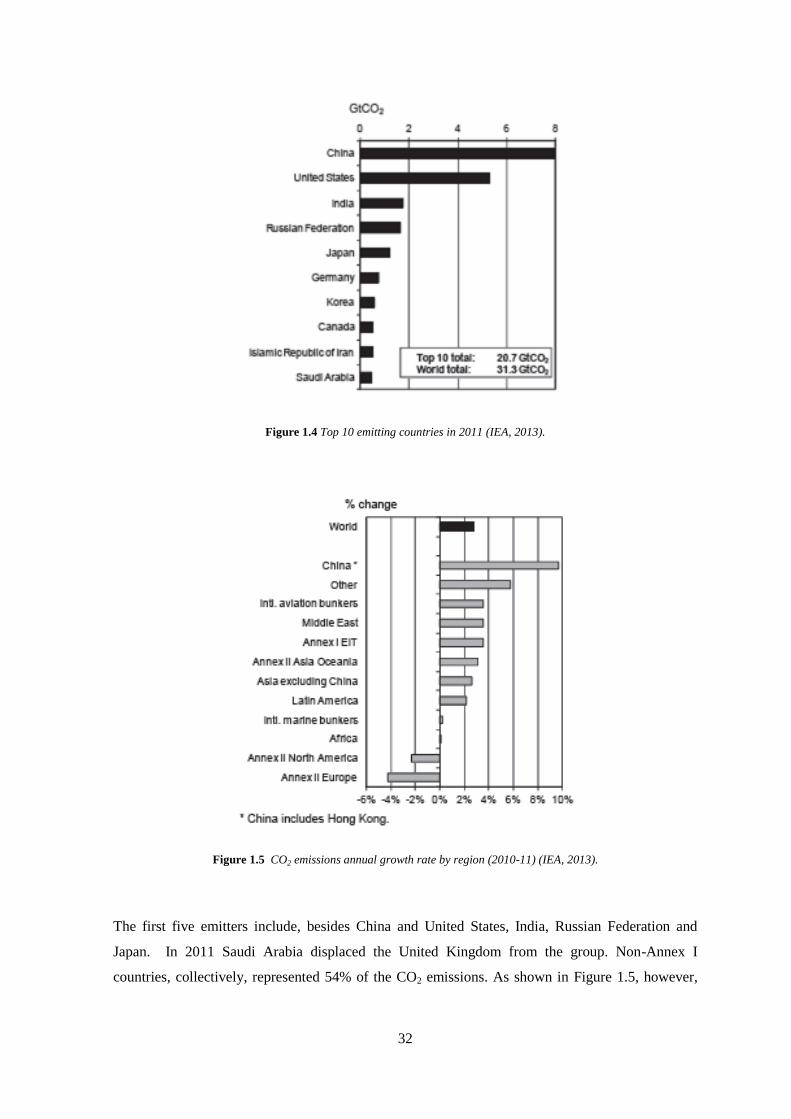
In 2011, nearly two-thirds of global emissions originated from just ten countries, with the shares of
China (25.4%) and the United States (16.9%) far surpassing those of all others. Combined, these
two countries alone produced 13.2 GtCO2 (IEA, 2013). The top-10 emitting countries are shown in
Figure 1.4
Page 36
32
Figure 1.4 Top 10 emitting countries in 2011 (IEA, 2013).
Figure 1.5 CO2 emissions annual growth rate by region (2010-11) (IEA, 2013).
The first five emitters include, besides China and United States, India, Russian Federation and
Japan. In 2011 Saudi Arabia displaced the United Kingdom from the group. Non-Annex I
countries, collectively, represented 54% of the CO2 emissions. As shown in Figure 1.5, however,
Page 37
33
annual growth rates varied greatly: from 2010 to 2011 emissions in China grew strongly (9.7%),
while emissions in Annex II countries decreased (-2.4% in North America and -4.3% in Europe).
Figure 1.6 CO2 emissions per capita by major world regions ( IEA, 2013).
Figure 1.7 CO2 emissions per GDP by major world regions ( IEA, 2013).
Page 38
34
As different countries have largely different economic and demographical situations, these results
would significantly change if considering emissions per capita or per GDP.
Other regions, like the Middle East, Annex II Asia Oceania, Asia and Latin America, experienced
moderate growth (2% to 4%), while emissions in Africa remained stable.For example, among the
three largest emitters, the level of per-capita emissions was 17 tCO2 for the United States, 6 tCO2
for China and 1 tCO2 for India. On average, industrialized countries emit far larger amounts of
CO2 per capita than developing countries. The lowest levels worldwide were those of the Asian and
African region (IEA, 2013). However, as a consequence of their rapidly expanding economies,
between 1990 and 2011 China increased its per-capita emissions by three times and India doubled
them. Conversely, per-capita emissions decreased significantly in both the Russian Federation
(21%) and the United States (13%). Globally, per-capita emissions increased by 14%.
Emissions per unit of GDP were also very variable across regions (Figure 1.7). Although climate,
economic structure and other variables can affect energy use, relatively high values of emissions
per GDP, as for China and Middle East, indicate a potential for decoupling CO2 emissions from
economic growth.
1.2.3 Towards a new international agreement post-Kyoto
With the approval of the Bali Action Plan in 2007 the Parties supported the drafting of a new global
agreement and started the negotiations for the definition of new targets to be achieved after the first
commitment period of the Kyoto Protocol.
The COP15 held in 2009 in Copenhagen had the objective of signing a new international
agreement with reduction targets for the post Kyoto. The European Union proposal was to reduce
the greenhouse gas emissions by 20% compared to the levels of 1990 by 2020 (30% if the other
countries had signed stricter objectives), the United States proposal to reduce the emissions by 17%
by 2020, 42% by 2030 and 83% by 2050 compared to the emissions levels in 2005 (these targets
equal respectively 4% by 2020 and 32% by 2030 compared to the emissions levels in 1990 since
the emissions increased considerably from 1990 to 2005). An agreement was not reached for the
failure in the negotiation between United States and emerging countries like China, India and South
Africa and for the final opposition of some developing countries. At the end of the Conference of
Copenhagen the developed countries agreed to create the Copenhagen Green Climate Fund to
support the development of mitigation projects and policies in developing countries.
A breakthrough in the negotiation post Kyoto was the agreement at the Conference of Durban in
2011, when it was decided that the new global agreement on emissions targets will have to be
achieved by 2015 to come into force by 2020. If agreement can be reached, this will be the first
international climate agreement to extend mitigation obligations to all countries, both developed
and developing. In the mean time the parties signed to extend the Kyoto Protocol, which would
Page 39
35
have ended at the end of 2012, for five more years, to a second commitment period, from 2013 to
2017.
A key challenge in defining the new agreement is that while obligations are to start from 2020,
global emissions need to peak before 2020 if temperature rise is to be limited to below 2°C.
1.3 Renewable energy to mitigate climate change
1.3.1 Greenhouse gas emissions and the energy sector
GHG emissions originate from most human activities, such as transportation, electricity and heat
production, heating, industry, buildings and agriculture. Among human activities the largest
contributor to greenhouse emissions has historically been the energy sector. Based on the
International Energy Agency data, in 2011 the electricity and heat sector accounted for 42% of the
total. Other contributor sectors were: transport 22%, industry 21%, residential 6% and others 9%.
Electricity and heat generation, together with the transport sector produced nearly two thirds of
global CO2 emissions.
Figure 1.8 World CO2 emissions by sector in 2011 (IEA, 2013).
Limiting the analysis to Annex I countries, as shown in Figure, the energy use represented 83% of
the anthropogenic GHG emissions. This percentage varied greatly by country, due to diverse
national structures. Smaller shares corresponded to agriculture, producing mainly CH4 and N2O
from domestic livestock and rice cultivation, and to industrial processes not related to energy,
producing mainly fluorinated gases and N2O (IEA, 2013).
Page 40
36
Generation of electricity and heat are the main cause of greenhouse gas emissions because
worldwide they are heavily relying on fossil fuels.
Figure 1.9 Shares of anthropogenic GHG emissions in Annex I countries, 2011 ( IEA, 2013).
As shown in Figure 1.10 in 2011, fossil sources accounted for 82% of the global total primary
energy supply, oil providing 32% of the world primary energy supply, coal 29%, gas 21% and
other sources, including nuclear, hydro, geothermal solar , tide, wind, biofuels and waste, 18%.
Although coal represented 29% of the world energy supply, it accounted for 44% of the global
CO2 emissions due to its heavy carbon content per unit of energy released. As compared to gas,
coal is nearly twice as emission intensive on average (IEA, 2013). Renewable resources contribute
was only 1% of the whole CO2 emissions, since they are considered carbon neutral.
Figure 1.10 World primary energy supply and CO2 emissions: shares by fuel in 2011 (IEA, 2013).
Page 41
37
As shown in Figure 1.11 the use of coal is responsible of the large majority of CO2 emissions from
electricity and heat generation.
Figure 1.11 CO2 emissions from electricity and heat generation (IEA, 2013).
In some countries, e.g. Australia, China, India, Poland and South Africa over two-thirds of their
electricity and heat is produced through the combustion of coal. Between 2010 and 2011, CO2
emissions from electricity and heat increased by 4.4%, faster than total emissions and CO2
emissions from the combustion of coal increased by 4.9% to 13.7 GtCO2. Coal fills much of the
growing energy demand of those developing countries (e.g. China and India) where energy-
intensive industrial production is growing rapidly and large coal reserves exist with limited
reserves of other energy sources (IEA, 2013).
The situation is worsened by the projections of the world energy demand. With the current energy
policies, the market energy consumption is estimated to increase by 44% from 2006 (497 EJ) to
2030 (715 EJ). The world energy demand expected increase is due to worldwide economic growth
and development. Consequently, CO2 emissions are projected to rise from 29 billion tons in 2006
to 33.1 billion tons in 2015 and 40.4 billion tons in 2030 (corresponding to an increase of 39%)
(IEO, 2009).
The WEO 2013 projections are even worse, stating that by 2035 electricity demand will be almost
70% higher than current demand, driven by rapid growth in population and income in developing
countries.
This growth will cause a progressive depletion of fossil resources and make the availability of
conventional oil and natural gas geographically restricted (Bentley et al., 2007; Hanlon and
McCartney, 2008).
Page 42
38
Furthermore the world energy demand is expected to increase based on the growth trends that have
been registered until now. Between 1971 and 2011, global total primary energy supply more than
doubled (IEA, 2013).
Figure 1.12 World primary energy supply (IEA, 2013).
The increased energy supply mainly relied on fossil fuels. Thus, despite the growth of non-fossil
energy (e.g. nuclear and hydropower), considered as non-emitting, the share of fossil fuels within
the world energy supply is relatively unchanged over the past 40 years. In 2011, fossil sources
accounted for 82% of the global total primary energy supply, versus 86% in 1971.
1.3.2 The promotion of renewable energy and energy efficiency
The Kyoto Protocol contains information about how to reduce the greenhouse gas emissions
suggesting mitigation actions. Among these the role of the energy sector is crucial. The energy
consumption in fact is the first cause of greenhouse gas emissions at global level. Thus the
mitigation actions are mainly focused on the reduction of energy consumption, increase of the
energy efficiency, use of renewable resources and sustainable use of agriculture. In order to achieve
the objectives of the Kyoto Protocol in 2000 the European Union developed the First European
Climate Change Program (ECCP) which identifies a list of priorities and politics to reduce the
greenhouse gas emissions. The actions included the first proposal of a Directive to promote the use
of bio-fuels to produce electricity and heat (combined heat and power bio-fuels). Other measures
included the agricultural and forest sector, particularly the management of forest and agricultural
soils.
The Kyoto Protocol was ratified by the European Union through Decision 2002/358/CE (European
Council, 2002). In particular, the flexible mechanisms proposed by the Kyoto Protocol were
accepted and developed by the European Union. Through the Directive 2003/87/CE the European
Page 43
39
Union Greenhouse Gas Emissions Trading Scheme was established (European Parliament and
Council, 2003a). The Directive requires that, from January 1st 2005 all the energy producers and
the main GHG emitters, obtain an authorization to emit. The authorization is based on National
Plans elaborated by each country to determine the total amount of emission units for each plant. At
the end of the year, those companies that have saved emissions units can sell them in the market to
companies which have emitted more than what was assigned to them.
In 2005 the Second European Climate Change Program was approved, revising and improving the
strategies included in the ECCP I. Through the COM(2008)30 the European Union approved the
2020 Energy and Climate package, which combines the energetic politic with the ambitious target
of greenhouse gas emissions reduction (European Commission, 2008). The European Commission
has pointed out the importance of the contribution of biomass to reach their goals on climate and
energy in 2020. Through the Energy and Climate package, the European Union adopted new
instruments to achieve the following goals by 2020:
- 20% greenhouse gas emissions reduction compared to the 1990 levels (30% if other
industrialized countries will comparably commit and sign an agreement post-Kyoto);
- 20% energy consumption reduction through the improvement of the energy efficiency;
- 20% increase in the production of electricity from renewable sources.
In detail, the package involved the following steps:
- emissions reduction targets for the Member States of the European Union 2020: Decision
406/2009/EC (European Parliament and Council, 2009a);
- new common framework for the promotion of renewable energies: Directive 2009/28/EC ;
- revision of the system of emissions trading for greenhouse gases (ETS) for the post-2012:
Directive 2009/29/EC (European Parliament and Council, 2009b);
- reduction of greenhouse gas emissions in the life cycle of fuels: Directive 2009/30/EC.
The EU Roadmap for a Low Carbon Economy sets a GHG emissions reduction goal of 80% by
2050. The key points of the European Union energy policy are:
- energy saving;
- increased energy production from renewable sources;
- liberalization of the market, eliminating geographical monopolies and giving the possibility
to buyers to choose their supplier;
- integration of GHG reduction targets in the energy policy;
- reduction of the environmental impacts in the energy supply chains;
- security of energy supply;
- low cost of the energy.
The Directive 2009/28/EC on the promotion of renewable energy requires EU member states to
adopt National Action Plans for renewable energy, containing national targets for the share of
Page 44
40
energy from renewable sources consumed in transportation, electricity and heating/cooling in 2020
to ensure that, by that time, an average of 20% of the EU energy consumption comes from
renewable sources (European Parliament and Council, 2009c). Furthermore the Directive sets an
additional national target for the transportation sector, providing that the energy share from
renewable sources in all the forms of transportation will be in 2020 at least 10% of its total national
energy consumption.
The Directive 2009/30/EC on the reduction of greenhouse gas emissions in the life cycle of fuels
sets technical specifications for bio-fuels. Under the directive, the greenhouse gas emissions
produced by the fuel cycle must be reduced by at least 6% by 2020 (European Parliament and
Council, 2009d). The goal, set by the Directive, will be ensured by the prohibition to sale petrol
and diesel fuels with sulfur and additives content higher than the new limits established by the
Directive and the new features that bio-fuels will have to respect. For the production of bio-fuels, in
fact, the use of raw materials that could cause damage to the agriculture and the land use change
which could lead to an irreversible loss of carbon will be prohibited. The Directive applies to road
vehicles, non-road mobile machinery (including inland waterway vessels when not on the sea),
agricultural and forestry tractors and recreational craft.
The Directives 2003/54/EC and 2003/55/EC aim at opening the electricity and the gas market
respectivitely, creating the conditions for effective competition and for the creation of a market
which sets the standards for the production, transport and distribution, licensing, and networks
operation (European Parliament and Council, 2003b, 2003c).
Similarly to the European Union, in 2007 the United States approved a system of economic
incentives to bio-fuels. The Energy Independence and Security Act aims to gradually replace the
use of fossil fuels with biofuels. In order to be eligible for public procurement, it is required that the
overall greenhouse gas emissions of cellulosic bio-fuel produce 60% lower carbon emissions
relative to jet fuel produced from fossil fuel (U.S. Government, 2007).
Al national level, Italy has been implementing a series of politics to reduce greenhouse gas
emissions in compliance to international and European legislation. Through the Law n.120 of June
1st, 2002 Italy ratified the Kyoto Protocol, according to whom it is committed to reduce greenhouse
gas emissions by its national reduction target of 6.5% compared to the 1990 levels (Parlamento
Italiano, 2002). With CIPE "Resolution of 19/12/2002, Italy adopted a National Plan for the
Emissions Reduction (CIPE, 2002). The mitigation actions in accordance with the Kyoto Protocol
include the improvement of the energy efficiency and use of renewable energy in relevant sectors
of the national economy, the protection and improvement of carbon sinks and stocks, promotion of
sustainable forest management practices, afforestation and reforestation the promotion of advanced
and innovative green technologies and the adoption of fiscal incentives to reduce GHG emissions.
Page 45
41
The Directive 2003/87/EC has been transposed into national law through the Legislative Decree
216/2006. The decree identifies the procedure which leads to the approval of the National
Allocation Plan for renewable energy in Italy (NAP) and establishes the emissions and the emission
shares National Registry.
The Legislative Decree 28/2011 implemented the Directive 2009/28/EC on the promotion of
renewable energy, which sets binding targets for each Member State, consistent with the overall
objective of the EU gross final consumption of at least 20% in 2020 (Consiglio dei Ministri,
2011a). For Italy, the objective is a share of not less than 17% of final energy consumption from
renewable sources. To achieve the goal the decree improves the incentives system for the
production of energy from renewable sources (electricity, thermal energy, bio-fuels) and for the
increase of energy efficiency.
The Directive 2009/30/EC was implemented by Legislative Decree No. 55/2011 on the reduction
of greenhouse gas emissions in the life cycle of the bio-fuels. The Decree defines the criteria for the
environmental sustainability of bio-fuels (and bio-liquids) necessary in order to make them
countable for achieving the national targets on renewable energy (Consiglio dei Ministri, 2011b).
1.3.3 Incentives systems to the bio-energy production
1.3.3.1 The White Certificates or Energy Efficiency Certificates
To promote renewable energy production and energy saving, the EU energy policy includes
incentive systems to the, through the White and Green Certificates systems.
White Certificates are generated from energy saving measures evaluated based on a mandatory
obligation. Subjects who saved more than the obligation target could sell those energy saves as
“white certificates” to some other subjects to meet their energy saving goals.
In Italy the incentives system is managed by the Electrical Service Manager (GSE) and the Energy
Market Manager (GME). The GSE role is to promote the development of renewable energy
through the green and white certificates. The GME is responsible for the organization and
management of the green and white certificates, the emission allowances and the energy market
power exchange (IPEX Italian Power Exchange).
The Authority for the Electricity and Gas establishes the requirements for the major electricity and
natural gas distributors to obtained certified energy savings. Energy Efficiency Certificates
corresponding to the certified savings are issued by the Energy Market Manager to the project
implementing body measured in terms of TEEs, which corresponds to 1 tep (ton of equivalent
petrol) of saved energy and is valid for five years.
Page 46
42
Subjects may decide to carry out energy efficiency actions or to buy white certificates. The price is
set by the market and 1 toe corresponds to around 11628 kWh of fuels, 5347.59 kWh of electricity
consumption. Certificates are of three types:
- Type I: reduction of final consumption of electricity;
- Type II: reduction of natural gas consumption;
- Type III: interventions other than the two above.
Types of interventions that are eligible to acquire TEE (they can be aggregated into a single
project):
- photovoltaic plant with power <20 kWp;
- double glazing;
- high-efficiency gas boiler;
- district heating and domestic hot water production;
- small cogeneration systems for winter heating, summer cooling and hot water production;
- recovery of electricity from natural gas decompression;
- break jet taps;
- replacing light bulbs with energy saving bulbs;
- replacement of electric water heaters with natural gas water heater with sealed chamber.
Eligible entities to obtain TEEs include:
- electricity and natural gas distributors;
- companies controlled by the distributors;
- companies operating in the energy services (ESCO):
- subjects with mandatory energy manager.
ESCOs are companies which finance, develop, install projects to improve energy efficiency so that
the saved energy is worth enough to repay the cost of investment.
The customer does not pay at the time of construction, costs are covered by the ESCO which
obtains loan at favorable interest rates. The nature of the contract between the ESCO and the
customer is associative: the customer receives free energy for e.g. 20 years, leaving the incentives
of the energy bill to the ESCO; the customer becomes owner of the system after 20 years while the
initial risk of the project is entirely assumed by the ESCO.
1.3.3.2 The Green Certificates
Green Certificates are generated from increasing the share of energy produced from renewable
sources compared to a mandatory obligation. Subjects who produced a larger share of energy from
renewable sources than the mandatory target, could sell the corresponding “green certificates” in
the energy market.
Page 47
43
In Italy in 1999 the Bersani Decree replaced the CIP 6 system with the Green Certificates
(Consiglio dei Ministri, 1999). The eligible plants included:
- plants powered by renewable sources, including hybrids, entered into operation after April
1st 1999 as a result of new construction, expansion, renovation of all or part of them;
- co-combustion plants (hybrid plants);
- cogeneration plants combined with district heating which satisfy the conditions foreseen in
the Ministerial Decree 18/12/2008 (Ministero dello Sviluppo Economico, 2008).
The requirement for electricity producers from fossil fuels was to produce a percentage of
electricity from renewable sources: they can either do it independently or buy green certificates.
A green certificate corresponded to 1 MWh produced from renewable sources. The value of green
certificates was added to the fare of the energy sold in the network, which varied depending on
certain energy intervals. The green certificates thus doubled the value of a system which used
renewable sources compared to a traditional one which uses fossil fuels.
The period entitled to receive green certificates:
- 15 years for plants using renewable sources and for thermal power plants entered into
operation before April 1st, 1999 and that, after December 31st, 2007, began to operate as
hybrid power plants:
- 12 years for plants using renewable sources entered into operation before December 31st,
2007, and for thermal power plants which entered into operation began operating before
April 1st, 1999, which began to function as a hybrid plants before December 31
st, 2007
- 8 years for non-incentivized electricity from renewable sources in cogeneration plants
combined with district heating and also hybrid-powered plants from non-biodegradable
waste that entered into operation by December 31st , 2006.
1.3.3.3 All-inclusive fare
In case of small renewable energy plants an all-inclusive fare is used as a form of incentive for each
kWh produced and for each kWh sold.
On request of the manufacturer, for plants entered into operation after December 31st , 2007, with
average nominal annual power not exceeding 1 MW and 0.2 MW for wind plants, the net energy
can be incentivized, in alternative to the green certificates, through an all-inclusive fare, variable
depending on the source, for a period of 15 years.
Eligible plants include:
- wind plants for power <0.2 MW;
- geothermal;
- wave;
Page 48
44
- hydraulic plant different from the previous one;
- biogas and biomass;
- landfill gas, from sewage treatment plant and liquid bio-fuels.
The all inclusive fare can change every 3 years. Only one transition from green certificates to fixed
rate or vice versa is possible.
The Romani Decree n.28 of 2011 introduced large modifications in the incentives system for plants
commissioned after December 31st 2012 which include:
- linear reduction of the mandatory portion that will cancel in 2015;
- the import will not be subject to obligation since 2012;
- expected cut the value of the green certificates that affects retroactively existing
installations;
- the all-inclusive tariffs will remain fixed for the duration of the incentive.
Specific incentives for:
- bio-methane used in high yield (80%) cogeneration plants for the electricity production;
- biogas biomass, bio-liquids installations, into operation after December 31st, 2012,
combined with other government incentives in the case of cogeneration plants and
regenerative powered by solar or biomass or biogas.
1.4 The use of wood for bio-energy
As described above, the use of bio-energy is considered to be crucial to fight climate change. The
energy sector, in fact, is the dominant contributor to global warming because of the current large
use of fossil fuels for energy production which is responsible of the release of big quantities of
greenhouse gas emissions to the atmosphere.
To reduce greenhouse gas emissions legislation and incentives systems have been introduced to
promote and diffuse the use of renewable energy. Worldwide bioenergy provides today only 10%
of the world’s total primary energy supply and most of this is used in the residential sector for
heating and cooking purposes (GBEP, 2007).
Among different ways of producing renewable energy, biomass is largely used. The term
"biomass" refers to organic matter that has stored energy through the process of photosynthesis.
The chemical material (organic compounds of carbons) are stored and can then be used to generate
energy. Common examples of biomass include food crops, crops for energy (e.g., switchgrass or
prairie perennials), crop residues (e.g., corn stover), wood waste and byproducts (both mill residues
and traditionally noncommercial biomass in the woods), and animal manure (Bracmort and Gorte,
2009). Among those wood represents one of the most promising biomass source. Wood has been
the first fuel historically adopted before being replaced by fossil fuels. In developing countries
Page 49
45
traditional bioenergy use (fuelwood and charcoal) still dominates since up to 95% of national
energy consumption relies on biomass (Cherubini et al., 2009).
Wood is largely available worldwide and, if correctly managed through a sustainable management,
can represent un unlimited source.
Figure 1.13 Representation of the carbon cycle.
As shown in Figure 1.13 wood, as renewable resource, is part of the natural carbon cycle. Carbon is
converted and stored in woody biomass through photosynthesis. Humans interferee with the natural
carbon cycle by harvesting, processing, transporting and using the wood material. When wood is
harvested carbon is transferred from one carbon pool (standing forest) to another (harvested wood
product). Harvested wood can have different destinations:it can be used either to produce bio-
energy or long lasting products or products for the paper industry.
When burned to produce bio-energy the carbon content is released back to the atmosphere during
combustion. Forest operations of cutting, chipping and transporting wood as well as the
manufacture of wood products release greenhouse gas emissions which depend on the technology
adopted.
1.5 The environmental sustainability of woody biomass bio-energy
1.5.1 Life Cycle Assessment (LCA)
The use of woody biomass for energy production is part of the strategy to reduce the global
greenhouse gas emissions. Since wood is one of the oldest fuel used for energy production, several
Page 50
46
methodologies have been developed during the years to evaluate its sustainability. Some of them
have been abandoned, most of them still coexist.
Biomass energy is often considered for its potential of mitigate climate change, so global warming
is the focal indicator for bio-energy considerations. However more recent methods consider the
sustainability from a wider point of view, expanding the system boundaries to the whole life cycle
of the product and considering a larger set of impact categories.
An overview of the evaluation methodologies is presented, adopted both in international politics
and on voluntary level. They can be classified in two main approaches:
- I approach limited to direct emissions;
- II approach: life cycle approach.
The first approach started in the ‘80s and is still present in most of the regulations for the mitigation
of climate change. It consists in evaluating the environmental impacts of biomass, based on the
direct emissions released in atmosphere by its combustion, assumed to be equal to carbon
absorption in forest. This method is used in the Kyoto Protocol and described in the IPCC
Guidelines (IPCC, 2006) which include specific evaluation methods for each activity sector. In this
approach different stages of the biomass life cycle are accounted separately.
In the Kyoto Protocol the forestry sector is accounted through art.3.3 (afforestation, reforestation
and deforestation) and art.3.4 (forest management). Through the carbon stock method the increase
in biomass growth in forest is accounted as a negative emissions and reported in the National
Inventories for the GHGs to offset the emissions.
The harvesting activity on the contrary is assumed to be an instantly release of carbon dioxide to
the atmosphere based on the default assumption that all the carbon dioxide stored in the wood in
forest is instantly emitted into the atmosphere after harvesting. This assumption is like considering
that all the harvested wood is instantly burned.
For the first commitment period of the Kyoto Protocol (2008-2012) no distinction was made
between wood products for bioenergy and long lasting wood products, since the harvesting activity
was accounted as an instant carbon dioxide emission, not considering that the carbon could be
stored in long lasting wood products for decades as carbon stock.
However the 2006 IPCC for Harvested Wood Products recognized the role of carbon stocks in
wood products and its methodological framework and their introduction in the emissions
accounting has been much discussed in the negotiations for the post-Kyoto. They have been
recenty introduced in the accounting for the GHG Inventories for the Kyoto Protocol after the
conference of parties in Durban. Based on the IPCC Guidelines, the energy produced from woody
biomass is consider to have an emission factor equal to zero. This statement is based on the
assumption that all the carbon stored in biomass is instantly released during combustion as carbon
Page 51
47
dioxide and that the carbon dioxide released equals the carbon dioxide that was absorbed from the
atmosphere for the biomass growth.
Given the importance of the Kyoto Protocol at international level, most of the subsequent
international legislations for the mitigation of climate change adopted the same approach.
Also on voluntary level, many standards for the evaluation of the environmental sustainability of
woody biomass bioenergy are based on this assumption.
The second approach is called “life cycle assessment” (LCA). This approach is relatively recent,
since it began to be adopted as voluntary tool at the beginning of 2000. Life cycle assessment is
defined as the “Compilation and evaluation of the inputs, outputs and the potential environmental
impacts of a product system throughout its life cycle”. It is a global approach which aims to
evaluate the overall impact of a product from the acquisition of the raw materials from the
environment, until the end of life, considering all the phases of transportation, forest operations and
wood processing needed to manufacture the final product and distribution of the product to the end
users. The LCA approach recognizes the importance of expanding the system boundaries going
beyond the calculation to the whole supply chain to identify the most critical stages and define a
real reduction strategy acting where it is more effective and economically viable.
The LCA calculation can be performed according to one of the following approaches:
- From cradle to grave: it takes into account the environmental impacts throughout the entire
life cycle from the acquisition of the raw materials and natural resources from the
environment to the production phase, the distribution phase until the final disposal;
- From cradle-to-gate: it takes into account the environmetal impacts from the acquisition of
the raw materials from the environment until the product manufacture, including all the
upstream emissions.
- From gate-to-gate: it takes into account the enviormnental impacts for the product
manufacture.
LCA is constituted by the following four phases:
- Goal and scope definition
- Life cycle inventory analysis (LCI)
- Life cycle impact assessment (LCIA)
- Life cycle interpretation.
In the LCA framework, the evaluation of the greenhouse gas emissions with life cycle approach is
called Carbon Footprint. LCA does not limit the evaluation to global warming, but it includes many
othe impact categories on both local and global scale, for air, water and soil compartments, e.g.
stratospheric ozone depletion, human toxicity, acidification, eutrophication, eco-toxicity,
photochemical ozone creation potential (POCP), land use , depletion of abiotic resources, habitat
and ecosystems. However, as discussed above, the impact on global warming is a key indicator to
Page 52
48
evaluate the bioenergy sustainability. The LCA methodology will be described in detail in Chapter
3 of this dissertation.
1.5.1.1 International LCA programs and standards
Life Cycle Assessment is performed based on internationally recognized approaches. The
international standards for Life Cycle Assessment are ISO 14040 and ISO 14044. In 2013 the ISO
published ISO 14067, a specific standard for the quantification and reporting of the carbon
footprint of products (ISO, 2013a).
For the evaluation of the emissions at organization level currently the most common international
standard is the ISO 14064 (ISO, 2006c). This standard specifies requirements for measuring,
monitoring, reporting and verifying the greenhouse gas emissions and removals within the
organization system boundaries, establishing that the accounting is mandatory for the emissions of
the first two categories (direct and indirect from energy consumption) and optional for the third
category (other indirect). In 2013 the ISO published the ISO 14069, which represents a guideline
for the application of ISO 14064 (ISO, 2013b). Another widely used standard for the calculation of
the greenhouse gas emissions at organization level is the GHG Protocol, developed the World
Resources Institute (WRI) and the World Business Council for Sustainable Development
(WBCSD). This approach provides a detailed guide, freely accessible online for the compilation
and reporting of the emissions of organization. The wide adoption of this standard is attributable to
the inclusion of many stakeholders in its development.
In 2011 the GHG Protocol published a specific document on the Corporate scope 3 (value chain)
accounting and reporting (WRI and WBCSD, 2013), which contains information on how to
calculate the indirect emissions of the organization to understand, manage and report the GHG
emissions throughout the supply chain.
In line with the ISO standards the European Commission Joint Research Centre, within the
European Platform on Life Cycle Assessment (EPLCA), developed the ILCD handbook, consisting
of a set of documents including a general guide for LCA and a specific guide for LCI data sets
builds on the general guide, which provides more detail for the generation of specific types of data
(European Commission, 2010). Specific technical documents have been developed for the Carbon
Footprint, both at product and at organization levels.
In the last years, several programs have been developed at international level for the calculation
and management of the environmental performances of products at voluntary level.
Since 2001, the United Kingdom has implemented a program with the Carbon Trust to calculate,
reduce and report the greenhouse gas emissions, contributing to provide technical expertise for the
development of one the most spread international standard, the PAS 2050. The PAS 2050 (BSI,
Page 53
49
2011), developed by Carbon Trust, Defra and the British Standards Institute (BSI), includes
specific requirements regarding the definition of the objectives, the inventory analysis, the
identification of the system boundaries and the temporal aspects of the GHG emissions, clarifying
the approach that should be considered by the organizations that implement the Carbon Footprint
and simplifying procedures of LCA focusing on the emissions of greenhouse gases. The PAS,
while basing its roots on the methodology of Life Cycle Assessment, clarifies important issues
providing a rigorous and practical approach for the carbon footprint. In Germany from 2007 to
2009 the PCF Project was carried out to promote the emissions reduction along the supply chain.
Furthermore Germany developed a label system called Blue Angel, which applies to goods and
services that have, based on a life cycle approach, less impact than the market average.
One of the most ambitious program was undertaken by France in 2009, through the Grenelle Law,
which launched a project for the quantification of the environmental impacts and the
communication of the results to the end users. The goal was to test different aspects e.g. evaluation
methods, data sources, communication methods, consumers response, cost, impact on business. At
the same time the Ademe-Afnor platform developed a general methodology to calculate the
environmental impacts of products to produce Product Category Rules and to build a public
database for the life cycle of products. The law aimed to make mandatory the diffusion of the
information about significant environmental aspects, such as the greenhouse gas emissions, water
and resources consumption, impact on biodiversity, through environmental labels applied on
products. Thus the consumer will be able to compare and choose the products to buy, also based
on sustainability criteria.
Programs for the calculation and reporting of the carbon footprint of the products have also been
growing in Sweden, with the International EPD system and the Climate Certification of food chain,
a Swedish initiative to assess the impact on climate change in the food sector developed from the
EPD label (ISO, 2006d), in Switzerland with the Climatop labeling, Intelligent Labelling, Climate
Frendly Products and in Austria with the Zurück zum Ursprung labeling system.
Also in Asia programs for the calculation and labeling of the carbon footprint are becoming more
common: in Korea, after a 9-month pilot program, in February 2009 the Environmental
Technology Institute of Korea (KEITI) introduced the Carbon Footprint Label. Since then, more
than 400 products and services have been labeled. In Japan, the Ministry of Economy, Trade and
Industry, in response to a Action Plan for a Low Carbon Society in 2009 launched a project for the
Product Carbon Footprint (CFP) based on the ISO 14040- 44 and ISO 14025. The pilot project took
three years and produced important results in terms of number of tested products, database
produced and educational events organized. At the end of the pilot project the Japanese Association
for the Environmental Management for the Industry (JEMAI) launched a program in April 2012 for
the CFP Communication, which was be carried out based on the results obtained in the previous
Page 54
50
three years. The goal was to give visibility to the CFP, to reduce the cost and to include a greater
number of stakeholders.
Also Taiwan, Thailand and Nigeria have developed systems for the calculation and labeling of the
product Carbon Footiprint, respectively the Taiwan Carbon Footprint Labels, the Thai Carbon
Footprint and Labelling Initiative and the Lagos State Carbon Footprint and Management Project
and a pilot project started by the government in Quebec, the Carbon Footprint of Products
Labelling Pilot Project from the Quebec Government.
Italy has also recently launched projects for the calculation of the environmental impacts in many
productive sectors. In 2011, the Ministry of Environment allocated funding to perform studies on
the carbon footprint by selecting companies operating in different sectors related to consumer
goods, creating a working group whose goal was to develop and test methodologies for the
calculation of sector carbon footprint.
1.6 State of the art of LCA of wood products for bioenergy
1.6.1 Research projects about the evaluation of the environmental impacts of wood
products
As far as the forestry sector is concerned, there are major initiatives in the international scene. One
of these is the establishment in 1996 of the Consortium for Research on Renewable Materials
Industry (CORRIM) from 15 research institutes to conduct research on the use of wood as a
renewable material. CORRIM published a research plan containing twenty-two modules to develop
a life cycle assessment (LCA) about the use of wood for residential and for other uses. The research
plan led to the creation of a comprehensive inventory of inputs and outputs of the environmental
life cycle of timber products from the forest management to the final product, including its
manufacture, use, maintenance and disposal. The results of the first phase of the program are
published in a summary report (CORRIM, 2001).
CORRIM is one of the largest LCA organizations in North America over the last decade it has
developed research protocols in compliance with the ISO standards for the life cycle inventory
(LCI) for the measurement of all inputs and outputs for each processing stage, including forest
management, harvesting, transportation, woodworking, manufacturing, maintenance and use, until
the final disposal, producing databases that allow to quantify the emissions from the forest to the
post-consumption, evaluating the emissions from a carbon pool to another and measuring the
interactions between them.
The research has highlighted the impact of the management and policies on greenhouse gas
emissions on the different carbon pools for the major supply regions in the United States (Bowyer
et al., 2004; Perez-Garcia et al., 2005). The studies carried out by CORRIM represent an important
Page 55
51
source of information for the purposes of this study.
At European level, the European Confederation of Woodworking Industries (CEI-Bois), the
Confederation of European Forest Owners (CEPF) and the Confederation of European Paper
Industries (CEPI) have created a technology platform for the forestry sector, the Forest Technology
Platform (FTP) (http://www.forestplatform.org/). The Forest Technology Platform is led by
industry to establish and implement a roadmap for research and development for the sector, and is
supported by a large group of stakeholders. The FTP has developed a Vision 2030 for the wood
sector, which defines as main objective to develop research and knowledge to make the forest
sector competitive and promote the use of renewable forestry resources.
The work of the FTP was performed under the Seventh Programme Framework of the European
Commission (2007-2013). The technology platforms are the main 'channels' to give specific inputs
to work programs and for the cooperation with the European Commission in the specific area.
The main research priorities of the Platform were included in the Platform Strategic Research
Agenda (SRA), the first research program that integrates all of the major networks in Europe and
industrial initiatives in the forestry sector in a geographically balanced way.
Another European research project, Eforwood, aimed to develop mechanisms for evaluating the
contribution of wood to the sustainable development. The project covered the entire European
forestry supply chain from the production to the consumption and recycling of materials and
products. Eforwood was the first project funded by the European Commission which covers the
whole European forest sector.
1.6.2 Literary review about LCA of woody biomass bio-energy
After analyzing the international mandatory regulations and voluntary programs framework, the
scientific liteture about Life Cycle Assessment of woody biomass bio-energy has been reviewed.
75 papers have been analyzed, 6 of them were already reviews (Cherubini, 2010; Cherubini et al.,
2009; Cherubini and Strømman, 2011; Heinimann, 2012; Helin et al., 2013; Kloepffer, 2008).
Some of the analyzed papers dealt with the LCA of wood products for building constructions
(Bergman and Bowe, 2010; Hubbard and Bowe, 2010; Lippke et al., 2011a, 2010; Perez-Garcia et
al., 2005; Puettmann et al., 2010a, 2010b; Wilson, 2010a, 2010b, 2010c) but were still included in
the review since they provided a lot of data about forest operations from the CORRIM database.
The topics addressed in the reviewed papers, the first author’s organization country and the year of
publication are shown in Figure 1.14 and Figure 1.15
Page 56
52
Figure 1.14 Ripartition of the topic addressed in the review papers.
Figure 1.15 Ripartition of the first author’s organization countries of the review papers.
The majority of the review papers were LCA studies (38.67%). Papers about forest management
and climate change also represented a large share of the total (17.33%) and some papers about
dynamic LCAs (14.67),.harvested wood products (9.33%), reviews (8%) and others (12%)
including fires management, carbon stocks, biogenic carbon and time horizon were analized.
Regarding the origin of the reviewed papers, since co-authors from different contries are often
involved, the first author’s organization contries were considered for comparison. The large
majority of the reviewed paper were from the United States (36.49%). Many reviewed studies, in
fact, were carried out within CORRIM. A quite large number of studies came from Scandinavian
countries (Finaland, Sweden and Norway) which overall accounted for 28.38%. The remaining EU
countries accounted for 21.62%. In total 50% of the analyzed papers were from EU and 44.59%
Page 57
53
from United States and Canada. The remaining 5.41% included papers from Australia, Brazil,
Japan and China.
Figure 1.16 Ripartition of the years of publication of the review papers.
More than three quarters of the reviewed papers (78.38%) were published from 2008 to 2014, in
same percentage (39.19%) for the two periods 2008-2010 and 2011-2014. The remaining 21.62%
of the papers were published between 1996 and 2008.
The results of the review are presented in the following paragraphs. The key aspects outlined are
described in the following paragraphs and regard the following aspects: case studies and data
availability; environmental benefits of replacing fossil fuels with bio-energy; carbon neutrality;
harvesting, conversion and distribution phases; forest management and dynamic LCA.
1.6.2.1 Case studies and data availability
Cherubini and Strømman reviewed the state of the art of life cycle assessment of bio-energy
systems, both as transportation fuel (bio-ethanol and bio-diesel) and for heat and power production
(Cherubini and Strømman, 2011). They found that the majority of the analyzed papers focused on
bio-ethanol and bio-diesel production. The number of studies evaluating the environmental
performances of biomass for heat and power production was slightly lower than that for
transportation bio-fuels. The authors justified the result by observing that, while electricity and heat
can be produced by a variety of renewable sources (wind, solar, hydro, biomass, etc.), the only
alternative to fossil resources for production of fuels and chemicals is biomass.
The Life Cycle Assessment approach is not limited to the global warming impact category.
Although almost the totality of the reviewed studies included Global Warming Potential in the
evaluation, some LCA studies have also examined life cycle impacts on other environmental
categories, including local air pollution, acidification, eutrophication, ozone depletion, land
use(Merra et al., 2001).
Page 58
54
Moreover it has emerged that there is heterogeneity in the evaluation methods, regarding the use of
different indicators, system boundaries, allocation procedures (Merra et al., 2001), functional units
and reference systems. This means that outcomes are often not immediately comparable and of
difficult interpretation.
This highlights a critical limit of LCA studies recognized by the ISO 14040, which is that LCA
only addresses the environmental issues that are specified in the goal and scope of the study.
Therefore, it is not a complete assessment of all environmental issues of the product system under
study.
Furthermore, one of the limitation outlined by the ISO 14040, is the lack of availability of collected
inventory data appropriate and representative for each impact category. Moreover, the LCI data
available are often evaluated as global or European average values. From the literary review, it
emerged that a small number of Italian case studies about this topic exist (Cespi et al., 2014;
Valente et al., 2011). Critical issues outlined by the ISO are also associated with the limited
development of characterization models, inadequate LCI data quality which may, for instance, be
caused by uncertainties or differences in allocation and aggregation procedures.
1.6.2.2 Environmental benefits of replacing fossil fuels with bio-energy
The large majority of the reviewed studies highlighted the environmental benefits deriving from
replacing fossil fuels with bio-energy from renewable biomass sources, which, according to
Cherubini and Strømman, represent the main driving forcing for promoting the production and use
of bio-energy (Cherubini and Strømman, 2011).
Producing cellulosic bio-fuels from wood resources that are currently wasted or are not of adequate
quality for other uses can substantially reduce emissions by substituting fossil fuels that have a
disproportionately larger impact (Lippke et al., 2012; Pingoud et al., 2010).
It was highlighted that the benefits of using wood-based energy are multiple and include not only
emissions reduction from the combustion of fossil fuels, but also the utilization of locally available
raw materials and to some extent, the reduction of carbon emissions owing to the decomposition of
forest residues left after final felling (Alam et al., 2010).
Several studies have demonstrated the overall benefit for the environmental associated with the use
of wood instead of traditional fossil fuels such as coal and natural gas (Cherubini et al., 2009;
Lippke et al., 2011a; Sathre and Gustavsson, 2012; Sathre and O’Connor, 2010).
A recent study of Puettmann and Lippke simulated different fuel-substitution scenarios and proved
that all of them resulted in a decreased GWP. Moreover it was shown that larger benefits were
obtained producing heat instead of electricity, since using woody biofuel for electricity production
Page 59
55
was somewhat less effective in lowering carbon emissions than when it was used for heat energy
(Puettmann and Lippke, 2012).
Reed et al., 2012 analyzed the fossil emission reduction when combusting pellets compared with
natural gas and found that the reduction varied from 123% to 56% based on the type of allocation
adopted.
Emission reductions were also estimated on a country level. A recent study evaluated the net
emission reductions in Japan between 2005 and 2050 through the massive use of wood resources
for energy (Kayo et al., 2011).
However, a key issue emerged by the analysis of studies about the emission reduction deriving by
the use of bio-energy: the resulting GHG emissions savings are largely variable with the fossil
reference system considered. For example, if electricity in the fossil reference system is produced
from natural gas, this option has a GHG emission factor of 120 g CO2-eq./MJ. By contrast, if it is
produced from coal, the GHG emission factor is 237 g CO2-eq./MJ. Thus for the comparison the
definition of the fossil reference system has a strong importance (Cherubini, 2010).
1.6.2.3 Carbon neutrality
The evaluation of the environmental benefits in terms of emission reduction deriving by replacing
fossil fuels with bio-energy is based on some methodological assumptions.
There is a primary distinction between fossil fuel and biofuel CO2 emissions which is related to the
source of the carbon stored in them. The use of fossil fuels releases geologic carbon that has been
stored in the ground, and those emissions represent a net addition of CO2 to the atmosphere (fossil
fuel-derived CO2 emissions). Bio-energy uses wood or wood residue derived from timber harvest
operations. Trees sequester atmospheric carbon dioxide as they grow and burning biofuels simply
releases this sequestered carbon dioxide back into the environment (biogenic CO2 emissions)
(Bergman and Bowe, 2010). With a sustainable forest management, where removals plus
decomposition of dead and dying residuals do not exceed growth from one rotation to the next, the
net addition of CO2 into the atmosphere will be null and the forest will remain carbon neutral
(Lippke et al., 2010).
The PAS 2050:2011 defines “fossil emissions” as those that are released through the combustion or
decomposition of fossilized material (e.g., coal, oil and natural gas), “biogenic emissions” as those
that are released through combustion or decomposition of biomass (i.e., material of biological
origin) (BSI, 2011).
Based on the International Reference Life Cycle Data System (ILCD) Handbook (European
Commission, 2010) and the EPA accounting framework (EPA, 2011), the impact on global
warming is entirely attributed to fossil GHG emissions while biogenic emissions are considered to
Page 60
56
be carbon neutral and are not reported in the LCA indicators.
As in the Kyoto Protocol approach, in the LCA approach the impact of bio-energy on global
warming is based on the carbon neutrality assumption, based on the idea that the release of carbon
dioxide during the conversion of biomass to energy is balanced by the carbon sequestered within
that biomass.
In carbon accounting terms, carbon sequestration during biomass growth is accounted for as a
negative emission. The net GHG emissions from biologically based energy products is evaluated
by subtracting the amount of CO2 taken up during biomass growth in the first stage of the product
life cycle from the amount of CO2 (including biogenic) released to the atmosphere during all life
cycle stages of the product (Brandão et al., 2013). Among the new and developing approaches, the
ISO 14067 (ISO, 2013a) and GHG Protocol (WRI and WBCSD, 2013), as well as the revised
Publicly Available Specification (BSI, 2011), require that the biogenic contribution be excluded
from the accounting although it may be calculated and reported separately.
The analysis of the scientific literature on the Life Cycle Assessment shows that, in most of the
cases, as far as the global warming is concerned, biomass is considered to be carbon neutral
(Cherubini et al., 2009; Helin et al., 2013; Hubbard and Bowe, 2010; Katers et al., 2012; Lippke et
al., 2011b, 2010; McKechnie et al., 2011; McManus, 2010; Oneil et al., 2010; Oneil and Lippke,
2010; Routa et al., 2012a, 2012b; Werner et al., 2010; Whittaker et al., 2011; Wilson, 2010a,
2010b, 2010c).
The assumption of carbon neutrality:
- in the Kyoto Protocol approach simply attributes an impact on global warming equal to
zero ignoring the emissions generated in other processes associated with the wood products
supply chain;
- in the LCA approach the impact on global warming of the combustion is assumed to be
equal to the benefit of carbon sequestration and the net impact is associated with the
remaining phases of the life cycle.
The assumption of carbon neutrality has been widely adopted although it has been recognized that
in some cases (i.e. in presence of catastrophic wildfire or pathogen outbreaks) this assumption
needs to be examined in greater detail because forest carbon may deviate substantially from a
sustainable management regime (Oneil and Lippke, 2010).
Considering the combustion of wood fuel as carbon-neutral in this manner is consistent with many
groups overseeing environmental concerns (BSI, 2008; EPA, 2003; IPCC, 2013; Wilson, 2010a,
2010b). Furthermore the CORRIM research protocol treats forests under sustainable management
as carbon neutral (Oneil et al., 2010).
Based on the carbon neutrality assumption, when biomass is combusted the resulting CO2 emission
is not accounted for as a GHG because C has a biological origin and combustion of biomass
Page 61
57
releases almost the same amount of CO2 as was captured by the plant during its growth. However,
combustion reactions cause emissions of other GHGs like N2O and CH4, which must be estimated
and accounted for in the GHG balance (even if their contribution is expected to be small).
Furthermore, some studies have shown that, given the large quantities of pollutants released,
combustion can have a high impact on photochemical smog and human toxicity (Cespi et al., 2014;
Solli et al., 2009).
1.6.2.4 Harvesting, conversion and distribution phases
The environmental impacts of bio-energy are not only associated with the combustion phase but
also with other phases of the LCA, including forest operation, logistics and distribution of the final
product. The conversion of forest residuals to bio-energy requires various inputs from nature (the
atmosphere) and industry (the technosphere). Hence, the overall environmental footprint associated
with the production of bio-energy includes all the resources used, emissions and waste generated
during the process of biomass growth, collection and conversion into biofuel. All these processes
require energy, both heat (supplied with natural gas or oil) and electricity (usually taken from the
grid), which results in GHG emissions which usually have a significant influence in the final
balance (Cherubini, 2010).
There are some studies carried out in the 90’s about the environmental impacts of forest operations.
One of these evaluated the GHGs emissions due to use of primary energy in silvicultural and
forest-improvement work, wood harvesting, and timber transportation in Finland (Karjalainen and
Asikainen, 1996). The study showed that silvicultural and forest-improvement work caused smaller
emissions than did timber cutting, haulage or long-distance transportation.
Another study about the environmental impacts of forest operations compared two different types
of forest management: the first was a clear cutting and shelterwood cutting in forest-management
systems based on even-aged management; and the second one included mechanized and
motormanual operations for felling and bucking. It was found that final felling in the form of
creation and removal of shelterwood gave rise to higher emissions of CO2 and NO if compared
with clear cutting. The explanation that the author gave was that the shelterwood system involves
felling in several stages, with productivity in each stage being lower than in clear cutting (Berg,
1997).
Harvesting operations include a large number of equipments and many sets of different forest
operations based on the characteristics of the area to harvest.
As a consequence of different log size, different transport distances in the forest, and, in particular,
different transport distances from the pile to the factory, there are also large variations in emissions
from forestry operations (Michelsen et al., 2008).
Page 62
58
Biomass is subject to transportation in many points of the supply chain, within the supply chain or
to the final users, by means of suitable transport means (e.g. trucks, ships, rails). From the literary
review, contrasting conclusions have been reached about the impact of transportation on the whole
life cycle assessment of bio-energy. According to Cherubini et al., 2010 this step usually has a
small influence in the GHG balance if the fuel is used within a range of 200–300 km, while it may
become relevant if a transoceanic boat transport takes place.
Conversely, another study asserted that transport was one the major energy-consuming sectors and
thus a significant source of carbon dioxide emissions in the bio-energy balance (Karjalainen and
Asikainen, 1996).
The distance traveled from the site of acquisition of the raw material to the production site may
play an important role in the overall carbon footprint (Berg, 1997; Heinimann, 2012; Karjalainen
and Asikainen, 1996; Michelsen et al., 2008; Solli et al., 2009). The critical distance after which
this impact becomes important may vary case by case.
1.6.2.5 Forest management
Many of the reviewed papers have studied the relationships between a sustainable forest
management and the mitigation of climate change. Based on the IPCC Guidelines, organic C is
stored in five different pools: aboveground vegetation, belowground vegetation, dead wood, litter
and soil (IPCC, 2006). Harvested Wood Products (HWP) have also been introduced in the Kyoto
Protocol accounting.
Human activities of forest management alter carbon stocks transferring carbon from one to the
other. Forest management practices have an impact on C stocks in biomass and on the annual
supply of products and their mix. Basically, according to IPCC, harvesting, if on the one hand
reduces C stock in forest, on the other hand increases HWP C stock, which acts as a C sink as well,
contributing to lower the atmospheric amount of C (Pingoud and Lehtilä, 2002). Pingoud et al.,
2001 presented empirical inventories of some HWP C stocks and their changes in Finland (Pingoud
and Lehtilä, 2002). Many old and recent studies have focused on the evaluation of HWP carbon
stocks based on the IPCC methods (Dias et al., 2012, 2009; Hashimoto et al., 2002; Marland et al.,
2010; Pingoud et al., 2001; Skog and Nicholson, 1998; Winjum et al., 1998).
Given the high number of factors in forest dynamics which can potentially influence global
warming, many of the analyzed papers have focused on how to optimize forest management in
order to the environmental benefits (Hennigar et al., 2008). For example Werner et al., 2010
presented an integral model-based approach to evaluate the GHG impacts of various forest
management and wood use scenarios. Their approach allowed to analyze the complex temporal and
Page 63
59
spatial patterns of GHG emissions and removals including different forest management and wood
use strategies.
Many studies agreed that an active forest management increases the efficacy in the mitigation of
climate change. In a simulation study the effects of intensifying the management of 15% of the
Swedish forest land was investigated on potential future forest production over a 100-year period.
It was found that in the long term standing volumes in Swedish forests would significantly increase
as a result of improved forest management without significantly affecting environment
conservation values (Nilsson et al., 2011).
Liu and Han, 2009 compared the effect on carbon stock in forest and wood products in a high
harvest scenario with the same effect in a no-harvest scenario. It was found that the amount of
carbon stored in the forest and wood products combined was more stable in the high harvest
scenario than in the no-harvest scenario. The modeling results showed that an important way to
reduce global carbon emissions is through sustainable forest management and timely transfer of
carbon to wood products. This maximizes overall carbon storage in the forest and wood products
combined.
According to some studies there are trade-offs between sequestering C stocks in forests and the
climatic benefits obtained by sustainable forest harvesting and using wood products to displace
fossil C emissions (Kayo et al., 2011; Pingoud et al., 2010).
It was agreed that mechanisms to reduce CO2 emissions to the atmosphere should combine many
strategies: storage of C in the biosphere; storage of C in forest products; use of bio-fuels to displace
fossil-fuel use; use of wood products which often displaces other products that require more fossil
fuel for their production (Schlamadinger and Marland, 1996).
Lastly, recommendations were formulated about the optimization of forest management to
maximize carbon benefits (Werner et al., 2010): (1) generate the maximum possible, sustainable
increment in the forest, taking into account biodiversity conservation as well as the long term
preservation of soil quality and growth performance; (2) continuously harvested this increment; (3)
process the harvested wood in accordance with the principle of cascade use, i.e. first be used as a
material as long as possible, preferably in structural components; (4) use waste wood that is not
suitable for further use to generate energy. According to the authors, political strategies to solely
increase the use of wood as a bio-fuel cannot be considered efficient from a climate perspective.
1.6.2.6 Dynamic LCA
In the LCA framework how to consider carbon stock is still object of debate. Based on the PAS
2050:2008 carbon storage is defined as retaining carbon of biogenic or atmospheric origin in a
form other than as an atmospheric gas where biogenic carbon” is defined as “derived from biomass,
Page 64
60
but not fossilized or from fossil sources and biomass is defined as material of biological origin,
excluding material embedded in geological formations or transformed to fossil (BSI, 2008).
Related to the concept of carbon storage there is the concept of “delayed emissions” which refers to
when emissions arising from the use phase of a product, or from its disposal, occur after the first
year following the formation of the product but within the 100-year assessment period (BSI, 2008).
The impacts of temporary carbon storage and removals are usually neglected in current
environmental assessment of products where only the impact of fossil-fuel based GHG emissions is
included (Brandão et al., 2013). According to the ILCD handbook temporary carbon storage and
delayed emissions should not be considered in LCA unless the goal of the study clearly warrants it.
In the case the goal of the study requires to evaluate them, any delayed GHG emission should be
treated on the same basis as temporary carbon storage. To account for a delayed emission, a credit
should be given reflecting the weighted average time the emissions are present in the atmosphere
during the 100-year assessment period, based on the number of years the emission is delayed by, up
to 100 years. Emissions occurring beyond 100 years (before 100 000 years) from the time of the
study are inventoried separately as long term emissions. According to Lippke et al., 2010, the
transfer of C from the forest to products is a negative emission relative to the positive emissions
from the processing energy required to produce the products and hence becomes an offset against
other carbon emissions during the product life cycle.
The problem of quantifying timing in LCA is becoming more and more important within the LCA
framework. As observed by Brandão et al., 2013, although the net exchange may be the same, their
different timing with respect to the order of uptake and release of carbon will lead to different
trajectories of atmospheric CO2 concentrations.
Some methods have been proposed for considering the dynamics of the carbon cycle in assessing
sequestration and temporary storage of carbon and delayed GHG emissions.
The two most popular methods in the literature are the Moura-Costa method and the Lashof
accounting method (Sathre and Gustavsson, 2012). These methods evaluate the impact on global
warming using the radiative forcing approach and produce equivalence factors that can be used to
account for carbon storage based on the number of years the carbon is sequestered.
The literary review has highlighted the complexity of forest dynamics which can affect climate
change. In LCA natural dynamics occurring in the forest are generally not considered in the
evaluation. This lack of spatial and temporal dimensions in the LCI results is also recognized to be
a critical issue by the ISO 14040. Credit is effectively given for biomass used for energy without
acknowledging that it may take many decades to cancel the “carbon debt” created by the reduction
of the forest carbon stock (Brandão et al., 2013) and that there is a time lag between combustion
and regrowth, and while the CO2 is resident in the atmosphere it leads to an additional RF (IPCC,
2013).
Page 65
61
This problem is becoming more and more important at international level and was the main focus
of the workshop organised by the European Commission’s Joint Research Centre in Ispra, Italy, in
October 2010. It was also for the first time introduced in an IPCC Report. The 5th IPCC Report not
only addresses the problem, but it also extends the knowledge and the available means to perform
the evaluation (Myhre et al., 2013), providing AGWP, lifetimes and Radiative Efficiency for all the
GHGs. Furthermore the IPCC Supplementary material chap.8 specifies the formulas to evaluate the
AGWP and the radiative efficiency.
In the scientific literature the topic has been addressed in some recent papers (Brandão et al., 2013;
Courchesne et al., 2010; Helin et al., 2013; Levasseur et al., 2012, 2010). A dynamic LCA
approach has been lately developed to account for the timing of the emissions in LCA which
considers the temporal distribution of GHG emissions over the life cycle of a product. The dynamic
LCA has recently been adopted to evaluate the impact of renewable resources (Kendall et al., 2009;
Kirkinen et al., 2008; Levasseur et al., 2010; O’Hare et al., 2009). This approach considers the
temporal distribution of GHG emissions over the life cycle and calculates their impact on radiative
forcing using dynamic characterization factors, which consist of the absolute GWP integrated
continuously through a fixed time horizon. These dynamic characterization factors are then used to
substitute for the characterization factors used in the traditional LCA (Brandão et al., 2013).
Cherubini et al., 2011a, 2011b applied the radiative forcing approach to calculate the integrated
impact of carbon uptake during biomass growth in the forest with GHG emissions during biomass
burns using an analytical model. However, no auxiliary life cycle inputs for harvesting and biomass
processing were considered in this study.
Furthermore Zanchi et al., 2010 described the concept of carbon neutrality factor (CN) reflecting
the extent to which various bioenergy systems are carbon neutral over a chosen time period. Some
alternative approaches to account for biogenic carbon uptake and emissions include the indicator
GWPbio, developed to assess the climate change impact of biogenic CO2 emissions while
considering the dynamics of vegetation regrowth (Brandão et al., 2013). Modifications of the GWP
and GTP for bioenergy (GWPbio and GTP bio) have been developed in order to quantify the
temporal discrepancy between emissions and removals (Cherubini et al., 2012, 2011a). The GWP
bio gives values generally between zero (current default for bio-energy) and one (current for fossil
fuel emissions). GWP bio and GTP bio have been used in only a few applications and more
research is needed to assess their robustness and applicability (IPCC, 2013).
1.7 Motivation of the study
It has been shown how the topic of the energy production from woody biomass is crucial in
International, European and National politics for the greenhouse gas emissions reduction and is
Page 66
62
supported by many forms of incentives.
These politics have been intensifying in the last period, setting more and more ambitious objectives
for the near future. As a consequence of these politics it is expected that this sector will
considerably grow in the next years.
For this reason, it is of fundamental importance to appropriately determine its environmental
impacts. The internationally recognized approach to evaluate the environmental sustainability of
products is called Life Cycle Assessment (LCA) and consists in the evaluation of all the inputs,
outputs and the potential environmental impacts throughout the life cycle from the acquisition of
the raw materials from the environment, including logistics, forest operations, distribution of the
final product until combustion.
From the analysis of the scientific literature the following limitations have been outlined:
- There is heterogeneity in the evaluation methodologies, in particular regarding the system
boundaries because many studies adopt an approach limited to the direct emissions without
taking into consideration the emissions associated with the whole life cycle.
- There are a few studies about the impacts of forest operations, especially applicable to the
Italian reality.
- The carbon neutrality assumption is used in the majority of the LCA studies of biomass. In
this way it is assumed that the carbon dioxide emissions associated with the combustion
equal the carbon dioxide absorbed from the atmosphere for the biomass growth and they
are neglected. However it is not taken into account that, contrarily to carbon dioxide, the
other pollutants emitted during combustion which have a potential impact on human
health, can not be offset in any way.
- The main limitation of the LCA is that it is a static approach. All the emissions and
absorption are considered instantly released at the beginning of the evaluation period. In
this way the LCA result is a picture of the environmental impacts at a specific point in
time. However the ways the carbon dioxide absorption occurs in forest can be very
different in function of many factors, as: the forest management, the type of species, the
age of species, the rotation period. Since the impact on global warming is evaluated
through the Radiative Forcing, which is a function of time, the temporal aspect plays a
fundamental role in the impacts evaluation. Moreover the ways the residues decompose in
forest is variable. This aspect is not normally considered in LCA but their decomposition
over time releases delayed greenhouse gas emissions and this factor has a potential impact
on climate change.
To take into account the delayed emissions over time and the absorption dynamics it is necessary to
extend the traditional LCA approach adding the temporal aspect.
To determine the real impact of bio-energy on global warming it is necessary to consider the
Page 67
63
impact on Radiative Forcing and its cumulative effect over time.
Therefore, the following questions were formulated:
- What is the impact share of forest operations of harvesting and processing biomass on the
total global warming impact?
- How does the importation of wood from abroad increase the environmental impact of
transportation compared to a short supply chain?
- What is the impact of combustion on local atmospheric pollution?
- How can we incorporate the dynamics of carbon sequestration and wood decomposition
into the LCA framework?
- If the dynamics of natural phenomena are included in the LCA, can wood really be
considered carbon neutral?
Based on the research questions, the following objectives were defined:
1) Perform a Life Cycle Assessment of wood products for bio-energy to evaluate their
environmental impacts with the following specific targets (targets are subdivided for the
specific phases of the life cycle):
– Raw materials supply:
Evaluation of the global and local impact of the transportation associated with the
importation of raw materials from abroad (long supply chain) compared to produce them
locally (short supply chain).
– Production
Evaluation of the environmental impact of the forest operations of harvesting and
processing the wood.
– Distribution
– Evaluation of the contribute of transportation in function of different logistics scenarios
based on the morphology of the site and the means of transportation adopted.
– End of life:
Evaluation of the global and local impact of the wood combustion to produce bio-energy.
2) Incorporate dynamic functions of greenhouse gases release and uptake into the LCA
framework to develop a “dynamic LCA” for the following aspects:
– Carbon sequestration in forest
– Evaluation of the effect of forest management, considering the following factors: type
of species, disturbances, timeframe, type of management.
– Decomposition of residues left in forest.
Page 68
64
1.8 Case studies
To meet these objectives two different wood products were chosen and analyzed through the
following case studies:
1) The first case study is the LCA of firewood performed in the Northern-East of Italy. The focus
of this study was to quantify the impact of the importation of the raw material from abroad on
different impact categories and to compare the long and the short supply chain. Also the local
impact of the wood combustion was analyzed.
2) The second case study is the LCA of wood chips for bio-energy performed for the U.S. Pacific
Northwest. This study was performed at the School of Environmental and Forest Science,
University of Washington, Seattle, United States.This study focused on the impact of different
types of forest operations and logistics schemes. This study also addressed the issues of the
allocation and of the avoided impacts within the LCA.
Afterwards, the problem of how to incorporate dynamic functions into the LCA framework was
addressed. This led to the development of a methodology to perform a “dynamic LCA” to
incorporate the dynamics of carbon sequestration and decomposition of wood into the LCA.
A new methodology has been studied and proposed which considers the radiative forcing of the
different sources of emissions and the decay of greenhouse gases to the atmosphere.
Through this approach it was possible to discuss the truthfulness of the carbon neutrality
assumption.
Page 69
65
Chapter 2
The supply chain
2.1 The supply chain of wood products for bio-energy
2.1.1 Feedstock
Biomass for bioenergy purposes can be obtained in two ways: from residues and from dedicated
energy crops. Biomass residues and wastes are materials of biological origin arising as by-products
and wastes from agriculture, forestry, forest or agricultural industries, and households (Hoogwijk et
al., 2003) and are not produced for use as an energy resource. On the contrary, dedicated bioenergy
crops are specifically grown for energy purpose. The two main products used for bio-energy are:
- firewood;
- wood chips.
Figure 2.1 Firewood and wood chips for bioenergy.
A third product, pellet, is commonly used for bio-energy but it is outside the scope of this
dissertation and it will be omitted from the analysis.
2.1.2 Working phases and working systems
As far as the forest operations are concerned, it is possible to differentiate between the follow
working phases (AEBIOM, 2009):
- Harvesting: it consists of cutting the standing tree from its stump so that the tree falls to the
ground;
- Processing: delimbing (removing branches from the trunk and topping it) and cross-cutting
(cutting the trunk to predetermined lengths);
Page 70
66
- Blindling: transporting wood from felling site to extraction routes;
- Hauling: transporting wood along extraction routes to the landing site;
- Debarking: partially or completely removing the bark from a log;
- Transporting: moving wood using forest roads and public roads;
Transforming: reducing wood for fuel destination (cutting, splitting, chipping).
Many sawlog operations utilize a harvesting method called whole tree harvesting, that allows the
removal of limbs and tops to be mechanized at a landing and reduces the requirements for
subsequent slash disposal across the site.
There are two main working systems in forest harvesting operations:
- Short wood system: processing is completed on the falling site in the forest and
commercial logs are hauled;
- Full tree system: after felling the whole tree is hauled and processing is performed either
on the forest road or on the landing site.
The working machines used in forest operations and their technical characteristics are listed in
Table 2.1.
2.1.3 Firewood production
The firewood production includes sawing and splitting the wood to transform it in wood logs.The
sawn and splitter reduces the wood width by breaking the log by a mechanical force applied
parallel to the fibres. The sawn and splitter combines the two operations of sawing and splitting
allowing an elevated process automation and a high productivity. They are endowed with electric
or spark-ignition engine (up to 55 kW) and can work logs up to 6 m long and 60 cm of diameter
and can produce more than 12 t/h of material.
Processing hardwood requires more power than processing softwood and all types of wood can
more easily be split when fresh rather than seasoned.
2.1.4 Wood chips production
A chipper is a machine that is especially built to reduce wood to chips and can either be stationary
or mounted on a carriage, on a trailer, on a truck or on the rear three point hitch of a tractor. It can
be equipped with its own engine or activated by the tractor power take off. Depending on the
chipping unit it is possible to differentiate between:
Page 71
67
Table 2.1 Technical characteristics of common working machines used in forest operations (AEBIOM, 2009).
Machine Productivity [m3/h] Fuel cons.
[l/h]
Load. cap.
[t]
Max traction
power [daN]
Diameter
[cm]
Max
negotiable
slope [%]
Chainsaw
In high forest thinning
1-1.2
0.6-1 - - - -
In high forest main
felling
2-2.5
In coppice average
cond.
0.4-0.7
In coppice good cond.
0.8-1.8
Tractor and
winch
In high forest 2.5-6
(solid m3/h)
4-9 - - - - In coppice
3-7
(stacked m3/h)
Tractor and
trailer
5-12
(solid m3/h) 5-10 5-15 - - -
Cable crane with
mobile tower
yarder - Light
3-6
(solid m3/h) 5-6 - 2000 - -
Cable crane with
mobile tower
yarder - Medium
3-12
(solid m3/h) 6-10 - 5000 - -
Harvester 8-20
(solid m3/h) 11-16 - -
Max cutting
diameter 65-70
Wheels
35%
Max delimbing
diameter 45-60
Trucks
60%
Forwarder 12-20
(solid m3/h) 7-11 10-14 - - 30-35%
Hybrid harvester 10-15
(solid m3/h) 10-12 - -
Max cutting
diameter
55 45-50%
Max delimbing
diameter 50
Skidder 8-12
(solid m3/h) 6-10
skid. cap.
up to 3 - - 20%
Tractor-mounted
processor
10-15
(solid m3/h) 4-5 - -
Max cutting
diameter
48 -
Max delimbing
diameter
40
Escavator-based
processor
15-40
(solid m3/h) 15-17 - -
Max cutting
diameter
65 -
Max delimbing
diameter
60
Chipper – Small
power 2-3 t/h 5-8 - - < 20 -
Chipper –
Medium power 4-7 t/h 10-14 - - 20< d < 30 -
Chipper – High
power 13-20 t/h 34-38 - - > 30 -
Saw and splitter - - - - 25-60 -
Truck and trailer
(log transport) -
2.5-3.5
km/l 18-20 - - -
Truck and trailer
(wood chips
transport)
- 2.5-3.5
km/l
20-22 (85-
90 bulk
m3)
- - -
Page 72
68
- Disc chippers: the chipping unit consists of a heavy flywheel on which are radially
mounted from two to four knives. The material comes into contact with the disc at an angle
of 30-40 degrees to the plan of the disc and the rotating knives cut progressive slices from
the wood that breaks up into chips whilst being cut. Chip size is usually between 0.3 and
4.5 cm and can be modified by an adjustable bed knife;
- Drum chippers: bigger and more powerful than disc chippers, these chippers can easily
work both logs and harvesting residues. The chipping unit consists of a steel cylinder with
up to 12 knives installed in tangential position. Chip size is more heterogeneous with
length with lengths up to 6.5 cm;
- Feed screw chippers: chipping is provided by a big worm of decreasing section with sharp
edges that rotates on a horizontal axis. These machines, which are not particularly
widespread, can mostly process full trees or logs and produce bigger chips (up to 8 cm)
compared to disc and drum chippers.
According to the required power, three categories can be identified:
- Small power: usually installed on the rear three point hitch of a tractor or on a trailer, these
chippers are powered by the tractor power take off or by an independent engine (~50 kW).
They can only process small diameters (20 cm max) and can produce no more than 20
t/day;
- Medium power: trailer-mounted, usually with independent engine (50-110 kW) they can
chip diameters up to 30 cm and produce up to 50t/day;
- High power: installed on trailers or on trucks, these chippers are sometimes activated by
the truck’s engine but normally they are provided with an autonomous engine (>130 kW);
they can chip big diameters (>30 cm) and easily produce more than 60 t/day.
The sieve is an important tool which makes possible the selection of chips during the expulsion
phase, thus refining the material.
2.1.4.1 Volume terminology
The volume of wood fuels, whether densified or not, varies according to the shape, size and
arrangement of the single pieces of of wood. Thus, specific unit of measure were introduce in order
to facilitate their measurement.
The solid cubic meter (m3) is used with reference to the volume that is entirely occupied by wood.
This unit of measurement is commonly used for timber.
For wood fuels, the stere is tipically used. It refers to the volume occupied by wood as well as by
air space, considering void space as filled space. The steric volume is defined as the ratio between
filled and void volume.
Page 73
69
Table 2.2 Terminology for of measure commonly used for wood fuels volume.
English Symbol Italian Symbol
Solid cubic meter solid m3 Metro cubo m
3
Bulk cubic meter bulk m3 Metro stero riversato msr
Stacked cubic meter stacked m3 Metro stero accatastato msa
Figure 2.1 Unit of measure commonly used for wood fuels volume.
Table 2.3 Roundwood/log woods/wod chips conversion rates
Assortment Roundwood
One-meter log
woods
Chopped log woods
Wood chips
stacked bulked fine
(G30)
medium
(G50)
m3 stacked m3
stacked
m3
bulk
m3 bulk m3 m3
1 m3 roundwood
1 1.4 1.2 2.0 2.5 3.0
1 stacked m3 one-meter log
woods
0.7 1 0.8 1.4 1.75 2.1
1 stacked m3 chopped log
woods
0.85 1.2 1 1.7
1 bulk m3 chopped log woods
0.5 0.7 0.6 1
1 bulk m3 forest chips fine
(G30)
0.4 0.55 1 1.2
1 bulk m3 forest chips medium
(G50) 0.33 0.5 0.8 1
Page 74
70
The stacked cubic meter (stacked m3) is the unit of measurement used for neatly-stacked log
woods. The bulk cubic meter (bulk m3) is the unit of measurement used for log woods and, more
typically, wood chips. The unit of measure commonly used for wood fuels volume are represented
in Figure 2.3
2.1.5 Wood seasoning and drying
The material needs to go through a seasoning phase, with an intermediate storage in a banking
ground outside before it is chipped. During storage fresh lignocellulosic biomass gets warmer due
to the respiration processes of still/living parenchymal cells. Such processes stop on reaching 40°C.
The further increase in the temperature of the wood mass can be ascribed to the metabolism of
fungi and bacteria. While fungi can survive up to a temperature of about 60°C, the activity of
thermophilic bacteria begins at 75 to 80°C. Under special circumstances wood mass warming can
even reach a temperature of about 100°C. Over 100°C some thermochemical transformation
processes can begin and lead, although this only happens very rarely, to spontaneous combustion
phenomena. Such phenomena generally occur with fine wood material (fine sawdust) and bark.
Due to the intensification of the metabolic activities of fungi and bacteria the decomposition of the
wood substance can occur and, consequently, there is a loss of fuel organic mass. In order to
minimize such losses, biological activity must be kept as much a possible under control.
The best way to store and season wood chips is to lay them on a waterproof surface (cement or
asphalt) protected by a cover lovated in a sunny and ventilated site. Seasoning must take place in
summer, when the free energy supply from the sun and wind, which favours the natural drying of
the wood, is maximum.
The time required to reach a moisture content of 20% varies with the weather, varying from 6 to 7
months. The M 30% value is defined as “suitable for storage”. Below this limit wood chips are
classified as fit for storage without any biological stability problems (ONORM M 7133).
The seasoning time can be strongly reduced by using a drying system. Common drying systems
include drying prompted by the heat of fermentation processes, forced ventilation using air
preheated by solar energy, forced ventilation systems and hot air drying. Thank to these systems it
is possible to reduce the moisture content in a few weeks in spring/summer.
2.1.5.1 Water in wood
Wood is not typically found in the oven-dry state but it has a moisture which may vary from 60 to
15% depending on the duration of open-air seasoning. Wood is a porous and hygroscopic material
and, due to its chemico-histological structure, it has two different types of porosity:
Page 75
71
- the macroporosity created by the cavities of the conductive vessels and by parenchymal cells
containing free (or imbibition) water;
- the microporosity of the actual wood substance (mainly cellulose, hemicelluloses and lignin)
which always contains a certain amount of bound (or saturation) water.
Figure 2.2 Representation of micro and macroporosity in wood.
When the tree is harvested, wood begins to lose water. First, imbibition water evaporates from the
outermost and, later, innermost parts of the trunk. At a certain point, all the free water evaporates
and the saturation water reaches a dynamic equilibrium with the outward moisture, reaching a
value below 20%.
During log wood and wood chips seasoning, and up to a moisture content of 23% (u<30%, fibre
saturation point) no shrinkage in the volume of the single pieces and piles occurs. Up to this point,
wood has only lost its free (or imbibition) water. Later, when wood begins to lose its bound (or
saturation) water as well, there occurs shrinkage in volume that, although it may vary depending on
the wood species, is usually of 13%. Contrariwise, if saturation water increases, wood will swell.
The shrinkage of the single pieces in a log woods stack or wood chips pile entails an overall
decrease in the volume of the pile that is almost always lower than that of the single pieces.
From an applicative point of view, any variations in volume (shrinkage and swelling) registered
within a 0 to 23% interval (hygroscopic field) must be taken into account for a correct calculation
of the mass density, whether steric (with water) or not, and for the energy density of fuels.
2.1.5.2 Moisture content
The water content present in wood is expressed in terms of moisture, which is defined on dry and
on wet basis:
Moisture on dry basis (u%) expresses the mass of water present in relation to the mass of oven-dry
wood.
Page 76
72
Ww = wet weight of wood
W0 = oven-dry weight of wood
Moisture on wet basis (M%) expresses the mass of water present in relation to the mass of fresh
wood. This measure is used in the marketing of wood fuels.
2.1.5.3 Mass density of the main forest species
The density of wood is related to its moisture content, with its minimum value for oven-dry wood.
Most of the wood fuels used for bio-energy, however, have moisture contents of 13%. Mean values
of mass density with moisture content 13% and 0% for softwood and hardwoos are shown in Table
2.4 and Table 2.5 respectively.
Reference density values for chopped log wood and wood chips are reported in Table 2.6 for some
common species.
Table 2.4 Softwood, mean values of mass density with moisture content (MC) 13% (Giordano, 1988).
Species
[English]
Species
[Italian]
Mass density
MC 13%
[kg/m3]
Mass density
oven-dry wood
[kg/m3]
Norway spruce Abete rosso 450 430
Silver fir Abete bianco 470 410
Arolla pine Pino cembro 500 400
Douglas-fir Abete di Douglas 510 470
Scots pine Pino silvestre 550 510
Black pine Pino nero 560 560
Cypress Cipresso 600
Stone pine Cembro 620
Larch Larice 660 550
Maritime pine Pino marittimo 680
Yew Tasso 700
Aleppo pine Pino d'Aleppo 810
Page 77
73
Table 2.5 Hardwood, mean values of mass density with moisture content (MC) 13% (Giordano, 1988).
Species
[English]
Species
[Italian]
Mass density
MC 13%
[kg/m3]
Mass density
oven-dry wood
[kg/m3]
Willows Salice 450 520
White poplar Pioppo bianco 480 410
Black poplar Pioppo nero 500 410
Speckled alder Ontano bianco 520
Italian alder Ontano italiano 550 490
Black Alder Ontano nero 560 490
Chestnut Castagno 580
Cherry Ciliegio 600
Elm Olmo 620 640
Elder Sambuco 620
Birch Betulla 650 640
Lime Tiglio 650 520
Hazel Nocciolo 670 560
Sycamore Maple Acero montano 670
Planes Platano 670
Walnut Noce 700
Hackberry Olmo bianco 720
Ash Frassino 720 670
Manna ash Orniello 720
Laburnum Laburno 730
Field maple Acero campestre 740 590
Beech Faggio 750 680
Sessile oak Rovere 760
Black locust Robinia 760 730
Peduncolate oak Quercia 770 670
Rowans Sorbo 770
Common
hornbeam Carpino 800 750
Hophornbeam Carpino nero 820
Turkey oak Cerro 900 740
Olive Olivo 920
Holm oak Leccio 940
Cornel Corniolo 980
Table 2.6 Bulk density in kg of the main solid biofuels (AEBIOM, 2009) (the equivalence 1m3 roundwood = 2.43 bulk m3
(volumetric index=0.41 m3/bulk m3) of wood chips has been used)
MC% Beech Oak Spruce Pine
m3
chopped
log wood
stacked
(33cm)
m3
wood
chips
bulk
m3
m3
chopped
log wood
stacked
(33cm)
m3
wood
chips
bulk
m3
m3
chopped
log wood
stacked
(33cm)
m3
wood
chips
bulk
m3
m3
chopped
log wood
stacked
(33cm)
m3
wood
chips
bulk
m3
0 680 422 280 660 410 272 430 277 177 490 316 202
10 704 437 290 687 427 283 457 295 188 514 332 212
15 716 445 295 702 436 289 472 304 194 527 340 217
20 730 453 300 724 450 298 488 315 201 541 349 223
30 798 495 328 828 514 341 541 349 223 615 397 253
40 930 578 383 966 600 397 631 407 260 718 463 295
50 1117 694 454 1159 720 477 758 489 312 861 556 354
Page 78
74
2.1.6 Technologies for energy production
2.1.6.1 Firewood stoves
These machines are manually fed and their work is based almost solely on the principle of low or
reversed flame. These boilers are mainly used in buildings that require a thermal power up to 50-60
kW (maximum power of 100 kW).These stoves are characterized by having modular power and
combustion, regulation of the air flow input and efficiency 90%.
2.1.6.2 Wood chips stoves
Many technologies of wood chips stove exist, however a detailed description of them is outside the
scope of ths dissertation. Stoves can be classified in:
- Bottom feedstock stoves (from 10 kW to 2.5 MW): wood chips, which must have a moisture
content in the range 5-50%, are introduced from the bottom.
- Side feedstock stoves: fixed grid (from 25 kW): wood chips, which must have uniform size and
moisture content lower than 30-35%, are introduced laterally into the combustion chamber by a
screw or a pusher. The ashes produced fall into a drawer located below the grid.
- Side feedstock stoves : mobile grid (from 15 kW to > 20 MW): they are used both in the
residential sector and in the industrial and they are suitable to use wet wood chips (M 40-50%) with
high ash content.
2.1.6.3 District heating networks
The heat produced from the boiler can be transported to other nearby buildings through a district
heating network constituted of well insulated pipes.
A network should be designed trying to contain the length and looking for a high density of
connected users, with values ranging from about 0.5 to 1 kW/m.
In district heating the primary circuit, which starts from the centralized boiler, interfaces with the
users by means of a substation which transfers the heat to the circuit user both for heating and for
domestic hot water.
2.1.7 Factors influencing wood combustion
Wood combustion depends on biomass chemical compositions and ash content. During
combustion, in fact, the chemical elements originally present in biomass are released with potential
Page 79
75
consequences for the environment on the local and global level. To understand why some
pollutants are emitted it is important to know the chemical composition of the starting material.
2.1.7.1 Biomass chemical composition
Wood is essentially composed of cellulose, hemicellulose, lignin, and extractives.
Figure 2.3 Woody biomass components: cellulose, hemicelluloses and lignin.
Composition of biomass (Demirbas, 2009)
Cellulose
(CH1.67O0.83)
It is a remarkable pure organic polymer, consisting solely of units of
anhydroglucose held together in a giant straight-chain molecule. By forming
intramolecular and intermolecular hydrogen bonds between OH groups within
the same cellulose chain and the surrounding cellulose chains, the chains tend
to be arranged in parallel and form a crystalline supermolecular structure.
Bundles of linear cellulose chains (in the longitudinal direction) form a
microfibril which is oriented in the cell wall structure.
Hemicellulose
(CH1.64O0.78).
Unlike cellulose, hemicellulose consists of different monosaccharide units. In
addition, the polymer chains of hemicelluloses have short branches and are
amorphous. Hemicellulose (arabinoglycuronoxylan and galactoglucomannans)
occurs in much shorter molecular chains than cellulose. Hemicellulose is
derived mainly from chains of pentose sugars, and act as the cement material
holding together the cellulose micelles and fiber. Among the most important
Page 80
76
sugar of the hemicelluloses component is xylose. Because of the amorphous
morphology, hemicellulose is partially soluble or swellable in water.
Hemicellulose is largely soluble in alkali and, as such, is more easily
hydrolyzed.
Lignin
(C10H11O3.5)
It consists of non-sugar type macromolecules which are polymers of aromatic
compounds (alkylphenols) and have a complex three-dimensional structure. Its
functions is to provide structural strength, sealing of the water-conducting
system that links roots with leaves, and protect plants against degradation.
Lignin is covalently linked with xylans in the case of hardwoods and with
galactoglucomannans in softwoods. The basic chemical units of lignin are
bonded together by a set of linkages to form a very complex matrix which
comprises a variety of functional groups, such as hydroxyl, methoxyl and
carbonyl, which impart a high polarity to the lignin macromolecule.
Extractives They are the organic substances which have low molecular weight and are
soluble in neutral solvents. Extractives include terpenes, tall oil and the fatty
acids, esters, and triglycerides. Resin (combination of the following
components: terpenes, lignans and other aromatics), lipids, waxes, fatty acids
and alcohols, terpentines, tannins and flavonoids are categorized as extractives
Other
components
Other components of biomass include: proteins, simple sugars, starches, water,
hydrocarbons, ash, pectins and other compounds.
Softwoods and hardwoods differ greatly in wood structure and composition. Hardwoods have a
higher proportion of cellulose, hemicelluloses and extractives while softwoods have a higher
proportion of lignin. Hardwoods are denser than softwoods. The relative compositions of
hardwoods and softwoods are shown in Table 2.7
Table 2.7 Structural composition of wood (wt.% of dry and ash-free sample)
Wood species Cellulose Hemicelluloses Lignin Extractives
Hardwood 43-48 27-35 16-24 2-8
Softwood 40-44 24-29 26-33 1-5
Overall vegetal biomass is mainly constituted by carbon (C), oxygen (O) and hydrogen (H). Carbon
is the component through whose oxidation the fuel energy is released.
Besides, further energy is supplied by hydrogen to the oxidation process which, added to the
Page 81
77
energy produced by carbon, determines the net calorific value of the fuel. Oxygen, on the contrary,
solely sustains the progression of the oxidation process.
In smaller quantities wood contains also sulphur (S), nitrogen (N), chlorine (Cl), potassium (K) and
ash contents. Sulphur (S) content in solid biofuels is much lower compared to that in carbonaceous
fossil fuels. Nitrogen (N) content in wood biofuels is relatively low, whereas it is much higher in
cereal – particularly if we thereby include reproductive organs (grains) as well – and above all in
oilseed rapes (rapeseed cake). Wood fuels are generally characterized by a rather low chlorine (Cl)
content. Lastly, potassium (K) is mainly found in agricultural biofuels.
Table 2.8 Chemical composition of solid biomass (AEBIOM, 2009).
Weight % (d.b.)
C H O N K S Cl
Spruce (with bark) 49.8 6.3 43.2 0.13 0.13 0.015 0.005
Beech (with bark) 47.9 6.2 43.3 0.22 0.22 0.015 0.006
Poplar SRC 47.5 6.2 44.1 0.42 0.35 0.031 0.004
Willow SRC 47.1 6.1 44.2 0.54 0.26 0.045 0.004
Bark (coniferous trees) 51.4 5.7 38.7 0.48 0.24 0.085 0.019
Miscanthus 47.5 6.2 41.7 0.73 0.70 0.150 0.220
Wheat straw 45.6 5.8 42.4 0.48 1.00 0.082 0.190
Triticale (grains) 43.5 6.4 46.4 1.68 0.60 0.110 0.070
Rape cake 51.5 7.4 30.1 4.97 1.60 0.550 0.019
From CEN/TS 14961:2005 Solid
biofuels –
Fuel specifications and classes.
Annex C.
Typical values for virgin wood
materials –
Coniferous wood
47-
54
5.6-
7.0
40-
44
<0.1-
0.5
<0.01-
0.05
<0.01-
0.03
Typical values for virgin wood
materials –
Deciduous wood
48-
52
5.9-
6.5
41-
45
<0.1-
0.5
<0.01-
0.05
<0.01-
0.03
Typical values for virgin bark
materials
51-
56
5.9-
6.5
36-
43 0.3-1.2 0.02-0.20
<0.01-
0.05
Typical values for virgin wood
materials –
Logging residues
50-
53
5.9-
6.3
40-
44 0.3-0.8 0.01-0.08
<0.01-
0.04
Typical values for virgin wood
materials –
Short rotation coppice
47-
51
5.8-
6.7
40-
46 0.2-0.8 0.02-0.10
<0.01-
0.05
For comparison, fossil fuels
Coal 72.5 5.6 11.0 1.3 - 0.94 <0.1
Lignite 65.9 4.6 23 0.7 - 0.39 <0.1
Heating oil 85-
86 11-13 1-4 - - - -
Natural gas 75 25 - - - - -
Page 82
78
2.1.7.2 Ash content
The ash content can largely vary among biofuels. Normally, wood without bark has the lowest ash
content, whereas agricultural biofuels typically have high ash content.
During combustion some physical modifications occur in the ashes; at a certain temperature, they
soften until the complete fusion of the particle is reached creating fusion slags. Fusion slags disturb
the combustion process by altering primary air flows and favouring the overheating of the grate as
well as corrosive phenomena.
Wood and bark have relatively high melting point (1300-1400°C) and thus do not have any
criticalities. On the contrary the melting point of herbaceous plants is below 1000°C and
consequently slags can easily be created during combustion. In the case of cereal (grains) the
melting point is lower than 750°C and is thus particularly critical.
Table 2.9 Ash content in bark, wood chips,saw dust and straw (AEBIOM, 2009).
Elements m.u. Bark Wood chips Saw dust Straw
pH in CaCl2 12.7 12.8 12.5 11.2
CaO
wt% d.b.
42.2 44.7 35.5 7.4
SiO2 26.0 25.0 25.0 54.0
Al2O3 7.1 4.6 2.3 1.2
MgO 6.5 4.8 5.7 3.8
K2O 5.1 6.7 7.1 11.5
CO2 4 7.2 12.5 1
Fe2O3 3.5 2.3 3.7 1
P2O5 1.7 3.6 2.5 2.7
MnO 1.5 1.7 2.6 0.1
Corg 0.8 1.3 5.9 5.2
Na2O 0.8 0.6 0.5 0.3
SO3 0.6 1.9 2.4 1.2
Zn
mg/kgd.b
618.6 375.7 1429.8 234.6
Cr 132.6 54.1 137.2 12.3
Ni 94.1 61.5 71.9 3.9
Cu 87.8 126.8 177.8 23.2
V 58.4 42.0 26.7 5.5
Pb 25.3 25.4 35.6 7.7
Co 23.9 15.3 16.7 1.5
As 11.4 8.2 7.8 5.4
Mo 4.8 1.7 3.4 7.1
Cd 3.9 4.8 16.8 0.7
For the reasons listed above, agricultural biofuels have higher criticalities as compared to wood and
are only to be used in specific combustion devices.
Ash can be divided into two categories:
Page 83
79
- bottom ash: it is a considerable portion of the ash that gathers under the boiler grate and it is
channeled into a storage tank. It has a mass density of 1.3 t/m3;
- fly ash: it derives from flue gas cleaning and can further be divided into:
- cyclone light ash;
- fine particles from electrostatic and bag filters. It has a mass density of 0.8-0.9 kg/m3.
The components that most affect the environment (lead, cadmium and zinc) are those that are most
volatile and predominantly gather in fine ash.
2.1.7.3 Calorific value and ashes
Another very important variable for combustion is the calorific value of a fuel because it expresses
the amount of energy released during its complete combustion.
The calorific value depends on the moisture content, decreasing with the increasing of it, since part
of the energy released during the combustion process is spent in water evaporation, which involves
the consumption of 2.44MJ per kg of water, and is consequently not available for thermal use. The
caloric value is defined as:
Net calorific value (NCV): amount of energy released during combustion minus the energy
required to vaporize the water at 25°C.
Gross calorific value (GCV). amount of energy released during combustion before water
vaporization. When not specified “calorific value” is to be intended as net calorific value.
The oven-dry calorific value (NCV0) of wood of different wood species varies within a very
narrow interval, from 18.5 to 19 MJ/kg. In conifers it is 2% higher than in broad-leaved.
This difference is due especially to the higher lignin content – and partly also to the higher resin
and oil content – present in conifers. Compared to cellulose (17.2-17.5 MJ/kg) an hemicelluloses
(16 MJ/kg), lignin has a higher NCV0 (26-27 MJ/kg). Some variability in the anhydrous calorific
value is also due to the slight variability in hydrogen (H) content and to the comparatively much
wider variability in ash contents.
However, when taking into account agricultural biofuels as well, the oven-dry calorific value varies
within a 16.5 to 19 MJ/kg interval. The NCV0 of wood fuels is on average 9% higher than that of
herbaceous plant.
The net calorific value (MJ/kg) of wood can be evaluated from a given moisture content (M)
through the following formula (Hartmann, 2007):
The net calorific value is a linear function of dry and wet basis moisture.
Page 84
80
Table 2.10 Calorific valuesof wood in function of the moisture content (AEBIOM, 2009).
M(%) kWh/kg MJ/kg
0 5.14 18.5
15 4.27 15.36
20 3.98 14.31
30 3.40 12.22
40 2.81 10.12
50 2.23 8.03
60 1.65 5.94
Page 85
81
PART I
Life Cycle Assessment of wood products for bioenergy
Page 87
83
Chapter 3
Life Cycle Assessment of wood products – Materials and methods
In this chapter the Life Cycle Assessment methodology will be presented.
3.1 Life Cycle Assessment methodology
LCA is a protocol for assessing the environmental aspects and potential impacts associated with a
product, process or activity. Based on the ISO 14040-44, the Life Cycle Assessment is defined as:
“Compilation and evaluation of the inputs, outputs and the potential environmental impacts of a
product system throughout its life cycle”.
As shown in Figure 3.1, LCA is constituted by the following four phases:
- Goal and scope definition
- Life cycle inventory analysis (LCI)
- Life cycle impact assessment (LCIA)
- Life cycle interpretation.
Figure. Phases of the LCA (ISO 14040).
Figure 3.1 Phases of the LCA (ISO 14040).
Interpretation
Goal and scope
definition
Inventory
analysis
Impact
assessment
Page 88
84
LCA is an iterative technique: as data and information are collected, various aspects of the scope
may require modification in order to meet the original goal of the study.
3.1.1 Goal and scope definition
The goal and scope phase includes the definition of the system boundary and of the level of detail
which depends on the subject and the intended use of the study.
The goal of an LCA states:
- the intended application, e.g to make policy, to ensure compliance with law, to inform
internal companies operations, to make marketing;
- the reasons for carrying out the study, e.g. comparing alternatives, identifying pollution
prevention or resource conservation opportunities, planning for recycling;
- the intended audience, i.e. to whom the results of the study are intended to be
communicated, and whether the results are intended to be used in comparative assertions
intended to be disclosed to the public, e.g. inside or outside a company.
The scope should be sufficiently well defined to ensure that the breadth, depth and detail of the
study are compatible and sufficient to address the stated goal.
The scope includes the following items:
- the product system object of study, e.g. wood product for buildings or biomass for energy;
product systems are subdivided into a set of unit processes linked one to another by flows
of intermediate products and/or waste for treatment, to other product systems by product
flows, and to the environment by elementary flows;
- the function of the product system, e.g. if the product system is a wood product for
buildings the function would be to be a “material”; if the product system is woody biomass
the function would be to produce “energy”;
- the functional unit, defines the quantification of the identified functions (performance
characteristics) of the product. It has to be defined based on the function of the product,
e.g. if the function is “material”, the functional unit should be a mass (e.g. kg) or a volume
(e.g. m3); if the function is “energy”, the functional unit should be a unit of energy, for
example 1MJ. In the case of wood products, if it is possible to choice between mass and
volume, it is recommended to use the volume since it varies less with the moisture content.
A system may have a number of possible functions and the one(s) selected for a study
depend(s) on the goal and scope of the LCA. The primary purpose of a functional unit is to
provide a reference to which the inputs and outputs are related. This reference is necessary
to ensure comparability of LCA results. Comparability of LCA results is particularly
critical when different systems are being assessed, to ensure that such comparisons are
made on a common basis. It is important to determine the reference flow in each product
Page 89
85
system, in order to fulfil the intended function, i.e. the amount of products needed to fulfil
the function;
- the system boundary: the system boundary defines the unit processes to be included in the
system. The system boundary can be:
- from “cradle to grave”: from the acquisition of the raw material from the
environment until the end of life (e.g. combustion);
- from “cradle to gate”: from the acquisition of raw material from the environment
until the manufacture of the wood product;
- from “gate to gate”: manufacturing processes only;
- allocation procedures: when processes yield more than one product or they recycle
intermediate or discarded products as raw materials, an allocation procedures should be
used to partition the input or output flows of a process or a product system between the
product system under study and one or more other product systems;
- impact categories selected and methodology of impact assessment;
- interpretation to be used;
- data requirements;
- assumptions;
- limitations;
- initial data quality requirements: consistency, completeness, time related coverage,
geographical coverage, technology coverage, precision, representativeness, reproducibility,
uncertainty;
- type of critical review;
- type and format of the report required for the study.
3.1.2 1.2 Life cycle inventory analysis (LCI)
The life cycle inventory analysis is the phase of life cycle assessment involving the compilation
and quantification of inputs and outputs for a product throughout its life cycle with regard to the
system being studied. It involves collection of the data necessary to meet the goals of the defined
study.
The data needed in LCA studies include:
- Activity data: they refer to the consumption of materials and energy for the different
processes which constitute the life cycle of the product; they are expressed in, e.g. kg
input/kg product; MJ input/kg product;
- Emission factors: emissions associated with the consumption of materials and energy for
different processes; they are expressed in, e.g. kgCO2/kg input; kgCO2/MJ input.
Page 90
86
3.1.3 Life cycle impact assessment (LCIA)
The Life cycle impact assessment is the phase of life cycle assessment which aims to understand
and evaluate the magnitude and significance of the potential environmental impacts for a product
system throughout the life cycle of the product.
The purpose of LCIA is to provide additional information to help assessing a product system’s LCI
results so as to better understand their environmental significance.
The impact assessment phase of LCA aims to evaluate the significance of potential environmental
impacts using the LCI results. In general, this process involves associating inventory data with
specific environmental impact categories and category indicators, thereby attempting to understand
these impacts. The LCIA phase also provides information for the life cycle interpretation phase.
Impact assessment includes :
- Classification: the emissions are attributed to the different impact categories to determine
which environmental impacts they can potentially contribute to, e.g. CO2 emissions will be
attributed to the global warming category. Some emissions can be attributed to more than
one impact category, e.g. methane emissions contribute to global warming as well as to the
photochemical creation of ozone in the atmosphere (smog);
- Characterization: the potential environmental impacts are evaluated for the impact
categories selected. They are evaluated by expressing the emissions of each chemical in
terms of some reference substances, through some factors called characterization factors,
e.g. for the global warming, the reference substance is CO2 since it is the most common
greenhouse gases in the atmosphere. The total impact is expressed in terms of emissions of
the reference substance "equivalent", which means that the total impact of the different
pollutants equals the impact of an equivalent amount of the reference substance.
Whereas inventory analysis can be seen as a model which includes all types of complications (cut-
off, coproduct management, etc.) the characterization factors are simpler measures or metrics that
are based on results from complex models, e.g.:
- fate and transport;
- exposure assessment;
- dose-response.
Facultative LCA phases are:
- Normalization: allow the impact category indicator results to be compared by a reference
(or normal) value. This mean that the impact category is divided by reference impact
indicators on the global, national, regional, or local level;
- Valuation/ Weighting: weighting across impact categories means the impact (or damage)
category indicator results are multiplied by weighting factors, and are added to create a
Page 91
87
total or single score. However subjective preferences are used to prioritize impact
categories and impacts.
- Since the facultative phases introduce a certain level of subjectivity to the study, they
should be used carefully accurately documenting the choices made.
Life cycle interpretation uses a systematic procedure to identify the conclusions of the LCA but
there is no scientific basis for reducing LCA results to a single overall score or number, since
weighting requires value choices.
Furthermore it is important to note that LCA addresses potential environmental impacts; LCA does
not predict absolute or precise environmental impacts due to the inherent uncertainty in modeling
of environmental impacts.
3.1.4 1.4 Life cycle interpretation
The Life cycle interpretation is the final phase of the LCA procedure in which the findings of either
the inventory analysis or the impact assessment, or both, are evaluated, summarized and discussed
as a basis for decision-making in relation to the defined goal and scope.
The interpretation phase should reach conclusions, explain limitations and provide
recommendations.
3.2 2. LCA computational model
In this paragraph the LCA computational model is presented. The method is partially taken from
(Heijungs and Suh, 2002) and partially from (Cooper, 2014).
The LCA inventory analysis can be modeled based on two levels of complexity:
- Simplified model: linear treatment of a steady-state situation.
- General model: accounts for non-linearities and dynamic situations.
3.2.1 2.1 Simplified model for inventory analysis
3.2.1.1 Unit process
A unit process can be represented by a vector, called process vector “p” containing all the inputs
and outputs. A process vector represents the flow of good, materials, services, waste, substances,
natural resources, land occupation, sound waves and other relevant items. Sign convention for the
flows are:
- minus: input flow
- plus: output flow.
Column vectors are indicated as p1, p2 or pj in general. An individual element of a process matrix
Page 92
88
can be referred to as (P)ij where i denotes the index of the row and j the index of the column.
3.2.1.2 System
The system of unit processes can be concisely represented by a matrix, called the process matrix
“P”. Each column represent a unit process.
3.2.1.3 Partitioned matrix
The process matrix is then partitioned into two distinct parts:
- economic flows (product flows): flows within the economic system
- environmental flows or environmental interventions or interventions (elementary flows):
flows from and into the environment
P = partitioned matrix
A = technology matrix = matrix of economic flows
B = intervention matrix = matrix of environmental flows.
The number of columns of A and B is equal.
3.2.1.4 Specification of the required performance of the system.
How much of each process is needed for the reference flows (what is demanded from the system) is
represented as a scaling vector “s”
f = final demand vector, i.e. how much of each economic flow is needed for the reference flows
A = technology matrix
s = scaling vector
The inventory model is a systematic construction of a set of linear balance equations with one
economic flow and one scaling factor for each unit process.
The basic model presents matrix inversion as the means to solve the system, which requires a
square and invertible non singular technology matrix.
The scaling vector s provides a direct clue to the final step in solving an inventory problem. The
scaling of unit processes affect both economic and environmental flows and its solution allows to
estimate the inventory vector g, which gives the life cycle amounts of each environmental flow:
Page 93
89
The vector g is the solution of the inventory problem.
The basic model only applies when the number of processes equals the number of economic flows.
This is not automatically the case in:
- cut-off of economic flows
- multifunctional unit processes
- a choice between alternative processes
- closed loop recycling: a secondary material is fed back into a unit processes in the same
system (closed loop recycling).
In those cases the general model should be applied.
3.2.2 2.2 General model for inventory analysis
For the detailed description of the general model reference is made to Heijungs and Suh, 2002. In
this dissertation the aspects not covered in the linear model will be explained.
3.2.2.1 Cut off economic flows
Cut off refers to incomplete systems (e.g., a certain material or component is used in a process but
the upstream processes are not included in the system boundaries). There are three ways to solve
this problem:
- estimate the missing information;
- add a “hollow process”, simply adding a column (a process) to the process matrix for every
cut-off economic flow;
- remove the cut-off flows from the technology matrix, by further partitioning the
technology matrix.
3.2.2.2 Process alternatives
If a choice exists between alternative processes, an option is to keep separate the different
processes by being more specific in the definition of processes and economic flows. If the process
options are disaggregated it is possible to automatically analyze scenarios.
3.2.2.3 Multifunctional processes
If a single process produces more than one valuable product or material (i.e. the process is
multifunctional) there are several ways to solve the system:
- substitution method/system expansion: a separate avoided process for the production of the
co-product is added to the system, although the choice of which avoided process to add
Page 94
90
can be problematic (it can be multifunctional as well);
- surplus method: all burdens are allocated to the main flow and the co-products are ignored
(not often used);
- partitioning method or allocation method. Allocation is the process of dividing the
upstream environmental interventions of a unit process among products/co-products. It can
be based on mass, energy, economic value.
ISO 14040 indicates that, whenever possible, allocation should be avoided by:
- collecting data for sub-processes;
- expanding the product system to include avoided processes.
Recently, these methods have been synthesized introducing the concepts of “attributional” and
“consequential” LCAs (Ekvall, 2000; Ekvall and Weidema, 2004).
Attributional methodology for life cycle inventory analysis (LCI) aims at describing
environmentally relevant physical flows to and from a life cycle and its subsystems.
In strict form, an attributional LCA model does not include unit processes other than those of the
life cycle investigated and co-products are all allocated
Contrarily, consequential LCA methodology aims at describing how the environmentally relevant
physical flows to and from the technosphere will change in response to possible changes made
within the life cycle. A consequential LCI model includes unit processes that are significantly
affected irrespective of whether they are within or outside the life cycle.
Thus the methods to solve a multifunctional problem have been synthesized by:
- using allocation in attributional LCAs
- avoid allocation in consequential LCAs by means of system expansion. A consequential
LCI model can also include economic partial equilibrium models and other tools designed
to quantify specific causal relationships
3.2.2.4 Closed loop recycling
When a secondary material is fed back into a unit processes in the same system (closed loop
recycling), thus displacing the use of virgin materials, flows for the secondary material are a part of
the product system and there is no need to allocate their burden elsewhere nor expand the system.
In this case, instead of treat it as a co-product a pseudo-inverse matrix can be used in place of the
matrix inverse:
or
Page 95
91
Since the pseudo-inverse essentially performs a least-squares regression to minimize the
discrepancy vector, A*s will not exactly equal f unless all of the material (and no more) is used by
the process that recycles it.
3.3 3. LCA databases
The hierarchy of the inventory data is:
– Primary data: data directly collected on the site object of study; if it possible to collect
primary data, this should be the first choice;
– Secondary data: data collected from other sources like journals, technical papers, manuals,
industrial reports, databases. These data should be used only if primary data were not
available or was not possible to produce them.
The main LCA database are described in Table 3.1.
An important distinction regards unit data and aggregated data:
– Unit data are LCI data available for each unit process of the product system;
– Aggregated data are often presented from cradle-to-the point of use, combining unit
processes, usually representing all upstream processes. In aggregated data most of the
flows are elementary, this it is not possible to separate the LCI of a single unit from the
total.
Page 96
92
Table 3.1 Description of the main LCA database.
Name Country Description
USDA LCA Data
Commons
United States It provides data for use in LCAs of food, bio-fuels, and a variety of other bio-
products. Current data cover US field crop production (corn, cotton, oats,
peanuts, rice, soybeans, and durum, other spring, and winter wheat in USDA
Program States from 1996-2009). It also includes unit process data
representing mineral and organic fertilizer production; herbicide, insecticide,
and fungicide production; crop storage; transport. Irrigation, manure
management, and farm equipment operation unit process data are in peer
review or under development.
Access at http://www.lcacommons.gov
U.S. Life-Cycle
Inventory (LCI)
Database
United States Created by the US Department of Energy National Renewable Energy
Laboratory and its partners, the database provides a cradle-to-grave accounting
of the energy and material flows into and out of the environment that are
associated with producing a material, component, or assembly. It's an online
store room of data collected on commonly used materials, products, and
processes.
Access at http://www.nrel.gov/lci/
A database roadmap is at http://www.nrel.gov/lci/pdfs/45153.pdf
The National Energy Technology Laboratory Unit Process Library includes
datasets representing various aspects of the energy production life cycles for
coal, biomass, natural gas, nuclear, hydroelectric, wind, geothermal, and solar
systems. Each NETL unit process contains a DS and DF file. The DS file
(Detailed Spreadsheet Documentation) is an Excel file that contains all of the
parameters, inputs, and outputs for a given system as well as background data,
calculations and quality scores. The DF file (Process Documentation File) is a
PDF document that contains major assumptions and data sources that are the
basis for each unit process.
Access at http://netldev.netl.doe.gov/research/energy-analysis/life-cycle-
analysis/unit-process-library
Gate-to-Gate Life
Cycle Inventory
Data (Wichita
State)
United States It contains life cycle inventory data on several materials used in wind turbine
manufacturing (i.e., related to the life cycles of aluminum, carbon fiber
reinforced epoxy, glass fiber reinforced plastic, and steel). Unit process data
are provided in pdf format.
Access at http://cratel.wichita.edu/gtglci/
Manufacturing
Unit Process Life
Cycle Inventory
Heuristics
(Wichita State)
United States It contains raw data and formulas (as heuristics) that can be used to develop
transformation unit process data. A life cycle heuristic is to establish
representative estimates of the energy and mass loss from a unit process in the
context of efficient manufacturing operations for products. The unit process life
cycle inventory (UPLCI) profile is for a high production manufacturing
operation, defined as the use of processes that generally have high automation.
Access at http://cratel.wichita.edu/uplci/
Canadian Raw
Materials
Database
Canada It involves a cross-section of Canadian materials industries to develop a
database profiling the environmental inputs and outputs associated with the
production of Canadian commodity materials. Industry associations are
participating on a voluntary basis with Environment Canada as chair. Materials
industries participating are: aluminum, glass, plastics, steel and wood. The
database methodology was developed, completed and published by the
Canadian Standards Association as CSA PLUS 1116. Data collection by each
of the five active industry groups using the methodology was completed in
early 1998 and subsequently submitted for critical review. A Critical Review
Report was submitted to Environment Canada in November 2000.
Access at http://crmd.uwaterloo.ca/
The European
Union’s European
Reference Life
Cycle Data
System ELCD
European Union The database comprises - next to other sources - LCI data sets of the European
Confederation of Iron and Steel Industries (EUROFER), The Association of
Plastics Manufacturers in Europe (PlasticsEurope, former APME), The
European Federation of Corrugated Board Manufacturers (FEFCO),
Groupement Ondulé (GO), and the European Container Board Organisation
(ECO). The data sets to be provided by the European Aluminium Association
(EAA) and the European Copper Institute (ECI) were also added to the ELCD
Page 97
93
database in August 2006. All these data sets are officially provided and
approved by the named association for publication in the Commission's ELCD
core database. This database is available online for free, but most of its data is
aggregated.
Access at http://lca.jrc.ec.europa.eu/lcainfohub/datasetCategories.vm
Swiss National
LCI Database
EcoInvent
Switzerland The Swiss Centre for Life Cycle Inventories was founded in 2000 and currently
includes institutes and departments of the Swiss Federal Institutes of
Technology Zürich (ETHZ) and Lausanne (EPFL), of the Paul Scherrer
Institute (PSI), Villigen, of the Swiss Federal Laboratories for Materials
Testing and Research (Empa), and of the Swiss Federal Research Station for
Agroecology and Agriculture (Agroscope FAL Reckenholz). The Swiss Centre
for Life Cycle Inventories funded the development and programming of the
ecoinvent database and its current operation. Its members were in charge with
LCI data compilation and updating within the project ecoinvent 2000. The
ecoinvent data contain harmonised generic LCA data covering over 10,000
processes in the following sectors: energy, transport, waste treatment,
buildings, chemicals, detergents, graphical papers and agriculture. The
geographic scope comprises the supply situation in Switzerland and in Western
Europe.
The system includes a query tool: used by third parties for a user-friendly
access to the ecoinvent database via a web-browser. It enables simple and
advanced searches as well as the download of datasets.
Data exchange is based on the EcoSpold data format, which is written in XML.
Access at http://www.ecoinvent.ch/
LCA-National
Project in Japan
Japan Funded by the Ministry of Economy, Trade and Industry (METI), since 1998 it
has been completed at the end of March 2003. It includes (1) LCA
methodologies, especially the LCIA method and the practical LCI method for
recycling, (2) LCA database for Japan and (3) a network system to show the
results of (1) and (2). The LCI data for approximately 200 products were
collected based on the sub-system, i.e. from gate to gate, by 22 industrial
associations joined to the project officially, and by around 30 industrial
associations contributed to the project unofficially. The inventory data such as
resource exploitation and oversea transportation were prepared by the survey of
the literatures.
Access at http://lcacenter.org/InLCA-LCM03/Narita-abstract.pdf
Australian LCA
Network
Australia It is the portal for Australian life cycle inventory (LCI) and life cycle
assessment (LCA) information. Methodologies, guidelines and protocols
developed by AusLCI for collection and quality of data are available for
download, along with specific sector product LCI datasets. Data sets cover
plastics and electricity.
Access at http://www.auslci.com.au/
LCA Food
Database-
Denmark
Denmark It is a result of the project "Lifecycle Assessment of Basic Food" (2000 to
2003) by the Danish Institute of Agricultural Sciences, Danish Institute for
Fisheries Research, Højmarkslaboratoriet, Danish Research Institute of Food
Economics, Danish Technological Institute, and 2.-0 LCA Consultants. The
site is hosted by Danish Institute of Agricultural Sciences. Data are also
available in the LCA tool SimaPro. Text in process data sheets is arranged with
bookmarks following the nomenclature of ISO/TS 14048 and data can be
exported automatically to databases applying the ISO format.
Access: http://www.lcafood.dk/lcamodel.htm
Swedish National
LCA database
(CPM)
Sweden The CPM LCA Database is a result of the continuous work within CPM to
establish transparent and quality reviewed LCA data. It contains LCI datasets
and LCIA models based on the SPINE data format.
Access at http://cpmdatabase.cpm.chalmers.se/Start.asp
Korea National
LCI Database
Korea Korea National Cleaner Production Center (KNCPC) constructed an LCI
database for Korean industries with the support of Ministry of Commerce
Industry and Energy. The database is based on the request from industries
through series of surveys and it is accessible through KNCPC website.
Access at http://www.kncpc.re.kr/eng/topics/Lci.asp
Page 98
94
3.4 4.LCA Softwaress
Many LCA softwares exist, including GREET, SimaPro, Gabi, Quantis Suite, EarthSmart,
Sustainable Minds, Enviance System, LinkCycle Footprinter, Gemis, Tremove, Umberto. The most
popular software: GREET, SimaPro and Gabi will be described below.
3.4.1 4.1 Greenhouse Gases, Regulated Emissions and Energy Use in Transportation
(GREET) Model
Sponsored by the U.S. Department of Enery’s Office of Energy Efficiency and Renewable Energy
(EERE), Argonne National lab has developed a full life-cycle model to fully evaluate energy and
emission impacts of advanced vehicle technologies and new transportation fuels. GREET allow
researchers and analysts to evaluate various vehicle and fuel combinations on a full fuel-
cycle/vehicle cycle basis. For a given vehicle and fuel system, GREET separately calculates:
- Consumption of total energy (energy in non-renewable and renewable sources), fossil fuels
(petroleum, natural gas, and coal together), petroleum, coal and natural gas.
- Emissions of CO2-equivalent greenhouse gases - primarily carbon dioxide (CO2), methane
(CH4), and nitrous oxide (N2O).
- Emissions of six criteria pollutants: non-methane volatile organic compounds (NMVOCs
OR VOCs), carbon monoxide (CO), nitrogen oxide (NOx), particulate matter with size
smaller than 10 micron (PM10), particulate matter with size smaller than 2.5 micron
(PM2.5),and sulfur oxides (SOx).
Although GREET applications to date are primarily assessments of mobile systems (assessments of
aircraft, marine transport and personal vehicles including fuel cell vehicles), what is often of value
are the fuel cycle, electricity production, logistics models (transport on land, through inland waters,
or by sea), and materials production models contained within GREET.
These include, but are not limited to, life cycle scenarios for U.S. production of several fuels used
by emerging generation technologies (e.g., hydrogen, biomass, etc.). Further, because energy
production, logistics, and refinery processes are part of the GREET fuel cycle model, these data
(including refinery co-products) can be used for the preparation of LCAs for industrial activities
throughout the technology system life cycle.
So, GREET has some data for many types of LCAs, but tracks far fewer interventions than the
USDB. Comparing the USDB and GREET databases for fuels, and electricity generation, and
transport mode, based on version 1.8a of GREET they compare pretty well except for biomass to
electricity. Since the USDB process is aggregated, it is not possible to separate the LCI
components, but the difference could be in the method used to account sequestration and soil
processes.
Page 99
95
3.4.2 4.2 SimaPro software
Developed by PRé Consultants, a company located in Netherlands, SimaPro is one of the leading
LCA software, being used by industry, consultancies, universities and research institutes in more
than 80 countries. SimaPro provides a professional tool to collect, analyze and monitor the
sustainability performance of products and services. The last version of the software, SimaPro v.8,
includes many updated LCI datasets, including the renewed ecoinvent v3 database, the new
industry-specific Agri-footprint database and the ELCD database. Input Output databases and the
U.S. Life Cycle Inventory Database (USLCI) are also present.Modeling in SimaPro consists in the
creation of processes containing input and output flows connected to each other to form a network
or a tree structure. SimaPro interface is shown in Figure 3.2.
Figure 3.2 Screenshot of the SimaPro v.8 interface.
3.4.3 4.3 Gabi software
Gabi software was created by PE International and is one of the most trusted product sustainability
tool for Life Cycle Assessment with over 10,000 users including 500 companies, leading industry
associations and innovative SMEs. As opposed to SimaPro, besides the others, Gabi contains a
database created by PE International containing over 7,000 LCIs. Furthermore the interface is
different since the product system is modeled through a system of flows, processes and plans
connected to each other in a hierarchic way. A picture of Gabi’s interface is shown in Figure…
Page 100
96
Figure 3.3 Screenshot of Gabi v.5 interface.
3.5 5. Impact assessment methods
The most common impact assessment methods included in LCA softwares are described below.
Those methods are available in both SimaPro and Gabi softwares. Some of them focus on
environmental impacts, others consider other aspects of sustainability, i.e. social and economic
aspects (PRé Consultants, 2014).
They differ for the number and types of impact categories, the models and the origin of the data
used to develop the characterization factors, the use of normalization and weighting factors.
In LCA impact categories are classified at:
- midpoint level: it is a “problem oriented” approach and includes specific impact categories
for each environmental issue, such as global warming, ozone depletion, eutrophication, etc;
- endpoint level: it is a “damage oriented” approach” aiming to synthesize the impacts into
bigger categories, such as ecosystem quality, human health, etc.
If impact categories are defined at midpoint level, the higher number of impact categories makes
the drawing of conclusions more complex compared to endpoint level, which makes the
interpretation of the results easier. The main impact assessment methods used in LCA softwares are
briefly described below.
3.5.1 CML-IA
Developed in 2001 by a group of scientist of the Center of Environmental Science of Leiden
University (CML), the current version has been updated in 2013. The impact assessment method
implemented as CML-IA methodology is defined for the midpoint approach. Normalization is
provided but there is neither weighting nor addition. CML contains obligatory and additional
impact assessment categories.
Page 101
97
3.5.2 Ecological scarcity 2013
It is a Swiss method called Ecopoints 97 in the SimaPro method library. The Ecological scarcity
method weights environmental impacts - pollutant emissions and resource consumption - by
applying "eco-factors" derived from characterization, normalization and weighting. The eco-factor
of a substance is derived from environmental law or corresponding political targets, expressed in
eco-points (EP = UBP). Weighting is conducted on the basis of goals set by Swiss environmental
policy. In specific cases, global, international or regional goals are used and converted to the Swiss
level. The method can also be applied to other countries and regions. To do so, information about
the current environmental situation and the official environmental targets is required.
3.5.3 EDIP 2003
EDIP 2003 is a Danish LCA methodology which updates the EDIP 97 methodology. The EDIP
2003 methodology represents 19 different impact categories. The main innovation of EDIP2003
lies in the consistent attempt to include exposure in the characterization modelling of the main non-
global impact categories. There are normalization factors provided for Europe in the reference year
2004.
3.5.4 EPD (2013)
This method is the successor of EPD (2008) and is to be used for the creation of Environmental
Product Declarations (EPDs), as published on the website of the Swedish Environmental
Management Council (SEMC). This method is especially important for everybody who is reporting
a Product Category Rule (PCR) published by Environdec. In the stardard EPDs only the following
impact categories have to be reported: global warming, photochemical oxidant creation,
acidification and eutrophication potentials. Contrarily, the impact categories ozone depletion and
abiotic resource depletion are optional and their inclusion should be specified in the PCR. The
method does not include normalization and weighting.
3.5.5 EPS 2000
The EPC (Environmental Priority Strategies in product design) method is a damage oriented
method. In the EPS system, willingness to pay to restore changes in the safe guard subjects is
chosen as the monetary measurement. The indicator unit is ELU (Environmental Load Unit), which
includes characterization, normalization and weighting.
The EPS system is mainly aimed to be a tool for a company's internal product development
process. The system is developed to assist designers and product developers in finding which one
of two product concepts has the least impact on the environment.
Page 102
98
The EPS 2000 default method is an update of the 1996 version. The impact categories are
identified from five safe guard subjects: human health, ecosystem production capacity, abiotic
stock resource, biodiversity and cultural and recreational values.
This method is not fully adapted for inventory data from the Ecoinvent library and the USA Input
Output Database 98, and therefore omits emissions that could have been included in impact
assessment. Empirical, equivalency and mechanistic models are used to calculate default
characterization values. In the EPS default method, normalization/weighting is made through
valuation. Normalization/weighting factors represent the willingness to pay to avoid changes.
3.5.6 Impact 2002+
The Impact 2002+ (Impact Assessment of Chemical Toxics) is an impact assessment methodology
originally developed at the Swiss Federal Institute of Technology - Lausanne (EPFL), with current
developments carried out by the same team of researchers now under the name of Ecointesys-life
cycle systems (Lausanne).
Figure 3.4 Scheme of the Impact 2002+ LCA evaluation method (PRé Consultants, 2014).
The methodology proposes an implementation of a combined midpoint/damage approach, linking
all types of life cycle inventory results via 14 midpoint categories to four damage categories, as
shown in Figure. In SimaPro only the characterization factors at endpoint level are provided.
LCI results
Human toxicity
Respiratory effects
Terrestrial eco-toxicity
Aquatic acidification
Aquatic eutrophication
Photochemical oxidation
Aquatic eco-toxicity
Ionizing radiation
Ozone layer depletion
Land occupation
Global warming
Non- renewable energy
Terrestrial acid/nutr
Mineral extraction
Human health
Ecosystem quality
Climate change
Resources
Midpoint categories Damage categories
Page 103
99
The characterization factors for human toxicity and aquatic and terrestrial ecotoxicity are taken
from the methodology IMPACT 2002+. The characterization factors for other categories are
adapted from existing characterizing methods, i.e. Eco-indicator 99, CML 2001, IPCC and the
Cumulative Energy Demand. The IMPACT 2002+ method (version 2.1) presently provides
characterization factors for almost 1500 different LCI-results. In SimaPro, 15 different impact
categories are presented, as human toxicity is split up in ‘Carcinogens’ and ‘Non-carcinogens’.
Normalization factors are provided. The authors of IMPACT2002+ suggest to analyze normalized
scores at damage level considering the four-damage oriented impact categories or, alternatively, the
14 midpoint indicators separately for the interpretation phase of LCA.
3.5.7 ReCiPe
ReCiPe is the successor of the methods Eco-indicator 99 and CML-IA. The purpose at the start of
the development was to integrate the ‘problem oriented approach’ of CML-IA, which defines the
impact categories at a midpoint level and the ‘damage oriented approach’ of Eco-indicator 99
which results in only three impact categories.
ReCiPe implements both strategies including both midpoint and endpoint impact categories. At the
midpoint level 18 impact categories are addressed, at the endpoint level, most of these midpoint
impact categories are multiplied by damage factors into three endpoint categories:
1. Human health: expressed as the number of year life lost and the number of years lived disabled.
These are combined as Disability Adjusted Life Years (DALYs), an index that is also used by
the World Bank and WHO.
2. Ecosystems: expressed as the loss of species over a certain area, during a certain time.
3. Resource surplus costs: expressed as the surplus costs of future resource production over an
infinite timeframe (assuming constant annual production), considering a 3% discount rate.
The three endpoint categories are normalized, weighted, and aggregated into a single score. The
normalization is recalculated per citizen based on the report of (Sleeswijk et al., 2008). The used
population of EU25+3 is 464,036,294 citizens and of the world 6,055,000,000 citizens. Weighting
is performed at damage category level (endpoint level).
3.5.8 ILCD 2011 Midpoint+
This is the corrected and updated method of the ILCD 2011 Midpoint (without the +). The
European Commission (EC-JRC–IES, 2011) analyzed several methodologies for LCIA and made
some effort towards harmonization. Starting from the first pre-selection of existing methods and the
definition of criteria, a list of recommended methods for each impact category at both midpoint and
endpoint was produced. The normalization factors were added as provided in (European
Page 104
100
Commission, 2014). Weighting factors were added with equal weights for each of the
recommended categories as indicated by the guidance document.
3.5.9 BEES
The Building for Environmental and Economic Sustainability (BEES) is a software tool developed
by the National Institute of Standards and Technology (NIST). BEES is based on consensus
standards and designed to be practical for application by designers, builders, and product
manufacturers. It combines a partial life cycle assessment and life cycle cost for hundreds of
building and construction materials into one tool.
BEES uses the SETAC method of classification and characterization.
Normalization is implemented as described in the report (Lippiatt, 2007) and weighting as
described in (Gloria et al., 2007).
3.5.10 TRACI 2.1
The Tool for the Reduction and Assessment of Chemical and other environmental Impacts (TRACI
is a computer program developed by the U.S. Environmental Protection Agency specifically for the
US. Input parameters consistent with US locations are used and site specificity is available for
many of the impact categories. When the location is undetermined, in all cases a US average value
exists.
TRACI is a midpoint oriented life cycle impact assessment methodology, consistently with EPA’s
decision not to aggregate between environmental impact categories. It includes classification,
characterization and normalization.
Morten Rybert from the Technical University of Denmark calculated normalization factors for the
US and US + Canada. Data from 2008 and 2005 combined with 2008 were used for these reference
geographies, respectively.
3.6 6. Impact categories overview
Table 3.2 summarizes the impact categories used in the LCA methods analyzed above.
If read horizontally, the table allows the comparison between the methods to know where each
impact category is included. Impact categories are highlighted with bold lines; it can be observed
that for some categories there is heterogeneity in the names and groups used to refer to the same
quantity. If read vertically, the table shows the total number of impact categories evaluated for each
method.
Page 105
101
Table 3.2 Comparison of the impact categories included in LCA methods.
CML-IA ECOLOG.
SCARCITY EDIP 2013 EPD (2013) EPS 2000
IMPACT
2002+ RECIPE
ILCD 2011
MIDPOINT BEES TRACI 2.1
Climate
change
Global
warming
Global
warming
Global
warming
- Global
Warming Climate change Climate change
Global
warming
Global
warming
Stratospheric
ozone
depletion
Ozone layer
depletion
Ozone
depletion
Ozone
depleting OPTIONAL
- Ozone layer
depletion
Oxone
depletion
Ozone
depletion
Ozone
depletion
Ozone
depletion
Human
toxicity
Carcinogenic
substances into
air
Human
toxicity
(exposure
via air)
- Human
health Human toxicity Human toxicity
Human
toxicity, cancer
effect
Human
health Carcinogenics
-
Main air
pollutants and
PM
Human toxicity
(exposure via
water)
- - Respiratory
effects
Particulate
matter
formation
Human
toxicity, non
cancer effect
- Non
carcinogenics
- Heavy metals
into air
Human toxicity
(exposure via
soil)
- - - -
Particulate
matter/
respiratory
inorganics
Criteria
air
pollutants
Respiratory
effects
- Heavy metals
into water - - - - - -
In door air
quality -
- Pesticides into
soil - - - - - - - -
- Heavy metals
into soil - - - - - - - -
Acidification - Acidification Acidification - Aquatic
acidification
Terrestrial
acidification Acidification Acidific. Acidification
- - - - - Terrestrial
acid/nutr - - - -
Eutrophication - Terrestrial
eutrophication
Eutrophicati
on Potential -
Aquatic
eutrophication
Marine
eutrophication
Eutrophication,
terrestrial Eutrophic. Eutrophication
- -
Aquatic
eutrophication
(N-eq)
- - - Fresh water
eutrophic.
Eutrophication,
aquatic - -
- -
Aquatic
eutrophication
(P-eq)
- - - - - - -
Fresh-water
acquatic eco-
toxicity
Water
pollutants
Ecotoxicity
(water acute) - -
Terrestrial
ecotoxicity
Terrestrial
ecotoxicity
Ecotoxicity
(freshwater)
Ecological
toxicity Ecotoxicity
Marine
ecotoxicity
POP into
water
Ecotoxicity
(water
chronic)
- - Aquatic
ecotoxicity
Marine
ecotoxicity
Ecotoxicity
(terrestrial and
marine)
- -
Terrestrial
ecotoxicity
Heavy metals
into water
Ecotoxicity (soil
chronic) - - -
Fresh water
ecotoxicity - - -
Photo-oxidant
formation -
Ozone
formation
(human)
Photochemic
al oxidant
creation
potential
- Photochemical
oxidation
Photochemical
oxidant
formation
- Smog -
- -
Ozone
formation
(vegetation)
- - - - - - -
-
Land use
- - - Land
occupation
Agricultural
and urban land
occupation
Land use - -
- - - - - - Natural land
transformation - - -
Depletion of
abiotic
resources
Water
sources Resources
Abiotic
resource
depletion
OPTIONAL
Abiotic
stock
resources
- Fresh water
depletion
Resource
depletion, water
Water
intake
Fossil fuel
depletion
-
Energy
sources
- - - Non-renewable
Energy
Fossil fuel
depletion
Resource
depletion,
mineral, fossil
and renewable
Fossil fuel
depletio -
- - - - - Mineral
extraction
Minerals
depletion - - -
- -
-
-
Ecosyst.
product.
capacity
- - - Habitat
alteration -
- - - - Biodiver. - - - - -
- -
-
-
Cultural
and recr.
values
- - - - -
-
Radioactive
substances
into air
Slags/
ashes
- - Ionizing
radiation
Ionizing
radiation - - -
-
Radioactive
substances
into water
- - - - - - - -
-
Non
radioactive
wastet to
deposit
- - - - - - - -
-
Radiactive
waste to
deposit
Radioactive
waste - - - - - - -
- Deposited
waste Bulk waste - - - - - - -
- - Hazardous
waste - - - - - - -
- Noise - - - - - - - -
Page 106
102
3.6.1 Climate change
Climate change is the phenomenon of increase of the average global temperature related to
emissions of greenhouse gases to air. The characterization factors selected are those developed by
the Intergovernmental Panel on Climate Change (IPCC) for time horizon 100 years (GWP100).
The impact is expressed in terms of equivalent carbon dioxide and the geographic scope of this
indicator is global scale. Climate change is included in all the evaluation methods except for the
EPS 2000, since it is an endpoint approach only.
In the Ecological scarcity method the distance to target principle is applied. For climate change a
reduction target of 80% has been set for CO2 and other greenhouse gases. This falls in the upper
range of the Swiss reduction target and within the range of the reduction required to achieve the
2°C target.
3.6.2 Stratospheric Ozone depletion
The stratospheric ozone depletion refers to the reduction of the ozone layer in the stratosphere
which protects the earth surface from the UV-B radiation. This can have harmful effects upon
human health, animal health, terrestrial and aquatic ecosystems, biochemical cycles and on
materials. This category is output-related and at global scale. The characterization model is
developed by the World Meteorological Organization (WMO) and defines ozone depletion
potential of different gases in terms of kg CFC-11 eq/kg emission. Like climate change,
stratospheric ozone depletion is included in all the evaluation methods except for the EPS 2000
although for the EPD (2013) its evaluation is facultative.
3.6.3 Human toxicity
This category concerns effects of toxic substances on the human environment. The human toxicity
category is included in all the LCA methods, except for EPD (2013). Based on the CML method,
the Human Toxicity Potentials (HTP), are calculated with USES-LCA, describing fate, exposure
and effects of toxic substances for an infinite time horizon. In CML and ReCiPe methods, for each
toxic substance HTP’s are expressed as 1,4-dichlorobenzene equivalents/kg emission. The
geographic scope of this indicator determines on the fate of a substance and can vary between local
and global scale.
In the EDIP 2013 characterization factors for human toxicity, exposure route via air, are enhanced.
The new exposure factors are established for:
- Two different kinds of substances: short-living (hydrogen chloride) and long-living
(benzene);
- Actual variation in regional and local population densities: added for each substance;
Page 107
103
- Different release heights: 1m, 25m and 100m with the release height of 25m presented as
default.
In the EPS method weighting factors for damage to human health include life expectancy,
morbidity and severe morbidity, nuisance and severe nuisance.
In ReCiPe the characterization factor of human toxicity and ecotoxicity accounts for the
environmental persistence (fate) and accumulation in the human food chain (exposure), and
toxicity (effect) of a chemical.
3.6.4 Acidification
Acidifying substances cause a wide range of impacts on soil, groundwater, surface water,
organisms, ecosystems and materials (buildings). Acidification Potential (AP) for emissions to air
is calculated with the adapted RAINS 10 model, describing the fate and deposition of acidifying
substances. AP is expressed as kg SO2 equivalents/ kg emission; the time span is eternity and the
geographical scale varies between local scale and continental scale.
3.6.5 Eutrophication
Eutrophication (also known as nutrification) includes all impacts due to excessive levels of macro-
nutrients in the environment caused by emissions of nutrients to air, water and soil. Nutrification
potential (NP) is based on the stoichiometric procedure of (Heijungs et al., 1992), and expressed as
kg PO4 equivalents per kg emission. Fate and exposure is not included, time span is eternity, and
the geographical scale varies between local and continental scale
In EDIP 2003, characterization factors for aquatic eutrophication are developed for two impact
categories: aquatic eutrophication (N-eq) and aquatic eutrophication (P-eq). This double set of
characterization factors reflects the fact that, in general, eutrophication is limited by nitrate in fresh
waters, and phosphate in marine waters.In each impact category, characterization factors for
emissions effecting fresh waters and emissions effecting marine waters are developed.
The same approach is used in ReCiPe where eutrophication is split in two different types: the
marine and the freshwater eutrophication. The characterization factor of marine eutrophication and
freshwater eutrophication account for the environmental persistence (fate) of the emission of N and
of P containing nutrients respectively.
3.6.6 Eco-toxicity
The Eco-toxicity impact category includes the following subcategories;
- Fresh-water human toxicity: it refers to the impact on fresh water ecosystems, as a result of
emissions of toxic substances to air, water and soil. Eco-toxicity Potential (FAETP) are
Page 108
104
calculated with USES-LCA, describing fate, exposure and effects of toxic substances. The
time horizon is infinite. Characterization factors are expressed as 1,4-dichlorobenzene
equivalents/kg emission. The indicator applies at global/continental/ regional and local
scale.
- Marine eco-toxicity: it refers to impacts of toxic substances on marine ecosystems (see
description fresh water toxicity);
- Terrestrial eco-toxicity: it refers to impacts of toxic substances on terrestrial ecosystems
(see description fresh water toxicity).
3.6.7 Photochemical Ozone Creation Potential (POCP)
Photo-oxidant formation is the formation of reactive substances (mainly ozone) in the troposphere
which are injurious to human health and ecosystems and which also may damage crops. This
problem is also indicated with “smog”. Photochemical Ozone Creation Potential (POCP) for
emission of substances to air is calculated with the UNECE Trajectory model (including fate), and
expressed in kg ethylene equivalents/kg emission. The time span is 5 days and the geographical
scale varies between local and continental scale.
In ReCiPe the characterization factor of photochemical oxidant formation is defined as the
marginal change in the 24h-average European concentration of ozone due to a marginal change in
emission of substance x and it is measured in kg NMVOC.
3.6.8 Land use
The agricultural and urban land occupation refers to the amount of either agricultural land or urban
land occupied for a certain time. Due to the uncertainty in the estimation of this impact category,
only a few methods include it in theevaluation, i.e. ecological scarcity, Impact 2002+, ReCiPe and
ILCD. The impact is expressed in terms of m2yr.
3.6.9 Depletion of abiotic resources
This impact category regards the protection of human welfare, human health and ecosystem health.
It is related to the extraction of minerals and fossil fuels due to inputs in the system and it is
evaluated by all the reviewed methods. The Abiotic Depletion Factor (ADF) is determined for each
extraction of minerals and fossil fuels (kg antimony equivalents/kg extraction) based on
concentration reserves and rate of de-accumulation. The geographic scope of this indicator is at
global scale. In this group the “abiotic stock resources” from EPS 2000 has been included. Abiotic
stock resource indicators are depletion of elemental or mineral reserves and depletion of fossil
reserves. In ReCiPe depletion is considered for fossil fuel, minerals and freshwater. The
Page 109
105
characterization factor of fossil depletion is the amount of extracted fossil fuel extracted, based on
the lower heating value, expressed in kg oil equivalent (1 kg of oil equivalent has a lower heating
value of 42 MJ). The characterization factor for minerals depletion is the decrease in grade,
expressed in kg Iron (Fe) equivalents. The factor for the freshwater depletion is the amount of fresh
water consumption, expressed in m3.
3.6.10 Habitat and ecosystems
In this group the impact categories “ecosystem production capacity”, “biodiversity” and “cultural
and recreational values” from the EPS 2002 have been included. The “ecosystem production
capacity” includes crop, wood, fish and meat production capacity, base cation capacity, irrigation
and drinking water capacity. The “biodiversity” category regards the extinction of species,
expressed in Normalized Extinction of species (NEX). The “cultural and recreational values”
regards changes in recreational habits. They are difficult to describe by general indicators as they
are highly specific and qualitative in nature, thus indicators are not included in the default
methodology.
3.6.11 Ionizing radiation
In ReCiPe the characterization factor of ionizing radiation accounts for the level of exposure. The
unit is yr/kg Uranium 235 equivalents.
Page 111
107
Chapter 4
Life Cycle Assessment of firewood for domestic heating
Authors: Francesca P., Zanetti M., Grigolato S., Sgarbossa A., Anfodillo T., Cavalli R.1
4.1 Abstract
This work aims to evaluate the environmental impacts of the firewood supply chain from high
stand beech forest in North-Eastern Italy. Two scenarios have been considered: the first scenario
investigates the firewood supply chain based on the wood harvested from the local forest, while the
second one investigates the supply chain based on wood imported from the Balkans' area.
The differences between the two scenarios are assessed through a “cradle to grave” Life Cycle
Assessment for the impact categories: Global Warming Potential (GWP) and Ozone Depletion
Potential (ODP); Photochemical Ozone Creation Potential (POCP) and Human Toxicity Potential
(HTP). The functional unit is 1 MJ of energy produced by firewood.
The study has shown that there are different critical values of transportation distance for impact
categories.
Although most of the chemicals emitted in the life cycle of firewood cannot be offset, a sustainable
forest management can completely offset the fossil CO2 emissions of the short and the long supply
chain by saving less than 10% of the net increment.
4.2 Introduction
A large portion of the harvested wood in Italy is used for the production of firewood that is
primarily burned for domestic heating. A survey conducted by APAT-ARPA shows that 25.6% of
the Italian families uses firewood for domestic heating, percentage which increases to 38.7% for
the families living in the mountain areas (APAT and ARPA, 2008). According to the Istat/Eurostat
data, the wood harvested in Italy for energy purpose reached 70% of the total harvested wood in
2011, considerably higher if compared to the share below 50% recorded in the seventies (Pettenella
et al., 2013). Based on the National Action Plan for the Renewable Energy, the total solid biomass,
the main component of which is woody biomass, should cover the 8% of the electricity production
and the 54% of the thermal of Italy by 2020 (Ministero dello Sviluppo Economico, 2010) according
with the European Union target of a 20% of energy produced by renewable resources by 2020
1 This work was submitted for publication on January 28th to Apply Energy with the title “Life cyle environmental impact of firewood
production - A case study in Italy
Page 112
108
(European Parliament and Council, 2009c). Among the different types of woody materials used for
domestic heating in Italy, 92% is constituted by firewood, 4.5% by pellet and 3.5% others (APAT
and ARPA, 2008). Although the increasing demand of firewood represents a potential field of
economic growth for the wood sector in Italy, in the last decades a dramatic increase of importation
of firewood has been observed. In 2012 Italy was acknowledged as the first importer of firewood of
the world (Faostat, 2013) a large part of which originating from the Balkans’ area. The massive
importation of firewood from this area is mainly due to the overall lower cost of labor and of raw
materials encountered in these Countries, according to the Kyoto Protocol classified as countries
with “economy in transition” indicating the specific socio-economic conditions characterizing the
transition phase from previous totalitarian regimes (United Nations, 1997).
Although the use of firewood imported from abroad can be economically convenient, it may have
negative consequences on the environment. As far as the global warming is concerned, biomass is
considered to be carbon neutral (Cherubini et al., 2009; Helin et al., 2013; Lippke et al., 2011b;
McKechnie et al., 2011; McManus, 2010; Routa et al., 2012a, 2012b; Whittaker et al., 2011), since
it is considered that the carbon dioxide released in the combustion phase equals the carbon dioxide
absorbed during the growth of a same amount of biomass in forest. However this assumption does
not consider the emissions of fossil origin generated throughout the life cycle of the product. In this
regard, the distance traveled from the site of acquisition of the raw material to the utilization site
may play an important role in the overall carbon footprint (Berg, 1997; Heinimann, 2012;
Karjalainen and Asikainen, 1996; Michelsen et al., 2008; Solli et al., 2009). It is known that
transportation is an important source of carbon dioxide emissions, which have potential impact on
climate change (Cespi et al., 2014). However it is not known at what distance this impact becomes
critical for the firewood supply chain.
Furthermore, although the impact on global warming is considered to be crucial, some studies have
shown that combustion can have a high impact on photochemical smog and human toxicity (Cespi
et al., 2014; Solli et al., 2009) but it is not known how a long supply chain would influence these
impact categories.
To evaluate the environmental impacts produced by the firewood supply chain the Life Cycle
Assessment (LCA) is the internationally recognized tool. LCA, as defined by the ISO 14040 and
ISO 14044 standards, is the compilation and evaluation of the inputs, outputs and the potential
environmental impacts of a product system throughout its life cycle (ISO, 2006a, 2006b).
Through the LCA it is possible to quantify the environmental impacts in all the phases of the
supply chain, from the acquisition of the raw materials from the environment, until the production,
distribution and use of the final product. The LCA allows to evaluate the environmental impacts for
different impact categories for the compartments: air, water and soil. As far as the air compartment
is concerned, the LCA includes some global scale impact categories such as the Global Warming
Page 113
109
Potential (GWP) and the Ozone Depletion Potential (ODP) and some local/regional scale impact
categories such as the Photochemical Ozone Creation Potential (POCP) and the Human Toxicity
Potential (HTP). The GWP or “greenhouse effect” produces an increase of temperature in the lower
atmosphere that can lead to climate and environmental changes. The ODP regards the
decomposition of the stratospheric ozone layer that causes an increase in the incoming UV-
radiation that leads to impacts on humans, natural organisms and ecosystems. No matter where the
contributing substances are emitted they contribute to the same phenomenon and GWP and ODP
impact categories are therefore considered to be global.
At local scale, the LCA takes into account the photochemical ozone creation and the potential
effects of emissions on human health throughout the POCP and the HTP categories. Particularly,
all the considered impact categories have an effect on human health but the HTP takes into account
also the heavy metals and particles (dust).
Although the emission of pollutants might be critical in the firewood combustion phase, several
studies have demonstrated the overall benefit for the environmental associated with the use of
wood instead of traditional fossil fuels such as coal and natural gas (Cherubini et al., 2009; Lippke
et al., 2011b; Sathre and Gustavsson, 2012; Sathre and O’Connor, 2010).
As a renewable material, the harvested wood in forest can be replaced in a relatively short time
through the carbon absorption in forest. By saving a part of the biomass increment, a sustainable
forest management can aim at offsetting the emissions of the entire firewood supply chain. This
specific problem has not been previously addressed and the modality of offsetting and quantifying
the benefit of it are still not known.
In this framework the objectives of this study are:
- Evaluate the environmental impacts of short and long firewood supply chain for the four
impact categories: GWP, ODP, POCP and HTP;
- Perform a sensitivity analysis to set the critical distance of transportation;
- Assess the carbon offsetting in forest.
4.3 Materials and methods
The product system object of this study is the firewood supply and processing chain based on the
forest management of high forest stand of beech (Fagus sylvatica L.) which is a common
broadleaves tree species in Italy (Nocentini, 2009).
The functional unit is represented by 1 MJ of thermal energy produced from overbark beech wood.
The value chain for the production of 1 MJ of thermal energy from wood can be divided into the
following main phases: forest management, felling trees, full tree extraction, processing tree at
landing, off-road transport, road transport, processing (sawing and splitting), distribution and
Page 114
110
combustion. Figure 1.1 shows the firewood supply chain process flow diagram. The system
boundary includes all the processes needed to produce 1 MJ of energy from firewood for domestic
heating.
Figure 4.1 Process flow diagram of the investigated firewood supply-chain.
A gate-to-grave approach has been considered in the study since the impacts from the acquisition
of the raw material until the end of life have been taken into account.
To evaluate the environmental impacts related to long distance imported logs to produce firewood,
two scenarios have been taken into account: (i) the firewood supply chain based on the wood
harvested from local forests (short supply chain), (ii) the firewood supply chain based on the
processing of logs imported from neighbouring countries as i.e. the Balkans' area (long supply
chain).
In the first scenario the exploited forest is located in North-Eastern Italy in the area of Cansiglio
forest (46° 4'46.00"N; 12°24'54.00"E). As an alternative the second scenario analyses the firewood
supply chain based on the importation of logs from Croatia.
In both scenarios the beech wood density at 50% of moisture content is assumed to be 1117 kg/m3
until the saw and split process. After air drying the moisture content decreases to 13% and the
density changes to 680 kg/m3 (distribution and combustion phases).
Tree Felling
Extraction
Processing atlanding
Off-road transport
On-roadtransport
Cutting
Felled tree
Forest tree
Felled tree
Logs
Logs
Logs
1 MJ
Chainsaw
Tractor
Chainsaw
Tractor
Truck
Saw and splitter
Diesel
Diesel
Energy
Diesel
Distribution
Firewood
TruckDiesel
Combustion
Firewood
Page 115
111
The trees are motor manual felled by a 3.6 kW chainsaw (tree felling) and then hauled as full tree
for a short distance (150 m) by a 4WD 67 kW tractor equipped with a winch (extraction). The
wood harvesting produces 30% of residues which are left to decompose in forest.
Forest operations are then performed by means of 3.6 kW chainsaw to transform full tree in logs
(landing) which are transported off-road by a 4WD 81 kW tractor and trailer with a 11 t payload for
a distance of 800 m and then on a truck for the on-road transport. The on-road transport is referred
to the transportation along public road to the terminal where logs are cut and splitted. It has been
assumed for the on-road transport distance an average value of 25 km and 500 km respectively for
the first and the second scenario. Logs are then cut by means of a saw and splitter to produce a
wood product suitable to become firewood (saw and splitter process). The saw and splitter machine
has been assumed to work at 85% of efficiency. The firewood is then distributed to the final
customers by a truck for an average distance of 25k m, assumed constant for both the scenarios.
Through the combustion the firewood is then converted to energy for domestic heating (6 kW). The
combustion phase corresponds to the end of life of firewood. According to the lower calorific value
of beech firewood (15.5 MJ/kg for a moisture content of 13%) to produce 1 MJ of heat a total
amount of 64.5 g needs to be burned.
The data used for this study are both primary and secondary data: primary data were collected for
the productivity and the consumptions of the chainsaw in the processes of tree felling and the
processing of full tree at landing and transport operations (Cavalli et al., 2011) and for the
consumption of energy for the saw and splitter (Cavalli et al., 2014). Primary data were collected
on the production site where the study has been conducted and for the physical properties of wood
(e.g. moisture content, density, calorific value). Data from the Management Plan were used for the
forest management (Regione del Veneto, 2002).
Secondary data have been utilized for the emission factors provided by Ecoinvent database
(Frischknecht et al., 2005), internationally recognized by the scientific community to be one of the
most complete database to perform LCA studies.
GaBi 6 software has been used to perform the life cycle analysis, to generate the emissions factors
and to analyze the relative contribution of the various firewood chain processes to emissions. GaBi
6 is a software package developed by PE International designed for analyzing the environmental
impact of products and services over their whole life cycle. The environmental impacts of firewood
chain processes have been calculated utilizing the CML 2001 – Apr. 2013 method incorporated
within GaBi and developed by the Institute of Environmental Sciences (CML) of Leiden
University. As described above, four impact categories associated with air pollution have been
selected: two at global scale, Global Warming Potential (GWP) and Ozone Depletion Potential
(ODP), and two at local/regional scale, Photochemical Ozone Creation Potential (POCP) and
Human Toxicity Potential (HTP).
Page 116
112
After the characterization phase of LCA, the impact on each impact categories is expressed in
terms of its reference gas. For example, the GWP is expressed in terms of carbon dioxide
equivalents (CO2-eq). This means that the effect of the greenhouse gas emissions on global
warming is referred to the CO2 by multiplying the concentrations of each greenhouse gas by its
Global Warming Potential (GWP). The time frame for the assessment of the global warming
impact is 100 years, as recommended by the PAS 2050 (BSI, 2011). As for the GWP, different
substances contribute to ozone depletion, photochemical ozone creation and human toxicity: the
ODP is expressed in terms of trichlorofluoromethane equivalents (R11eq), the POCP in terms of
ethylene equivalents (etheneeq) and the HTP in dichlorobenzene equivalents (DCBeq).
To assess the carbon offsetting, the amount of CO2 absorbed from the atmosphere can be evaluated
by multiplying the amount of carbon in the woody biomass by the molecular weight of CO2 and
divided the molecular weight of carbon as followed (IPCC, 2006):
C = total carbon in biomass
MWCO2 = Molecular weight of CO2 (44 kg/kmol)
MWC = Molecular weight of carbon (12 kg/kmol)
The total carbon in biomass (C) has been assumed to be the 50% of the total biomass. The data
have been extracted from the Forest Management Plan of Cansiglio area.
In the case of Cansiglio, a total area of 4342 ha has been considered, 3539 ha of which of forest.
The main function of the forest is wood production (76%), and in the lesser extent, tourism (13%),
protection (1.5%) and environmental conservation (9.5%). The predominant species is beech
(Fagus sylvatica L.), occasionally mixed with spruce and silver fir. The average age of trees has
been assumed to be of 100 years and the rotation period is of 70 years.
To estimate the carbon offsetting a representative area where wood is harvested for the production
of firewood has been selected. This fraction of area corresponds to the compartments with
productive function and with the presence of beech, and encompasses a surface of 2918 ha, 2873 ha
of which of forest land. The average volume of biomass in forest is 308 m3 ha-1 and the percent
average increment is 1.99% (6.11 m3 yr-1 ha-1). The forest management is natural regeneration
with an average harvesting rate of 3.88 m3 yr-1 ha-1 (harvesting rate to increment ratio is equal to
63.5%).
It is assumed that the biogenic CO2 emitted at the end of life (through combustion) and released
during decomposition of residues left in forest is offset by the amount of CO2 sequestered from the
atmosphere for biomass growth.
Page 117
113
4.4 Results
1. Environmental impacts of the short and long supply chain.
The results of the LCA of firewood obtained from logs harvested in local forests (short supply
chain) and imported (long supply chain) are summarized respectively in Table 4.1 and Table 4.2
Table 4.1 Relative contributions of the short supply chain processes to global warming potential (GWP), ozone depletion
potential (ODP), photochemical ozone creation potential (POCP) and human toxicity potential (HTP) for the production
of 1MJ of energy. Note: the biogenic CO2 has not taken into account in the GWP
Short supply chain
GWP
[gCO2eq]
ODP
[mgR11eq]
POCP
[mgEtheneeq]
http
[gDCBeq]
Total 4.314 0.218 80.485 9.805
Tree Felling 2.03% 7.67% 4.71% 0.25%
Extraction 0.11% 0.27% 0.01% 0.06%
Processing at landing 2.03% 7.67% 4.71% 0.25%
Off-road transport 0.61% 1.42% 0.03% 0.34%
On-road transport 6.57% 21.42% 0.23% 0.46%
Sawing and splitting 20.32% 35.51% 0.39% 1.99%
Distribution 8.39% 26.05% 0.25% 0.48%
Combustion 59.95% 0.00% 89.68% 96.17%
Total 100.00% 100.00% 100.00% 100.00%
Table 4.2 Relative contributions of the long supply chain processes to global warming potential (GWP), ozone depletion
potential (ODP), photochemical ozone creation potential (POCP) and human toxicity potential (HTP) for the production
of 1MJ of energy. Note: the biogenic CO2 has not taken into account in the GWP
Long supply chain
GWP
[gCO2eq]
ODP
[mgR11eq]
POCP
[mgEtheneeq]
http
[gDCBeq]
Total 9.698 1.104 84.007 10.662
Tree Felling 0.90% 1.51% 4.51% 0.23%
Extraction 0.05% 0.05% 0.01% 0.06%
Processing at landing 0.90% 1.51% 4.51% 0.23%
Off-road transport 0.27% 0.28% 0.03% 0.31%
On-road transport 58.44% 84.50% 4.41% 8.46%
Sawing and splitting 9.04% 7.01% 0.37% 1.83%
Distribution 3.73% 5.14% 0.24% 0.44%
Combustion 26.66% 0.00% 85.92% 88.44%
Total 100.00% 100.00% 100.00% 100.00%
Considering the short supply chain, in all the impact categories, except for ODP, the phase of the
life cycle with the highest environmental impact is the combustion. Moreover, for POPC and HTP
the combustion represents almost the totality of the impacts (89.68% and 96.17% respectively), and
Page 118
114
the impact of the on-road, off-road transport and distribution are negligible.
In the case of the long supply chain, the impact of the on-road transport is higher than the other
processes in the global phenomena (GWP and ODP) and lower in the local phenomena (POCP and
HTP). In fact, moving from the short supply chain to the long supply chain, the contribute of the
on-road transport on the overall impact for the GWP changes from 6.57% to 58.44% and for the
ODP from 21.42% to 84.50%.
For POPC and HTP the impact of on-road transport is marginal compared to the combustion.
Moving from the short supply chain to the long supply chain, POPC changes from 0.12% to 4.41%
and HTP changes from 0.46% to 8.46%.
Comparing the overall impact of the short supply chain to the long supply chain, as shown in
Figure 4.2, excluding the biogenic emissions, the GWP of the long supply chain is more than
double than the GWP of the short supply chain and the ODP of the long supply chain is five times
the ODP of the short supply chain.
Figure 4.2 Short and long firewood supply chains comparison in term of environmental impacts (GWP=Global
Warming Potential; ODP=Ozone Depletion Potential; POCP=Photochemical Ozone Creation Potential; HTP=Human
Toxicity Potential. Note: the biogenic CO2 has not taken into account in the GWP)
By contrast, the SMOG and the HTP values are comparable in the two cases.
To understand why the long supply chain has a bigger influence on global phenomena than local
phenomena the list of chemicals emitted has to be investigated. Errore. L'origine riferimento non
stata trovata.3 reports the values of the total emissions generated in the two scenarios, for the four
impact categories. The two columns “Characterization” and “Inventory” represent respectively the
results after and before characterization (the phase of the LCA which attributes the impact of
different chemicals in terms of a reference gas). The chemicals are sorted by their values after
characterization, in decreasing order.
44
.48
%
19
.73
%
95
.81
%
91
.96
%
0%
10%
20%
30%
40%
50%
60%
70%
80%
90%
100%
GWP ODP SMOG HTP
gCO2-eq g R11-eq g Ethene-eq g DCB-eq
Short-chain Long-chain
Page 119
115
Table 4.3 Relative contributions of chemicals in the short and in the long supply chain for the production of 1MJ of
energy. The values are referred to the emissions after characterization (“Characterization” column) and before
characterization (“Inventory” column) for global warming potential (GWP), ozone depletion potential (ODP),
photochemical ozone creation potential (POCP) and human toxicity potential (HTP)
Short supply chain Long supply chain
Characterization Inventory Characterization Inventory
GWP gCO2e g gCO2e g
Emissions to air (total) 101.627 101.690 107.027 106.885
Carbon dioxide (biotic) 97.313 97.313 97.328 97.328
Carbon dioxide 1.617 1.617 6.745 6.745
Nitrous oxide (laughing gas) 2.120 0.007 2.169 0.007
Methane (biotic) 0.501 0.020 0.502 0.020
Methane 0.067 0.003 0.250 0.010
Group NMVOC to air 0.004 1.96E-06 0.027 1.21E-05
Sulphur hexafluoride 0.004 1.74E-07 0.005 2.23E-07
ODP gR11eq g gR11eq g
Halogenated organic emissions to air* 0.218 0.058 1.104 0.159 *Halon (1301), Halon (1211), R 22 (chlorodifluoromethane), R 114 (dichlorotetrafluoroethane), Carbon tetrachloride (tetrachloromethane), R 12
(dichlorodifluoromethane), R 113 (trichlorotrifluoroethane), Chloromethane (methyl chloride), R 11 (trichlorofluoromethane), 1,1,1-Trichloroethane
POPC mgEtheneeq mg mgEtheneeq mg
Emissions to air (total) 80.485 2596.987 84.007 2644.132
Carbon monoxide (biotic) 62.100 2300.005 62.100 2300.012
Group NMVOC to air* 11.348 30.836 13.792 37.571
Nitrogen oxides 5.419 193.520 5.965 213.021
Carbon monoxide 1.175 43.520 1.384 51.258
Sulphur dioxide 0.306 6.380 0.586 12.202
Methane (biotic) 0.120 20.043 0.120 20.065
Methane 0.016 2.682 0.060 10.002 *1,1,1-Trichloroethane, Chloromethane (methyl chloride), Dichloromethane (methylene chloride), Tetrachloroethene (perchloroethylene), Trichloromethane
(chloroform), Vinyl chloride (VCM; chloroethene), 1-Butanol, 1-Pentene, 2-Methyl-2-butene, Acetaldehyde (Ethanal), Acetic acid, Acetone (dimethylcetone),
Alkane (unspecified), Benzaldehyde, Benzene, Butadiene, Butane, Butanone (methyl ethyl ketone), Cumene (isopropylbenzene), Ethane, Ethanol, Ethene
(ethylene), Ethine (acetylene), Ethyl benzene, Ethylene acetate (ethyl acetate), Formaldehyde (methanal), Formic acid (methane acid), Heptane (isomers), Hexane
(isomers), iso-Butanol, Isoprene, Isopropanol, Methanol, Methyl acetate, Methyl formate, Methyl tert-butylether, NMVOC (unspecified), Pentane (n-pentane),
Propane, Propene (propylene), Propionaldehyde, Propionic acid (propane acid), Styrene, Toluene (methyl benzene), Xylene (dimethyl benzene), Xylene (meta-
Xylene; 1,3-Dimethylbenzene)
HTP mgDCBeq mg mgDCBeq mg
Heavy metals to air* 1162.885 0.374 1548.155 0.401 *Arsenic (+V), Nickel (+II), Chromium (+VI), Cadmium (+II), Copper (+II), Zinc (+II), Vanadium (+III), Lead (+II), Chromium (unspecified), Selenium, Mercury
(+II), Cobalt, Antimony, Molybdenum, Thallium, Tin (+IV), Hydrogen arsenic (arsine)
Inorganic emissions to air* 252.630 201.742 300.704 227.207 *Nitrogen oxides, Hydrogen fluoride, Sulphur dioxide, Ammonia, Beryllium, Barium, Carbon disulphide, Hydrogen chloride, Hydrogen sulphide
Organic emissions to air (group VOC) 8267.884 29.690 8688.314 35.915
Polycyclic aromatic hydrocarbons (PAH) 6466.755 0.011 6851.513 0.012
Other organic emissions to air* 1739.909 29.678 1766.846 35.903
Halogenated organic emissions to air** 61.219 9.28E-05 69.955 1.66E-04 *Benzene, NMVOC (unspecified), Formaldehyde (methanal), Toluene (methyl benzene), Propylene oxide, Ethyl benzene, Ethylene oxide, Xylene (meta-Xylene;
1,3-Dimethylbenzene), Ethene (ethylene), Xylene (dimethyl benzene), Butadiene, Acrolein, Phenol (hydroxy benzene), Styrene **Polychlorinated dibenzo-p-dioxins (2,3,7,8 - TCDD), Hexachlorobenzene (Perchlorobenzene), Vinyl chloride (VCM; chloroethene), Dichloroethane (ethylene
dichloride), Carbon tetrachloride (tetrachloromethane), Pentachlorophenol (PCP), Trichloromethane (chloroform), Dichlorobenzene (o-DCB; 1,2-
dichlorobenzene), 2,4-Dichlorophenol, Pentachlorobenzene, Dichloromethane (methylene chloride), 1 1,1-Trichloroethane, Tetrachloroethene (perchloroethylene),
Methyl bromide
Particles 121.841 148.627 124.855 152.372
Dust (PM2.5) 96.167 117.276 97.003 118.296
Dust (> PM10) 25.519 31.120 26.859 32.755
Dust (PM2.5 - PM10) 0.154 0.188 0.988 1.204
Silicon dust 0.001 0.001 0.005 0.007
GWP
As far as the GWP is concerned, the majority of the emissions are constituted of biogenic carbon
dioxide produced by the combustion of biomass to produce energy. The method of evaluation of
the biogenic emissions is still object of discussion at international level because they are often
assumed equal to the carbon sequestered in forest and neglected. Based on international standards
Page 120
116
and guidelines, the biogenic carbon dioxide is not accounted in LCA studies (carbon neutrality
assumption) or is reported separately (EPA, 2011; European Commission, 2010; ISO, 2006a,
2006b).
Unlike the CO2 which can be offset by the activity of absorption of trees, methane, also of biogenic
origin, cannot be neutralized and it necessarily has to be included in the accounting.
Including the biogenic CO2 emissions, the impact on global warming for the production of 1 MJ of
energy for domestic heating from firewood in the whole life cycle for the short supply chain is 102
gCO2eq, for the long supply chain is 107 gCO2eq. Excluding the biogenic CO2 emissions, the
GWP is 4.314 gCO2eq and 9.698 gCO2eq respectively for the short and the long supply chain, the
latter being more than twice the former.
The biogenic CO2 and methane are products of the combustion phase, while the on-road transport
is responsible for the majority of the emissions of fossil CO2, organic emissions (fossil methane
and non methane volatile organic compounds – NMVOC), halogenated emissions and sulphur
hexafluoride.
ODP
Regarding the ozone depletion, the phenomenon is not influenced by the combustion since the
chemical substances responsible for it are not emitted during this phase of the life cycle. As
previously outlined, moving from the short to the long supply chain the ODP increases
considerably. The ODP of the long supply chain (1.104 gR11eq) in fact is five times the ODP of
the short supply chain (0.218 gR11eq). However it should be noticed that the quantity of
chemicals with potential impact on ozone depletion are emitted in a very small quantity in terms of
absolute values.
POPC
Differently from GWP and ODP which are highly influenced by the phase of on-road transport, the
photochemical smog values are comparable in the two scenarios (respectively 84.007 mgEtheneeq
and 80.485 mgEtheneeq for the long and the short supply chains). The potential impact on
photochemical ozone creation potential is predominantly caused by combustion. This phase in fact
produces a considerable amount of carbon monoxide which is associated with the process
conditions e.g. the efficiency of combustion and the abundance of oxygen. Carbon monoxide
constitutes the 77.16% and 73.92% of the impact on POPC respectively in the short and long
supply chains.The rest of the potential impact on POPC is determined by the group NMVOC,
nitrogen oxides, fossil carbon monoxide, sulphure dioxide and methane. Among these, the on-road
transport is responsible of the majority of emissions of nitrogen oxides and NMVOC while the
combustion phase of carbon monoxide, sulphure oxides and halogenated emissions.
Page 121
117
HTP
Similarly to the POPC, the on-road transport has little influence on HTP. In fact for the long and
the short supply chains the values are respectively 10.662gDCBeq and 9.805 gDCBeq. The impact
on human toxicity regards four main groups of pollutants: heavy metals, inorganic emissions,
organic emissions (VOC) and particles. As mentioned above, in the LCA of firewood the impact on
human health is dominated by the combustion phase which contributes for 96.17% and 88.44% of
the total respectively in the short and long supply chain.
In terms of contributions, the four groups of pollutants are sorted as (in decreasing order): organic
emissions, heavy metals, inorganic emissions and particles. Organic emissions produced by
combustion include polycyclic aromatic hydrocarbons, halogenated organic emissions,
polychlorinated dibenzo-p-dioxins (2,3,7,8-TCDD), benzene and formaldehyde. Among this, the
most dangerous one for the human health is constituted by the 2,3,7,8-TCDD. As it can be
observed from Table 3, comparing the values of 2,3,7,8-TCDD before and after characterization, a
small amount of this chemical (92.771 ng) causes 98.90% of the impact on human health
associated with the halogenated organic emissions (60.548 mgDCBeq).
Heavy metals are contained into the woody biomass and are released in the combustion phase.
Among the most dangerous for the huma
n health there are: arsenic (+V), nickel (+II), chromium (+VI), cadmium (+II), lead (+II).
The inorganic emissions, already accounted for other impact categories such as GWP and POPC,
also have a direct impact on human health. The most critical are represented by nitrogen oxides,
hydrogen fluoride, hydrogen chloride and ammonia, the latter typically released during
combustion.
Lastly the combustion phase is responsible of the production of particles, especially fine and
ultrafine (PM2.5).
2. Sensitivity analysis for the evaluation of the critical distance of transportation
The results of the LCA show that the extraction of wood from a forest located in the Balkans’ area
and the consequent transportation of the raw material to the production site generates different
effects on the four impact categories considered. However the results obtained depends on the
specific assumptions of the case study. To have a clearer picture of how, in general, the length of
the supply chain influences the LCA of firewood, it has been evaluated what is the distance after
which the supply chain becomes critical for each impact category, keeping constant the
characteristics of the rest of the life cycle.
A sensitivity analysis has been performed to determine the critical distance after which the on-road
transport becomes the dominant contributor to GWP, ODP, POCP and HTP. For GWP and ODP
the distance has been changed between the range 25-500 km and, through a linear regression, it has
Page 122
118
been possible to determine the equation representative of the impact associated with the
transportation and the critical values.
As shown in Figure 4.3 a) and b) when the distance equals 229 km and 41 km the on-road transport
becomes the critical phase respectively for GWP and ODP with respect to the combustion process.
Compared to the firewood sawing and splitting 78 km is also the distance after which the on-road
transport becomes critical in terms of GWP.
Figure 4.3 Sensitivity analysis for (a) g CO2 – eq and (b) g R11 – eq emissions as a function of the road transport phase
distance.
As far as the POCP and HTP are concerned, the same approach has been used to compare the
impact of on-road transport to combustion and the distance has been changed between 25 km to
10000 km. As shown in Figure 4.4 a and b, the critical values obtained are respectively 9754 km
and 5239 km for POCP and HTP.
y = 0.0113x
0.00
1.00
2.00
3.00
4.00
5.00
6.00
0 100 200 300 400 500
GW
P (g
CO
2-e
q)
Distance (km)
transport
sawing and splitting
combustion
y = 0.0019x
0.00
0.20
0.40
0.60
0.80
1.00
0 100 200 300 400 500
OD
P (
gR1
1-e
q)
Distance (km)
transport
sawing and splitting
(a)
(b)
Page 123
119
Figure 4.4 Sensitivity analysis for (a) mg Ethene – eq and (b) g DCB – eq emissions as a function of the road transport
phase distance.
3. Carbon offsetting in forest
If in the GWP the biogenic carbon was considered, surely the combustion would have been the
most critical phase but, as mentioned above, how to consider the biogenic carbon is still debated in
the LCA. In fact to evaluate the impact on global warming correctly it is necessary to consider the
total carbon balance.
Conventionally it is assumed that the biogenic CO2 emitted at the end of life of the product equals
the CO2 previously absorbed from the atmosphere. However it is possible to evaluate the total
amount of biomass which is needed to be saved in forest to offset the fossil emissions of the overall
supply chain.
As far as the fossil CO2 emissions are concerned, based on the lower calorific value (15.5 MJ kg-1,
moisture content 13%) and the density (680 kg m-3), one cubic meter of firewood produces 10540
MJ of energy which, multiplying it by the emissions of the LCA in the two scenarios, produces a
total amount of fossil emissions of 45.47 and 102.22 kgCO2eq respectively.
For the selected area, considering that 30% of the harvested wood is constituted of residues which
y = 0.0074x
0.00
20.00
40.00
60.00
80.00
0 2000 4000 6000 8000 10000
PO
CP
(mg
Eth
en
e-e
q)
Distance (km)
transport
combustion
y = 0.0018x
0.00
4.00
8.00
12.00
16.00
20.00
0 2000 4000 6000 8000 10000
HTP
(gD
CB
-eq
)
Distance (km)
transport
combustion
(a)
Page 124
120
are left in forest to decompose, for a harvesting rate of 3.88 m3 ha-1 yr-1 a total amount of 2.72 m3
ha-1 yr-1 of firewood is produced, which in the two scenarios generates respectively 123.49 and
277.63 kgCO2eq of fossil emissions.
Applying the inverse formula, it has been found that the biomass increment necessary to offset the
life cycle of firewood is respectively 0.096 m3 ha-1 yr-1 and 0.216 m3 ha-1 yr-1 which
corresponds to 4.32% and 9.70% of the biomass increment which remains in forest after
harvesting.
It is possible to affirm that, with the type of forest management performed in the Cansiglio area, the
emissions of the life cycle of firewood are totally offset in both cases by less than 10% of the net
increment of biomass. Similarly it has been calculated what is the maximum harvesting rate which
can be adopted in the area in order to have carbon neutral firewood. The result shows that, referring
to the local wood scenario, it is possible to harvest 97% of the increment and the remaining 3%
would offset the fossil emissions produced in the whole life cycle of firewood. Furthermore, by
applying the regression equation for GWP calculated in the sensitivity analysis, the maximum
distance that could be traveled in order to have carbon neutral firewood with the current value of
harvesting rate in the Cansiglio area is around 8500 km.
With the current harvesting rate, in fact, since the forest growth biomass is higher than the
harvested biomass, the carbon absorption of the standing tree in forest completely offset the carbon
emissions of the whole life cycle of the firewood produced by the wood harvested in the whole area
up to a transportation distance of 8500km. Within this distance with the current forest management,
the firewood can be considered carbon neutral.
4.5 Discussion
Comparing the results of this study with the literature, there is congruency between the values of
GWP obtained and the ones presented by the European Commission Joint Research Centre
(Agostini et al., 2013). which, including the biogenic emissions, refers a total value of
102gCO2eq/MJ energy from biomass.
The results obtained for the short supply chain can be generalized to firewood locally produced in
Italy. In fact a large majority of it (75%) is produced in the Northern Italy (Regione Liguria, 2005).
Moreover in the Alpine area typically a similar technology is used (low level of forest
mechanization, short distance between the forest and the manufacturing site).
This statement is supported by the study performed by (Valente et al., 2011) which analyzed the
energy wood supply chain in Valle di Fiemme, Italy. The study outlines similar findings for the
allocation of the environmental impacts throughout the supply chain. A marginal contribution of
the phases of felling, extraction and landing operation in terms of impact on global warming was
Page 125
121
found, reflecting the low level of mechanization of forest operations similar to the one herein
described.
The results of the long supply chain scenario can be applied to any other context where the level of
mechanization is comparable. The technology used for forest operations has been purposely
assumed equal in both scenarios to outline the effect of transportation keeping constant the other
variables.
However the sensitivity analysis performed to determine the distance after which the transportation
becomes critical within the supply chain has general validity, as long as the combustion is the
competitive phase of transportation. It was found that the critical distance after which the
transportation becomes the most important source of emissions affecting global warming is around
9 times the distance of the short supply chain. The same results were found for a Norwegian case
study by (Solli et al., 2009), who found that the transportation became the critical phase in terms of
global warming if the distance of the short supply chain was multiplied by 4 to 5, assuming a
distance equal to twice (50 km) the distance assumed in this study (25 km) for the short supply
chain.
In general, combustion being a critical phase in terms of pollutants emissions is also coherent with
some studies in the literature (Cespi et al., 2014; Solli et al., 2009). It has been recognized that the
main variables affecting the emissions are, on one hand, the combustion and pollutant removal
efficiency, and, on the other hand, the fuel type and composition (Cespi et al., 2014). The mode of
burning is related to how often new wood is fed into the stove and how much air is available for
combustion (Solli et al., 2009). The efficiency of the stove is then related to the technology
involved.
To better understand the results, it should be noticed that, based on the APAT - ARPA data, the
national annual consumption of firewood is around 20 Mt, corresponding to an annual average
consumption per inhabitant of 4.3 t of firewood. In mountain areas the annual average consumption
per inhabitant is 5.2 t of firewood (APAT and ARPA, 2008). Considering the lower calorific value
of beech firewood (15.5 MJ kg-1 at a moisture content of 13%) respectively 67 GJ and 81 GJ are
needed per year per inhabitant in average and in mountain areas.
As far as the impact offset is concerned, this study has shown that, in both cases, as long as 10% of
the biomass increment is preserved in forest, the whole supply chain of the firewood can be
considered carbon neutral since the absorption of CO2 offsets the fossil emissions throughout the
life cycle. However, it should be noticed that the impact on global warming is conventionally
expressed in terms of CO2eq because the carbon dioxide is the most widespread greenhouse gas in
the atmosphere, but, as shown in Table 3, the emitted greenhouse gases include methane, nitrous
oxide, sulphur hexafluoride and volatile organic compounds. None of them, despite being
expressed in terms of carbon dioxide to assess their impact on global warming, is able to be offset
Page 126
122
through the carbon absorption in forest. These greenhouse gases will stay in the atmosphere for a
time equal to their permanence time contributing to global warming.
Moreover, all the chemicals emitted throughout the life cycle that have an impact on ozone
depletion, photochemical ozone creation and human toxicity are not possible to offset.
However, although these pollutants are emitted in the atmosphere, certainly they are produced in
smaller quantities if compared with the combustion of fossil fuels. As shown by the study of
Dwivedi et al., 2012; Valente et al. (2011) the benefit of replacing fossil fuel (fuel oil and natural
gas) with wood is clear.
4.6 Conclusions
In this study the life cycle assessment of firewood has been performed, to evaluate the contribute of
the long supply chain on the overall impact. Two scenarios have been analyzed, the former
representing a local supply chain located in the area of Cansiglio in Italy and the latter adding to the
same supply chain the importation of the raw material from the Balkans’ area.
The aims of the study were to evaluate the environmental impact of firewood comparing the short
and the long supply chain, to perform a sensitivity analysis to set the critical distance of
transportation and to assess the carbon offset in forest.
The study has outlined that for the short supply chain the critical phase of the life cycle in terms of
GWP, POPC and HTP is combustion. On the contrary, tree felling, extraction, landing and on-road
transport have marginal contribution to the overall impact. Moving to the long supply chain,
excluding the emissions of biogenic CO2, the contribution to GWP of the on-road transport
becomes more than double than in the short supply chain and five times higher to ODP turning the
on-road transport into the most critical phase. Conversely the impact on POPC and HTP does not
undergo large variations.
The on-road transport is responsible of a large amount of fossil CO2 and volatile organic
compounds emitted into the atmosphere that contribute to GWP and of the emissions of some
chemicals with potential impact on ODP.
To cause potential impact on POPC, contrary to what expected, is the combustion phase because it
emits a large quantity of biogenic carbon monoxide. As far as HTP is concerned, the combustion
phase produces organic emissions (polycyclic aromatic hydrocarbons, halogenated emissions,
dioxins and formaldehyde), heavy metals, inorganic emissions (nitrogen oxides, hydrogen fluoride
and chloride, ammonia) and fine and ultrafine particles.
The study has shown that there are different critical values of transportation distance for impact
categories.
Although most of the chemicals emitted in the life cycle of firewood cannot be offset, a sustainable
Page 127
123
forest management in the Cansiglio area can completely offset the fossil CO2 emissions of the
short and the long supply chain by saving less than 10% of the net increment. With the current
forest management adopted in the area, the emissions of the whole supply chain are offset by the
carbon dioxide absorbed by the standing biomass up to a transportation distance of 8500 km, thus
producing a carbon neutral firewood.
Page 129
125
Chapter 5
Life Cycle Assessment of wood chips for bio-energy
The work presented in this chapter is the result of the collaboration with Prof. Ganguly Indroneil1,
Bowers Tait1 and Prof. Eastin Ivan
1 whom the author gratefully acknowledge.
The research was performed at the School of Environmental and Forest Sciences, University of
Washington, Seattle, WA, United States from May 13th, 2013 to May 12
th, 2014, as part of the
NARA project.
5.1 The NARA Project
The aim of the Northwest Advanced Renewables Alliance (NARA) Project is to develop regional
bio-fuel solutions that are economically viable, socially acceptable and meet the environmental
standards of the Pacific Northwest. NARA is a team of scientists from public universities,
government laboratories and private industries from the Northwest of United States joining
together to focus on sustainability.
The NARA project is a $40 million project supported by the Agriculture and Food Research
Initiative Competitive Grant no. 2011-68005-30416 from the USDA National Institute of Food and
Agriculture.
Washington State University is the performing organization assigned to administer the grant.
The NARA team is composed by (www.nararenewables.org):
Washington State University
Western Washington
University
University of Washington
Salish Kootenai College
Montana State University
Catchlight Energy
Oregon State University
Facing the Future
The Pennsylvania State
University Gevo
University of Idaho
Weyerhaeuser
Page 130
126
University of Minnesota
US Forest Service,
Forest Products Laboratory
University of Montana
US Forest Service,
Pacific Northwest Research
Station
Figure 5.1 Organizations participating in the NARA Project.
The Alliance is organized in five specific areas of focus:
Education: engage citizens, meet future workforce needs, enhance science literacy in biofuels, and help
people understand how they’re going to fit into the new energy economy
Sustainability Measurement: evaluate and assess environmental, social and economic viability of the
overall wood to biofuels supply chain, guiding the project as it goes forward
Feedstock: take a multi-pronged approach for the development and sustainable production of feedstocks
made from wood materials, including forest and mill residues, municipal solid waste, and speciality
energy crops
Conversion: provide a biomass-derived replacement for aviation fuel and other petroleum-derived
chemicals in a way that is economically and technologically feasible
Outreach: serve as a conduit between researchers and community stakeholders, helping to transfer the
science and technology of biofuels and important co-products to communities in the Northwest.
The University of Washington role is to perform the Life Cycle Assessment of the overall supply
chain. The Life Cycle Assessment encompasses the entire production process of the bio-fuels
starting from woody biomass coming from residuals of forest operations.
The project looks at using forest residuals (woody biomass) derived from timber harvest and forest
thinning operations. The assessment includes a variety of biofuel feedstocks and harvesting
options, the bio-jet fuel conversion process and the impact of the integration of jet fuel
manufacturing into existing forest product industries and infrastructure.
The development of advanced biofuels from woody biomass is considered an avenue to attain
domestic independence from foreign oil, revitalizing the rural economies and reducing the
environmental impact.
The Life Cycle Assessment (LCA) compares petroleum and bio-based fuels along a variety of
environmental attributes, including energy use, greenhouse gas emissions and other environmental
measures.
The LCA is crucial in demonstrating whether or not bio-jet fuel produced from forest residuals
meets the greenhouse gas reduction target specified in the US Energy Independence Act of 2007
Page 131
127
(U.S. Government, 2007). The IEA requires that the overall GHG emissions of cellulosic biofuel
produce 60% lower carbon emissions in order to be considered for public procurement
(http://www.gpo.gov/fdsys/pkg/BILLS-110hr6enr/pdf/BILLS-110hr6enr.pdf).
5.2 The CORRIM Database
Data for forest operations and processes have been collected by the Consortium for Research on
Renewable Industrial Materials (CORRIM). CORRIM developed extensive databases on wood
harvesting and processing that will be expanded through the collaboration in the NARA Project.
The scenarios draw on analysis developed for the harvest of timber for structural wood products
and paper in the first two phases of research by CORRIM.
The two phases of research of the CORRIM project were designed to:
1) Collect environmental and economic data on all life-cycle stages from planting and
growing the renewable raw material through the manufacturing of product, and to
transport, design and construct buildings as well as activities associated with occupation,
use and final demolition (Life Cycle Inventories (LCI));
2) Ensure that the data follows consistent definitions and collection procedures;
3) Develop analytical procedures that facilitate integration of results across the full life-cycle
for all stages of processing to address environmental performance questions (Life Cycle
Analysis (LCA)).
Data of woody biomass are present in the CORRIM database for different regions: Inland West,
North Central, Northeast, Pacific Northwest and Southeast. The database includes scenarios for
recovery of logging residuals in the Inland west including Montana, Idaho, and Eastern
Washington and from thinning forest stands in the Southeastern United States.
The analysis grouped productive timberlands according to:
- Site productivity
- Management intensity: ranged from restoration thinning treatments on select acres of
National Forest land to higher management intensities involving planting and thinning on
high productivity private lands.
- Ownership into three broad forest types.
CORRIM database includes the following scenarios for the recovery of landing residues:
1 Grind residue and haul from primary landing
2 Grind residue from primary landing and shuttle to secondary landing
3 Shuttle loose residue from primary landing for grinding and hauling
Twenty-five scenarios have been developed for different harvesting systems:
1 Southeast Small Mechanized
2 Southeast Large Mechanized
Page 132
128
3 Pacific Northwest Steep Slopes – Thinning
4 Pacific Northwest Steep Slopes – Clearcut
5 Pacific Northwest Gentle Mechanized
6 Pacific Northwest Gentle Cut-to-Length
7 Inland West Steep Slope – Thinning
8 Inland West Steep Slope – Clearcut
9 Inland West Gentle Mechanized
10 Inland West Gentle - Cut-to-Length
11 Northeast Gentle Manual
12 Northeast Gentle Mechanized
13 Northeast Gentle - Cut-to Length
14 Northeast Steep Slope Cable
15 North Central Gentle Manual
16 North Central Gentle Mechanized
17 North Central Gentle - Cut-to-Length
18 Small Helicopter
19 Medium Helicopter
20 Large Helicopter
21 Biomass from Landing Slash Direct to Mill
22 Biomass from Landing through Intermediate Load Site
23 Process Post Harvest Residue at Central Site
24 Post Harvest Recovery through Intermediate Load Site
25 Biomass from Thinninng
Nine scenarios have been considered for different methods of slash disposal and recovery:
0 No Slash Disposal Conducted
1 Whole Tree Operation with Piling at Landing
2 Whole Tree Operation with Piling at Landing and Piling in Woods
3 Whole Tree Operation with Piling at Landing and Broadcast Burn
4 Bole Only Operation with Piling in Woods
5 Bole Only Operation with Broadcast Burn
6 Recovery and Processing Landing Biomass and Broadcast Burn
Woods
7 Recovery and Processing of biomass piled at landing
8 Recovery and Processing of biomass left in the woods
9 Processing biomass at landing PLUS recovery of biomass in woods
CORRIM database include data for the equipments listed in Errore. L'origine riferimento non è
tata trovata.1. Data have been connected about potential production rate, machine rate, fuel
consumption, actual production, horse power for each of the machine.
Page 133
129
Table 5.1 List of forest equipments included in the CORRIM database.
FELLING AND PROCESSING EQUIPMENT Medium tracked grapple crawler, thin
FELLING Large tracked grapple crawler, thin
Hand felling, thin Small tracked grapple crawler, CC
Medium feller buncher, thin Medium tracked grapple crawler, CC
Large feller buncher, thin Large tracked grapple crawler, CC
Hand felling, CC
Medium feller buncher, CC FORWARDERS
Large feller buncher, CC Small forwarder, thin
Small cut to length processor, thin Medium forwarder, thin
Large cut to length processor, thin Large forwarder, thin
Small cut to length processor, CC Small forwarder, CC
Large cut to length processor, CC Medium forwarder, CC
Large forwarder, CC
PROCESSING
Chainsaw delimbing CABLE AND AERIAL YARDING EQUIPMENT
Slide boom delimber SKYLINE
Medium dangle head processor Small skyline, thin
Large dangle head processor Medium skyline, thin
Fixed base landing delimber Large skyline, thin
Fixed base landing processor Small skyline, CC
GROUND SKIDDING AND FORWARDING
EQUIPMENT Medium skyline, CC
WHEELED SKIDDERS Large skyline, CC
Small cable skidder, thin ELICOPTER
Medium cable skidder, thin Small helicopter, thin
Large cable skidder, thin Medium helicopter, thin
Small cable skidder, CC Large helicopter, thin
Medium cable skidder, CC Small helicopter, CC
Large cable skidder, CC Medium helicopter, CC
Small grapple skidder, Large helicopter, CC
Medium grapple skidder, thin
Large grapple skidder, thin LOADING EQUIPMENT
Small grapple skidder, CC Small loader
Medium grapple skidder, CC Medium loader
Large grapple skidder, CC Large loader
TRACKED SKIDDERS (CRAWLERS) Front loader
Small tracked cable crawler, thin
Medium tracked cable crawler, thin HAULING EQUIPMENT
Large tracked cable crawler, thin Truck, with Western log trailer
Small tracked cable crawler, CC Truck, with 5th wheel straight trailer
Medium tracked cable crawler, CC Truck, three axle short log
Large tracked cable crawler, CC Truck, three axle short log and trailer
Small tracked grapple crawler, thin
TYPE OF MACHINE
FELLING EQUIPMENT
Biomass Bundler
Medium Biomass Feller Buncher
Large Biomass Feller Buncher
SKIDDING AND FORWARDING EQUIPMENT
Medium Biomass Skidder
Large Biomass Skidder
Bundle Forwarder
PROCESSING EQUIPMENT
Tub Grinder
Centralized Horizontal Grinder
On Site Horizontal Grinder
Small Whole Tree Chipper
Medium Whole Tree Chipper
Page 134
130
Large Whole Tree Chipper
LOADING - PILING EQUIPMENT
Front End Loader
Large Loader
Centralized Yard Conveyor
HAULING EQUIPMENT
Chip Van - 140 CY - Loaded from Stockpile
Chip Van - 140 CY - Direct from Landing Grinder
Chip Van - 140 CY - From Central Grinder
Chip Van - 120 CY - Loaded from Stockpile
Chip Van - 120 CY - Direct From Landing Grinder
Chip Van - 120 CY - From Central Grinder
Chip Van - 120 CY - w/Small Chipper
Chip Van - 120 CY - w/Medium Chipper
Chip Van - 120 CY - w/Large Chipper
Dump Truck- Modified - Ground Biomass
Dump Truck- Modified - Ground Biomass - On
Highway
Dump Truck- Modified - Loose Residue
Off Highway Dump Truck
End Dump Trailer
End Dump Trailer - On Highway
Roll Off Container and Pup Trailer
Roll Off Container and Pup Trailer - On Highway
Roll Off Container - Loose Residue
Roll Off Container - Ground Biomass
Roll Off Container - Ground Biomass - On Highway
Page 135
131
5.3 Abstract
In the Pacific Northwest most of the woody biomass produced in forest harvest operations is
generally collected, piled, and burned in the forest or simply left on the forest floor to decompose.
This chapter assesses the environmental implications of recovering these harvest residues to
produce woody bio-energy. A comprehensive Life Cycle Assessment (LCA) has been performed
with a “cradle-to-grave” approach, where “cradle” is the natural regeneration of young trees within
the forest and “grave” is the biomass combustion to produce energy. A range of biomass
transportation scenarios has been explored and the avoided environmental costs associated with
piling and burning the woody biomass within the forest have been incorporated into the LCA
calculations. The environmental impacts of woody bio-energy have also been compared with the
impacts of fossil based energy. The environmental burdens have been assessed in terms of global
warming, ozone depletion, photochemical smog and human toxicity potentials.
Results obtained indicate that transportation of loose residue in forest road contributes significantly
to the overall carbon footprint of woody feedstock. Forest road conditions, limiting use of trucks
with higher load carrying capacity to the primary landing, makes the feedstock logistics more
carbon intensive. The avoided environmental impacts derived from recovering residuals rather than
burning them in slash piles proved to be substantial. The results show that, under certain scenarios,
the combustion of woody biomass shows a 60% or greater reduction in global warming potential
from carbon dioxide when compared to traditional fossil fuel.
5.4 Introduction
Typical forest harvest operations in the Pacific Northwest of the US leave a considerable volume of
unused woody biomass in the forest in the form of treetops and branches. These harvest residues
are generally collected into slash piles and treated as part of a regional forest fire mitigation
mandate. The activities of burning the non-merchantable material are designed to prevent the
greater release of emissions through wildfire (Oneil and Lippke, 2010) which would occur if large
amounts of residuals are left in forest. The predominant method for most private and land managers
is to pile and burn the material. On national forest lands piling and burning are used on gentle slope
and broadcast burning on steep slope (Oneil and Lippke, 2010). Slash pile burning releases the
carbon sequestered in the woody biomass into the air in form of carbon dioxide (CO2) with
potential impact on global warming. Moreover conducting broadcast burns is labor intensive and
time consuming, and they substantially increase forest management costs.
Removing the harvest residuals from forest greatly reduces the need for slash pile burning with the
consequence of substantially reducing the emissions that are generated from it.
Despite the potential environmental benefits of using these residuals, the economic feasibility of
Page 136
132
extracting them from the forest is limited due to low market demand and high collection and
transportation costs. To address the market failure of more fully utilizing woody residues, the
NARA Project is exploring the economic and environmental feasibility of converting residual
woody biomass into iso-paraffinic kerosene (IPK) bio-jet fuel.
The use of clean renewable fuels has been encouraged since the Energy Independence and Security
Act was signed into law in 2007, providing meaningful economic opportunity for the reduction of
foreign oil dependence and greenhouse gas emissions. The US Energy Information Administration
(EIA) requires that the overall greenhouse gas emissions of cellulosic bio-fuel produce 60% lower
carbon emissions relative to jet fuel produced from fossil fuel in order to be eligible for public
procurement. It has been suggested that the replacement of fossil fuels with biofuels from wood
resources that are currently wasted or are not of adequate quality to produce products can
substantially reduce emissions (Lippke et al., 2012). The use of residual material as a bioenergy
feedstock to produce bio-fuel not only would greatly decrease the level of emissions from burning
activities but would also provide an important reduction in the fossil fuel use.
To estimate the overall environmental impact associated with recovering woody biomass to
produce bio-jet fuel, as well as any net reduction in emissions to the atmosphere associated with
avoiding the use of fossil fuel, a comprehensive Life Cycle Assessment (LCA) is the
internationally recognized method.
Life Cycle Assessment (LCA) is a methodology to assess the environmental impacts of a product
or activity (a system of products) over its entire life cycle. LCA has evolved into an internationally
accepted method for analyzing complex environmental impacts and outputs of a product
(Puettmann et al., 2010b) . The most widely accepted methodologies are set forth in the
International Organization for Standardization (ISO) 14000 series of standard (ISO, 2006a, 2006b).
This study follows the ISO 14040 and 14044 protocol and Consortium for Research on renewable
Industrial Materials (CORRIM) guidelines and format (CORRIM, 2001). Beginning in 2000
CORRIM published several wood product and forestry life-cycle inventories (LCIs). These
extensive LCIs were the first publically available LCI studies covering US forestry and wood
products that followed international standards (Puettmann et al., 2010a).
This research project is exploring the potential of converting woody biomass into bio-energy within
the U.S. Inland West region assessing the environmental implications of producing woody biomass
based bio-fuel through the following objectives:
1. Perform a detailed Life Cycle Assessment (LCA) to evaluate the environmental impacts of
using woody biomass as a feedstock for conversion into bio-energy.
2. Incorporate the avoided environmental impacts associated with piling and burning the woody
biomass within the forest into the LCA calculations.
3. Compare the environmental implications of the NARA bio-energy vs fossil fuel energy.
Page 137
133
This research project is part of the NARA project, reducing the system boundary to feedstock,
excluding the chemical processes to produce bio-jet fuel and burning the biomass to produce bio-
energy.
5.5 Materials and methods
5.5.1 System boundary
A ‘cradle-to-grave’ life-cycle assessment of woody biomass-based bio-jet fuel was performed,
where ‘cradle’ is defined as the natural forest regeneration of young trees and “grave” is defined as
the biomass combustion.The environmental impacts were assessed using TRACI (Tool for the
Reduction and Assessment of Chemical and Other Environmental Impacts) indicator factors global
warming, ozone depletion, photochemical smog, human toxicity potentials. As per IPCC Fifth
Report, this paper will report the 100 year impact assessment numbers for the global warming
potential (IPCC, 2013). The product system is wood chips whose function is to produce heat. The
functional unit of the system is 1 MJ. A simplified diagram of the system boundaries associated
with the wood chips life cycle is depicted in Figure 5.2.
Figure 5.2 System boundaries of the Life Cycle Assessment of wood chips.
As shown in the figure, the overall system boundary for developing the LCA of wood chips
consists of the following components: (i) woody biomass collection and processing within the
forest; (ii) feedstock logistics; (iii) biomass combustion and heat production. The individual
components of the flow chart presented in Figure 1 are explained in greater detail in the following
sections.
Page 138
134
5.5.2 Woody Biomass Collection and Processing
Geographical location, regional vegetation, and topographical characteristics significantly affect
the environmental impacts associated with harvesting, collecting and transporting the woody
residues from the forest landing to the biomass processing facility. The species from which
biomass was collected from in this study were mixed forests of ponderosa pine and lodgepole pine.
Natural regeneration is the forest management scheme in this region, with little to no plantation or
thinning operations being performed. With reference to the Pacific Northwest (PNW), LCA
estimates for woody biomass collected from the interior west region (east of Cascades) is
substantially different from the western Washington/Oregon region. Moreover, within the same
sub-region, differences in LCA results might result from differences in forest management intensity
and the type of forest management practices associated with different types of forest ownership
(e.g., private vs state vs federal). This paper assesses the environmental implications of producing
woody biomass within the eastern Washington, northern Idaho, and western Montana region.
Figure 5.3 Regional Scope of Study (courtesy Natalie Martinkus)
The analysis also considers the harvest residue collected from private and state forests in Figure
5.3. The biomass resource from federal forests is not included in this analysis.
Based on the forest woody biomass models and empirical results, it is estimated that 61% of the
above ground biomass harvested from a mature forest in the interior west region consists of
sawlogs and pulp logs with the remaining 39% being composed of branches and tops (residual
woody biomass). Woody biomass residuals carry low environmental burdens when compared to
Page 139
135
standing timber that carries most of the environmental impacts from forestry operations (Sunde et
al. 2011), whereas most of the impacts from residuals are from of extraction of residuals from the
forest and transporting them to a pre-treatment facility. Haase et al., (2009) reported that CO2
emissions from short rotation forestry biomass are 3 to 4 times higher than for forest residues.
These residuals represent the feedstock for the project (Figure 5.2). However, a significant portion
of the residuals ends up being scattered around the forest floor during the harvest and skidding
operations. Based on empirical time-motion studies, it is estimated that 65% of the residuals gets
collected into slash piles at the primary harvest landings. This research assumes that 10% of the
biomass in the slash pile is left behind at the landing during the loading, chipping, and transporting
of the biomass from the landing site to the biomass processing (pretreatment) facility. Based on
these conditions, it is estimated that only 58.5% of the total harvest residuals generated during the
timber harvest operation is delivered to the pre-treatment facility for conversion into biofuel.
Since residual woody biomass is generated during the harvest operation, and there are multiple
products generated from the harvest operation (e.g., sawlogs, pulp logs and residuals), an allocation
mechanism needs to be adopted to assign the environmental burdens associated with the production
of each of the products. For this project, a “mass flow” allocation principle was adopted. Since
39% of the above-ground tree biomass is generally left in the forest as harvest residues following a
logging operation (either on the forest floor or at harvest landing), a mass equivalent proportion
(39%) of the environmental impacts associated with harvest activities is allocated to the woody
biomass based feedstock LCA.
The data used in the SimaPro model are from CORRIM Phase I and CORRIM Phase II reports
(Bowyer et al., 2004; Lippke et al., 2010).
The hourly fuel consumption of the machine i is evaluated through the following:
FCi = hourly fuel consumption of the machine i [l/BDmT]
FCRi = fuel consumption rate of the machine i [l/HP/SMH]
HPi = horse power of the machine i [BDmT/SMH]
The lubricant consumption is evaluated from the fuel consumption through the following:
LCi = lubricant consumption [l/BDmT]
FCi = fuel consumption [l/BDmT]
Page 140
136
ULCi = lubricant consumption for unit of consumption of fuel (ULCi = 0.018).
Table 5.2 Diesel and lubricants consumption of forest equipments ( CORRIM database).
Outputs Inputs
[1 hr] Diesel [l] Lubricants [kg]
Delimber 21.20 0.37
Skidder grapple - Medium Crawler 19.50 0.21
Feller Buncher 20.29 0.35
Front Loader 19.26 0.34
Large Whole Tree Chipper at Central Landing 68.55 1.07
Shuttle: dump truck; primary to central 34.07 0.53
Idle Engine dump Truck 7.50 0.12
Idle Engine 120CY chip van 8.33 0.13
Transport Chips to Facility (120 CY chip van) 37.85 0.59
The time needed to process 1 BDmT of woody biomass is given by the reciprocate of the machine
actual production rate (converting BDT to BDmT through the conversion factor
0.907BDT/BDmT):
TBDmT = time needed to process 1 BDmT of biomass [SMH/BDmT]
APRi = actual production rate of the machine i [BDmT/SMH]
The actual production rate of the machine i is:
APRi = actual production rate of the machine i [BDmT/SMH]
PPRi = potential production rate of the machine i [BDmT/PMH]
MEi = machine efficiency [%]
Table 5.3 Inputs and outputs of the harvesting process.
Outputs
Inputs
Residuals from forest harvest 1 ton 39% Feller Buncher 0.04 hr
Sawlogs from forest harvest 1.51 ton 61% Skidder grapple - Medium Crawler 0.14 hr
Delimber 0.13 hr
Wood, soft, US PNW, standing/m3 3.51 m3
Page 141
137
5.5.3 Feedstock Logistics
The transportation and in-woods processing/handling of the woody biomass can significantly
influence the overall environmental performance of the woody feedstock. Location, slope
conditions, and ease of access of forest biomass supplied to biofuel plants is highly variable. Also
size and distribution of material varies greatly (Johnson et al., 2012). Based on forest management
practices, topography and existing road network in the inland west region, a series of woody
biomass transportation scenarios are considered in this paper. Emissions generated and total energy
used were calculated for each of the feedstock handling and transportation scenarios to identify the
optimal solutions that minimized environmental burdens. A benchmark scenario, based on the most
likely scenario in the region is presented in Table 5.4 Equipment configuration of the benchmark
scenario. and Table 5.5.
Table 5.4 Equipment configuration of the benchmark scenario.
Scenario Harvest system Loose residue shuttle
(to secondary landing)
Chipper at
central landing
Chip transportation to
pre-treatment gate
Benchmark
Gentle slope; mechanized;
(Feller Buncher, Track
Skidder)
Modified dump truck
(30 CY capacity)
Large chipper;
direct loader
Chip van (120 CY
capacity)
Table 5.5Benchmark scenario for road-type specific transportation distances.
Road type
(Avg. miles/hr)
Spur road
(6 mph)
1 ½ lane
(20 mph)
Gravel
(29 mph)
Highway
(55 mph)
Interstate
(62 mph) Total
Benchmark One way haul miles 2.5 5 10 20 37.5 75
The harvest system and in-woods feedstock handling benchmark scenario are presented in Errore.
'origine riferimento non è stata trovata.. The distance that the woody biomass must be carried
from the harvest site to the processing facility on different types of roads is presented in Errore.
'origine riferimento non è stata trovata.5.5. A “gentle slope mechanized harvest” system consists
of a medium sized feller buncher and a track skidder for moving the harvested whole trees to the
landing site. Within the benchmark scenario, the loose residues are transported from the primary
landing to the secondary landing in a 30 cubic yard (CY) dump truck, where they are chipped using
a large chipper. In this scenario, the residuals must be transported from the primary landing to the
secondary landing where the chipper and direct loader are located because the 120 CY chip vans
cannot navigate the forest spur road. The chipped residues are directly loaded into a 120 CY chip
van and transported to the pretreatment facility. Grinding and chipping results were not readily
available until Harrill (2010) ran time motion studies to measure the productivity of these
Page 142
138
machines. Within the benchmark scenario the total distance from the primary landing to the
biomass processing facility is 75 miles.
Multiple scenarios are developed to test the impact of different transportation logistics on the
overall LCA.
The alternate equipment scenario (Alt. Equip 1) presented in Table 5.6 assumes that the forest road
between the primary landing and the secondary landing can accommodate a 50 CY roll-off
container to shuttle loose residuals between the primary landing and the central landing, rather than
the baseline 30 CY dump truck used in the baseline scenario.
Table 5.6 Equipment configuration of the alternate scenarios.
Scenario Harvest
system
Loose residue shuttle (to
secondary landing)
Chipper at central
landing
Chip transportation to pre-
treatment gate
Alt. Equip 1 Same as
Benchmark
Roll-off container (50 CY
capacity) Same as Benchmark Same as Benchmark
The first alternate transportation scenario (Alt. Trans. 1) presented in Table 5.7 assumes that the
primary landing is alongside a 1½ lane road (e.g., 0 miles spur road) where the residual processing
equipment (e.g., large chipper and direct loader) and the 120 CY chip vans can be brought in to the
primary landing and a centralized secondary landing is not required.
Table 5.7 Alternate scenarios for road-type specific transportation distances.
Road type
(Avg. road speed)
Spur road
(6 mph)
1.5 lane
(20 mph)
Gravel
(29 mph)
Highway
(55 mph)
Interstate
(62 mph) Total
Alt Trans 1 One way haul miles 0 5 10 20 40 75
Alt Trans 2 One way haul miles 5 5 10 20 35 75
The second alternate transportation (Alt. Trans. 2) scenario presented in Table 5.7 assumes that the
distance between the primary landing and secondary landing is 5 miles of spur road. In this
scenario, the residuals must be transported from the primary landing to the secondary landing
where the chipper and direct loader are located because the 120 CY chip vans cannot navigate the
forest spur road. The total distance from the primary landing to the pretreatment facility for both of
the alternate scenarios has been kept constant at 75 miles.
The time required to transport 1 BDmT of woody biomass by the truck is evaluated by dividing the
total cycle time of the truck i by its capacity (and eventually converting BDT to BDmT through the
conversion factor 0.907BDT/BDmT):
Page 143
139
TBDmT = time required to transport 1 BDmT of woody biomass by the truck [SMH/BDmT] (SMH =
Standard Machine Hours)
CTi = total cycle time of the truck i [SMH]
Ci = capacity of the truck i [BDmT]
The transportation time (shuttle or chip van) is evaluated considering the total travel time and
setting the loanding and the unloading times to zero. Conversely, the idle engine time refers to the
loading and unloading times setting the total travel time to zero.
The total cycle time of the truck i is equal to the sum of the loading time, the travel time and the
unloading time:
CTi = total cycle time of the truck i [SMH]
LTi = loading time of the truck i [SMH]
TTi = total travel time of the truck i [SMH]
UTi = unloading time of the truck i [SMH]
The total travel time of the truck i is the sum of the travel time on different roads (spur road, 1 ½
road, gravel, highway, interstate):
TTi = total travel time of the truck i [SMH]
ttij = travel time of the truck i on the road j [SMH]
The travel time is obtained by dividing the distance covered by the average speed:
dij = distance covered by the truck i on the road j
vj = average speed on the road j
MEi = machine efficiency [%]
The data of the energy and material inputs are summarized in Table 5.8 and Table 5.9 when using
respectively a 30 CY dump truck and a 50 CY roll off.
Page 144
140
Table 5.8 Energy and material consumption for 1 BDmT of wood chips, 30 CY dump truck.
Dump truck (= 30 CY)
Outputs Unit
Wood chips ton 1
Inputs Unit Benchmark S1 (= 0 miles) S2 (= 5 miles)
Residuals from Forest Harvest ton 1.111 1.111 1.111
Front Loader hr 0.2166 0.217 0.217
Large Whole Tree Chipper at Central Landing hr 0.020 0.020 0.020
Shuttle: dump truck (30CY); primary to central hr 0.329 0 0.658
Idle Engine 30CY dump Truck hr 0.369 0 0.369
Idle Engine 120CY chip van hr 0.015 0.015 0.015
Transport Chips to Facility (120 CY chip van) hr 0.180 0.185 0.175
Table 5.9 Energy and material consumption for 1 BDmT of wood chips, 50 CY roll off.
Roll off (= 50 CY)
Outputs Unit
Wood chips ton 1
Inputs Unit Benchmark S1 (= 0 miles) S2 (= 5 miles)
Residuals from Forest Harvest ton 1.111 1.111 1.111
Front Loader hr 0.217 0.217 0.217
Large Whole Tree Chipper at Central Landing hr 0.020 0.020 0.020
Shuttle: dump truck (50CY); primary to central hr 0.081 0.000 0.162
Idle Engine 50CY dump Truck hr 0.279 0.000 0.279
Idle Engine 120CY chip van hr 0.015 0.015 0.015
Transport Chips to Facility (120 CY chip van) hr 0.180 0.185 0.175
5.5.4 Biomass combustion and heat production
Wood chips were assumed to burn in a 50 kW furnace to produce energy for heating. According to
the European BiomassAssociation (AEBIOM, 2009), the oven-dry calorific values (NCV0) of
different wood species varies within a very narrow interval, from 18.5 to 19 MJ/kg. Assuming a
NCV0 of 18.5MJ/kg, to produce 1MJ of energy54g of oven-dry biomass is needed, i.e. 0.000054
BDmT.
Page 145
141
5.5.5 Avoided impacts of slash piles burning
A common practice in forest operations in the Pacific Northwest is to collect a considerable volume
of woody residuals, mainly constituted by treetops and branches, pile and burn them in the forest.
Figure 5.4 Piling and burning woody residuals in forest is a common practice in the U.S. Pacific Northwest.
These fires can have potential impacts on the environment since they emit a variety of gases and
aerosols to the atmosphere, including carbon dioxide (CO2), carbon monoxide (CO), oxides of
nitrogen (NOx), volatile and semivolatile organic compounds (VOC and SVOC), particulate matter
(PM), ammonia (NH3), sulfur dioxide (SO2) and methane (CH4) (Wiedinmyer et al. 2006).
The combustion of biomass produce non-methane organic compounds (NMOC), constituted by 1)
Non-methane hydrocarbons (NMHC), which contain only C and H such as alkanes, alkenis,
alkinis, aromatics and terpenes and 2) Oxygenated volatile organic compounds (OVOC), which
contain C, H and O, such as alcohols, aldehydes, ketones and organic acids.
Significant amounts of nitrous acid (HONO), hydrocyanic acid (HCN) and acetonitrile (CH3CN)
are also produced by fires.
Biomass in fires can burn in different ways:
1. Flaming combustion, which converts C, H, N and S into CO2, H2O, NOx and SO2 and
produces most of the black carbon particles;
2. Smoldering combustion, which, as fire progresses, tends to play a more dominant role via
both surface oxidation (gasification) and pyrolysis and it produces most of CO, CH4, non-
methane organic compounds (NMOC) and primary organic aerosol.
Flaming and smoldering combustion frequently occur simultaneously during a fire and distinct
combustion phases may not occur. Smoldering is not caused by a deficiency of O2 but can be
affected by fuel geometry, growth stage, moisture, windspeed, etc (Akagi et al., 2010).
Gases emitted by the combustion in fires can affect air quality because they are responsible of the
formation of global tropospheric ozone (O3). The O3 is formed via the oxidizing power of the
hydroxyl radical (OH) that is produced by photolysis of some oxygenated NMOC and O3 and that
reacts with the carbon monoxide and NMOC. Also nitrous acid (HONO) forms OH and NO via
Page 146
142
photolysis and can be an important source of the OH radical, that initiates attack NMOC (Akagi et
al., 2010). Furthermore woody biomass piles may sometimes cause more severe fires that can
affect the carbon balance in forest.
Fire is a process that directly or indirectly releases carbon to the atmosphere as biomass is
consumed (Hurteau and Brooks, 2011). The quantity of direct emissions is in part function of fire
intensity. Net carbon is released by the forest during the combustion and immediately after the fire
before vegetation is reestablished (post-fire decomposition), incorporating decomposition of
materials that were created by the fire (e.g. dead tree boles) (Amiro et al., 2001).
Recoverying woody residuals to produce bio-energy has the consequence of avoiding the emissions
that would have been produced if no recovery occurred.
The combustion emissions have been evaluated from the data of percent distribution between
unmerchantable stem and crown for residuals (CORRIM, 2001) (Table 5.10Errore. L'origine
iferimento non è stata trovata.) since they are characterized by different sizes.
Table 5.10 Percent distribution between unmerchantable stem and crown for residuals (CORRIM, 2001)
State and Private Forests
Percent Distribution by Component Piles Moist Forest Dry Forest National Forest
Percent in Unmerchantable Stem 25.7% 25.7% 25.7% 64.6%
Percent in Crown 74.3% 74.3% 74.3% 35.4%
Different combustion phases occur by fuel size class, thus percent values have been extracted from
the Consume 3.0 software (http://www.fs.fed.us/pnw/fera/research/smoke/consume/index.shtml)
(Table 5.11).
Table 5.11 Percent values of combustion phases for fuel class size (from Consume 3.0 software).
Flame Smolder Residual
0-1/4 inch 0.95 0.05 0.00
1/4 - 1 inch 0.90 0.10 0.00 Assumed for Crown
1 - 3 inches 0.85 0.10 0.05
3 - 9 inches 0.60 0.30 0.10 Assumed for Stem
9 - 20 inches 0.40 0.40 0.20
A 1/4 – 1 inch class size was assumed for crown and a 3 – 9 inches class size for stem. The values
of emissions have been weighted by the percent of flame and smolder for crown and stem for State
and Private Dry Forests, the State and Private Moist and Cold Forests and the National Forests
Dry-Moist-Cold Forests. Based on these values, fire emissions have been evaluated. (Battye and
Battye, 2002; Prichard et al., 2006) The results are reported in Table 5.12-5.14.
Page 147
143
Table 5.12 Fires emissions estimation for State and Private Dry Forests.
Ownership and Case State and Private Dry Forests
Residue Treatment Whole Tree Whole Tree Bole Only Whole Tree Bole Only
Kilograms / Hectare Piled at Landing Piled in Woods Piled in Woods Broadcast Burn Broadcast Burn
Particulates (PM2.5) 106.51 53.25 170.41 138.92 277.84
Particulates (PM10) 120.14 60.07 192.22 155.23 310.46
Particulates - Total 184.90 92.45 295.85 234.13 468.26
CO 894 447 1,431 1,203 2,406
CO2 (Non Fossil) 22,679 11,339 36,286 32,328 64,655
Methane 62.64 31.32 100.23 49.15 98.31
Non Methane Hydrocarbons 55.61 27.80 88.97 45.34 90.68
VOC 76.02 38.01 121.63 102.26 204.51
Elemental Carbon 7.67 3.83 12.27 10.00 20.00
Organic Carbon 57.51 28.76 92.02 75.02 150.03
NOx 67.31 33.66 107.70 48.62 97.23
Ammonia 6.53 3.26 10.45 8.78 17.56
SO2 22.35 11.17 35.76 16.14 32.28
Methanol 8.85 4.43 14.17 11.91 23.82
Formaldehyde 14.31 7.15 22.89 19.25 38.50
Table 5.13 Fires emissions estimation for State and Private Moist and Cold Forests.
Ownership and Case State and Private Moist and Cold Forests
Residue Treatment Whole Tree Whole Tree Bole Only Whole Tree Bole Only
Kilograms / Hectare Piled at Landing Piled in Woods Piled in Woods Broadcast Burn Broadcast Burn
Particulates (PM2.5) 128.38 64.19 205.42 167.46 334.92
Particulates (PM10) 144.82 72.41 231.71 187.12 374.23
Particulates – Total 222.89 111.44 356.62 282.23 564.46
CO 1,078 539 1,725 1,450 2,900
CO2 (Non Fossil) 27,337 13,669 43,740 38,969 77,937
Methane 75.51 37.76 120.82 59.25 118.50
Non Methane Hydrocarbons 67.03 33.52 107.25 54.65 109.31
VOC 91.63 45.82 146.61 123.26 246.52
Elemental Carbon 9.24 4.62 14.79 12.06 24.11
Organic Carbon 69.33 34.66 110.92 90.43 180.86
NOx 81.14 40.57 129.83 58.60 117.21
Ammonia 7.87 3.93 12.59 10.59 21.17
SO2 26.94 13.47 43.10 19.46 38.91
Methanol 10.67 5.34 17.08 14.36 28.71
Formaldehyde 17.25 8.62 27.60 23.20 46.40
Page 148
144
Table 5.14 Fires emissions estimation for National Dry-Moist-Cold Forests.
Ownership and Case National Dry-Moist-Cold Forests
Residue Treatment Whole Tree Whole Tree Bole Only Whole Tree Bole Only
Kilograms / Hectare Piled at Landing Piled in Woods Piled in Woods Broadcast Burn Broadcast Burn
Particulates (PM2.5) 191.91 95.96 307.06 270.30 540.59
Particulates (PM10) 217.12 108.56 347.40 298.63 597.27
Particulates – Total 319.50 159.75 511.20 435.30 870.60
CO 1,651 826 2,642 2,316 4,631
CO2 (Non Fossil) 36,411 18,205 58,257 91,097 103,454
Methane 121.55 60.78 194.48 101.24 202.47
Non Methane Hydrocarbons 98.56 49.28 157.69 84.72 169.44
VOC 140.35 70.18 224.57 196.83 393.67
Elemental Carbon 13.82 6.91 22.11 19.46 38.92
Organic Carbon 103.63 51.82 165.81 145.96 291.92
NOx 109.36 54.68 174.97 78.98 157.96
Ammonia 12.05 6.03 19.29 16.90 33.81
SO2 36.31 18.15 58.09 26.22 52.44
Methanol 16.35 8.17 26.16 22.93 45.85
Formaldehyde 26.42 13.21 42.27 37.05 74.10
The data of emissions collected have been used to model the burning process in Simapro v.3.2 and
obtain the environmental impacts associated with them.
Site preparation for state and private lands was assumed to involve mechanized piling and burning
using an excavator. Fuel consumption rates and emission factors were based on broadcast burning
of slash disposal. They were developed from published studies that documented and modeled
emission rates from both prescribed burns and wildfire (Battye and Battye, 2002; Oneil and Lippke,
2010; Prichard et al., 2006).
5.5.6 Comparative Analysis: Global Warming Potential of wood chips vs firewood
To compare the results of the two case studies it is necessary to consider that they were performed
using two different LCA evaluation methods. The Italian case study was performed using the CML
method while the U.S. Pacific Northwest case study was performed using TRACI.
Comparing impact categories which have an impact on local scale is critical. As outlined in
Chapter 3, some impacts are evaluated by using site specific parameters. For example, in TRACI
site specificity is available for many impact categories and in all cases a United States average
value exists when the location is undetermined. Thus the evaluated impacts depend on site
specificity, e.g. dispersion and meteorological factors, specific of the area where the chemicals are
released. For this reason, only the Global Warming Potential will be compared. The methodology
Page 149
145
for the evaluation of the impact on global warming, in fact, is, in both methods, based on the IPCC
Global Warming Potentials.
To compare the two LCAs it is necessary to homogenize the system boundaries of the two studies.
The single processes were aggregated in the LCA phases: tree felling, extraction, processing at
landing, off-road transport, production, on-road transport and combustion.
Figure 5.5 Comparison of the system boundaries.
The two case studies present different levels of forest mechanization. While the firewood
production in Italy is characterized by a low mechanization level since the machines used for the
operations in forest and landing are basically chainsaws and tractor, the wood chips production in
the Pacific Northwest adopts a higher mechanization level. The tree felling is performed by means
of a feller buncher and the extraction by a skidder grapple. The processing at landing includes the
use of a delimber and front loader.
The production phase is also different since the two products present different characteristics.
Firewood is produced by sawing and splitting while wood chips are produced by a whole tree
chipper.The transportation means are different since the firewood supply chain includes the use of
tractors for the extraction and for the off-road transportation. The wood chips supply chain includes
the use of a skidder to extract wood from the forest and shuttle for the off-road transport. The
transportation means for the on-road transport are comparable. However the consumption of fuel
and lubricant are largely different between Europe and United States. The distribution phase, only
present in the firewood LCA, was incorporated to the on-road transport phase, for a total of 50 km.
Page 150
146
Lastly, the combustion occurs in furnaces of different power: 6 kW for firewood and 50 kW for
wood chips.
5.6 Analysis and results
5.6.1 Results of the LCA of wood chips
Figure 5.6 shows the results of the LCA (combustion excluded) referred to 1 MJ of energy.
Figure 5.6 Processes contribution to global warming, ozone depletion and photochemical smog potentials.The results
are referred to 1 MJ of energy.
The results reveal that hauling forest residues over forest roads is the primary contributor to global
warming potential (Figure 5.6).
Based on the previous LCA contribution analysis of the benchmark logistics scenario, it is evident
that shuttling the loose residuals from the primary landing to the secondary landing is the major
GWP contributor. Options to reduce the carbon footprint associated with loose residue collection
may be critical in reducing the overall environmental burdens of the process. The results further
reveal that strategic forest road development will reduce the global warming potential of feedstock
collection over the long run.
Combining the benchmark scenario with the alternate equipment configuration and the alternate
transportation scenarios allows us to test a total of six feedstock logistic scenarios (Table 5.15).
0.71
0.23
0.47
1.91
0.47
0.02
1.16
0.89
1.48
0.01
0.31
0.10
0.21
0.84
0.21
0.01
0.51
0.09
0.00 0
0.2
0.4
0.6
0.8
1
1.2
1.4
1.6
1.8
2
Front Loader Large Whole
Tree Chipper
at Central
Landing
Feller
Buncher &
Track Skidder
Shuttle: dump
truck (30CY);
primary to
central
Idle Engine
30CY dump
Truck
Idle Engine
120CY chip
van
Transport
Chips to
Facility (120
CY chip van)
Wood chips
burned in
furnace
50kW/CH U
Furnace,
wood chips,
softwood,
50kW/CH/I U
Disposal,
wood ash
mixture/CH U
Global warming [g CO2 eq] Smog [g O3 eq]
Page 151
147
Table 5.15 Alternate scenario for road-type specific transportation distances.
Equipment Scenario Transportation Scenario Scenario no.
Benchmark
(30 CY Dump Truck)
Alt Trans 1 (no spur road) A.1
Benchmark (2.5 mile spur road) B.1
Alt Trans 2 (5 mile spur road) C.1
Alt. Equip 1
(50 CY Container)
Alt Trans 1 (no spur road) A.2
Benchmark (2.5 mile spur road) B.2
Alt Trans 2 (5 mile spur road) C.2
The first alternate transportation scenario (Alt. Trans. 1) does not require transporting the forest
residuals on a spur road, and therefore the alternate equipment scenario (point A.1, Fig. 4) provided
the same environmental impact as the benchmark scenario (point A.2).
The LCA results for six scenarios excluding the avoided impacts deriving from burning the slash
piles are shown in Table 5.16.
Table 5.16 LCA results for the six scenarios, referred to 1 MJ of energy.
A1 A2 B1 C1 B2 C2
Global warming g CO2 eq 5.00 7.36 9.24 5.80 6.24
Smog g O3 eq 3.83 4.87 5.69 4.18 4.38
Acidification mmol H+ eq 6.73 8.57 10.04 7.36 7.70
Eutrophication mg N eq 9.75 11.69 13.25 10.40 10.77
Carcinogenics 10^9 CTUh 0.33 0.37 0.39 0.34 0.35
Non carcinogenics 10^9 CTUh 23.86 24.20 24.47 23.98 24.04
Respiratory effects g PM10 eq 0.06 0.07 0.07 0.06 0.07
Ecotoxicity 10^3 CTUe 26.06 32.49 37.64 28.23 29.44
Ozone depletion mg CFC11 0.11 0.11 0.11 0.11 0.11
5.6.2 Avoided Environmental Burdens of Slash Pile Burning
The avoided environmental impacts derived from recovering residuals to produce bio-jet fuel
feedstock rather than burning them in slash piles are substantial.
After factoring in the avoided environmental burdens of slash pile burning, the total carbon
footprint of the baseline scenario using a 30 cubic yard container (point B.1 in Fig. 5.23) was 1.9
grams of CO2 per 1 MJ of bioenergy producd. The environmental impact associated with scenarios
A.1 and A.2, where the primary landing is located along a 1½ lane road and no spur road
transportation is required, was negative for both scenarios (points A.1 and A.2). Using the larger 50
cubic yard container to haul the residuals 2.5 miles and 5 miles along a forest spur road (points B.2
Page 152
148
and C.2, respectively) substantially reduced the global warming impacts relative to using the 30 CY
dump truck.
The results presented in the Table 5.17 were developed using the baseline feedstock logistics
scenarios presented in Errore. L'origine riferimento non è stata trovata.-5.7.
Figure 5.7 Global warming potential of alternate feedstock scenarios for 1 MJ of energy.
The results show that the avoided greenhouse gas (GHG) emissions from slash pile burning
substantially reduce the total GHG emissions from woody feedstock collection and transportation,
resulting in a 42.1% reduction of the global warming potential value. Similarly, there is a net
reduction in the total impact for the other environmental factors (smog formation, acidification,
eutrophication, carcinogenics and respiratory effects). It should be noted that the large quantity of
biogenic CO2 emitted during the slash pile burning was not included in the analysis as per ISO and
EPA guidelines.
The results show that after accounting for the avoided emissions from burning the residuals in slash
piles, the overall LCA has net beneficial impacts on the three highlighted impact categories:
acidification, carcinogenics and respiratory effects (denoted by net reduction).
-0.5
1.9
3.8
-0.5
0.3
0.8
-1.0
-0.5
0.0
0.5
1.0
1.5
2.0
2.5
3.0
3.5
4.0
0 miles spur road 2.5 miles spur road 5 miles spur road
g.
CO
2 e
q
30 CY dump truck
50 CY dump truck
Page 153
149
Table 5.17 Net LCA results for the benchmark scenario including avoided impacst.
5.6.3 Comparison of the results of the two case studies in terms of Global Warming
Potential
The results of the two case studies are compared in Figure 5.8.Although the two LCA studies were
separately and independently performed, the results are coherent.
If no slash piles are considered, the results of the scenarios of the LCA of wood chips are included
in the interval of the results of the two scenarios of the LCA of firewood.
If slash piles are considered, only the scenario C.1 has higher impact on climate change than the
scenario “short chain” of the firewood LCA while all the other scenarios have lower impact.
The contribution of each phase of the LCA, as listed in the simplified scheme of Figure 5.5, are
shown in Figure 5.9 and 5.10 respectively for the short and the long firewood supply chain and
compared to the process contribution of the LCA of wood chips.
Contribution from
Total impact Avoided impacts Net impact
Global warming g CO2 eq 7.36 3.10 4.26
Smog g O3 eq 4.87 4.61 0.26
Acidification mmol H+ eq 8.57 9.08 -0.51
Eutrophication mg N eq 11.69 8.05 3.64
Carcinogenics 10^9 CTUh 0.37 0.65 -0.28
Non carcinogenics 10^9 CTUh 24.20 0.01 24.19
Respiratory effects g PM10 eq 0.07 0.59 -0.53
Ecotoxicity 10^3 CTUe 32.49 1.31 31.19
Ozone depletion mg CFC11 0.11 0.00 0.11
Page 154
150
Figure 5.8 LCA results comparison excluding the avoided impacts from slash piles (left) and including them (right).
Figure 5.9 Comparison of the process contribution of the LCA of wood chips (benchmark scenario) and the LCA of
firewood (short supply chain).
9.70 9.70 9.24
6.14
7.36
4.26
6.24
3.14
5.80
2.70
5.00
1.91
4.31 4.31
0.00
2.00
4.00
6.00
8.00
10.00
12.00
No slash piles With slash piles
gC
O2
eq
Long-chain Scenario C.1 Scenario B.1 Scenario C.2 Scenario B.2 Scenarios A.1 and A.2 Short-chain
0.47
0.71
2.38
0.23
1.18
2.38
0.09 0.00
0.09 0.03
0.88
0.65
2.59
0.00
0.50
1.00
1.50
2.00
2.50
3.00
Tree felling Extraction Processing
at landing
Off-road
transport
Production On road
transport
Combustion
g C
O2
eq
Wood chips Firewood short chain
Page 155
151
It is possible to observe that the contribution of tree feeling and processing at landing are bigger in
the wood chips than to the firewood LCA, due to the higher level of mechanization of the former,
which includes the use of feller buncher, skidder, delimber and front loader. Excluding the
combustion phase, the length of the supply chain is the dominant factor in the carbon footprint of
wood products for bio-energy.
Figure 5.9 highlights the importance of reducing the impact of the off-road transport. Travelling a
spur road is energy intensive and variable depending on the morphologhy of the site, the slope, the
speed and is a key contributor in the overall LCA of wood chips.
Figure 5.10 Comparison of the process contribution of the LCA of wood chips (benchmark scenario) and the LCA of
firewood (short supply chain).
Comparing the results of the short and the long supply chain, it is possible to observe that the
contribution of the on-road transport emissions to the overall carbon footprint passes from 14.96%
to 62.17% (distribution phases included).
5.7 Conclusions
Results obtained indicate that transportation of loose residue in the forest road contributes
significantly to the overall carbon footprint of woody feedstock. Forest road conditions, limiting
use of trucks with higher load carrying capacity to the primary landing, makes the feedstock
0.47 0.71
2.38
0.23
1.18
2.38
0.09 0.00 0.09 0.03
0.88
6.03
2.59
0.00
1.00
2.00
3.00
4.00
5.00
6.00
7.00
Tree felling Extraction Processing
at landing
Off-road
transport
Production On road
transport
Combustion
g C
O2
eq
Wood chips Firewood long chain
Page 156
152
logistics more carbon intensive. Scenario C.1 presented in this paper has the largest GWP number
and involves 5 miles spur road (between primary and secondary landing) inaccessible for larger
roll-off containers. For Pacific Northwest, this condition can be considered an extreme condition
and should be left outside the purview of feedstock collection zones. The results clearly suggests
that it may be environmentally viable to broaden the resource zone rather than going very deep in
the forest to collect the residual woody biomass. The avoided environmental impacts derived from
recovering residuals rather than burning them in slash piles proved to be substantial. The results
show that, for some of the scenarios discussed, residual biomass recovery operations can be
conducted with no or minimal adverse global warming impact, using the avoided environmental
impacts analysis. There are beneficial impacts in the three other categories of acidification,
carcinogenics and respiratory effects as opposed to burning residuals in slash piles.
Comparing the results of the firewood and wood chips case studies, it is possible to conclude that,
excluding biogenic carbon, the transportation logistic is the critical phase for both the supply
chains. The contribution of biogenic carbon has been excluded recommended by LCA guidelines.
In Part II of this dissertation it will be shown how to evaluate carbon sequestration and incorporate
it in the LCA framework.
Page 157
153
PART II
Dynamic Life Cycle Assessment
Page 159
155
Chapter 6
Carbon sinks and stocks evaluation
Part I of this dissertation highlighted the main factors affecting the Life Cycle Assessment of wood
products for bio-energy. Biogenic carbon plays a huge role in the impact on Global Warming.
However in traditional LCA it is not accounted because it is assumed equal to the carbon
sequestered from the atmosphere for trees growth. In this chapter the carbon sequestration has been
evaluated. As for the LCA case studies, two areas of study have been considered for the evaluation
of carbon sequestation: the Italian Alps and the U.S. Pacific Northwest.
6.1 Introduction
Carbon sequestration plays an important role in the life cycle assessment of forest products. The
carbon cycle starts with the absorption of carbon dioxide from the atmosphere by trees through
photosynthesis and its transformation in biomass for their growth. A fraction of the carbon
absorbed is then returned to the atmosphere through the respiration and in part for disturbances
(e.g. fire). Fires include not only CO2 emission but also N2O, CH4, NOx, NMVOC and CO.
Some biomass is then transferred to dead organic matter pools (i.e. dead wood and litter) some of
which decomposes quickly, returning carbon to the atmosphere, some remains stored for a long
time.
When dead organic matter is decomposed it is then transformed into soil organic matter which is
composed either of labile compounds that quickly release carbon to the atmosphere and recalcitrant
compounds that are very slowly decomposed and can be retained in the soil for centuries.
Thus, some of the carbon removed from the ecosystem is rapidly emitted to the atmosphere while
some carbon is transferred to other stocks, i.e. wood products which can store carbon in use and in
landfill for years to centuries.
6.2 Materials and methods
According to the IPCC Guidelines for National Greenhouse Gas Inventories the following carbon
pools should be taken into account (IPCC, 2006):
Aboveground biomass: all biomass of living vegetation above the soil, including stems,
stumps, branches, bark, seeds and foliage;
Belowground biomass: all biomass of live roots with diameters larger than (suggested) 2
mm.
Dead wood: all non-living woody biomass not contained in the litter, larger than or equal to
Page 160
156
10 cm in diameter;
Litter: all non-living biomass with a size greater than the limit for soil organic matter
(suggested 2 mm) and less than the minimum diameter chosen for dead wood (e.g. 10 cm),
lying dead, in various states of decomposition above or within the mineral or organic soil.
Soil organic matter: live and dead fine roots and dead organic matter within the soil that are
less than the minimum diameter limit (suggested 2 mm).
In this study the carbon sequestration from the aboveground biomass has been taken into account.
The belowground biomass is explicitly excluded from the study while the decay of residues (top
and branches) has been modeled for the US case study.
According to the IPCC Guidelines for National Greenhouse Gas Inventories carbon sequestration
can be evaluated through a carbon stock change method (IPCC, 2006):
CLU = carbon stock changes for a land-use category (i.e. forest land)
i = specific stratum or subdivision within the land-use category.
The carbon sequestered by the forest over the time can be evaluated, based on the Stock-Difference
Method, as the difference of carbon stocks between time t1 and time t2 divided by the time frame:
C = annual carbon stock change in the pool, tonnes C yr-1
Ct1 = carbon stock in the pool at time t1, tonnes C
Ct2 = carbon stock in the pool at time t2, tonnes C
The total carbon in biomass at time t is given by the following:
C = total carbon in biomass at time t1 and t2
A = area of land remaining in the same land-use category, ha
V = merchantable growing stock volume, m3 ha
-1
Page 161
157
i = ecological zone i
j = climate domain j
R = ratio of below-ground biomass to above-ground biomass
CF = carbon fraction of dry matter, tonne C
BCEFS = biomass conversion and expansion factor for expansion of merchantable growing stock
volume to above-ground biomass. BCEFS transforms merchantable volume of growing stock
directly into its above-ground biomass (Table 4.5 IPCC 2006).
The amount of CO2 which was absorbed from the atmosphere and converted in biogenic carbon
can be evaluated by multiplying the amount of carbon by the molecular weight of CO2 and divided
by the molecular weight of carbon:
C = total carbon in biomass
MWCO2 = molecular weight of CO2 (44 kg/kmol)
MWC = molecular weight of C (12 kg/kmol)
Carbon sinks may be partially compromised if the forest is subject to disturbance. Thus, where data
were available, a buffer has been considered to take into consideration the possibility that a
disturbance occurs. Only data about disturbance for the Italian case study were available which
considered the three different types of natural disturbance:
- risk of the spread of fires;
- risk of parasite attacks;
- risk of breakage.
Data for the disturbance elaborated within the Carbomark Project have been used (Progetto
Carbomark, 2011). For each forestry category the magnitude of the event with return time of 30
years has been determined, using extreme distribution.
Page 162
158
6.3 Areas of the study
6.3.1 Italian Alps.
The first area of study (Figure 4.1) is represented by The Italian Alps where different case studies
have been considered.
Eastern Alps:
Veneto Region: 19 case studies in Province of Vicenza and Belluno
Autonomous Province of Trento: case studies of Lavarone and Folgaria
Western Alps:
Piemonte Region: case study of Val Varaita.
Figure 6.1 Area of study of Italian Alps.
Data for the case studies in Veneto Region have been elaborated starting from some previous data
connected within the Carbomark Project (www.carbomark.org).
Data from the case studies in Autonomous Province of Trento have been collected within a
research agreement with CSQA (from Feb 15th until Dic 31
st 2012).
Data from the Piemonte Region have been collected within a research agreement with IPLA.
Page 163
159
6.3.2 US Pacific Northwest.
The second area of study has been considered within the internship at the University of Washington
(started on May 13th 2013 and ongoing).
The NARA study encompasses different areas of Pacific Northwest, Southeast and Inland West.
The woody biomass collected in different regions leads to different results in the LCA due to
differences in forest management intensity or the type of forest ownership so a sub-region specific
analysis has been conducted based on the existing forestry and management practices used in the
supply region associated with the location of the pretreatment facility.
The area of study, represented in Figure 6.1 considered is the Western Montana Corridor (WMC)
that covers an area of 223 ha encompassing the Western half of the state and parts of northern
Washington and Idaho. Data from the CORRIM database have been used.
6.4 Case studies:
6.4.1 .1Italian Alps
The following case studies have been considered.
- Veneto Region: 19 case studies in Province of Vicenza and Belluno
- Autonomous Province of Trento: case studies of Lavarone and Folgaria
- Piemonte Region: case study of Val Varaita.
The selection of case studies has been carried out by sending surveys to a large number of
municipalities and collecting the data from those one that showed interest.
All the forests considered in the Italian area of study are State Forests, for which official data are
available in Forest Management Plans. The Private Forests have been explicitly excluded from the
study for the lack of official information about the variables of interest.
The Forest Management Plan is a detailed operational planning of the individual property and
contains complete information on the territory with regard to the evolution dynamics of the
aboveground as well as detailed indications are provided concerning the planning of silvicultural
interventions.
From ongoing Forest Management Plans data regarding the forest area, the volume of biomass, the
average growth, the harvest/growth ratio, the type of species and their composition have been
collected for all the case studies considered. The timeframe of the Forest Management Plan used in
this study is 10 years, with the exception of the one considered for the Piemonte Region Plan for
which it is 15 years. The rotation period is 75 years.
Page 164
160
6.4.1.1 Veneto Region
In Veneto Region 11 municipalities in Province of Vicenza and 8 in Province of Belluno have been
considered.
All the data used for the evaluation have been taken from their ongoing Management Plans. Data
have been collected at level of single property, then average values of the factors have been
evaluated for each municipality and they are shown in the following tables.
As shown in the following table for the Vicenza Province an overall area of 15199 ha has been
considered including the municipalities of Luisiana, Valstagna, Caltrano, Roana, Asiago, Conco,
Gallio, Cismon, Rotzo, Enego and Foza. The average volume in forest is 259 m3 ha
-1 and the
average biomass growth is 6.23 m3 ha
-1 yr
-1. The total harvest volume (17986 m
3 yr
-1) divided by
the total biomass growth (93478 m3 yr
-1) leads to an average harvest/growth ratio of 23.36%.
Table 6.1 Summary of some data collected for the Vicenza Province in Veneto Region.
Num Name Area
[ha]
Volume in
forest
[m3 ha-1]
Biomass
Growth
[m3 yr-1]
Biomass
Growth
[m3 ha-1 yr-
1]
Harvest
/Growth
%
Harvested
volume
[m3 yr-1]
1 Comune di Lusiana 1230 246 6310 5.13 20.14% 1271
2 Comune di Valstagna 150 300 1150 7.66 79.40% 913
3 Comune di Caltrano 633 263 3218 5.08 14.31% 461
4 Comune di Roana 3795 263 21522 5.67 22.53% 4849
5 Comune di Asiago 2717 284 19138 7.04 19.06% 3648
6 Comune di Conco 85 207 557 6.57 20.37% 114
7 Comune di Gallio 1536 282 10320 6.72 12.32% 1271
8 Comune di Cismon 897 247 5104 5.69 17.10% 873
9 Demanio di Rotzo 1224 277 9687 7.92 25.16% 2437
10 Comune di Enego 1668 262 10632 6.37 12.44% 1323
11 Comune di Foza 1264 221 5841 4.62 14.16% 827
Total 15199
93478
17986
Average
259
6.23 23.36%
Table 6.2 Summary of some data collected for the Belluno Province in Veneto Region.
Num Name Area
[ha]
Volume
in forest
[m3 ha-1]
Biomass
Growth
[m3 yr-1]
Biomass
Growth
[m3 ha-1
yr-1]
Harvest
/Growth
%
Harvested
volume
[m3 yr-1]
1 Regola di Santo Stefano 627 349 3576 5.70 67.46% 2413
2 Regole di San Vito di Cadore 410 311 2328 5.68 58.62% 1365
Page 165
161
3 Magnifica regola grande dei Monti
di Vodo 887 321 5182 5.84 42.68% 2212
4 Regola staccata di vodo di Cadore 232 254 856 3.69 86.12% 737
5 Domegge 1663 302 7957 4.78 23.79% 1893
6 Lorenzago 772 304 5619 7.28 35.95% 2020
7 Regola di San Pietro 256 345 1534 6.00 45.08% 692
8 Comune di Mel 301 300 3079 10.24 23.87% 735
Total 5147
30131
12066
Average 311 6.15 47.95%
For the Belluno Province an overall area of 5147 ha has been considered including Regola di Santo
Stefano, Regole di San Vito di Cadore, Magnifica Regola grande dei Monti di Vodo, Regola
staccato di Vodo di Cadore, Domegge, Lorenzago, Regola di San Pietro e Comune di Mel. The
average volume in forest is 311 m3 ha
-1 and the average biomass growth is 6.15 m
3 ha
-1 yr
-1. The
total harvest volume (12066 m3 yr
-1) divided by the total biomass growth (30131 m
3 yr
-1) leads to
an average harvest/growth ratio of 47.95%.
6.4.1.2 Autonomous Province of Trento
In Autonomous Province of Trento the case studies of Lavarone and Folgaria have been considered
for an overall area of 2734 ha.
The average volume in forest is 333 m3 ha
-1 and the average biomass growth is 6.88 m
3 ha
-1 yr
-1.
The total harvest volume is 10900 m3 yr
-1 and the total biomass growth is 30131 m
3 yr
-1 leading to
an average harvest/growth ratio of 58.23%.
In Comune di Folgaria the composition of species is 74,80% spruce, 19,50% fir, 3,70% larch,
0,74% Scots pine, 1,20% beech e 0,8% other hardwood while in Comune di Lavarone it is: 52,95%
spruce, 40,11% fir, 1,07% larch, 0,74% Scots pine, 4,56% beech e 0,57% other hardwood.
Table 6.3 Summary of some data collected for the Autonomous Province of Trento.
Num Name Area
[ha]
Volume
in forest
[m3 ha-1]
Biomass
Growth
[m3 yr-1]
Biomass
Growth
[m3 ha-1
yr-1]
Harvest
/Growth
%
Harveste
d volume
[m3 yr-1]
1 Comune di Folgaria 2016 346 13742 6.82 58.22% 8000
2 Comune di Lavarone 718 320 4976 6.93 58.23% 2900
Total 2734 18718 10900
Average 333 6.88 58.23%
Page 166
162
6.4.1.3 Piemonte Region
The case study of Val Varaita has been considered including the municipalities of Sampeyre and
Frassino. The area is 877 ha, the average volume in forest is 293 m3 ha
-1 and the average biomass
growth is 5.45 m3 ha
-1 yr
-1. The total harvest volume is 3049 m
3 yr
-1 and the total biomass growth is
4344 m3 yr
-1 leading to an average harvest/growth ratio of 70.20%.
Table 6.4 Summary of some data collected for the Val Varaita in Piemonte Region.
Num Name Area [ha] Volume
in forest
[m3 ha-1]
Biomass
Growth
[m3 yr-1]
Biomass
Growth
[m3 ha-1 yr-1]
Harvest
/Growth
%
Harvested
volume
[m3 yr-1]
1 Val Varaita 877 293 4344 5.45 70.20% 3049
Total 877 4344 3049
Average 293 5.45 70.20%
6.5 Results
Results are summarized in the following tables.
Table 6.5 Results of forest carbon sequestration evaluation for some municipalities in Vicenza Province in Veneto
Region.
Num Name CO2 sequestration
NO BUFFER
[MgCO2eha-1 yr-1]
CO2 sequestration
[MgCO2eha-1 yr-1]
1 Comune di Lusiana -5.26 -4.63
2 Comune di Valstagna -2.03 -1.78
3 Comune di Caltrano -5.59 -4.92
4 Comune di Roana -5.64 -4.96
5 Comune di Asiago -7.32 -6.44
6 Comune di Conco -6.72 -5.91
7 Comune di Gallio -7.56 -6.65
8 Comune di Cismon -6.06 -5.33
9 Demanio di Rotzo -7.60 -6.69
10 Comune di Enego -7.16 -6.30
11 Comune di Foza -5.09 -4.48
Average -6.00 -5.28
Page 167
163
Table 6.6 Results of forest carbon sequestration evaluation for some municipalities in Belluno Province in Veneto
Region.
Num Name CO2 sequestration
NO BUFFER
[MgCO2eha-1 yr-1]
CO2 sequestration
[MgCO2eha-1 yr-1]
1 Regola di Santo Stefano -2.38 -1.81
2 Regole di San Vito di Cadore -3.02 -2.29
3 Magnifica regola grande dei Monti di Vodo -4.30 -3.27
4 Regola staccata di vodo di Cadore -0.66 -0.50
5 Domegge -4.68 -3.56
6 Lorenzago -5.98 -4.54
7 Regola di San Pietro -4.23 -3.21
8 Comune di Mel -10.00 -7.60
Average -4.41 -3.35
Table 6.7 Results of forest carbon sequestration evaluation for some municipalities in Autonomous Province of Trento.
Num Name CO2 sequestration
NO BUFFER
[MgCO2eha-1 yr-1]
CO2 sequestration
[MgCO2eha-1 yr-1]
1 Comune di Folgaria -3.77 -3.31
2 Comune di Lavarone -3.37 -2.96
Average -3.57 -3.14
Table 6.8 Results of forest carbon sequestration evaluation in Val Varaita in Piemonte Region.
Num Name CO2 sequestration
NO BUFFER
[MgCO2eha-1 yr-1]
CO2 sequestration
[MgCO2eha-1 yr-1]
1 Val Varaita -2.28 -1.79
Average -2.28 -1.79
5.2.2 US Pacific Northwest
In US it is common practice to invest in intensive forest management activities such as fertilization
and precommercial thinning to enhance the production of the primary forest product.
Management intensity ranges from little intervention on low site productivity lands to higher
management intensities involving combinations of fertilization and thinning in higher productivity
lands.
Page 168
164
In the case that an intensive forest management is adopted data are needed about the consumption
of fertilizer used in seedling growth, the electrical energy required to operate forest nursery pumps
and to power the growing operations and stand reestablishment activities including site preparation
activities such as slash disposal and subsequent hand planting of seedlings by planting crews.
In the present study a low intensity forest management has been considered. All the activities
related to the fertilization process have been excluded.
Two scenarios have been taken into account:
- State and Private Dry Forests
- State and Private Moist and Cold Forests
- National Forests Dry-Moist-Cold Forests
These scenarios differ for the rate of growing stock level, which is the highest for State and Private
Moist and Cold Forest and the lowest for State and Private Dry Forests. National Forests are
characterized by a closer-to-nature forest management in the last decades which has lead either to
an increase in biomass stock levels and to a decrease in his rate of growing. Furthermore the three
scenario are characterized by three different ratio of harvesting towards growth which are
respectively 80.27%, 69.51% and 15.63%.
Although different rotation periods characterize the three scenarios, the same time frame of 75
years has been considered for the comparison.
The composition of forests has been assumed to be 50% pines (e.g. Ponderosa pine and Lodgepole)
and 50% other conifer (e.g. Douglas fir, Hemlock, Cedar, Pinyon, Juniper, Spruce, Fir)
To estimate carbon stock change in biomass data collected by the Consortium on Research of
Renewable Industrial Materials (CORRIM) have been used. In the first two phases of research
analysis have been developed for the harvest of timber for structural wood products and paper and
for the recovery of the residuals of forest harvesting operations for the Inland West.
The system has been considered a temperate mountain system with the following growing stock
level:
- State and Private Dry Forests: 41 - 100 m3
- State and Private Moist and Cold Forests: 100 – 200 m3
- National Forests Dry-Moist-Cold Forests: > 200 m3
The effect of litter, dead wood and soil carbon on carbon stocks has not been considered since it
goes beyond the aim of this work.
The harvest unit size, the rotation age, the average growth and the harvest/growth ratio for the three
scenarios are summarized in Table 7.9.
Page 169
165
Table 6.9 Summary of some data collected for the Western Montana Corridor, US.
State & Private
Dry
State & Private
Moist-Cold
USFS Dry-Moist-
Cold
Harvest Unit Size ha 81 81 61
Rotation Age yr 76 66 87
Average Growth m3 ha-1 yr-1 3.55 5.69 4.57
Harvest/Growth % 81.34% 61.17% 18.13%
Results
Preliminary results of carbon sequestration for the three scenarios are shown in Table 6.10.
Table 6.10 Results of forest carbon sequestration evaluation in Western Montana Corridor, US.
State & Private Dry State & Private Moist-Cold USFS Dry-Moist-Cold
Harvest Unit Size [ha] 81 81 61
Rotation Age [tr] 76 66 87
Average Growth [m3 ha-1 yr-1] 3.55 5.69 4.57
Harvest/Growth [%] 80.27% 69.51% 15.63%
CO2 sequestration [MgCO2e] -6,453 -17,837 -21,883
CO2 sequestration [MgCO2eha-1 yr-1] -1.05 -3.34 -4.14
The carbon sequestration per hectare per year in State and Private Moist and Cold Forests is 1.5
times the carbon sequestration in State and Private Dry Forests while the carbon sequestration in
National Forests Dry-Moist-Cold Forests is almost 18 times the carbon sequestration in State and
Private Dry Forests.
This is due to two factors:
- The growing stock level in National Forests Dry-Moist-Cold Forests (> 200 m3) is almost
three times the growing stock level in State and Private Dry Forests (41 - 100 m3) and two
times the growing stock level in State and Private Moist and Cold Forests (100 – 200 m3);
- The Harvest/Growth ratio in National Forests Dry-Moist-Cold Forests (15.63%) is 0.20
times the Harvest/Growth ratio in State and Private Dry Forests (41 - 100 m3) and 0.23
times the Harvest/Growth ratio in State and Private Moist and Cold Forests (100 – 200 m3).
The results from the two different scenarios are compared in the following table.
Page 170
166
Table 6.11 Comparison of results of forest carbon sequestration evaluation between Italian Alps and Western Montana
Corridor, US.
Vicenza
Province
Belluno
Province
Autonomous
Province of
Trento
Piemonte
Region
State &
Private
Dry
State &
Private
Moist-
Cold
USFS
Dry-
Moist-
Cold
Area [ha] 15199 5147 2734 877 81 81 61
Volume in forest
[m3 ha-1] 259 311 333 293 41-100 100-200 >200
Biomass Growth
[m3 yr-1] 93478 30131 18718 4344 288 461 279
Biomass Growth
[m3 ha-1 yr-1] 6.23 6.15 6.88 5.45 3.55 5.69 4.57
Harvest/Growth 23.36% 47.95% 58.23% 70.20% 80.27% 69.51% 15.63%
Harvested volume
[m3 yr-1] 17986 12066 10900 3049 231 320 44
CO2 sequestration
[MgCO2eha-1 yr-1]
-6.00
-4.41
-3.57 -2.28 -1.05 -3.34 -4.14
The comparison of the two areas of study show higher values of standing volume in Italian Alps
forests than Pacific Northwest forests in all the case studies considered. This leads to higher
biomass growth since it depends on the initial biomass present in forest.
With the exception of USFS Dry-Moist-Cold Forests which register the lowest value of
Harvest/Growth ratio, the Italian scenario presents lower values of Harvest/Growth ratio for all the
case studies.
Despite the USFS Dry-Moisture-Cold Forests having the lowest value of Harvest/Growth and a
high value of volume in forest, its biomass growth is very low. Italian forests with comparable
levels of volume in forest and higher ratio of harvesting have biomass growth from 19% up to 51%
higher than USFS Dry-Moist-Cold.
This may be caused by the age of species: older trees absorb carbon at lower rates influencing the
overall biomass growth. A forest management with very low values of Harvest/Growth ratio can
sometimes not be the best option to maximize the forest carbon absorption.
The carbon sequestration between the two scenarios is compared. In average forests in Veneto
Region sequester from 35% up to four times more carbon than respectively USFS Dry-Moist-Cold
Forests and State & Private Dry Forests.
Page 171
167
Chapter 7
Numerical approach to include time dependent natural phenomena
dynamics, delayed emissions and carbon storage into the LCA
In this section a new approach will be presented to include time dependent carbon sequestration,
forest dynamics, delayed emissions and carbon storage into the Life Cycle Assessment of wood
products.
7.1 Introduction
In Life Cycle Assessment the potential environmental impacts are evaluated for the selected impact
categories by expressing the emissions of each pollutant in terms of a reference substance. For this
purpose the emission values are multiplied by some factors called characterization factors. The
total impact is expressed in terms of emissions of the "equivalent" reference substance which
means that an equivalent amount of the reference substance is used to express the total impact of
the different pollutants.
For global warming, the characterization factors are simpler measures or metrics that are based on
results from complex models and that are used to quantify the contributions to climate change of
emissions of different substances thus acting as ‘exchange rates’ (IPCC, 2013).
Metrics can be given in absolute terms (e.g., K kg–1
) or in relative terms by normalizing to a
reference gas — usually CO2. To transform the effects of different emissions to a common scale —
often called ‘CO2 equivalent emissions’—the emission (Ei) of component i can be multiplied with
the adopted normalized metric (Mi): Mi × Ei = CO2-eqi (IPCC, 2013).
One of the fundamental limitations of this approach is that the characterization factors are constant
values. In LCA it is assumed that all emissions are released at time zero and the potential impacts
are assessed for the horizon time chosen. Consequently the LCA is a static approach and it can be
considered as a picture of the environmental impacts at a given time.
Unlike other product categories, however, timing is of crucial importance in the life cycle of forest
products. The life cycle of wood products, in fact, starts with the forest, where several phenomena
simultaneously occur following different dynamics. Carbon dioxide is removed from the
atmosphere through the photosynthesis activity and transformed in biomass for trees growth. After
harvesting, wood residues left in forest progressively release to the atmosphere the carbon content
of their biomass, as CO2 or CH4 depending on the conditions, while part of it goes to restore the
carbon in soil. Furthermore fires contribute to the sudden release of variable quantities of CO2
based on their magnitude.
In order to replace the harvested biomass, the forest can take decades and forest management
Page 172
168
rotation periods are therefore typically of the order of magnitude of 40-100 years.
Furthermore, different wood products have different life span. If wood is used for bio-energy the
production of the raw material can take several years for the growth of biomass but the life span of
the product is normally considered within one year. On the contrary, when wood is used as a
material for buildings, its life time can be of several decades.
Because these dynamics have timing comparable with the time horizon of the LCA study, the
temporal aspect is crucial in the life cycle of wood products. Different situations can be
summarized in the following categories:
1. Natural phenomena dynamics: carbon sequestration, decomposition of residues left in forest,
soil carbon, fires;
2. Carbon storage and delayed emissions: carbon temporarily sequestered from the atmosphere
and stored in wood products e.g. long lasting wood products after their life span (e.g. 70 years)
can be either disposed in landfill (slow release of emissions over time) or in incinerator (single
emission delayed in time);
In this chapter an approach is presented to simultaneously cope with all these issues.
7.2 Methodological review
7.2.1 The Radiative Forcing concept
In LCA the impact on global warming is evaluated through some characterization factors called
Global Warming Potentials (GWP). The Global Warming Potential (GWP) index is based on the
time-integrated global mean RF of a pulse of emission of 1 kg of some compound (i) relative to
that of 1 kg of the reference gas CO2. The GWP of component i is defined by (IPCC, 2013):
GWPi = Global Warming Potential of GHG
TH = time horizon
RFi = Radiative Forcing of GHG i
RFr = Radiative Forcing of the reference GHG (CO2).
REi = RF per unit mass increase in atmospheric abundance of component i (Radiative Efficiency)
Ci(t) = time-dependent abundance of i and the corresponding quantities for the reference gas (r) in
the denominator.
GWPs are function of the Radiative Forcing (RF), which is defined as the change in net (down
minus up) irradiance at the tropopause after allowing for stratospheric temperatures to readjust to
Page 173
169
radiative equilibrium, but with surface and tropospheric temperatures and state held fixed at the
unperturbed values (IPCC, 2007).
The RF is a concept used for quantitative comparisons of the strength of different human and
natural agents in causing climate change. Differences in RF are the cause of the increase of the
mean global temperature on the terrestrial surface. Positive RFs lead to a global mean surface
warming and negative RFs to a global mean surface cooling.
The RF depends on the relative abundance of that GHG in the atmosphere and on its Radiative
Efficiency (RE). The relative abundance of the GHG in the atmosphere is measured through some
functions called decay functions which tell how long a GHG stays in the atmosphere once it has
been released. They depend on the GHG residence time in the atmosphere and its bulk
concentration. GWPs include both these factors by means of a function which expresses the decay
of a unit-pulse of GHG to the atmosphere (decay function) due to the effect of the environment.
The decay of a pulse of GHG (CO2 excluded) follows a first order decay equation in function of the
lifetime in the atmosphere (IPCC, 2013):
= lifetime. The values of the GHGs lifetimes changed between the 4th Report IPCC (IPCC, 2007)
and the 5th IPCC Report (IPCC, 2013) and are reported in Table 7.1:
Table 7.1GHGs lifetimes according to the 4th and 5th IPCC Report.
The decay of a pulse of CO2 with the time t is based on the revised version of the Bern Carbon
cycle model and is given by (IPCC, 2013):
The values of the parameters changed between the 4th IPCC Report (IPCC, 2007) and the 5
th IPCC
Report (IPCC, 2013) and are reported in Errore. L'origine riferimento non è stata trovata..
Table 7.2 Parameters values for the decay function of a pulse of CO2 according to the 4th and 5th IPCC Report.
IPCC Report a0 a1 a2 a3 1 (years) 2 (years) 3 (years)
IPCC 2007 0.217 0.259 0.338 0.186 172.9 18.51 1.186
IPCC 2013 0.2173 0.2240 0.2824 0.2763 394.4 36.54 4.304
IPCC Report CH4 (years) N2O (years)
IPCC 2007 12 114
IPCC 2013 12.4 121
Page 174
170
The decays of a unit-pulse of different GHGs are shown in Figure
Figure 7.1 Decay of 1 kg pulse of GHGs.
The Radiative Efficiency (RE) is the RF per unit mass increase in atmospheric abundance of
component i and is calculated for a perturbation of 1 unit (C) to the background concentration (C0)
by the following equations (Table 8.SM.1, Chapter 8, Supplementary Material, 5th IPCC Report
(IPCC, 2013)):
where C = CO2 in ppm, = 5.35
where M = CH4 in ppb, = 0.036
where N = N2O in ppb, = 0.12
where
The same equations are used to evaluate the change in RF for the increase of GHG concentration in
0.00
0.10
0.20
0.30
0.40
0.50
0.60
0.70
0.80
0.90
1.00
0 100 200 300 400 500
kg
year
CO2
CH4
N2O
Page 175
171
the atmosphere between the present day (approximately 2005 in the 4th IPCC Report and 2011 in
the 5th IPCC Report) and the beginning of the industrial era (approximately 1750).
The background concentrations (C0), the radiative efficiency (RE) and the radiative forcing (RF)
reported in the 4th (IPCC, 2007) and in the 5
th IPCC Report (IPCC, 2013) are listed in Errore.
'origine riferimento non è stata trovata.3 for CO2, CH4 and N2O.
Table 7.3 Background concentrations (C0), radiative efficiency (RE) and radiative forcing (RF ) of CO2, CH4 and N2O
reported in the 4thand in the 5th IPCC Reporte.
IPCC 2013 IPCC 2007
IPCC Report C0 RE
(W m-2
ppb-1
)
RF
(W m-2
) C0
RE
(W m-2
ppb-1
)
RF
(W m-2
)
CO2 (ppm) 391 1.37e-5
1.82 379 1.4e-5
1.66
CH4 (ppb) 1803 3.63e-4
0.48 1774 3.7e-4
0.47
N2O (ppb) 324 3.00e-3
0.17 319 3.03e-3
0.16
The impact of each GHG is given by the integral of the radiative forcing over time. Conventionally
the GWP are assessed by the IPCC for 25, 100 and 500 years.
In traditional LCA GWPs are assigned to the GHG emissions for the horizon time chosen
(normally 100 years as recommended by the guidelines).
The 5th IPCC Report provides the equations for the Absolute Global Warming Potentials for carbon
dioxide and other greenhouse gases:
a0 = 0.2173; a1 = 0.2240; a2 = 0.2824; a3 = 0.2763
1 = 394.4; 2 = 36.54; 3 = 4.304
These equations, however, are integrated for a pulse emission. They do not include the emissions as
function of time. Since the impact on global warming is evaluated through the radiative forcing,
which is a function of time, natural phenomena, delayed emissions and carbon storage can have a
different effect on global warming because the temporal dynamics and the time when the emissions
are released are crucial aspects to be considered.
Page 176
172
7.2.2 Natural phenomena dynamics
In LCA natural phenomena occurring in the forest are generally not considered in the evaluation.
Based on the carbon neutrality assumption, as described in Chapter 1, emissions of CO2 from the
combustion of biomass for energy in national inventories are currently assumed to have no net RF
(IPCC, 2013).
This is based on the assumption that these emissions are compensated by biomass regrowth (carbon
neutrality assumption) (IPCC, 2013). The carbon neutrality assumption states that the carbon
dioxide emitted to the atmosphere by combustion equals the amount of carbon dioxide previously
absorbed by the forest to produce the biomass.
Under the Kyoto Protocol bioenergy is considered “carbon neutral”. The carbon stock changes that
accompany the production of biomass is accounted in the “Land Use, Land Use Change and
Forestry” sector and they are not counted unless the country has elected to include the Forest
Management in their Kyoto Protocol account (Brandão et al., 2013).
The carbon neutrality assumption is included in LCA standards, EPA Guidelines, IPCC 2014,
IPCC Guidelines, PAS 2050:2011, ILCD (BSI, 2011; EPA, 2011; European Commission, 2010;
IPCC, 2013, 2006).
In conventional LCA carbon neutrality is often assumed for biologically based products and
biogenic carbon fluxes are consequently omitted regardless of the difference in timing of uptake
and release. Conventional LCA methodology does not consider the timing of emissions and
removals but uses a constant characterization factor throughout the life cycle of the product,
process or service.
To calculate net GHG emissions from biologically based products the amount of CO2 absorbed
during the biomass growth in the first stage of the product life cycle is typically subtracted from the
amount of CO2 (including biogenic) released to the atmosphere during all life cycle stages of the
product (Brandão et al., 2013).
ILCD and EPA guidelines and the PAS 2050 recommend to treat biogenic emissions apart from
fossil emissions according to the carbon neutrality assumption, simplifying the problem of
quantifying the absorption of carbon in the forest and its dynamics.
7.2.3 Carbon storage and delayed emissions
Methodologies to calculate the effect of carbon storage and delayed emissions have been lately
object of study and discussed at international level.
The main methods are the Moura-Costa and the method Lashof accounting. The Moura-Costa
method and the Lashof accounting were discussed for GHG inventory for the Kyoto Protocol as
alternative to the annual stock change method of the IPCC Good Practice Guidance for LULUCF.
Page 177
173
They have been lately proposed for LCA-related applications. Based on those methods the PAS
2050:2008 proposed a simplified methodology to quantify the carbon storage that discount from
the total emissions of the effect the storage of carbon for the life of the product through a
coefficient discount. The ISO 14067, the GHG Protocol and the revised PAS 2050:2011 does not
require that any credits is given to temporary storage in the base calculation. Nevertheless these
standards allow a supplementary figure to be calculated that does include temporal aspects to be
reported separately.
7.2.3.1 The Moura-Costa method
This method evaluates the carbon storage by evaluating the number of years the CO2 is removed
and kept out of the atmosphere, converting it in terms of impact on global warming and subtract it
from the GHG inventory.
Figure 7.2 Rappresentation of the Moura-Costa method.
The impact on global warming is evaluated through the cumulative radiative forcing integrated
over a given time horizon caused by a one-tonne pulse-emission of CO2.
The integral of the CO2 decay curve for a time horizon of 100 years is approximately 48 tonne-
years. According to this calculation, storing one ton of CO2 for 48 years is equivalent to avoiding
the impact of 1 tonne of CO2, which also means that storing one tonne of CO2 for one year can
compensate the impact of an emission of 0.02 tonne (1/48) of CO2 (Brandão et al., 2013; Levasseur
et al., 2010).
In this way the Moura-Costa method evaluates an equivalence factor for crediting sequestration and
storage of CO2 for the number of years it is removed and kept out of the atmosphere. Since this
credit is assumed to compensate for the impact of an equivalent GHG emission, it can then be
-1.00
-0.80
-0.60
-0.40
-0.20
0.00
0.20
0.40
0.60
0.80
1.00
0 50 100 150 200 250 300 350 400 450 500
tCO
2
time [yr]
Carbon
storage
Atmospheric
residence
Integral of the CO2 decay curve for 100 years ~ 48 t-years
Storing 1 t of CO2 for 48 years ~ avoiding the impact of 1 t of CO2
Page 178
174
subtracted from a GHG inventory.
One issue with this option is that it adopts a fixed duration over which impacts occur after an
emission regardless of when the emission is released. This means that the benefit of sequestering a
unit mass of carbon for a number of years equal to the time horizon and then releasing it is higher
than the total impact of the emission of a similar amount integrated over this time horizon (Brandão
et al., 2013).
7.2.3.2 The Lashof accounting
Likewise the Moura-Costa method, the Lashof accounting aims to calculate an equivalence factor
for crediting carbon storage for the number of years it is removed from the atmosphere.
According to the Lashof accounting, storing carbon for a given number of years is equivalent to
delaying a CO2 emission until the end of the storage period.
The decay curve is then pushed back from a certain number of years, equal to the storage time, and
the portion of the initial 48 tonne-years area which is now beyond the 100-year time horizon
corresponds to the benefits of the perceived storage. For example, when storing one tonne of CO2
for a period of 48 years, the portion of the area under the decay curve beyond 100 years is 19
tonne-years. This means that storage for 48 years would be equivalent to avoiding an emission of
0.4 tonne (19/48) of CO2; i.e. 40% of the value of 1 tonne proposed using the Moura-Costa method
for the same sequestration and storage period (Brandão et al., 2013; Levasseur et al., 2010).
Figure 7.3 Rappresentation of the Lashof accounting method.
Contrary to the Moura-Costa approach the application of this method never results in more than
100% credit when delaying an emission. An emission would have to be delayed by 100 years in
0.00
0.10
0.20
0.30
0.40
0.50
0.60
0.70
0.80
0.90
1.00
0 20 40 60 80 100 120 140
kgC
O2
time [yr]
Storing 1 t of CO2 for 48 years ~ avoiding the impact of 0.4 tonne (19/48) of CO2
Integral of the CO2 decay
curve from year 100 to 148
~ 19 t-years
The decay curve is
pushed back from 48
years
Page 179
175
order to be considered neutral.
Despite the same characterization factors being derived from both this and the Lashof methods one
important difference between the two is that the dynamic LCA approach fixes the beginning of the
accounting period and the Lashof approach does not. This implies that removing a certain amount
of atmospheric carbon always has the same climate impact in the latter method but not in the
former.
7.2.3.3 The PAS 2050
Based on the Lashof accounting, a simplified methodology for the evaluation of the carbon storage
and delayed emissions was developed and included in the PAS 2050:2008 (BSI, 2008).
The impact of carbon storage associated with the product is expressed as CO2e and deducted from
the total. A dual approach is adopted:
- for short storage times, a linear approximation of the Lashof accounting;
- for long storage times, the average amount of carbon stored over 100 years.
1- Short carbon storage times
When the full carbon storage benefit of a product exists for between 2 an 25 years after the
formation of the product (and no carbon storage benefit exists after that time) the weighting factor
to be applied to the CO2 storage benefit over the 100-year assessment period is calculated
according to:
where
t0 = the number of years the full carbon storage benefit of a product exists following the formation
of the product
2-Long carbon storage times
In cases not covered in 1- the weighting factor to be applied to the CO2 storage benefit over the
100-year assessment period is calculated according to:
where
i = each year in which storage occurs
x = the proportion of the total storage remaining in any year i
Page 180
176
Similarly the PAS 2050 distinguishes two cases of delayed emissions:
1- Single release
Where emissions from the use phase or the final disposal phase of a product occur as a single
release within 25 years of the formation of the product, the weighting factor to be applied to the
GHG emissions released at that time is calculated according to:
where
t0 = number of years between formation of the product and the single release of the emissions.
2- General case: delayed release
In cases not covered in the point 1) the weiting factor to be applied to the GHG emissions in the
atmosphere is calculated according to:
where
i = each year in which emissions occur
x = proportion of total emissions occurring in any year i
7.3 Methodology developed to include temporal aspects into the LCA
In this paragraph a methodology will be presented to cope with the issues described above: the
carbon neutrality assumption and carbon storage. As for Moura-Costa, Lashof accounting and PAS
2050:2008 methods, the methodology involves considering the temporal aspect in Radiative
Forcing to assess the impact on global warming.
The formulas proposed by the IPCC are valid in case emissions are released instantly. In fact in the
Supplementary material the Radiative Forcing functions are integrated without considering the
temporal trend of the emissions. If the emission (or absorption) was not a point emission but had a
certain trend over time, and the equation was available, it would be possible to analytically evaluate
the integral of the product between the emissions and the radiative forcing. For simplicity, here
integrals will be approximated with the summation. For this reason the proposed method can be
easily applied to a lot of different contexts and situations where timing is important.
Page 181
177
7.3.1 Materials and methods
Step 1. Selection of the horizon time and subdivision in intervals of unit length
Chose a horizon time for the evaluation, HT (e.g. 20, 100 or 500 years according to IPCC) and split
it in intervals of unit length, t, e.g. from 1 to 100.
Step 2. Evaluation of carbon sinks and emissions
Evaluate all carbon sinks and emissions (natural and anthropogenic) that are part of the life cycle
and express them in terms of kgGHG, e.g. CO2, CH4, N2O.
LCI results
Extract the Life Cycle Inventory (LCI) of the product system, i.e. the LCA results before
characterization. This includes all the emissions associated with the life cycle of the system
product, from forest operations of harvesting, hauling, off-road and on-road transportation,
distribution, until the end of life. Combustion emissions can also be included in the LCI.
The LCI should include both natural and anthropogenic emissions, in particular it should include
the biogenic carbon dioxide and it can be referred to either the all life cycle or subdivided for unit
process referring the emissions to the functional unit.
The LCI will be considered as point emissions occurring at the beginning of the horizon time. If
there are delayed emissions, e.g. emissions from landfill, these should be treated separately.
Carbon sequestration
Carbon sequestration can be evaluated by:
- IPCC stock change method like applied in Chapter 6 of this dissertation. Since this method
does not provide information about the rate of growth, if that information cannot be found
from other sources, it has to be assumed that the absorption of carbon is constant
throughout the rotation period.
- Forest Vegetation Simulator: it returns values of carbon stock at different times, evaluating
them from empirical data for the time step and the rotation period chosen as parameters.
- Mathematical model: it can be applied over the horizon time of the study to mathematically
predict carbon stocks.
If carbon stocks values over time have been calculated, carbon sinks can be approximated with the
carbon stocks difference between two successive time step:
Page 182
178
C sink = carbon sink
C stock = carbon stock, assumed to be around 50% of the total woody biomass.
The carbon sequestration is related to the carbon sink via the carbon and carbon dioxide molecular
weights:
Cseq = carbon sequestered
MWCO2 = Molecolar weight of CO2
MWC = Molecolar weight of carbon (IPCC, 2006)
Wood decomposition
Wood decomposition, either in forest or in landfill, can be estimated through decay equations, i.e.
the one used in Chapter 8 of this dissertation (IEA, 2006) if a LCI is not available.
Other natural phenomena dynamics
All the natural phenomena for which data or models are available related to the carbon cycle, e.g.
fires, soil carbon, stump and roots decay, can be included in this analysis.
Step 3. Allocation and normalization of sinks and emissions to the functional unit
Allocation
If sinks and emissions were not already allocated as result of the calculation described in step 2,
allocation should be performed on mass value based on the product system biomass ratio to the
total biomass involved in the process. In the LCI the allocation should be included in the simulation
model and the emissions should be already referring to the functional unit.
If the FVS was used for carbon sequestration, the software returns values of carbon stock for
standing and harvested carbon for different tree components: stem, top, foliage, branches, bark,
stump and roots. Depending on the product system of the study, only the fraction of biomass object
of study should be selected.
Normalization
Scale all carbon stocks to the amount of carbon needed per functional unit, e.g. 1.7 BDmT of
biomass is needed to produce 1 BDmT of residues (0.7 BDmT of biomass is left in forest to
decompose).
Page 183
179
Step 4. Evaluation of the dynamic GHG emissions profiles of the product system
All the emission and sequestration sources should be allocated, normalized and assigned to the time
when they are released or absorbed and for the number of years they are released/absorbed for each
GHG.
If there are delayed emissions, those should be placed at the time when they occur, e.g. after 50
years from the beginning of the horizon time and for the number of years they occur.
If carbon sinks were evaluated by the IPCC stock change method like in Chapter 6 of this
dissertation, not having information about the rate of growth, it can be assumed that the absorption
of carbon is constant throughout the rotation period, so the total carbon sequestration value should
be divided by the number of years of the rotation period.
If the Forest Vegetation Simulator was used, values of biomass growth will be available for each
time step, calculated from empirical data.
For each GHG, sum the emissions and sequestrations (which will have negative sign) values for
each time t of the horizon time, obtaining the dynamic GHG emissions profile of the product
system, which it will be referred to as YGHG (t). The number of emission profiles equal the number
of emitted GHGs.
Step 5. Radiative Forcing evaluation to the dynamic GHG emissions profiles
Apply the decay functions to the GHG emission profiles yGHG(t) expressed in kgGHG for each
value of t of the horizon time and for each value of yGHG:
The decay function for a 1 kg pulse emission of CO2 and other GHG is evaluated through :
The lifetimes of different GHGs are listed in Table 8.A.1.
Evaluate the Radiative Efficiency expressed in terms of W m-2
kg-1
. To convert the RE values given
per ppbv values to per kg (Shine et al., 2005) they must be multiplied by (MA/Mi)(109/TM) where
MA is the mean molecular weight of air (28.97 kg kmol−1), Mi is the molecular weight of species i
Page 184
180
and TM is the total mass of the atmosphere, 5.1352 × 10¹⁸ kg (Trenberth and Smith, 2005).
The RE values per ppb are reported in Table 8.A.1 of the Chapter 8 of the IPCC 5th Report.
Evaluate the Radiative Forcing by multiplyng the decay function by the Radiative Efficiency for
each time t.
Emissions will have a positive RF while sequestered carbon dioxide will have a negative RF.
Evaluate the Cumulative Radiative Forcing summing up the contributions of each CGHG
Step 6. AGWPLCA evaluation
Evaluate the Absolute Global Potential of the LCA is the Cumulative Radiative Forcing over the
horizon time.
The integral can be approximated with a summation.
Step 6. GWP evaluation
The decay function has been applied to the greenhouse gas emissions (carbon dioxide and other
GHG) to all the phases of the life cycle assessment.
The temporal aspect has been evaluated considering the cumulative value of emissions over time
which influence the radiative forcing.
Each GHGs mass flow is multiplied by its GWP to obtain the corresponding GHG emission which
is expressed in terms of CO2e. In the conventional approach GWPs are constant characterization
factor to relate the impact of each GHG to an equivalent impact of CO2. Thus it is possible to
evaluate a GWP as the ratio between the dynamic to the static AGWPs:
Page 185
181
7.4 Conclusions
In this chapter a methodology was developed which, through the radiative forcing concept, allows
to incorporate dynamic phenomena into the LCA. The method can be directly used to LCA studies
to evaluate the impact on Global Warming associated to the entire life cycle. Indeed, it is
particularly useful to assess the impacts of delayed emissions; carbon sequestered from the
atmosphere into wood products, emissions released gradually over time and carbon sequestration.
The method is simple to apply since it is based on numerical calculation. Thus, even if a
mathematical model is not available to describe a dynamic process or a natural phenomenon but
empirical data or equations are available, it allows to include temporal dynamics in a simple way
significantly improving the accuratecy of the LCA evaluation.
In the next Chapter, this method will be applied to a case study in the U.S. Pacific Northwest to
include carbon sequestration, residues decomposition and biogenic emissions into the LCA.
Page 187
183
Chapter 8
Development of a Dynamic Life Cycle Assessment through the Radiative
Forcing methodology2
Authors: Pierobon F., Ganguly I., Anfodillo T., Eastin I. L.
8.1 Abstract
The “carbon neutrality” assumption plays an important role in the evaluation of the global warming
potential (GWP) of bioenergy relative to fossil fuels. In the case of woody bioenergy, this
assumption implies that the carbon dioxide emitted during the combustion of the biomass is equal
to the carbon dioxide sequestered from the atmosphere within that biomass. However, the
collection and conversion of woody biomass requires energy inputs in various forms that produce
emissions to the air or water.
To be able to estimate the overall environmental burdens associated with converting woody
biomass to bioenergy, and the net reduction in greenhouse gas (GHG) emissions to the atmosphere
by avoiding the use of fossil fuel, a life cycle assessment (LCA) is the internationally recognized
method of choice. However, the carbon neutrality of woody biomass and the environmental
impacts associated with wood-based bioenergy are hotly debated in national and international
arenas. This study presents a comprehensive evaluation of the environmental impacts of woody
biomass-based bioenergy and proposes a GWP impact assessment methodology using radiative
forcing for incorporating the dynamics of carbon sequestration, decomposition of residues and
biomass processing in the life cycle assessment of bioenergy.
8.2 Introduction
Life cycle assessment (LCA) is a popular tool for the compilation and evaluation of the inputs,
outputs and the potential environmental impacts of a product throughout its life cycle (ISO, 2006a,
2006b). The impact categories generally included in LCA studies are global warming, ozone
depletion, eutrophication, acidification, smog formation, ecotoxicity, human health criteria, human
health cancer and human health non-cancer.
Among these, the impact on global warming is the focal indicator for bioenergy considerations.
The impact on global warming is assessed through the evaluation of the greenhouse gas (GHG)
2 This work was published as: Pierobon F., Ganguly I., Anfodillo T., Eastin I.L., (2014). Evaluation of environmental
impacts of harvest residue-based bioenergy using radiative forcing analysis. The Forestry Chronicle 90, 577–585.
Page 188
184
emissions, expressed in terms of carbon dioxide equivalence (CO2e). In the LCA framework the
GHG emissions are classified in two distinct categories, fossil and biogenic. Fossil emissions are
those that are released through the combustion or decomposition of fossilized material (e.g., coal,
oil and natural gas). Biogenic emissions are those that are released through combustion or
decomposition of biomass (i.e., material of biological origin) (BSI, 2011).
Based on the International Reference Life Cycle Data System (ILCD) Handbook (European
Commission, 2010) and the EPA accounting framework (EPA, 2011), the impact on global
warming is entirely attributed to fossil GHG emissions while biogenic emissions are considered to
be carbon neutral and are not reported in the LCA indicators.
The carbon neutrality assumption is based on the idea that the release of carbon dioxide during the
conversion of biomass to energy is balanced by the carbon sequestered within that biomass.
In carbon accounting terms, carbon sequestration during biomass growth is accounted for as a
negative emission. The net GHG emissions from biologically based energy products is evaluated
by subtracting the amount of CO2 taken up during biomass growth in the first stage of the product
life cycle from the amount of CO2 (including biogenic) released to the atmosphere during all life
cycle stages of the product (Brandão et al., 2013). Among the new and developing approaches, the
ISO 14067 (ISO, 2013a) and GHG Protocol (WRI and WBCSD, 2013), as well as the revised
Publicly Available Specification (BSI, 2011), require that the biogenic contribution be excluded
from the accounting although it may be calculated and reported separately.
The assumption of carbon neutrality is adopted in conventional LCA since the timing of emissions
relative to removals is not considered. For this reason, the benefit to temporarily removing carbon
from the atmosphere is not assigned. As observed by Brandão et al., (2013), although the net
exchange may be the same, their different timing with respect to the order of uptake and release of
carbon will lead to different trajectories of atmospheric CO2 concentrations.
Various methods have been proposed for considering the dynamics of the carbon cycle in assessing
sequestration and temporary storage of carbon and delayed GHG emissions.
The two most popular methods in the literature are the Moura-Costa method and the Lashof
accounting method (Sathre and Gustavsson, 2012). These methods evaluate the impact on global
warming using the radiative forcing approach and produce equivalence factors that can be used to
account for carbon storage based on the number of years the carbon is sequestered.
However, these methods do not include the temporal dynamics of emissions and sequestration.
The LCA approach that considers the temporal distribution of GHG emissions over the life cycle of
a product is known as “dynamic LCA”. Dynamic LCA utilizes the radiative forcing metrics to
produce dynamic characterization factors. These dynamic characterization factors are then used to
substitute for the characterization factors used in the traditional LCA (Brandão et al., 2013). The
dynamic LCA has recently been adopted to evaluate the impact of renewable resources (Kirkinen et
Page 189
185
al., 2008; Kendall et al., 2009; O’Hare et al., 2009; Levasseur et al., 2010; Cherubini et al., 2011a,
2011b) applied the radiative forcing approach to calculate the integrated impact of carbon uptake
during biomass growth in the forest with GHG emissions during biomass burns using an analytical
model. However, no auxiliary life cycle inputs for harvesting and biomass processing were
considered in this study.
The objective of this study was to develop a dynamic LCA of residual woody biomass-based
bioenergy by incorporating the temporal aspect of carbon sequestration. The woody feedstock
in this study was residual woody biomass that was left in slash piles at the harvest landing
following a commercial harvest (clearcut/commercial thinning) operation. Hence, this study
incorporated the dynamic nature of carbon sequestration in the overall supply chain LCA of woody
biomass-based bioenergy.
The specific objectives of this study were to:
1. perform a “cradle-to-grave”’ life-cycle assessment of woody biomass-based bioenergy,
2. evaluate the temporal dynamics of carbon sequestration and decomposition of residues in a
particular forest type in the Pacific Northwest region, and
3. apply a radiative forcing analysis that incorporates the temporal aspect of carbon
sequestration within an LCA framework.
8.3 Materials and Methods
8.3.1 Area of study
The geographic area of the study can significantly influence the LCA results because of differences
in forest management intensity or the type of forest. This paper focuses on the industrial forest land
and forestry practices in the Pacific Northwest (PNW) region west of the Cascade mountains.
Specifically, for this study the forest inventory data (FIA, 2014) for industrial forest land in Grays
Harbor County, Washington State were used. This county was selected for its abundance of
commercial forest lands, which are typical of the commercial forest lands located in western
Washington and Oregon. Moreover, easy access to state and national highways makes this region
ideal for the production of woody biomass.
8.3.2 System boundary
The system boundary for the study, shown in Figure 8.1, comprises all of the biomass harvest,
collection, and in-woods processing related activities. The system boundary for this study also
included transportation of the woody biomass from the forest to a hypothetical bioenergy facility as
well as the end of life use (e.g., domestic heating).
Page 190
186
Figure 8.1 System boundaries of the LCA
The functional unit for the study was 1 bone-dry metric ton (BDmT) of woody biomass and the
LCA approach is a cradleto-grave analysis. The time frame of the evaluation was 100 years (as
recommended by the ISO guidelines).
8.3.3 Carbon sequestration
A representation of the carbon cycle in forests is shown in Figure 8.2.
Figure 8.2. Representation of the carbon balance in forest.
Carbon dioxide is absorbed from the atmosphere by trees through photosynthesis and transformed
into biomass during growth. A fraction of the carbon absorbed is then returned to the atmosphere
Forest
Forest management
Harvesting
Grinding and chipping
Transportation
Loading
Transportation
Logs (61%)
Decomposition
Diesel
LubricantsResiduals left in forest
RAW MATERIALS
FOREST OPERATIONS
END OF LIFEBurning biomass
Domestic heating
Residues (39%)
Decay
Net Primary Production
(CO2 uptake)
Tops, branches and foliage:
Harvest Residue
Sawlogs (stem and bark):
Considered as Co-Product
Harvest litter on forest
floor;
35% of Harvest ResidueSoil carbon
Slash pile at landing;
Primary Product
65% of Harvest Residue
CO2
CO2, CO, NMVOC
NO2, NOx
CH4
Stumps and
Roots not
included
Page 191
187
through respiration or from natural disturbances (e.g., fire), which not only emit CO2 but also other
pollutants, including N2O, CH4, NOx, NMVOC and CO. In addition, some biomass remains in the
forest where it is transferred into dead organic matter pools (i.e., dead wood and litter), some of
which decomposes quickly, returning carbon to the atmosphere, while the remainder can be stored
for longer periods of time.
In this study the carbon sequestration from the aboveground biomass (i.e., tree tops and branches)
has been taken into account and modeled. The below-ground biomass (i.e., tree stumps and roots)
was explicitly excluded from the study.
The predominant forest type in the study region is industrial Douglas-fir plantation forest with an
average rotation period of between 40 and 50 years. Accordingly, for this study the representative
plot was assumed to be a Douglas-fir plantation forest with a rotation age of 45 years. The temporal
carbon sequestration during forest growth was calculated using the Forest Vegetation Simulator
(FVS). FVS is an empirical forest growth simulation model that represents different geographic
areas across the United States. The model simulates forest growth in response to natural succession,
disturbances and management actions. A simulation was run to generate results at five-year
intervals using the Pacific Northwest Coast (PN) Variant.
The results of the model provide carbon stocks for standing and harvested biomass for the various
tree components: stems, tops, foliage, branches, bark, roots and stumps. For this paper, the volume
of standing carbon was calculated. The stem and bark volumes were attributed to logs while tops
and branches were defined as residues.
The harvest residual biomass-based bioenergy from the tops and branches was selected for the
analysis in this paper. The FVS simulation was run for a 45-year rotation period extending from
2014 to 2059. According to the IPCC Guidelines, the amount of CO2 that is absorbed from the
atmosphere and converted into biogenic carbon can be estimated by multiplying the difference in
the carbon stocks (carbon sinks) between two subsequent years by the molecular weight of CO2
and dividing this number by the molecular weight of carbon (IPCC 2006):
where Cseq = carbon sequestered, ΔC = difference of carbon stocks between two subsequent
years, MWCO2 = Molecular weight of CO2 (44 kg/kmol), and MWC = Molecular weight of carbon
(12 kg/kmol) (IPCC 2006).
To incorporate the sequestered carbon into the LCA, the functional unit of wood has been tracked
from the biomass growth in the forest through to its end of life. For this reason it is necessary to
refer the total amount of carbon sequestration to the functional unit of the system by multiplying by
Page 192
188
the ratio between the total amount of carbon dioxide corresponding to the harvested biomass and
the amount of carbon dioxide corresponding to the functional unit. In this study the functional unit
of analysis was 1 BDmT of wood, which was produced by harvesting 1.7 BDmT of trees, which
equals 3.117 MgCO2e. The remaining 0.7 BDmT of biomass was harvest residues that are left in
the forest to naturally decompose or be burned in a prescribed burn.
8.3.4 Harvest operations
Forest operations include a combination of technologies and practices that differ from site to site
based on the topography of the forest area and the type of forest management practice adopted. In
this study, forest operations were categorized into five primary processes: 1) harvesting, 2)
grinding and chipping, 3) secondary transportation, 4) loading, and 5) primary transportation. Data
on harvest operations were used from the CORRIM Phase I and CORRIM Phase II reports
(Bowyer et al., 2004; Lippke et al., 2010). Harvest operations consist of all the activities involved
in cutting down a standing tree in the forest. Harvest operations in the PNW region often utilize the
whole-tree harvesting method. This is an economically preferable method of harvesting trees that
allows for the removal of limbs and tops at the harvest landing and reduces the requirements for
subsequent slash disposal across the harvest site. Processing harvested trees at the landing include
bucking, delimbing, and/or topping to remove the non-merchantable limbs and tops from the logs.
Alternatively, lower-quality trees, including tops and branches, are often simply chipped entirely.
Two primary products are obtained through these harvesting processes: logs and harvest residues.
Logs are the primary product and they have the highest economic value. Normally, residues are not
considered an important product since they have little economic value and are thus considered to be
a waste material. However, in this study the harvest residues were the product of interest. The
harvest residues (i.e., branches and tops of trees) are passed through a grinding or chipping
machine that reduces them to a more compactable and transportable size. The grinder/chipper is fed
from the slash piles located at the landing zone using a separate loader. The harvest residues are
transported from the harvest area to a loading zone located near the forest road. This is a secondary
transportation process that often consists of skidding the trees/residues on gentle slopes or yarding
them on steep slopes. The residues are then loaded onto haul vehicles and are transported from the
woods to a processing point (primary transportation).
Recovery of residue from sites in the mountainous PNW region faces physical restrictions,
especially with respect to the road network required to haul the material. In most chipping and
grinding operations, biomass material is transported on highways in 91.8-m3 and 107.1-m3 (120 or
140 cubic yard [CY]) chip vans. When these chip vans are attached to highway tractors, the
combined units have a turning radius that exceeds the design radius of curves on the lowest
standard of forest roads.
Page 193
189
As a result, there are many forest sites where chip vans cannot access the log landings and therefore
the biomass material must be shuttled from the landing using shorter-wheelbase dump trucks.
In this study the harvest residuals were ground/chipped at the primary landing location and shuttled
in a dump truck to a secondary landing. It was assumed in this study that 65% of the harvest
residuals (tops and branches) were transported to the primary landing while the remaining residuals
were left scattered on the forest floor.
The data used for the LCA analysis related to the hourly consumption of diesel fuel and lubricants
as well as the time of operation for the machines and transport trucks are summarized in Tables 8.1
and 8.2, respectively.
Table 8.1 Hourly consumption of diesel and lubricants of machines and transport means used in forest operations.
Outputs Inputs
1 hr Diesel [l] Lubricants [kg]
Front Loader 19.26 0.34
Large Whole Tree
Chipper at Central
Landing
68.55 1.07
Idle Engine 120CY
chip van 8.33 0.13
Idle Engine 30 CY
dump Truck 7.50 0.12
Shuttle (dump Tr)
loose to central
landing
23.73 0.81
Transport Chips to
Facility (120 CY
chip van)
37.85 0.59
Table 8.2 Time of usage of machines and transport means used for forest operations per ton of woody biomass
harvested.
Outputs Inputs
1 ton Value [hr]
Front Loader 0.22
Large Whole Tree Chipper at
Central Landing 0.02
Idle Engine 120CY chip van 0.02
Idle Engine 30CY dump Truck 0.37
Shuttle: dump truck (30CY);
primary to central 0.33
Transport Chips to Facility
(120 CY chip van) 0.18
Page 194
190
Emission factors related to the fuel consumed and fertilizer used were developed from the SimaPro
v.7.3 model, with an environmental impact analysis that utilized the TRACI2, v.3.3 method (Tool
for the Reduction and Assessment of Chemical and other Environmental Impacts) developed by the
US Environmental Protection Agency1.
As outlined previously, two products—logs and harvest residuals— were generated during the harvest
process. When more than one product is produced by a single process, an allocation of the
environmental impacts is required. Allocation is defined as: “Partitioning the inputs to, or
emissions from, a shared process or a product system between the product system under study and
one or more other product systems” (BSI, 2011). An allocation of impacts between the two
products is required, which means that it is necessary to attribute energy and material flows to the
products in different ratios based on a set of specific criteria. In general, there are two types of
allocation systems used in LCA: mass allocation and economic allocation.
A mass allocation was used in this study, since the economic value of forest residuals is not well
established. Impacts are allocated between the logs and residuals in relation to the percentage of the
mass of each unit of wood extracted from the forest. Based on FVS model estimates, 80% of the
above ground biomass is allocated to sawlogs (stem and bark) and 20% of the above ground
biomass is allocated to harvest residuals (tops, branches and foliage).
8.3.5 Residues left in the forest
As previously noted, the assumption used in the study is that in order to produce 1 BDmT of
biomass, 1.7 BDmT of residues needs to be harvested. In most forest operations, 0.7 BDmT of
residual biomass is typically left behind on the forest floor as well as at the landing due to
breakage/loss during the harvest, skidding and loading operations. Harvest residues left on the
forest floor have an impact on the net emission profile since they decompose over time, releasing
GHGs back into the atmosphere.
The dynamic decay of harvest residuals left on the forest floor depends on the physical
characteristics of the timber species as well as the environmental conditions. These factors
determine the rate of decay of the woody biomass and the ratio of biomass that decomposes versus
that which remains in the forest, increasing the soil carbon. The composition of the emissions
released depends on the chemistry of the reaction: if the reaction occurs under aerobic conditions,
the biomass will decompose by reaction with oxygen, thereby releasing CO2 into the atmosphere. If
the reaction occurs under anaerobic conditions, CH4 can be produced during decomposition, which
substantially increases the impact on climate change. The decomposition of biomass left in forest
follows an exponential decay function (EIA, 2006):
Page 195
191
where f(t) = total biomass at time t, Q = total biomass at time t0, and k = decomposition rate (k =
0.021 weighted value was used assuming 50% Douglas-fir, 25% ponderosa pine, 25% lodgepole
pine (EIA 2006, Table 3.6).
The quantity of decomposed biomass over time equals the difference between the volume of
biomass at time t and t0 and is evaluated through the derivative of the biomass decay function,
which is expressed by the following equation:
where f´(t) = decomposed biomass.
It has been assumed that 90% of the biomass left in the forest decomposes over the reference time
horizon, while 10% remains in the forest and contributes to an increase in the soil carbon. In
addition, aerobic conditions have been assumed.
To evaluate the amount of CO2 released into the atmosphere as the harvest residuals decay, it is
necessary to convert the amount of decomposed biomass f´(t) to the amount of carbon by
multiplying by 0.5 and then converting the amount of carbon to CO2.
8.3.6 Burning biomass
At the end of these processes, the biomass is burned to produce energy for domestic heating and
energy production. The burning of woody biomass emits a variety of gases and aerosols to the
atmosphere, including carbon dioxide (CO2), carbon monoxide (CO), nitrogen oxides (NOx),
volatile and semi-volatile organic compounds (VOC and SVOC), particulate matter (PM),
ammonia (NH3), sulfur dioxide (SO2) and methane (CH4) (Wiedinmyer and Neff, 2007), which
significantly contributes to global warming.
Gases emitted during the combustion of woody biomass can affect air quality because they are
responsible for the formation of global tropospheric ozone (O3). O3 is formed by the oxidizing
power of the hydroxyl radical (OH) that is produced by the photolysis of some oxygenated Non-
Methane Organic Compound (NMOC) and O3, which reacts with carbon monoxide and NMOC
(Akagi et al., 2010).
The IPCC global climate change report has linked most of these emissions with a variety of
environmental problems, including climate change (IPCC, 2007). Thus, this study is focused on
GHG emissions, as expressed in terms of the carbon dioxide equivalent. The values of emissions
from burning biomass have been extracted from the NETL Life Cycle Inventory Data (NETL,
2013) and are reported in Table 8.3.
Page 196
192
Table 8.3 Emissions to air from the burning of 1 BDmT of biomass.
Substance Comp. Unit Total
Carbon dioxide Air Mg 1.57
Methane Air Mg 2.03E-03
Carbon monoxide Air Mg 3.02E-02
NMVOC Air Mg 1.94E-03
Dust (unspecified) Air Mg 6.58E-03
Dust (PM 10) Air Mg 4.13E-03
Dust (PM 2.5) Air Mg 3.67E-03
Elemental carbon Air Mg 2.64E-04
Organic carbon Air Mg 1.98E-03
Nitrogen oxides Air Mg 2.50E-03
Ammonia Air Mg 2.21E-04
VOC Air Mg 2.57E-03
Sulphur dioxide Air Mg 8.30E-04
Methanol Air Mg 2.99E-04
Formaldehyde Air Mg 4.83E-04
8.3.7 Evaluation of the impact on global warming through radiative forcing
The dynamics of carbon uptake and release have been accounted for in the evaluation of the impact
on global warming through the radiative forcing (RF) analysis, where a positive radiative forcing
causes a warming effect on the system while a negative radiative forcing produces a cooling effect
(IPCC 2007).
Radiative forcing is the product of the time-dependent abundance of the GHG by its radiative
efficiency. The radiative efficiency is defined as the RF per unit mass increase in the atmospheric
abundance of the GHG. The time-dependent abundance of the GHG is evaluated through the GHG
decay functions of a pulse of emissions.
The impact on global warming of each GHG is then expressed in terms of the impact of CO2
through the Global Warming Potential. The Global Warming Potential (GWP) index is based on
the time-integrated global mean RF of a pulse of 1 kg of emissions of a component i relative to that
of 1 kg of the reference gas CO2. The GWP of component i is defined by the equation (IPCC
2007):
where TH = time horizon, RFi = global mean RF of component
i, ai = RF per unit mass increase in the atmospheric abundance of component i (Radiative
Page 197
193
Efficiency), and [Ci(t)] = time dependent abundance of i and the corresponding quantities for
the reference gas (r) in the denominator.
The decay function has been applied to the greenhouse gas emissions (carbon dioxide and other
GHGs) for all phases of the life cycle assessment. The temporal aspect has been evaluated
considering the cumulative value of emissions over the time period, which influences the radiative
forcing. The decay of a pulse of GHGs (CO2 excluded) follows a first-order decay equation in the
function of its lifetime in the atmosphere (IPCC 2007):
where τ = lifetime (τ = 12 years for methane; τ = 114 years for nitrous dioxide).
The decay of a pulse of CO2 at time t is based on the revised version of the Bern Carbon cycle
model and is given by (IPCC 2007):
where a0 = 0.217, a1 = 0.259, a2 = 0.338, a3 = 0.186 and τ 1 = 172.9 years, τ 2 = 18.51 years, τ 3
= 1.186 years.
Applying the above equation to a unit of CO2, the initial quantity of emissions is expected to
decrease to 0.36 units after 100 years and to 0.23 units after 500 years. A residual of roughly 0.22
units is expected to remain in the atmosphere “for many millennia” (IPCC 2007), or even
forever, if the underlying equation is assumed to be applicable for t = ∞ (Müller-Wenk and
Brandão, 2010). The decay rates for a unit-pulse of different GHGs are shown in Figure 8.3.
Figure 8.3 Decay function of GHGs.
If the emission of GHG is not a pulse but it is released over time, then the decay function applies to
any yearly release of emissions over the entire time frame. The integral can be approximated with
the sum of the products of the time-dependent abundance of the GHG by its radiative efficiency:
0.00
0.20
0.40
0.60
0.80
1.00
0 100 200 300 400 500
kg
year
CO2
CH4
N2O
Page 198
194
Also, if the emission is not unitary it is necessary to multiply the time-dependent abundance of the
GHG by its annual emission and use the appropriate value of radiative efficiency:
In the case of carbon sequestration, CO2 is absorbed by the tree from the atmosphere. This process
can be considered as a negative emission and its RF is negative. Also, the sequestered carbon has to
be scaled back to the functional unit (1.7 BDmT of wood is harvested in order to produce 1 BDmT
of biomass).
The methodology then has to be applied to the results of the LCA. The reference period is 100
years (as recommended by the ISO). The radiative efficiency for CO2 has been assumed to be
constant and equal to 1.8×10⁻¹⁵ Wm-2·kg-1 evaluated through the GWP. The radiative efficiency
is a function of the greenhouse gas concentration in the atmosphere but it has been assumed to be
constant based on the assumption that the emissions produced throughout the life cycle of the
product do not significantly modify the overall global concentration of the greenhouse gases in the
atmosphere.
8.4 Results
Our results have been calculated using the following emission and uptake considerations: 1) carbon
sequestration, 2) forest operations, 3) biomass burn and 4) decomposition of harvest residues left
on the forest floor and at the roadside landing. Figure 8.4 shows the carbon dioxide absorbed
during the forest rotation period per functional unit based on the results of the FVS model.
Figure 8.4 Difference of biomass growth between subsequent years (carbon sink) and carbon biomass (carbon stock)
over time normalized to the functional unit (1 BDmT) expressed in terms of carbon dioxide absorbed.
-0.25
-0.2
-0.15
-0.1
-0.05
01 6 11 16 21 26 31 36 41
MgC
O2
year
-3.5
-3
-2.5
-2
-1.5
-1
-0.5
0
1 6 11 16 21 26 31 36 41
MgC
O2
year
Page 199
195
The results show that in the West Cascades region of the PNW, based on a rotation period of 45
years, the carbon dioxide absorption, as a result of biomass growth, reaches a maximum value
between the 16th and 20th years.
The graphs were produced by normalizing the carbon sequestration to the functional unit, 1 BDmT
of harvest residue delivered to the bioenergy facility. The results of the evaluation of the GHG
emissions from the forest operations obtained from the SimaPro software are shown in Table 4.
The total equivalent carbon dioxide is equal to 55.33 kgCO2e and is distributed between different
GHGs as shown in Table 8.4.
Table 8.4 Greenhouse gas emission from forest operations.
Substance Comp. Unit Total
Carbon dioxide, fossil Air kg 53.47
Methane Air g 69.18
Methane, fossil Air g 4.94
Dinitrogen monoxide Air mg 41.97
Methane, dichloro-,
HCC-30 Air mg 357.22
Methane,
dichlorodifluoro-, CFC-
12
Air mg 1.92
Ethane, 1,1,1-trichloro-,
HCFC-140 Air mg 1.55
Methane, tetrachloro-,
CFC-10 Air ng 191.83
Methane, monochloro-,
R-40 Air ng 98.58
Methane, bromo-, Halon
1001 Air ng 29.76
The total emission from burning the biomass is equal to 1.62 MgCO2e. Both emissions from forest
operations and burning biomass have been considered to occur at time zero, corresponding to the
year when the biomass was harvested. Figure 8.5 represents the decomposition of the harvest
residues left in the forest.
Page 200
196
Figure 8.5 Decomposition of residues left in forest.
Per functional unit, a total of 0.7 BDmT of residues are left in the forest to decompose. In this case
carbon dioxide is slowly released over 100 years, which is included in the estimate of the global
warming potential.
The results produced from the radiative forcing analysis are shown in Figure 8.6. Emissions that
occur at time zero (i.e., forest operations and burning biomass) exponentially decay over time
following the specific GHGs decay functions.
For removals and emissions that occur along different temporal paths (i.e., carbon sequestration
and decomposition of residues) the result is a cumulative effect on radiative forcing that is specific
for the dynamic obtained by applying the decay function of the emission at any time and summing
the contributions. For the decomposition of harvest residues, the progressive reduction of the
emission release is reflected by the cumulative radiative forcing function, which progressively
reduces the rate of growth.
Figure 8.6 .Result of the evaluation of the impact on global warming through the Radiative Forcing.
0.000
0.005
0.010
0.015
0.020
0.025
0.030
0 20 40 60 80 100M
gCO
2
Year
-4.E-12
-3.E-12
-2.E-12
-1.E-12
0.E+00
1.E-12
2.E-12
3.E-12
4.E-12
0 10 20 30 40 50 60 70 80 90 100
RFc
um
[W m
-2]
Year
C Sequestration Forest operations Burning
Residual decay Net emissions
Radiative Forcing Turning Point
Page 201
197
For the carbon sequestration, the cumulative radiative forcing is the sum of the radiative forcing of
a variable level of carbon dioxide sequestration over the rotation period. Our results show that a
“Radiative Forcing Turning Point” exists. This is a point at which the positive cumulative
radiative forcing of the emissions is fully offset by the cumulative negative radiative forcing of
carbon sequestration. This study shows that the positive cumulative radiative forcing (global
warming) associated with the emissions from forest operations, transportation, residue
decomposition and biomass burning is compensated for by the negative radiative forcing (global
cooling) of the carbon sequestration within 18 years. In other words, it takes just 18 years for the
carbon sequestration within the forest to offset the carbon emissions generated by harvesting and
burning biomass for energy.
This study also shows that carbon sequestration plays a significant role in the carbon balance and
demonstrates the environmental benefits of using woody biomass-based bioenergy.
While the type of forest (species, biomass, rate of growth) and forest management system (rate of
harvesting and silviculture) ultimately determine the level of environmental benefits, these benefits
ultimately apply to all North American forest types.
8.5 Discussion
The assumption of carbon neutrality, which is widely used in LCA studies, asserts that the impact
of carbon emissions from woody biomass are completely offset by the benefits of carbon
sequestration. Based on this assumption, the LCA accounting methods (as approved by ISO) ignore
all biogenic carbon emissions from biofuels, resulting in favorable GWP numbers for woody
biomass-based biofuels as compared to their fossil based counterparts. This study shows that using
the dynamic LCA approach, under which the temporal nature of carbon sequestration and biogenic
and non-biogenic emissions are all accounted for, also produces a favorable impact in terms of
global warming.
This study outlined the crucial importance of introducing the temporal aspect in the LCA of
bioenergy. For most of the products for which the LCA methodology is applied, the temporal
aspect can be neglected without significantly changing the results because the life cycle of the
product—from the production and acquisition of the raw materials, throughout the production,
distribution and end of life—is completed in a relatively short period of time (e.g., mostly within one
year). In the case of renewable energy, especially from woody biomass, the growth of the trees is
based on the rotation period (ranging from 40 to 100 years), a period of time that is comparable
with the time frame of evaluation of the impact on global warming.
For this reason, including the dynamic of forest growth into the LCA is of crucial importance and
Page 202
198
can significantly influence the LCA results. This study highlights the fact that the global warming
impact of using woody biomass for energy production is dependent on the type of forest
management practice adopted and should be evaluated on a case-by-case basis.
The results of this study reinforce the importance of the time frame of the LCA-based
environmental evaluation. On the one hand, the time frame of evaluation affects the values of the
radiative efficiency and consequently the values of radiative forcing, and on the other hand the
emissions or sequestration that occur many years after time zero will have different impacts on the
evaluation based on the time frame of the study. For example, a GHG emission that occurs 90 years
from time zero can have varying impacts, depending on whether the LCA time frame is 25 years,
100 years or 500 years, respectively (IPCC 2007).
As outlined by (Brandão et al., 2013) a very short time horizon would give too much weight to
early GHG emissions (as well as to the first years of carbon storage or the first years by which
emissions are delayed). Similarly, a very long time horizon would not take into account the
urgency of the issue.
The limitations of this study are related to the exclusion of the below-ground biomass and soil
carbon that influence the carbon balance. Furthermore, forest fires and other natural forest
disturbances have not been taken into account. Forest fires have the potential of reducing the
benefit of carbon sequestration on global warming because they significantly reduce the amount of
above-ground biomass in the forest. Carbon sinks may also be partially compromised if the forest is
subjected to natural disturbance. Thus, where data are available, a buffer should be taken into
consideration to offset the possibility that a natural disturbance occurs (e.g., the risk of the spread
of fires, the risk of parasite attacks, and the risk of breakage).
8.6 Conclusions
In this study, the emissions generated through feedstock collection, biomass burning and the decay
of forest residuals left in the forest were compared with the carbon sequestration achieved through
biomass growth within the forest. The results clearly show that the adverse global warming
potential impact associated with biomass collection and burning from industrial forests in the PNW
region is fully offset by the carbon sequestered during forest growth within a period of
approximately 18 years. Hence, for a given region and forest management and harvest practices,
the carbon neutrality of woody biomass can be generally assumed.
This study also highlights the complexity associated with the carbon neutrality assumption of the
woody biomass, especially in bioenergy end-uses. Here it should be noted that this study represents
a plot-level analysis and not a regional analysis.
To be able to develop a comprehensive impact assessment of woody biomass-based bioenergy, a
Page 203
199
regional assessment of the specific type of bioenergy needs to be conducted after factoring in the
scale of production and the corresponding biomass supply zone.
8.7 Acknowledgements
This work, as part of the Northwest Advanced Renewables Alliance (NARA), was funded by the
Agriculture and Food Research Initiative Competitive Grant no. 2011-68005-30416 from the
USDA National Institute of Food and Agriculture. The authors would also like to acknowledge the
inputs and support provided by Mr. Tait Bowers and Mr. Jeffrey M. Comnick of the UW’s
School of Environmental and Forest Sciences (SEFS) for their support in various phases of this
study.
Page 205
201
Conclusions
In this research project a Life Cycle Assessment of wood products for bio-energy was performed.
Two products were considered: firewood, which represents the main destination of the harvested
wood in Italy; and wood chips, which are the most widely used material in biomass plants for both
domestic and industrial use.
The Life Cycle Assessment of wood chips has outlined the environmental impacts of the forest
operations of harvesting and processing as well as the impacts associated with the logistics.
Since the transportation was found to be the first source of greenhouse gas emissions throughout
the life cycle, different scenarios were hypothesized, changing the transportation mean and the
distance travelled in the different types of road, from the spur road to the Interstate road.
It was calculated that hauling the forest residuals in a larger roll off container (50CY capacity)
instead than in a shuttle (30CY capacity) reduces greenhouse emissions by 39.8%.
Moreover changing the type of logistics the greenhouse gas emissions largely change. For example,
increasing the miles of spur road from 2.5 to 3.5 to 5, and keeping constant the total mileage, the
greenhouse gas emissions increase respectively by 11% and 27% compared to the base scenario.
By contrast, increasing the miles of Interstate road from 75 to 100 to 120, the greenhouse gas
emissions increase respectively by 6% and 10%.
This difference can be attributed to the higher consumption of fuels per unit of distance travelled in
the spur road. Its irregular surface and the greater alternance of slopes and curves in fact sometimes
cause peaks of fuel consumption and, as a consequence, of greenhouse gas emissions. On the
contrary, the homogeneous straight field of the Interstate road favors a lower fuel consumption and,
as a consequence, lower greenhouse gas emissions.
The Life Cycle Assessment of firewood allowed to evaluate what is the contribution of the long
supply chain on the overall impact.
Moving from the short to the long supply chain the transportation of the raw materials represents
the most important source of greenhouse gas emissions, with its contribution to the overall impact
on global warming changing from 6.57% to 58.44%.
As far as the other impact categories are concerned, the combustion is the most critical phase.
In fact the combustion is responsible for the emissions of several pollutants which have an impact
on a local scale (POCP and HTP).
These pollutants can be classified in four main categories: organic compounds, inorganic
compounds, heavy metals and particles.
The impact on POCP is primarily determined by the emissions of carbon monoxide, as a result of
incomplete combustion. The impact on HTP is due to the emission of polychlorinated dibenzo-p-
dioxin (2,3,7,8-TCDD), benzene and formaldehyde. Furthermore heavy metals (arsenic, nickel
Page 206
202
chromium, cadmium, lead) and fine and ultrafine particles (PM10 and PM2.5) are produced.It was
found that the impact of the long supply chain is higher for global impact categories (GWP and
ODP) than for local (POCP and HTP).
Therefore the transportation of the raw materials can be considered critical at different distances for
different impact categories. For example for GWP and ODP these distances are respectively 229km
and 41km; for POCP and HTP they are respectively 9754km and 5239km. Below those distances
the combustion is the critical phase of the life cycle.
These results were discussed without taking into account the contribution of biogenic carbon
dioxide. If the biogenic carbon dioxide was considered, surely the combustion would have been the
first source of impact on GWP.
In traditional LCA this contribution is not taken into account based on the assumption of carbon
neutrality, according to which the carbon dioxide released during combustion equals the carbon
dioxide that was absorbed by the trees for the biomass growth.
In reality this approach does not consider that, while the carbon dioxide during combustion is
instantaneously released in the atmosphere, the carbon dioxide which is absorbed for the biomass
growth can take some decades depending on the rate of growth. Moreover also during the
decomposition of wood in forest the carbon dioxide is slowly released over time.
These temporal discrepancy between carbon release and absorption can potentially have an effect
on global warming. This effect was quantified through a “dynamic” Life Cycle Assessment through
the Radiative Forcing. For removals and emissions that occur along different temporal paths the
result is a cumulative effect on radiative forcing that is specific for the dynamic obtained by
applying the decay function of the emission at any time and summing the contributions. The results
show that a “Radiative Forcing Turning Point” exists. This is a point where the positive cumulative
forcing is fully offset by the cumulative radiative forcing of carbon sequestration. This study shows
that, in terms of impact on global warming, the emissions associated with the forest operations, the
logistics, the decomposition of residues and the biomass burning are offset after 18 years (rotation
period assumed equal to 45 years). After this point there is a net benefit on global warming.
Based on this findings, we could conclude that there is a net benefit on global warming in using
wood products for bio-energy which depends on the forest management adopted. The carbon
neutrality assumption could be adopted in a conservative way. However, this assumption
underestimates the real benefit on global warming of the life cycle of woody bio-energy.
Page 207
203
8.1 Innovative aspects of this study
In this study the environmental impacts of wood products for bio-energy were evaluated in detail.
The research project provides two case studies as practical examples of application of the
methodology. Moreover a method is proposed, which has general validity and can be applied to
every type of wood product.
This can be used not only to reproduce the two case studies but it can also be applied to wood
products with different characteristics or scopes.
The third part of the study focuses on the development of the dynamic LCA. This is the result of
the inclusion of the temporal aspects within the LCA through the Radiative Forcing. This aspect is
very innovative in the LCA framework since there is no general consensus on how to deal with
these aspects. Neither in LCA international standards nor in international politics this aspect has
been introduced yet, although it is beginning to spark the interest of the scientific community.
Therefore even small variations in the results compared to the results of the traditional LCA could
have enormous implications at global level, for the sharp increase that is expected to occur in the
future in the use of biomass for the mitigation of climate change.
This approach would help to fix some unsolved problems in the LCA framework. In particular it
can be applied to evaluate the impact of delayed emissions over time, topic of great importance
both for evaluating the carbon stored in long lasting wood products and the delayed emissions for
either natural decomposition or decomposition in landfill.
The methodology does not provide an univocal result for all types of biomass but allows to
introduce specificities. In fact the type of site where the biomass is supplied from is important to
determine its “sustainability”. The type of forest management significantly influences the impact
on global warming as well as the residues quantity and the logistics. More research needs to be
carried out to simulate different scenarios to understand how forest management can influence the
sustainability of wood products. This aspect had not been considered before but the application of
this approach could allow to define parameters in the international politics in favor of the types of
biomass which has a higher benefit on the global warming considering the impacts of the overall
supply chain. More research needs to be carried out about this topic to compare the dynamic LCA
to the traditional LCA to quantify the variability in the results.
Lastly, the development of a software would to implement the calculation would allow to apply the
method to a larger number of cases and to reduce the risk of human errors in the evaluation.
Page 209
205
References
AEBIOM, 2009. Wood Fuels Handbook.http://www.aebiom.org/IMG/pdf/WOOD_FUELS_HAN
DBOOK_BTC_EN.pdf.
Agostini, A., Giuntoli, J., Boulamanti, A., 2013. European Commission - Joint Research Centre.
Institute for Energy and Transport. Petten (NL). Proceeding of the Expert consultation on
“Developing a binding sustainability scheme for solid biomass for electricity and heat under
the RED”, July 1st-2nd, 2013, Arona, Italy. http://iet.jrc.ec.europa.eu/bf-ca/sites/bf-
ca/files/files/documents/events/agostini-forest_bioenergy_carbon_accouting-final.pdf.
Akagi, S.K., Yokelson, R.J., Wiedinmyer, C., Alvarado, M.J., Reid, J.S., Karl, T., Crounse, J.D.,
Wennberg, P.O., 2010. Emission factors for open and domestic biomass burning for use in
atmospheric models. Atmospheric Chem. Phys. Discuss. 10, 27523–27602. doi:10.5194/acpd-
10-27523-2010
Alam, A., Kilpeläinen, A., Kellomäki, S., 2010. Potential Energy Wood Production with
Implications to Timber Recovery and Carbon Stocks Under Varying Thinning and Climate
Scenarios in Finland. BioEnergy Res. 3, 362–372. doi:10.1007/s12155-010-9095-1
Amiro, B.D., Stocks, B.J., Alexander, M.E., Flannigan, M.D., Wotton, B.M., 2001. Fire, climate
change, carbon and fuel management in the Canadian boreal forest. Int. J. Wildland Fire 10,
405–413.
APAT, ARPA, 2008. Stima dei consumi di legna da ardere per riscaldamento ed uso domestico in
Italia. Agenzia Nazionale per la Protezione dell’Ambiente e per i Servizi Tecnici (APAT) e
Agenzia Regionale per la Protezione dell’Ambiente (ARPA) della Lombardia. Rapporto
finale.
Battye, W., Battye, R., 2002. Development of emissions inventory methods for wildland fire. Final
Report for Environmental Protection Agency, Research Triangle Park, NC. EPA Contract No
68-D-98-046. Feb.
Bentley, R.W., Mannan, S.A., Wheeler, S.J., 2007. Assessing the date of the global oil peak: The
need to use 2P reserves. Energy Policy 35, 6364–6382. doi:10.1016/j.enpol.2007.08.001
Bergman, R.D., Bowe, S.A., 2010. Environmental impact of manufacturing softwood lumber in
northeastern and north central United States. Wood Fiber Sci. 42, 67–78.
Berg, S., 1997. Some aspects of LCA in the analysis of forestry operations. J. Clean. Prod. 5, 211–
217.
Bowyer, J., Lippke, B., Briggs, D., Perez-Garcia, J., Wilson, J., 2004. Life cycle environmental
performance of renewable materials in the context of residential building construction.
Research Report No. Phase I. 43 p. Consortium for Research on Renewable Industrial
Page 210
206
Materials, Seattle, WA. Available at http://www.corrim.org/pubs/reports/
2013/phase1_updates/index.asp.
Bracmort, K.S., Gorte, R.W., 2009. Biomass: Comparison of definitions in legislation.
Congressional Research Service, Library of Congress.
Brandão, M., Levasseur, A., Kirschbaum, M.U.F., Weidema, B.P., Cowie, A.L., Jørgensen, S.V.,
Hauschild, M.Z., Pennington, D.W., Chomkhamsri, K., 2013. Key issues and options in
accounting for carbon sequestration and temporary storage in life cycle assessment and carbon
footprinting. Int. J. Life Cycle Assess. 18, 230–240. doi:10.1007/s11367-012-0451-6
BSI, 2008. PAS 2050:2008 – Specification for the assessment of the life cycle greenhouse gas
emission of goods and services. British Standard. Carbon Trust. Department for Environment
Food and Rural Affairs.
BSI, 2011. PAS 2050:2011. Specification for the assessment of the life cycle greenhouse gas
emissions of goods and services. British Standard Institute. London.
Cavalli, R., Grigolato, S., Pellegrini, M., 2011. Determination of the forest road network influence
on the supply chain for firewood production by discrete event simulation. J. Agric. Eng. 42,
41–48.
Cavalli, R., Grigolato, S., Sgarbossa, A., 2014. Productivity and quality performance of an
innovative firewood processor. J. Agric. Eng. 45, 32. doi:10.4081/jae.2014.228
Cespi, D., Passarini, F., Ciacci, L., Vassura, I., Castellani, V., Collina, E., Piazzalunga, A.,
Morselli, L., 2014. Heating systems LCA: comparison of biomass-based appliances. Int. J.
Life Cycle Assess. 19, 89–99. doi:10.1007/s11367-013-0611-3
Cherubini, F., 2010. GHG balances of bioenergy systems – Overview of key steps in the
production chain and methodological concerns. Renew. Energy 35, 1565–1573.
doi:10.1016/j.renene.2009.11.035
Cherubini, F., Bird, N.D., Cowie, A., Jungmeier, G., Schlamadinger, B., Woess-Gallasch, S., 2009.
Energy- and greenhouse gas-based LCA of biofuel and bioenergy systems: Key issues, ranges
and recommendations. Resour. Conserv. Recycl. 53, 434–447.
doi:10.1016/j.resconrec.2009.03.013
Cherubini, F., Guest, G., Strømman, A.H., 2012. Application of probability distributions to the
modeling of biogenic CO 2 fluxes in life cycle assessment. GCB Bioenergy 4, 784–798.
doi:10.1111/j.1757-1707.2011.01156.x
Cherubini, F., Peters, G.P., Berntsen, T., StrøMman, A.H., Hertwich, E., 2011a. CO2 emissions
from biomass combustion for bioenergy: atmospheric decay and contribution to global
warming: Global Warming Potential of CO2 from bioenergy. GCB Bioenergy 3, 413–426.
doi:10.1111/j.1757-1707.2011.01102.x
Page 211
207
Cherubini, F., Strømman, A.H., 2011. Life cycle assessment of bioenergy systems: State of the art
and future challenges. Bioresour. Technol. 102, 437–451. doi:10.1016/j.biortech.2010.08.010
Cherubini, F., Strømman, A.H., Hertwich, E., 2011b. Effects of boreal forest management practices
on the climate impact of CO2 emissions from bioenergy. Ecol. Model. 223, 59–66.
doi:10.1016/j.ecolmodel.2011.06.021
CIPE, 2002. Delibera del 19/12/2002. Revisione delle linee guida per le politiche e misure
nazionali di riduzione delle emissioni dei gas serra - Piano Nazionale Riduzione delle
Emissioni. 2002.
Consiglio dei Ministri, 1999. D. Lgs. 79/1999. Attuazione della direttiva 96/92/CE recante norme
comuni per il mercato interno dell’energia elettrica. Gazzetta Ufficiale n. 75 del 31-03-1999.
Consiglio dei Ministri, 2011a. D. Lgs 28/2011. Attuazione della direttiva 2009/28/CE sulla
promozione dell’uso dell’energia da fonti rinnovabili, recante modifica e successiva
abrogazione delle direttive 2001/77/CE e 2003/30/CE.
Consiglio dei Ministri, 2011b. D. Lgs. 55/2011. Attuazione della direttiva 2009/30/CE, che
modifica la direttiva 98/70/CE, per quanto riguarda le specifiche relative a benzina,
combustibile diesel e gasolio, nonche’ l’introduzione di un meccanismo inteso a controllare e
ridurre le emissioni di gas a effetto serra, modifica la direttiva 1999/32/CE per quanto
concerne le specifiche relative al combustibile utilizzato dalle navi adibite alla navigazione
interna e abroga la direttiva 93/12/CEE. (11G0098) (GU n.97 del 28-4-2011 ).
Cooper, J., 2014. Lectures from Life Cycle Assessment class, cod. ME515, Department of
Mechanical Engineering, University of Washington, Seattle.
CORRIM, 2001. Research guidelines for life cycle inventories. Consortium for Research on
Renewable Industrial Materials. CORRIM, Inc. Univ. Washington, Seattle, WA. 2 Apr.
Courchesne, A., Bécaert, V., Rosenbaum, R.K., Deschênes, L., Samson, R., 2010. Using the Lashof
Accounting Methodology to Assess Carbon Mitigation Projects With Life Cycle Assessment:
Ethanol Biofuel as a Case Study. J. Ind. Ecol. 14, 309–321. doi:10.1111/j.1530-
9290.2010.00228.x
Demirbas, A., 2009. Fuels from biomass. Biohydrogen Future Engine Fuel Demands 43–59.
Dias, A.C., Arroja, L., Capela, I., 2012. Carbon storage in harvested wood products: implications
of different methodological procedures and input data—a case study for Portugal. Eur. J. For.
Res. 131, 109–117. doi:10.1007/s10342-011-0515-3
Dias, A.C., Louro, M., Arroja, L., Capela, I., 2009. Comparison of methods for estimating carbon
in harvested wood products. Biomass Bioenergy 33, 213–222.
doi:10.1016/j.biombioe.2008.07.004
Dwivedi, P., Bailis, R., Alavalapati, J., Nesbit, T., 2012. Global Warming Impact of E85 Fuel
Derived from Forest Biomass: A Case Study from Southern USA. BioEnergy Res. 5, 470–
Page 212
208
480. doi:10.1007/s12155-012-9179-1
EIA, 2006. Technical Guidelines for Voluntary Reporting of Greenhouse Gas Program. US Energy
Information Administration. http://www.eia.gov/survey/form/eia_1605/gdlins.html.
Ekvall, T., 2000. A market-based approach to allocation at open-loop recycling. Resour. Conserv.
Recycl. 29, 91–109.
Ekvall, T., Weidema, B.P., 2004. System boundaries and input data in consequential life cycle
inventory analysis. Int. J. Life Cycle Assess. 9, 161–171.
EPA, 2003. Wood waste combustion in boilers. 20 pp. In AP42 Fifth Ed. Vol. I, Chapter I: External
combustion sources. US Environmental Protection Agency.
EPA, 2011. Accounting framework for biogenic CO2 emissions from stationary sources. U.S.
Environmental Protection Agency.
European Commission, 2008. Communication from the Commission to the European Parliament,
the Council, the European Economic and Social Committee and the Committee of the
Regions. 20 20 by 2020. Europe’s climate change opportunity.
European Commission, 2010. ILCD Handbook. International Reference Life Cycle Data System.
General guide for Life Cycle Assessment. Detailed guidance. Joint Research Centre.
European Commission, 2014. Environmental Footprint Pilot Guidance document - Guidance for
the implementation of the EU Product Environmental Footprint (PEF) during the
Environmental Footprint (EF) pilot phase, v. 4.0, May 2014.
European Council, 2002. Council Decision of 25 April 2002 concerning the approval, on behalf of
the European Community, of the Kyoto Protocol to the United Nations Framework
Convention on Climate Change and the joint fulfilment of commitments thereunder
(2002/358/CE).
European Parliament and Council, 2003a. Directive 2003/87/EC of the European Parliament and of
the Council of 13 October 2003 establishing a scheme for greenhouse gas emission allowance
trading within the Community and amending Council Directive 96/61/EC.
European Parliament and Council, 2003b. Directive 2003/54/EC of the European Parliament and of
the Council of 26 June 2003 concerning common rules for the internal market in electricity
and repealing Directive 96/92/EC.
European Parliament and Council, 2003c. Directive 2003/55/EC of the European Parliament and of
the Council of 26 June 2003 concerning common rules for the internal market in natural gas
and repealing Directive 98/30/EC.
European Parliament and Council, 2009a. Decision n. 406/2009/EC of the European Parliament
and of the Council of 23 April 2009 on the effort of Member States to reduce their greenhouse
gas emissions to meet the Community’s greenhouse gas emission reduction commitments up
to 2020.
Page 213
209
European Parliament and Council, 2009b. Directive 2009/29/EC of the European Parliament and of
the Council of 23 April 2009 amending Directive 2003/87/EC so as to improve and extend the
greenhouse gas emission allowance trading scheme of the Community.
European Parliament and Council, 2009c. Directive 2009/28/EC of the European Parliament and of
the Council of 23 April 2009 on the promotion of the use of energy from renewable sources
and amending and subsequently repealing Directives 2001/77/EC and 2003/30/EC.
European Parliament and Council, 2009d. Directive 2009/30/EC of the European Parliament and of
the Council of 23 April 2009 amending Directive 98/70/EC as regards the specification of
petrol, diesel and gas-oil and introducing a mechanism to monitor and reduce greenhouse gas
emissions and amending Council Directive 1999/32/EC as regards the specification of fuel
used by inland waterway vessels and repealing Directive 93/12/EEC.
Faostat, 2013. Forestry trade flows. http://faostat.fao.org/.
FIA, 2014. USDA Forest Service Forest Inventory and Analysis. 2014. Forest Inventory Data
Online (FIDO) [online]. National Office, U.S. Forest Service, 1601 North Kent Street, Suite
400, Arlington, VA. Available at http://www.fia.fs.fed.us/tools-data/default.asp.
Frischknecht, R., Jungbluth, N., Althaus, H.-J., Doka, G., Dones, R., Heck, T., Hellweg, S.,
Hischier, R., Nemecek, T., Rebitzer, G., Spielmann, M., 2005. The ecoinvent Database:
Overview and Methodological Framework (7 pp). Int. J. Life Cycle Assess. 10, 3–9.
doi:10.1065/lca2004.10.181.1
Ganguly, I., Eastin, I., Pierobon, F., Bowers, T., 2014. Environmental assessments of woody
biomass based jet-fuel. CINTRAFOR Newsletter Winter Issue, University of Washington.
Seattle, WA.
GBEP, 2007. Global Bioenergy Partnership, A review of the current state of bioenergy
development in G8+ 5 countries, GBEP Secretariat, Food and Agriculture Organization of the
United Nations (FAO), Rome 2007; ftp://ftp.fao.org/docrep/fao/010/a1348e/a1348e00.pdf.
Giordano, G., 1988. Tecnologia del legno. UTET, Milano.
Gloria, T.P., Lippiatt, B.C., Cooper, J., 2007. Life cycle impact assessment weights to support
environmentally preferable purchasing in the United States. Environ. Sci. Technol. 41, 7551–
7557.
Haase, M., Skott, S., Frohling, M., 2009. Ecological evaluation of selected 1st and 2nd generation
biofuels—Ft fuel from wood and ethanol from sugar beets. Challenges for Sustainable
Biomass Utilisation: Proceedings of the Chilean-German Biociclo Workshop (Karlsruhe,
26.03.2009).
Hanlon, P., McCartney, G., 2008. Peak oil: Will it be public health’s greatest challenge? Public
Health 122, 647–652. doi:10.1016/j.puhe.2008.03.020
Page 214
210
Harrill, H., 2010. Costs and productivity of woody biomass harvesting in integrated stand
conversion and residue recovery operations. Diss. Humboldt State University, Arcata,
California.
Hashimoto, S., Nose, M., Obara, T., Moriguchi, Y., 2002. Wood products: potential carbon
sequestration and impact on net carbon emissions of industrialized countries. Environ. Sci.
Policy 5, 183–193.
Heijungs, R., Guinee, J.B., Huppes, G., Lankreijer, R.M., Udo de Haes, H.A., 1992. R. Heijungs et
al, Environmental life cycle assessment of products, Guide and backgrounds. October 1992
Centre for Environmental Science, CML, Leiden, The Netherlands.
Heijungs, R., Suh, S., 2002. The Computational Structure of LCA, Chapter 2. Kluwer Academic
Publishers.
Heinimann, H.R., 2012. Life Cycle Assessment (LCA) in Forestry - State and perspectives. Croat.
J. For. Eng. 33, 357–372.
Helin, T., Sokka, L., Soimakallio, S., Pingoud, K., Pajula, T., 2013. Approaches for inclusion of
forest carbon cycle in life cycle assessment - a review. GCB Bioenergy 5, 475–486.
doi:10.1111/gcbb.12016
Hennigar, C.R., MacLean, D.A., Amos-Binks, L.J., 2008. A novel approach to optimize
management strategies for carbon stored in both forests and wood products. For. Ecol. Manag.
256, 786–797. doi:10.1016/j.foreco.2008.05.037
Hoogwijk, M., Faaij, A., van den Broek, R., Berndes, G., Gielen, D., Turkenburg, W., 2003.
Exploration of the ranges of the global potential of biomass for energy. Biomass Bioenergy
25, 119–133. doi:10.1016/S0961-9534(02)00191-5
Hubbard, S.S., Bowe, S.A., 2010. A gate-to-gate life cycle inventory of solid hardwood flooring in
the eastern US. Wood Fiber Sci, 42 CORRIM Special Issue “Second Report”.
Hurteau, M.D., Brooks, M.L., 2011. Short- and Long-term Effects of Fire on Carbon in US Dry
Temperate Forest Systems. BioScience 61, 139–146. doi:10.1525/bio.2011.61.2.9
IEA, 2013. CO2 emissions from fuel combustion. 2013 Edition. International Energy Agency.
IEO, 2009. International Energy Outlook, Energy Information Administration, Office of Integrated
Analysis and Forecasting, US Department of Energy, Washington, DC, p. 284.
IPCC, 2006. IPCC Guidelines for National Greenhouse Gas Inventories. International Panel on
Climate Change.
IPCC, 2007. Climate Change 2007: The Physical Science Basis. Contribution of Working Group I
to the Forth Assessment Report of the Intergovernmental Panel on Climate Change.
IPCC, 2013. Climate Change 2013: The Physical Science Basis. Contribution of Working Group I
to the Fifth Assessment Report of the Intergovernmental Panel on Climate Change [Stocker,
T.F., D. Qin, G.-K. Plattner, M. Tignor, S.K. Allen, J. Boschung, A. Nauels, Y. Xia, V. Bex
Page 215
211
and P.M. Midgley (eds.)]. Cambridge University Press, Cambridge, United Kingdom and New
York, NY, USA, 1535 pp.
ISO, 2006a. ISO 14040:2006. Environmental management. Life cycle assessment. Principles and
framework. International Organization for Standardization. Geneva.
ISO, 2006b. ISO 14044:2006. Environmental management. Life cycle assessment. Requirements
and guidelines. International Organization for Standardization. Geneva.
ISO, 2006c. ISO 14064. Greenhouse gases. Part 1: Specification with guidance at the organization
level for quantification and reporting of greenhouse gas emissions and removals. International
Organization for Standardisation. Geneva.
ISO, 2006d. ISO 14025. Environmental labels and declarations – Type III environmental
declarations – Principles and procedures. International Organization for Standardisation.
Geneva.
ISO, 2013a. ISO/TS 14067:2013. Greenhouse gases - Carbon footprint of products - Requirements
and guidelines for quantification and communication. International Organization for
Standardization. Geneva.
ISO, 2013b. ISO/TS 14069:2013. Greenhouse gases - Quantification and reporting of greenhouse
gas emissions for organizations - Guidance for the application of ISO 14064-1. International
Organization for Standardization. Geneva.
Johnson, L., Lippke, B., Oneil, E., 2012. Modeling biomass collection and woods processing life-
cycle analysis. For. Prod. J. 63, 258–272.
Karjalainen, T., Asikainen, A., 1996. Greenhouse gas emissions from the use of primary energy in
forest operations and long-distance transportation of timber in Finland. Forestry 69, 215–228.
Katers, J.F., Snippen, A.J., Puettmann, M.E., 2012. Life-Cycle Inventory of Wood Pellet
Manufacturing and Utilization in Wisconsin. For. Prod. J. 62.
Kayo, C., Aramaki, T., Hanaki, K., 2011. Effect of Change of Forest Carbon Storage on Net
Carbon Dioxide Balance of Wood Use for Energy in Japan. J. Ind. Ecol. 15, 122–136.
doi:10.1111/j.1530-9290.2010.00308.x
Kendall, A., Chang, B., Sharpe, B., 2009. Accounting for Time-Dependent Effects in Biofuel Life
Cycle Greenhouse Gas Emissions Calculations. Environ. Sci. Technol. 43, 7142–7147.
doi:10.1021/es900529u
Kirkinen, J., Palosuo, T., Holmgren, K., Savolainen, I., 2008. Greenhouse Impact Due to the Use of
Combustible Fuels: Life Cycle Viewpoint and Relative Radiative Forcing Commitment.
Environ. Manage. 42, 458–469. doi:10.1007/s00267-008-9145-z
Kloepffer, W., 2008. Life cycle sustainability assessment of products: (with Comments by Helias
A. Udo de Haes, p. 95). Int. J. Life Cycle Assess. 13, 89–95. doi:10.1065/lca2008.02.376
Page 216
212
Levasseur, A., Lesage, P., Margni, M., Brandão, M., Samson, R., 2012. Assessing temporary
carbon sequestration and storage projects through land use, land-use change and forestry:
comparison of dynamic life cycle assessment with ton-year approaches. Clim. Change 115,
759–776. doi:10.1007/s10584-012-0473-x
Levasseur, A., Lesage, P., Margni, M., Desch nes, L., Samson, R., 2010. Considering time in LCA:
dynamic LCA and its application to global warming impact assessments. Environ. Sci.
Technol. 44, 3169–3174.
Lippiatt, B.C., 2007. BEES 4.0: Building for Environmental and Economic Sustainability.
Technical Manual and User Guide. NISTIR 7423. National Institute of Standards and
Technology.
Lippke, B., Gustafson, R., Venditti, R., Steele, P., Volk, T.A., Oneil, E., Johnson, L., Puettmann,
M.E., Skog, K., others, 2012. Comparing life-cycle carbon and energy impacts for biofuel,
wood product, and forest management alternatives. For. Prod. J. 62, 247.
Lippke, B., Johnson, L., Wilson, J., Puettmann, M.E., 2011a. Life Cycle Environmental
Performance of Renewable Building Materials in the Context of Residential Construction.
Research Report No. Phase II. Consortium for Research on Renewable Industrial Materials,
Seattle, WA; http://www.corrim.org/pubs/reports/2010/phase2/Ph2_Main_Report.pdf.
Lippke, B., Oneil, E., Harrison, R., Skog, K., Gustavsson, L., Sathre, R., 2011b. Life cycle impacts
of forest management and wood utilization on carbon mitigation: knowns and unknowns.
Carbon Manag. 2, 303–333. doi:10.4155/cmt.11.24
Lippke, B., Wilson, J., Meil, J., Taylor, A., 2010. Characterizing the importance of carbon stored in
wood products. Wood Fiber Sci. 42, 5–14.
Marland, E.S., Stellar, K., Marland, G.H., 2010. A distributed approach to accounting for carbon in
wood products. Mitig. Adapt. Strateg. Glob. Change 15, 71–91. doi:10.1007/s11027-009-
9205-6
McKechnie, J., Colombo, S., Chen, J., Mabee, W., MacLean, H.L., 2011. Forest Bioenergy or
Forest Carbon? Assessing Trade-Offs in Greenhouse Gas Mitigation with Wood-Based Fuels.
Environ. Sci. Technol. 45, 789–795. doi:10.1021/es1024004
McManus, M.C., 2010. Life cycle impacts of waste wood biomass heating systems: A case study of
three UK based systems. Energy 35, 4064–4070. doi:10.1016/j.energy.2010.06.014
Merra, A., Europ ische Kommission, Generaldirektion Forschung, Life cycle assessment on
forestry and forest products, Seminar: COST E9, 2001. Life cycle assessment on forestry and
forest products: COST Action E9. Off. for Off. Publ. of the Europ. Communities,
Luxembourg.
Page 217
213
Michelsen, O., Solli, C., Strømman, A.H., 2008. Environmental Impact and Added Value in
Forestry Operations in Norway. J. Ind. Ecol. 12, 69–81. doi:10.1111/j.1530-
9290.2008.00008.x
Ministero dello Sviluppo Economico, 2008. Decreto 18 dicembre 2008. Incentivazione della
produzione di energia elettrica da fonti rinnovabili, ai sensi dell’articolo 2, comma 150, della
legge 24 dicembre 2007, n. 244.
Ministero dello Sviluppo Economico, 2010. Piano di azione nazionale per le energie rinnovabili
dell’Italia.
Müller-Wenk, R., Brandão, M., 2010. Climatic impact of land use in LCA—carbon transfers
between vegetation/soil and air. Int. J. Life Cycle Assess. 15, 172–182. doi:10.1007/s11367-
009-0144-y
Myhre, G., Samset, B.H., Schulz, M., Balkanski, Y., Bauer, S., Berntsen, T.K., Bian, H., Bellouin,
N., Chin, M., Diehl, T., Easter, R.C., Feichter, J., Ghan, S.J., Hauglustaine, D., Iversen, T.,
Kinne, S., Kirkevåg, A., Lamarque, J.-F., Lin, G., Liu, X., Lund, M.T., Luo, G., Ma, X., van
Noije, T., Penner, J.E., Rasch, P.J., Ruiz, A., Seland, ø., Skeie, R.B., Stier, P., Takemura, T.,
Tsigaridis, K., Wang, P., Wang, Z., Xu, L., Yu, H., Yu, F., Yoon, J.-H., Zhang, K., Zhang, H.,
Zhou, C., 2013. Radiative forcing of the direct aerosol effect from AeroCom Phase II
simulations. Atmospheric Chem. Phys. 13, 1853–1877. doi:10.5194/acp-13-1853-2013
NETL, 2013. NETL Life Cycle Inventory Data – Unit Process: Burning Crowns in Slash Piles.
U.S. Department of Energy, National Energy Technology Laboratory. Last Updated: March
2013 (version 01). Available at www.netl.doe.gov/ LCA.
Nilsson, U., Fahlvik, N., Johansson, U., Lundström, A., Rosvall, O., 2011. Simulation of the Effect
of Intensive Forest Management on Forest Production in Sweden. Forests 2, 373–393.
doi:10.3390/f2010373
Nocentini, S., 2009. Structure and management of beech (Fagus sylvatica L.) forests in Italy.
IForest - Biogeosciences For. 2, 105–113. doi:10.3832/ifor0499-002
O’Hare, M., Plevin, R.J., Martin, J.I., Jones, A.D., Kendall, A., Hopson, E., 2009. Proper
accounting for time increases crop-based biofuels’ greenhouse gas deficit versus petroleum.
Environ. Res. Lett. 4, 024001. doi:10.1088/1748-9326/4/2/024001
Oneil, E.E., Johnson, L.R., Lippke, B.R., McCarter, J.B., McDill, M.E., Roth, P.A., Finley, J.C.,
2010. Life-cycle impacts of inland northwest and northeast/north central forest resources.
Wood Fiber Sci. 42, 29–51.
Oneil, E.E., Lippke, B.R., 2010. Integrating products, emission offsets, and wildfire into carbon
assessments of Inland Northwest forests. Wood Fiber Sci. 42 (CORRIM Special Issue), 144–
164.
Page 218
214
Parlamento Italiano, 2002. Legge 1 giugno 2002, n. 120. Ratifica ed esecuzione del Protocollo di
Kyoto alla Convenzione quadro delle Nazioni Unite sui cambiamenti climatici, fatto a Kyoto
l’11 dicembre 1997. (GU n.142 del 19-6-2002 - Suppl. Ordinario n. 129 ).
Perez-Garcia, J., Lippke, B., Comnick, J., Manriquez, C., 2005. An assessment of carbon pools,
storage, and wood products market substitution using life-cycle analysis results. Wood Fiber
Sci. 37, 140–148.
Pettenella, D., Favero, M., Andrighetto, N., 2013. Biomasse forestali ad uso energetico. AGI
Energia Newsletter, 23.10.2013.
Pingoud, K., Lehtilä, A., 2002. Fossil carbon emissions associated with carbon flowsof wood
products. Mitig. Adapt. Strateg. Glob. Change 7, 63–83.
Pingoud, K., Perälä, A.-L., Pussinen, A., 2001. Carbon dynamics in wood products. Mitig. Adapt.
Strateg. Glob. Change 6, 91–111.
Pingoud, K., Pohjola, J., Valsta, L., others, 2010. Assessing the integrated climatic impacts of
forestry and wood products. Silva Fenn. 44, 155–175.
PRé Consultants, 2014. SimaPro Database Manual. Methods Library.
Prichard, S.J., Ottmar, R.D., Anderson, G.K., 2006. Consume 3.0 user’s guide. Pac. Northwest Res.
Stn. Corvallis Or. USA.
Progetto Carbomark, 2011. Sviluppo di politiche per la realizzazione di mercati volontari locali del
carbonio per la mitigazione dei cambiamenti climatici. Manuale di Gestione dei Mercati
Locali del Carbonio. Parte Generale.
Puettmann, M.E., Bergman, R., Hubbard, S., Johnson, L., Lippke, B., Oneil, E., Wagner, F.G.,
2010a. Cradle-to-gate life-cycle inventory of US wood products production: CORRIM Phase I
and Phase II products. Wood Fiber Sci. 42, 15–28.
Puettmann, M.E., Lippke, B., 2012. Woody Biomass Substitution for Thermal Energy at Softwood
Lumber Mills in the US Inland Northwest. For. Prod. J. 62.
Puettmann, M.E., Wagner, F.G., Johnson, L., 2010b. Life cycle inventory of softwood lumber from
the inland northwest US. Wood Fiber Sci. 42, 52–66.
Regione del Veneto, 2002. Direzione Regionale Foreste, Piano di Assestamento Forestale
cod.054_3 (2003-2013).
Regione Liguria, 2005. Filiera del legno, prodotti e ambiente. Regione Liguria, Dipartimento
Ambiente - Settore Politiche dello Sviluppo Sostenibile.
Routa, J., Kellomäki, S., Peltola, H., 2012a. Impacts of Intensive Management and Landscape
Structure on Timber and Energy Wood Production and net CO2 Emissions from Energy Wood
Use of Norway Spruce. BioEnergy Res. 5, 106–123. doi:10.1007/s12155-011-9115-9
Page 219
215
Routa, J., Kellomäki, S., Strandman, H., 2012b. Effects of Forest Management on Total Biomass
Production and CO2 Emissions from use of Energy Biomass of Norway Spruce and Scots
Pine. BioEnergy Res. 5, 733–747. doi:10.1007/s12155-012-9183-5
Sathre, R., Gustavsson, L., 2012. Time-dependent radiative forcing effects of forest fertilization
and biomass substitution. Biogeochemistry 109, 203–218. doi:10.1007/s10533-011-9620-0
Sathre, R., O’Connor, J., 2010. A synthesis of Research on Wood Products and Greenhouse Gas
Impacts, 2nd Edition. Vancouver, B.c. FPInnovations. 117p. (Technical report TR-19R).
Schlamadinger, B., Marland, G., 1996. The role of forest and bioenergy strategies in the global
carbon cycle. Biomass Bioenergy 10, 275–300.
Shine, K.P., Fuglestvedt, J.S., Hailemariam, K., Stuber, N., 2005. Alternatives to the global
warming potential for comparing climate impacts of emissions of greenhouse gases. Clim.
Change 68, 281–302.
Skog, K.E., Nicholson, G.A., 1998. Carbon cycling through wood products: the role of wood and
paper products in carbon sequestration. For. Prod. J. 48.
Sleeswijk, A.W., van Oers, L.F.C.M., Guinée, J.B., Struijs, J., Huijbregts, M.A.J., 2008.
Normalisation in product life cycle assessment: An LCA of the global and European economic
systems in the year 2000. Sci. Total Environ. 390, 227–240.
doi:10.1016/j.scitotenv.2007.09.040
Solli, C., Reenaas, M., Strømman, A.H., Hertwich, E.G., 2009. Life cycle assessment of wood-
based heating in Norway. Int. J. Life Cycle Assess. 14, 517–528. doi:10.1007/s11367-009-
0086-4
Trenberth, K.E., Smith, L., 2005. The mass of the atmosphere: A constraint on global analyses. J.
Clim. 18, 864–875.
United Nations, 1992a. United Nations Conference on Environment and Development.
United Nations, 1992b. United Nations Framework Convention on Climate Change (UNFCCC).
United Nations, 1997. Kyoto Protocol to the United Nations Framework Convention on Climate
Change.
United Nations, W.C. on E. and D. (WCED), 1987. Our common future. Brundtland Report. U.S.
Government, 2007. Energy Independence and Security Act.
Valente, C., Spinelli, R., Hillring, B.G., 2011. LCA of environmental and socio-economic impacts
related to wood energy production in alpine conditions: Valle di Fiemme (Italy). J. Clean.
Prod. 19, 1931–1938. doi:10.1016/j.jclepro.2011.06.026
Werner, F., Taverna, R., Hofer, P., Thürig, E., Kaufmann, E., 2010. National and global
greenhouse gas dynamics of different forest management and wood use scenarios: a model-
based assessment. Environ. Sci. Policy 13, 72–85. doi:10.1016/j.envsci.2009.10.004
Page 220
216
Whittaker, C., Mortimer, N., Murphy, R., Matthews, R., 2011. Energy and greenhouse gas balance
of the use of forest residues for bioenergy production in the UK. Biomass Bioenergy 35,
4581–4594. doi:10.1016/j.biombioe.2011.07.001
Wiedinmyer, C., Neff, J.C., 2007. Estimates of CO2 from fires in the United States: implications
for carbon management. Carbon Balance Manag. 2, 10. doi:10.1186/1750-0680-2-10
Wilson, J.B., 2010a. Life-cycle inventory of formaldehyde-based resins used in wood composites
in terms of resources, emissions, energy and carbon. Wood Fiber Sci. 42, 125–143.
Wilson, J.B., 2010b. Life-cycle inventory of medium density fiberboard in terms of resources,
emissions, energy and carbon. Wood Fiber Sci. 42, 107–124.
Wilson, J.B., 2010c. Life-cycle inventory of particleboard in terms of resources, emissions, energy
and carbon. Wood Fiber Sci. 42, 90–106.
Winjum, J.K., Brown, S., Schlamadinger, B., 1998. Forest harvests and wood products: sources and
sinks of atmospheric carbon dioxide. For. Sci. 44.
WRI, WBCSD, 2013. The Greenhouse Gas Protocol Initiative. A Corporate Accounting and
Reporting Standard. Revised Edition. World Resources Institute e World Business Council for
Sustainable Development.
Zanchi, G., Pena, N., Bird, N., 2010. The upfront carbon debt of bioenergy.