Sedimentation and Erosion of sand particles near a sand bed in a highly concentrated suspension Peter Helmendach October 2004 MEAH-236 Laboratory for Aero & Hydro Dynamics Department of Mechanical Engineering and Marine Technology Delft University of Technology Supervisors: Ir. W.P. Breugem Dr. Ir. C. van Rhee Graduation committee: Ir. W.P. Breugem Prof. Dr. Ir. F.T.M. Nieuwstadt Dr. Ir. C. van Rhee Dr. Ir. R.E. Uittenbogaard Prof. Ir. W.J. Vlasblom
Transcript
Sedimentation and Erosion of sand particles near a sand bed
in a highly concentrated suspension
Peter Helmendach October 2004
MEAH-236 Laboratory for Aero & Hydro Dynamics Department of Mechanical Engineering and Marine Technology Delft University of Technology Supervisors: Ir. W.P. Breugem Dr. Ir. C. van Rhee Graduation committee: Ir. W.P. Breugem Prof. Dr. Ir. F.T.M. Nieuwstadt Dr. Ir. C. van Rhee Dr. Ir. R.E. Uittenbogaard Prof. Ir. W.J. Vlasblom
Sedimentation and Erosion of sand particles near a sand bed in a highly concentrated suspension
De woorden van een wijze man zijn als sporen van een ruiter, die een paard tot actie aanzetten. Zij bevatten grote waarheden. Studenten die zich de stof van hun leraren eigen maken, zijn verstandig. Prediker 12:11 (Het Boek)
Preface As a student of the faculty Mechanical Engineering and Marine Technology, I have spent 12 months of intensive research on my final project. This thesis is the final step in obtaining an academic degree in engineering at the Delft University of Technology. I am very much indebted to my supervisor ir. W.P. Breugem. He has spent an incredible quantity of time into my project, answering all my “dredging” questions and problems. He taught me a lot about the background of many formulas; the way of necessary assumptions and approximations needed to get that specific result. Finally I became satisfied, because I learned a new derivation again. Thanks to my other supervisor dr. ir. C. van Rhee for the initiation of this magnificent project and for his help. I hope that this report gives you the result, you wanted. It was a complicated problem, but nothing in life is simple. Thanks to dr. ir. R.E. Uittenbogaard for his “thinking sessions”. The last months you helped me a lot to hop over some “laatste loodjes”. Furthermore I would like to thank the people of the laboratory for all the help. It didn’t matter who or when, all the people helped me, no doubt. Last but not least I want to thank my parents. They have been a great support to me! Thank you for all the things you gave me for my study, it doesn’t matter what. Delft, October 2004 Peter Helmendach
Preface
ii
Summary
iii
Summary A Trailing Suction Hopper Dredger is a ship, which is used for land reclamation projects. The ship is equipped with suction pipes, which are lowered to the seabed. From the seabed a mixture of sand and water is sucked up with big centrifugal pumps and discharged in a large cargo hold (hopper). Under influence of gravity a separation process takes place. The sediment settles and the excess water flows overboard. A part of the incoming sand does not settle in the hopper but flows overboard with the excess water. This overflow loss can reach values up to 30 till 40 percent of the total volume of the sediment pumped into the hopper. To minimise the loading time and the “lost” sand, it is important to quantify the overflow loss. Van Rhee developed a mathematical model to gain more insight in the sedimentation process in the hopper. With help of this model, it is possible to predict the overflow loss. An important aspect in the model is the bottom boundary condition, i.e. the transition region between sediment and suspension. The present boundary condition in the model is an empirical relation based on experiments. Because there is no physical interpretation for this “important” boundary condition, a “Master of Science” project has been created. The goal of the project is to formulate a physical interpretation of the sedimentation process near the sand bed and to formulate an improved bottom boundary condition, so that the reliability of van Rhee’s numerical model increases. Van Rhee’s measurements are used for deriving a new pickup function. The disadvantage of these measurements was that the pressure signal was very restless. A friction velocity based on the pressure signal results logical in a restless behaviour of this velocity. To avoid this problem the bulk velocity is used for calculating the friction velocity. The bulk velocity is constructed from the bed height and the flow rate in the test section. As a consequence of the used parameters, the bulk velocity results in accurate and proper behaviour. To transform the bulk velocity into the friction velocity, an extended velocity profile is used. This profile is based on the classical channel flow equations including an extra term induced by collisions between sediment particles. Analysing of the extended velocity profile results in an interesting new dimensionless number. This number expresses the ratio between the dispersive shear stress induced by particle collisions and the viscous shear stress. The classical dimensionless numbers for this type of flow are the Shields parameter and the dimensionless pickup rate, defined by Einstein. Applying these two dimensionless numbers to the measurements gives doubtful results. A new pickup scaling is introduced to solve this problem. The new pickup function shows a very proper result for the highest concentrations cb=0.15-0.43, but a strange result for the lowest concentration cb=0.05. The effect of buoyancy is analysed as probable explanation of the existing error. Richardson derived from the turbulent kinetic energy equation a flux number, which expresses the ratio between buoyancy production and shear production. Analysing the used parameters tells that turbulence will not die, but will be damped only a little. The main error is probable to be the near bed concentration. The assumption is used that the near bed concentration is equal to the bulk concentration. In the lowest bulk concentration
Summary
iv
situation, the near bed concentration reaches the bed concentration, instead of the bulk concentration. Correction of the near bed concentration in the situation that the bulk concentration is 0.05, probably shift the results to the left, and hopefully over the measurements of the other concentrations cb=0.15-0.43. For example measuring this near bed concentration is almost unfeasible and obtaining an analytical solution is also not easy.
Contents
v
Contents Preface................................................................................................................................................................... i Summary .............................................................................................................................................................. iii 1 Background and research aims..................................................................................................................1 2 Trailing Suction Hopper Dredger............................................................................................................3 3 Settling of Particles in Stagnant Flow...................................................................................................5
3.1 Fall velocity of a single particle.......................................................................................................5 3.2 Drag coefficient..................................................................................................................................6 3.3 Equilibrium fall velocity of a single particle .................................................................................8 3.4 Particle response time ..................................................................................................................... 10 3.5 Hindered settling .............................................................................................................................. 12
4 Flow of Suspensions ................................................................................................................................. 15 4.1 Newtonian velocity profile in turbulent flow conditions .......................................................... 15 4.2 Other Newtonian velocity profiles ............................................................................................... 19
5.4.1 Flow rate .....................................................................................................................................43 5.4.2 Probes ..........................................................................................................................................44 5.4.3 Bed height, bulk velocity and sedimentation velocity.......................................................46 5.4.4 Pressure difference .................................................................................................................48
5.5 Dimensionless numbers ....................................................................................................................48 5.6 Overview used measurements ........................................................................................................50
6 Experimental Results on Sedimentation in Stagnant Flow ..............................................................53 6.1 Theory .................................................................................................................................................53 6.2 Measurements....................................................................................................................................54
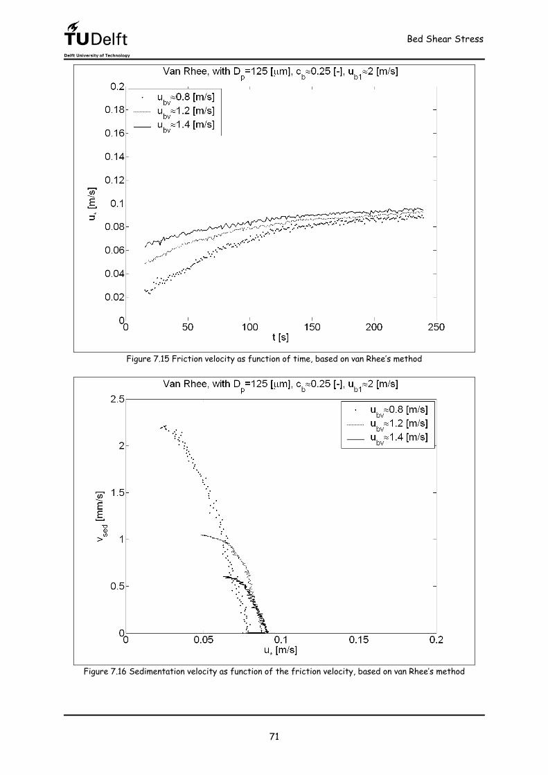
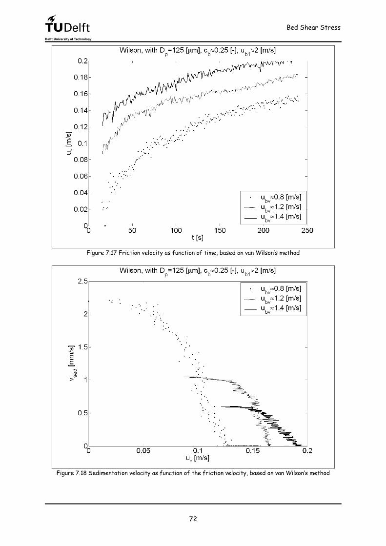
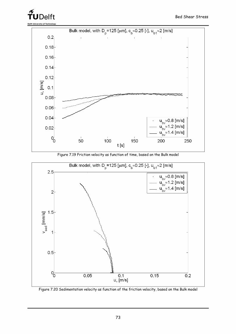
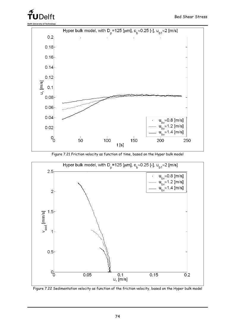
7.3 Modification of van Rhee’s model..................................................................................................60 7.4 Modification of Wilson’s model......................................................................................................60 7.5 Bulk model...........................................................................................................................................62 7.6 Hyper bulk model ..............................................................................................................................63 7.7 Results on calculating the friction velocity ................................................................................70
Contents
vi
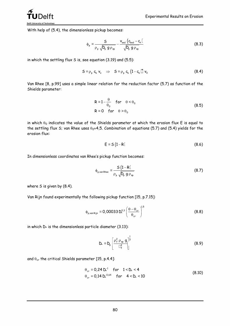
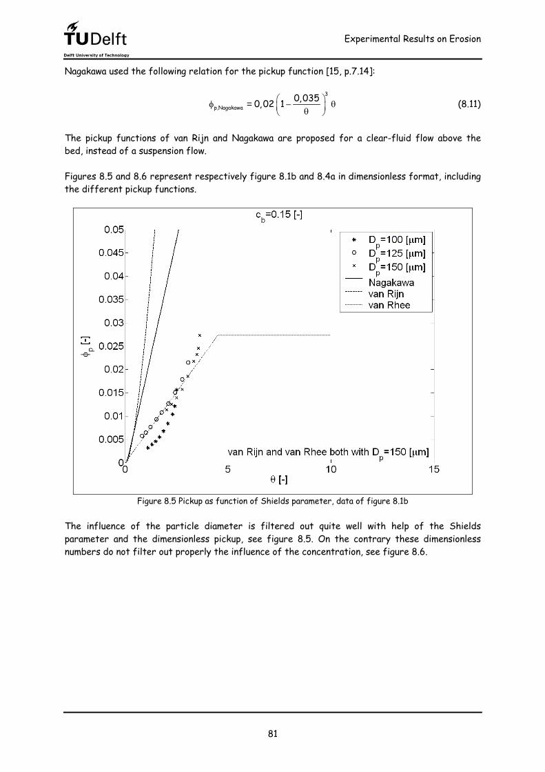
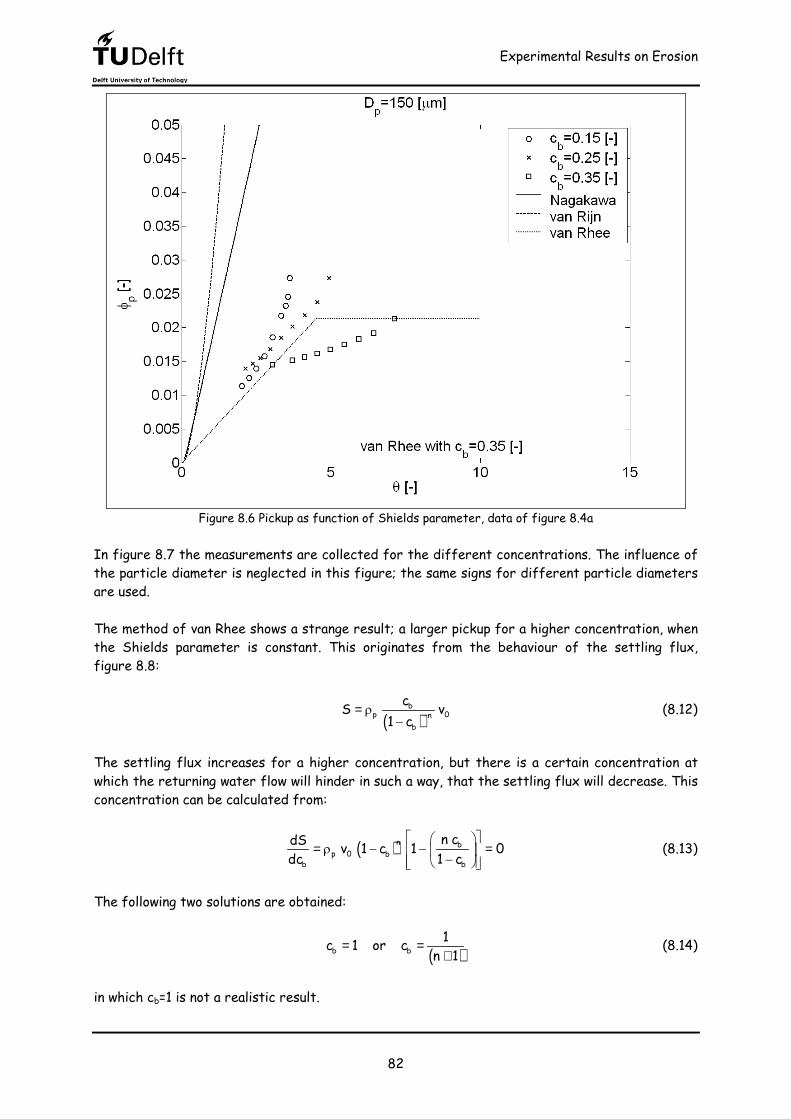
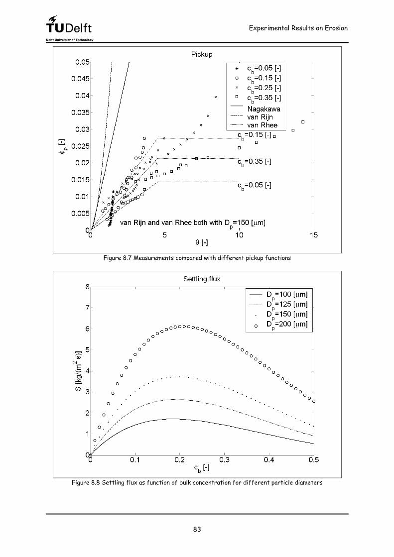
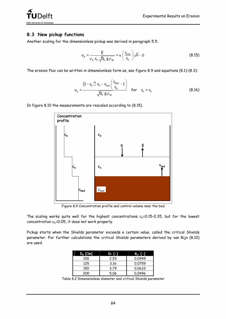
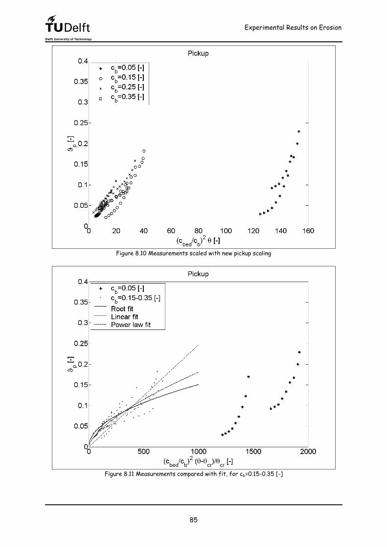
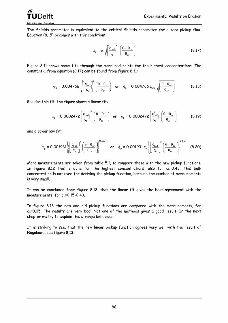
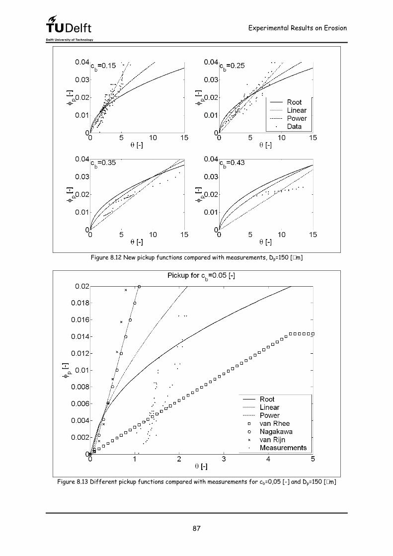
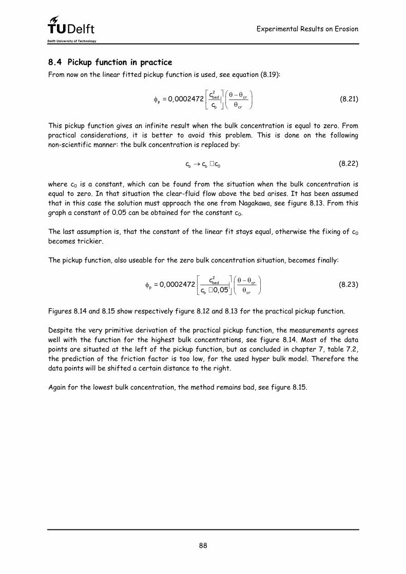
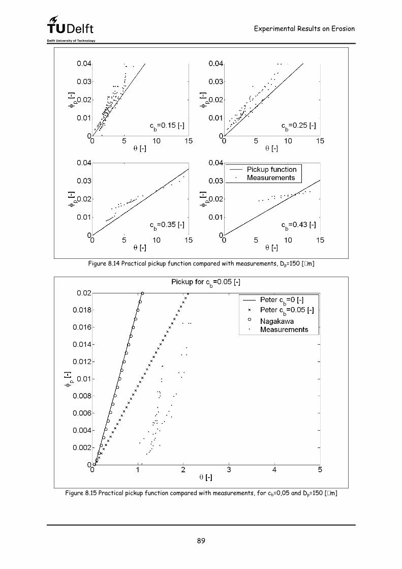
8 Experimental Results on Erosion ...........................................................................................................77 8.1 Sedimentation velocity versus friction velocity ........................................................................77 8.2 Existing pickup functions ................................................................................................................78 8.3 New pickup functions .......................................................................................................................84 8.4 Pickup function in practice..............................................................................................................88
9 The Road to Pickup ................................................................................................................................... 91 9.1 The measurements............................................................................................................................ 91 9.2 The friction velocity ........................................................................................................................ 91 9.3 The pickup function ..........................................................................................................................92 9.4 Discussion ...........................................................................................................................................93
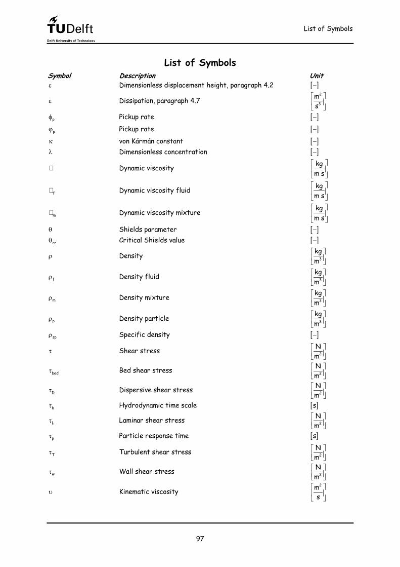
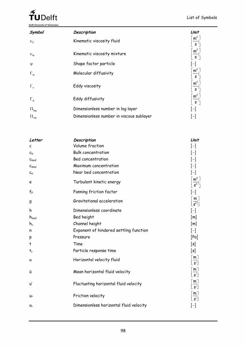
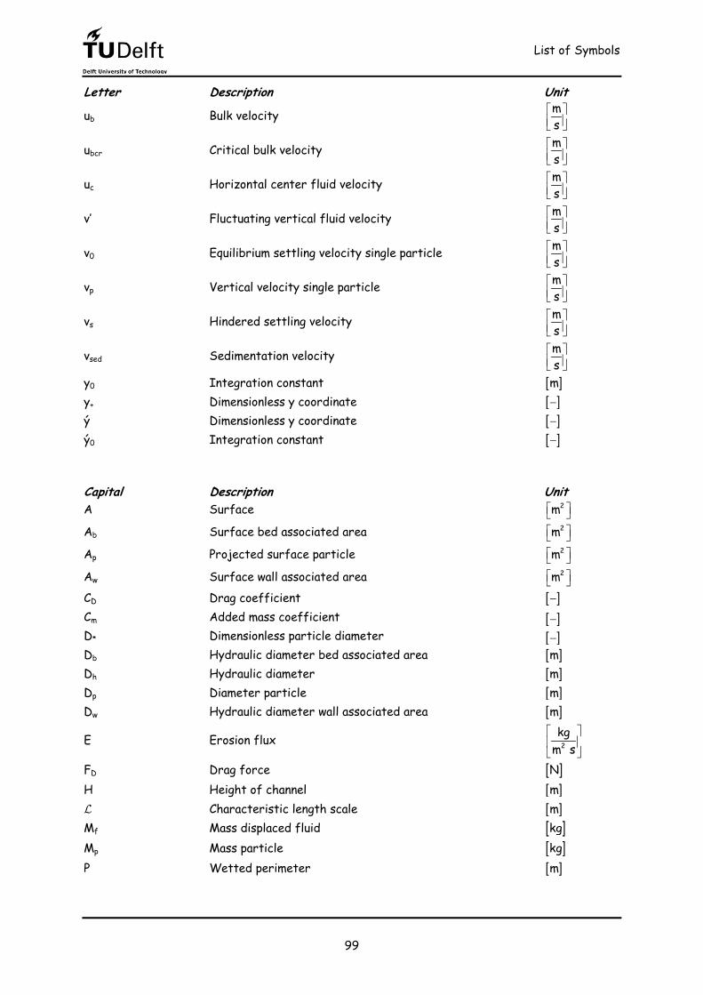
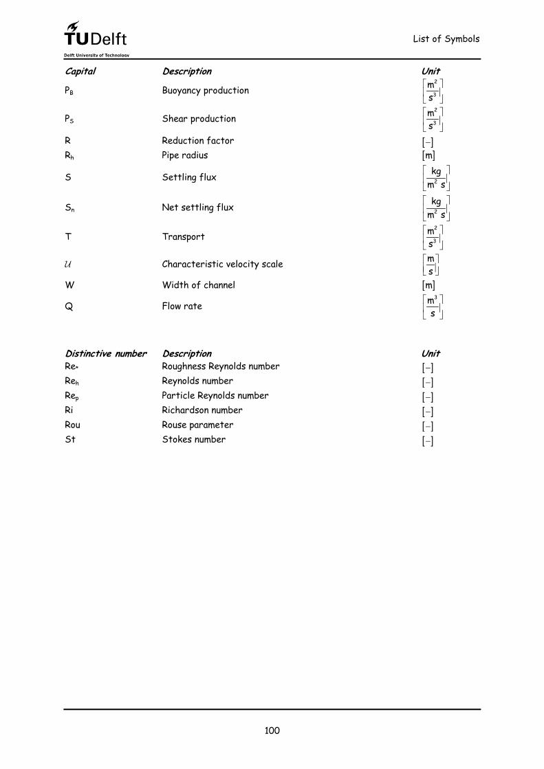
10 Conclusions and Recommendations ....................................................................................................95 List of Symbols .................................................................................................................................................97 References ....................................................................................................................................................... 101
Background and research aims
1
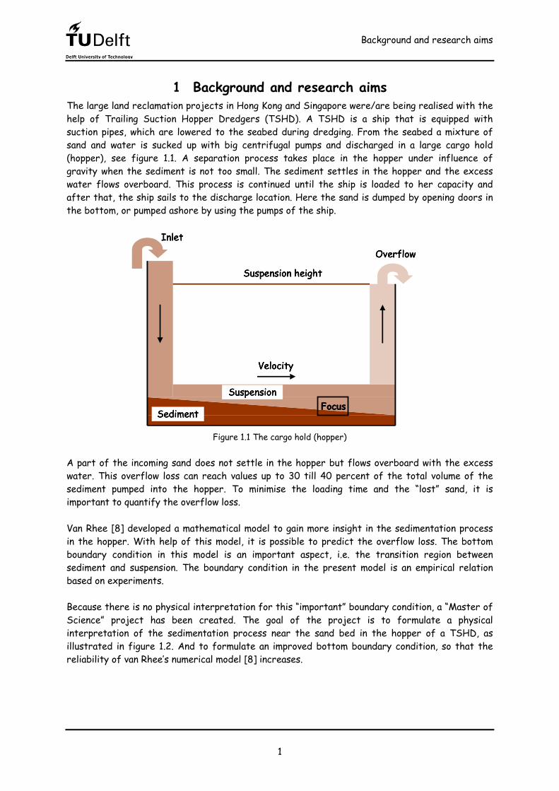
1 Background and research aims The large land reclamation projects in Hong Kong and Singapore were/are being realised with the help of Trailing Suction Hopper Dredgers (TSHD). A TSHD is a ship that is equipped with suction pipes, which are lowered to the seabed during dredging. From the seabed a mixture of sand and water is sucked up with big centrifugal pumps and discharged in a large cargo hold (hopper), see figure 1.1. A separation process takes place in the hopper under influence of gravity when the sediment is not too small. The sediment settles in the hopper and the excess water flows overboard. This process is continued until the ship is loaded to her capacity and after that, the ship sails to the discharge location. Here the sand is dumped by opening doors in the bottom, or pumped ashore by using the pumps of the ship.
Velocity
InletOverflow
SedimentSuspension
Suspension height
Focus
Velocity
InletOverflow
SedimentSuspension
Suspension height
Velocity
InletOverflow
SedimentSuspension
Suspension height
Focus Figure 1.1 The cargo hold (hopper)
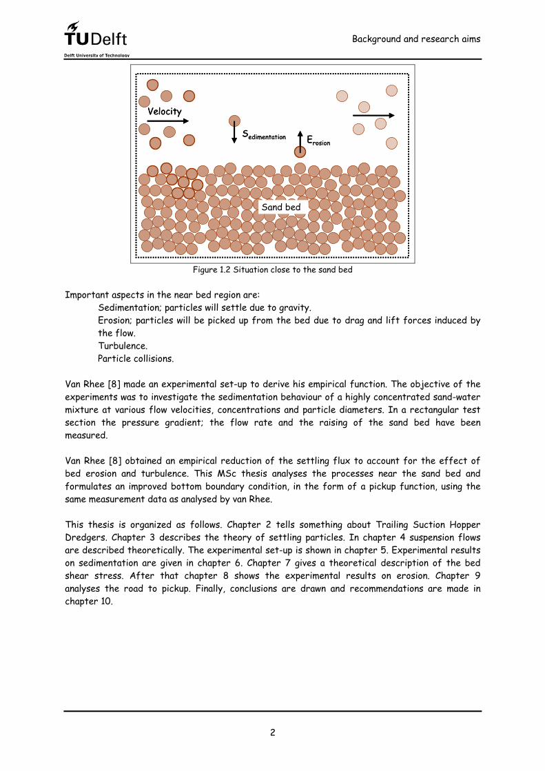
A part of the incoming sand does not settle in the hopper but flows overboard with the excess water. This overflow loss can reach values up to 30 till 40 percent of the total volume of the sediment pumped into the hopper. To minimise the loading time and the “lost” sand, it is important to quantify the overflow loss. Van Rhee [8] developed a mathematical model to gain more insight in the sedimentation process in the hopper. With help of this model, it is possible to predict the overflow loss. The bottom boundary condition in this model is an important aspect, i.e. the transition region between sediment and suspension. The boundary condition in the present model is an empirical relation based on experiments. Because there is no physical interpretation for this “important” boundary condition, a “Master of Science” project has been created. The goal of the project is to formulate a physical interpretation of the sedimentation process near the sand bed in the hopper of a TSHD, as illustrated in figure 1.2. And to formulate an improved bottom boundary condition, so that the reliability of van Rhee’s numerical model [8] increases.
Background and research aims
2
VelocitySedimentation
Sand bed
Erosion
VelocitySedimentation
Sand bed
Erosion
Figure 1.2 Situation close to the sand bed Important aspects in the near bed region are:
• Sedimentation; particles will settle due to gravity. • Erosion; particles will be picked up from the bed due to drag and lift forces induced by
the flow. • Turbulence. • Particle collisions.
Van Rhee [8] made an experimental set-up to derive his empirical function. The objective of the experiments was to investigate the sedimentation behaviour of a highly concentrated sand-water mixture at various flow velocities, concentrations and particle diameters. In a rectangular test section the pressure gradient; the flow rate and the raising of the sand bed have been measured. Van Rhee [8] obtained an empirical reduction of the settling flux to account for the effect of bed erosion and turbulence. This MSc thesis analyses the processes near the sand bed and formulates an improved bottom boundary condition, in the form of a pickup function, using the same measurement data as analysed by van Rhee. This thesis is organized as follows. Chapter 2 tells something about Trailing Suction Hopper Dredgers. Chapter 3 describes the theory of settling particles. In chapter 4 suspension flows are described theoretically. The experimental set-up is shown in chapter 5. Experimental results on sedimentation are given in chapter 6. Chapter 7 gives a theoretical description of the bed shear stress. After that chapter 8 shows the experimental results on erosion. Chapter 9 analyses the road to pickup. Finally, conclusions are drawn and recommendations are made in chapter 10.
Trailing Suction Hopper Dredger
3
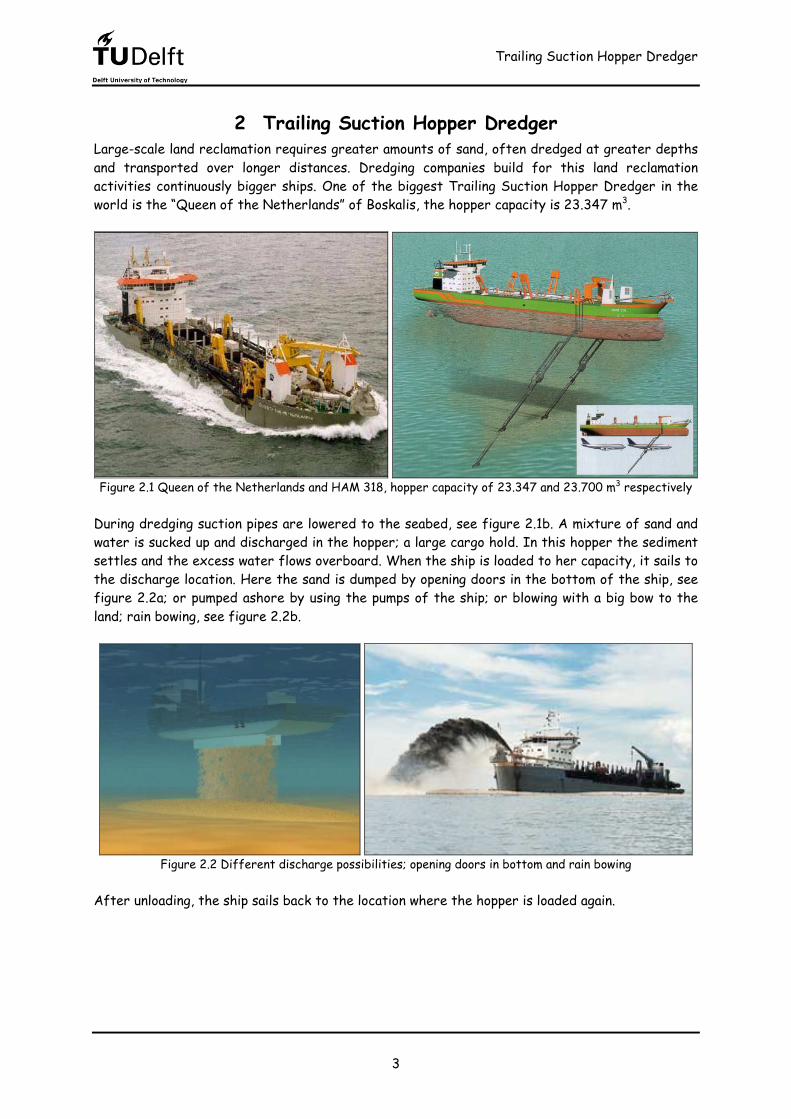
2 Trailing Suction Hopper Dredger Large-scale land reclamation requires greater amounts of sand, often dredged at greater depths and transported over longer distances. Dredging companies build for this land reclamation activities continuously bigger ships. One of the biggest Trailing Suction Hopper Dredger in the world is the “Queen of the Netherlands” of Boskalis, the hopper capacity is 23.347 m3.
Figure 2.1 Queen of the Netherlands and HAM 318, hopper capacity of 23.347 and 23.700 m3 respectively During dredging suction pipes are lowered to the seabed, see figure 2.1b. A mixture of sand and water is sucked up and discharged in the hopper; a large cargo hold. In this hopper the sediment settles and the excess water flows overboard. When the ship is loaded to her capacity, it sails to the discharge location. Here the sand is dumped by opening doors in the bottom of the ship, see figure 2.2a; or pumped ashore by using the pumps of the ship; or blowing with a big bow to the land; rain bowing, see figure 2.2b.
Figure 2.2 Different discharge possibilities; opening doors in bottom and rain bowing After unloading, the ship sails back to the location where the hopper is loaded again.
Trailing Suction Hopper Dredger
4
An example of a big land reclamation project is Palm Island in Dubai, see figure 2.3.
Figure 2.3 Palm Island, Dubai Palm Island is world’s largest man-made island. It has a diameter of 5 kilometer and a crescent breakwater of 11 kilometer. They used 60 million cubic meter sand to build this island in the shape of a huge palm tree. The Palm will host residential homes, 40 luxury hotels, entertainment and shopping facilities, theme parks and water sport and diving facilities. Often they call this island the 8th wonder of the world. Another mega land reclamation project is The World, also in Dubai, see figure 2.4.
Figure 2.4 The World, Dubai The World consists of 200 islands, together they form the shape of the world. It covers 5,6 million squared meter, of which 0,9 million squared meter is beach. The diameter of the island is approximately 5,5 kilometer. With this project they want to increase tourism in Dubai, with the current number of visitors standing at 5 million due to reach 10 million by 2007 and an incredible 40 million by 2015.
Settling of Particles in Stagnant Flow
5
3 Settling of Particles in Stagnant Flow This Chapter gives a theoretical background for single particle motion in paragraph 3.1-3.4 and multiple particle motion in paragraph 3.5.
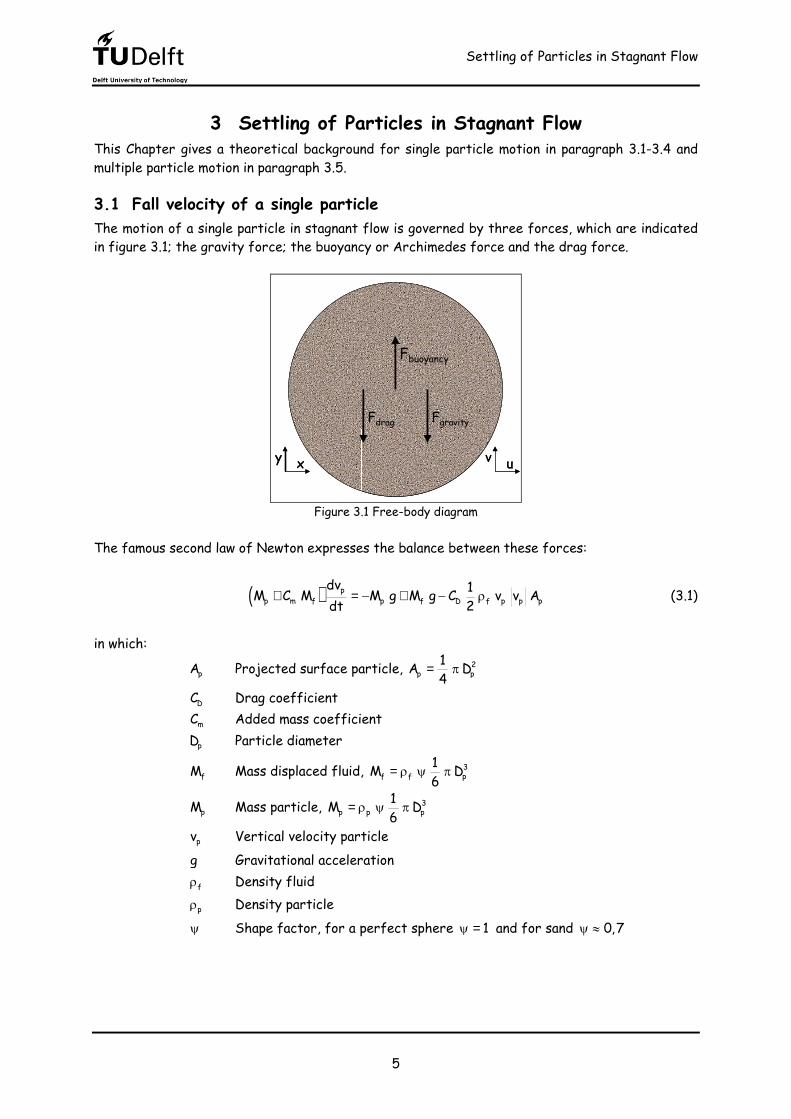
3.1 Fall velocity of a single particle The motion of a single particle in stagnant flow is governed by three forces, which are indicated in figure 3.1; the gravity force; the buoyancy or Archimedes force and the drag force.
Fgravity
xy uv
Fbuoyancy
Fdrag Fgravity
xy uv
Fbuoyancy
Fdrag
Figure 3.1 Free-body diagram The famous second law of Newton expresses the balance between these forces: ( )+ = − + − ρp
p m p p p pDf f fdv 1M C M M g M g C v v Adt 2 (3.1)
in which:
pA Projected surface particle, 2p p
1A D4= π DC Drag coefficient mC Added mass coefficient pD Particle diameter fM Mass displaced fluid, 3
pf f1M D6= ρ ψ π
pM Mass particle, 3p p p
1M D6= ρ ψ π pv Vertical velocity particle
g Gravitational acceleration fρ Density fluid pρ Density particle ψ Shape factor, for a perfect sphere 1ψ = and for sand 0,7ψ ≈
Settling of Particles in Stagnant Flow
6
Starting from rest the particle will accelerate until it reaches an equilibrium fall velocity v0. In that case (3.1) becomes: p sp
0D
4 D gv 3 Cψ ρ
= (3.2) where spρ is the specific density, defined by: p f
spf
ρ − ρρ = ρ (3.3)
3.2 Drag coefficient From a dimensional analysis, it follows that the drag coefficient CD in (3.1) depends on the particle Reynolds number Rep, defined by: p pf
pf
v D inertia forcesRe viscous forcesρ
= =µ
(3.4) For Stokes flow the drag coefficient for spheres can be calculated exact by the so-called law of Stokes, Bird et al. [25, p.186]: = ≤pD
p
24C for Re 1Re (3.5) For turbulent flow the drag coefficient for spheres becomes more or less constant. Lapple [1, p.287] used for example: = ≤ ≤ ⋅3 5
pDC 0,44 for 10 Re 2 10 (3.6) For the transition regime many empirical formulas are available. Khan and Richardson [2] used the following relation: ( )− −= + < < ⋅3,450,31 0,06 2 5
p p pDC 2,25 Re 0,36 Re for 10 Re 3 10 (3.7) For sand particles the behaviour of the drag coefficient is different. Julien [3, p.74] used: = + ≤ 4
pDp
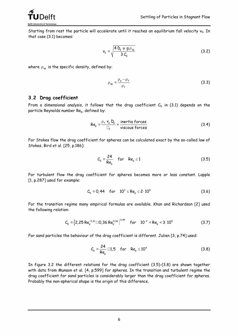
24C 1,5 for Re 10Re (3.8) In figure 3.2 the different relations for the drag coefficient (3.5)-(3.8) are shown together with data from Munson et al. [4, p.599] for spheres. In the transition and turbulent regime the drag coefficient for sand particles is considerably larger than the drag coefficient for spheres. Probably the non-spherical shape is the origin of this difference.
Settling of Particles in Stagnant Flow
7
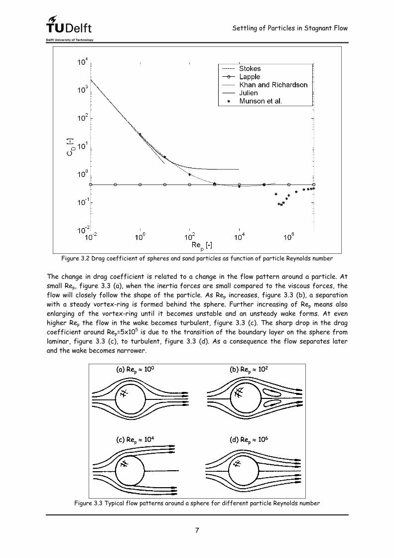
Figure 3.2 Drag coefficient of spheres and sand particles as function of particle Reynolds number The change in drag coefficient is related to a change in the flow pattern around a particle. At small Rep, figure 3.3 (a), when the inertia forces are small compared to the viscous forces, the flow will closely follow the shape of the particle. As Rep increases, figure 3.3 (b), a separation with a steady vortex-ring is formed behind the sphere. Further increasing of Rep means also enlarging of the vortex-ring until it becomes unstable and an unsteady wake forms. At even higher Rep the flow in the wake becomes turbulent, figure 3.3 (c). The sharp drop in the drag coefficient around Rep=5x10⁵ is due to the transition of the boundary layer on the sphere from laminar, figure 3.3 (c), to turbulent, figure 3.3 (d). As a consequence the flow separates later and the wake becomes narrower.
(a) Rep ≈ 100 (b) Rep ≈ 102
(c) Rep ≈ 104 (d) Rep ≈ 106
(a) Rep ≈ 100 (b) Rep ≈ 102
(c) Rep ≈ 104 (d) Rep ≈ 106
Figure 3.3 Typical flow patterns around a sphere for different particle Reynolds number
Settling of Particles in Stagnant Flow
8
3.3 Equilibrium fall velocity of a single particle Combining (3.2) and (3.5) yields the following expression for the equilibrium fall velocity of a spherical particle in the Stokes regime:
2p sp f
0 pf
D gv for Re 118ρ ρ
= ≤µ
(3.9) The equilibrium fall velocity for a non-spherical sand particle can be obtained from (3.2) and (3.8): p sp 4
0 p
p
4 D gv for Re 10243 1,5Re
ψ ρ= ≤
+
(3.10)
The results of equations (3.9) and (3.10) are equal when Rep<<1. Formula (3.10) is not in closed form while Rep is linear in v0. Therefore an iteration procedure is needed to calculate v0 exactly. However the literature provides many equations giving an approximate relation for v0 in closed form. For example Zhang [5] used:
2
f f0 sp p
p pf fv 13,95 1,09 g D 13,95D D
µ µ = + ρ − ρ ρ (3.11)
Julien [3, p.75] used: 1
3 4f 20 p*pf
8v 1 0,0139 D 1 for Re 10Dµ = + − ≤ ρ
(3.12) in which D* is the dimensionless particle diameter, defined by:
1
2 3spfp* 2
f
gD D ρ ρ=
µ (3.13)
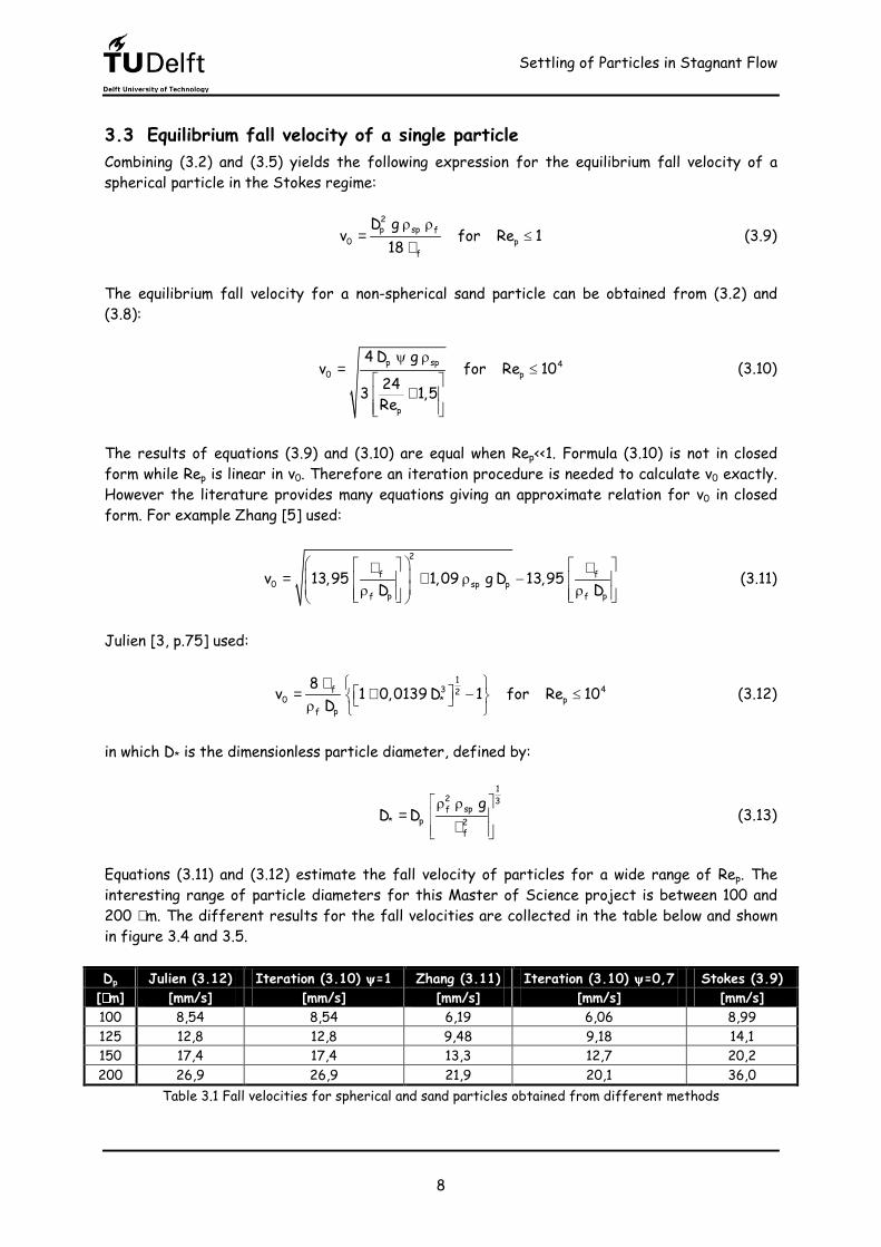
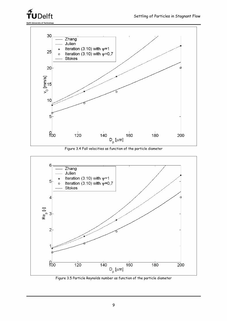
Equations (3.11) and (3.12) estimate the fall velocity of particles for a wide range of Rep. The interesting range of particle diameters for this Master of Science project is between 100 and 200 µm. The different results for the fall velocities are collected in the table below and shown in figure 3.4 and 3.5. Dp Julien (3.12) Iteration (3.10) ψψψψ=1 Zhang (3.11) Iteration (3.10) ψψψψ=0,7 Stokes (3.9)
Table 3.1 Fall velocities for spherical and sand particles obtained from different methods
Settling of Particles in Stagnant Flow
9
Figure 3.4 Fall velocities as function of the particle diameter
Figure 3.5 Particle Reynolds number as function of the particle diameter
Settling of Particles in Stagnant Flow
10
3.4 Particle response time The particle response time is defined as the time needed for a particle at rest to reach 99% of the equilibrium fall velocity. For calculating the particle response time equation (3.1) must be solved. This equation is rewritten according to: ( )
( ) ( )p fp 2f D
ppp m p mf f
gdv (t) 3 C (t) v (t)dt DC 4 Cρ − ρ ρ− = − +ρ + ρ ψ ρ + ρ (3.14)
For spherical particles in Stokes flow (3.5) reads equation (3.14): ( )
With help of the initial condition pv (0) 0= , the solution reads: ( )t
pv (t) 1 e−βα= −β (3.16) The particle response time tr follows from p r 0v (t ) 0,99 v= , with v0 given by (3.9): 2
r r p p1 99t ln 1 t D for Re 1100
= − − ⇒ ≤ β ∼ (3.17) The value of tr for non spherical sand particles is found from solving equation (3.14) with equation (3.8) for CD: ( )
( ) ( )p fp pf f
p2p pfp m p mf f
gdv (t) 1,5 v (t)3 24 v (t)dt D DC 4 Cρ − ρ ρ µ− = − + + ρρ + ρ ψ ρ + ρ
(3.18)
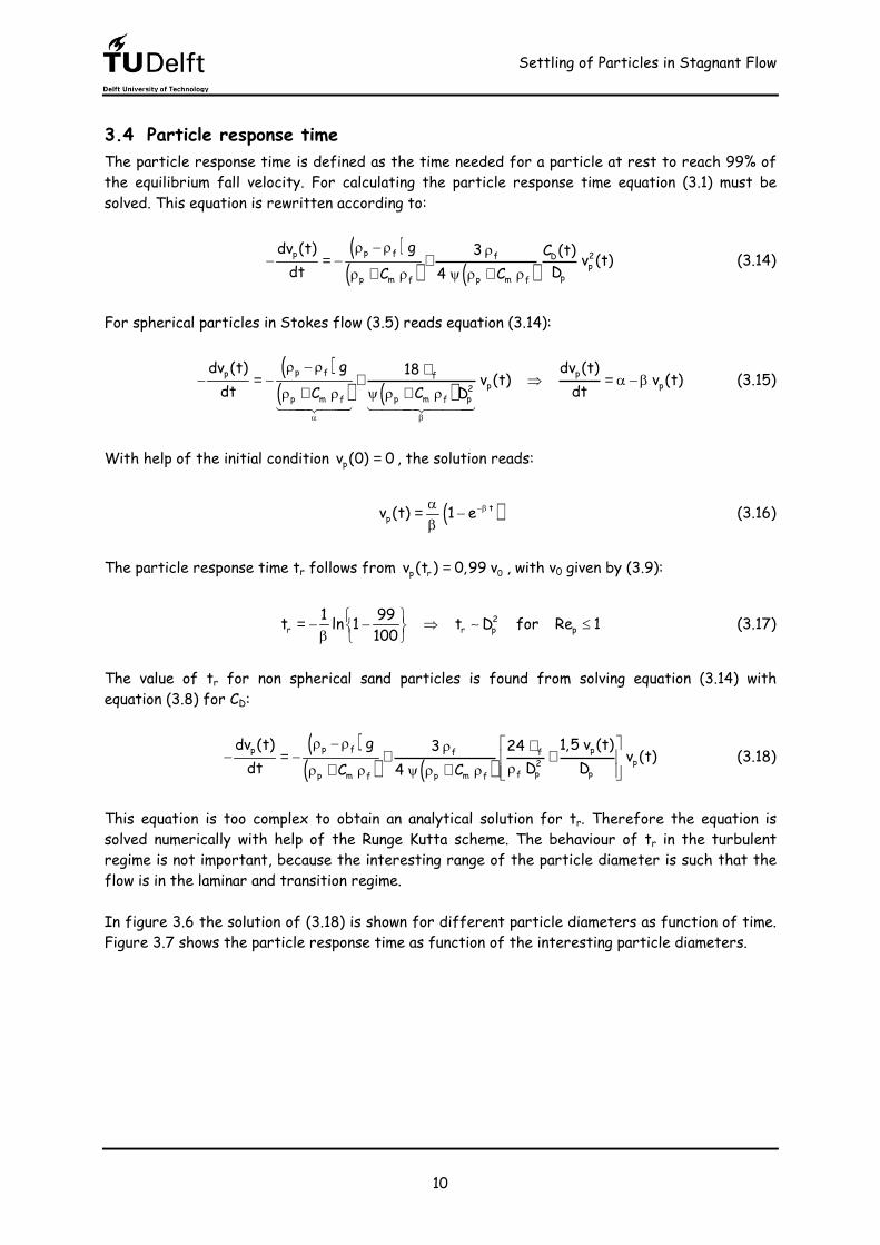
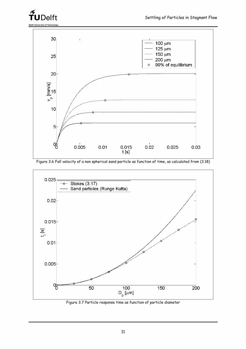
This equation is too complex to obtain an analytical solution for tr. Therefore the equation is solved numerically with help of the Runge Kutta scheme. The behaviour of tr in the turbulent regime is not important, because the interesting range of the particle diameter is such that the flow is in the laminar and transition regime. In figure 3.6 the solution of (3.18) is shown for different particle diameters as function of time. Figure 3.7 shows the particle response time as function of the interesting particle diameters.
Settling of Particles in Stagnant Flow
11
Figure 3.6 Fall velocity of a non spherical sand particle as function of time, as calculated from (3.18)
Figure 3.7 Particle response time as function of particle diameter
Settling of Particles in Stagnant Flow
12
3.5 Hindered settling Unless a suspension is very dilute, the settling velocity will be reduced. This is described in terms of a hindered settling function f(c). The hindered settling effect is caused by displaced fluid which creates a returning flow. Generally the influence of the volume fraction c is written as: s 0v f(c) v= (3.19) Hindered settling functions are typically determined empirically by measuring the fall velocity. Burgers [1, p.289] derived: 1f(c) 1 6,875 c=
+ (3.20)
This relation checks well for the range of c smaller then 0,05. Garside et al. [7, p.166] used the following semi-empirical formula: ( )
( )
2
5 c 1 c13 3
1 cf(c)1 c e
−−
= +
(3.21)
The relation of Richardson & Zaki is well-known for hindered settling: ( )nf(c) 1 c= − (3.22) The exponent n of the hindered settling function (3.22) is a function of the particle Reynolds number. For low or high particle Reynolds numbers the exponent is constant. The exponent varies in the transition regime. Richardson & Zaki [8, p.31] found: p
0,03p p
Re 0,2 n 4,650,2 Re 1 n 4,35 Re−
< ⇒ =
≤ < ⇒ =
0,1p p
p
1 Re 200 n 4,45 ReRe 200 n 2,39
−≤ < ⇒ =
> ⇒ = (3.23)
The equation of Rowe [8, p.31] can be used to achieve a smooth presentation:
0,75p p
0,75p p
a b Re 4,7 0,41 Ren n1 c Re 1 0,175 Reα
α+ +
= ⇒ =+ +
(3.24)
Dp [µµµµm] Rep [-] n [-] 100 0,854 4,38
125 1,60 4,23
150 2,61 4,08
200 5,38 3,80
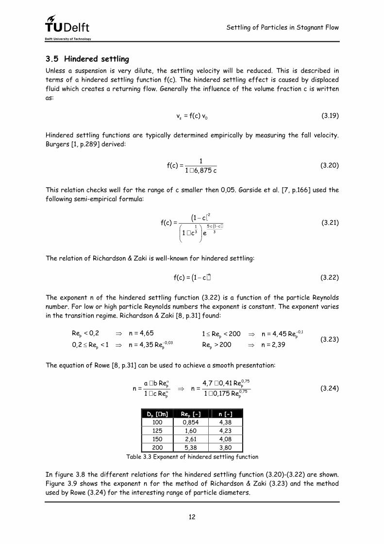
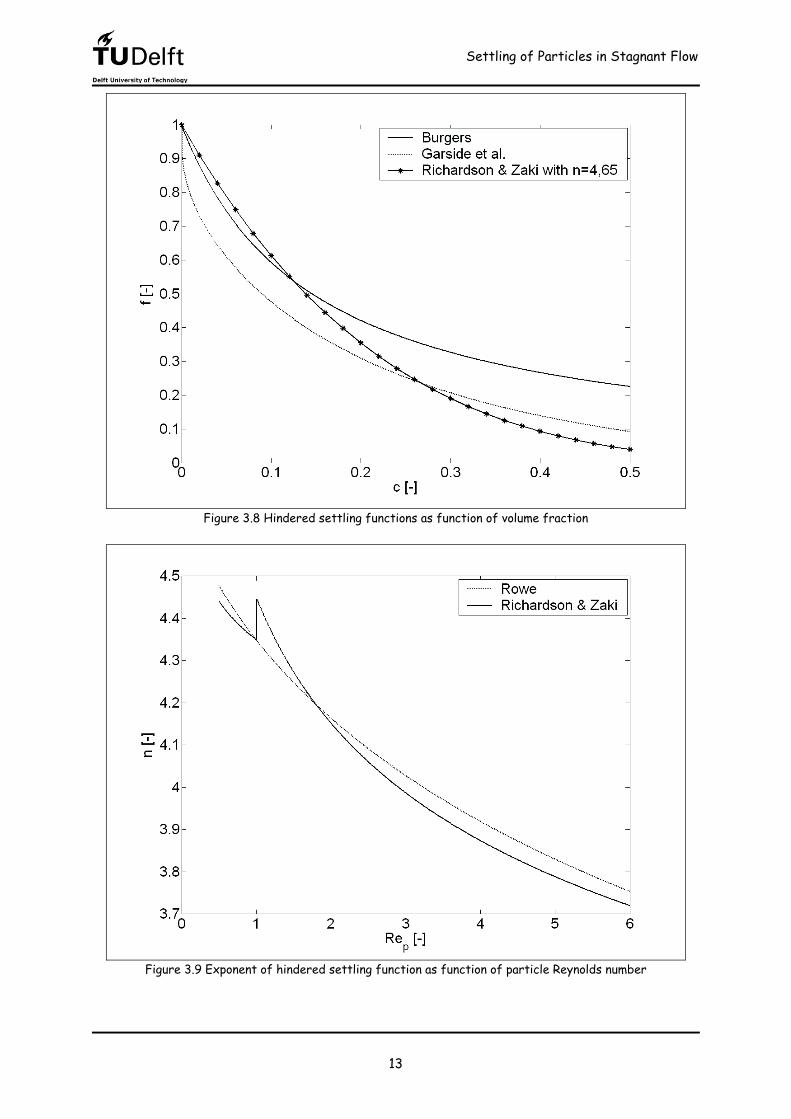
Table 3.3 Exponent of hindered settling function In figure 3.8 the different relations for the hindered settling function (3.20)-(3.22) are shown. Figure 3.9 shows the exponent n for the method of Richardson & Zaki (3.23) and the method used by Rowe (3.24) for the interesting range of particle diameters.
Settling of Particles in Stagnant Flow
13
Figure 3.8 Hindered settling functions as function of volume fraction
Figure 3.9 Exponent of hindered settling function as function of particle Reynolds number
Settling of Particles in Stagnant Flow
14
The large volume of experimental data collected on hindered settling shows considerable scatter and do not uniquely define a universal hindered settling function. Two possible reasons for the difficulty in uniquely determining the hindered settling functions are [7, p.169-174]:
• Inaccuracies in the Stokes velocity: The hindered settling function is based on the difference between the measured sedimentation velocity of a suspension and the Stokes fall velocity of a particle. It is difficult to calculate the Stokes velocity exactly because it is difficult to measure the particle radius more accurately than to within several percent (diameter is squared in Stokes settling, see equation (3.9)).
• Interfacial spreading: Most determinations of hindered settling functions are based on visual measurements of the fall velocity of the interface separating the suspension regime from the clarified fluid above. An uncertainty with this procedure arises because the interface is diffuse.
Flow of Suspensions
15
4 Flow of Suspensions This chapter gives some typical properties of suspensions/mixtures most compared with standard (Newtonian) properties. Paragraph 4.1-4.2 describes typical Newtonian velocity profiles. In paragraph 4.3 eddy viscosity profiles are described. The influence of particle collisions is added in paragraphs 4.4 and 4.5. The last two paragraphs try to estimate the influence of buoyancy.
4.1 Newtonian velocity profile in turbulent flow conditions Turbulent flows are characterized by irregular velocity fluctuations. Reynolds splits every property into a mean and a fluctuating part, for example the velocity: u u u'= + (4.1) Substituting into the Navier Stokes equation and taking the time mean gives for the momentum equation in the mainstream direction, Streeter et al. [9, p.275]: 2pDu u u uu' u' v' u'w'Dt x x x y y z z
The three correlation terms 2u'−ρ , u' v'−ρ and u'w'−ρ are called turbulent stresses. In duct and boundary layer flow the stress u' v'−ρ is dominant. When the turbulence is also stationary and horizontal homogeneous, the momentum equation will reduce to the following simplified form, Nieuwstadt [11, p.63]:
�∂ ∂τ ∂= − + τ = τ + τ = µ − ρ∂ ∂ ∂ ���L T
turbulentviscous
p u0 with u' v'x y y (4.3)
in which τ is the shear stress existing of a laminar τL and a turbulent part τT. From now on the over bar for the mean velocity and the mean pressure is omitted in order to simplify the notation. The Boussinesq hypothesis is used [11, p.58] to handle the correlation term in (4.3): v
uu' v' y∂− = Γ ∂ (4.4)
where Γv is the eddy viscosity. Using the Prandtl mixing length hypothesis [11, p.61] gives for the eddy viscosity: 2
vu uy y∂ ∂⇒ Γ = =∂ ∂∼U L U L L (4.5)
in which L is the Prandtl mixing length and U is a characteristic velocity scale for the large scale eddies. The corresponding turbulent shear stress (4.3) can be written as: ∂ ∂τ = −ρ = ρ = ρ Γ ∂ ∂
22
vTu uu' v' y yL (4.6)
Flow of Suspensions
16
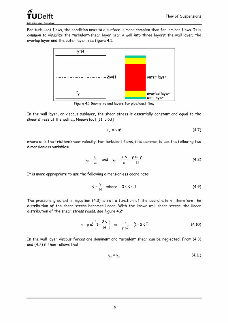
For turbulent flows, the condition next to a surface is more complex than for laminar flows. It is common to visualize the turbulent-shear layer near a wall into three layers; the wall layer; the overlap layer and the outer layer, see figure 4.1.
y=H
y
2y=H
wall layeroverlap layer
outer layer
y=H
y
2y=H
wall layeroverlap layer
outer layer
Figure 4.1 Geometry and layers for pipe/duct flow In the wall layer, or viscous sublayer, the shear stress is essentially constant and equal to the shear stress at the wall τw, Nieuwstadt [11, p.63]: 2
w *uτ = ρ (4.7) where u* is the friction/shear velocity. For turbulent flows, it is common to use the following two dimensionless variables: * *
*
u y u yuu and yu+ +
ρ= = =υ µ
(4.8) It is more appropriate to use the following dimensionless coordinate: yý where 0 ý 1H= ≤ ≤ (4.9) The pressure gradient in equation (4.3) is not a function of the coordinate y, therefore the distribution of the shear stress becomes linear. With the known wall shear stress, the linear distribution of the shear stress reads, see figure 4.2: ( )τ τ = ρ − ⇒ = − ρ
2* 2
*
2 yu 1 1 2 ýH u (4.10) In the wall layer viscous forces are dominant and turbulent shear can be neglected. From (4.3) and (4.7) it then follows that: + +=u y (4.11)
Flow of Suspensions
17
In the overlap layer, or logarithmic layer, it is assumed that the shear stress is approximately equal to the shear stress at the wall. The turbulent shear stress dominates and the viscous shear stress in (4.3) is unimportant. The following equation must be solved for this layer: ∂ρ = ρ ∂
22 2*
uu yL (4.12) The only unknown parameter is the Prandtl mixing length L. Often it is assumed that this length is proportional to the distance y from the wall: = κ κ �y with 0,4L (4.13) in which κ is the Von Kármán constant. Equation (4.12) can now easily be solved: ( )+ = +κ 1
1u ln y C (4.14) in which C1 is an integration constant evaluated at a distance y0 from the wall, where the velocity hypothetically equals zero. Thus: +
= κ 0
y1u ln y (4.15) It follows from measurements that the integration constant is approximately equal to, Nieuwstadt [11, p.65]: υ=0
*y 0,135 u (4.16)
The viscous and logarithmic profile are connected at y+=11. The logarithmic velocity profile yields finally: ( )1u ln y 2,0+ + = + κ (4.17) In the outer layer, or mean region, the turbulent part of the shear stress dominates and the shear distribution is given by equation (4.10). The velocity in this region becomes, Nieuwstadt [11, p.64]: +
= − − + = β
32
22 yHu 1 C with H3 H LL (4.18)
in which C2 and β are unknown constants.
Flow of Suspensions
18
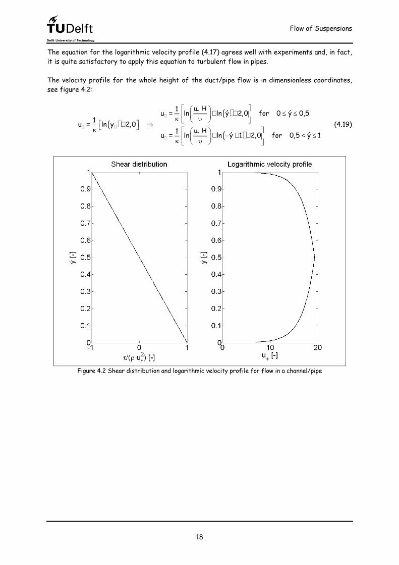
The equation for the logarithmic velocity profile (4.17) agrees well with experiments and, in fact, it is quite satisfactory to apply this equation to turbulent flow in pipes. The velocity profile for the whole height of the duct/pipe flow is in dimensionless coordinates, see figure 4.2:
( )( )
( )
*
*
u H1u ln ln ý 2,0 for 0 ý 0,51u ln y 2,0 u H1u ln ln ý 1 2,0 for 0,5 ý 1
+
+ +
+
= + + ≤ ≤ κ υ = + ⇒ κ = + − + + < ≤ κ υ
(4.19)
Figure 4.2 Shear distribution and logarithmic velocity profile for flow in a channel/pipe
Flow of Suspensions
19
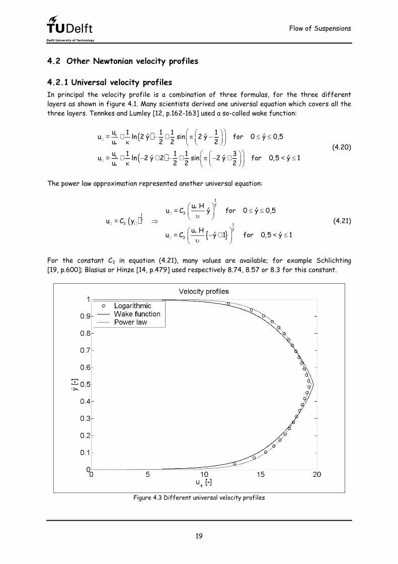
4.2 Other Newtonian velocity profiles 4.2.1 Universal velocity profiles In principal the velocity profile is a combination of three formulas, for the three different layers as shown in figure 4.1. Many scientists derived one universal equation which covers all the three layers. Tennkes and Lumley [12, p.162-163] used a so-called wake function:
( )
( )
+
+
= + − + π − ≤ ≤ κ = + − + − + π − + < ≤ κ
c*
c*
u 1 1 1 1u ln 2 ý sin 2 ý for 0 ý 0,5u 2 2 2u 1 1 1 3u ln 2 ý 2 sin 2 ý for 0,5 ý 1u 2 2 2
(4.20)
The power law approximation represented another universal equation:
( ){ }
17*
3173 1
7*3
u Hu C ý for 0 ý 0,5u C y
u Hu C ý 1 for 0,5 ý 1
+
+ +
+
= ≤ ≤ υ = ⇒ = − + < ≤ υ
(4.21)
For the constant C3 in equation (4.21), many values are available; for example Schlichting [19, p.600]; Blasius or Hinze [14, p.479] used respectively 8.74, 8.57 or 8.3 for this constant.
Figure 4.3 Different universal velocity profiles
Flow of Suspensions
20
4.2.2 Rough wall velocity profile Nikuradse investigated the effect of wall roughness on the velocity distribution for turbulent pipe flow. He measured velocity profiles at different Reynolds numbers, pipe diameters and grain sizes. The roughness elements generate eddies which affect the turbulence and hence the velocity close to the wall. The type of flow regime can be related to the ratio of the particle diameter Dp and the length scale of the viscous sublayer: = υ
p**
u DRe (4.22) in which Re* is the roughness Reynolds number. Based on experimental results, it was found that for hydraulically smooth walls follows, Julien [3, p.98]: υ= ⇒ = ≤υ
0 *0 *
*
y u 1y for Re 59 u 9 (4.23) and for hydraulically rough walls, Julien [3, p.95]: = ⇒ = ≥υ
p 0 * *0 *
D y u Rey for Re 7030 30 (4.24) and at least for the transition regime, van Rijn [15, p.2.4]: υ= + ⇒ = + < <υ
p 0 * *0 *
*
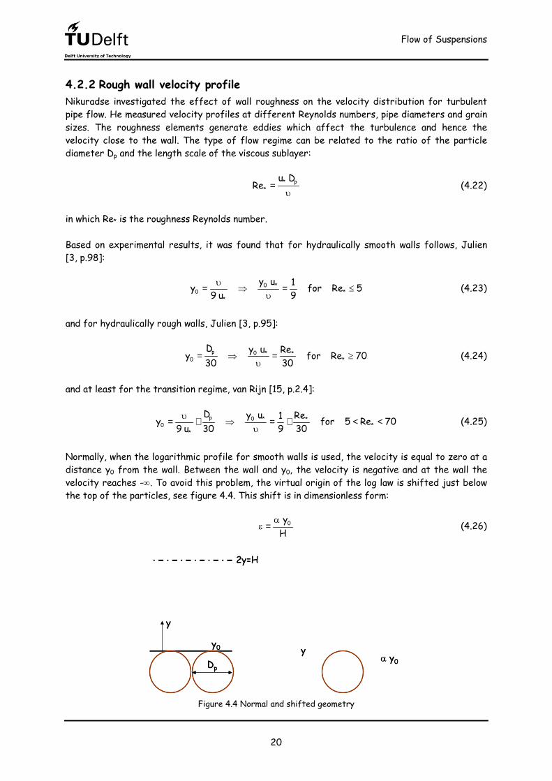
D y u Re1y for 5 Re 709 u 30 9 30 (4.25) Normally, when the logarithmic profile for smooth walls is used, the velocity is equal to zero at a distance y0 from the wall. Between the wall and y0, the velocity is negative and at the wall the velocity reaches -∞. To avoid this problem, the virtual origin of the log law is shifted just below the top of the particles, see figure 4.4. This shift is in dimensionless form: 0y
Hαε = (4.26)
yy0 y α y0
2y=H
Dp
yy0 y α y0
2y=H
Dp
Figure 4.4 Normal and shifted geometry
Flow of Suspensions
21
The velocity profile including the shift is described by:
( )
( )
00
0 0
y1u ln ý ln for 0 ý 0,5Hy y1u ln y y1u ln ý 1 2 ln for 0,5 ý 1H
+
+
+
= + ε − ≤ ≤ κ + α = ⇒ κ = − + + ε − < ≤ κ
(4.27)
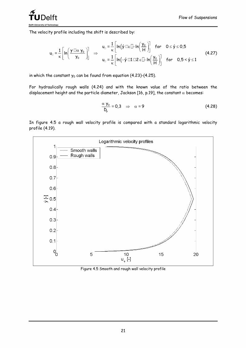
in which the constant y0 can be found from equation (4.23)-(4.25). For hydraulically rough walls (4.24) and with the known value of the ratio between the displacement height and the particle diameter, Jackson [16, p.19], the constant α becomes: α
= ⇒ α =0p
y 0,3 9D (4.28) In figure 4.5 a rough wall velocity profile is compared with a standard logarithmic velocity profile (4.19).
Figure 4.5 Smooth and rough wall velocity profile
Flow of Suspensions
22
4.3 Newtonian eddy viscosity profiles With the known velocity profile, it is possible to calculate the eddy viscosity as function of the height, with help of (4.6), the shear distribution of equation (4.10) and the logarithmic velocity profile of equation (4.19):
( )
( )( )
v*v*
ý 1 2 ý for 0 ý 0,5u Hý 1 1 2 ý for 0,5 ý 1u H
Γ= − ≤ ≤κ
Γ = − − + − < ≤κ (4.29)
This profile gives a value of zero at the center of the channel, while it follows from measurements that this value is not equal to zero. Schlichting [13, p.544] constructed from measurements the following distribution for the eddy viscosity: ( ) ( )2 2v
*
1 1 1 2 ý 1 2 1 2 ýu H 12Γ = − − + − κ (4.30)
Sometimes the profile is approximated by a simple parabolic distribution, Schlichting [13, p.538]: ( )v
*ý 1 ýu H
Γ= −κ (4.31)
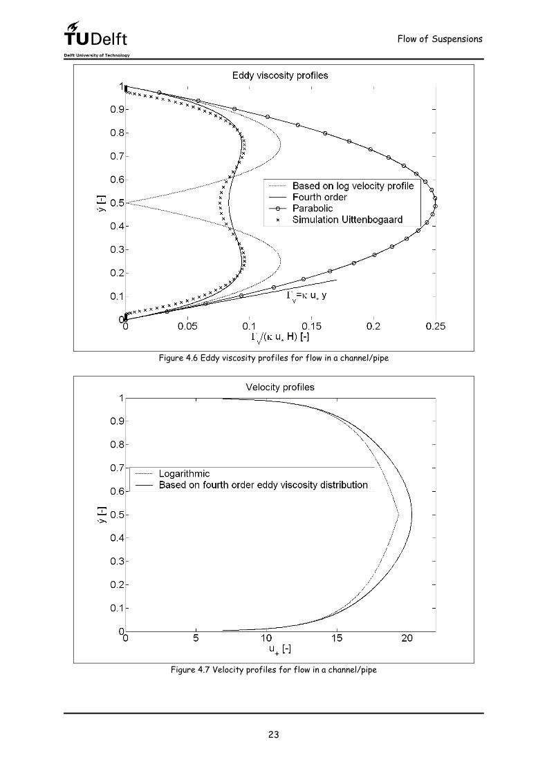
These solutions are not correct in the viscous sublayer, on account of absence of turbulent friction. In the logarithmic layer, the dimensionless eddy viscosity becomes equal to the dimensionless coordinate ý with help of a constant shear stress (4.7). In figure 4.6 the different relations for the eddy viscosity (4.29)-(4.31) are shown, together with simulation data from Uittenbogaard [personal communication]. Close to the wall all the relations give more or less the same result, but in the center of the channel they are completely different. It seems that in this region the Prandtl mixing length hypothesis (4.5) is wrong, while it predicts a characteristic velocity scale equal to zero, which is not correct. With help of the 4th order eddy viscosity profile (4.30), the linear distribution of the shear stress (4.10) and equation (4.6), it is possible to calculate the velocity distribution, see also figure 4.7: ( )
20
ý ý 11 1u ln 8 ý 8 ý 3 ý+
− = κ − + (4.32)
in which ý0 is an integration constant. This constant can be found, following the same procedure as used for the derivation of equation (4.16); connection with the viscous sublayer at y+=11:
2
* *0 2
* *
0.135 11 u H u Hý968 88 3u H u H
υ υ − = υ υ− +
(4.33)
Flow of Suspensions
23
Figure 4.6 Eddy viscosity profiles for flow in a channel/pipe
Figure 4.7 Velocity profiles for flow in a channel/pipe
Flow of Suspensions
24
With the known eddy viscosity, based on a logarithmic velocity distribution, and again with help of equation (4.6), it is possible to derive the Prandtl mixing length:
( )
( ) ( )
ý 1 2 ý for 0 ý 0,5Hý 1 1 2 ý for 0,5 ý 1H
= − ≤ ≤κ= − + − − < ≤κ
L
L (4.34)
The Prandtl mixing length, based on a 4th order eddy viscosity distribution, is represented by: ( ) ( ) ( )
2 21 11 1 2 ý 1 2 1 2 ýH 12 1 2 ý = − − + − κ −
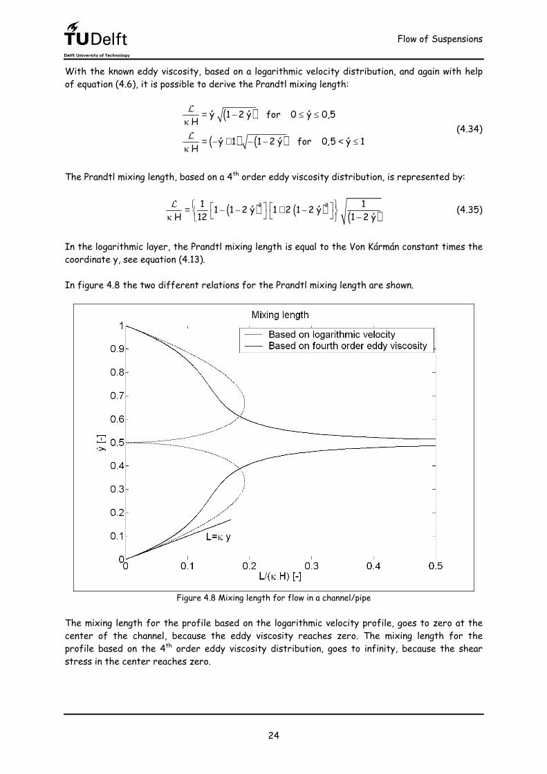
L (4.35) In the logarithmic layer, the Prandtl mixing length is equal to the Von Kármán constant times the coordinate y, see equation (4.13). In figure 4.8 the two different relations for the Prandtl mixing length are shown.
Figure 4.8 Mixing length for flow in a channel/pipe
The mixing length for the profile based on the logarithmic velocity profile, goes to zero at the center of the channel, because the eddy viscosity reaches zero. The mixing length for the profile based on the 4th order eddy viscosity distribution, goes to infinity, because the shear stress in the center reaches zero.
Flow of Suspensions
25
4.4 Density and viscosity of mixtures The density of a mixture ρm is the total mass of solids and water in the voids per unit of total volume. This can be defined, as a function of the volume fraction c, by: ( )m pf 1 c cρ = ρ − + ρ (4.36) and with the definition of the specific density ρsp (3.3): m
spf
1 cρ= + ρρ (4.37)
This is an easy linear relation for the density. However the dynamic viscosity of a mixture µm is not a simple linear relation for the whole interesting range of the volume fraction c. Einstein [10, p.253] derived for very dilute suspensions a linear relation for the viscosity: m
f1 2,5 c for c 0,05µ
= + ≤µ
(4.38) but for high concentrations, the viscosity deviates from the linear relation. For example Julien [3, p.190] added an extra term: ( )10 c 0,05m
f1 2,5 c e for c 0,05−µ
= + + >µ
(4.39) Bagnold [8, p.137-138] used the following relation for the dynamic viscosity of a mixture:
( )11
3m maxf
c1 1 with 12 c− µ λ = + λ + λ = − µ
(4.40)
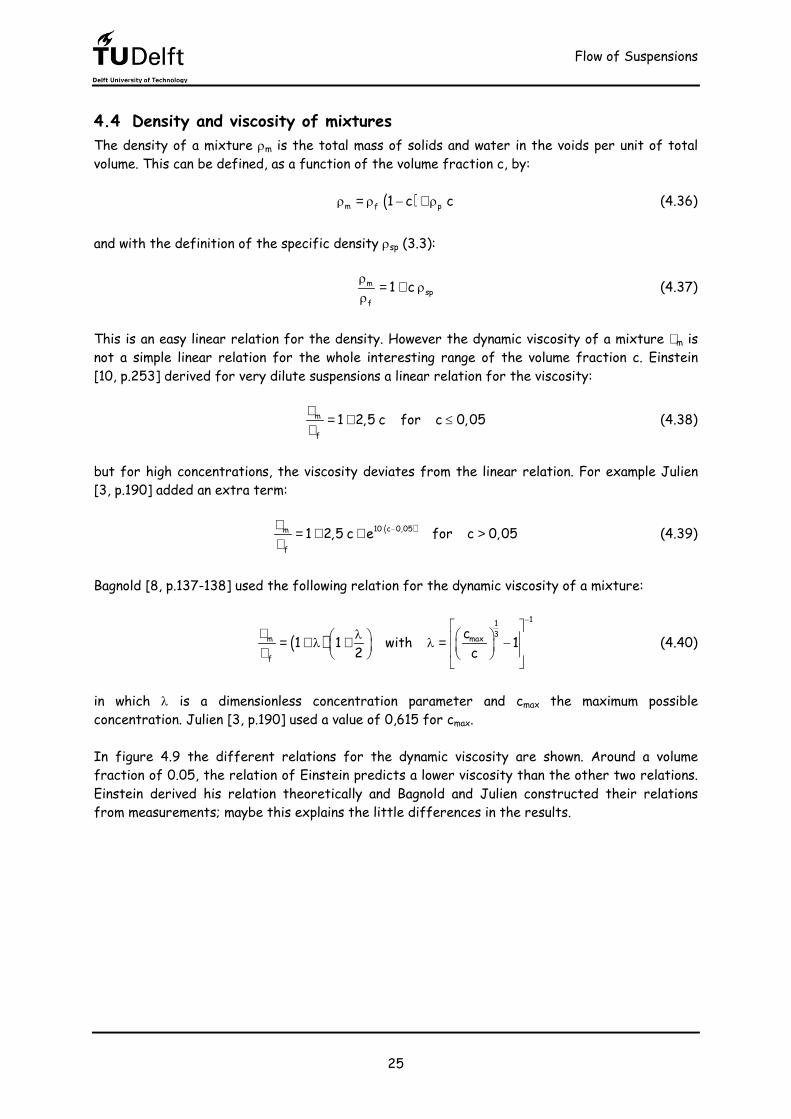
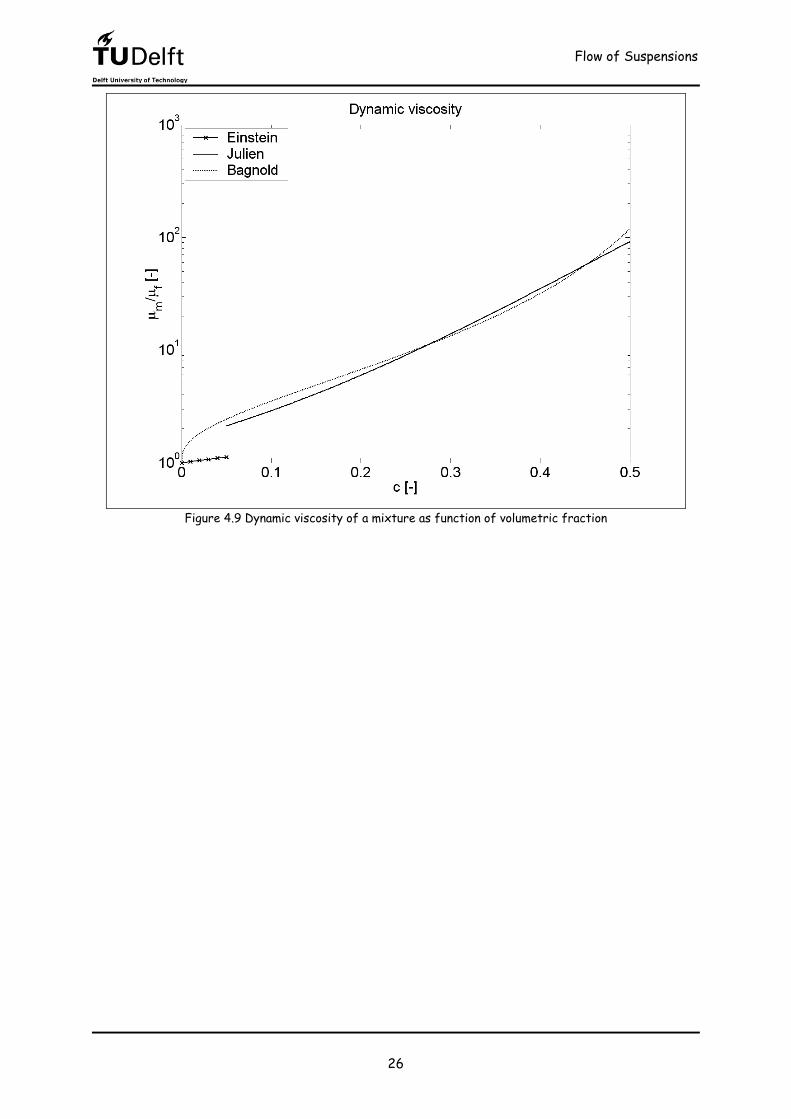
in which λ is a dimensionless concentration parameter and cmax the maximum possible concentration. Julien [3, p.190] used a value of 0,615 for cmax. In figure 4.9 the different relations for the dynamic viscosity are shown. Around a volume fraction of 0.05, the relation of Einstein predicts a lower viscosity than the other two relations. Einstein derived his relation theoretically and Bagnold and Julien constructed their relations from measurements; maybe this explains the little differences in the results.
Flow of Suspensions
26
Figure 4.9 Dynamic viscosity of a mixture as function of volumetric fraction
Flow of Suspensions
27
4.5 Extended non-Newtonian velocity profile In clear-water flows, the shear stress increases linearly with the rate of deformation in the laminar flow regime and the fluid is said to be Newtonian, see equation (4.3). Under large shear stresses, the boundary-layer flow becomes turbulent (except in the laminar sublayer) and the turbulent shear stress increases with the second power of the rate of deformation. The analysis of coarse sediment mixtures is somewhat more complex and involves an additional shear stress due to particle impact. Bagnold [3, p.189] defined the dispersive shear stress τD induced by the collision between sediment particles as:
− τ = ρ −
21 23 2max
p pD BDc duC 1 Dc dy (4.41)
in which: CBD Empirical parameter, ≅BDC 0,01
pρ Density particle cmax Maximum possible concentration, ≅maxc 0,615 c Volume fraction
pD Particle diameter dudy Velocity gradient
Combination of the dispersive shear stress (4.41) and (4.3) gives the following quadratic rheological model for course sediment mixtures:
− τ = τ + τ + τ = µ + ρ + ρ −
212 232 2max
L m m p pT D BDcdu du duC 1 Ddy dy c dyL (4.42)
4.5.1 Viscous sublayer The turbulent part of the shear stress can be neglected in the viscous sublayer, because laminar friction in this part of the flow dominates. The shear stress in the viscous sublayer is then:
− τ = µ + χ χ = ρ −
2123 2max
m p pBDcdu du with C 1 Ddy dy c (4.43)
The shear stress in this region is by definition equal to the density of the mixture times the friction velocity squared (4.7). The following formula arises: ρµ
+ − = χ χ
2 2m *m udu du 0dy dy (4.44)
Flow of Suspensions
28
With help of the abc-formula and assuming that the velocity gradient in the lower half of the channel is positive, the gradient becomes: ρµ µ
= − + + χ χ χ 2 2
m *m m udu 1dy 2 4 (4.45)
An important dimensionless number in the viscous sublayer is:
2
m *vis vis vis2
m m
dudycollision forces u and 0...10viscous forces
χ ρ χ Π = = ⇒ Π = Π ≈µ µ
(4.46) This dimensionless number expresses the ratio between the dispersive shear stress induced by collisions and the viscous shear stress. The velocity profile in dimensionless parameters reads, using the velocity gradient of (4.45): + +
= − + + Π Π visvis
1u 1 1 4 y2 (4.47) An interesting limit is the case that Πvis reaches zero. In that situation the Newtonian case is recovered. To calculate this limit the rule of l’Hospital is used, Stewart [18, p.306]:
→ → →
= ⇒ = y 0 y 0 y 0
dadya 0 alimit limit limit dbb 0 bdy
(4.48)
Applying the rule of l’Hospital gives the expected Newtonian result, see also equation (4.11):
visvis0 vis
1limit 1 1 4 1 u y2 + +Π → − + + Π = ⇒ = Π
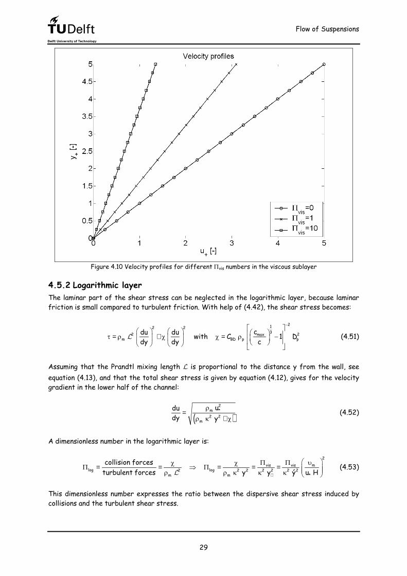
(4.49) In figure 4.10 the velocity profiles are shown for three different values of Πvis. The shear stress of (4.43) can be written in dimensionless form: 2L D
In table 4.1 the values are shown for the laminar and dispersive part of the shear stress for the three different values of Πvis, as used in figure 4.10. Increasing Πvis induces increasing behaviour of the dispersive part of the shear stress.
ΠΠΠΠvis ττττL/(ρρρρm u*2) ττττB/(ρρρρm u*2) 0 1 0
1 0,618 0,382 10 0,270 0,730
Table 4.1 Laminar and dispersive part of shear stress for different Πvis
Flow of Suspensions
29
Figure 4.10 Velocity profiles for different Πvis numbers in the viscous sublayer
4.5.2 Logarithmic layer The laminar part of the shear stress can be neglected in the logarithmic layer, because laminar friction is small compared to turbulent friction. With help of (4.42), the shear stress becomes:
− τ = ρ + χ χ = ρ −
212 232 2max
m p pBDcdu du with C 1 Ddy dy cL (4.51)
Assuming that the Prandtl mixing length L is proportional to the distance y from the wall, see equation (4.13), and that the total shear stress is given by equation (4.12), gives for the velocity gradient in the lower half of the channel: ( )
ρ= ρ κ + χ
2m *2 2
m
ududy y (4.52)
A dimensionless number in the logarithmic layer is:
2mvis vis
log log2 2 2 2 2 2 2m m *
collision forcesturbulent forces y y ý u H+
υΠ Πχ χΠ = = ⇒ Π = = = ρ ρ κ κ κ L (4.53) This dimensionless number expresses the ratio between the dispersive shear stress induced by collisions and the turbulent shear stress.
Flow of Suspensions
30
Integration of the velocity gradient (4.52) yields the following formula for the velocity:
2 2 2 2m m mvis
2 22 2 0 *m 0
y y y1 1u ln u ln 1 1 y 2 y u2 y+
+ ++
ρ κ + ρ κ + χ υΠ = ⇒ = + + κ κ κρ κ (4.54)
Normally the logarithmic layer starts at y+=30. But it is possible to approximate the layer between the viscous and log layer by these two layers. The assumption is made that the profiles have the same solution at y+=11. Combination of the viscous (4.47) and the logarithmic (4.54) velocity profile, yields the following integration constant: visvis
11 1 1 42m vis0 2
*
11y 1 1 e2 u 121− κ − + + Π Π υ Π = + + κ
(4.55) In the Newtonian case, vis 0Π → , the integration constant reduces to equation (4.16). The velocity profile finally becomes:
visvis
2m vis11 2 21 1 42 **
m vis2
1 1 u H ýu H1 eu ln ý for 0 ý 0,511 1 1 121
κ − + + Π Π+
υ Π + + κ = ≤ ≤ κ υ Π + + κ
(4.56)
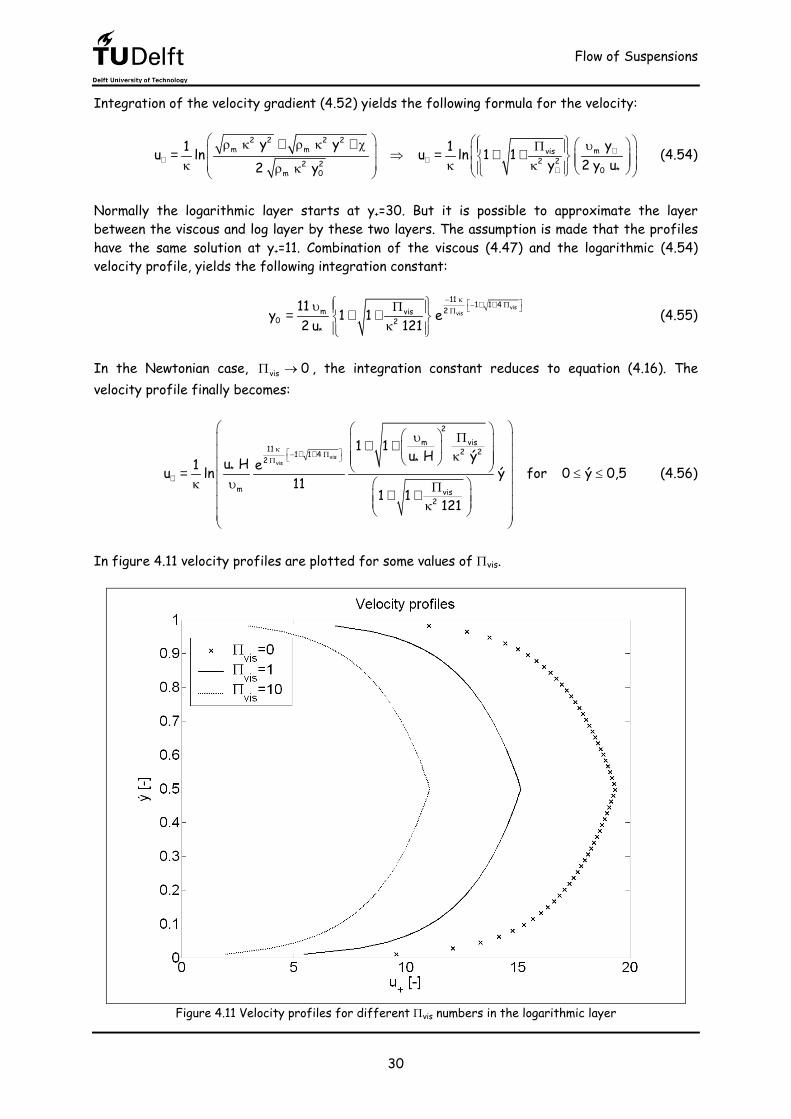
In figure 4.11 velocity profiles are plotted for some values of Πvis.
Figure 4.11 Velocity profiles for different Πvis numbers in the logarithmic layer
Flow of Suspensions
31
The velocity profile (4.56) reduces to equation (4.19) for the Newtonian case. It is clear that the velocity profile is shifted to the left when Πvis increases, because particle collisions are responsible for an increase in the skin friction. The shear stress in dimensionless form reads:
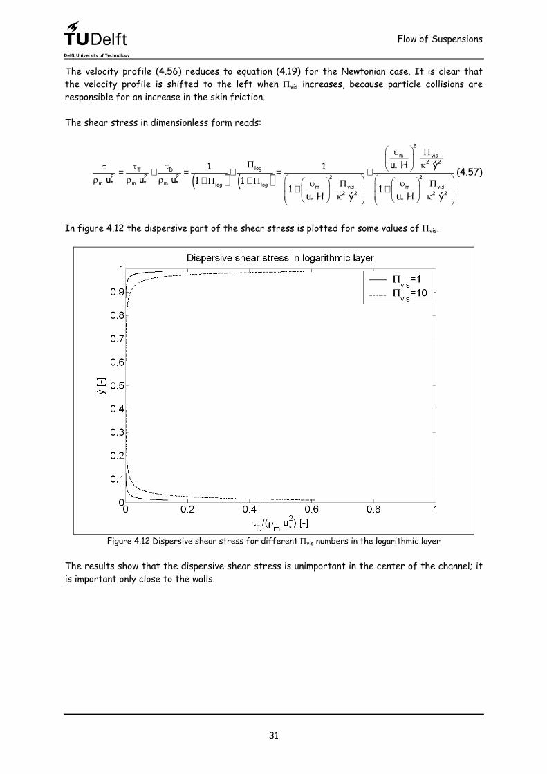
In figure 4.12 the dispersive part of the shear stress is plotted for some values of Πvis.
Figure 4.12 Dispersive shear stress for different Πvis numbers in the logarithmic layer
The results show that the dispersive shear stress is unimportant in the center of the channel; it is important only close to the walls.
Flow of Suspensions
32
4.6 Concentration profile An important dimensionless parameter to relate the particle response time τp to the flow field is the Stokes number, defined as the ratio between the particle response time and the hydrodynamic time scale τh: p
hSt τ
= τ (4.58) The hydrodynamic time scale can be constructed from the velocity scale U and the length scale L of the large-scale eddies. The typical velocity scale is u* and the maximum ratio between the velocity and length scale is about 2.5, see paragraph 8.1. The Stokes number then becomes: p p *
max puSt St St 2,5τ τ
= ⇒ = ⇒ ≈ τUL L (4.59)
For very large Stokes numbers the particles are not influenced by the flow fluctuations. The behaviour is dominated by bouncing against the walls and particle collisions. For small Stokes numbers the particles react almost instantaneously to velocity fluctuations. The particles will follow the flow almost perfectly.
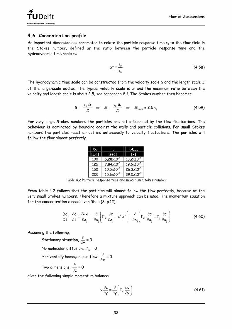
Table 4.2 Particle response time and maximum Stokes number From table 4.2 follows that the particles will almost follow the flow perfectly, because of the very small Stokes numbers. Therefore a mixture approach can be used. The momentum equation for the concentration c reads, van Rhee [8, p.12]: ∂∂ ∂ ∂ ∂ ∂ ∂= + = Γ − = Γ + Γ ∂ ∂ ∂ ∂ ∂ ∂ ∂
jm j m j
j j j j j j
c uDc c c c cc'u 'Dt t x x x x x x (4.60) Assuming the following,
gives the following simple momentum balance: ∂ ∂ ∂= Γ ∂ ∂ ∂ d
c cv y y y (4.61)
Flow of Suspensions
33
in which Γd is the eddy diffusivity coefficient. Assume that the eddy diffusivity is related to the eddy viscosity by: vdΓ = ϕ Γ (4.62) where ϕ is a constant of proportionality to relate the eddy diffusivity to eddy viscosity. At low concentrations 1ϕ � . For highly concentrated suspensions a value of 1,35ϕ � is used, Harris [24]. The vertical grain velocity v is equal to the settling velocity –vs. Integration of equation (4.61) leads to: ∂Γ + =∂ sd
c v c 0y (4.63) in which the integration constant is zero. The first term is transport due to turbulent diffusion and the last term is downward transport due to the settling of grains. For the eddie viscosity the parabolic distribution is used (4.31), because the 4th order distribution (4.30) gives not an analytical solution and the profile based on the logarithmic velocity (4.29) gives problems at the center of the channel, Γv=0. Combination of equation (4.63) and (4.31) results in the following differential equation: ( ) s
*
vcý 1 ý c 0ý u∂− + =∂ ϕ κ (4.64)
The solution of this differential equation reads:
Rous
4*
1-ý vc(ý) C with Rouý u
= = ϕ κ (4.65)
in which C4 is an integration constant and Rou is the Rouse parameter. Typically Rou<1 holds for profiles representing significantly suspended sediment loads. From now on Rou<1 is assumed for exploiting exact solutions. The depth-averaged concentration, the bulk concentration cb, can be found from the integration of equation (4.65):
= ∫Rou1
b 40
1-ýc C dýý (4.66) To get an answer a Beta function is used. The Beta function is defined as, Abramowitz [17, p.258]: ( ) ( ) ( ) ( )
( )− Γ Γ
= − Γ +∫1 w 1z-10
z wB z,w ý 1 ý dý= z w (4.67)
Flow of Suspensions
34
where Γ is the Gamma function. This Gamma function reads, Abramowitz [17, p.255]: ( )
∞−Γ = ∫ ý z-1
0z e ý dý (4.68)
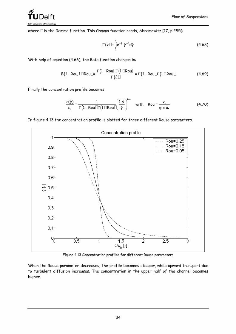
With help of equation (4.66), the Beta function changes in: ( ) ( ) ( )
In figure 4.13 the concentration profile is plotted for three different Rouse parameters.
Figure 4.13 Concentration profiles for different Rouse parameters
When the Rouse parameter decreases, the profile becomes steeper, while upward transport due to turbulent diffusion increases. The concentration in the upper half of the channel becomes higher.
Flow of Suspensions
35
4.7 Flux Richardson number The derivation of the extended velocity profile in paragraph 4.5 neglected the effect of buoyancy. This paragraph checks this assumption. Turbulent kinetic energy is needed to hold the particles in suspension. The shear stress produces this energy. The equation for turbulent kinetic energy is, Nieuwstadt [11, p.100]: S B
De P P TDt = − + − ε (4.71) in which:
e Turbulent kinetic energy, '2i
1e u2=
SP Shear production, 2
' ' i iS i j v,i
j j
u uP u u x x ∂ ∂
= − Γ ∂ ∂ ∼
BP Buoyancy production, ' ' mB j m j3 j3d,i
m m j
g gP u x − ∂ρ
= ρ δ Γ δ ρ ρ ∂ ∼
T Transport, ' ' ' 'j j m
j m j
1 eT u e p ux x ∂ ∂= − − + υ ∂ ρ ∂
ε Dissipation, 2'
im
j
ux
∂ε = υ ∂
The two interesting terms are the shear production term and the buoyancy term. The ratio between these two terms gives the flux Richardson number: B
S
buoyancy production PRi shear production P= = (4.72) A stable situation arises when this number is positive. This stable situation occurs in the sediment-laden flow situation, because of the negative concentration gradient, see figure 4.13. Neglecting the transport term gives for the turbulent kinetic energy equation (4.71): ( )S
De P 1 RiDt = − − ε (4.73) The turbulence will die when the Richardson number is larger than 1. From measurements follows that turbulence will already die when Ri>0.3 and that there is no damping when Ri<0.05, Uittenbogaard [personal communication] and Nieuwstadt [11, p.101]. The buoyancy production term can be written as, with help of equation (4.37) and (4.63): B
3 2* *
sp
P H g H Rouu u 1 1c(ý)
ϕ κ= + ρ
(4.74)
where c(ý) can be found from equation (4.70).
Flow of Suspensions
36
Manipulating the shear production term gives for the lower half of the channel, with help of equation (4.52) and (4.29): ( )
( ) ( )Sm pf3
* log
1 2 ýP H 1 1 with 1 c(ý) c(ý)u ý 1−
= ρ = ρ − + ρκ + Π (4.75)
The flux Richardson number can be computed by dividing the two production terms: ( )
( )2 log
2*
sp
1g H ýRi Rou u 1 2 ý1 1c(ý)
+Π ϕ κ= − + ρ
(4.76)
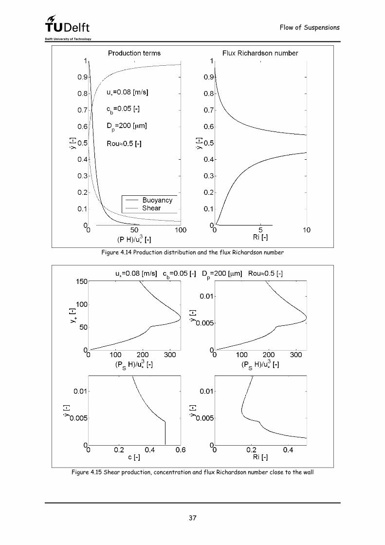
The flux Richardson number can be analysed only when transport due to turbulent diffusion and downward transport due to the settling of grains is in equilibrium, see equation (4.63). Another condition is that the transport term T must be small compared to the shear production term PS. Nieuwstadt [11, p.95] shows that these two terms are more or less equal at a value of y+=130. Above this value turbulent transport dominates over shear production. The only interesting region to analyse the Richardson number is thus very close to the wall. The largest value of the flux Richardson number gives the worst-case scenario. From equation (4.76) follows that a combination of a large Rouse parameter and a large value of c(ý≈0)=cn gives the largest flux Richardson number. A large Rouse parameter can be obtained from a small friction velocity and a large settling velocity; a big particle diameter and a low bulk concentration results in a large settling velocity. In figure 4.15 some parameters are shown. The flux Richardson number at the position where the transport and the shear production terms are equal is approximately 0,2. In this doom scenario the turbulence will be damped a little. For the other cases the effect of buoyancy is almost negligible.
Flow of Suspensions
37
Figure 4.14 Production distribution and the flux Richardson number
Figure 4.15 Shear production, concentration and flux Richardson number close to the wall
Flow of Suspensions
38
Experimental Set-up
39
5 Experimental Set-up This chapter gives a description of the experimental set-up, and the measured parameters.
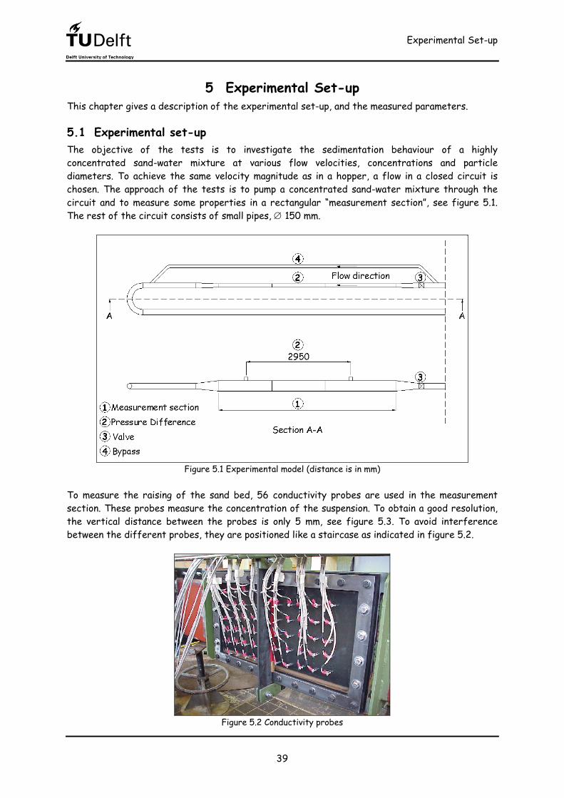
5.1 Experimental set-up The objective of the tests is to investigate the sedimentation behaviour of a highly concentrated sand-water mixture at various flow velocities, concentrations and particle diameters. To achieve the same velocity magnitude as in a hopper, a flow in a closed circuit is chosen. The approach of the tests is to pump a concentrated sand-water mixture through the circuit and to measure some properties in a rectangular “measurement section”, see figure 5.1. The rest of the circuit consists of small pipes, ∅ 150 mm.
Figure 5.1 Experimental model (distance is in mm) To measure the raising of the sand bed, 56 conductivity probes are used in the measurement section. These probes measure the concentration of the suspension. To obtain a good resolution, the vertical distance between the probes is only 5 mm, see figure 5.3. To avoid interference between the different probes, they are positioned like a staircase as indicated in figure 5.2.
Figure 5.2 Conductivity probes
Experimental Set-up
40
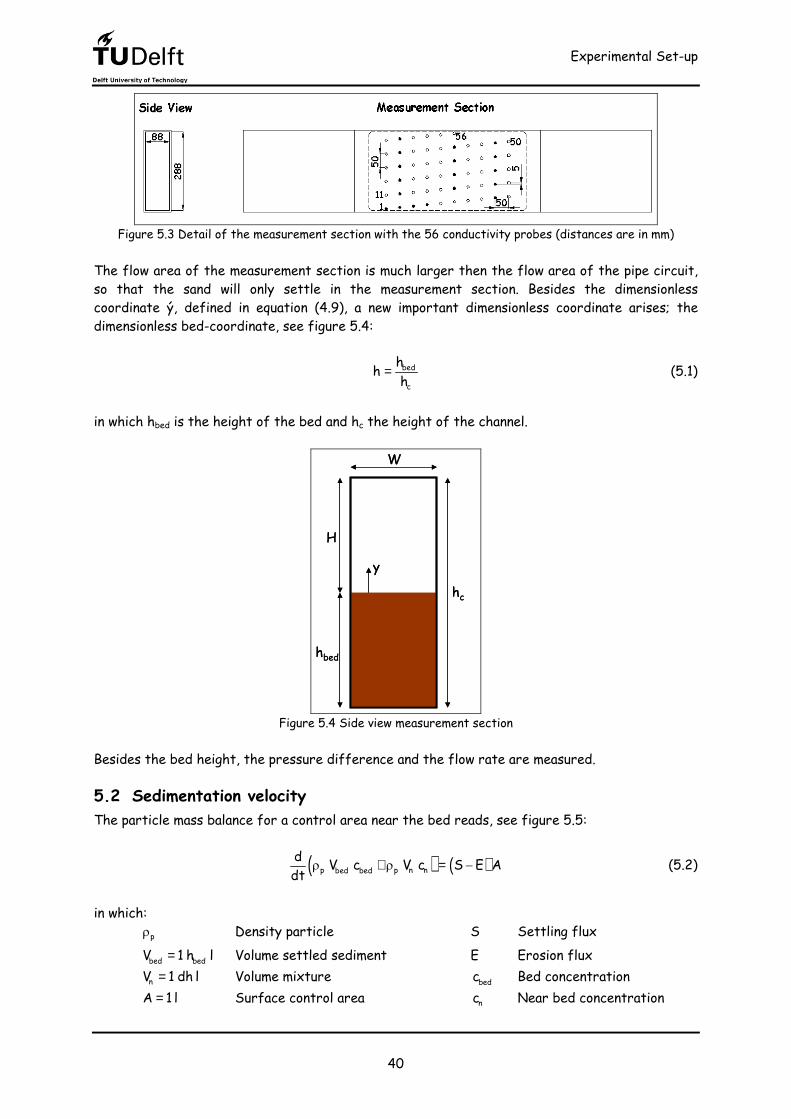
Figure 5.3 Detail of the measurement section with the 56 conductivity probes (distances are in mm) The flow area of the measurement section is much larger then the flow area of the pipe circuit, so that the sand will only settle in the measurement section. Besides the dimensionless coordinate ý, defined in equation (4.9), a new important dimensionless coordinate arises; the dimensionless bed-coordinate, see figure 5.4: bed
c
hh h= (5.1) in which hbed is the height of the bed and hc the height of the channel.
H
W
hbed
hc
yH
W
hbed
hc
y
Figure 5.4 Side view measurement section Besides the bed height, the pressure difference and the flow rate are measured.
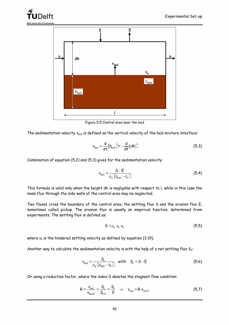
5.2 Sedimentation velocity The particle mass balance for a control area near the bed reads, see figure 5.5: ( ) ( )p p n nbed bed
d V c V c S E Adt ρ + ρ = − (5.2) in which:
pρ Density particle S Settling flux bed bedV 1 h l= Volume settled sediment E Erosion flux nV 1 dh l= Volume mixture bedc Bed concentration
A 1 l= Surface control area nc Near bed concentration
Experimental Set-up
41
u u
S E
vsed
cn
cbed
dh
l
hbed
u u
S E
vsed
cn
cbed
dh
l
hbed
Figure 5.5 Control area near the bed The sedimentation velocity vsed is defined as the vertical velocity of the bed-mixture interface: ( ) ( )sed bed
d dv h dhdt dt= = − (5.3) Combination of equation (5.2) and (5.3) gives for the sedimentation velocity: ( )sed
p nbed
S Ev c c−= ρ − (5.4)
This formula is valid only when the height dh is negligible with respect to l, while in this case the mass flux through the side walls of the control area may be neglected. Two fluxes cross the boundary of the control area; the settling flux S and the erosion flux E, sometimes called pickup. The erosion flux is usually an empirical function, determined from experiments. The settling flux is defined as: p n sS c v= ρ (5.5) where vs is the hindered settling velocity as defined by equation (3.19). Another way to calculate the sedimentation velocity is with the help of a net settling flux Sn: ( )
nnsed
p nbed
Sv with S S Ec c= = −ρ − (5.6) Or using a reduction factor, where the index 0 denotes the stagnant flow condition: sed n n
sed sed,0n,0sed,0
v S SR v R vv S S= = = ⇒ = (5.7)
Experimental Set-up
42
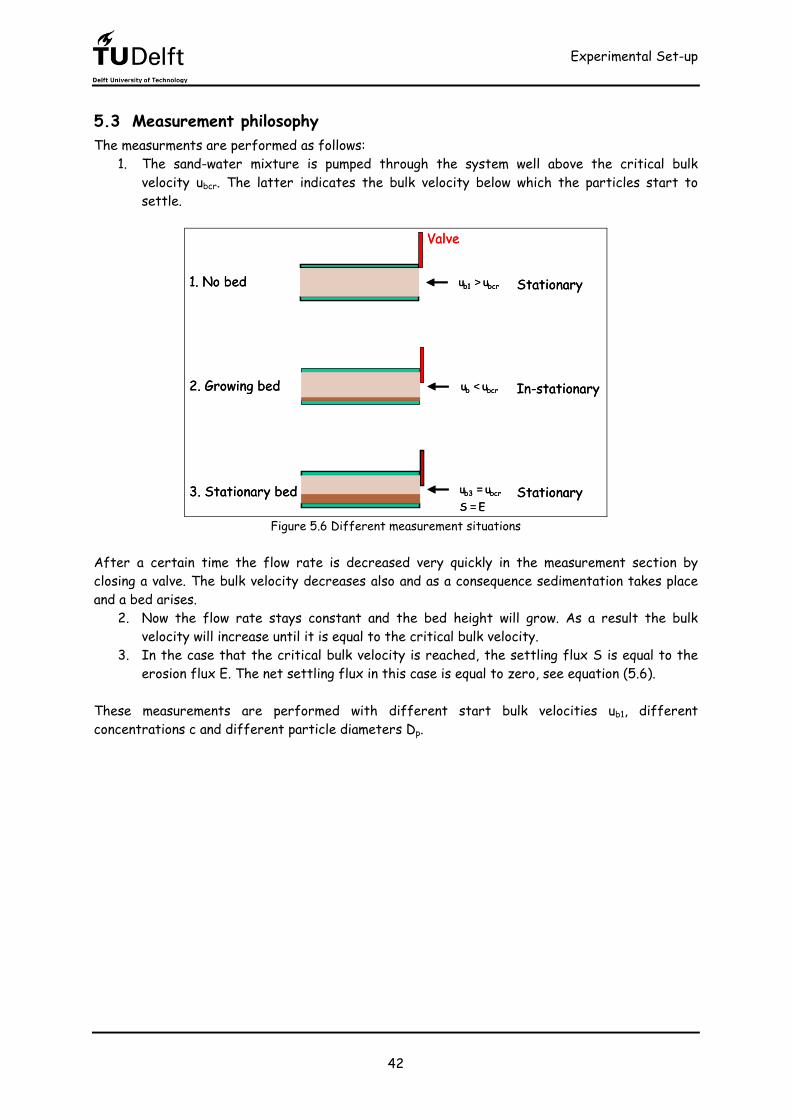
5.3 Measurement philosophy The measurments are performed as follows:
1. The sand-water mixture is pumped through the system well above the critical bulk velocity ubcr. The latter indicates the bulk velocity below which the particles start to settle.
b bcru u<2. Growing bed In-stationary
3. Stationary bed b3 bcru u= StationaryS E=
Stationaryb1 bcru u>1. No bed
Valve
b bcru u<2. Growing bed In-stationary
3. Stationary bed b3 bcru u= StationaryS E=
Stationaryb1 bcru u>1. No bed
Valve
Figure 5.6 Different measurement situations After a certain time the flow rate is decreased very quickly in the measurement section by closing a valve. The bulk velocity decreases also and as a consequence sedimentation takes place and a bed arises.
2. Now the flow rate stays constant and the bed height will grow. As a result the bulk velocity will increase until it is equal to the critical bulk velocity.
3. In the case that the critical bulk velocity is reached, the settling flux S is equal to the erosion flux E. The net settling flux in this case is equal to zero, see equation (5.6).
These measurements are performed with different start bulk velocities ub1, different concentrations c and different particle diameters Dp.
Experimental Set-up
43
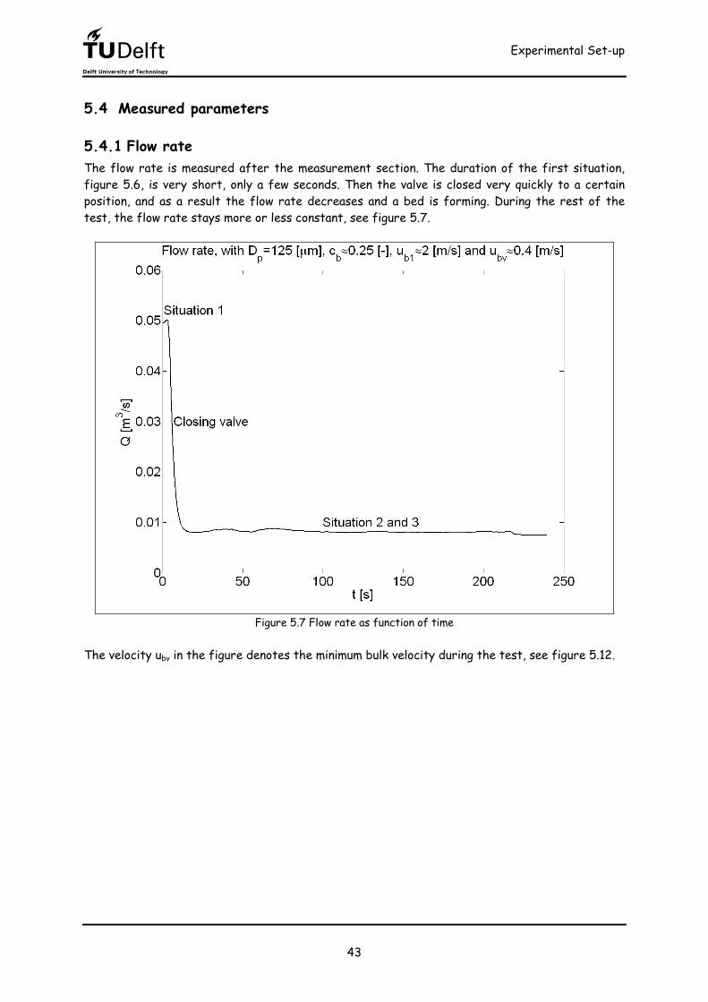
5.4 Measured parameters 5.4.1 Flow rate The flow rate is measured after the measurement section. The duration of the first situation, figure 5.6, is very short, only a few seconds. Then the valve is closed very quickly to a certain position, and as a result the flow rate decreases and a bed is forming. During the rest of the test, the flow rate stays more or less constant, see figure 5.7.
Figure 5.7 Flow rate as function of time
The velocity ubv in the figure denotes the minimum bulk velocity during the test, see figure 5.12.
Experimental Set-up
44
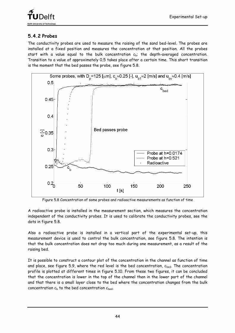
5.4.2 Probes The conductivity probes are used to measure the raising of the sand bed-level. The probes are installed at a fixed position and measures the concentration at that position. All the probes start with a value equal to the bulk concentration cb; the depth-averaged concentration. Transition to a value of approximately 0,5 takes place after a certain time. This short transition is the moment that the bed passes the probe, see figure 5.8.
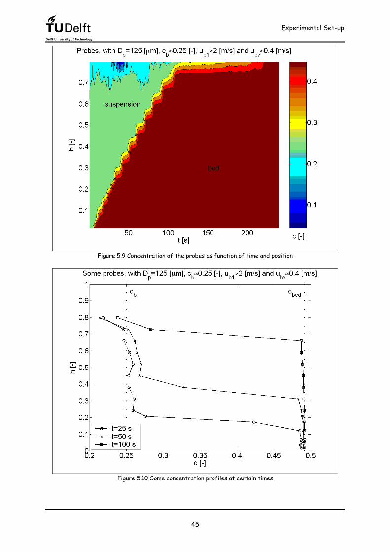
Figure 5.8 Concentration of some probes and radioactive measurements as function of time A radioactive probe is installed in the measurement section, which measures the concentration independent of the conductivity probes. It is used to calibrate the conductivity probes, see the dots in figure 5.8. Also a radioactive probe is installed in a vertical part of the experimental set-up, this measurement device is used to control the bulk concentration, see figure 5.8. The intention is that the bulk concentration does not drop too much during one measurement, as a result of the raising bed. It is possible to construct a contour plot of the concentration in the channel as function of time and place, see figure 5.9, where the red level is the bed concentration, cbed. The concentration profile is plotted at different times in figure 5.10. From these two figures, it can be concluded that the concentration is lower in the top of the channel then in the lower part of the channel and that there is a small layer close to the bed where the concentration changes from the bulk concentration cb to the bed concentration cbed.
Experimental Set-up
45
Figure 5.9 Concentration of the probes as function of time and position
Figure 5.10 Some concentration profiles at certain times
Experimental Set-up
46
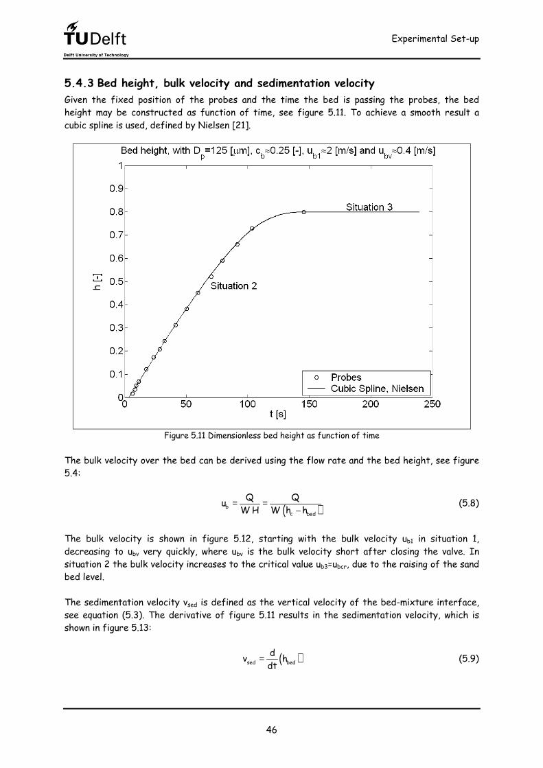
5.4.3 Bed height, bulk velocity and sedimentation velocity Given the fixed position of the probes and the time the bed is passing the probes, the bed height may be constructed as function of time, see figure 5.11. To achieve a smooth result a cubic spline is used, defined by Nielsen [21].
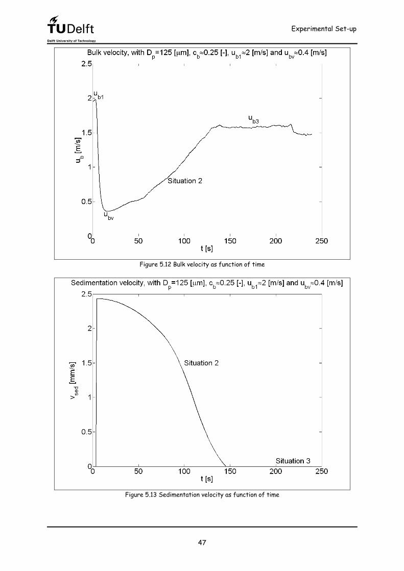
Figure 5.11 Dimensionless bed height as function of time The bulk velocity over the bed can be derived using the flow rate and the bed height, see figure 5.4: ( )b
c bed
Q Qu W H W h h= = − (5.8) The bulk velocity is shown in figure 5.12, starting with the bulk velocity ub1 in situation 1, decreasing to ubv very quickly, where ubv is the bulk velocity short after closing the valve. In situation 2 the bulk velocity increases to the critical value ub3=ubcr, due to the raising of the sand bed level. The sedimentation velocity vsed is defined as the vertical velocity of the bed-mixture interface, see equation (5.3). The derivative of figure 5.11 results in the sedimentation velocity, which is shown in figure 5.13: ( )sed bed
dv hdt= (5.9)
Experimental Set-up
47
Figure 5.12 Bulk velocity as function of time
Figure 5.13 Sedimentation velocity as function of time
Experimental Set-up
48
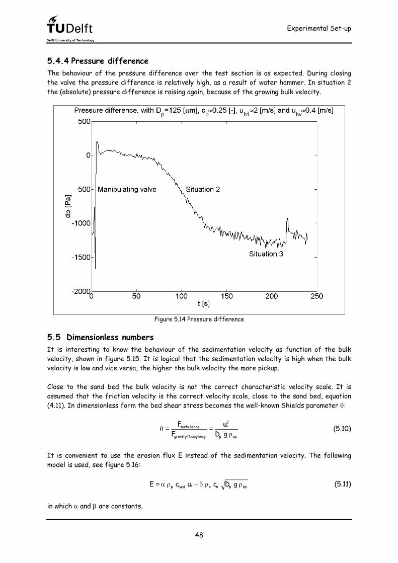
5.4.4 Pressure difference The behaviour of the pressure difference over the test section is as expected. During closing the valve the pressure difference is relatively high, as a result of water hammer. In situation 2 the (absolute) pressure difference is raising again, because of the growing bulk velocity.
Figure 5.14 Pressure difference
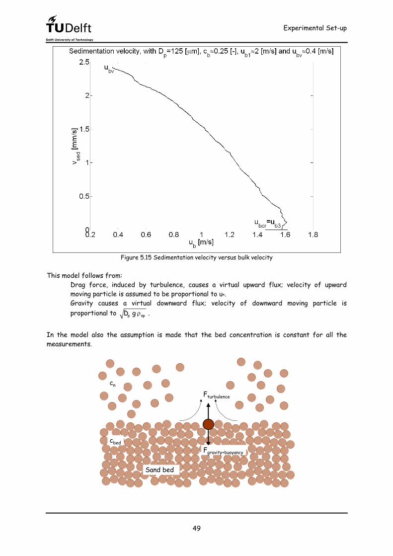
5.5 Dimensionless numbers It is interesting to know the behaviour of the sedimentation velocity as function of the bulk velocity, shown in figure 5.15. It is logical that the sedimentation velocity is high when the bulk velocity is low and vice versa, the higher the bulk velocity the more pickup. Close to the sand bed the bulk velocity is not the correct characteristic velocity scale. It is assumed that the friction velocity is the correct velocity scale, close to the sand bed, equation (4.11). In dimensionless form the bed shear stress becomes the well-known Shields parameter θ:
2turbulence *
p spgravity buoyancy
F uF D g+
θ = = ρ (5.10) It is convenient to use the erosion flux E instead of the sedimentation velocity. The following model is used, see figure 5.16: p p n p sp*bedE c u c D g= α ρ − β ρ ρ (5.11) in which α and β are constants.
Experimental Set-up
49
Figure 5.15 Sedimentation velocity versus bulk velocity This model follows from:
• Drag force, induced by turbulence, causes a virtual upward flux; velocity of upward moving particle is assumed to be proportional to u*.
• Gravity causes a virtual downward flux; velocity of downward moving particle is proportional to p spD g ρ .
In the model also the assumption is made that the bed concentration is constant for all the measurements.
Sand bed
Fturbulence
Fgravity+buoyancycbed
cn
Sand bed
Fturbulence
Fgravity+buoyancycbed
cn
Figure 5.16 Balance for dimensionless pickup
Experimental Set-up
50
The dimensionless pickup is, with help of (5.11): bed
pnp n p sp
cEcc D g
ϕ = = α θ − β ρ ρ (5.12)
Einstein derived the following pickup [8, p.85]: p
p p sp
ED gφ = ρ ρ (5.13)
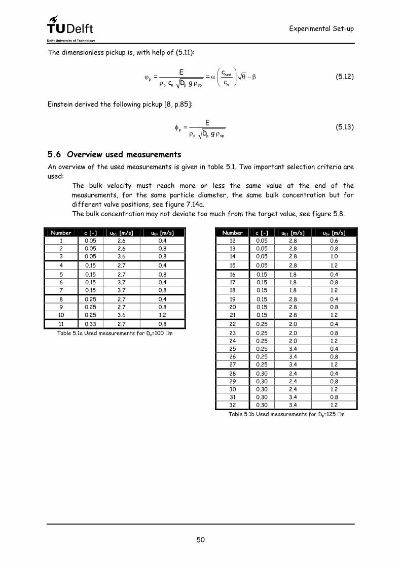
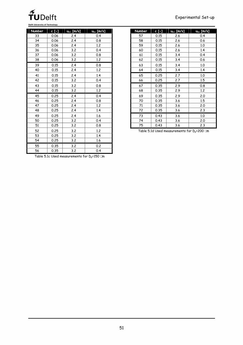
5.6 Overview used measurements An overview of the used measurements is given in table 5.1. Two important selection criteria are used:
• The bulk velocity must reach more or less the same value at the end of the measurements, for the same particle diameter, the same bulk concentration but for different valve positions, see figure 7.14a.
• The bulk concentration may not deviate too much from the target value, see figure 5.8. Number c [-] ub1 [m/s] ubv [m/s] Number c [-] ub1 [m/s] ubv [m/s]
Experimental Results on Sedimentation in Stagnant Flow
53
6 Experimental Results on Sedimentation in Stagnant Flow In this chapter the results are shown for the case that there is only a settling flux, no erosion.
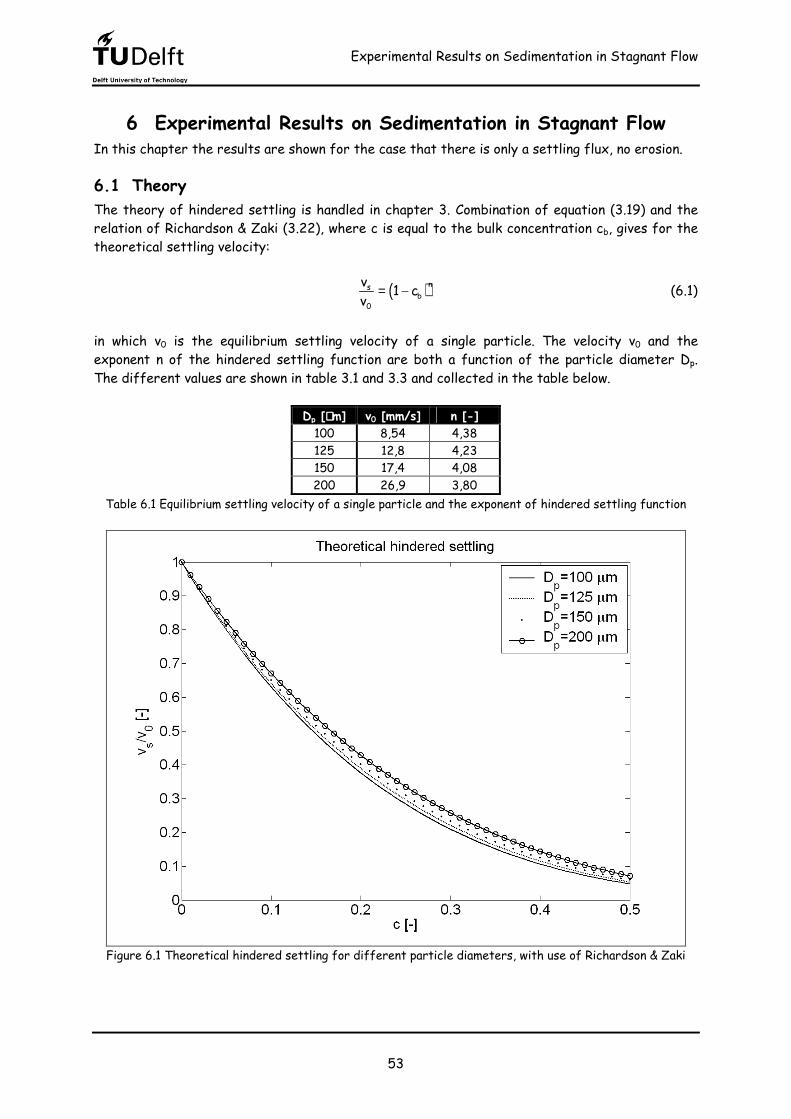
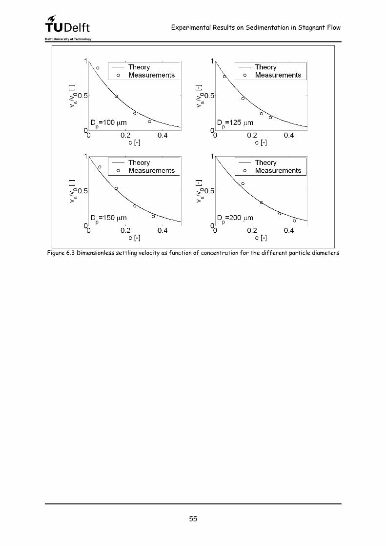
6.1 Theory The theory of hindered settling is handled in chapter 3. Combination of equation (3.19) and the relation of Richardson & Zaki (3.22), where c is equal to the bulk concentration cb, gives for the theoretical settling velocity: ( )ns
b0
v 1 cv = − (6.1) in which v0 is the equilibrium settling velocity of a single particle. The velocity v0 and the exponent n of the hindered settling function are both a function of the particle diameter Dp. The different values are shown in table 3.1 and 3.3 and collected in the table below.
Dp [µµµµm] v0 [mm/s] n [-] 100 8,54 4,38
125 12,8 4,23
150 17,4 4,08
200 26,9 3,80
Table 6.1 Equilibrium settling velocity of a single particle and the exponent of hindered settling function
Figure 6.1 Theoretical hindered settling for different particle diameters, with use of Richardson & Zaki
Experimental Results on Sedimentation in Stagnant Flow
54
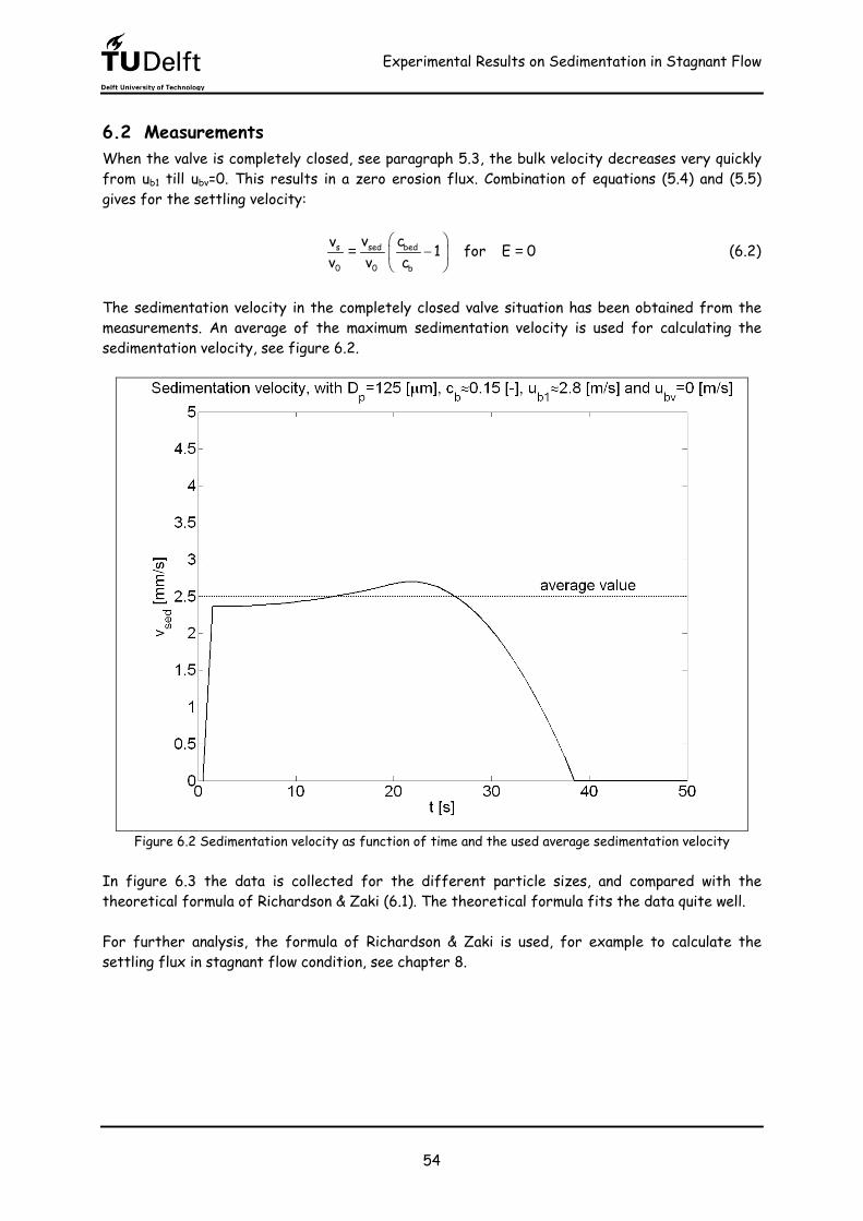
6.2 Measurements When the valve is completely closed, see paragraph 5.3, the bulk velocity decreases very quickly from ub1 till ubv=0. This results in a zero erosion flux. Combination of equations (5.4) and (5.5) gives for the settling velocity: s sed bed
0 0 b
v cv 1 for E 0v v c
= − = (6.2)
The sedimentation velocity in the completely closed valve situation has been obtained from the measurements. An average of the maximum sedimentation velocity is used for calculating the sedimentation velocity, see figure 6.2.
Figure 6.2 Sedimentation velocity as function of time and the used average sedimentation velocity
In figure 6.3 the data is collected for the different particle sizes, and compared with the theoretical formula of Richardson & Zaki (6.1). The theoretical formula fits the data quite well. For further analysis, the formula of Richardson & Zaki is used, for example to calculate the settling flux in stagnant flow condition, see chapter 8.
Experimental Results on Sedimentation in Stagnant Flow
55
Figure 6.3 Dimensionless settling velocity as function of concentration for the different particle diameters
Experimental Results on Sedimentation in Stagnant Flow
56
Bed Shear Stress
57
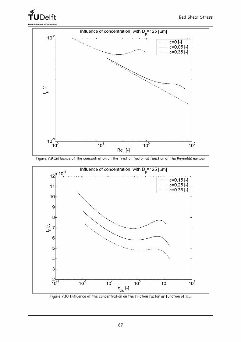
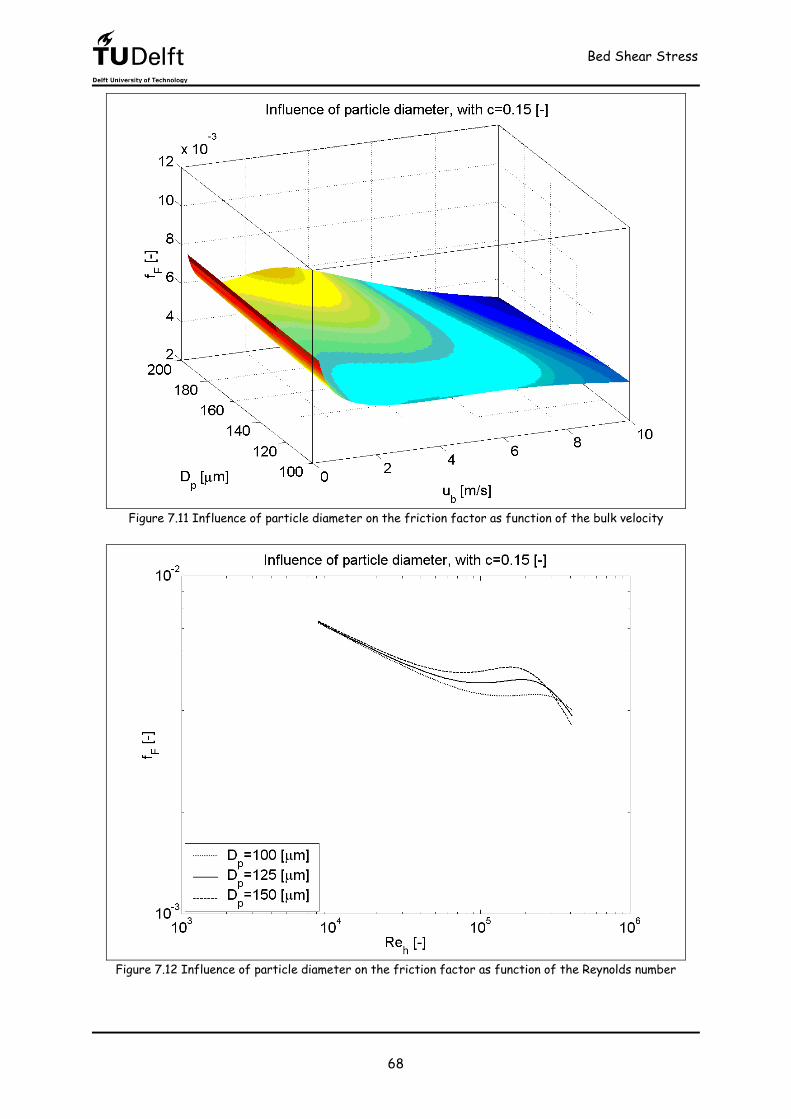
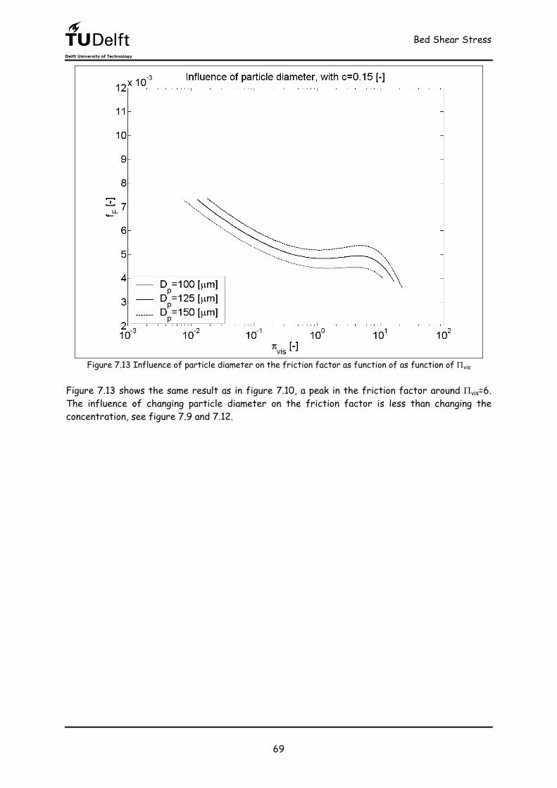
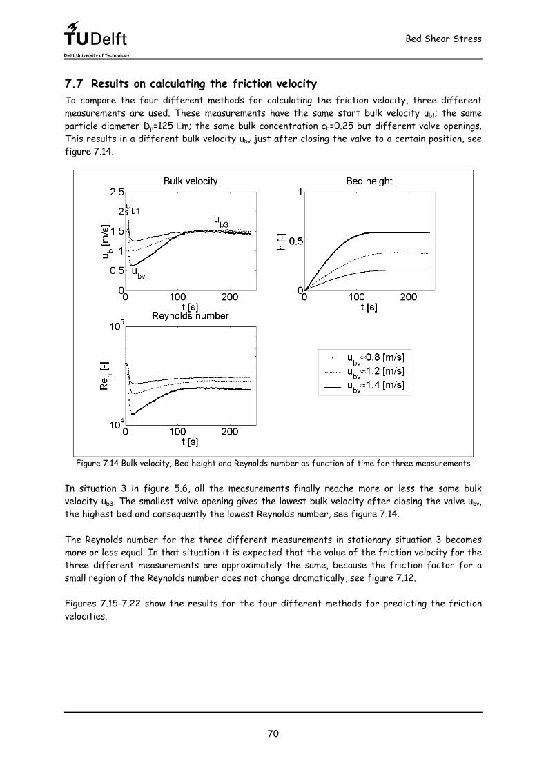
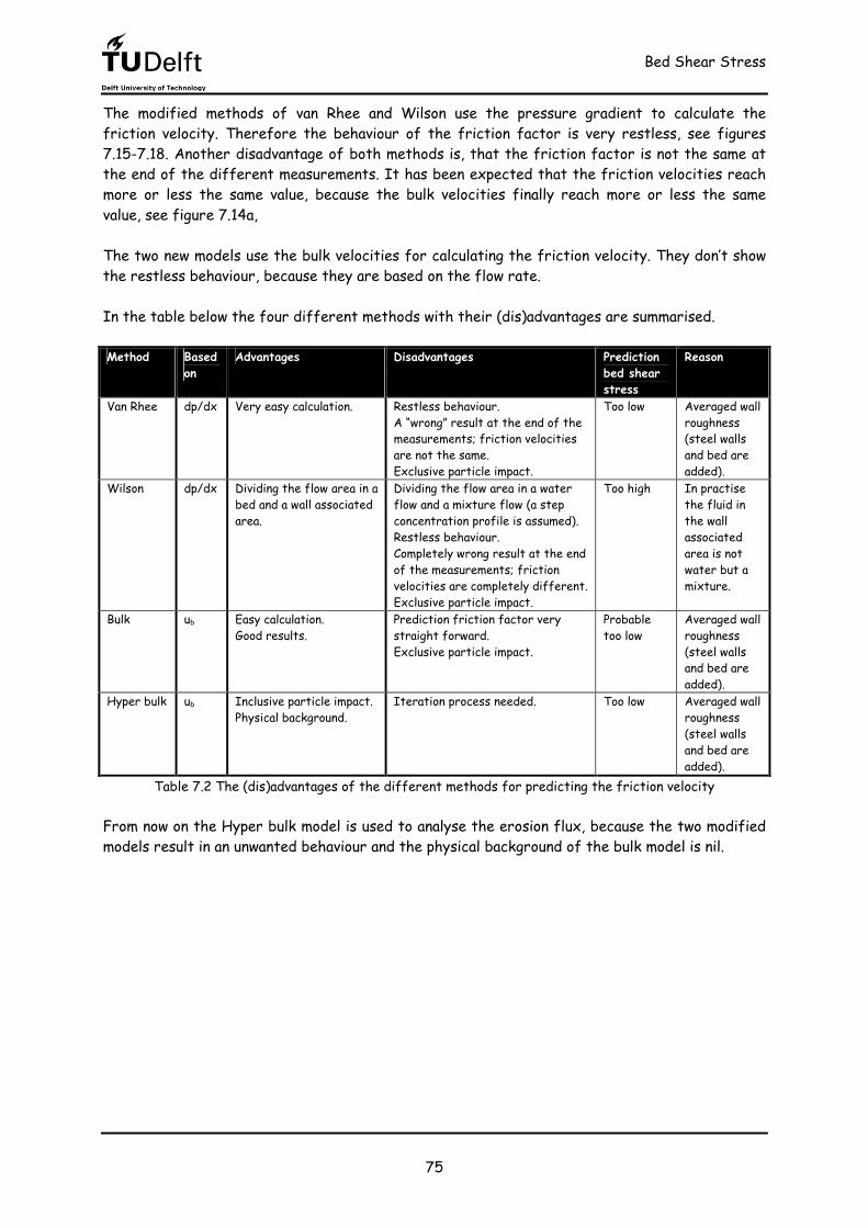
7 Bed Shear Stress This chapter gives two existing and two new models for calculating the pressure gradient.
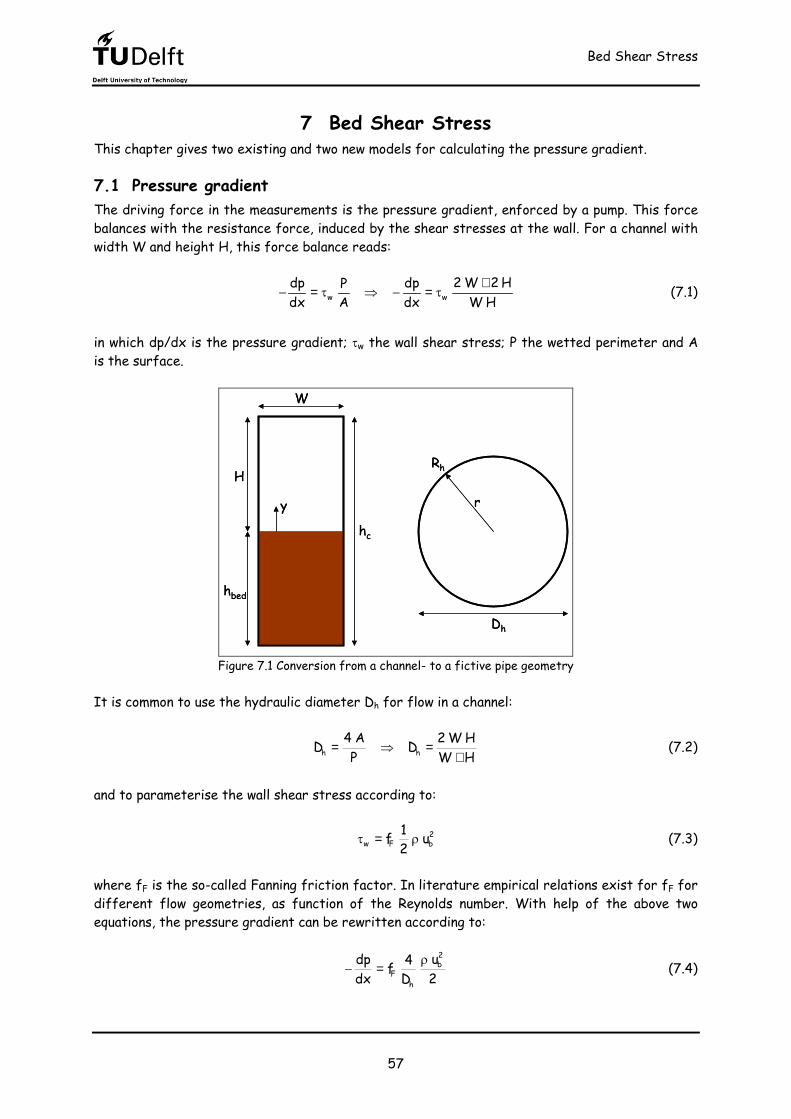
7.1 Pressure gradient The driving force in the measurements is the pressure gradient, enforced by a pump. This force balances with the resistance force, induced by the shear stresses at the wall. For a channel with width W and height H, this force balance reads: w w
2 W 2 Hdp dpPdx A dx W H
+− = τ ⇒ − = τ (7.1) in which dp/dx is the pressure gradient; τw the wall shear stress; P the wetted perimeter and A is the surface.
Dh
r
RhH
W
hbed
hc
y
Dh
r
RhH
W
hbed
hc
y
Figure 7.1 Conversion from a channel- to a fictive pipe geometry
It is common to use the hydraulic diameter Dh for flow in a channel: h h
4 A 2 W HD DP W H= ⇒ =+
(7.2) and to parameterise the wall shear stress according to: 2
w F b1f u2τ = ρ (7.3)
where fF is the so-called Fanning friction factor. In literature empirical relations exist for fF for different flow geometries, as function of the Reynolds number. With help of the above two equations, the pressure gradient can be rewritten according to:
2b
Fh
udp 4fdx D 2ρ− = (7.4)
Bed Shear Stress
58
where the Reynolds number Reh is based on the hydraulic diameter and the bulk velocity: b h
hu DRe = υ (7.5)
7.2 Friction factor When the pressure gradient, bulk velocity and the hydraulic diameter are known, the friction factor can be computed from equation (7.4): h
F 2b
Ddpf dx 2 u
= − ρ (7.6)
7.2.1 Laminar flow To calculate the friction factor, it is necessary to know the velocity distribution. This velocity distribution for laminar fully developed flow in a pipe is given by, White [21, p.341]: ( ) ( )2 2
hdp1u r R r4 dx
= − − µ (7.7)
For further calculations it is necessary to know the bulk velocity. Integrating the velocity over the whole pipe diameter gives the bulk velocity:
( )
hR2h0
b b2h
u r 2 r dr R dpQu uA R 8 dxπ
= = ⇒ = − π µ ∫
(7.8) Combination of equation (7.6) and the calculated bulk velocity results in the friction factor for flow in a laminar situation: F
h
16f Re= (7.9) For industrial flows, transition takes place at Reh≈2100 and hence (7.9) is valid only for Reh<2100.
7.2.2 Turbulent flow With the definition of the wall shear stress from equation (7.3) and equation (4.7), the friction factor for turbulent flow becomes:
22 2 *
F Fb*b
u1u f u f 22 u ρ = ρ ⇒ =
(7.10) Calculating the bulk velocity in the case that a logarithmic profile is used, give problems close to the wall. Therefore the power-law approximation (4.21) is used as approximation for a turbulent velocity profile, see figure 4.3:
1 8 1 17 7 7 73b * h14 1u C u D15 2
− = υ (7.11)
Bed Shear Stress
59
Combination of the equations (7.10) and (7.11) yields for the friction factor:
75 7 1 7 144 4 4 4 4F 3 F 3h h14f 2 C Re f 2,684 C Re15
− − − − − = ⇒ = (7.12) For the constant in this equation, several values are used. A well-known friction factor is the one from Blasius [21, p.345] for smooth pipe flow:
13 54F h hf 0,079 Re for 4 10 Re 10−
= ⋅ < < (7.13) and for duct flow, Dean [22]:
13 54F h hf 0,073 Re for 6 10 Re 6 10−
= ⋅ < < ⋅ (7.14)
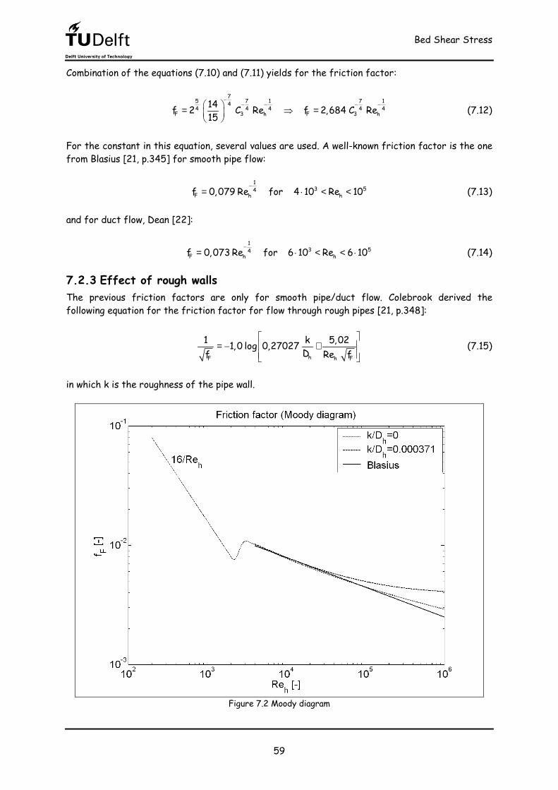
7.2.3 Effect of rough walls The previous friction factors are only for smooth pipe/duct flow. Colebrook derived the following equation for the friction factor for flow through rough pipes [21, p.348]:
hF Fh
1 k 5,021,0 log 0,27027 Df Re f = − +
(7.15) in which k is the roughness of the pipe wall.
Figure 7.2 Moody diagram
Bed Shear Stress
60
Stuart [23] derives a single correlation for the friction loss to Reynolds number roughness for laminar, transitional and turbulent flow:
( )
1610,91
12 12 h h1,5F
h 16
h
7 kA 2, 457 ln 0,27Re D8f 2 A B withRe37530B Re
−
−
= + = + + =
(7.16)
7.3 Modification of van Rhee’s model The model of “van Rhee” calculated the bed shear stress directly from the pressure gradient: h
bed,van Rhee bed,van RheeW H Ddp dp
dx 2 W 2 H dx 4 τ = − ⇒ τ = − + (7.17)
The friction velocity can thus be calculated from: h
*van Rheem
Ddpu dx 4
= − ρ (7.18)
The advantage of this model is the very easy calculation of the friction velocity with the known dimensions and the measured pressure drop. The disadvantage of the model is that the calculated friction velocity is an average value. The roughness of the bottom (bed) and the other walls (steel) are different, so that the prediction of the bed shear stress or the friction velocity is too low, see figure 7.1.
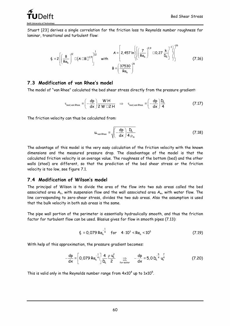
7.4 Modification of Wilson’s model The principal of Wilson is to divide the area of the flow into two sub areas called the bed associated area Ab, with suspension flow and the wall associated area Aw, with water flow. The line corresponding to zero-shear stress, divides the two sub areas. Also the assumption is used that the bulk velocity in both sub areas is the same. The pipe wall portion of the perimeter is essentially hydraulically smooth, and thus the friction factor for turbulent flow can be used. Blasius gives for flow in smooth pipes (7.13):
13 54F h hf 0,079 Re for 4 10 Re 10−
= ⋅ < < (7.19) With help of this approximation, the pressure gradient becomes: �
21 5 7b4 4 4bh h
for waterh
udp dp40,079 Re 5,0 D udx D 2 dx− − ρ− = ⇒ − =
(7.20) This is valid only in the Reynolds number range from 4x10⁴ up to 1x10⁵.
Bed Shear Stress
61
Dw
Ab
Db
ρm
AwρwDw
Ab
Db
ρm
Awρw
Figure 7.3 Principal of Wilson Solving (7.20) results in the following hydraulic diameter of the wall-associated area:
4 75 5w bhdpD D 3,62 udx
− = = − (7.21)
When the diameter is known, it is easy to calculate the surface of the wall-associated area with: ( )ww
w ww
D W 2 H4 AD AP 4+
= ⇒ = (7.22) After that it is possible to derive the bed associated area: ( )w
wb bD W 2 HA A A A W H 4
+= − ⇒ = − (7.23)
and the corresponding hydraulic diameter: b
wb bb
4 A 2 HD D 4 H D 1P W = ⇒ = − + (7.24)
Finally the bed shear stress becomes: b b
bed,Wilson bed,Wilsonb
dp dpA Ddx P dx 4
τ = − ⇒ τ = − (7.25) and the corresponding friction velocity: b
*Wilsonm
dp Du dx 4
= − ρ (7.26)
Bed Shear Stress
62
The advantage of Wilson’s model is the dividing of the flow area into two areas, one associated with the wall and the other with the bed. This method aims to determine the friction velocity from the friction caused by the presence of the bed alone. The disadvantage of this model is, that it may lead to physically unrealistic results; for some measurements the calculated wall associated area is larger then the total flow area?
7.5 Bulk model The bulk model calculates the friction velocity directly from the bulk velocity (7.10): F
b*Bulkfu u2= (7.27)
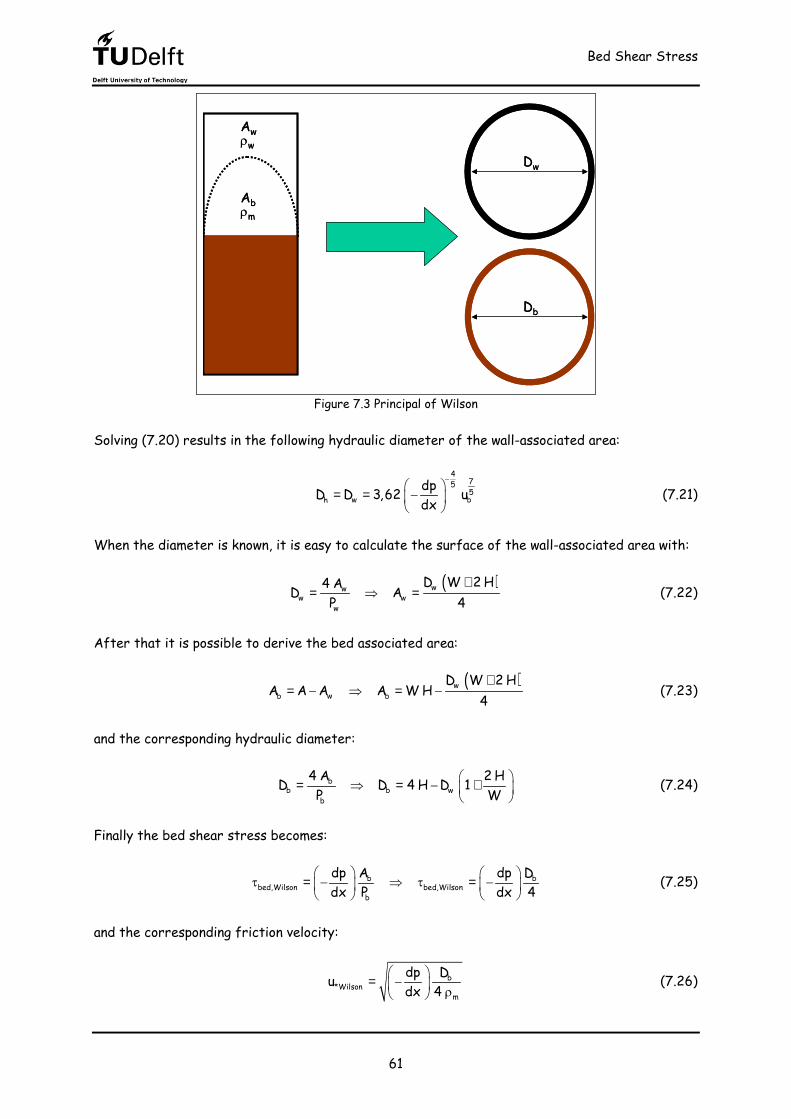
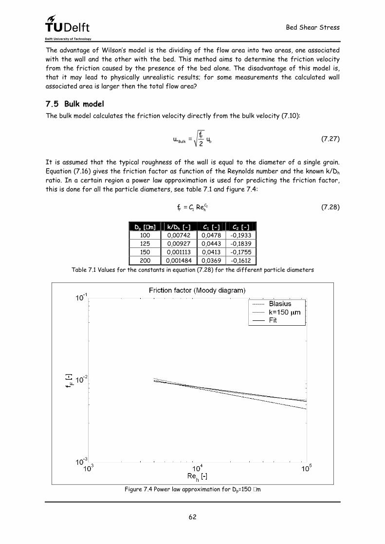
It is assumed that the typical roughness of the wall is equal to the diameter of a single grain. Equation (7.16) gives the friction factor as function of the Reynolds number and the known k/Dh ratio. In a certain region a power law approximation is used for predicting the friction factor, this is done for all the particle diameters, see table 7.1 and figure 7.4: 2C
Table 7.1 Values for the constants in equation (7.28) for the different particle diameters
Figure 7.4 Power law approximation for Dp=150 µm
Bed Shear Stress
63
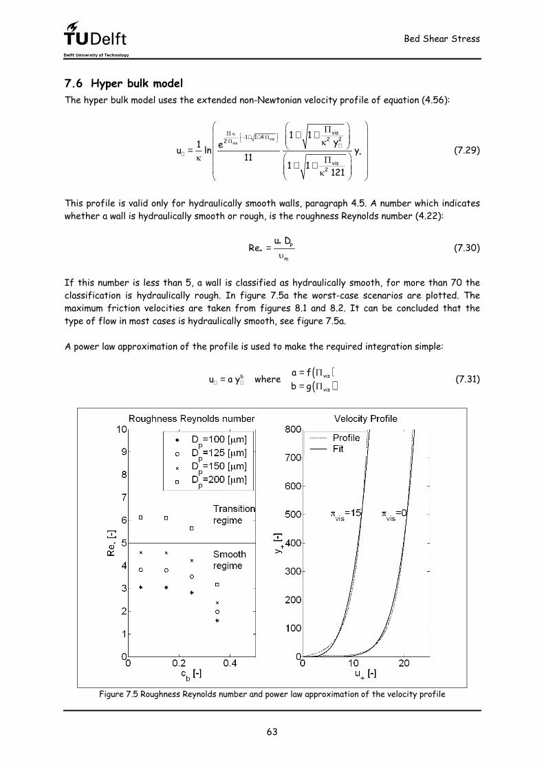
7.6 Hyper bulk model The hyper bulk model uses the extended non-Newtonian velocity profile of equation (4.56):
visvis
vis11 1 1 4 2 22+
vis2
1 1 y1 eu ln y11 1 1 121
κ − + + Π Π+
+
Π + + κ = κ Π + + κ
(7.29)
This profile is valid only for hydraulically smooth walls, paragraph 4.5. A number which indicates whether a wall is hydraulically smooth or rough, is the roughness Reynolds number (4.22): p*
*m
u DRe = υ (7.30) If this number is less than 5, a wall is classified as hydraulically smooth, for more than 70 the classification is hydraulically rough. In figure 7.5a the worst-case scenarios are plotted. The maximum friction velocities are taken from figures 8.1 and 8.2. It can be concluded that the type of flow in most cases is hydraulically smooth, see figure 7.5a. A power law approximation of the profile is used to make the required integration simple: ( )
( )visbvis
a fu a y where b g+ +
= Π=
= Π (7.31)
Figure 7.5 Roughness Reynolds number and power law approximation of the velocity profile
Bed Shear Stress
64
The coefficients of the power law are approximated by the following function: ( )
C43 visCvis 1 2f C C e ΠΠ = + (7.32)
After calculating, the power law coefficients read: ( )
( )
0,523vis
0,09vis
0,697vis
4,24vis
a f 1,76 6,67 eb g 0,138 3,74 e −
− Π
− Π= Π = +
= Π = + (7.33)
The coefficients are shown in figure 7.6. In the Newtonian case both values returns back to the well-known values of the Newtonian power law approximation, see paragraph 4.2.1. About 8.5 for the first constant and 1/7 (≈0.143) for the second.
Figure 7.6 Approximation of coefficients a and b in equation (7.31) Finally the power law approximation of the extended velocity profile (4.56) becomes:
0,523vis
0,09vis
0,697b
4,24a 1,76 6,67 eu a y with b 0,138 3,74 e
− Π
+ + − Π= +
== +
(7.34) A 3-d plot of the velocity profile is shown in figure 7.7, as function of the dimensionless coordinate y+ and the dimensionless number ∏vis. The velocity profile changes most when ∏vis is between 0 and 5.
Bed Shear Stress
65
Figure 7.7 Velocity profile as function of y+ and ∏vis To calculate the friction factor, it is necessary to know the bulk velocity. The bulk velocity can be calculated from the integration of the velocity profile:
( )
h
h
Rb R
b 1*0 *b b2 2
mh h 0
u r 2 r dr 2 a u uQu u r drA R R+
π = = ⇒ = π υ
∫ ∫ (7.35) The solution is: ( )
( )
( )*b u* * * h
bm*
2 a u u u Du b u 2 2
= + υ (7.36)
An iteration process is needed to solve this equation with respect to u*. The coefficients of the power law are a function of ∏vis and thus of u*, see equation (4.46). At least the formula can be solved with an iteration process to: ( )pb*u f u ,c,D= (7.37) where u* is then a function of the known bulk velocity; the known bulk concentration and the known particle diameter.
Bed Shear Stress
66
In figure 7.8 the friction factor is plotted as function of the volumetric fraction c.
Figure 7.8 Influence of the concentration on the friction factor as function of the bulk velocity
The friction factor shows a strange peak around Πvis=6, see figure 7.9 and 7.10. In that situation is: ( )F
vis
d f 0d =Π (7.38) This peak is probably a disadvantage of the chosen method. The friction factor after the peak decreases faster than before the peak. In figure 7.11 the friction factor is plotted as function of the particle diameter Dp.
Bed Shear Stress
67
Figure 7.9 Influence of the concentration on the friction factor as function of the Reynolds number
Figure 7.10 Influence of the concentration on the friction factor as function of Πvis
Bed Shear Stress
68
Figure 7.11 Influence of particle diameter on the friction factor as function of the bulk velocity
Figure 7.12 Influence of particle diameter on the friction factor as function of the Reynolds number
Bed Shear Stress
69
Figure 7.13 Influence of particle diameter on the friction factor as function of as function of Πvis Figure 7.13 shows the same result as in figure 7.10, a peak in the friction factor around Πvis=6. The influence of changing particle diameter on the friction factor is less than changing the concentration, see figure 7.9 and 7.12.
Bed Shear Stress
70
7.7 Results on calculating the friction velocity To compare the four different methods for calculating the friction velocity, three different measurements are used. These measurements have the same start bulk velocity ub1; the same particle diameter Dp=125 µm; the same bulk concentration cb=0.25 but different valve openings. This results in a different bulk velocity ubv just after closing the valve to a certain position, see figure 7.14.
Figure 7.14 Bulk velocity, Bed height and Reynolds number as function of time for three measurements In situation 3 in figure 5.6, all the measurements finally reache more or less the same bulk velocity ub3. The smallest valve opening gives the lowest bulk velocity after closing the valve ubv, the highest bed and consequently the lowest Reynolds number, see figure 7.14. The Reynolds number for the three different measurements in stationary situation 3 becomes more or less equal. In that situation it is expected that the value of the friction velocity for the three different measurements are approximately the same, because the friction factor for a small region of the Reynolds number does not change dramatically, see figure 7.12. Figures 7.15-7.22 show the results for the four different methods for predicting the friction velocities.
Bed Shear Stress
71
Figure 7.15 Friction velocity as function of time, based on van Rhee’s method
Figure 7.16 Sedimentation velocity as function of the friction velocity, based on van Rhee’s method
Bed Shear Stress
72
Figure 7.17 Friction velocity as function of time, based on van Wilson’s method
Figure 7.18 Sedimentation velocity as function of the friction velocity, based on van Wilson’s method
Bed Shear Stress
73
Figure 7.19 Friction velocity as function of time, based on the Bulk model
Figure 7.20 Sedimentation velocity as function of the friction velocity, based on the Bulk model
Bed Shear Stress
74
Figure 7.21 Friction velocity as function of time, based on the Hyper bulk model
Figure 7.22 Sedimentation velocity as function of the friction velocity, based on the Hyper bulk model
Bed Shear Stress
75
The modified methods of van Rhee and Wilson use the pressure gradient to calculate the friction velocity. Therefore the behaviour of the friction factor is very restless, see figures 7.15-7.18. Another disadvantage of both methods is, that the friction factor is not the same at the end of the different measurements. It has been expected that the friction velocities reach more or less the same value, because the bulk velocities finally reach more or less the same value, see figure 7.14a, The two new models use the bulk velocities for calculating the friction velocity. They don’t show the restless behaviour, because they are based on the flow rate. In the table below the four different methods with their (dis)advantages are summarised. Method Based
on Advantages Disadvantages Prediction
bed shear stress
Reason
Van Rhee dp/dx Very easy calculation. Restless behaviour. A “wrong” result at the end of the measurements; friction velocities are not the same. Exclusive particle impact.
Too low Averaged wall roughness (steel walls and bed are added).
Wilson dp/dx Dividing the flow area in a bed and a wall associated area.
Dividing the flow area in a water flow and a mixture flow (a step concentration profile is assumed). Restless behaviour. Completely wrong result at the end of the measurements; friction velocities are completely different. Exclusive particle impact.
Too high In practise the fluid in the wall associated area is not water but a mixture.
Bulk ub Easy calculation. Good results.
Prediction friction factor very straight forward. Exclusive particle impact.
Probable too low
Averaged wall roughness (steel walls and bed are added).
Iteration process needed. Too low Averaged wall roughness (steel walls and bed are added).
Table 7.2 The (dis)advantages of the different methods for predicting the friction velocity From now on the Hyper bulk model is used to analyse the erosion flux, because the two modified models result in an unwanted behaviour and the physical background of the bulk model is nil.
Bed Shear Stress
76
Experimental Results on Erosion
77
8 Experimental Results on Erosion This chapter analyses the results on the erosion flux. A new pickup function for highly concentrated suspension flows is derived at the end of the chapter.
8.1 Sedimentation velocity versus friction velocity One of the two main questions is to formulate an improved bottom boundary condition, resulting in a new pickup function. This formulation must be valid for the used concentrations, velocities and particle diameters. Table 8.1 shows the used measurements for analysing the pickup function.
Table 8.1 Used measurements of table 5.1 From classical turbulence theory, it turns out that the correct scaling near the sand bed is the friction velocity, instead of the bulk velocity, see chapter 4. The friction velocity predicted by the hyper bulk model is used in this chapter, see paragraph 4.5 and 7.6. Figures 8.1 and 8.2 show the measured sedimentation velocity as function of the friction velocity, for constant bulk concentrations and different particle diameters. These figures show also the sedimentation velocity in stagnant flow, calculated from equations (6.1) and (5.4).
Figure 8.1 Sedimentation velocity as function of friction velocity, for fixed bulk concentration
Experimental Results on Erosion
78
Figure 8.2 Sedimentation velocity as function of friction velocity, for fixed bulk concentration It can be concluded from the previous two graphs, that the sedimentation velocity for a constant friction velocity is higher for a larger particle diameter. The equilibrium fall velocity increases for a larger particle diameter, see paragraph 3.3. Figures 8.3 and 8.4 show the measured sedimentation velocity as function of the friction velocity, for different bulk concentrations and constant particle diameters. In these graphs, the sedimentation velocity is higher for a larger bulk concentration.
8.2 Existing pickup functions Instead of the sedimentation and friction velocity, it is common to use dimensionless numbers. The dimensionless numbers for this type of flow have been introduced in paragraph 5.5; the Shields parameter (5.10):
2*
p sp
uD gθ = ρ (8.1)
and the dimensionless pickup (5.13), defined by Einstein: p
p p sp
ED gφ = ρ ρ (8.2)
Experimental Results on Erosion
79
Figure 8.3 Sedimentation velocity as function of friction velocity, for fixed particle diameter
Figure 8.4 Sedimentation velocity as function of friction velocity, for fixed particle diameter
Experimental Results on Erosion
80
With help of (5.4), the dimensionless pickup becomes: ( )nsed bed
pp p sp p sp
v c cSD g D g
−φ = −ρ ρ ρ (8.3) in which the settling flux S is, see equation (3.19) and (5.5): ( )n
p s p 0b b bS c v S c 1 c v= ρ ⇒ = ρ − (8.4) Van Rhee [8, p.99] uses a simple linear relation for the reduction factor (5.7) as function of the Shields parameter:
00
0
R 1 forR 0 for
θ= − θ < θθ= θ > θ
(8.5)
in which θ0 indicates the value of the Shields parameter at which the erosion flux E is equal to the settling flux S; van Rhee uses θ0≈4,5. Combination of equations (5.7) and (5.4) yields for the erosion flux: ( )E S 1 R= − (8.6) In dimensionless coordinates van Rhee’s pickup function becomes: ( )
p,van Rheep p sp
S 1 RD g−φ = ρ ρ (8.7)
where S is given by (8.4). Van Rijn found experimentally the following pickup function [15, p.7.15]:
1,50,3 cr
p,van Rijn *cr
0,00033 D θ − θφ = θ (8.8)
in which D* is the dimensionless particle diameter (3.13):
1
2 3spfp* 2
f
gD D ρ ρ=
µ (8.9)
and θcr the critical Shields parameter [15, p.4.4]:
1cr * *
0,64cr * *
0,24 D for 1 D 40,14 D for 4 D 10
−
−θ = < <
θ = < < (8.10)
Experimental Results on Erosion
81
Nagakawa used the following relation for the pickup function [15, p.7.14]:
3p,Nagakawa
0,0350,02 1 φ = − θ θ (8.11) The pickup functions of van Rijn and Nagakawa are proposed for a clear-fluid flow above the bed, instead of a suspension flow. Figures 8.5 and 8.6 represent respectively figure 8.1b and 8.4a in dimensionless format, including the different pickup functions.
Figure 8.5 Pickup as function of Shields parameter, data of figure 8.1b
The influence of the particle diameter is filtered out quite well with help of the Shields parameter and the dimensionless pickup, see figure 8.5. On the contrary these dimensionless numbers do not filter out properly the influence of the concentration, see figure 8.6.
Experimental Results on Erosion
82
Figure 8.6 Pickup as function of Shields parameter, data of figure 8.4a In figure 8.7 the measurements are collected for the different concentrations. The influence of the particle diameter is neglected in this figure; the same signs for different particle diameters are used. The method of van Rhee shows a strange result; a larger pickup for a higher concentration, when the Shields parameter is constant. This originates from the behaviour of the settling flux, figure 8.8:
( )b
p 0nb
cS v1 c −= ρ − (8.12) The settling flux increases for a higher concentration, but there is a certain concentration at which the returning water flow will hinder in such a way, that the settling flux will decrease. This concentration can be calculated from: ( )n b
p 0 bb b
n cdS v 1 c 1 0dc 1 c
= ρ − − = − (8.13)
The following two solutions are obtained:
( )b b1c 1 or c n 1= =+
(8.14) in which cb=1 is not a realistic result.
Experimental Results on Erosion
83
Figure 8.7 Measurements compared with different pickup functions
Figure 8.8 Settling flux as function of bulk concentration for different particle diameters
Experimental Results on Erosion
84
8.3 New pickup functions Another scaling for the dimensionless pickup was derived in paragraph 5.5: bed
pbp n p sp
cEcc D g
ϕ = = α θ − β ρ ρ (8.15)
The erosion flux can be written in dimensionless form as, see figure 8.9 and equations (8.1)-(8.3):
( )n bed0b sed
bp n b
p sp
c1 c v v 1c for c cD g
− − − ϕ = =ρ (8.16) In figure 8.10 the measurements are rescaled according to (8.15).
S E
vsedcn
cbed
cb
Concentration profile
cb
cn
cbed
S E
vsedcn
cbed
cb
Concentration profile
cb
cn
cbed
Figure 8.9 Concentration profile and control volume near the bed The scaling works quite well for the highest concentrations cb=0.15-0.35, but for the lowest concentration cb=0.05, it does not work properly. Pickup starts when the Shields parameter exceeds a certain value, called the critical Shields parameter. For further calculations the critical Shields parameters derived by van Rijn (8.10) are used.
Table 8.2 Dimensionless diameter and critical Shields parameter
Experimental Results on Erosion
85
Figure 8.10 Measurements scaled with new pickup scaling
Figure 8.11 Measurements compared with fit, for cb=0.15-0.35 [-]
Experimental Results on Erosion
86
The Shields parameter is equivalent to the critical Shields parameter for a zero pickup flux. Equation (8.15) becomes with this condition:
2bed cr
pcrb
cc
θ − θϕ = α θ (8.17)
Figure 8.11 shows some fits through the measured points for the highest concentrations. The constant α from equation (8.17) can be found from figure 8.11:
2bed cr cr
p p bedcr crb
c0,004766 or 0,004766 cc θ − θ θ − θϕ = φ = θ θ
(8.18) Besides this fit, the figure shows a linear fit:
2 2bed cr bed cr
p pcr crb b
c c0,0002472 or 0,0002472c c θ − θ θ − θϕ = φ = θ θ
(8.19) and a power law fit:
0,657 0,6572 2bed cr bed cr
p p bcr crb b
c c0,001931 or 0,001931 cc c θ − θ θ − θ ϕ = φ = θ θ
(8.20)
More measurements are taken from table 5.1, to compare these with the new pickup functions. In figure 8.12 this is done for the highest concentrations, also for cb=0,43. This bulk concentration is not used for deriving the pickup function, because the number of measurements is very small. It can be concluded from figure 8.12, that the linear fit gives the best agreement with the measurements, for cb=0,15-0,43. In figure 8.13 the new and old pickup functions are compared with the measurements, for cb=0,05. The results are very bad. Not one of the methods gives a good result. In the next chapter we try to explain this strange behaviour. It is striking to see, that the new linear pickup function agrees very well with the result of Nagakawa, see figure 8.13.
Experimental Results on Erosion
87
Figure 8.12 New pickup functions compared with measurements, Dp=150 [µm]
Figure 8.13 Different pickup functions compared with measurements for cb=0,05 [-] and Dp=150 [µm]
Experimental Results on Erosion
88
8.4 Pickup function in practice From now on the linear fitted pickup function is used, see equation (8.19):
2bed cr
pcrb
c0,0002472 c θ − θφ = θ
(8.21) This pickup function gives an infinite result when the bulk concentration is equal to zero. From practical considerations, it is better to avoid this problem. This is done on the following non-scientific manner: the bulk concentration is replaced by: 0b bc c c→ + (8.22) where c0 is a constant, which can be found from the situation when the bulk concentration is equal to zero. In that situation the clear-fluid flow above the bed arises. It has been assumed that in this case the solution must approach the one from Nagakawa, see figure 8.13. From this graph a constant of 0.05 can be obtained for the constant c0. The last assumption is, that the constant of the linear fit stays equal, otherwise the fixing of c0 becomes trickier. The pickup function, also useable for the zero bulk concentration situation, becomes finally:
2bed cr
pcrb
c0,0002472 c 0,05 θ − θφ = + θ
(8.23) Figures 8.14 and 8.15 show respectively figure 8.12 and 8.13 for the practical pickup function. Despite the very primitive derivation of the practical pickup function, the measurements agrees well with the function for the highest bulk concentrations, see figure 8.14. Most of the data points are situated at the left of the pickup function, but as concluded in chapter 7, table 7.2, the prediction of the friction factor is too low, for the used hyper bulk model. Therefore the data points will be shifted a certain distance to the right. Again for the lowest bulk concentration, the method remains bad, see figure 8.15.
Experimental Results on Erosion
89
Figure 8.14 Practical pickup function compared with measurements, Dp=150 [µm]
Figure 8.15 Practical pickup function compared with measurements, for cb=0,05 and Dp=150 [µm]
Experimental Results on Erosion
90
The Road to Pickup
91
9 The Road to Pickup This chapter analyses the way which was chosen for deriving the new pickup function. The main question in this chapter; of the whole project; of the discipline fluid mechanics, is: which assumptions and approximations are made? The main formula of this project is the definition of the sedimentation velocity (5.4): ( )sed
p nbed
S Ev c c−= ρ − (9.1)
where vsed is the sedimentation velocity, which is the vertical velocity of the bed-mixture interface. The settling of the particles is defined by the settling flux S and the pickup of particles is defined by the erosion flux E.
9.1 The measurements The derivative of the bed height with respect to time, yields the sedimentation velocity, see equation (5.9): ( )sed bed
dv hdt= (9.2) The bed height is measured with the conductivity probes. A cubic spline is used to get a smooth behaviour of the bed height as function of time, see figure 5.11. This is done very accurately. The pressure difference and the flow rate are measured in the measurement section. The pressure difference gives a very restless behaviour, see for example figure 5.14 and 7.18. On the contrary the flow rate is measured more properly, see figure 5.7. Another important parameter is the bulk velocity over the bed. This velocity is constructed from the flow rate; the bed height and the dimensions of the channel. As a consequence of the used parameters, the bulk velocity exhibits an accurate and proper behaviour, see figure 5.12. Focussing near the bed results in the first big problem; the characteristic velocity scale. From well-known turbulence theory follows, that the friction velocity u* is the correct velocity scale near a wall. But how to get this velocity?
9.2 The friction velocity Van Rhee (7.18) and Wilson (7.26) constructed the friction velocity from the pressure gradient. But as a consequence of the restless and maybe wrong behaviour of the pressure, sometimes a suspicious/unrealistic value is found for the friction velocity. Another way to derive the friction velocity is to use the bulk velocity. Not only the bulk velocity is changed in the measurements, also the particle diameter and the bulk concentration are manipulated. The friction velocity is at least a function of: ( )pb b*u f u ,c ,D= (9.3)
The Road to Pickup
92
The same analysis is used as the classical derivation of the friction factor for smooth pipe flow. Here the assumption is made that the flow over the bed is smooth, which is of course doubtful. But figure 7.5 shows that the diameter of the particles are most of the time not larger than the thickness of the viscous sublayer. An extra term is now added to the Navier-Stokes equation; the dispersive shear stress, induced by collisions between sediment particles. Also the assumption is used that the solutions for the viscous sublayer and the logarithmic layer can be connected at y+=11, by lack of good information. At least the effect of buoyancy is neglected. The analysis of the velocity profile derived in this manner, results in an interesting new dimensionless parameter in the viscous sublayer (4.46):
2m *
vis 2m
uρ χΠ =µ
(9.4) which expresses the ratio between the dispersive shear stress and the viscous shear stress. An advantage of this model is that the result in the Newtonian case (Πvis=0) can be checked with the known Newtonian solutions. To calculate the friction velocity, it is necessary to integrate the velocity profile. To make this possible the assumption is made that the logarithmic velocity profile is also a good description in the viscous sublayer and in the outer layer; from measurements and classical theory follows that this assumption is legitimate. After that the velocity profile is approximated with a power law, to make the integration possible (7.31): ( )
( )visbvis
a fu a y where b g+ +
= Π=
= Π (9.5) The power law approximation of the logarithmic velocity profile is done very accurately, see figure 7.5. Finally the opportunity arises to calculate the bulk velocity, and the corresponding friction velocity. The last trifle is that an iteration process is needed to calculate the friction velocity from the bulk velocity; the bulk concentration and the particle diameter.
9.3 The pickup function Dimensionless numbers are needed to compare the measurements with each other. It is common to use the Shields parameter and the pickup rate, defined by Einstein (8.1):
2*
pp sp p p sp
u EandD g D gθ = φ =ρ ρ ρ (9.6) Using these dimensionless numbers yields not the desired similarity, see figure 8.5-8.7. The filtering of the particle diameter with these dimensionless numbers happens relatively well, but the dimensionless numbers do not filter the bulk concentration properly.
The Road to Pickup
93
To avoid this problem a new pickup scaling is introduced, now including the concentration (5.12): p
p n p sp
Ec D gϕ = ρ ρ (9.7)
The debatable assumptions for this model are the assumed concentrations. The flux induced by turbulence uses the bed concentration and the downward flux the near bed concentration, see figure 5.16 and 8.9. In the final pickup function the assumption is made that the near bed concentration is equal to the bulk concentration, which in practise is not the case. There is a very thin layer where the concentration shifted very quickly from the bulk concentration to the bed concentration, but it is unfeasible to measure that accurately, see figure 5.8. The same problem arises with the calculating of the settling flux S (8.4): ( )n
p s p 0b b bS c v S c 1 c v= ρ ⇒ = ρ − (9.8) Here a constant concentration profile is assumed, see figure 8.6. Actually the concentration profile is a function of the height of the channel and not a constant. It is also assumed that the settling flux is independent of the turbulence. Turbulent or laminar flow; the settling flux in both situations is equal. This behaviour is suspicious, although commonly assumed in literature. The last assumption is made for the situation of zero pickup. This situation is labelled as critical. The model uses the values given by van Rijn, but he derived this value for a clear-fluid flow above the bed, instead of a suspension flow.
9.4 Discussion After a long calculation and assumption history, it is possible to get the results, see figure 8.11-8.13. The new pickup function shows a very proper result for the highest concentrations cb=0.15-0.43, but a strange result for the lowest concentration. First the effect of buoyancy is analysed. Richardson derived from the turbulent kinetic energy equation a flux number which gives the ratio between buoyancy production and shear production (4.72): B
S
buoyancy production PRi shear production P= = (9.9) This number may be analysed only near the bed, otherwise the transport term will become higher than the buoyancy production term. The buoyancy production term needed a concentration profile. This profile is calculated with help of a simple parabolic eddy viscosity profile, see figure 4.6, to obtain an analytical solution. The analytical solution consists of Beta and Gamma functions. A disadvantage of this profile is that it is valid only in a stationary situation; no net settling flux, see equation (4.63).
The Road to Pickup
94
Combination of the lowest bulk concentration and the lowest possible friction velocity gives the worst-case scenario. The turbulence will not die in that situation, but will be damped. This damping is probably not what goes wrong for the pickup function in the lowest bulk concentration situation. The main error is likely to be the near bed concentration. In this situation the near bed concentration reaches the bed concentration, see figure 4.15. Correction of the near bed concentration in the situation that the bulk concentration is 0.05, probably shift the results to the left, and hopefully over the measurements of the other concentrations cb=0.15-0.43.
Conclusions and Recommendations
95
10 Conclusions and Recommendations Van Rhee’s measurements are used for deriving a new pickup function. The disadvantage of these measurements was that the pressure signal was very restless. A friction velocity based on the pressure signal results therefore in restless behaviour of this velocity. To avoid this problem the bulk velocity is used for calculating the friction velocity. The bulk velocity is constructed from the bed height and the flow rate in the test section. As a consequence of the parameters used, the bulk velocity results in accurate and proper behaviour. Focussing near the bed produces the first big problem; the characteristic velocity scale. From well-known turbulence theory follows that the friction velocity u* is the correct velocity scale near the wall. To transform the bulk velocity into the friction velocity, a velocity profile is proposed. This profile is based on the classical channel flow equations including an extra term induced by collisions between sediment particles. Here the assumption is made that the flow over the bed is smooth, which of course is doubtful. But comparing the particle diameter with the thickness of the viscous sublayer shows that this assumption is permitted. The analysis of this velocity profile results in an interesting new dimensionless number. This number expresses the ratio between the dispersive shear stress induced by particle collisions and the viscous shear stress. The classical dimensionless numbers for this type of flow are the Shields parameter and the dimensionless pickup rate, defined by Einstein. Applying these two dimensionless numbers to the measurements gives doubtful results. To solve this problem a new pickup scaling is introduced. The debatable assumptions for this model are the assumed concentrations. In the final pickup function the assumption is made that the near bed concentration is equal to the bulk concentration, which is actually not the case. There is a very thin layer where the concentration shifts very quickly from the bulk concentration to the bed concentration, but it is unfeasible to measure that accurately. The new pickup function shows a very proper result for the highest concentrations cb=0.15-0.43, but a strange result for the lowest concentration cb=0.05. The effect of buoyancy is analysed as possible explanation for this error. Richardson derived from the turbulent kinetic energy equation a flux number, which gives the ratio between buoyancy production and shear production. Combination of the lowest bulk concentration and the lowest possible friction velocity gives the worst-case scenario. The turbulence will not die in that situation, but will be damped. This damping is probably not what goes wrong for the pickup function in the lowest bulk concentration situation. The main error is probable to be the near bed concentration. The assumption is used that the near bed concentration is equal to the bulk concentration. In the lowest bulk concentration situation, the near bed concentration reaches the bed concentration, instead of the bulk concentration. Correction of the near bed concentration in the situation that the bulk concentration is 0.05, probably shift the results to the left, and hopefully over the measurements of the other concentrations cb=0.15-0.43.
Conclusions and Recommendations
96
The first main question for this thesis was to formulate a physical interpretation of the sedimentation process near the sand bed, see chapter 1. It can be concluded from the whole analysis that particle collisions and pickup, induced by turbulent eddies, will influence the sedimentation process significantly. The influence of buoyancy near the sand bed is nil, the turbulence will be damped only a little. The second main question was to formulate an improved bottom boundary condition, in the form of a pickup function, see chapter 1. The final result can be found in chapter 8. This function works quite well for the highest concentrations cb=0.15-0.43, but for the lowest concentration cb=0.05, it does not work properly. This error is due to the assumption that the near bed concentration is equal to the bulk concentration. In the lowest bulk concentration situation the near bed concentration reaches the bed concentration, instead of the bulk concentration. For example measuring this near bed concentration is almost unfeasible and obtaining an analytical solution is also not easy. For future work, it is interesting to keep the following in mind: New measurements:
• Measuring the near bed concentration accurately. • Using another geometry for the channel; the bed friction must dominate the total
friction. Ideal is when you can neglect the friction of the walls. A free surface flow is maybe an option, but probably then you get unwanted surface-waves.
• A larger distance between the measurement section and the expansion from the pipe to the channel geometry, see figure 5.1, so that the flow will be fully developed.
• Measuring the influence of turbulence on the settling flux for high concentrations. • …
(Numerical) calculations: The advantages of numerical calculations are, that one can do with fewer assumptions. Some examples are:
• Including buoyancy effect. • A more realistic eddy viscosity profile. • Non-stationary solutions can be obtained. • Influence of the turbulence on the particles can be taken into account. • …
List of Symbols
97
List of Symbols Symbol Description Unit ε Dimensionless displacement height, paragraph 4.2 [ ]− ε Dissipation, paragraph 4.7 2
logΠ Dimensionless number in log layer [ ]− visΠ Dimensionless number in viscous sublayer [ ]−
Letter Description Unit c Volume fraction [ ]− cb Bulk concentration [ ]− cbed Bed concentration [ ]− cmax Maximum concentration [ ]− cn Near bed concentration [ ]− e Turbulent kinetic energy 2
2ms
fF Fanning friction factor [ ]− g Gravitational acceleration 2
ms
h Dimensionless coordinate [ ]− hbed Bed height [ ]m hc Channel height [ ]m n Exponent of hindered settling function [ ]− p Pressure [ ]Pa t Time [ ]s tr Particle response time [ ]s u Horizontal velocity fluid
ms
ū Mean horizontal fluid velocity ms
u’ Fluctuating horizontal fluid velocity ms
u* Friction velocity ms
u+ Dimensionless horizontal fluid velocity [ ]−
List of Symbols
99
Letter Description Unit ub Bulk velocity
ms
ubcr Critical bulk velocity ms
uc Horizontal center fluid velocity ms
v’ Fluctuating vertical fluid velocity ms
v0 Equilibrium settling velocity single particle ms
vp Vertical velocity single particle ms
vs Hindered settling velocity ms
vsed Sedimentation velocity ms
y0 Integration constant [ ]m y+ Dimensionless y coordinate [ ]− ý Dimensionless y coordinate [ ]− ý0 Integration constant [ ]− Capital Description Unit A Surface 2m Ab Surface bed associated area 2m Ap Projected surface particle 2m Aw Surface wall associated area 2m CD Drag coefficient [ ]− Cm Added mass coefficient [ ]− D* Dimensionless particle diameter [ ]− Db Hydraulic diameter bed associated area [ ]m Dh Hydraulic diameter [ ]m Dp Diameter particle [ ]m Dw Hydraulic diameter wall associated area [ ]m E Erosion flux 2
kgm s
FD Drag force [ ]N H Height of channel [ ]m L Characteristic length scale [ ]m Mf Mass displaced fluid [ ]kg Mp Mass particle [ ]kg P Wetted perimeter [ ]m
List of Symbols
100
Capital Description Unit PB Buoyancy production 2
3ms
PS Shear production 23
ms
R Reduction factor [ ]− Rh Pipe radius [ ]m S Settling flux 2
kgm s
Sn Net settling flux 2kg
m s
T Transport 23
ms
U Characteristic velocity scale ms
W Width of channel [ ]m Q Flow rate 3m
s
Distinctive number Description Unit Re* Roughness Reynolds number [ ]− Reh Reynolds number [ ]− Rep Particle Reynolds number [ ]− Ri Richardson number [ ]− Rou Rouse parameter [ ]− St Stokes number [ ]−
References
101
References [1] C.E. Lapple, Fluid and Particle Mechanics, Edward Brothers, Inc., 1951 [2] A.R. Khan and J.F. Richardson, The Resistance to Motion of a Solid Sphere in a Fluid, Chemical Engineering Communications, 62, p.135-150, 1987 [3] P.Y. Julien, Erosion and Sedimentation, Cambridge University Press, 2002 [4] B.R. Munson & D.F. Young & T.H. Okiishi, Fundamentals of Fluid Mechanics, John Wiley & Sons, Inc., 1994 [5] N.S. Cheng, Simplified Settling Velocity Formula for Sediment Particle, Journal of Hydraulic Engineering, February 1997, p.149-152 [6] J.F. Richardson and W.N. Zaki, The sedimentation of a suspension of uniform spheres under conditions of viscous flow, Chemical Engineering Science, Vol. 3, p.65-73, 1954 [7] E.M. Tory, Sedimentation of Small Particles in a Viscous Fluid, Computational Mechanics Publications, 1996 [8] C. van Rhee, On the sedimentation process in a Trailing Suction Hopper Dredger, Printpartners Ipskamp, 2002 [9] V.L. Streeter & E.B. Wylie & K.W. Bedford, Fluid Mechanics, WCB McGraw-Hill, 1998 [10] G.K. Batchelor, An Introduction to fluid dynamics, Cambridge University Press, 1967 [11] F.T.M. Nieuwstadt, Turbulentie, Epsilon Uitgaven, 1998 [12] H. Tennkes and J.L. Lumley, A First Course in Turbulence, The MIT Press, 1972 [13] H. Schlichting and K. Gersten, Boundary Layer Theory, Springer, 2003 [14] J.O. Hinze, Turbulence, McGraw-Hill, 1959 [15] L.C. van Rijn, Principles of Sediment Transport in Rivers, Estuaries and Coastal Seas, Aqua Publications, 1993 [16] P.S. Jackson, On the displacement height in the logarithmic velocity profile, Journal of Fluid Mechanics, 111, p.15-25, 1981 [17] M. Abramowitz and I. Stegun, Handbook of Mathematical Functions, Dover Publications, Inc., New York, 1965 [18] J. Stewart, Calculus Early Transcendentals, Brooks/Cole Publishing Company, 1999 [19] H. Schlichting, Boundary-Layer Theory, McGraw-Hill Book Company, 1979 [20] H.B. Nielsen, Cubic Splines, IMM Department of Mathematical Modelling, J. No. H45, 1998, http://www.imm.dtu.dk/~hbn/ [21] F.M. White, Fluid Mechanics, McGraw-Hill, 1999 [22] R.B. Dean, Reynolds Number Dependence of Skin Friction and Other Bulk Flow Variables in Two-Dimensionless Rectangular Duct Flow, Journal of Fluids Engineering, 100, p.215-p.223, 1978 [23] S.W. Churchill, Friction-factor equation spans all fluid-flow regimes, Chemical Engineering November 7, 1977 [24] C.K. Harris, Sediment transport processes in coastal environments, Handouts Lecture 8, 2003 [25] R.B. Bird & W.E. Stewart & E.N. Lightfoot, Transport Phenomena, John Wiley & Sons, Inc., 2002