29
Chapter (7) Instructor : Dr. Jehad Hammad 2011-2010
| Date post: | 02-Jan-2016 |
| Category: |
Documents |
| Upload: | xander-bray |
| View: | 21 times |
| Download: | 1 times |

Chapter (7)Chapter (7)
Instructor : Dr. Jehad HammadInstructor : Dr. Jehad Hammad
2011-20102011-2010

Elemental Cube:Saturation S=100 %Void ratio e= constantLaminar flow
Continuity:
Elemental Cube:Saturation S=100 %Void ratio e= constantLaminar flow
Continuity:0dyqdxqqq y
qyx
qxyx
yx
0dydx y
q
xq yx
outin qq
xq dxq xq
xx
dyq y
qy
y
yq
dx
dy
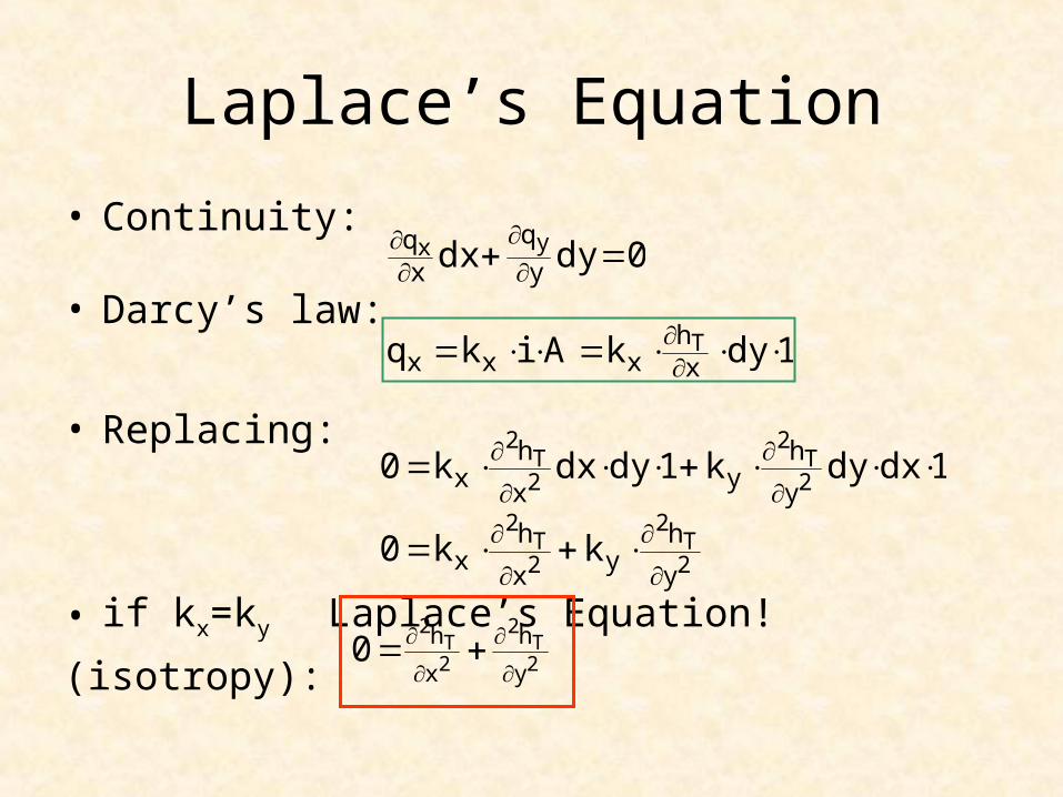
Laplace’s Equation
• Continuity:
• Darcy’s law:
• Replacing:
• if kx=ky Laplace’s Equation!
(isotropy):
0dydx y
q
xq yx
1dykAikq xh
xxxT
1dxdyk1dydxk0 2T
2
2T
2
y
hy
x
hx
2T
2
2T
2
y
hy
x
hx kk0
2T
2
2T
2
y
h
x
h0

Laplace’s Equation
• Typical cases– 1 Dimensional:
linear variation!!
– 2-Dimensional:
– 3-Dimensional:
2T
2
x
h0
ittancons xhT
xbahT
2T
2
2T
2
y
h
x
h0
2T
2
2T
2
2T
2
z
h
y
h
x
h0

Laplace’s Equation Solutions
• Exact solutions (for simple B.C.’s) • Physical models (scaling problems)• Approximate solutions: method of fragments• Graphical solutions: flow nets• Analogies: heat flow and electrical flow• Numerical solutions: finite differences

Flow Nets
• The procedure consists on drawing a set of perpendicular lines: equipotentials and flow lines.
• These set of lines are the solution to the Laplace’s equation.
• It is an iterative (and tedious!) process.• Identify boundaries:– First and last equipotentials– First and last flow lines

Flow Nets
How to draw flow nets
b= l
a

Seepage Calculation from a Flow Net

Seepage Calculation from a Flow Net

Flow Nets
• gradient:
• flow per channel:
• total flow:
Flow channel
Equipotential lines b= l
a
q
h= equipotential drop
bbh
lh
i eNh
Ab
kAlh
kq eNh
e
ff N
Nba
hkNqq

Flow Nets
Number of flow Channels Nf
Number of potential drops Nd

Seepage Calculation from a Flow Net

Seepage Calculation from a Flow Net

Example
Example

16

17

Example - Uplift Pressure
1 2 3 5 64
Point 1: P1 = [(10 + 3) – 0.85]γw = 12.15 γw kN/m2
Potential Drop = H/Nd = (10 – 1.5)/10 = 0.85 m
Point 2: P2 = [(10 + 3) – 2×0.85]γw = 11.3 γw kN/m2
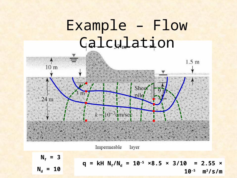
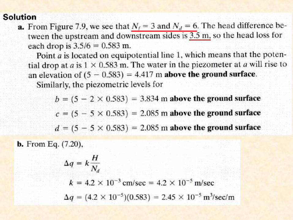
Example – Flow Calculation
Nf = 3
Nd = 10q = kH Nf/Nd = 10-5 ×8.5 × 3/10 = 2.55 × 10⁻⁵ m3/s/m

Uplift Pressure

21

Mathematical Solutions
S/T΄
q/kH
Previous ExampleFlow Net Method
q = 3×2.45×10-5 m3/s/m
Mathematical Method
q = 0.5×4.2×10-5×3.5 m3/s/m
Nf Δq
q = 7.35×10⁻⁵ m3/s/m
q = 7.35×10⁻⁵ m3/s/m
From Figure k H

23

24

25

26

27

28
29


