Using 9C shear wave data to delineate sand in Morrow channels Jasha Cultreri*, Consulting Geophysicist, Allen Gilmer, Vecta Technology, Bob Hardage, University of Texas, Bureau of Economic Geology Summary Incorporating the shear component of multicomponent data has long held the promise of delineating sands from shales. Following the processing methodology outlined by Simmons (SEG 1999), 3D 9C shear wave data is sensitive to the difference in rigidity between sands, shales, and limestones. Two 3D 9 component seismic surveys were acquired to delineate Morrowan drill sites; one in SE Colorado, one in SW Kansas. Two 3D interpretations are presented which show a better than 80% match between 25 wells in eight square miles of 3D 9C seismic data. Twelve to eighteen foot thick sands can be detected. Sands less than six feet thick cannot be detected in these surveys. Shear wave data in both surveys show character anomalies not seen in the P wave data over the sands. An exploratory well was drilled in one of the surveys finding 30% more sand than any of the wells drilled pre-survey. 3D 9C data appears to be very robust in locating and delineating sands incised within a shale sequence. Introduction The Pennsylvanian Morrowan fluvial depositional system across SE Colorado and SW Kansas is similar to many throughout the world. The system is characterized by incised valleys across a broad floodplain. A complex set of fluvial and deltaic sand bodies are deposited in these channels. An excellent modern example of this type of deposition is shown at right in a photograph from southern California. Significant reserves can be found in these sands. Sorrento field alone is estimated to have 29 million barrels oil in place. Total cumulative production in SE Colorado is 94MMBOE. While conventional 2D and 3D compressional wave seismic data is useful in finding some of the incised channels, it has proven to be unsuccessful in locating the sands, especially those incised in shales. Two Surveys Two exploratory 9 component surveys were acquired in this play. Both show detection of Morrowan sands. Standard acquisition parameters are used for both surveys Shear vibrators were used to generate shear inline and shear cross line field data. Standard Compressional vibrators generated the P data. Three component geophones are used to acquire the P, shear inline and shear cross line data. All three geophones are recorded for each source, thus a full nine component data set is recorded which includes all the cross terms – or converted wave data -- see table. S o u r c e s S o u r c e s Receivers Receivers P S X S I P S X S I S X P S X S X S X S I S I P S I S X S I S I Data Processing The primary step (after Simmons 1999 SEG) is rotation to Radial/Transverse coordinate system to extract the Sv and Sh components of the shear wave (Patent BEG/Vecta Technology). Conventional processing of the Sh component data included Decon, Refraction Statics, NMO, Surface Consistent Reflection Statics, Migration, Spectral Whitening, FX Decon, and AGC scaling. Except for velocities about one half of P, and frequencies half of P, the processing is very similar to the P processing. All the shear wave data shown in this case history is Sh component data extracted from the full wave field (9C) data. Case History One – Second Wind Second Wind field is located at the south end of the State Line Morrow fluvial trend. The production bubble map runs N/S along the state line between Colorado and Kansas. At the far southern end of Second Wind field UPRC shot a 3D survey. (Germinario ‘95) In conjunction, a one square mile 9 component survey was acquired. CH 2.4 SEG/Houston 2005 Annual Meeting 440 Main Menu
Transcript
Using 9C shear wave data to delineate sand in Morrow channelsJasha Cultreri*, Consulting Geophysicist, Allen Gilmer, Vecta Technology, Bob Hardage, University of Texas, Bureau of Economic Geology
Summary
Incorporating the shear component of multicomponent data has long held the promise of delineating sands from shales. Following the processing methodology outlined by Simmons (SEG 1999), 3D 9C shear wave data is sensitive to the difference in rigidity between sands, shales, and limestones. Two 3D 9 component seismic surveys were acquired to delineate Morrowan drill sites; one in SE Colorado, one in SW Kansas. Two 3D interpretations are presented which show a better than 80% match between 25 wells in eight square miles of 3D 9C seismic data. Twelve to eighteen foot thick sands can be detected. Sands lessthan six feet thick cannot be detected in these surveys. Shear wave data in both surveys show character anomalies not seen in theP wave data over the sands. An exploratory well was drilled in one of the surveys finding 30% more sand than any of the wells drilled pre-survey. 3D 9C data appears to be very robust in locating and delineating sands incised within a shale sequence.
Introduction
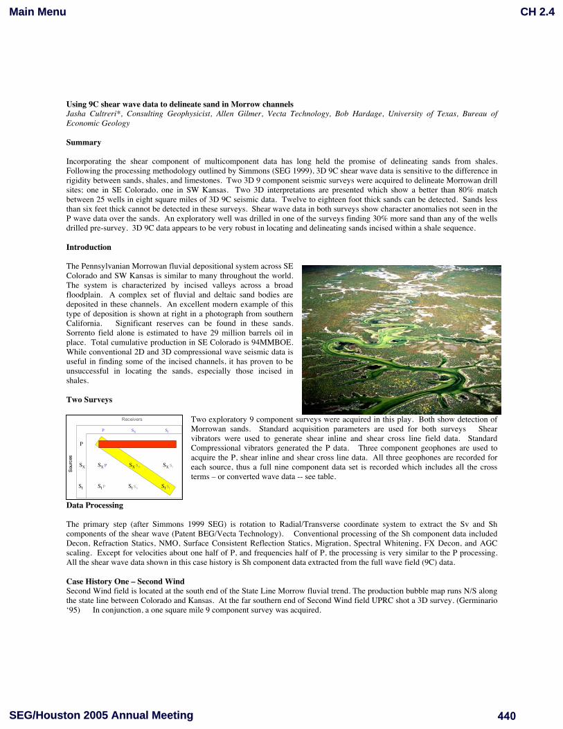
The Pennsylvanian Morrowan fluvial depositional system across SEColorado and SW Kansas is similar to many throughout the world. The system is characterized by incised valleys across a broad floodplain. A complex set of fluvial and deltaic sand bodies aredeposited in these channels. An excellent modern example of this type of deposition is shown at right in a photograph from southern California. Significant reserves can be found in these sands.Sorrento field alone is estimated to have 29 million barrels oil in place. Total cumulative production in SE Colorado is 94MMBOE. While conventional 2D and 3D compressional wave seismic data is useful in finding some of the incised channels, it has proven to be unsuccessful in locating the sands, especially those incised in shales.
Two Surveys
Two exploratory 9 component surveys were acquired in this play. Both show detection of Morrowan sands. Standard acquisition parameters are used for both surveys Shearvibrators were used to generate shear inline and shear cross line field data. StandardCompressional vibrators generated the P data. Three component geophones are used to acquire the P, shear inline and shear cross line data. All three geophones are recorded for each source, thus a full nine component data set is recorded which includes all the cross terms – or converted wave data -- see table.
Sourc
es
Sourc
es
ReceiversReceivers
P SX SI
P
SX
SI
PP P SX P SI
SX P SX SX SX SI
SI P SI SX SI SI
Data Processing
The primary step (after Simmons 1999 SEG) is rotation to Radial/Transverse coordinate system to extract the Sv and Sh components of the shear wave (Patent BEG/Vecta Technology). Conventional processing of the Sh component data included Decon, Refraction Statics, NMO, Surface Consistent Reflection Statics, Migration, Spectral Whitening, FX Decon, and AGC scaling. Except for velocities about one half of P, and frequencies half of P, the processing is very similar to the P processing.All the shear wave data shown in this case history is Sh component data extracted from the full wave field (9C) data.
Case History One – Second WindSecond Wind field is located at the south end of the State Line Morrow fluvial trend. The production bubble map runs N/S along the state line between Colorado and Kansas. At the far southern end of Second Wind field UPRC shot a 3D survey. (Germinario ‘95) In conjunction, a one square mile 9 component survey was acquired.
CH 2.4
SEG/Houston 2005 Annual Meeting 440
Main Menu
9C shear wave / Morrow channels
2 3 71 7 .04 2 65 0 7 .0 0
1 1 4 9. 0
12 2 4 01 9 .0 0
84 6 3 5 .0
48 6 .0 0
5 7 23 9 .09 8 3 .0 0
31 4 4 1 6. 04 0 14 . 00
2 1 9 31 2 .0
78 8 3 .0 0
1 0 4 33 8 .07 0 5 7. 0 0
25 3 4 4. 0
20 1 6 1. 0 0
3 4 3 44 .0
7 0 1 61 .0 0
10 6 .00 .0 0
1 3 93 8 7 .0
6 4 78 . 00
5 33 4 0 .0
6 8 44 5 .0 0
9 7 6 9. 07 48 9 .0 0
87 0 6 8 .054 0 3 8 .0 0
4 5 7 99 . 033 1 6 1 .0 0
1 3 23 3 1 .0
1 9 41 4 .0 023 0 2 7 .0
50 2 0 .0 0
7 6 15 8 .02 0 86 6 .0 0
64 .0
0 .0 0
1 2 35 8 8 .06 6 5 6 8. 00
14 4 2 70 . 07 40 4 8 .0 0
25 4 5 30 . 018 7 8 1. 0 0
36 0 2 7. 0
65 9 0 .0 0
1 4 08 1 3 .02 7 56 6 .0 0
1 0 8 67 5 .02 2 8 63 . 00
13 6 1 52 . 0
5 2 88 2 .0 0
1 4 78 4 9 .05 7 5 3 9. 00
5 4 1 5 5. 05 6 6 0 3. 00
40 5 4 .0
0 .0 0
6 4 39 5 .023 7 8 3. 0 0
12 1 7 66 . 0
4 01 5 6 .0 0
5 7 30 6 .0
32 7 4 3. 0 0
5 14 2 9 .0
1 93 2 7 .0 0
83 8 7 9. 02 6 48 8 .0 0
4 1 24 9 .0
5 5 31 3 .0 0
1 11 4 4 1 .0
5 8 9 88 . 00
4 7 99 6 .03 9 54 1 .0 0
68 6 1 5 .0
2 8 57 1 .0 0
5 4 0 85 . 0
3 7 5 55 . 00
2 9 73 0 .0
6 7 17 8 .0 0
30 7 5 .0
29 8 3 3 .0 0
1 1 95 0 5 .05 7 77 1 .0 0
5 0 41 1 .04 5 38 0 .0 0
6 4 36 . 0
5 2 76 . 00
1 31 0 1 3 .05 6 5 16 . 00
3 04 1 3 .01 0 9 71 .0 0
2 9 14 4 .0
3 3 74 0 .0 0
1 2 3 3 80 .0
4 9 0 5 6. 00
3 6 6 81 .0
5 5 8 81 .0 0
5 74 .03 31 .0 0
5 4 8 95 . 01 9 5 66 7 .0 0
58 7 2 8. 0
5 32 4 1 .0 0
0 . 03 4 3 49 4 .0 0
0. 01 7 84 7 7 .0 0
0 . 0
8 9 5 81 4 .0 0
4 0 3 71 4 4 .0
6 3 9 41 0 6 .0 0
85 4 6 9 7. 045 9 6 9 7. 00
6 85 6 2 .0
4 5 0 15 .0 0
5 20 9 1 .02 60 3 5 .0 0
2 5 6 4 08 .0
4 39 8 8 .0 0
1 3 90 5 4 .0
1 2 27 6 1 .0 0
4 7 9 4. 04 7 1 76 .0 0
3 3 04 2 .027 5 0 3. 0 0
6 1 7 55 . 01 8 9 47 . 00
4 05 1 1 .02 2 3 09 . 00
1 4 1 2 .00 . 00
1 8 6 .025 8 4 1. 0 0
1 3 39 1 .04 2 71 . 00
6 2 6 3 8. 07 35 0 .0 0
1 75 .03 49 .0 0
1 26 6 5 6. 08 43 1 2 .0 0
3 06 3 .0
6 0 15 . 00
2 0 9 2 52 .0
3 5 6 3 1. 00
1 8 17 4 8 .0
19 8 9 71 . 00
7 96 4 1 .03 2 7 50 . 00
90 0 0 0 .01 9 06 . 00
8 18 4 6 .0
6 7 9 68 . 00
2 3 8 6 7. 02 0 8 4 .0 0
3 4 9 3. 0
15 2 7 9. 0 0
16 0 8 8 1. 02 0 91 0 .0 0
1 2 1 44 3 .0
3 3 3 04 . 00
49 6 2 3. 01 2 94 7 .0 0
1 1 6 51 .0
3 8 6 48 .0 0
19 3 4 9 3. 0
94 0 6 5 .0 0
9 0 17 3 .02 0 37 7 .0 0
3 34 9 6 1. 0
3 05 3 6 2. 0 0
9 1 44 2 .06 6 66 .0 0
5 02 3 8 5 .01 4 1 66 8 .0 0
1 1 6 67 . 05 7 1 52 . 00
7 3 4 51 . 03 45 4 0 .0 0
0 .09 2 6 14 5 .0 0
2 2 93 7 0 .0
1 2 00 5 .0 0
81 7 5 2. 0
3 0 95 4 .0 0
18 0 2 7 6. 0
27 6 9 6 5. 00
7 4 7 2. 00 . 00
1 0 1 56 8 .07 8 2 63 .0 0
2 1 4 56 . 04 48 2 8 .0 0
7 3 8 7 5. 0
6 70 6 4 .0 0
1 97 9 8 5. 01 26 8 5 4. 0 0
1 5 14 7 .0
5 0 71 8 .0 0
5 39 8 2 .0
5 74 9 9 .0 0
10 1 8 5 8. 0
24 5 3 9 4. 0 0
6 18 9 9 .0
4 9 9 86 . 00
3 0 6. 04 3 93 2 3 .0 0
65 0 5 2. 034 5 5 8. 0 0
11 5 1 4 3. 0
23 3 2 1 .0 04 16 8 .0
3 53 2 3 .0 0
2 4 4 .04 3 8 38 4 .0 0
19 3 7 8. 0
1 19 0 7 6 .0 0
5 7 19 7
4 8 82 3 .0 0
3 3 1 4 0. 0
7 1 3 9 9. 00
3 7 47 . 0
1 4 65 . 00
8 6 2 26 . 0
4 38 7 3 .0 0
.0
3 1 7
8 8 33 8 .0 0
4 6 6 29 . 0
22 2 2 4 .0 0
41 3 8 1. 071 5 3 8. 0 0
11 3 8 91 . 025 1 2 7. 0 0
2 3 93 1 2 .0
1 9 73 3 3 .0 0
30 3 6 94 . 011 4 3 53 . 00
2 80 1 9 3. 0
2 5 24 6 4 .0 0
18 1 3 00 . 089 9 8 6. 0 0
62 3 4 .0
4 3 61 4 .0 0
62 3 0 .0
10 7 7 4 .0 0
17 1 2 8 1. 0
38 7 1 1 .0 0
7 2 9 0. 061 7 .0 0
0 .03 31 9 4 .0 0
12 3 9 59 . 0
2 5 71 1 .0 0
1 08 1 1 0. 0
4 26 6 9 3. 0 0
5 1 76 6 .0
2 5 9 1 5. 00
5 4 7 90 . 0
1 2 1 45 . 00
4 06 4 2 64 . 0
2 52 8 7 07 . 00
8 9 6 90 . 01 3 0 03 . 00
4 72 1 3 .05 6 8 8. 0 0
1 84 2 8 .0
7 61 0 .0 0
0. 036 5 9 62 . 00
0 . 0
6 7 8 3 .0 0
0 .0
6 3 1 80 . 00
1 7 9 47 . 0
3 9 7 9. 0 0
0 .039 8 7 3 9. 00
8 3 62 2 .01 1 88 8 0 1. 0 0
6 89 0 3 .0
9 87 2 9 4. 0 0
75 3 .0
1 1 23 7 3 7. 0 0
7 60 8 7 83 . 01 8 17 8 2 4 3. 00
1 2 4 60 4 8 .02 1 3 66 0 2 .0 0
52 3 5 5 .0
2 9 57 0 .0 08 9 81 . 00 .0 0
5 6. 01 67 9 6 8. 0 0
1 2 2 .0
0. 0 0
25 0 1 .00 .0 0
4 3 9 1 32 .0 .0 05 2 5 .00 .0 0
2 0 9 9 00 . 00
3 8 5 6 2. 00 . 00
1 7 8 74 9 .00 .0 0
0 .0
4 3 2 .0 00 .0
2 9 7 .0 0
6 5 8 54 5 .0
3 7. 00
2 7 35 5 7 .0
0 .0 0
0 .0
6 2 .0 0
2 36 0 7 3. 00 .0 0
2 4 68 3 0 .00 .0 0
44 9 3 8 .025 0 .0 0
9 7 23 5 .0
1 4 61 7 .0 0
1 8 0 90 7 .00 .0 07 33 4 6 .0
0 .0 06 4 2 9. 0
4 2 3 .0 087 4 4 84 . 0
67 2 9 1. 0 0
45 3 9 9 5. 0
21 8 .0 0
1 6 8 4 8. 0
0 . 00
1 24 8 7 0. 02 4 0 49 . 00
1 0 07 5 .0 . 00
2 9 5 2 9. 00 .0 0
1 54 3 4 3 .0
1 28 0 9 .0 0
3 0 16 5 .00 .0 0
89 2 0 .0
0. 0 0
1 48 7 3 .0
0 .0 0
12 2 3 7. 00. 0 0
1 3 85 .02 1 04 3 4 .0 0
0 .01 82 2 .0 00 . 0
4 8 3 8 .0 0
0 .04 9 52 . 00
1 24 1 9 5. 01 93 2 9 .0 0
1 8 29 4 .01 6 05 .0 0 1 0 5 83 4 .0
0 .0 0
1 32 9 1 .0 .0 0
2 7 18 6 5 .0
0 . 00
1 5 58 7 3 .00 .0 0
2 5 4 80
0 . 00
1 67 1 2 4 .00 .0 0
6 37 7 5 6 .0
0 .0 0
0 .0
6 9 8. 00
0 .0
2 20 7 .0 0
1 00 1 0 .0 .0 0
2 0 14 2 7 .0
0 . 00
9 4 7 3 4. 00 .0 0
3 38 0 5 .0
0 .0 0
7 2 07 8 8 .
0 . 0050 0 7 0 30. 0 0
3 9 1 32 . 00 . 00
4 3 0 8. 00 . 00
1 8 6 90 6 .
0. 0 0
23 7 2 6. 00. 0 0
4 49 0 20 .0 0
3 4 2 29 4 .
0 6 3 .
0
0
5 .0
0
0
. 0
0
0
0 . 004 5 39 2 .0
0 . 00
1 15 9 0 50 .0 0
5 0 6 8. 0 5
0 .0 0
2 7 2 9 7. 00 .0 0
340
1 0 4 44
0. 0 0
21 5 0 27 . 00. 0 0
1 7 20 3 .01 3 1 95 . 00
Second wind survey
10 20 30 40 50 60 70110
20
30
40
50
60
70
80
90
33
0
0
16 0
0
0
20
18
192423
2625
30
313635
2 16
71211
Cox St. 22-26
Cox V
Cox V
Cox V
Higgins FM 11-25
Higgings FM 12-25
Kriss
Kriss
Kriss
Marguerite 44-1
Marion Marion 34-25
Weco Cox St 24-36
Weco Cox St 31-36
Weco Cox St 44-36
Weco-Marguerite 41-1
Sand (VSP well)
Sand
No Sand
No Sand
CHEYENNE CO.
KIOWA CO.LIMITS OF9-C SURVEY
After Germinario
et al 1995
AREA OF FULL FOLD3-D DATA
LIMITS OF V-7 VALLEY
INTERPRETED FROM3-D SURVEY
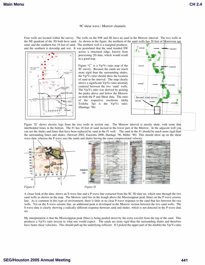
Four wells are located within the survey. The wells on the NW and SE have no sand in the Morrow interval. The two wells in the NE quadrant of the 3D both have sand. As shown in the figure, the northern of the sand wells has 20 feet of Morrowan agesand, and the southern has 18 feet of sand. The northern well is a marginal producer,and the southern is downdip and wet. It was postulated that the sand trended SW
across a structural ridge, known frompreexisting 2D data, which would resultin a good trap.
Figure “C” is a Vp/Vs ratio map of the 9C survey. Because the sands are muchmore rigid than the surrounding shales, the Vp/Vs ratio should show the location of sand in the interval. The map clearlyshows a significant Vp/Vs ratio anomalycentered between the two ‘sand’ wells. The Vp/Vs ratio was derived by picking the peaks above and below the Morrowon both the P and Shear data. The ratio of the respective isochrons (deltaTs/delta Tp) is the Vp/Vs ratio.(Hardage ’96)
Figure ‘D’ shows electric logs from the two wells in section one. The Morrow interval is mostly shale, with some thin interbedded limes in the bottom. The #1 has 18 feet of sand incised in the lower part of the Morrow. In the adjacent well youcan see the shales and limes that have been replaced by sand in the #1 well. The sand in the #1 should be much more rigid thanthe surrounding limes and shales. (Stewart 2002, Gaorotta 2000, Hardage ’96, Miller ‘90) This should show up on the shearwave data, whereas the P wave sees the sands and shales having the same compressional velocity.
Figure C Figure D
A closer look at the data, shows an S-wave line and a P-wave line extracted from the 9C 3D data set, which runs through the twosand wells as shown on the map. The Morrow sand lies in the trough above the Mississippian peak (blue) on the P-wave seismic line. As is common in this type of environment, there is little or no clear P-wave response to the sand that lies between the twowells. Yet on the S-wave seismic line, an additional peak is developed in the Morrow section between the two sand wells. The S-wave data is clearly showing a radically different response between sand and shales, which is not detected in the P-wave dataset.
My interpretation is that the Mississippian peak (blue) is being pushed down by the extra wavelet from the top of the sand. Thisproduces a Vp/Vs ratio inverse to what one would expect. The sands are more rigid than the surrounding shales and therefore have faster shear velocities. This should pull up the underlying reflector. If I picked the upper part of the doublet the Vp/Vs ratio
CH 2.4
SEG/Houston 2005 Annual Meeting 441
Main Menu
9C shear wave / Morrow channels
would be right, but I have no explanationfor the lower peak. Additionally the lower peak looks like a better correlation for the Mississippian. In either case, the Vp/Vsratio anomaly exists only where thedoublet exists, and seems to be associated with the sand in the two flanking wells, one with 20 feet of sand, one with 18.
Case history two – Ashland
A second data set was acquiredacross a Morrow field in Kansas. Ashlandfield has produced approximately700MBOE from 6 wells in an anomalysmaller than 320 acres. Secondaryrecovery efforts are expected to double the recovery. Here again, there is a strong correlation between the S-wave responseand the productive sand wells.
No MorrowSand responsebetween wells?
Sand Response
MorrowMiss
Shear Wave Section (SH)
P Wave Section
Second Wind
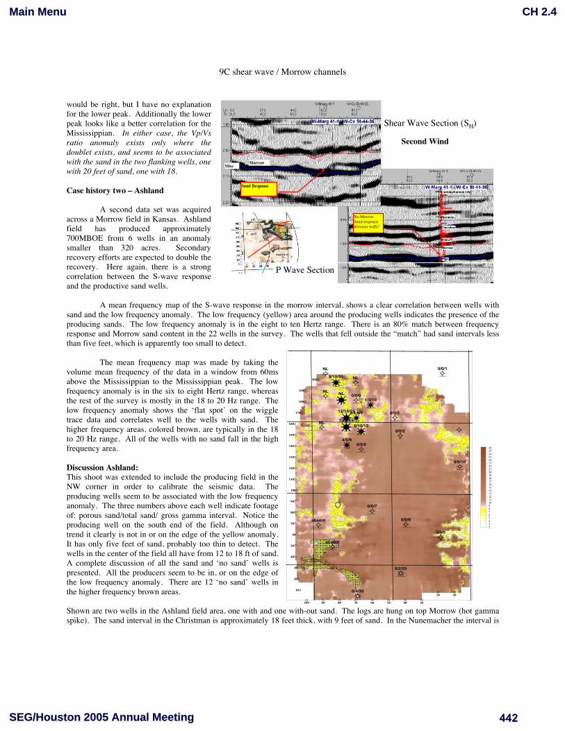
A mean frequency map of the S-wave response in the morrow interval, shows a clear correlation between wells with sand and the low frequency anomaly. The low frequency (yellow) area around the producing wells indicates the presence of the producing sands. The low frequency anomaly is in the eight to ten Hertz range. There is an 80% match between frequencyresponse and Morrow sand content in the 22 wells in the survey. The wells that fell outside the “match” had sand intervals lessthan five feet, which is apparently too small to detect.
10
20
30
40
50
60
70
80
90
100
110
120
130
140
150
160
170
180
190
200
1020
304050607080901001Broadie
1-27Samaniego
1Degnan
1YorkC
1-21Degnan 1-22Edminston
1Broadie
1FinleyA
2-16EulaMay
1-16Judy
1Booth
1-16EulaMay
7
1-16Social Club 1-16Christman
1-9Megan1Gibson1Nunemacher
1Nunemacher
Proinv32-9Megan
2
1-9Robert4Gibson
1 1-10Klinger
Loc
0/4/20
0/2/25
absent
1/4/9
absent 0/0/9
0/0/7
0/0/10
0/0/54/5/9
0/0/26/10/15
NL 7/18/19
4/4.5/712/18/21 0/0/2
1/3/10
NL 0/0/0NL
NL9/12/21
NL 0/0/1
2345678910111213141516171819202122232425262728
The mean frequency map was made by taking the volume mean frequency of the data in a window from 60msabove the Mississippian to the Mississippian peak. The low frequency anomaly is in the six to eight Hertz range, whereas the rest of the survey is mostly in the 18 to 20 Hz range. The low frequency anomaly shows the ‘flat spot’ on the wiggletrace data and correlates well to the wells with sand. The higher frequency areas, colored brown, are typically in the 18to 20 Hz range. All of the wells with no sand fall in the high frequency area.
Discussion Ashland: This shoot was extended to include the producing field in the NW corner in order to calibrate the seismic data. Theproducing wells seem to be associated with the low frequencyanomaly. The three numbers above each well indicate footage of: porous sand/total sand/ gross gamma interval. Notice theproducing well on the south end of the field. Although ontrend it clearly is not in or on the edge of the yellow anomaly.It has only five feet of sand, probably too thin to detect. Thewells in the center of the field all have from 12 to 18 ft of sand.A complete discussion of all the sand and ‘no sand’ wells is presented. All the producers seem to be in, or on the edge ofthe low frequency anomaly. There are 12 ‘no sand’ wells in the higher frequency brown areas.
Shown are two wells in the Ashland field area, one with and one with-out sand. The logs are hung on top Morrow (hot gamma spike). The sand interval in the Christman is approximately 18 feet thick, with 9 feet of sand. In the Nunemacher the interval is
CH 2.4
SEG/Houston 2005 Annual Meeting 442
Main Menu
9C shear wave / Morrow channels
only a couple of feet thick and is all shale. The Vp/Vs ratio of sand is significantly different that shale, and this contrast should show up in the Sh component shear wave data, but not in the P wave
There appears to be a correlation between Valley Fill shale and a Vp/Vs ratio that, in this area,may delineate the ancient valley.
An exploratory well was drilledin the Ashland survey finding 30% more sand than any of the wells drilled pre-survey
ConclusionA greater than 80% fit wasachieved in 26 wells in two 3D 9C surveys. The P data can be effectively used for structuremapping, and after wavefield separation the Sh component shear wave data seems to be quite sensitive to sand in a mostly shale /lime environment. 3D 9C data appears to be very robust in locating and delineating sands incised within a shale sequence.
MRRWSand
MISSLIME
TOPMRRW
ReferencesBrown, , L.G. Miller, W.A., Hundley-Goff, E.M., and Veal, S.L. 1990 Stockholm Southwest Field, Morrow Sandstones of Southeast Colorado and Adjacent Areas, The Rocky Mountain Association of Geologists p 117
Germinario, M.P. Sherrie, R. C. and Suydam, J.R 1995. Applications of 3D Seismic on Morrow Channel Sandstones, SecondWind and Jace Fields, Cheyenne and Kiowa Counties, Colorado, High Definition Seismic Guidebook – Rocky Mountain Association of Geologists p 101-119
Hardage, B.A., 1996 Combining P-wave and S-wave Seismic Data to Improve Prospect Evaluation, Bureau of Economic Geology Report of Investigation No RI 237,
McLeod, D.C. 1986 Sorrento Seen Major SE Colorado Find, Oil and Gas Journal 60-63
Simmons, J. Jr. and Backus, M. 1999 Radial–Transverse (SV-SH) Coordinates for 9-C 3-D Seismic Reflection Data Analysis,Technical Program 69th Annual International Meeting, Society of Exploration Geophysics, (exp. Abs.), V. 1 P 728
Simmons, J. Jr. Backus, M.. Hardage, B. and Graebner, R. 1999 Case History: 3-D Shear–wave Processing and Interpretation inRadial-Transverse (Sv-SH) Coordinates, Technical Program 69th Annual International Meeting, Society of Exploration Geophysics, (exp. Abs.), V. 1 P 792-795
Sonnenburg , S.A., Shannon, L.T. , Rader, K., and VonDrehle, W.F. 1990 Regional Structure and Stratigraphy of the Morrowan Series, Southeast Colorado and Adjacent Areas, Morrow Sandstones of Southeast Colorado and Adjacent Areas, The RockyMountain Association of Geologists, p 1
Sonnenburg, S.A., McKenna, D. and McKenna, P. 1990 The Sorrento Field, Denver Basin, Colorado, Morrow Sandstones of Southeast Colorado and Adjacent Areas, The Rocky Mountain Association of Geologists, p 79
Stewart, 2002 Tutorial Converted Wave Seismic Exploration, SEG Sept 2002 Vol. 67 #5 p 1354
Tathum, R.H. and McCormack M.D. 1991 Multicomponent Seismology in Petroleum Exploration, SEG
Acknowledgements
The authors would like to thank Vecta Exploration and the Bureau of Economic Geology for permission to publish this data.
CH 2.4
SEG/Houston 2005 Annual Meeting 443
Main Menu
EDITED REFERENCES Note: This reference list is a copy-edited version of the reference list submitted by the author. Reference lists for the 2005 SEG Technical Program Expanded Abstracts have been copy edited so that references provided with the online metadata for each paper will achieve a high degree of linking to cited sources that appear on the Web. Using 9C shear wave data to delineate sand in Morrow channels REFERENCES Brown, L. G., W. A. Miller, E. M. Hundley-Goff, and S. L. Veal, 1990, Stockholm
Southwest Field, Morrow Sandstones of Southeast Colorado and Adjacent Areas: The Rocky Mountain Association of Geologists, 117.
Germinario, M.P., R. C. Sherrie, and J. R. Suydam, 1995, Applications of 3D seismic on Morrow Channel Sandstones, Second Wind and Jace Fields, Cheyenne and Kiowa Counties, Colorado: High Definition Seismic Guidebook – Rocky Mountain Association of Geologists, 101-119.
Hardage, B. A., 1996, Combining P-wave and S-wave seismic data to improve prospect evaluation: Bureau of Economic Geology Report of Investigation no. RI 237.
McLeod, D. C., 1986, Sorrento Seen Major SE Colorado Find: Oil and Gas Journal, 60-63.
Simmons, J., Jr., and M. Backus, 1999, Radial–transverse (SV-SH) coordinates for 9-C 3-D seismic reflection data analysis: 69th Annual International Meeting, SEG, Expanded Abstracts, 728.
Simmons, J., Jr., M. Backus, B. Hardage, and R. Graebner, 1999, Case history: 3-D shear–wave processing and interpretation in radial-transverse (Sv-SH) coordinates: 69th Annual International Meeting, SEG, Expanded Abstracts, 792-795.
Sonnenburg, S. A., L. T. Shannon, K. Rader, and W. F. VonDrehle, 1990, Regional structure and stratigraphy of the Morrowan Series, Southeast Colorado and Adjacent Areas, Morrow Sandstones of Southeast Colorado and Adjacent Areas: The Rocky Mountain Association of Geologists, 1.
Sonnenburg, S. A., D. McKenna, and P. McKenna, 1990, The Sorrento Field, Denver Basin, Colorado, Morrow Sandstones of Southeast Colorado and Adjacent Areas: The Rocky Mountain Association of Geologists, 79.
Stewart, R., et al., 2002, Tutorial Converted Wave Seismic Exploration: Geophysics, 67, 1354.
Tathum, R. H., and M. D. McCormack, 1991, Multicomponent seismology in petroleum exploration: SEG.