Segmen tation and Classi cation of Edges Usingtony/papers/cvap186.pdf · for Engineering Sciences,...

Segmentation and Classi�cation of Edges Using

Minimum Description Length Approximation

and Complementary Junction Cues

Tony Lindeberg and Meng-Xiang Li

Computational Vision and Active Perception Laboratory (CVAP)�

Department of Numerical Analysis and Computing Science,KTH (Royal Institute of Technology), S-100 44 Stockholm, Sweden.

Email: [email protected], [email protected]

Technical report ISRN KTH/NA/P{96/01{SE. January 1996.

To appear in Computer Vision and Image Understanding

Abstract

This article presents a method for segmenting and classifying edges using minimumdescription length (MDL) approximation with automatically generated break points. Ascheme is proposed where junction candidates are �rst detected in a multi-scale pre-processing step, which generates junction candidates with associated regions of interest.These junction features are matched to edges based on spatial coincidence. For eachmatched pair, a tentative break point is introduced at the edge point closest to thejunction. Finally, these feature combinations serve as input for an MDL approximationmethod which tests the validity of the break point hypotheses and classi�es the resultingedge segments as either \straight" or \curved". Experiments on real world image datademonstrate the viability of the approach.

Keywords: curve segmentation, minimum description length, corner detection, edge de-tection, curvature, classi�cation, object recognition, computer vision

�We would like to thank G�oran Olofsson for the enjoyable collaboration on the application to objectrecognition as well as for interesting discussions. This work was partially performed under the ESPRIT-BRAproject VAP and the ESPRIT-NSF collaboration Di�usion. The support from the Swedish Research Councilfor Engineering Sciences, TFR, is gratefully acknowledged.

i

ii Lindeberg and Li

Contents

1 Introduction 1

2 Junction Detection with Automatic Scale Selection: Review 2

3 Matching Junctions to Edges 3

4 Minimum Description Length Curve Approximation 3

4.1 Curve Classi�cation by MDL Approximation : : : : : : : : : : : : : : : : 4

4.2 Algorithm : : : : : : : : : : : : : : : : : : : : : : : : : : : : : : : : : : : : 5

5 Experimental results 6

6 Summary and Discussion 15

A Appendix: Algorithmic details 16

A.1 Junction detection, junction localization and edge matching : : : : : : : : 16

A.2 Minimum description length curve approximation : : : : : : : : : : : : : : 17

Edge description using MDL approximation and complementary junction cues 1

1 Introduction

Several object recognition systems for man-made objects are based on detection of imagefeatures, such as edges, in an initial processing step. To reduce the complexity when matchingimage features to a database of object models, an important step in the low-level processing isto derive higher-order descriptors from the image primitives. Concerning edges, one exampleis classi�cation into \straight" or \curved". This step is particularly important within therecognition-by-components paradigm (Binford, 1971; Biederman, 1985; Dickinson et al., 1992;Bergevin and Levine, 1993), where the primitives for object modelling are distinguished bysuch qualitative properties. More generally, the need for classifying edges into \straight"and \curved" arises whenever performing edge based object recognition of curved objects(Requicha, 1980; Fisher, 1989; Grimson, 1990), or when analysing curved objects by line-drawing-like techniques (Malik, 1987).

In its general form, the problem of classifying whether a given edge segment should beregarded as \straight" or \curved" is not well-de�ned. For example, for a given edge seg-ment, the classi�cation may be strongly context dependent. This imposes strong limitationsconcerning the extent to which the results from a low-level classi�cation can be relied upon.Nevertheless, it is in many cases possible to generate reasonable hypotheses. One type ofmethodology that can be used for obtaining such cues is by approximating a given curve us-ing di�erent types of straight and curved models and then selecting the model that accordingto some type of judgement is the one that best �ts the data. Since a more complex model,in general, gives a smaller residual, it is natural to also take the complexity of the modelinto account and aim at a trade-o� between these two factors. This is the idea behind theminimumdescription length (MDL) principle, which focuses on the information contents, andselects the description that can be represented by the smallest number of bits (including themodel as well as the deviations between the model and data).

For elongated edges, which are often obtained from common edge detection methods,it is usually necessary to segment a given curve into smaller patches before attempting aclassi�cation into compact descriptors such as \straight" or \curved". Trying all possibleways of inserting break points into a given (digital) curve obviously leads to combinatorialexplosion. Therefore, it is of interest to develop systematic methods for generating candidatepoints at which the curve is likely to be segmented.

The subject of this article is to show how such candidate break points can be automati-cally generated. The methodology that will be proposed is based on a bottom-up processingstep, where junctions and edges are detected in a complementary manner using multi-scaletechniques. The edges are matched to junctions, and each junction{edge pair constitutes ahypothesis about a point along the edge that is likely to correspond to a corner in the scene.The (elongated) edge segments obtained from the edge detector are then segmented intopatches and each patch is individually classi�ed using a minimum description length curveapproximation method. Finally, adjacent patches are merged if the information contents in acomposed representation is smaller than in the sum of the description lengths of the individualpatches.

The presentation is organized as follows: Section 2 reviews the method for junction de-tection with automatic scale selection on which the overall approach is based. An importantproperty of this method is that each junction candidate is associated with an adaptively de-termined region of interest. This simpli�es the subsequent matching to edges as describedin section 3. Section 4 reviews the speci�c MDL method we use for curve classi�cation anddemonstrates the advantages of using break points as obtained from the proposed approach.Finally, section 5 presents experimental results and section 6 gives a brief summary anddiscussion about the approach.

Concerning overall assumptions, we assume that the underlying image data have beenacquired from scenes of man-made objects that can be well described by object models ofgeon-type and for which a classi�cation into the given set of qualitative descriptors (straightand curved) is su�cient.

2 Lindeberg and Li

2 Junction Detection with Automatic Scale Selection: Review

The fact that image structures exist as meaningful entities only over certain ranges of scaleshows that a multi-scale approach is essential when extracting information, such as features,from image data. Whereas scale-space theory (Witkin, 1983; Koenderink, 1984) provides acanonical framework for modelling visual operations at multiple scales, it is in many casesnecessary to complement this framework by explicit mechanisms for generating hypothesesabout appropriate scales (Lindeberg, 1994c).

A junction detector with automatic scale selection has been developed by Lindeberg (1993c,1994a). It is beyond the scope of this article to extensively describe this method or to mo-tivative the need for a scale selection mechanism with respect to the problem of junctiondetection. Since, however, a number of the speci�c properties of this method are importantfor the proposed methodology, we shall brie y review its most important steps:

The scale-space representation L : R2 � R! R of a two-dimensional signal f : R2 ! R

is de�ned as the one-parameter family of functions obtained by convolving f with Gaussiankernels g : R2�R! R of di�erent widths,

L(�; t) = g(�; t) � f (1)

where t is the scale parameter of the Gaussian g(x1; x2; t) = 1=(2�t) e�(x21+x2

2)=2t. In this

representation, normalized derivatives are de�ned by

@� =pt @x: (2)

Over the years, a large number of di�erent approaches to corner detection have been devel-oped, see for example (Kitchen and Rosenfeld, 1982; Dreschler and Nagel, 1982; Koenderinkand Richards, 1988; Noble, 1988; Deriche and Giraudon, 1990; Blom, 1992; Florack et al.,1992; Rohr, 1992). To detect junction candidates from grey-level images, we shall in this ar-ticle follow the commonly used di�erential approach of de�ning a junction detector in termsof the curvature of level curves multiplied by the gradient magnitude raised to some power.Selecting the power of three gives

~� = L2x2Lx1x1 � 2Lx1Lx2Lx1x2 + L2

x1Lx2x2 : (3)

known as the rescaled level curve curvature. Then, replacing each derivative by its corre-sponding normalized derivative gives normalized rescaled level curve curvature

~�norm = t2~�: (4)

The method in (Lindeberg, 1993c, 1994a) is based on the detection of scale-space extrema(simultaneous maxima over scale and space) of ~�2norm. In addition to allowing for featuredetection without external choice of scale levels, an attractive property of this approach isthat the selected scale levels at which the maxima over scales are assumed, will be largerfor corners that have a large spatial extent in the image domain. In other words, the scale-space maxima serve as indicators re ecting of the spatial extent of the corresponding imagestructures.

Figure 1(b) shows the 100 most signi�cant junction candidates extracted from an image ofan o�ce scene. Each scale-space maximum is illustrated by a circle with the area proportionalto the scale at which the maximum is assumed. Note that coarser scales are selected for thejunctions having larger spatial extent and vice versa.

In the abovementioned references, it has been argued that such qualitative scale andregion descriptors are useful for guiding later processes stages. Here, we shall use this typeof attribute information for de�ning an adaptively determined region of interest around eachjunction candidate, which will be used when matching junctions to edges. More generally, suchregional descriptors can also be used for purposes such as junction classi�cation (Brunnstr�omet al., 1992) and junction tracking (Bretzner and Lindeberg, 1995).

Whereas the junction detection step is conceptually clean, it can certainly lead to poorlocalization. One way to improve the localization is by applying a modi�ed F�orstner operator


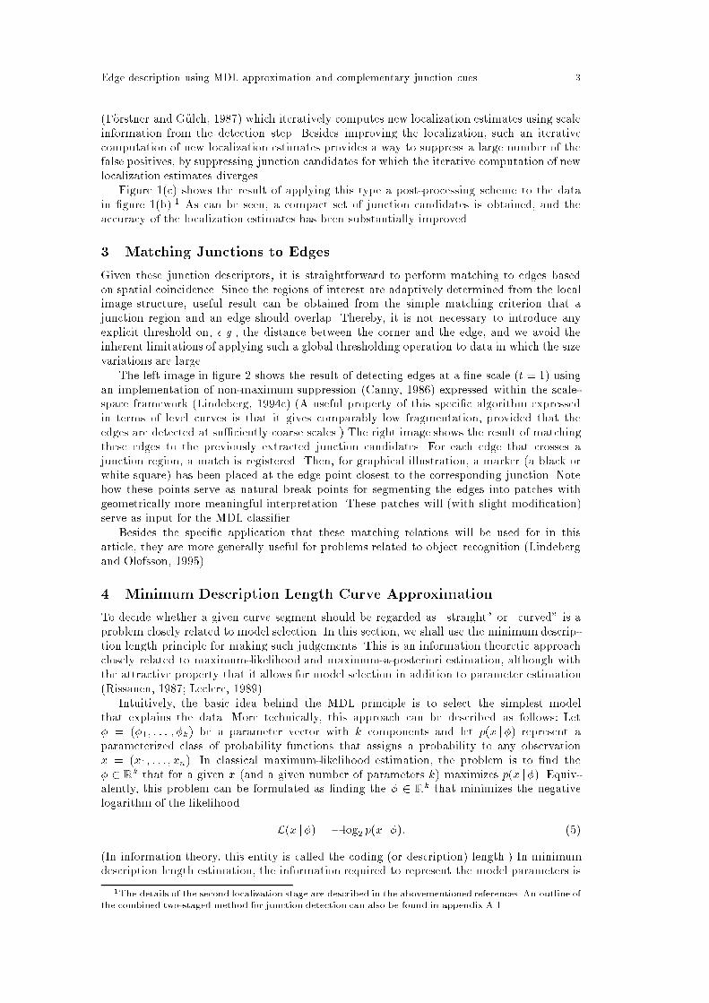
(F�orstner and G�ulch, 1987) which iteratively computes new localization estimates using scaleinformation from the detection step. Besides improving the localization, such an iterativecomputation of new localization estimates provides a way to suppress a large number of thefalse positives, by suppressing junction candidates for which the iterative computation of newlocalization estimates diverges.

Figure 1(c) shows the result of applying this type a post-processing scheme to the datain �gure 1(b).1 As can be seen, a compact set of junction candidates is obtained, and theaccuracy of the localization estimates has been substantially improved.

3 Matching Junctions to Edges

Given these junction descriptors, it is straightforward to perform matching to edges basedon spatial coincidence. Since the regions of interest are adaptively determined from the localimage structure, useful result can be obtained from the simple matching criterion that ajunction region and an edge should overlap. Thereby, it is not necessary to introduce anyexplicit threshold on, e.g., the distance between the corner and the edge, and we avoid theinherent limitations of applying such a global thresholding operation to data in which the sizevariations are large.

The left image in �gure 2 shows the result of detecting edges at a �ne scale (t = 1) usingan implementation of non-maximum suppression (Canny, 1986) expressed within the scale-space framework (Lindeberg, 1994c) (A useful property of this speci�c algorithm expressedin terms of level curves is that it gives comparably low fragmentation, provided that theedges are detected at su�ciently coarse scales.) The right image shows the result of matchingthese edges to the previously extracted junction candidates. For each edge that crosses ajunction region, a match is registered. Then, for graphical illustration, a marker (a black orwhite square) has been placed at the edge point closest to the corresponding junction. Notehow these points serve as natural break points for segmenting the edges into patches withgeometrically more meaningful interpretation. These patches will (with slight modi�cation)serve as input for the MDL classi�er.

Besides the speci�c application that these matching relations will be used for in thisarticle, they are more generally useful for problems related to object recognition (Lindebergand Olofsson, 1995).

4 Minimum Description Length Curve Approximation

To decide whether a given curve segment should be regarded as \straight" or \curved" is aproblem closely related to model selection. In this section, we shall use the minimumdescrip-tion length principle for making such judgements. This is an information theoretic approachclosely related to maximum-likelihood and maximum-a-posteriori estimation, although withthe attractive property that it allows for model selection in addition to parameter estimation(Rissanen, 1987; Leclerc, 1989).

Intuitively, the basic idea behind the MDL principle is to select the simplest modelthat explains the data. More technically, this approach can be described as follows: Let� = (�1; : : : ; �k) be a parameter vector with k components and let p(x j�) represent aparameterized class of probability functions that assigns a probability to any observationx = (x1; : : : ; xn). In classical maximum-likelihood estimation, the problem is to �nd the� 2 Rk that for a given x (and a given number of parameters k) maximizes p(x j�). Equiv-alently, this problem can be formulated as �nding the � 2 Rk that minimizes the negativelogarithm of the likelihood

L(x j�) = � log2 p(x j�): (5)

(In information theory, this entity is called the coding (or description) length.) In minimumdescription length estimation, the information required to represent the model parameters is

1The details of the second localization stage are described in the abovementioned references. An outline ofthe combined two-staged method for junction detection can also be found in appendix A.1.

4 Lindeberg and Li

taken into account as well, leading to minimization of

L0(x; �) = L(x j�) + L(�) = � log2 p(x j�) + L(�): (6)

where L(�) is a measure of the information contents in the parameters.

4.1 Curve Classi�cation by Minimum Description Length Approximation

In computer vision, the MDL approach has been applied to several problems; see for example(George� and Wallace, 1985; Darell et al., 1990; Deren et al., 1990; Axelsson, 1992; Shein-vald et al., 1992). Here, we shall consider the scheme for MDL-based curve approximationdeveloped by (Li, 1993) (which will be extended in several ways). It concerns the problem ofrepresenting a digital curve using the following models:

� a set of randomly distributed points,

� a linear model with or without outliers,

� a segment of an ellipse with or without outliers.

Given these shape classes, any edge segment is classi�ed as \straight" if the linear model givesthe shortest description and as \curved" if the ellipse approximation results in the shortestone. For each model, the description length is measured by

L0(x; �) = (L# points + Lparameters+ Lmodel points + Loutliers)(x; �) (7)

where

� L# points(x; �) is the number of bits needed to represent the total number of points.(This term is similar for all models and not relevant for comparisons.)

� Lparameters(x; �) is the description length of the model parameters.

� Lmodel points(x; �) is the description length for the (N � �) points that belong to themodel.

� Loutliers(x; �) speci�es the description length of � points classi�ed as outliers.

An essential parameter when measuring the description length in a minimum descriptionlength approximation method is the spatial resolution " at which the approximation is per-formed. Assuming that a variable x is uniformly distributed in some interval [x0; x0 + �x]of width �x, the description length of this variable approximated to resolution � can bemeasured by

Lcoord(�x; ") = log2�x

": (8)

When x represents a coordinate of an image point, �x does of course correspond to the imagesize. Concerning the choice of ", it is natural to set this parameter to a value of the same orderas the distance between adjacent pixels. (Here, for edges detected with subpixel resolution atscale t = 1:0, we have used " = 0:5.)

Then, based on this construction, and assuming an image of size M � M pixels, thedescription lengths of the di�erent terms in (7) can be measured as follows:

� Model parameters: To parameterize a straight line segment, four parameters are needed.We can, for example, take the four coordinates determining its end points, which gives

Lline-segment(x; �) = 4Lcoord(N ; ") = 4 log2M

": (9)

The same idea can be applied to the ellipse segment model, which can be described byseven parameters. The center of the ellipse (xc; yc) and the lengths of the two semi-axesa and b can be modelled by uniformly distributed coordinates in the image resulting


in a description length of the same form as in (9). Then, we can add three angulardescriptors describing the orientation of the ellipse as well as the two end points of theellipse segment. Since the ellipse size will, in general, be much smaller than the imagesize, we can parameterize these descriptors by their projections on the coordinate axesquantized relative to the spatial extent of the ellipse. If we model the size of the ellipseby 2max(a; b), the total description length of the ellipse segment will then be of theform

Lellipse-segment(x; �) = 4Lcoord(N ; ") + 3Lcoord(2max(a; b); ")

= 4 log2M

"+ 3 log2

2max(a; b)

"(10)

� Model points: To capture approximation errors, the description length of the (N � �)model points is measured by

Lmodel points(x; �) = (N � �)Lo�set(�;�): (11)

where Lo�set(�;�) is the coding length of the o�set error, i.e., the amount of informa-tion required for representing the distance between a data point and the closest pointbelonging to the model.

Here, the latter entity is approximated by the expected coding length of the outcomeof a centered Gaussian distribution � � N (0; �2) quantized with resolution ". With

�(�; �2) =R ��=�1

g(�; �2) d�, and [�]" denoting the integer multiple of " closest to �,we have

Lo�set(�;�) = � log2

Z [x]"�"=2

�=[x]"+"=2

g(�; �2) d�

!(12)

= � log2��([�]" +

"2 ; �

2)� �([�]" � "2 ; �

2)�

� log2�g(�; �2) "

�=

log2 e

2

�2

�2+ log2

��"

�+log2(2�)

2; (13)

where � represents the primitive function of the Gaussian kernel and � is estimatedfrom the actual deviations between the model and the data (see also F�orstner (1989)).

� Outliers: The � points classi�ed as outliers are modelled as random points having auniform distribution in the image domain. Hence, the total description length of the �points classi�ed as outliers is measured by

Lrandom point = 2�Lcoord(N ; ") = 2� log2M

": (14)

4.2 Algorithm

Given edges and junctions detected as outlined in section 2 with candidate break pointsgenerated from the junction-edge matching in section 3, this data is used as input for theMDL approximation scheme.

The edge points from the junction-edge matches serve as tentative break points for splittingedge segments into shorter ones. Moreover, co-linear and co-curvilinear edge segments (whoseend points are adjacent) are candidates for being merged. Depending on which model gives theshortest description, segments are merged (cases (a){(b)) and split (cases (c){(e)) as shownin �gure 3. To allow for merging of fragmented edges, small gaps are �lled in if a composedmodel gives a more compact description.

Another useful processing step is to move the break point along the curve and select theposition that minimizes the total description length (see �gure 4). Whereas the validity ofeach break point is evaluated in this algorithm and a better position estimate is computedas well, the major advantage of the proposed approach is that a conservative set of junctioncandidates is obtained. Restricting the processing to these points serves as a heuristic principlefor reducing the otherwise combinatorial explosion in guessing where to split elongated edgesegments into shorter ones.2

2An obvious alternativewould be to determine such candidate break points based on edge informationonly,

6 Lindeberg and Li

5 Experimental results

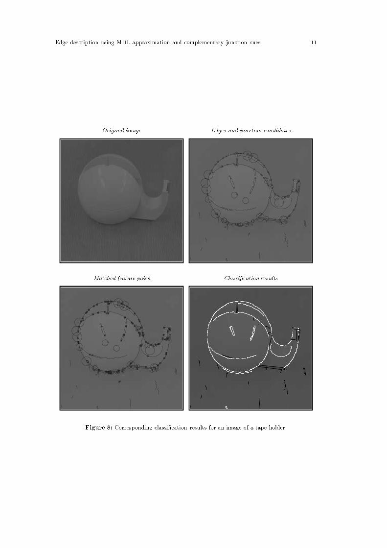
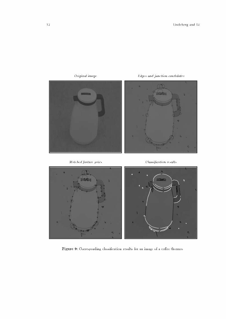
Figure 5 shows the �nal result of applying the composed procedure3 to the image in �gure 1using the image features and candidate break points shown in �gure 2. For graphical illus-tration, straight edge segments have been marked by black lines and curved ones by white.(In the graphical illustration of the classi�cation, all points classi�ed as outliers have beensuppressed, which results in a loss of connectivity at some junctions. Internally, however, thecomplete representations can be maintained.) Figures 6{11 show corresponding results fora set of images of other geon-type objects. Notice how very reasonable segmentations andclassi�cations are obtained.

e.g. by detecting points where the curvature of the edge is high. Computing the edge curvature, however, leadsto a scale problem, concerning the scale at which to de�ne descriptors such as curvature extrema. Whereaswe do not argue that such purely edge based approaches should not be used, we argue that the potential incomputing breakpoint descriptors directly from the grey-level information should be higher. One major reasonfor this is that a corner detector operating directly on the image data has access to much more information(the entire grey-level pattern). Another as important reason, and as will be further emphasized in section 6,is that in applications such as object detection, explicit computation of junction candidates from grey-levelpatterns will nevertheless be highly useful, as will the matching relations be between edges and junctions.(More generally, one could, of course, consider hybrid methods, in which these two approaches are combined.Such a method would obviously be bene�cial in situations when either of the approaches fails as a single cue.)

3A detailed description of the algorithmic steps involved is given in appendix A.2.


Figure 1: (left) An o�ce scene with geon-type objects. (middle) Junction candidates detected byselecting the 100 scale-space maxima having the strongest (maximal) normalized response. (right)Improved localization estimates obtained by applying a modi�ed F�orstner operator to each junctioncandidate. (From (Lindeberg, 1994a).)

Figure 2: (left) Edges detected by non-maximum suppression with junction candidates overlayed.(right) Matched edge-junction pairs illustrated by squares centered at the edge point closest to thecorresponding junction.

S

S

1

2

p S

S

1

2

pS

S

1

2

p S S1 2p S

S

1

2

p

(a) (b) (c) (d) (e)

Figure 3: Five examples of splitting or merging of edge segments. (a) S1 and S2 are co-linear andbelong to the same segment. (b) S1 and S2 co-curvilinear and belong to the same curved segment.(c) S1 and S2 are two non-collinear straight segments and P is a corner point. (d) S1 and S2 are twocurved segments that are not co-curvilinear. Most likely, P is an in exion point. (e) S1 is straight,S2 is curved and P is a transition point from straight to curved.

8 Lindeberg and Li

-5 0 5 10 15 20

p1

p2

p1

p2

Figure 4: Adjustment of break points. The left �gure shows input segments with initial candidatebreak points illustrated by small circles and new positions marked by larger circles. The new positionis obtained by moving the break point along the curve and selecting the break point that minimizesthe total description length. The curves in the right �gure show how the total description lengthvaries as the break point is moved along the curve.

Figure 5: Classi�cation results for the image in �gure 1(a) using the image features and candidatebreak points from �gure 2(b). Straight edge segments are marked by black and curved ones by white.Dark curves indicate edges which are regarded as unclassi�ed, i.e. edges for which the descriptionlengths for the straight and curved edge models are almost the same (here, di�er less than 5 %).


Original image Edges and junction candidates

Matched feature pairs Classi�cation results

Figure 6: Results of edge classi�cation for a scene with wooden blocks. The images show fromtop left to bottom right; (a) the original image, (b) edges and junctions detected as described insection 2, (c) break points obtained according to the scheme in section 3, and (d) the �nal resultof the classi�cation. In the last image, the straight edges have been marked by dark lines and thecurved edges by bright curves. (Edge segments for which the description lengths for the straight andcurved edge models are almost the same (di�er less than 5 %) are illustrated as black curves.)

10 Lindeberg and Li



Figure 7: Corresponding classi�cation results for a scene with textured wooden blocks.




Figure 8: Corresponding classi�cation results for an image of a tape holder.

12 Lindeberg and Li



Figure 9: Corresponding classi�cation results for an image of a co�ee thermos.




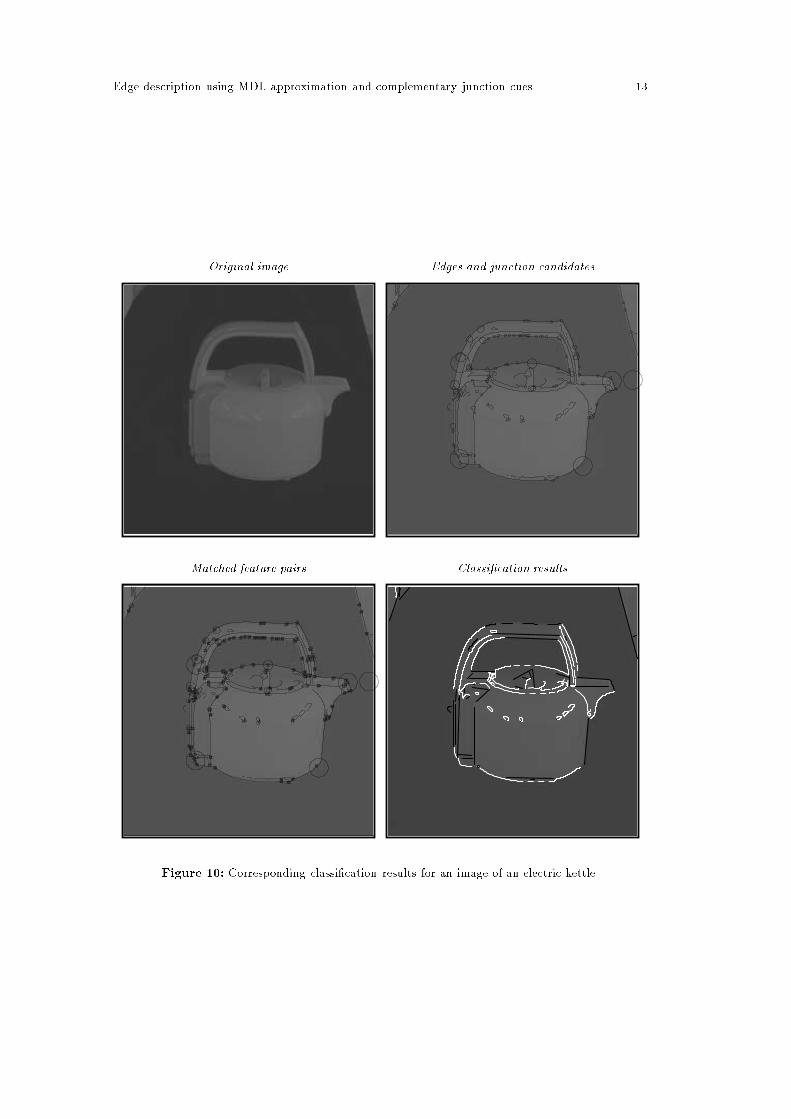
Figure 10: Corresponding classi�cation results for an image of an electric kettle.

14 Lindeberg and Li



Figure 11: Corresponding classi�cation results for an image of a telephone and a calculator.


6 Summary and Discussion

We have shown how break points for MDL classi�cation can be generated in a straightforwardmanner by combining edge data with a speci�c type of junction descriptor associated with anatural region of interest. Instead of operating on the curves as isolated objects and trying to�nd break points based on, e.g., di�erential properties such as curvature extrema, these pointsare obtained by a complementary technique based on junction cues computed directly from thegrey-level information. When integrated with edge cues, these junction cues not only reducethe (combinatorial) computational complexity in the algorithm for computing the minimumdescription length approximation; they also provide important object features for making thesegmentation and classi�cation results more robust to noise and outliers. Experimentally, thisapproach has been demonstrated to give highly useful results on real-world data, especiallyconsidering the fact that this low-level processing operates without any access to higher-levelinformation.

Concerning limitations of the work, it has throughout been assumed that the image dataoriginate from man-made objects and that the simple shape classes \straight line", \ellipsesegment", and \random points" are su�cient for modelling the data and providing reasonablemeasures of the description length. For more complex natural scenes, extensions are required,in particular concerning the choice of primitives for measuring the description length.

Another limitation is due to the inherent di�culty in making a �nal decision between\straight" and \curved" at a low level. (For example, the intuitive judgement of whether agiven segment should be regarded as \straight" or \curved" may vary depending on whatadditional information is available.) When using these data as input to an object recognitionsystem, it is therefore more natural to associate a con�dence measure with each featureclassi�cation (e.g. the ratio between the shortest and the next shortest description length)to allow for �nal decisions to be made at higher processing levels where more information isavailable.

Underlying philosophies of the approach. Let us �nally remark that whereas this article hasbeen mainly concerned with the rather speci�c problem of classifying edges as \straight" or\curved" using minimum description length approximation as the decision rule, the main in-tention has not been to propose speci�c algorithms, but to illustrate computational principles.There are a number of general ideas underlying this approach, which we argue should be ofmuch wider applicability:

(i) By making complementary use of edges and corners, we have access to a much richersource of information than if basing the analysis on edge cues only. For example, the relationsbetween edge and corner descriptors, possibly combined with associated feature classi�cations,will be highly useful for problems such as object recognition.

(ii) By using a bottom-up multi-scale preprocessing step to select interesting scale levels,rank image structures on saliency and delimit regions of interest, we can simplify the tasksfor further/re�ned processing. Such local context information can serve as a heuristic guidefor reducing the search space for reasoning algorithms and for reducing the combinatorialcomplexity in evaluating decision criteria, such as those based on the minimum descriptionlength paradigm.

16 Lindeberg and Li

A Appendix: Algorithmic details

This section gives a more in-depth description of the major implementation issues.

A.1 Preprocessing: Junction detection, junction localization and edge matching

The combined method for junction detection, junction localization and edge matching in sections 2-3is based upon the following algorithmic steps (Lindeberg, 1994a, 1994b):

1. Detection: Given a discrete image f (here: of size 128� 128 or 256� 256 pixels), select a scalerange for the analysis (here: tmin = 4 and tmax = 256). Within this range, distribute a set ofscale levels tk (here: 20 or 40 levels) such that the ratio between successive scale levels tk+1=tkis approximately constant. (You can choose these levels such that the di�erence in e�ectivescale (Lindeberg, 1993b) �k+1 � �k is constant.)

2. For each tk, compute the scale-space representation of f by convolution with the discreteanalogue of the Gaussian kernel T (Lindeberg, 1994c): L(�; tk) = T (�; tk) � f .

3. For each point at each scale, compute discrete derivative approximations of L(�; tk) by centraldi�erences (Lindeberg, 1993a) and multiply the �rst- and second-order di�erences by

ptk and

tk, respectively. (More accurately, you can determine a discrete normalization factor such thatthe l1 norm of the corresponding discrete derivative approximation kernel is constant overscales (Lindeberg, 1994c).) Combine these normalized derivatives into discrete approximationsto ~�2norm at each point using (3).

4. Finally, in the three-dimensional volume generated, detect local maxima (as points whose valuesare greater than or equal to the values of their 26 discrete neighbours) and select the N (here:100 or 400) points having the strongest normalized response.

5. Localization: For each junction candidate detected in this way, determine an improved local-ization estimate by computing the following weighted integrals

A =

Z(rL) (rL)T dx0; b =

Z(rL) (rL)T x0 dx0; c =

Zx0

T(rL) (rL)T x0 dx0:

using a Gaussian window function with (integration) scale value equal to the detection scaleand with the center at the candidate junction. At a number of scales (here: 10 levels), uniformlydistributed between a lower scale (here: 0.01) and the detection scale, vary the (local) scaleat which derivatives are computed and select the (local) scale that minimizes the normalizedresidual over scales

~dmin = mint2[0;tdet]

minx2R2

xTAx� 2xT b+ c

traceA= min

t2[0;tdet]

c� bTA�1b

traceA: (15)

6. At this scale, the new localization estimate is x̂ = A�1b.

7. Iterate the localization steps (5{7) until either the increment is su�ciently small (here: withinthe same pixel) or an upper bound (here: 3 iterations) has been reached. Suppress all pointsfor which the scheme diverges (here: when the total update is larger than the detection scalemeasured in dimension [length]).

8. Edge detection. Concerning the edge detection step, we have throughout this work assumedthat edges are given as input. For the experiments presented in this article, edges have beendetected at a �xed scale (tedge = 1:0), using hysteresis thresholding on the gradient magnitude.Unless otherwise stated, the low and high thresholds (jrLj > 4:0 and jrLj > 8:0) have beenthe same for all images.

Whereas substantial improvements could be obtained by integrating the evaluation of edgeswith other processing modules, and by including explicit mechanisms for scale selection (Lin-deberg, 1995) with locally adapted thresholding operations, we have no aim of contributing tothe problem of edge detection in this article.

9. Edge matching. Represent each remaining junction candidate with a circle with area equal tothe detection scale tdet. For each (connected) edge that intersects such a circle, register an edgematch at the edge point closest to the localized junction.

When implementing this method in practice, the following observations improve the computationale�ciency: On a serial computer, it is not necessary to pre-compute ~�2norm at all scales before detectingscale-space maxima; it is su�cient to keep three images in the memory. To reduce the combinatorics


in the junction-edge matching, the junctions can be stored in an image-like representation to avoidexhaustive search in a list of junction candidates.

To reduce the computational work further, it can in many situations be su�cient to use morenarrow scale ranges than indicated here (e.g. tmax = 20), a smaller number of scale levels (e.g. 7 or10 scales in the detection stage and 2 or 3 levels in the localization stage), and to perform justone iteration in the iterative re�nement. The computational e�ciency of this processing step is alsoimproved substantially by reducing the spatial sampling density (subsampling the data) at coarserscales in scale-space.

A.2 Minimum description length curve approximation

The input to this curve approximation algorithm is a set of edge segments (represented as lists ofpoints) and a set of candidate break points at which the edge segments may be split into parts. Foreach edge segment, the algorithm approximates the curve by a straight and a curved model accordingto section 4.1, considers possible ways of merging edge segments, and outputs a judgement of whetherthe segment should be regarded as straight or curved. In summary, for each candidate break point,the following operations are performed:

1. Segment de�nition. Include edge points from the current point in the forward and backwarddirections along the edge segment until either another break point has been reached or an endpoint is encountered. Denote these two curves by S1 and S2.

2. Local models. Compute the description lengths for the following models of S1 and S2:

Mll : S1 and S2 are collinear, so S1 and S2 belong to the same segment,

M_cc : S1 and S2 co-curvilinear, e.g., they belong to a piece of elliptical segment,

Mbll: S1 and S2 are two straight segments but not collinear,

Mcc : S1 and S2 are two curved segments but they are not co-curvilinear,

Mlc : S1 is straight and S2 is curved,

Mcl : S1 is curved and S2 is straight,

In this step, straight line and ellipse models are �rst �tted to S1, S2 and the concatenationof S1 and S2 using standard approximation techniques. Then, outliers are removed iterativelyin a local greedy fashion, by identifying the point with the highest residual, re-doing the �twithout this point, and repeating this removal until the description length does not decrease.

3. Model selection and merging. Choose the approximation model with the minimum descriptionlength. If the minimum is assumed for Mll or M_cc , then merge these edge segments and go tothe next break point (step 1). Otherwise, continue with step 4.

4. Break point re�nement.Move the candidate break point in the forward and backward directionswhile evaluating the composed approximation models in step 2. Then, split the edge segmentat the position at which the minimum description length is assumed.

Finally, allow small edge gaps to be closed and classify the results as follows:

5 Merging and gap closing.For each pair of edge segments whose end points are su�ciently close,evaluate the models according to step 2. Merge the segments if the minimum is assumed forMll or M_cc . Otherwise, keep them separate.

6 Classi�cation. For each new curve, compute the description lengths for the linear and ellipticapproximation models. Classify the segment as straight if the minimum is assumed for thelinear model and as curved if it is assumed for the elliptic one.

18 Lindeberg and Li

References

Axelsson, P. (1992). Minimum description length as an estimator with robust properties. InW. F�orstner et al., editor, Proc. of International Workshop on Robust Computer Vision, pp. 137{150.

Bergevin, R. and Levine, M. D. (1993). Generic object recognition: Building and matching coarsedescriptions from line drawings. IEEE Trans. Pattern Analysis and Machine Intell., 15, no. 1,19{36.

Biederman, I. (1985). Human image understanding: Recent research and a theory. In Human and

Machine Vision II, pp. 13{57. Academic Press.Binford, T. O. (1971). Visual perception by computer. In IEEE Conference on Systems and Control,

Miami, Florida.Blom, J. (1992). Topological and Geometrical Aspects of Image Structure. PhD thesis, Dept. Med.

Phys. Physics, Univ. Utrecht, NL-3508 Utrecht, Netherlands.Bretzner, L. and Lindeberg, T. (1995). Feature tracking with automatic selection of spatial scales.

(Submitted).Brunnstr�om, K., Lindeberg, T., and Eklundh, J.-O. (1992). Active detection and classi�cation of

junctions by foveation with a head-eye system guided by the scale-space primal sketch. In San-dini, G., editor, Proc. 2nd European Conf. on Computer Vision, volume 588 of Lecture Notes inComputer Science, pp. 701{709, Santa Margherita Ligure, Italy. Springer-Verlag.

Canny, J. (1986). A computational approach to edge detection. IEEE Trans. Pattern Analysis and

Machine Intell., 8, no. 6, 679{698.Darell, T., Sclaro�, S., and Pentland, A. (1990). Segmentation by minimum description. In Interna-

tional Conference on Computer Vision, pp. 112{116, Osaka, Japan.Deren, D., Marcus, R., Werman, M., and Peleg, S. (1990). Segmentation by minimum length encoding.

In Proc. 10th Int. Conf. on Pattern Recognition, pp. 681{683, Atlantic City, N. J.Deriche, R. and Giraudon, G. (1990). Accurate corner detection: An analytical study. In Proc. 3rd

Int. Conf. on Computer Vision, pp. 66{70, Osaka, Japan.Dickinson, S. J., Pentland, A. P., and Rosenfeld, A. (1992). From volumes to views: An approach to

3-D object recognition. CVGIP: Image Understanding, 55, no. 2, 130{154.Dreschler, L. and Nagel, H.-H. (1982). Volumetric model and 3D-trajectory of a moving car derived

from monocular TV-frame sequences of a street scene. Computer Vision, Graphics, and Image

Processing, 20, no. 3, 199{228.Fisher, R. B. (1989). From Surfaces to Objects. John Wiley and Sons, Chichester, England.Florack, L. M. J., ter Haar Romeny, B. M., Koenderink, J. J., and Viergever, M. A. (1992). Scale

and the di�erential structure of images. Image and Vision Computing, 10, no. 6, 376{388.F�orstner, M. A. and G�ulch, E. (1987). A fast operator for detection and precise location of distinct

points, corners and centers of circular features. In Proc. Intercommission Workshop of the Int.

Soc. for Photogrammetry and Remote Sensing, Interlaken, Switzerland.F�orstner, W. (1989). Image analysis techniques for digital photogrammetry segmentation by mini-

mum description. In Proceedings of the 42'nd Photogrammetric Week, Stuttgart.George�, M. P. and Wallace, C. S. (1985). A general selection criterion for inductive inference. In

O'Shea, T., editor, Advances in Arti�cial Intelligence, pp. 219{229.Grimson, W. E. L. (1990). Object Recognition by Computer: The role of geometric constraints. MIT

Press, Cambridge, Massachusetts.Kitchen, L. and Rosenfeld, A. (1982). Gray-level corner detection. Pattern Recognition Letters, 1,

no. 2, 95{102.Koenderink, J. J. (1984). The structure of images. Biological Cybernetics, 50, 363{370.Koenderink, J. J. and Richards, W. (1988). Two-dimensional curvature operators. J. of the Optical

Society of America, 5:7, 1136{1141.Leclerc, Y. G. (1989). Constructing simple stable descriptions for image partitioning. Int. J. of

Computer Vision, 3, 73{102.Li, M. (1993). Minimum description length based 2-D shape description. In et. al., H.-H. Nagel,

editor, Proc. 4th Int. Conf. on Computer Vision, pp. 512{517, Berlin, Germany. IEEE ComputerSociety Press.

Lindeberg, T. (1993a). Discrete derivative approximations with scale-space properties: A basis forlow-level feature extraction. J. of Mathematical Imaging and Vision, 3, no. 4, 349{376.

Lindeberg, T. (1993b). E�ective scale: A natural unit for measuring scale-space lifetime. IEEE Trans.

Pattern Analysis and Machine Intell., 15, no. 10, 1068{1074.Lindeberg, T. (1993c). On scale selection for di�erential operators. In K. A. H�gdra, B. Braathen,

K. Heia, editor, Proc. 8th Scandinavian Conf. on Image Analysis, pp. 857{866, Troms�, Norway.


Norwegian Society for Image Processing and Pattern Recognition.Lindeberg, T. (1994a). Junction detection with automatic selection of detection scales and localization

scales. In Proc. 1st International Conference on Image Processing, volume I, pp. 924{928, Austin,Texas. IEEE Computer Society Press.

Lindeberg, T. (1994b). Scale selection for di�erential operators. Technical Report ISRN KTH/NA/P--94/03--SE, Dept. of Numerical Analysis and Computing Science, Royal Institute of Technology.(Submitted).

Lindeberg, T. (1994c). Scale-Space Theory in Computer Vision. The Kluwer International Series inEngineering and Computer Science. Kluwer Academic Publishers, Dordrecht, Netherlands.

Lindeberg, T. (1995). Edge detection and ridge detection with automatic scale selection. (Submitted).Lindeberg, T. and Li, M. (1995a). Segmentation and classi�cation of edges using minimum descrip-

tion length approximation and complementary junction cues. In Borgefors, G., editor, Proc. 9thScandinavian Conference on Image Analysis, pp. 767{776, Uppsala, Sweden. Swedish Society forAutomated Image Processing.

Lindeberg, T. and Li, M. (1995b). Segmentation and classi�cation of edges using minimum descriptionlength approximation and complementary junction cues. In Borgefors, G., editor, Theory and

Applications of Image Analysis II: Selected Papers from the 9th Scandinavian Conference on

Image AnalysisUppsala, Sweden, Singapore. World Scienti�c Publishing. (In press).Lindeberg, T. and Olofsson, G. (1995). In preparation.Malik, J. (1987). Interpreting line drawings of curved objects. Int. J. of Computer Vision, 1, 73{104.Noble, J. A. (1988). Finding corners. Image and Vision Computing, 6, no. 2, 121{128.Requicha, A. G. (1980). Representations for rigid solids: Theory, methods, and systems. Computing

Surveys, 12, no. 4, 437{464.Rissanen, J. (1987). Minimum-description length principle. Encyclopedia of Statistical Sciences, 5,

523{527.Rohr, K. (1992). Modelling and identi�cation of characteristic intensity variations. Image and Vision

Computing, , no. 2, 66{76.Sheinvald, J., Dom, B., Niblack, W., and Banerjee, S. (1992). Detecting parameterized curve segments

using MDL and Hough transformation. In Proc. IEEE Comp. Soc. Conf. on Computer Vision

and Pattern Recognition, pp. 547{552.Witkin, A. P. (1983). Scale-space �ltering. In Proc. 8th Int. Joint Conf. Art. Intell., pp. 1019{1022,

Karlsruhe, West Germany.

Date post:	12-Mar-2019
Category:	Documents
Upload:	vudat
View:	213 times
Download:	0 times

Segmen tation and Classi cation of Edges Usingtony/papers/cvap186.pdf · for Engineering Sciences,...

Documents