Segmental Recurrent Neural Networks for End-to-End

Speech Recognition

Liang Lu, Lingpeng Kong, Chris Dyer,

Noah Smith and Steve Renals

TTIC, CMU, UW and UoE

21 February 2016

Background

• A new wave of sequence modelling�

I. Sutskever, et al., “Sequence-to-Sequence Learning with Neural

Networks”, NIPS 2014

�D. Bahdanau, et al., “Neural Machine Translation by Jointly Learning to

Align and Translate”, ICLR 2015

�A. Graves and N. Jaitly, “Towards end-to-end speech recognition with

recurrent neural networks, ICML 2014

2 of 40

Background

• Sequence modeling for speech

• Why speech recognition is special?� monotonic alignment

� long input sequence

� output sequence is much shorter (word/phoneme)

3 of 40

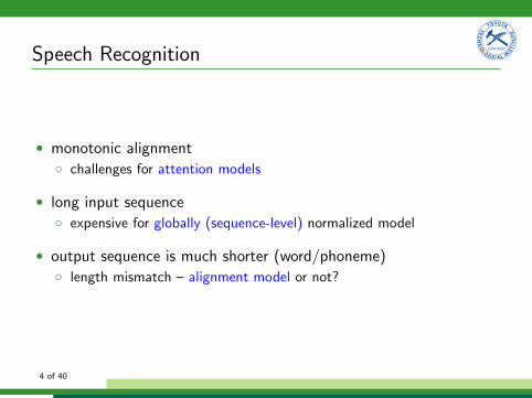
Speech Recognition

• monotonic alignment� challenges for attention models

• long input sequence� expensive for globally (sequence-level) normalized model

• output sequence is much shorter (word/phoneme)� length mismatch – alignment model or not?

4 of 40

Speech Recognition

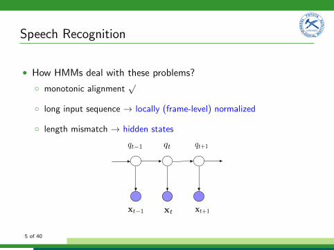
• How HMMs deal with these problems?

� monotonic alignmentp

� long input sequence ! locally (frame-level) normalized

� length mismatch ! hidden states

qt�1 qt qt+1

xt+1xtxt�1

5 of 40

Speech Recognition

• Connectionist Temporal Classification� monotonic alignment

p

� long input sequence ! locally normalized

� length mismatch ! blank state

[1] R. Collobert, et al, “Wav2Letter: an End-to-End ConvNet-based Speech RecognitionSystem”, arXiv 20166 of 40

Speech Recognition

• Attention model

x1 x2 x3 x4 x5

�

y1 y2 y3 y4 y5

Encoder

Attention

Decoder

h1:T = RNN(x1:T )

cj = Attend(h1:T )

P (yj | y1, · · · , yj�1, cj)

7 of 40

Speech Recognition

• Attention model: remarks� monotonic alignment ⇥

� long input sequencep

� length mismatchp

� Locally normalized for each output token

P(y |X ) ⇡Y

j

P(yj |y1, · · · , yj�1, cj) (1)

8 of 40

Speech Recognition

• Locally normalized models:� conditional independence assumption

� label bias problem

� We care more about the sequence level loss in speech recognition

� · · ·

[1] D. Andor, et al, “Globally Normalized Transition-Based Neural Networks”, ACL, 2016

9 of 40

Speech Recognition

• Locally to globally normalized models:� HMMs: CE ! sequence training

� CTC: CE ! sequence training

� Attention model: Minimum Bayes Risk training

L =X

y2⌦

P(y |X )A(y , y) (2)

• Question:Why not sticking to the globally normalised models from scratch?

[1] D. Povey, et al, “Purely sequence-trained neural networks for ASR based on lattice-freeMMI”, Interspeech, 2016[2] S. Shen, et al, “Minimum Risk Training for Neural Machine Translation”, ACL 201610 of 40

(Segmental) Conditional Random Field

CRF segmental CRF

• CRF still require an alignment model for speech recognition

• Segmental CRF is equipped with implicit alignment

11 of 40

(Segmental) Conditional Random Field

• CRF [La↵erty et al. 2001]

P(y1:L | x1:T ) =1

Z (x1:T )

Y

j

exp⇣w

>�(yj , x1:T )⌘

(3)

where L = T .

• Segmental (semi-Markov) CRF [Sarawagi and Cohen 2004]

P(y1:L,E , | x1:T ) =1

Z (x1:T )

Y

j

exp⇣w

>�(yj , ej , x1:T )⌘

(4)

where ej = hsj , nji denotes the beginning (sj) and end (nj) timetag of yj ; E = {e1:L} is the latent segment label.

12 of 40

(Segmental) Conditional Random Field

1Z(x1:T )

Qj exp

�w

>�(yj , x1:T )�

• Learnable parameter w

• Engineering the feature function �(·)

• Designing �(·) is much harder for speech than NLP

13 of 40

Segmental Recurrent Neural Network

• Using (recurrent) neural networks to learn the feature function�(·).

x1 x2 x3 x4

y2y1

x5 x6

y3

14 of 40

Segmental Recurrent Neural Network

• More memory e�cient

x1 x2 x3 x4 x5 x6

y1 y2 y3

copy action copied hidden state

15 of 40

Segmental Recurrent Neural Network

• Comparing to previous segmental models� M. Ostendorf et al., “From HMM’s to segment models: a unified view

of stochastic modeling for speech recognition”, IEEE Trans. Speechand Audio Proc. 1996

� J. Glass, “A probabilistic framework for segment-based speechrecognition”, Computer Speech & Language, 2002

• Markovian framework vs. CRF framework (local vs. globalnormalization)

• Neural network feature (and end-to-end training)

16 of 40

Related works

• (Segmental) CRFs for speech

• Neural CRFs

• Structured SVMs

• Two good review papers�

M. Gales, S. Watanabe and E. Fosler-Lussier, “Structured Discriminative

Models for Speech Recognition”, IEEE Signal Processing Magazine, 2012

�E. Fosler-Lussier et al. “Conditional random fields in speech, audio, and

language processing, Proceedings of the IEEE, 2013

17 of 40

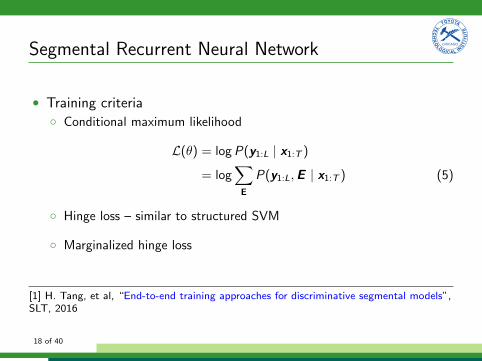
Segmental Recurrent Neural Network

• Training criteria� Conditional maximum likelihood

L(✓) = logP(y1:L | x1:T )

= logX

E

P(y1:L,E | x1:T ) (5)

� Hinge loss – similar to structured SVM

� Marginalized hinge loss

[1] H. Tang, et al, “End-to-end training approaches for discriminative segmental models”,SLT, 2016

18 of 40

Segmental Recurrent Neural Network

• Viterbi decoding� Partially Viterbi decoding

y

⇤1:L = argmax

y1:L

logX

E

P(y1:L,E | x1:T ) (6)

� Fully Viterbi decoding

y⇤1:L,E

⇤ = arg maxy1:L,E

logP(y1:L,E | x1:T ) (7)

19 of 40

Comparison to CTC

[1] A. Senior, et al, “Acoustic Modelling with CD-CTC-sMBR LSTM RNNs”, ASRU 2015.

20 of 40

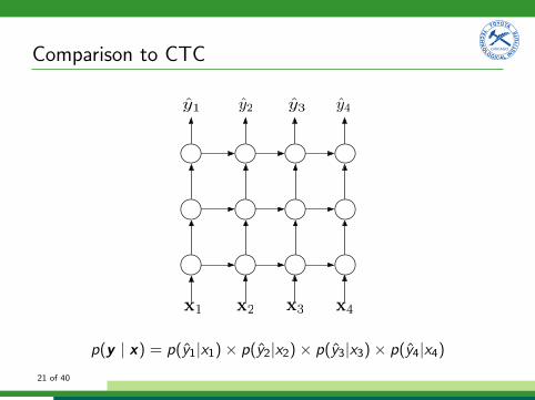
Comparison to CTC

x1 x2 x3 x4

y1 y2 y3 y4

p(y | x) = p(y1|x1) ⇥ p(y2|x2) ⇥ p(y3|x3) ⇥ p(y4|x4)21 of 40

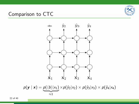
Comparison to CTC

x1 x2 x3 x4

y2 y3 y4<b>

p(y | x) = p(hbi|x1)| {z }⇡1

⇥p(y2|x2) ⇥ p(y3|x3) ⇥ p(y4|x4)

22 of 40

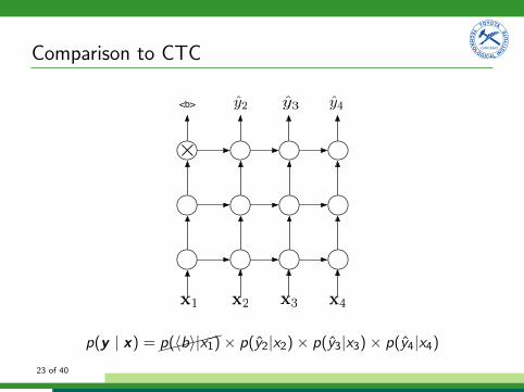
Comparison to CTC

x1 x2 x3 x4

y2 y3 y4<b>

⇥

p(y | x) =⇠⇠⇠⇠⇠p(hbi|x1) ⇥ p(y2|x2) ⇥ p(y3|x3) ⇥ p(y4|x4)23 of 40

Comparison to CTC

x1 x2 x3 x4

y3 y4<b>

⇥

<b>

p(y | x) = p(hbi|x1)| {z }⇡1

⇥ p(hbi|x2)| {z }⇡1

⇥p(y3|x3) ⇥ p(y4|x4)

24 of 40

Comparison to CTC

x1 x2 x3 x4

y3 y4<b>

⇥

<b>

⇥

p(y | x) =⇠⇠⇠⇠⇠p(hbi|x1) ⇥⇠⇠⇠⇠⇠p(hbi|x2) ⇥ p(y3|x3) ⇥ p(y4|x4)25 of 40

Comparison to CTC

x1 x2 x3 x4

y3 y4<b>

⇥

<b>

⇥

26 of 40

Comparison to CTC

x1 x2 x3 x4

y3 y4<b>

⇥

<b>

⇥

• CTC loss may do some kind of segmental modelling

27 of 40

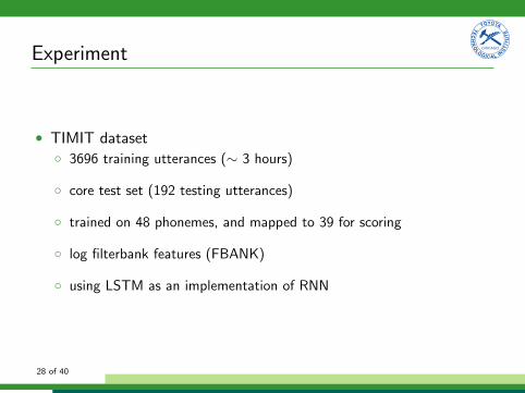
Experiment

• TIMIT dataset� 3696 training utterances (⇠ 3 hours)

� core test set (192 testing utterances)

� trained on 48 phonemes, and mapped to 39 for scoring

� log filterbank features (FBANK)

� using LSTM as an implementation of RNN

28 of 40

Experiment

• Limit the lengths of segments• Recurrent subsampling networks – over 10x speedup

x1 x2 x3 x4· · ·

x1 x2 x3 x4· · ·

a) concatenate / add

b) skip29 of 40

Experiment

• Large model with dropout works the best

Table: Results of dropout.

Dropout layers hidden PER3 128 21.2

0.2 3 250 20.16 250 19.33 128 21.3

0.1 3 250 20.96 250 20.4

⇥ 6 250 21.9

30 of 40

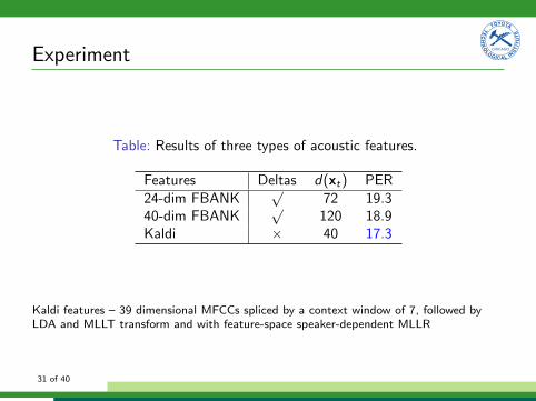
Experiment

Table: Results of three types of acoustic features.

Features Deltas d(xt) PER24-dim FBANK

p72 19.3

40-dim FBANKp

120 18.9Kaldi ⇥ 40 17.3

Kaldi features – 39 dimensional MFCCs spliced by a context window of 7, followed byLDA and MLLT transform and with feature-space speaker-dependent MLLR

31 of 40

Experiment

Table: Comparison to related works. LM = language model, SD = speakerdependent feature

System LM SD PERHMM-DNN

p p18.5

CTC [Graves 2013] ⇥ ⇥ 18.4RNN transducer [Graves 2013] – ⇥ 17.7Attention-based RNN [Chorowski 2015] – ⇥ 17.6Segmental RNN ⇥ ⇥ 18.9Segmental RNN ⇥

p17.3

32 of 40

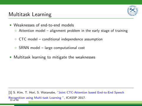
Multitask Learning

• Weaknesses of end-to-end models� Attention model – alignment problem in the early stage of training

� CTC model – conditional independence assumption

� SRNN model – large computational cost

• Multitask learning to mitigate the weaknesses

[1] S. Kim, T. Hori, S. Watanabe, “Joint CTC-Attention based End-to-End Speech

Recognition using Multi-task Learning ”, ICASSP 2017.33 of 40

Multitask Learning

[1] S. Kim, T. Hori, S. Watanabe, “Joint CTC-Attention based End-to-End Speech

Recognition using Multi-task Learning ”, ICASSP 2017.

34 of 40

Multitask Learning

Table: Results of three types of acoustic features.

Model features Dim dev evalSRNN FBANK 250 18.1 20.0+MTL FBANK 250 17.5 18.7

SRNN fMLLR 250 16.6 17.9+MTL fMLLR 250 15.9 17.5

CTC FBANK 250 17.7 19.9+MTL FBANK 250 17.2 18.9

CTC fMLLR 250 16.7 17.8+MTL fMLLR 250 16.2 17.4

[1] L. Lu et al., “Multi-task Learning with CTC and Segmental CRF for Speech

Recognition”, arXiv 2017.

35 of 40

Multitask Learning

0 5 10 15 20

number of epochs

0.35

0.4

0.45

0.5

0.55

0.6

0.65

0.7

0.75

0.8

Err

or

(%)

MTL with CTC pretraining

SRNN with random initialization

MTL with random initialization

[1] L. Lu et al., “Multi-task Learning with CTC and Segmental CRF for Speech

Recognition”, arXiv 2017.

36 of 40

Scale to Large Vocabulary ASR

• Why Segmental CRF expensive?

P(y1:L,E , | x1:T ) =1

Z (x1:T )

Y

j

exp⇣w

>�(yj , ej , x1:T )⌘

(8)

where ej = hsj , nji denotes the beginning (sj) and end (nj) timetag.

Z (x1:T ) =X

y,E

JY

j=1

exp f (yj , ej , x1:T ) . (9)

• Computation complexity is O(T 2|V|)

37 of 40

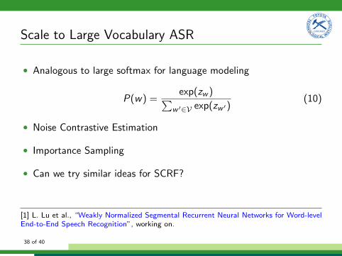
Scale to Large Vocabulary ASR

• Analogous to large softmax for language modeling

P(w) =exp(zw )P

w 02V exp(zw 0)(10)

• Noise Contrastive Estimation

• Importance Sampling

• Can we try similar ideas for SCRF?

[1] L. Lu et al., “Weakly Normalized Segmental Recurrent Neural Networks for Word-levelEnd-to-End Speech Recognition”, working on.

38 of 40

Conclusion

• Segmental CRFs with recurrent neural networks

• Potential for end-to-end speech recognition

• Multi-tasking learning with other end-to-end models

• Large vocabulary tasks

• Other type of neural architectures, e.g. CNNs

39 of 40

Thank you ! Questions?

40 of 40