Segmenting and Tracking the Left Ventricle by

Learning the Dynamics in Cardiac Images?

W. Sun1, M. Cetin1, R. Chan2, V. Reddy2, G. Holmvang2, V. Chandar1, andA. Willsky1

1 Laboratory for Information and Decision Systems,Massachusetts Institute of Technology, Cambridge, MA USA

2 Cardiovascular MR-CT Program, Massachusetts General Hospital,Harvard Medical School, Boston, MA USA

waltsun@mit.edu

Massachusetts Institute of Technology, LIDS Technical Report 2642

February 2005

Abstract. Having accurate left ventricle (LV) segmentations across acardiac cycle provides useful quantitative (e.g. ejection fraction) andqualitative information for diagnosis of certain heart conditions. Exist-ing LV segmentation techniques are founded mostly upon algorithmsfor segmenting static images. In order to exploit the dynamic structureof the heart in a principled manner, we approach the problem of LVsegmentation as a recursive estimation problem. In our framework, LVboundaries constitute the dynamic system state to be estimated, and asequence of observed cardiac images constitute the data. By formulatingthe problem as one of state estimation, the segmentation at each partic-ular time is based not only on the data observed at that instant, but alsoon predictions based on past segmentations. This requires a dynamicalsystem model of the LV, which we propose to learn from training datathrough an information-theoretic approach. To incorporate the learneddynamic model into our segmentation framework and obtain predictions,we use ideas from particle filtering. Our framework uses a curve evolutionmethod to combine such predictions with the observed images to esti-mate the LV boundaries at each time. We demonstrate the effectivenessof the proposed approach on a large set of cardiac images. We observethat our approach provides more accurate segmentations than those fromstatic image segmentation techniques, especially when the observed dataare of limited quality.

1 Introduction

Of the cardiac chambers in the heart, the left ventricle (LV) is quite frequentlyanalyzed because its proper function, pumping oxygenated blood to the entirebody, is vital for normal activity. One quantitative measure of the health of the

? Extended version of IPMI 2005 paper. This work supported by NSF ITR grant0121182 & AFOSR grant FA9550-04-1-0351.

LV is ejection fraction (EF). This statistic measures the percentage volume ofblood transmitted out of the LV in a given cardiac cycle. To compute EF, we needto have segmentations of the LV at multiple points in a cardiac cycle; namely,at end diastole (ED) and end systole (ES). In addition, observing how the LVevolves throughout an entire cardiac cycle allows physicians to determine thehealth of the myocardial muscles. Segmented LV boundaries can also be usefulfor further quantitative analysis. For example, past work [9, 21] on extracting theflow fields of the myocardial wall assumes the availability of LV segmentationsthroughout the cardiac cycle.

Automatic segmentation of the left ventricle (LV) in bright blood breath-hold cardiac magnetic resonance (MR) images is non-trivial because the imageintensities of the cardiac chambers vary due to differences in blood velocity [27].In particular, blood that flows into the ventricles produces higher intensities inthe acquired image than blood which remains in the ventricles [11]. Locating theLV endocardium is further complicated by the fact that the right ventricle andaorta often appear jointly with the LV in many images of the heart. Similarly,automatic segmentation of low signal-to-noise ratio (SNR) cardiac images (e.g.body coil MR or ultrasound) is difficult because intensity variations can oftenobscure the LV boundary.

Several approaches exist for LV segmentation. Goshtasby and Turner [11], aswell as Weng et al. [29] and Geiger et al. [10], apply intensity thresholding andthen a local maximum gradient search to determine the final segmentation. Suchgradient-based methods rely primarily on local information. When the imagestatistics inside an object’s boundary are distinctly different from those outside,the use of region statistics may be more appropriate, especially if the discontinu-ity at the boundary is weak or non-uniform. Tsai et al. [28] consider region-basedsegmentations of the LV. Chakraborty et al. [4] consider combining both gradi-ent and region techniques in the segmentation of cardiac structures. Similarly,Paragios [23] uses gradient and region techniques to segment two cardiac con-tours, the LV endocardium and epicardium. In all three papers, active contours(or curve evolution) [3, 6, 15, 18, 19, 22], a technique which involves evolving acurve to minimize (or maximize) a related objective functional, are used to de-termine the segmentation. In our work, we also take advantage of region-basedinformation and curve evolution.

Static segmentation methods are limited by the data available in an individ-ual frame. During a single cardiac cycle, which lasts approximately 1 second, theheart contracts from end diastole (ED) to end systole (ES) and expands backto ED. Over this time, MR systems can acquire approximately 20 images of theheart. Because adjacent frames are imaged over a short time period (approxi-mately 50 ms), the LV boundaries exhibit strong temporal correlation. Thus,previous LV boundaries may provide information regarding the location of thecurrent LV boundary. Using such information is particularly useful for low SNRimages, where the observation from a single frame alone may not provide enoughinformation for a good segmentation. There exists some past work which simplyuses the previous frame’s LV boundary as the prediction for the boundary in the

current frame [10, 14]. Meanwhile, Zhou et al. [31] consider LV shape trackingby combining predictions, obtained through linear system dynamics assumedknown, with observations. Their technique uses landmark points to representthe LV boundaries, which introduces the issue of correspondence. All uncertain-ties are assumed to be Gaussian. Senegas et al. [24] use a Bayesian frameworkfor tracking using a sample-based approach to estimate the densities. They usespherical harmonics for the shape model, and a simple linear model to approx-imate the cardiac dynamics.3 In our work, we use non-linear dynamics in therecursive estimation of the LV boundary. We represent the LV by level sets toavoid issues inherent with marker points [26] and apply principal componentsanalysis on the level sets to determine a basis to represent the shapes. Further-more, we propose a method for learning a non-trivial dynamic model of the LVboundaries and apply this model to obtain predictions. Finally, we compute themaximum a posteriori (MAP) estimate using curve evolution.

In particular, we propose a principled Bayesian approach for recursively esti-mating the LV boundaries across a cardiac cycle. In our framework, LV bound-aries constitute the dynamic system state we estimate, and a cardiac cycle ofmid-ventricular images constitutes the data. From a training set of data, we learnthe dynamics using an information-theoretic criterion [13]. More specifically, thisinvolves finding a non-parametric density estimate of the current boundary con-ditioned on previous boundaries. The densities are approximately representedby using sample-based (i.e. particle filtering [1]) methods.

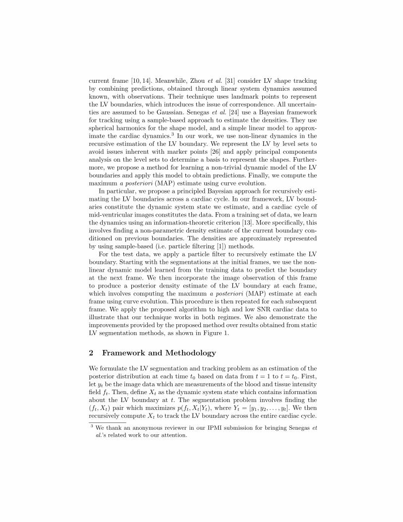
For the test data, we apply a particle filter to recursively estimate the LVboundary. Starting with the segmentations at the initial frames, we use the non-linear dynamic model learned from the training data to predict the boundaryat the next frame. We then incorporate the image observation of this frameto produce a posterior density estimate of the LV boundary at each frame,which involves computing the maximum a posteriori (MAP) estimate at eachframe using curve evolution. This procedure is then repeated for each subsequentframe. We apply the proposed algorithm to high and low SNR cardiac data toillustrate that our technique works in both regimes. We also demonstrate theimprovements provided by the proposed method over results obtained from staticLV segmentation methods, as shown in Figure 1.

2 Framework and Methodology

We formulate the LV segmentation and tracking problem as an estimation of theposterior distribution at each time t0 based on data from t = 1 to t = t0. First,let yt be the image data which are measurements of the blood and tissue intensityfield ft. Then, define Xt as the dynamic system state which contains informationabout the LV boundary at t. The segmentation problem involves finding the(ft,Xt) pair which maximizes p(ft,Xt|Yt), where Yt = [y1, y2, . . . , yt]. We thenrecursively compute Xt to track the LV boundary across the entire cardiac cycle.

3 We thank an anonymous reviewer in our IPMI submission for bringing Senegas etal.’s related work to our attention.

Static Seg Method

Proposed Approach

Static Seg Method

Proposed Approach

(a) (b)

Fig. 1. (a) Segmentation of the fourth frame in the cardiac cycle. (b) Segmentation ofthe eighth frame (near end systole) in the cardiac cycle.

Mathematically, we apply Bayes’ Theorem to the posterior p(ft,Xt|Yt). As-suming that Xt is a Markov process and observing that p(Yt−1) and p(Yt) donot depend on Xt, we have

p(ft,Xt|Yt) ∝ p(yt|ft,Xt)p(ft|Xt)p(Xt|Yt−1) (1)

= p(yt|ft,Xt)p(ft|Xt)

∫

Xt−1

p(Xt|Xt−1)

∫

ft−1

p(ft−1,Xt−1|Yt−1)dft−1dXt−1,

where p(yt|ft,Xt) is the likelihood term, p(ft|Xt) is the field prior, and p(Xt|Yt−1)is the prediction density. From Eqn. (1), we observe the recursive nature of theproblem (i.e. p(ft,Xt|Yt) is written as a function of p(ft−1,Xt−1|Yt−1)).

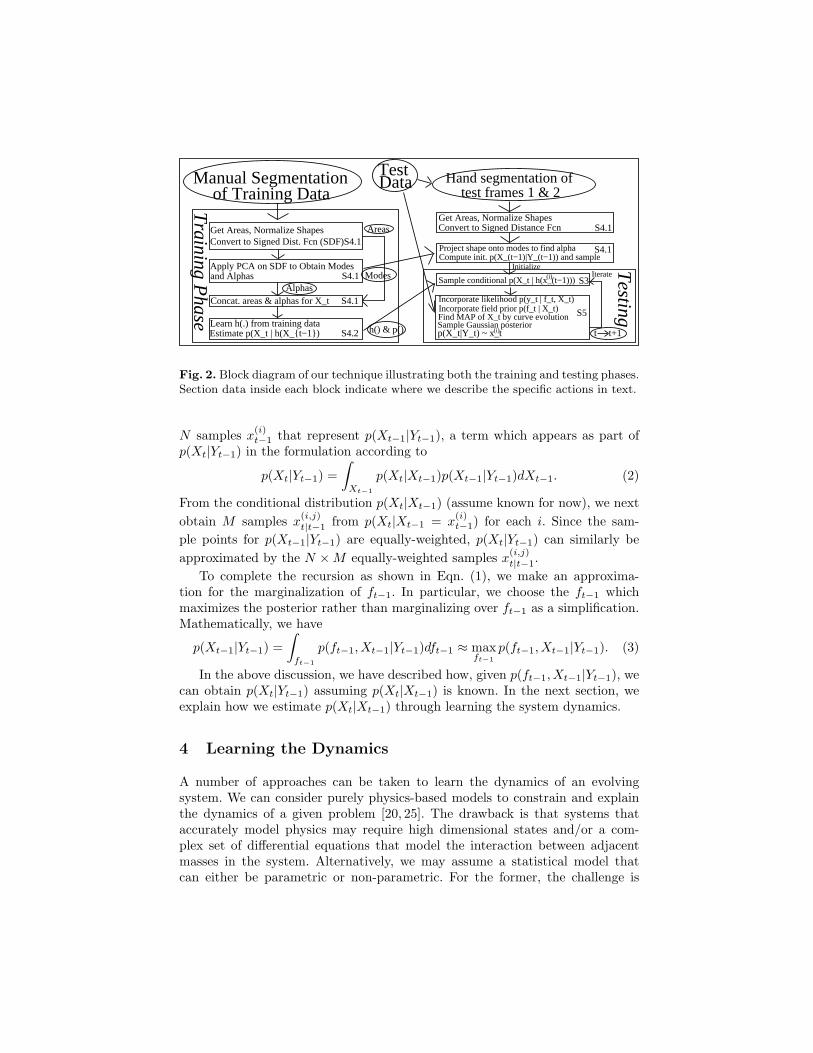
Given this framework, applying it to the LV tracking problem is not straight-forward. One of the challenges involves the presence of arbitrary, non-Gaussianprobability densities. In Section 3, we discuss the use of a sample-based approachto non-parametrically represent the densities in Eqn. (1). In addition, the dy-namic model of the LV boundaries, hence the forward density p(Xt|Xt−1), needsto be learned using statistics from the training data. We discuss the procedure forlearning in Section 4. Finally, we explain in Section 5 how we practically computethe MAP estimate of Xt and use this information to produce a segmentation aswell as an estimate of the posterior p(ft,Xt|Yt). Experimental results are shownin Section 6, and we summarize the work in Section 7. Figure 2 shows a blockdiagram representation of the algorithmic framework we propose.

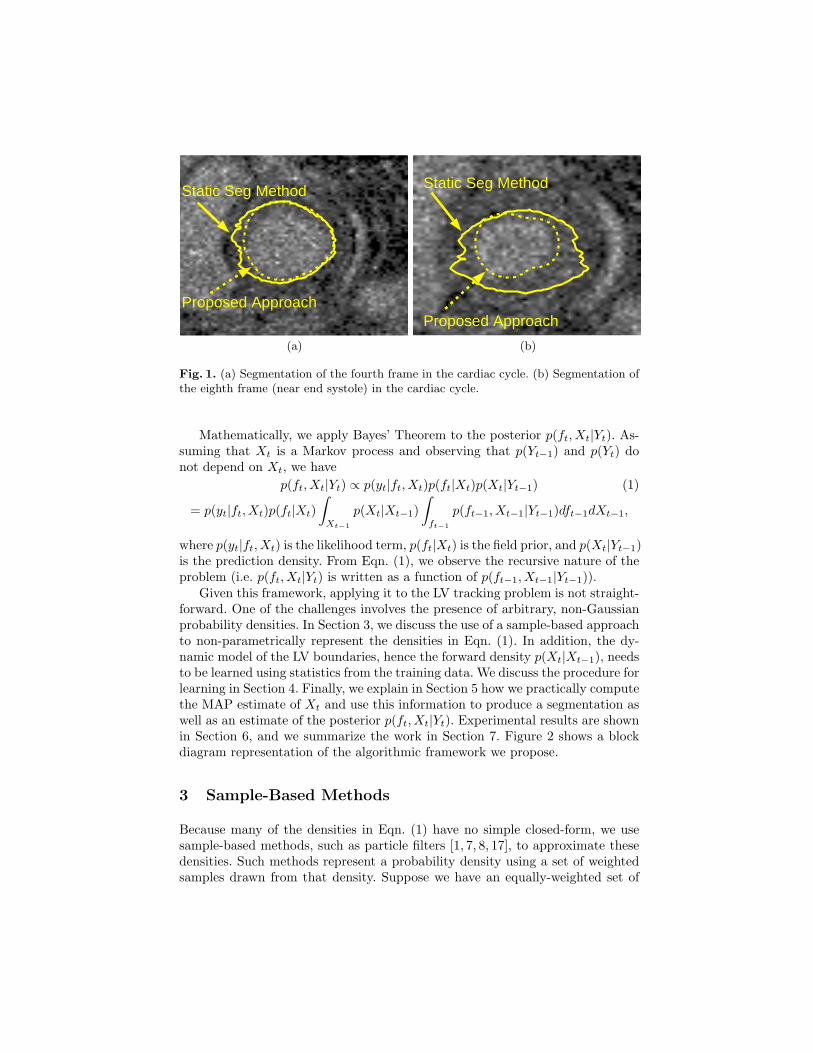
3 Sample-Based Methods

Because many of the densities in Eqn. (1) have no simple closed-form, we usesample-based methods, such as particle filters [1, 7, 8, 17], to approximate thesedensities. Such methods represent a probability density using a set of weightedsamples drawn from that density. Suppose we have an equally-weighted set of

Manual Segmentation

Training P

hase

Apply PCA on SDF to Obtain Modes

Get Areas, Normalize Shapes

and Alphas S4.1

Areas

AlphasConcat. areas & alphas for X_t S4.1

Learn h(.) from training data Estimate p(X_t | h(X_{t−1}) S4.2

Testing

Hand segmentation oftest frames 1 & 2

Get Areas, Normalize ShapesConvert to Signed Distance Fcn

Modes

Project shape onto modes to find alphaCompute init. p(X_(t−1)|Y_(t−1)) and sample

S4.1

Sample conditional p(X_t | h(x_(t−1)))

h() & p() (i)

(i)

Incorporate likelihood p(y_t | f_t, X_t)

Find MAP of X_t by curve evolution S5Sample Gaussian posteriorp(X_t|Y_t) ~ x_t

S3

t t+1

Convert to Signed Dist. Fcn (SDF)S4.1

of Training Data

Initialize

Incorporate field prior p(f_t | X_t)

Iterate

S4.1

TestData

Fig. 2. Block diagram of our technique illustrating both the training and testing phases.Section data inside each block indicate where we describe the specific actions in text.

N samples x(i)t−1 that represent p(Xt−1|Yt−1), a term which appears as part of

p(Xt|Yt−1) in the formulation according to

p(Xt|Yt−1) =

∫

Xt−1

p(Xt|Xt−1)p(Xt−1|Yt−1)dXt−1. (2)

From the conditional distribution p(Xt|Xt−1) (assume known for now), we next

obtain M samples x(i,j)t|t−1 from p(Xt|Xt−1 = x

(i)t−1) for each i. Since the sam-

ple points for p(Xt−1|Yt−1) are equally-weighted, p(Xt|Yt−1) can similarly be

approximated by the N × M equally-weighted samples x(i,j)t|t−1.

To complete the recursion as shown in Eqn. (1), we make an approxima-tion for the marginalization of ft−1. In particular, we choose the ft−1 whichmaximizes the posterior rather than marginalizing over ft−1 as a simplification.Mathematically, we have

p(Xt−1|Yt−1) =

∫

ft−1

p(ft−1,Xt−1|Yt−1)dft−1 ≈ maxft−1

p(ft−1,Xt−1|Yt−1). (3)

In the above discussion, we have described how, given p(ft−1,Xt−1|Yt−1), wecan obtain p(Xt|Yt−1) assuming p(Xt|Xt−1) is known. In the next section, weexplain how we estimate p(Xt|Xt−1) through learning the system dynamics.

4 Learning the Dynamics

A number of approaches can be taken to learn the dynamics of an evolvingsystem. We can consider purely physics-based models to constrain and explainthe dynamics of a given problem [20, 25]. The drawback is that systems thataccurately model physics may require high dimensional states and/or a com-plex set of differential equations that model the interaction between adjacentmasses in the system. Alternatively, we may assume a statistical model thatcan either be parametric or non-parametric. For the former, the challenge is

Fig. 3. Illustration of LV shape variability. ±1σ for the first eight primary modes ofvariability (left to right). Solid curve represents +1σ while dashed represents −1σ.

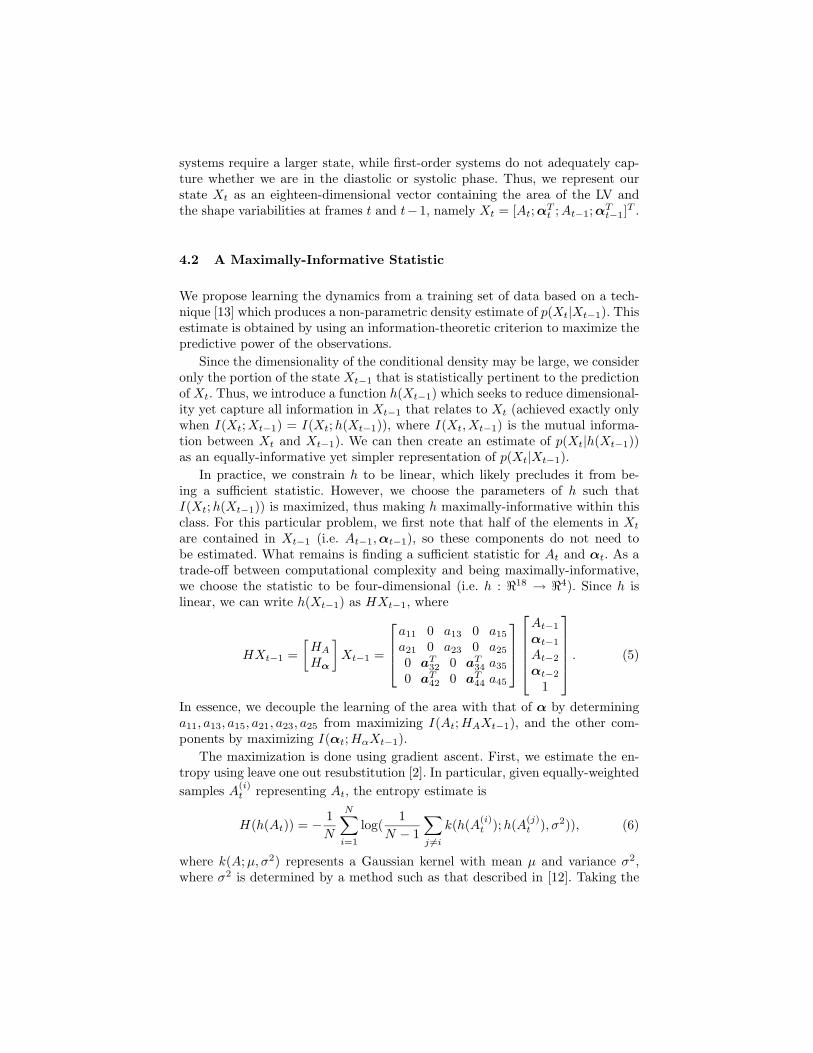
to find a parametric model that is well-matched to the problem structure andcaptures the statistical variability inherent in the problem. For richer modelingcapacity, one can turn to non-parametric models, which can be computation-ally difficult. In Section 4.2, we explain our non-parametric, yet computationallytractable approach to learning the dynamics of LV boundaries. Before discussingthis method, we first provide a description of the system state Xt.

4.1 Implicit Parametric Shape Model and State Representation

The set of LV boundaries have different internal areas and different shapes acrossa cardiac cycle and between patients. We want to represent these boundaries ina simple, low-dimensional, yet accurate, manner. To accomplish this, we useprincipal components analysis (PCA) on the shape variability to obtain a basisfor the shapes [19]. We then represent each shape by a linear combination of thebasis elements. The tracking problem reduces to learning the time evolution ofthe coefficients of the basis elements.

Starting with a training set of manually-segmented and registered data, wedetermine the area of each LV. Normalizing with respect to area, we createsigned distance functions whose zero level sets are the shapes [26]. Leveragingon Leventon’s PCA on shapes [19], we obtain a mean shape ψ and the primarymodes of variability ψi (for i=1,2, . . . , K, where K is the number of shapes inthe dataset) across the entire training set. In effect, we use a single basis torepresent the shapes across the entire cardiac cycle. Figure 3 shows the eightprimary modes of variability from the training set used in the experimentalresults presented in Section 6. For a given signed distance function ψ in thetraining set,

ψ = ψ +K

∑

i=1

αiψi, (4)

where αi’s are a set of constants. It is known that for shapes which do not varygreatly, the primary few modes of variability can explain the majority of thevariability of the data. In our training set, the first eight modes explain 97%of the variability in our specific training set of data. Thus, we approximatelyrepresent each ψ by the eight element vector α = [α1;α2; . . . ;α8]

T . By usingPCA, a given curve (LV segmentation) can be approximately represented by avector containing its area A and α.

Given this representation, we define the state Xt with the notion that thedynamics are a second-order system. This choice is made because higher-order

systems require a larger state, while first-order systems do not adequately cap-ture whether we are in the diastolic or systolic phase. Thus, we represent ourstate Xt as an eighteen-dimensional vector containing the area of the LV andthe shape variabilities at frames t and t−1, namely Xt = [At;α

Tt ;At−1;α

Tt−1]

T .

4.2 A Maximally-Informative Statistic

We propose learning the dynamics from a training set of data based on a tech-nique [13] which produces a non-parametric density estimate of p(Xt|Xt−1). Thisestimate is obtained by using an information-theoretic criterion to maximize thepredictive power of the observations.

Since the dimensionality of the conditional density may be large, we consideronly the portion of the state Xt−1 that is statistically pertinent to the predictionof Xt. Thus, we introduce a function h(Xt−1) which seeks to reduce dimensional-ity yet capture all information in Xt−1 that relates to Xt (achieved exactly onlywhen I(Xt;Xt−1) = I(Xt;h(Xt−1)), where I(Xt,Xt−1) is the mutual informa-tion between Xt and Xt−1). We can then create an estimate of p(Xt|h(Xt−1))as an equally-informative yet simpler representation of p(Xt|Xt−1).

In practice, we constrain h to be linear, which likely precludes it from be-ing a sufficient statistic. However, we choose the parameters of h such thatI(Xt;h(Xt−1)) is maximized, thus making h maximally-informative within thisclass. For this particular problem, we first note that half of the elements in Xt

are contained in Xt−1 (i.e. At−1,αt−1), so these components do not need tobe estimated. What remains is finding a sufficient statistic for At and αt. As atrade-off between computational complexity and being maximally-informative,we choose the statistic to be four-dimensional (i.e. h : <18 → <4). Since h islinear, we can write h(Xt−1) as HXt−1, where

HXt−1 =

[

HA

Hα

]

Xt−1 =

a11 0 a13 0 a15

a21 0 a23 0 a25

0 aT32 0 a

T34 a35

0 aT42 0 a

T44 a45

At−1

αt−1

At−2

αt−2

1

. (5)

In essence, we decouple the learning of the area with that of α by determininga11, a13, a15, a21, a23, a25 from maximizing I(At;HAXt−1), and the other com-ponents by maximizing I(αt;HαXt−1).

The maximization is done using gradient ascent. First, we estimate the en-tropy using leave one out resubstitution [2]. In particular, given equally-weighted

samples A(i)t representing At, the entropy estimate is

H(h(At)) = − 1

N

N∑

i=1

log(1

N − 1

∑

j 6=i

k(h(A(i)t );h(A

(j)t ), σ2)), (6)

where k(A;µ, σ2) represents a Gaussian kernel with mean µ and variance σ2,where σ2 is determined by a method such as that described in [12]. Taking the

derivative with respect to each of the parameters aij , we obtain

∂H

∂amn

= − 1

N=

N∑

i=1

[1

∑

j 6=i k(h(A(i)t );h(A

(j)t ), σ2)

∑

j 6=i

−h(A(i)t ) − h(A

(j)t )

σ2k(h(A

(i)t );h(A

(j)t , σ2))(

∂h(A(i)t )

∂amn

− ∂h(A(j)t )

∂amn

)]. (7)

Given that the mutual information between At and h(At−1) is defined as

I(At;h(At−1)) = H(At) + H(h(At−1)) − H(At, h(At−1)), (8)

we can find the gradient of I(At;h(At−1)) by applying Equation (7) to the secondand third terms (the first term is independent of h). At each iteration, we move inthe direction of the gradient, continuing until convergence. Once the parametersof h are determined, we obtain a kernel density estimate of p(Xt|h(Xt−1)), wherefor kernel size we use the plug-in method of Hall et al. [12].

5 Finding the MAP Estimate by Curve Evolution

Now, we incorporate the data at time t to obtain the posterior p(ft,Xt|Yt).

Given equally-weighted samples x(i,j)t|t−1 for p(Xt|Yt−1) as described in Section 3,

one could in principle weight the particles by the likelihood and field priorsto obtain a representation of p(ft,Xt|Yt). Such an approach may work if thetraining data are rich. However, when we have a limited amount of training data,we make the assumption that the posterior distribution of Xt is Gaussian anddetermine this distribution by first computing its MAP estimate to determinethe mean parameter (since we do not have a method in place to compute theposterior covariance, we approximate it to be a diagonal matrix with individualvariances determined empirically from the shape variability in the training data).Maximizing p(ft,Xt|Yt) to obtain the MAP estimate is equivalent to minimizing

E(ft,Xt) = −log p(yt|ft,Xt) − log p(ft|Xt) − log p(Xt|Yt−1), (9)

which involves a likelihood term p(yt|ft,Xt), the prior on the field p(ft|Xt), anda prediction term p(Xt|Yt−1). We discuss each term in Eqn. (9) individually.

5.1 Likelihood Term

Because we are interested in locating the boundary, we apply a simple obser-vation model which assumes that the intensities are piecewise constant, witha bright intensity representing blood and a darker one representing the my-ocardium. Intensity variations in the observation, such as those due to differ-ences in blood velocity [11], are modeled through a multiplicative random field(other choices of noise models can be handled in our framework, with the resultbeing a different observation model). Mathematically, the observation model is

yt(z) =

{

fRin(Xt)t · n(z) , z ∈ Rin(Xt)

fRout(Xt)t · n(z) , z ∈ Rout(Xt),

(10)

where fRin(Xt)t and f

Rout(Xt)t are the constant, but unknown, field intensities

for the blood pool region inside, Rin, and the myocardial region immediatelyoutside (within five pixels), Rout, of the LV boundary, respectively, and n(z)is spatially independent, identically distributed lognormal random field withlog n(z) a Gaussian random variable having zero mean and variance σ2

n. Notethat we explicitly indicate the dependence of the regions on Xt. Given the field

intensity fR(Xt)t and the observation model of Eqn. (10), log yt(z) is normally

distributed with mean log fR(Xt)t and variance σ2

n. Thus,

p(yt|ft,Xt) ∝ (11)

exp( −∫

z∈Rin(Xt)

(log yt(z) − log fRin(Xt)t )2

2σ2n

dz −∫

z∈Rout(Xt)

(log yt(z) − log fRout(Xt)t )2

2σ2n

dz).

Since we have a second order model, Xt contains LV boundary information atboth t and t−1. For the likelihood term, the regions Rin and Rout are determinedby the boundary information from time t.

5.2 Field Priors

In applications where it is possible to extract prior field information, we incorpo-rate a field prior into the problem. The mean log intensity inside is approximatelystationary across a cardiac cycle. We can compute the mean and variance of thelog intensity inside (u and σ2

u, resp.) and that immediately outside the curve (vand σ2

v , resp.) from the training data. We use this information as a prior on thefield ft. Specifically, we have

p(ft|Xt) ∝ exp(− (log fRin

t − u)2

2σ2u

)exp(− (log fRout

t − v)2

2σ2v

). (12)

5.3 Prediction Term

Next, we want to provide a model for the prediction term. In Section 3, we

described having equally-weighted samples x(i,j)t|t−1 to approximately represent

our prediction term p(Xt|Yt−1). We model this prediction density with a Parzendensity estimate using these sample points. Mathematically,

p(Xt|Yt−1) =1

MN

∑

(i,j)

k(Xt;x(i,j)t|t−1, σ

2) =1

MN

∑

(i,j)

1√2πσ

exp(−d2(Xt, x

(i,j)t|t−1)

2σ2),

(13)where k(X;µ, σ2) represents a Gaussian kernel with mean µ and variance σ2 asdetermined from the bandwidth [12], MN is the number of samples, and d(Xt, x)is a distance measure between Xt and sample x (as described below).

5.4 Curve Evolution

Having the likelihood, prediction, and prior as above, and defining F it (Xt) =

log fRin(Xt)t and F o

t (Xt) = log fRout(Xt)t , Eqn. (9) becomes

E(ft,Xt) = α(

∫

z∈Rin(Xt)

(log yt(z) − F it (Xt))

2

2σ2n

dz +

∫

z∈Rout(Xt)

(log yt(z) − F ot (Xt))

2

2σ2n

dz)

+β((F i

t (Xt) − u)2

2σ2u

+(F o

t (Xt) − v)2

2σ2v

)+γ log(1

MN

∑

(i,j)

1√2πσ

exp(−d2(Xt, x

(i,j)t|t−1)

2σ2)),

(14)where α, β, γ are weighting parameter specified based on the quality of data. Forinstance, in low SNR images, α is less heavily-weighted relative to β and γ.

To find the (ft,Xt) pair which minimizes E(ft,Xt) (which only involves theAt and αt variables in Xt), we first consider minimizing E(ft,Ct), the samefunctional but generalized to allow for any curve Ct in the image space <2

rather than the space spanned by At and αt. Eqn. (14) generalizes to

E(ft,Ct) = α(

∫

z∈Rin(Ct)

(log yt(z) − F it (Ct))

2

2σ2n

dz +

∫

z∈Rout(Ct)

(log yt(z) − F ot (Ct))

2

2σ2n

dz)

+β((F i

t (Ct) − u)2

2σ2u

+(F o

t (Ct) − v)2

2σ2v

)+γ log(1

MN

∑

(i,j)

1√2πσ

exp(−d2(Ct, x

(i,j)t|t−1)

2σ2)),

(15)where the distance d(Ct, xt|t−1) is defined to be the line integral along Ct,according to

∮

Ct

D2(s, xt|t−1)ds, with D(s, x) being the Euclidean distance of apoint s from the curve defined by At and αt of xt.

Once Ct is determined, we project it onto the PCA space described in Sec-tion 4.1, yielding At and αt, which given At−1 and αt−1, provides XMAP

t as theMAP estimate for Xt. We use XMAP

t to approximate the state which minimizesE(ft,Xt). We now describe how we use curve evolution to minimize E(ft,Ct)over <2.

Curve evolution methods evolve curves to minimize an associated energyfunctional by incorporating constraints from available data (e.g. imagery). Math-ematically, this amounts to determining

C = argminC

[E(C)], (16)

where C represents the segmentation and E is the energy functional to be mini-mized. If we introduce an iteration time parameter τ (at each time t, we iterateover an artificial and unrelated time τ to find a solution), we may evolve ourcurve according to a differential equation of the form

∂C

∂τ= −F(C), (17)

where F(C) is a force functional. Choosing F(C) as the first variation of E(C)allows the curve to move in the direction of steepest descent. The curve is evolveduntil steady-state is reached (i.e. F(C) = 0).

E(ft,Ct) depends on two variables. To find ft and Ct which minimize E, weuse the technique of coordinate descent. Using this approach, we divide each iter-ation into two steps. First, we fix Ct and find the ft which minimizes E(ft,Ct).Then, we fix ft and evolve Ct in the direction of the first variation of E(ft,Ct)with respect to Ct. The first variation of Eqn. (15) is

∂Ct

∂τ(z) = −[α(F o

t (Ct) − F it (Ct))(2 log yt(z) − F o

t (Ct) − F it (Ct))

+2β(F i

t (Ct) − u)

Ain

(F it (Ct) − log yt(z)) + 2β

(F ot (Ct) − v)

Aout

(F ot (Ct) − log yt(z))

+γ1

K

∑

(i,j)

1√2πσ

exp(−d2(Ct, x

(i,j)t|t−1)

2σ2)(∇D2(z, x

(i,j)t|t−1)·N+D2(z, x

(i,j)t|t−1)κ(z))]N ,

(18)where K = p(Ct|Yt−1)MNσ2, Ain is the area of Rin and Aout is the area ofRout, κ(z) is the curvature of C at z, and N is the unit outward normal of C

at z. The computation of the first variation relies on four separate derivationsof curve flows [5, 6, 16, 30].

6 Experimental Results

We apply the proposed technique on 2-D mid-ventricular slices of data, althoughit is also applicable to 3-D with a corresponding increase in computational com-plexity. The dataset we use contains twenty frame time sequences of breath-holdcardiac MR images, each representing a single cardiac cycle. We do not considerarrhythmia because only patients having sustained and hemodynamically-stablearrhythmia can be practically imaged and analyzed. Such a condition is veryrare. Anonymized data sets of were obtained from the Cardiovascular MR-CTProgram at Massachusetts General Hospital.

6.1 Training

As discussed in Section 4.1, we represent each manually segmented LV from thetraining set (a total of 840 frames) by a shape variability vector α and an area A.We obtain the state Xt for each frame t in the cardiac cycle. Then, we learn thedynamics of our system by maximizing I(Xt;h(Xt−1)), where we approximate h

by a linear function, and use gradient ascent on the parameters of h to find themaximum. We obtain a density estimate of p(Xt|h(Xt−1)) for use in test data.

6.2 Testing

We take sequences of twenty frames (ones not included in the training set),each a single cardiac cycle, as input for testing. For initialization, we assumethat a user provides a segmentation of the first two frames in the sequence.The segmentations can be approximate segmentations using some automated

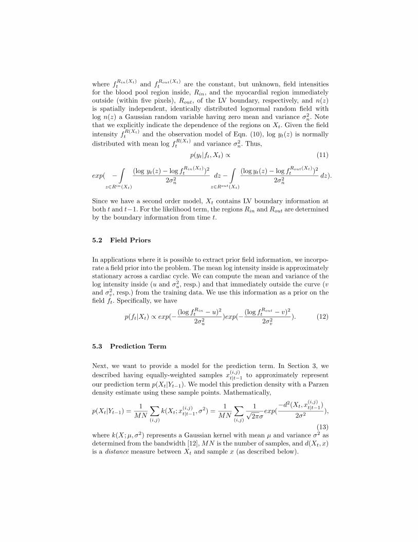
Fig. 4. Curves representing predictions of the LV segmentation (observed MR imagein the background) for frames 3 to 20, shown in raster scan, of a full cardiac cycle.

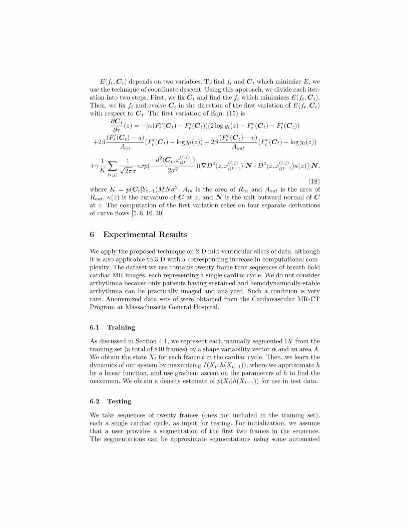
Fig. 5. Segmentations of MR images by obtaining the MAP estimate of Xt.

method, a hand-segmentation by an expert, or predicted using a segmentationfrom a neighboring 2-D slice of the same patient at the same time. From thesesegmentations, we obtain the initial posterior p(f2,X2|Y2). Using particle filtersand curve evolution as described, we recursively estimate the posterior for eachframe in the cardiac cycle.

6.3 Results

In Figure 4, we show samples of the forward prediction p(Xt|h(Xt−1)) for frames3 to 20 in the cardiac cycle. Note that these predictions are obtained basedon segmentations from previous frames and on the learned dynamic model, butbefore incorporating the data shown in the background. Figure 5 shows the MAPestimates of Xt, which involves incorporating the observed data. This estimateis obtained by minimizing Eqn. (14) and provides what qualitatively appears tobe a reasonable segmentation of the LV boundary. Quantitatively, we measureaccuracy by computing the symmetric difference between the segmentation andthe manually-segmented truth normalized by the area of truth. Here, the average

Fig. 6. Curves representing samples of the posterior density p(ft, Xt|Yt) (curves aretightly overlaid on top of each other).

value across the cardiac cycle of test data is 0.04. Finally, Figure 6 shows equally-weighted samples of the posterior density p(Xt|Yt) for each t. This example showsgood segmentation results, but since the quality of the images are very good,static segmentation methods yield results similar to those shown in Figure 5.

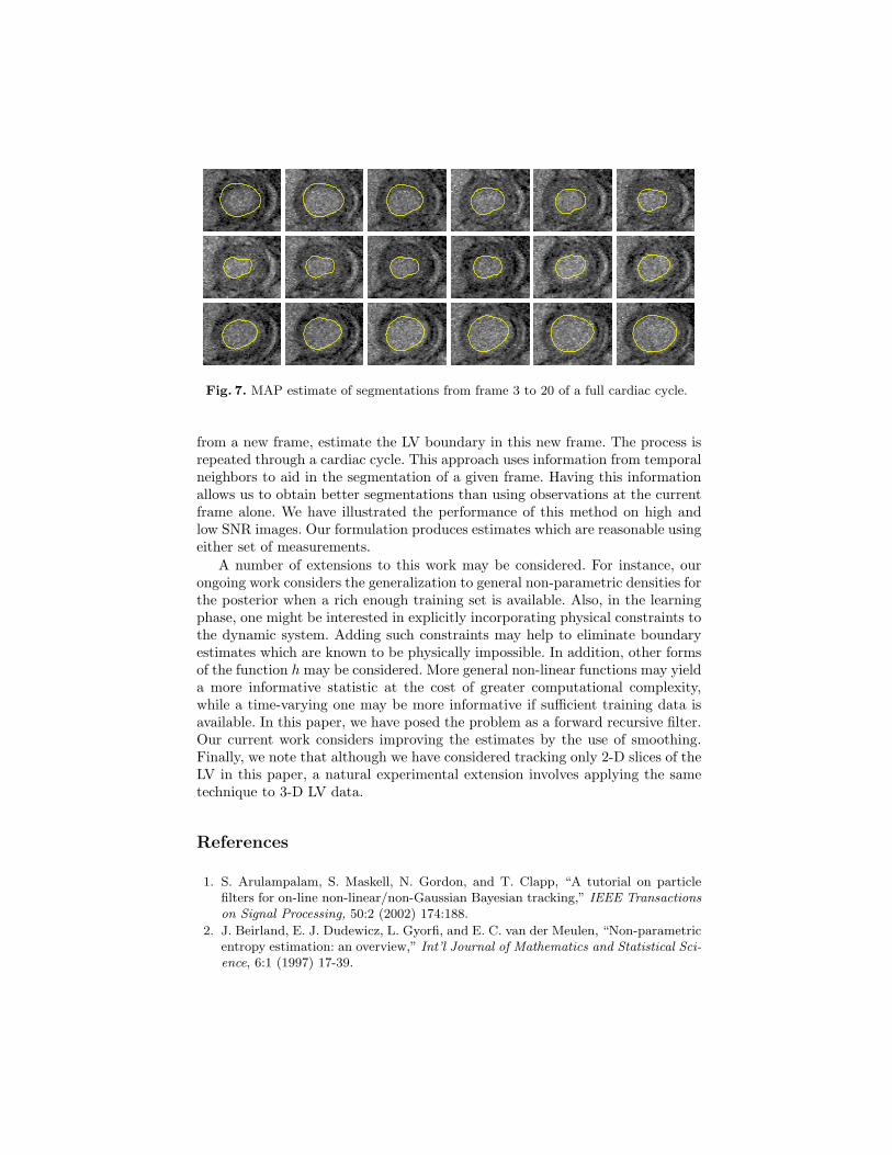
We now consider low SNR images where static segmentation may not pro-duce reasonable results. To simulate low SNR conditions, we add independent,lognormal multiplicative noise to MR images to produce a noisy dataset. Usingdynamics trained from the MR image training set and initializing again usinghand-segmentations on the first two frames, we estimate the LV boundaries. Fig-ure 7 shows segmentations for a full cardiac cycle by taking the MAP estimateof Xt overlaid on the corresponding noisy MR data. Visually, the segmentationsappear to provide accurate localizations of the LV boundaries despite the lowquality data.

In Figure 1, we have provided a visual comparison between our approachand one using static segmentation. The two frames shown are representativeof the results obtained throughout the cardiac cycle. Quantitatively across theentire cardiac cycle, the normalized symmetric difference from our approach is0.08, while that for static segmentation is 0.17. The static segmentation methodis obtained by replacing the p(Xt|Yt−1) term in our formulation with a curvelength prior and is similar to the region-based segmentation methods described inthe introduction [4, 23, 28]. In both illustrations, incorporating dynamics into thesegmentation process using the approach we propose results in better estimatesthan those using a static segmentation method.

7 Conclusion

We have proposed a principled method to recursively estimate the LV boundaryacross a cardiac cycle. In the training phase, we learn the dynamics of the LVby obtaining a non-parametric density estimate for the system dynamics. Fromthis, we produce predictions which, used in conjunction with the observations

Fig. 7. MAP estimate of segmentations from frame 3 to 20 of a full cardiac cycle.

from a new frame, estimate the LV boundary in this new frame. The process isrepeated through a cardiac cycle. This approach uses information from temporalneighbors to aid in the segmentation of a given frame. Having this informationallows us to obtain better segmentations than using observations at the currentframe alone. We have illustrated the performance of this method on high andlow SNR images. Our formulation produces estimates which are reasonable usingeither set of measurements.

A number of extensions to this work may be considered. For instance, ourongoing work considers the generalization to general non-parametric densities forthe posterior when a rich enough training set is available. Also, in the learningphase, one might be interested in explicitly incorporating physical constraints tothe dynamic system. Adding such constraints may help to eliminate boundaryestimates which are known to be physically impossible. In addition, other formsof the function h may be considered. More general non-linear functions may yielda more informative statistic at the cost of greater computational complexity,while a time-varying one may be more informative if sufficient training data isavailable. In this paper, we have posed the problem as a forward recursive filter.Our current work considers improving the estimates by the use of smoothing.Finally, we note that although we have considered tracking only 2-D slices of theLV in this paper, a natural experimental extension involves applying the sametechnique to 3-D LV data.

References

1. S. Arulampalam, S. Maskell, N. Gordon, and T. Clapp, “A tutorial on particlefilters for on-line non-linear/non-Gaussian Bayesian tracking,” IEEE Transactionson Signal Processing, 50:2 (2002) 174:188.

2. J. Beirland, E. J. Dudewicz, L. Gyorfi, and E. C. van der Meulen, “Non-parametricentropy estimation: an overview,” Int’l Journal of Mathematics and Statistical Sci-ence, 6:1 (1997) 17-39.

3. V. Caselles, F. Catte, T. Coll, and F. Dibos, “A geometric model for active contoursin image processing,” Numerische Mathematik, 66 (1993) 1-31.

4. A. Chakraborty, L. Staib, and J. Duncan, “Deformable boundary finding in medicalimages by integrating gradient and region information,” IEEE Transactions onMedical Imaging, 15 (1996) 859-870.

5. T. F. Chan and L. A. Vese, “Active contours without edges,” IEEE Transactionson Image Processing, 10:2 (2001) 266-277.

6. Y. Chen, H. D. Tagare, S. Thiruvenkadam, F. Huang, D. Wilson, K. S. Gopinath,and R. W. Briggs, “Using prior shapes in geometric active contours in a variationalframework,” Int’l Journal of Computer Vision, 50:3 (2002) 315-328.

7. A. Doucet, S. J. Godsill, and C. Andrieu, “On sequential Monte Carlo samplingmethods for Bayesian filtering,” Statistics and Computing, 10:3 (2000) 197-208.

8. P. M. Djuric, J. H. Kotecha, J. Zhang, Y. Huang, T. Ghirmi, M. F. Bugallo, and J.Miguez, “Particle filtering,” IEEE Signal Processing Magazine, 20:5 (2003) 19-38.

9. J. S. Duncan, A. Smeulders, F. Lee, and B. Zaret, “Measurement of end diastolicshape deformity using bending energy,” in Computers in Cardiology, (1988) 277-280.

10. D. Geiger, A. Gupta, L. A. Costa, and J. Vlontzos, “Dynamic programming fordetecting, tracking and matching deformable contours,” IEEE Transactions onPattern Analysis and Machine Intelligence, 17:3 (1995) 294-302.

11. A. Goshtasby and D. A. Turner, “Segmentation of cardiac cine MR images forextraction of right and left ventricular chambers,” IEEE Transactions on MedicalImaging, 14:1 (1995) 56-64.

12. P. Hall, S. J. Sheather, M. C. Jones, and J. S. Marron, “On optimal data-basedbandwidth selection in kernel density estimation,” Biometrika, 78:2 (1991) 263-269.

13. A. Ihler, “Maximally informative subspaces: nonparametric estimation for dynam-ical systems,” M. S. Thesis, Massachusetts Institute of Technology (2000).

14. M-P. Jolly, N. Duta, and G. Funka-Lea, “Segmentation of the left ventricle incardiac MR images,” Proceedings of the Eighth IEEE Int’l Conference on ComputerVision, 1 (2001) 501-508.

15. M. Kass, A. Witkin, and D. Terzopoulos, “Snakes: Active contour models,” Int’lJournal of Computer Vision, (1987) 321-331.

16. J. Kim, “Nonparametric statistical methods for image segmentation and shapeanalysis,” Ph. D. Thesis, Massachusetts Institute of Technology (2005).

17. J. H. Kotecha and P. M. Djuric, “Gaussian particle filtering,” IEEE Transactionson Signal Processing, 51:10 (2003) 2592-2601.

18. G. Kuhne, J. Weickert, O. Schuster, and S. Richter, “A tensor-driven active con-tour model for moving object segmentation,” Proceedings of the 2001 IEEE Int’lConference on Image Processing, 2 (2001) 73-76.

19. M. Leventon, E. Grimson, and O. Faugeras, “Statistical shape influence in geodesicactive contours,” Proceedings of the IEEE Conference on Computer Vision andPattern Recognition, 1 (2000) 316-323.

20. A. McCulloch, J. B. Bassingthwaighte, P. J. Hunter, D. Noble, T. L. Blundell,and T. Pawson, “Computational biology of the heart: From structure to function,”Progress in Biophysics and Molecular Biology, 69:2-3 (1998) 151-559.

21. J. C. McEachen II and J. S. Duncan, “Shape-based tracking of left ventricular wallmotion,” IEEE Transactions on Medical Imaging, 16:3 (1997) 270-283.

22. N. Paragios and R. Deriche, “Geodesic Active Contours and Level Sets for the De-tection and Tracking of Moving Objects,” IEEE Transactions on Pattern Analysisand Machine Intelligence, 22 (2000) 266-280.

23. N. Paragios, “A variational approach for the segmentation of the left ventricle incardiac image analysis,” Int’l Journal of Computer Vision, 50:3 (2002) 345-362.

24. J. Senegas, T. Netsch, C. A. Cocosco, G. Lund, and A. Stork, “Segmentation ofMedical Images with a Shape and Motion Model: A Bayesian Perspective,” Com-puter Vision Approaches to Medical Image Analysis (CVAMIA) and MathematicalMethods in Biomedical Image Analysis (MMBIA) Workshop, (2004) pp. 157-168.

25. M. Sermesant, C. Forest, X. Pennec, H. Delingette, and N. Ayache, “Deformablebiomechanical models: Applications to 4D cardiac image analysis,” Medical ImageAnalysis, 7:4 (2003) 475-488.

26. J. A. Sethian, “Level Set Methods: Evolving Interfaces in Geometry, Fluid Me-chanics, Computer Vision, and Material Science,” Cambridge Univ. Press, 1996.

27. G. K. von Schutthess, “The effects of motion and flow on magnetic resonanceimaging,” In Morphology and Function in MRI, Ch. 3 (1989) 43-62.

28. A. Tsai, A. Yezzi, W. Wells, C. Tempany, D. Tucker, A. Fan, W. E. Grimson,and A. Willsky, “A shape-based approach to the segmentation of medical imageryusing level sets,” IEEE Transactions on Medical Imaging, 22:2 (2003) 137-154.

29. J. Weng, A. Singh, and M. Y. Chiu, “Learning-based ventricle detection fromcardiac MR and CT images,” IEEE Transactions on Medical Imaging, 16:4 (1997)378-391.

30. A. Yezzi, A. Tsai, and A. Willsky, “A fully global approach to image segmentationvia coupled curve evolution equations,” Journal of Vision Communication andImage Representation, 13 (2002) 195-216.

31. X. S. Zhou, D. Comaniciu, and A. Gupta, “An information fusion framework forrobust shape tracking,” IEEE Transactions on Pattern Analysis and Machine In-telligence, 27:1 (2005) 115-129.