Seismic Acquisition with Ocean Bottom Nodes Providing full azimuth seismic images in busy oilfields 20 April 2011 Bjorn Olofsson, Seabird Exploration Abstract: Ocean bottom seismometers have been used by academia for several decades to study mostly the deep subsurface. But only since recently, such ocean bottom nodes (OBN) have been used in commercial seismic surveys for oil & gas exploration and development. In the 1990s the first 2D case studies using OBNs were carried out in the North Sea, and more substantial 2D & 3D pilot surveys followed in the early 2000s in the Gulf of Mexico, the North Sea, and in West Africa. The first full 3D OBN survey was carried out in 2004/2005 in the southern Gulf of Mexico, and until 2008 only one or maximum two 3D OBN survey per year were acquired world-wide. Since 2008, about 12 OBN surveys have been acquired world-wide, and demand for 2011 onwards is increasing. Why are OBNs chosen in favor of towed streamer or ocean bottom cables? The main driver is the full azimuth information achieved with a typical OBN survey design which enables best illumination and imaging in complex structure, for example sub-salt and sub-basalt. Another equally important driver has been the need to acquire seismic data in congested oilfields: Oilfields can be congested both on the surface, impeding towed streamer surveys, and on the seafloor, impeding the use of ocean bottom cables. Other forces driving OBN technology have been the exceptional data quality achieved by this type of acquisition, repeatability of receiver and source positions, and advances in processing full azimuth seismic data.
Transcript
Seismic Acquisition with Ocean Bottom Nodes
Providing full azimuth seismic images in busy oilfields
20 April 2011 Bjorn Olofsson, Seabird Exploration
Abstract: Ocean bottom seismometers have been used by academia for several decades to study mostly the deep subsurface. But only since recently, such ocean bottom nodes (OBN) have been used in commercial seismic surveys for oil & gas exploration and development. In the 1990s the first 2D case studies using OBNs were carried out in the North Sea, and more substantial 2D & 3D pilot surveys followed in the early 2000s in the Gulf of Mexico, the North Sea, and in West Africa. The first full 3D OBN survey was carried out in 2004/2005 in the southern Gulf of Mexico, and until 2008 only one or maximum two 3D OBN survey per year were acquired world-wide. Since 2008, about 12 OBN surveys have been acquired world-wide, and demand for 2011 onwards is increasing. Why are OBNs chosen in favor of towed streamer or ocean bottom cables? The main driver is the full azimuth information achieved with a typical OBN survey design which enables best illumination and imaging in complex structure, for example sub-salt and sub-basalt. Another equally important driver has been the need to acquire seismic data in congested oilfields: Oilfields can be congested both on the surface, impeding towed streamer surveys, and on the seafloor, impeding the use of ocean bottom cables. Other forces driving OBN technology have been the exceptional data quality achieved by this type of acquisition, repeatability of receiver and source positions, and advances in processing full azimuth seismic data.
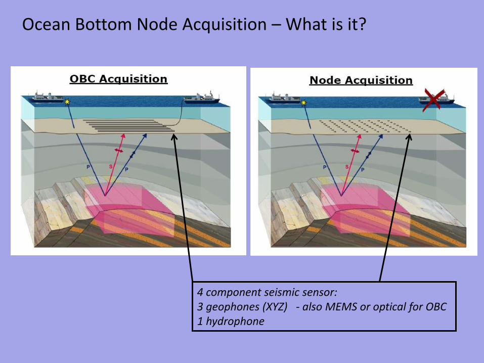
Ocean Bottom Node Acquisition – What is it?
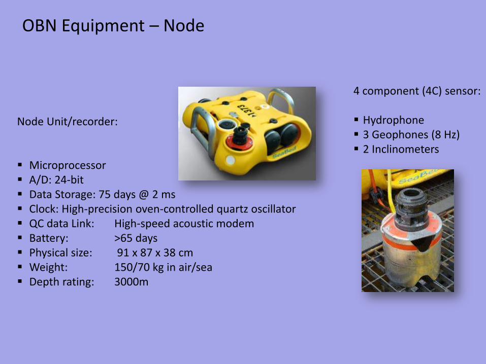
4 component seismic sensor: 3 geophones (XYZ) - also MEMS or optical for OBC 1 hydrophone
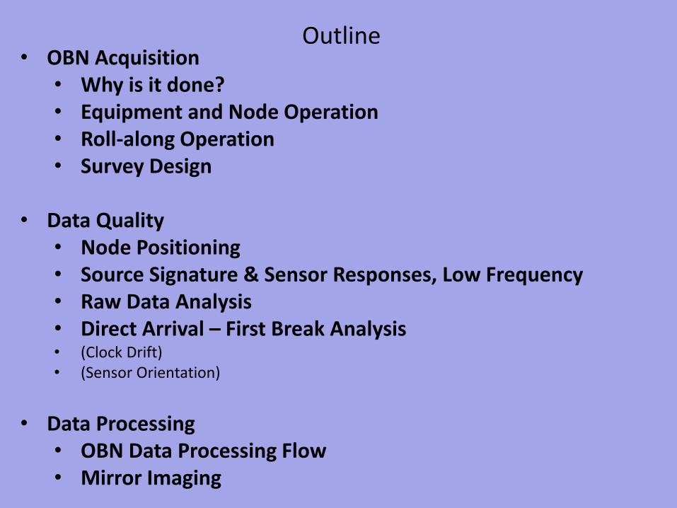
Outline • OBN Acquisition
• Why is it done? • Equipment and Node Operation • Roll-along Operation • Survey Design
• Data Quality
• Node Positioning • Source Signature & Sensor Responses, Low Frequency • Raw Data Analysis • Direct Arrival – First Break Analysis • (Clock Drift) • (Sensor Orientation)
• Data Processing
• OBN Data Processing Flow • Mirror Imaging
OBN Acquisition
Why is it done?
OBN Acquisition – Why is it done? Complex imaging with full azimuth broad band data
Source: Atlantis, Node data acquired by Fairfield (phase 1) & Seabird (phase 2)
Beaudoin SEG 2010
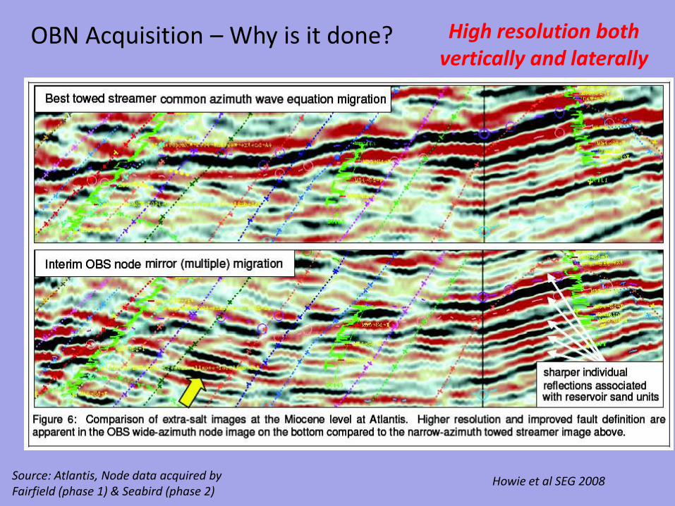
OBN Acquisition – Why is it done? High resolution both vertically and laterally
Howie et al SEG 2008 Source: Atlantis, Node data acquired by Fairfield (phase 1) & Seabird (phase 2)
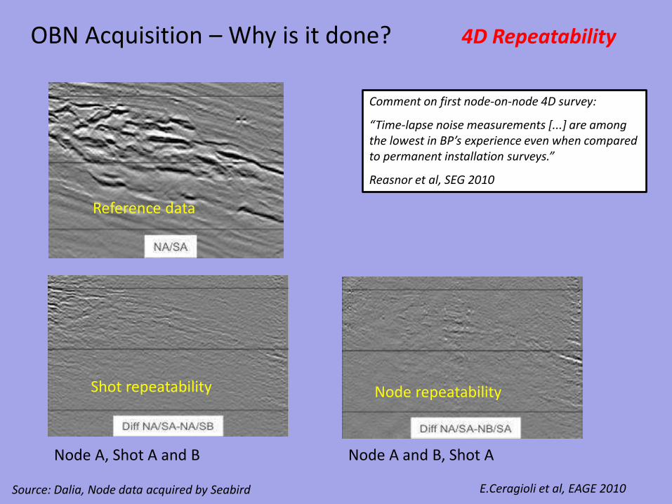
OBN Acquisition – Why is it done? 4D Repeatability
Reference data
Node A, Shot A and B Node A and B, Shot A
E.Ceragioli et al, EAGE 2010
Shot repeatability Node repeatability
Source: Dalia, Node data acquired by Seabird
Comment on first node-on-node 4D survey:
“Time-lapse noise measurements [...] are among the lowest in BP’s experience even when compared to permanent installation surveys.”
Reasnor et al, SEG 2010
OBN Acquisition – Why is it done? Infill under obstructions, congested oilfields
OBN Acquisition – Why is it done?
Beaudoin, SEG 2010
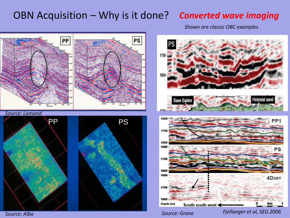
PP PS
Fjellanger et al, SEG 2006 Source: Alba
Source: Lomond
Source: Grane
Converted wave imaging Shown are classic OBC examples
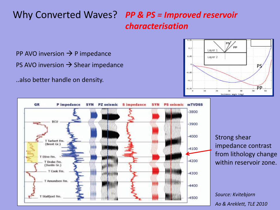
Strong shear impedance contrast from lithology change within reservoir zone.
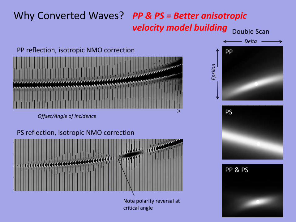
Why Converted Waves? PP & PS = Better anisotropic velocity model building
PP reflection, isotropic NMO correction
PS reflection, isotropic NMO correction
Double Scan
PP
PS
PP & PS
Epsi
lon
Delta
Note polarity reversal at critical angle
Offset/Angle of incidence
OBN Acquisition
Equipment and Node Operation
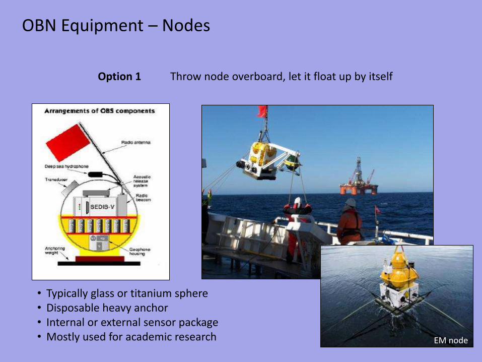
OBN Equipment – Nodes
Option 1 Throw node overboard, let it float up by itself
• Typically glass or titanium sphere • Disposable heavy anchor • Internal or external sensor package • Mostly used for academic research EM node
OBN Equipment – Nodes
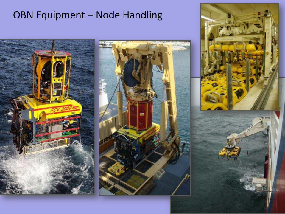
Option 2 Hand-place node, pick it up manually
• Node can be custom shaped • Recorder in cylindrical pressure vessels • Internal or external sensor package • Mostly used for commercial 3D surveys
OBN Equipment – Node
Node Unit/recorder: Microprocessor A/D: 24-bit Data Storage: 75 days @ 2 ms Clock: High-precision oven-controlled quartz oscillator QC data Link: High-speed acoustic modem Battery: >65 days Physical size: 91 x 87 x 38 cm Weight: 150/70 kg in air/sea Depth rating: 3000m
• Hydrophones need to be exposed to outside • Geophones need to couple to seabed (in order to
record shear waves)
• MEMS accelerometers or optical sensors are not suitable for autonomous nodes due to high power consumption of the sensor itself or of other system components
• Others, such as piezo-electric sensors are also an option
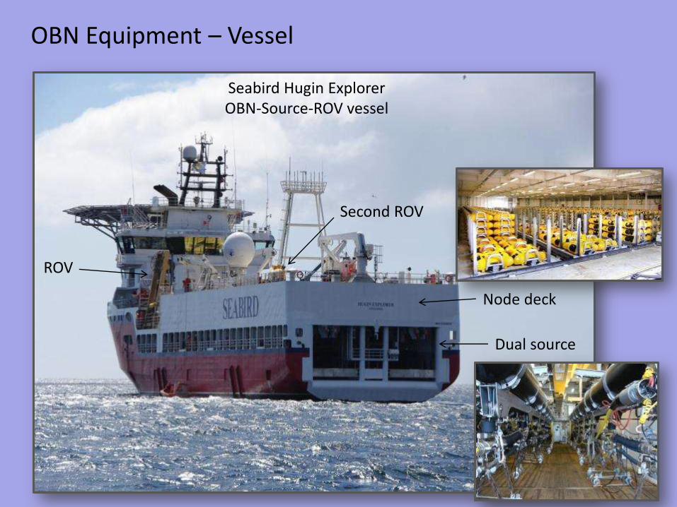
OBN Equipment – Vessel
Seabird Hugin Explorer OBN-Source-ROV vessel
ROV
Node deck
Dual source
Second ROV
OBN Equipment – Node Handling
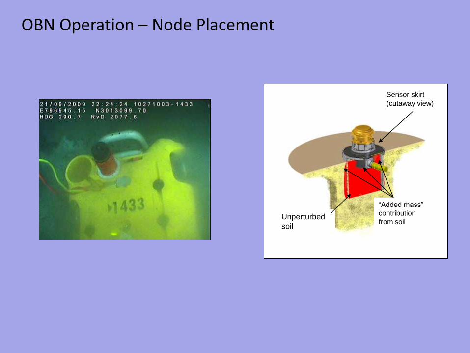
OBN Operation – Node Placement
OBN Operation – Node Placement
“Added mass”
contribution
from soil
Sensor skirt
(cutaway view)
Unperturbed
soil
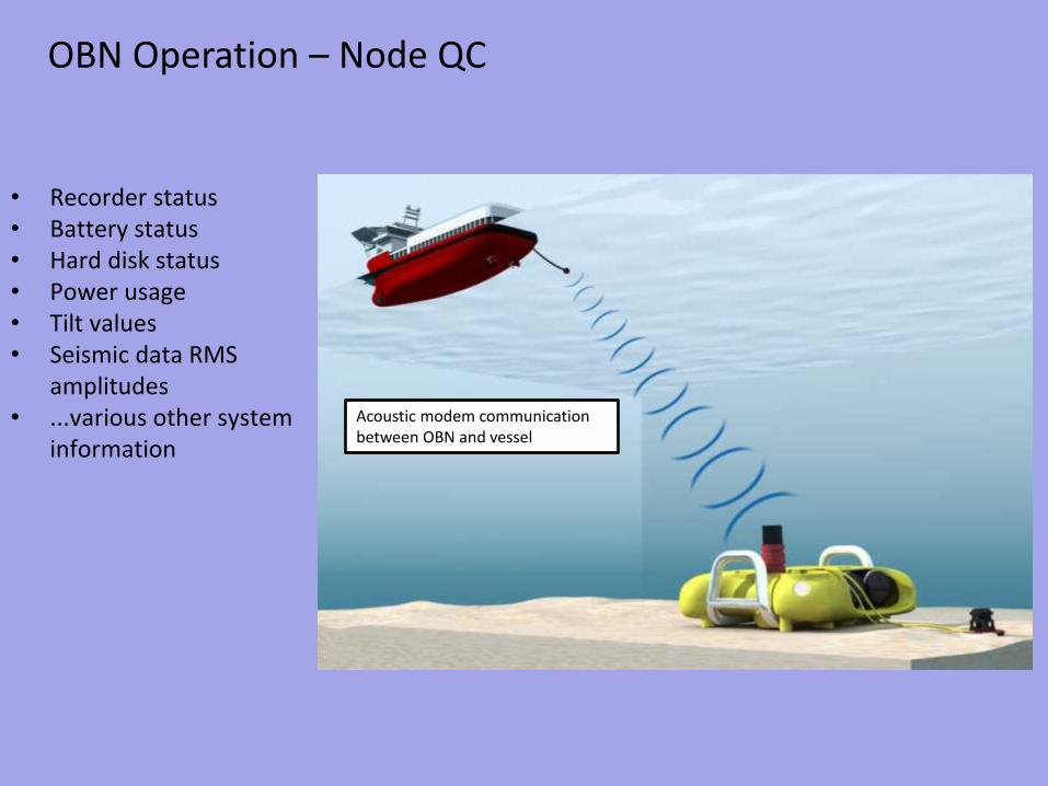
OBN Operation – Node QC
Acoustic modem communication between OBN and vessel
• Recorder status • Battery status • Hard disk status • Power usage • Tilt values • Seismic data RMS
amplitudes • ...various other system
information
OBN Acquisition
Roll-along Operation
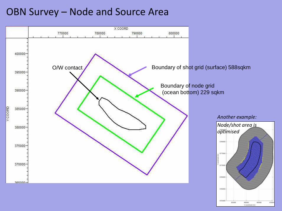
Boundary of shot grid (surface) 588sqkm
Boundary of node grid
(ocean bottom) 229 sqkm
O/W contact
OBN Survey – Node and Source Area
Another example:
Node/shot area is optimised
• 1595 total node positions • Node grid: 390m x 390m
OBN Survey – Node Layout
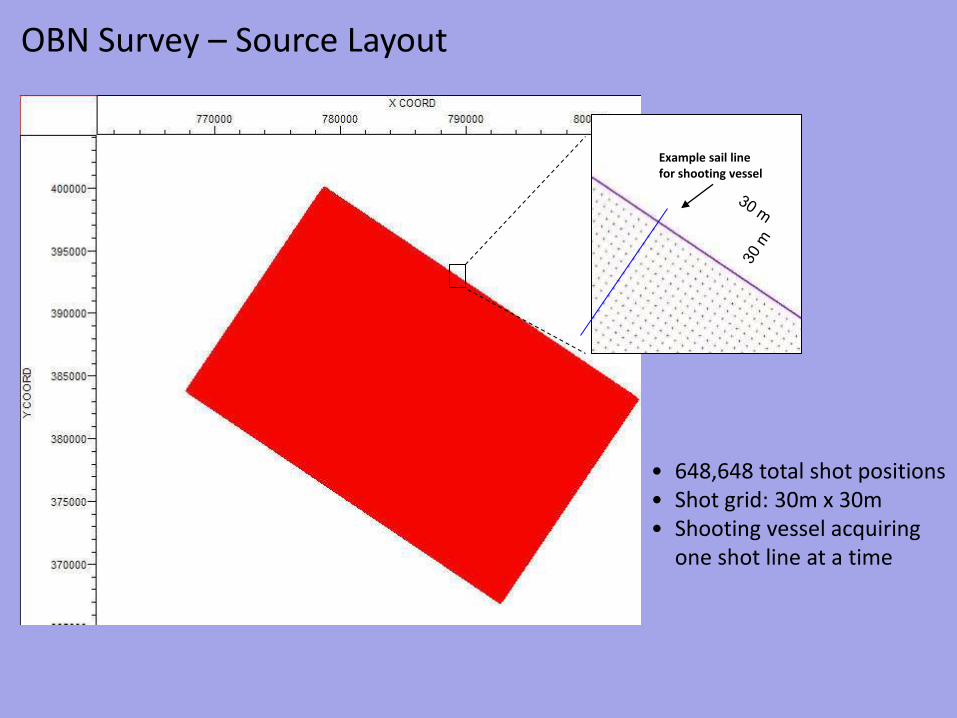
• 648,648 total shot positions • Shot grid: 30m x 30m • Shooting vessel acquiring
one shot line at a time
Example sail line for shooting vessel
OBN Survey – Source Layout
First node line
13-line shot swath
N
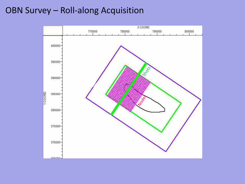
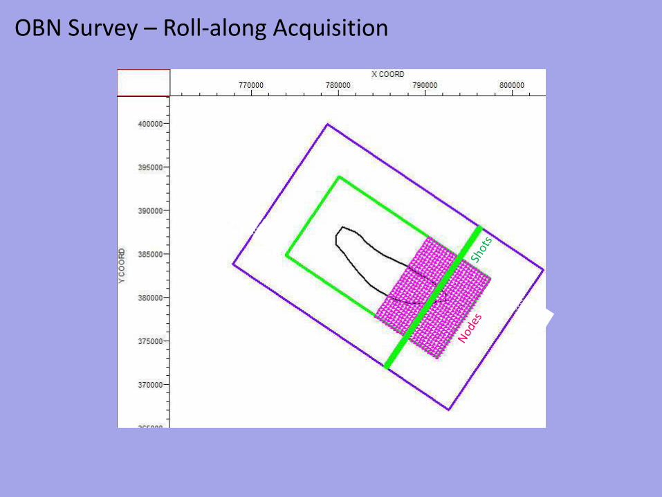
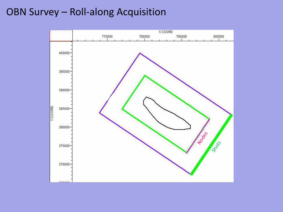
OBN Survey – Roll-along Acquisition
OBN Survey – Roll-along Acquisition
OBN Survey – Roll-along Acquisition
OBN Survey – Roll-along Acquisition
OBN Survey – Roll-along Acquisition
OBN Survey – Roll-along Acquisition
25th shot swath
OBN Survey – Roll-along Acquisition
OBN Survey – Roll-along Acquisition
OBN Survey – Roll-along Acquisition
OBN Acquisition
Survey Design
Area of interest
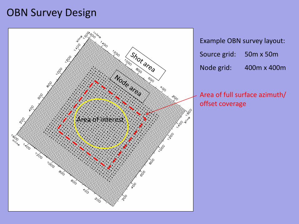
OBN Survey Design
Example OBN survey layout:
Source grid: 50m x 50m
Node grid: 400m x 400m
Area of full surface azimuth/ offset coverage
Area of interest
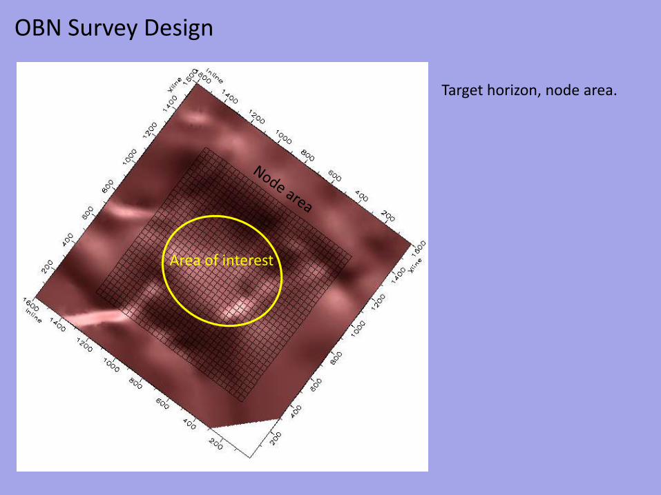
OBN Survey Design
Target horizon, node area.
Area of interest
OBN Survey Design
Ray-tracing, PP mode
OBN Survey Design
Ray-tracing, P-to-S conversion
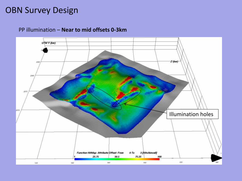
OBN Survey Design
PP illumination – Near to mid offsets 0-3km
Illumination holes
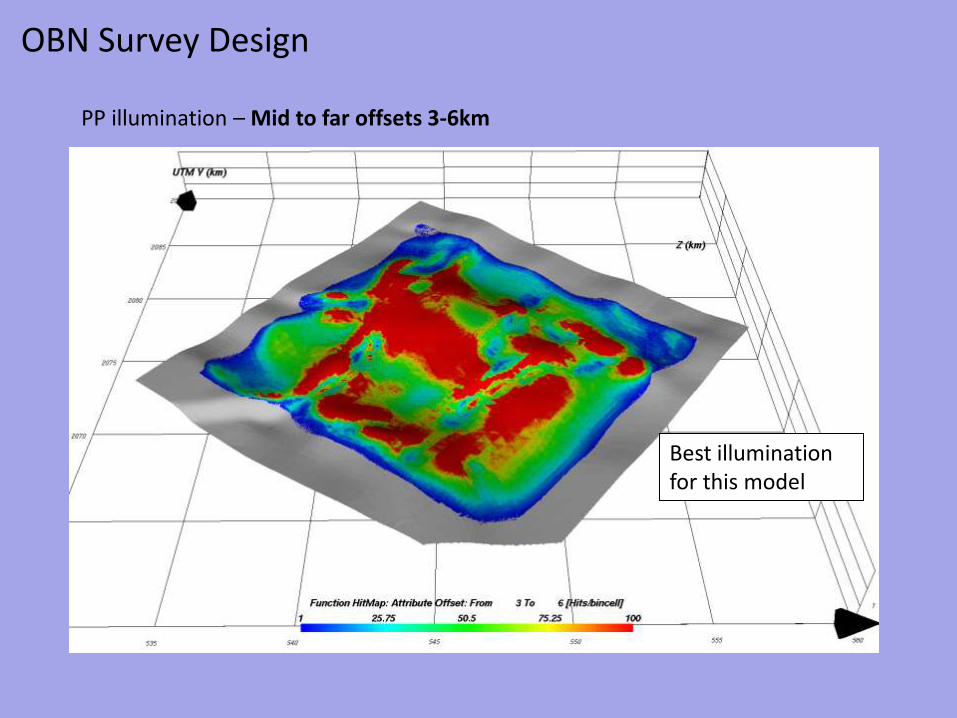
OBN Survey Design
PP illumination – Mid to far offsets 3-6km
Best illumination for this model
OBN Survey Design
PP illumination – Very far offsets 6-9km
OBN Survey Design
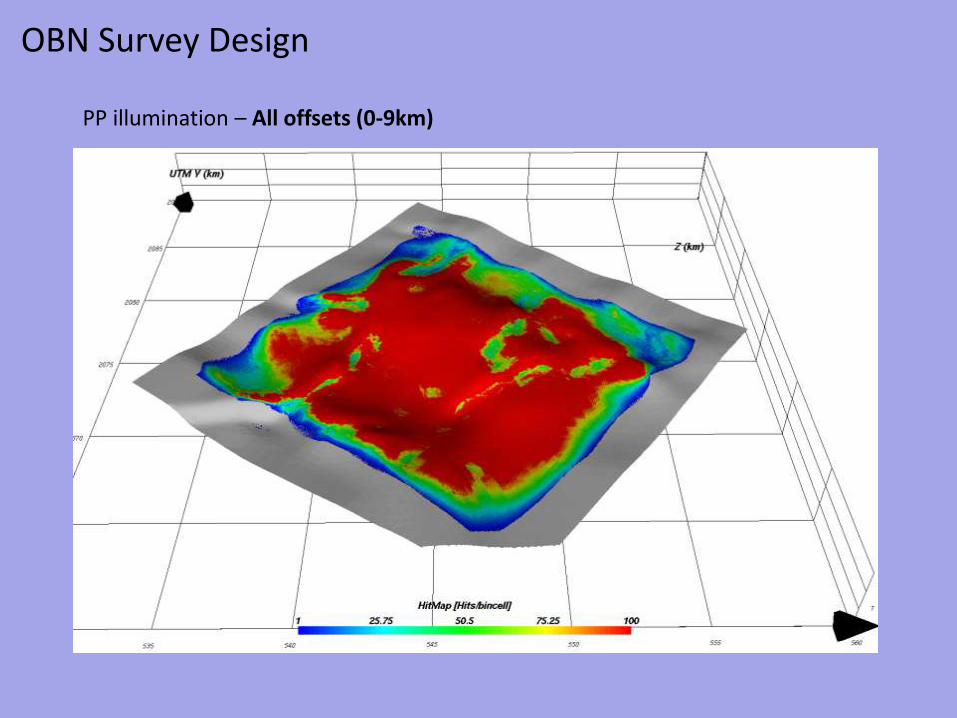
PP illumination – All offsets (0-9km)
OBN Survey Design
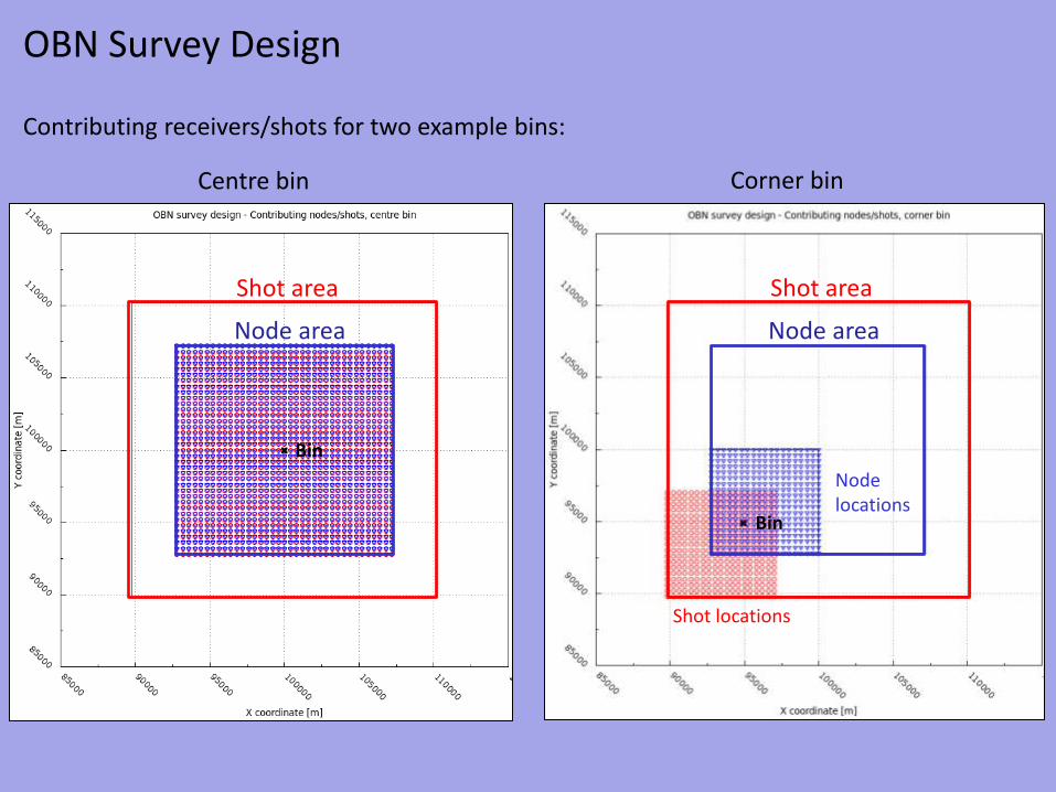
Node area
Shot area
Node area
Shot area
Contributing receivers/shots for two example bins:
Centre bin Corner bin
Node locations
Shot locations
Bin
Bin
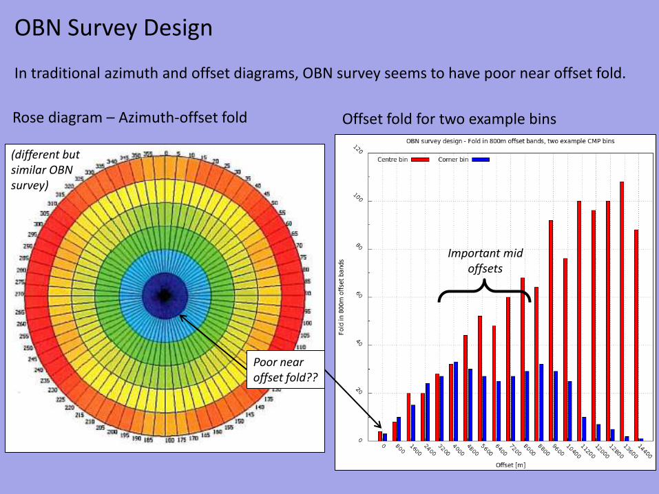
OBN Survey Design
Rose diagram – Azimuth-offset fold
In traditional azimuth and offset diagrams, OBN survey seems to have poor near offset fold.
(different but similar OBN survey)
Offset fold for two example bins
Important mid offsets
Poor near offset fold??
OBN Survey Design
OBN offset/azimuth fold is best viewed in so-called “common-offset vector tiles”. For any CMP bin, contributing shot-receiver pairs are evenly distributed on a regular offset/azimuth grid. Pre-stack migration is best performed in common offset vector tiles.
Within the limits of survey area, every bin has even contributions of all azimuths and offsets.
Centre bin Corner bin
Even offset distribution in every azimuth direction
OBN Acquisition
Node Positioning
Node Positioning – Systems
• USBL – Ultra Short Baseline
– Vessel based transceiver acoustically interrogates remote beacon to determine a range/bearing and computes relative position from vessel GPS. Average accuracy is a function of water depth/slant range.
• INS – Inertial Navigation System
– Comprised of Inertial Measurement Unit (IMU) and software Kalman filter. IMU senses motion and direction, with Kalman filter, to maintain accuracy away from control points.
• LBL – Long Baseline
– Comprised of an array of N transponder beacons placed at the seafloor which are calibrated in a relative manner. Unambiguous fix requires at least 3 ranges. Independent of depth.
– Costly and time consuming operation
Standard sub-sea positioning systems
Node Positioning – Systems
• HiPAP & SSBL
– High Precision Acoustic Positioning using Super Short Baseline
– Hull mounted unit & ROV transducers
• HAIN
– Hydro-acoustic Aided Inertial Navigation System
– Inertial Measurement Unit (3 gyro compasses & 3 accelerometers)
– Doppler Velocity Log (ROV speed)
– Pressure & heading sensor
– Kalman software filter
High-fidelity sub-sea positioning system
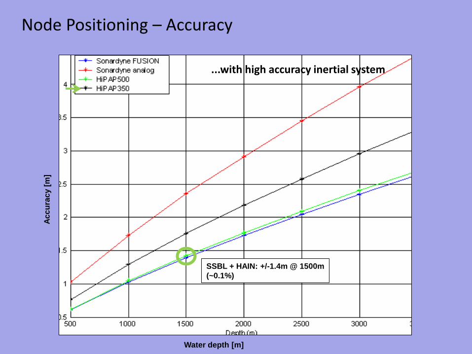
Node Positioning – Accuracy
SSBL: +/-6m @ 1500m
(~0.4%)
USBL: +/-12m @ 1500m
(~0.8%)
Water depth [m]
Ac
cu
rac
y [
m]
Node Positioning – Accuracy
SSBL + HAIN: +/-1.4m @ 1500m
(~0.1%)
...with high accuracy inertial system
Water depth [m]
Ac
cu
rac
y [
m]
Node Positioning – Accuracy
Real OBN survey #1: • 750 nodes • Water depth 1095m-1135m • Mean misplacement of
• 1.2m (real-time) • 1.9m (first break solution)
• 0.2% of water depth
Real-time position
...where we thought we were
Post-processing position
...where we really were
Node Positioning – Accuracy
Real OBN survey #2: • 1600 nodes • Water depth 1160m-1820m • Mean misplacement of
• 3.1m (real-time) • 3.3m (first break solution)
• 0.3% of water depth
Real-time position
...where we thought we were
Post-processing position
...where we really were
...intentionally placed far from preplot
OBN Acquisition
Source Signature & Sensor Responses
• What is put into the ground and what is recorded • How to boost low frequency energy to give broad band seismic
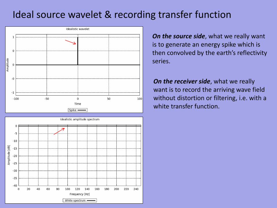
Ideal source wavelet & recording transfer function
On the source side, what we really want is to generate an energy spike which is then convolved by the earth’s reflectivity series.
On the receiver side, what we really want is to record the arriving wave field without distortion or filtering, i.e. with a white transfer function.
Real source signature
Real source wavelet • Band limited • Low frequency reverberations from
air bubble and source ghost
Real source spectrum • Band limited due to source output,
anti-alias filter and sensor reponse • Ripples at low end due to air bubble • Regularly spaced notches due to
surface source ghost
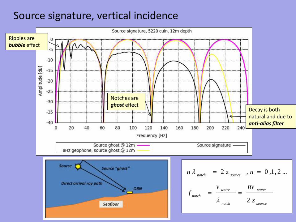
Source signature, vertical incidence
Ripples are bubble effect
Notches are ghost effect
Decay is both natural and due to anti-alias filter
source
water
notch
water
notch
sourcenotch
z
nvvf
nzn
2
...2,1,0,2
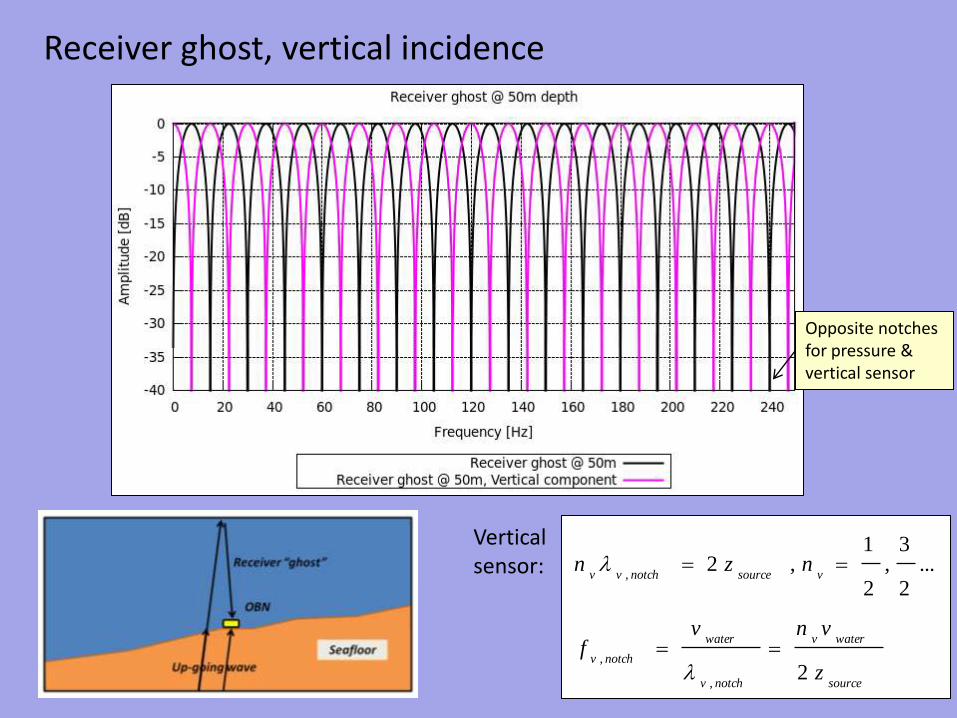
Receiver ghost, vertical incidence
Opposite notches for pressure & vertical sensor
source
waterv
notchv
water
notchv
vsourcenotchvv
z
vnvf
nzn
2
...2
3,
2
1,2
,
,
,
Vertical sensor:
Sensor response/source signature wavelet
8Hz geophone
8Hz geophone, anti-alias
8Hz geophone, anti-alias, source ghost @ 12m
8Hz geoph., anti-alias, example source signature @ 12m
In data processing we will try to compress the recorded seismic wavelet as much as possible, equivalent to flattening/whitening of the spectrum. • Care needs to be taken to avoid boosting noise in ghost notches
• De-bubble operator to remove bubble oscillations
• Full source de-signature operator
• Modelled versus data derived source signature wavelet
Source Signature Processing
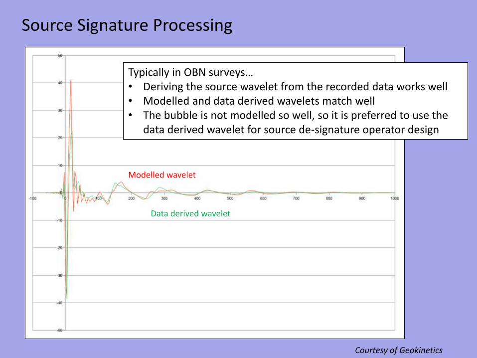
Modelled wavelet
Data derived wavelet
Typically in OBN surveys… • Deriving the source wavelet from the recorded data works well • Modelled and data derived wavelets match well • The bubble is not modelled so well, so it is preferred to use the
data derived wavelet for source de-signature operator design
Courtesy of Geokinetics
Source Signature Processing
Data derived source signature spectrum
Desired output spectrum after de-bubble operator
Courtesy of Geokinetics
Source Signature Processing
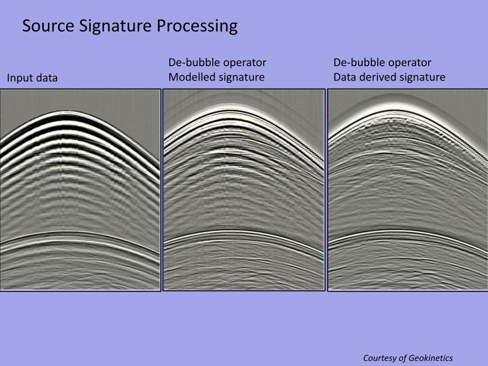
Courtesy of Geokinetics
Input data
De-bubble operator Modelled signature
De-bubble operator Data derived signature
Boosting low frequency energy
Why do we need low frequency information? • Improved resolution from broad band seismic • Deep, complex structural imaging, in particular:
‒ Sub-salt imaging ‒ Sub-basalt imaging ‒ Generally, penetrating high velocity layers and rugose interfaces
• Velocity model building • Inversion
Boosting low frequency energy (1)
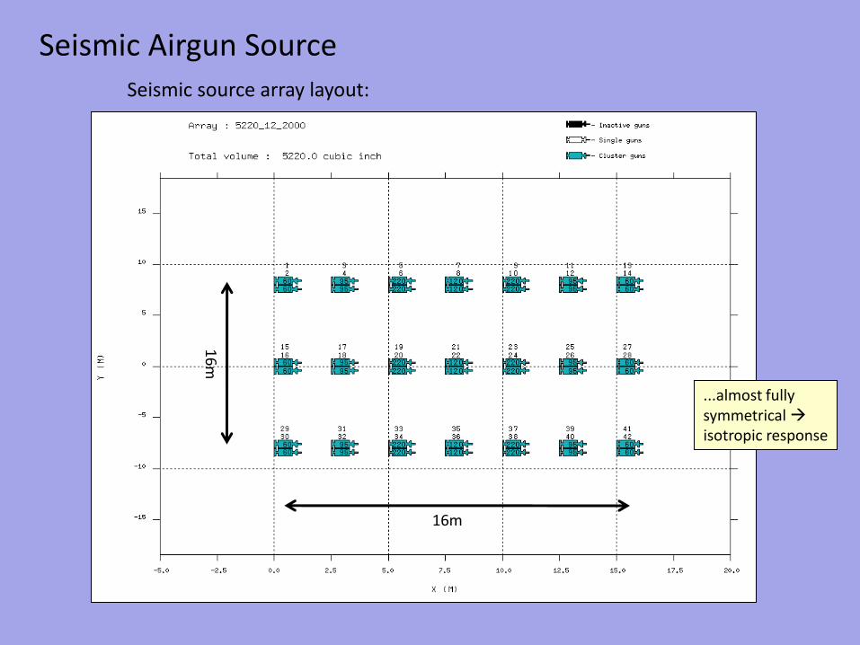
5000 cuin volume
4370 cuin volume
3dB @ 10Hz
Boost low frequency energy by… • …using a bigger source array
Downside • Limit to maximum source size, longer re-charge time, more shot generated noise
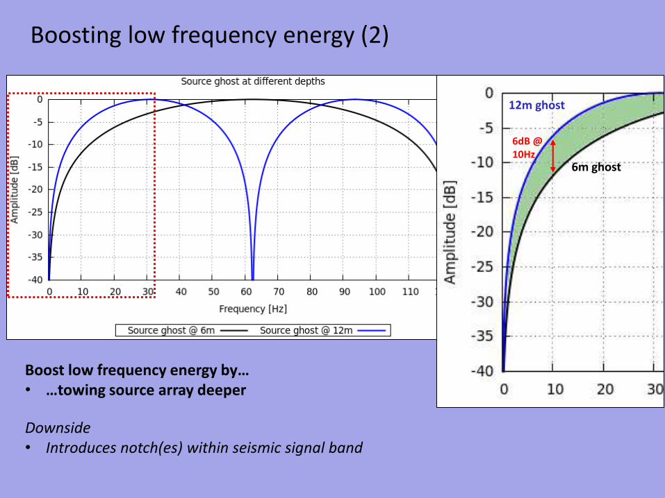
Boosting low frequency energy (2)
12m ghost
6m ghost
6dB @ 10Hz
Boost low frequency energy by… • …towing source array deeper
Downside • Introduces notch(es) within seismic signal band
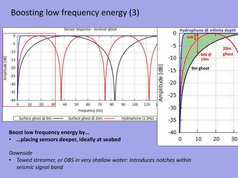
Boosting low frequency energy (3)
Hydrophone @ infinite depth
9m ghost
8dB @ 10Hz
Boost low frequency energy by… • …placing sensors deeper, ideally at seabed
Downside • Towed streamer, or OBS in very shallow water: Introduces notches within
seismic signal band
20m ghost
3dB
Boosting low frequency energy (4)
Boost low frequency energy by… • …performing de-ghosting / wavefield separation
Downside • Requires more costly acquisition:
Ocean bottom seismometers, over/under streamers, or others
Limited at low end only by • Sensor response • Sensor depth
Boosting low frequency energy (5)
8Hz geophone
14Hz geophone
5dB @ 10Hz
Boost low frequency energy by… • …using velocity sensors with high sensitivity and
wide dynamic range at low end
Downside • Low natural-frequency geophones are not omni-directional, i.e. they are sensitive to tilt
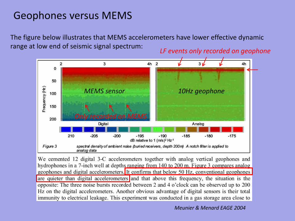
Geophones versus MEMS
Meunier & Menard EAGE 2004
MEMS sensor 10Hz geophone
LF events only recorded on geophone
Only recorded on MEMS
The figure below illustrates that MEMS accelerometers have lower effective dynamic range at low end of seismic signal spectrum:
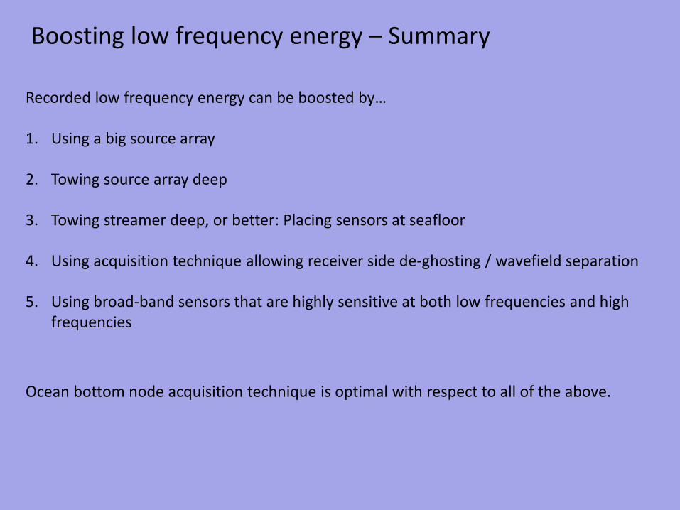
Boosting low frequency energy – Summary
Recorded low frequency energy can be boosted by… 1. Using a big source array
2. Towing source array deep
3. Towing streamer deep, or better: Placing sensors at seafloor
4. Using acquisition technique allowing receiver side de-ghosting / wavefield separation
5. Using broad-band sensors that are highly sensitive at both low frequencies and high
frequencies
Ocean bottom node acquisition technique is optimal with respect to all of the above.
OBN Acquisition
Raw Data Analysis
Continuous recorded data
Active shooting DC shift
• Active shots need to be extracted from continuous record, using shot time
• Shot time needs to be mapped to time of internal clock
• Clocks used in OBNs are very accurate, but still drift by several 10ms per month
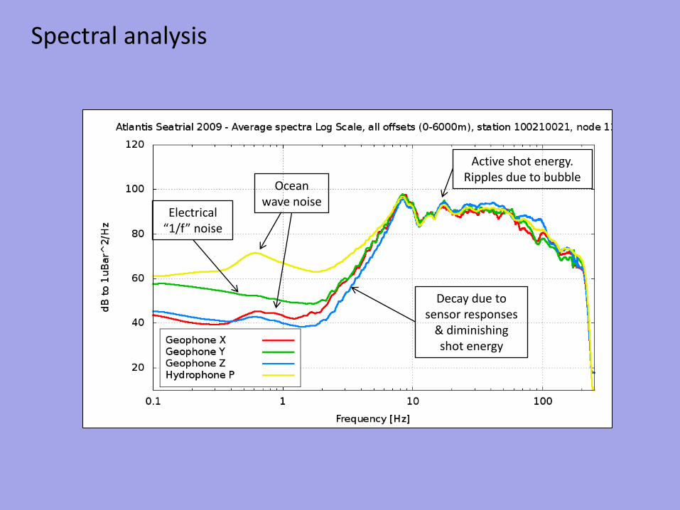
Spectral analysis
Electrical “1/f” noise
Ocean wave noise
Decay due to sensor responses
& diminishing shot energy
Active shot energy. Ripples due to bubble
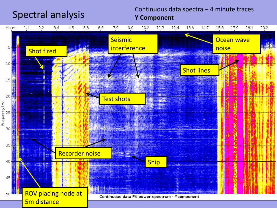
Spectral analysis
Shot lines
Shot fired
Recorder noise
Ocean wave noise
ROV placing node at 5m distance
Seismic interference
Test shots
1
2
3 4
5
6
7
8
Ship
Continuous data spectra – 4 minute traces X Component
Spectral analysis
Test shots
Seismic interference Shot fired
Recorder noise
Shot lines
Ocean wave noise
ROV placing node at 5m distance
Ship
Continuous data spectra – 4 minute traces Y Component
Spectral analysis
Test shots
Seismic interference Shot fired
Recorder noise
ROV hoisted on deck
Shot lines
Ocean wave noise
ROV placing node at 5m distance
Ship
Continuous data spectra – 4 minute traces Z Component
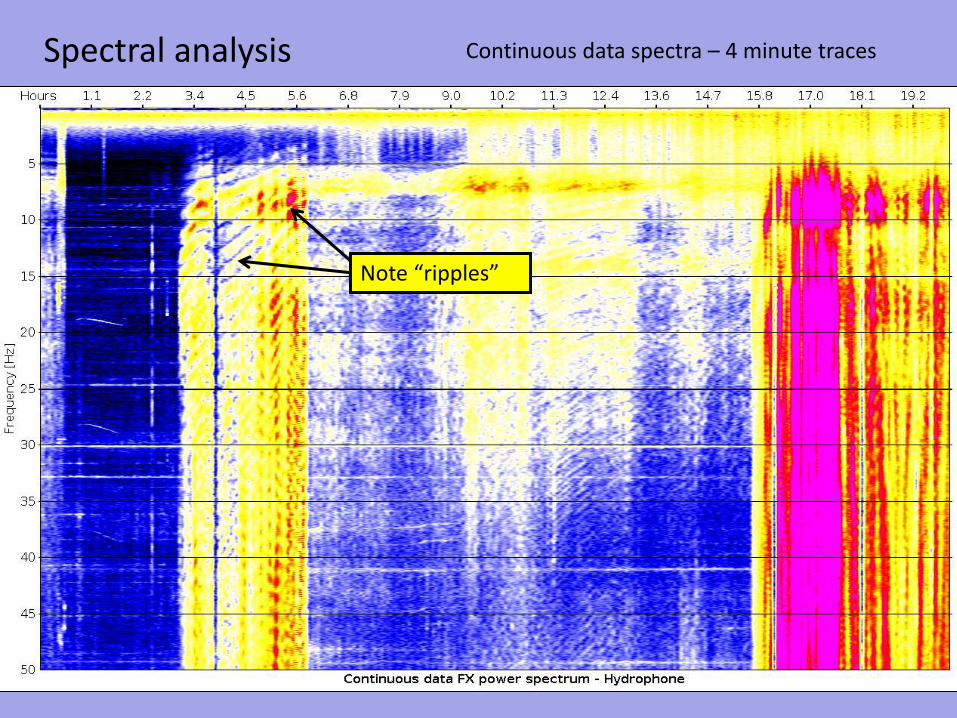
Spectral analysis
Test shots
Seismic interference Shot fired
Recorder noise
ROV hoisted on deck
Ocean wave noise
Shot lines
Ship
Continuous data spectra – 4 minute traces Hydrophone
Spectral analysis
5 hours of recording 5 hours of recording
Earthquake/ Seaslide
Same spectrum, zoomed in 0-0.7Hz
Continuous data spectra – 4 minute traces Hydrophone
Spectral analysis
Note “ripples”
Continuous data spectra – 4 minute traces
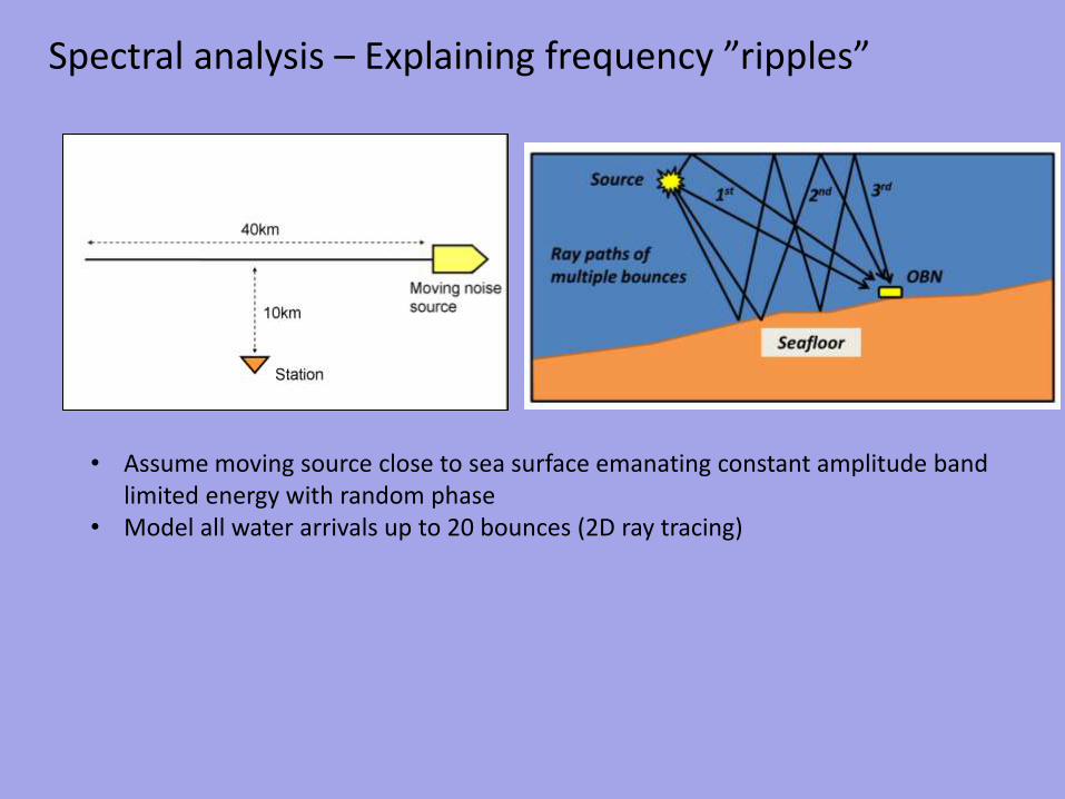
Spectral analysis – Explaining frequency ”ripples”
• Assume moving source close to sea surface emanating constant amplitude band limited energy with random phase
• Model all water arrivals up to 20 bounces (2D ray tracing)
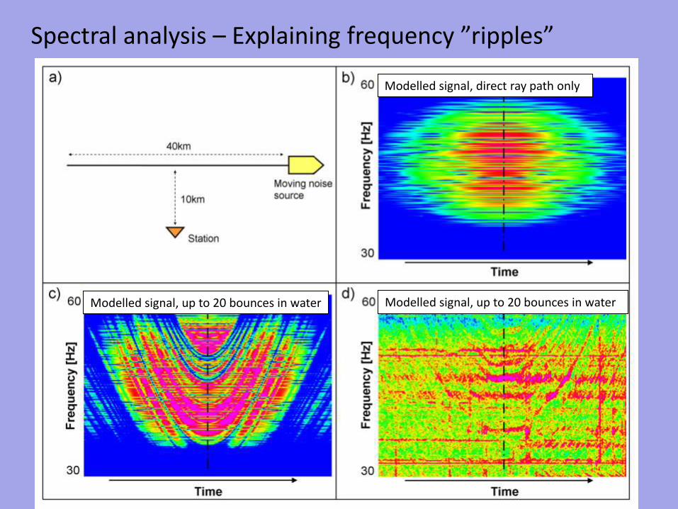
Spectral analysis – Explaining frequency ”ripples”
Modelled signal, direct ray path only
Modelled signal, up to 20 bounces in water Modelled signal, up to 20 bounces in water
X Y Z Hydrophone
Example raw receiver gather, deep water (~1km)
First water
bottom multiple
Direct arrival
Second?
Shear noise
“Zero“ offset
Raw data analysis
P-wave
reflection
PS
converted
waves
Bubble
2D node gather from one shot line, displayed with true relative amplitude and constant water velocity NMO correction.
Node position Node position
Seafloor mirror image (first water bottom multiple)
Usages for recorded direct arrival wave = Parameters that can be derived from first break pick times:
Direct arrival – First break times
td
t
tzv
zyx
zyx
tdttzv
zzyyxxt
sss
rrr
srsrsr
0
0
,
,,
,,
,
1
: Receiver/Node position
: Source position
: Average water velocity (at best function of depth and time)
: Residual time shift
: Clock drift (time variant)
Direct arrival travel time equation:
Assumptions: • Straight ray path • No global position biases • First break pick represents true travel time • ...
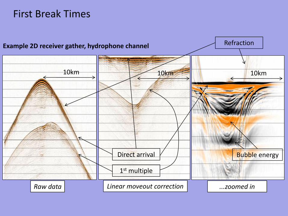
First Break Times
Raw data
Example 2D receiver gather, hydrophone channel
Linear moveout correction ...zoomed in
10km 10km 10km
Refraction
1st multiple
Direct arrival Bubble energy
Fictitious node survey
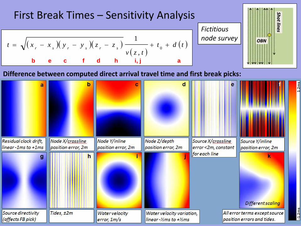
Difference between computed direct arrival travel time and first break picks:
First Break Times – Sensitivity Analysis
tdttzv
zzyyxxtsrsrsr
0
,
1
b c a d e f i, j h
Water velocity
Water velocity profiles taken over the same area at different times and locations:
750m
1500m
...illustrates that in general, water velocity is invariant neither in space nor in time.
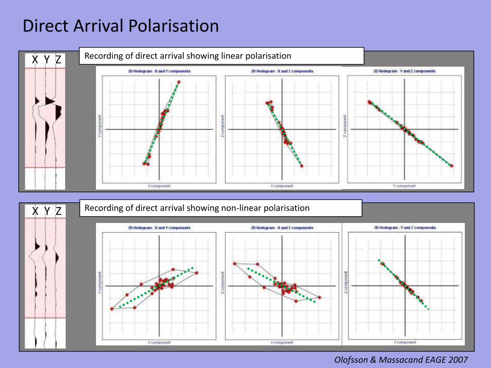
Recording of direct arrival showing non-linear polarisation X Y Z
XY XZ YZ
X Y Z
Recording of direct arrival showing linear polarisation X Y Z
XY XZ YZ
X Y Z
Direct Arrival Polarisation
Olofsson & Massacand EAGE 2007
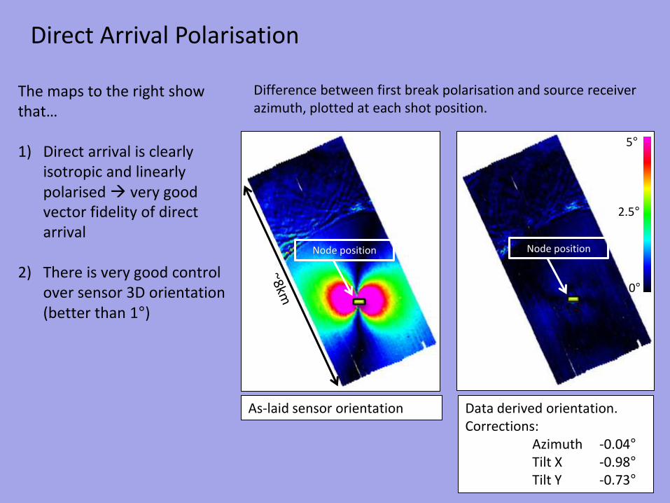
Direct Arrival Polarisation
Difference between first break polarisation and source receiver azimuth, plotted at each shot position.
5°
0°
2.5°
As-laid sensor orientation Data derived orientation. Corrections: Azimuth -0.04° Tilt X -0.98° Tilt Y -0.73°
The maps to the right show that… 1) Direct arrival is clearly
isotropic and linearly polarised very good vector fidelity of direct arrival
2) There is very good control over sensor 3D orientation (better than 1°)
Node position Node position
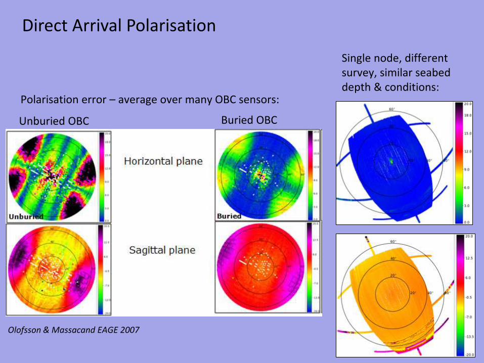
Direct Arrival Polarisation
Unburied OBC
Olofsson & Massacand EAGE 2007
Buried OBC
Single node, different survey, similar seabed depth & conditions:
Polarisation error – average over many OBC sensors:
OBN Acquisition
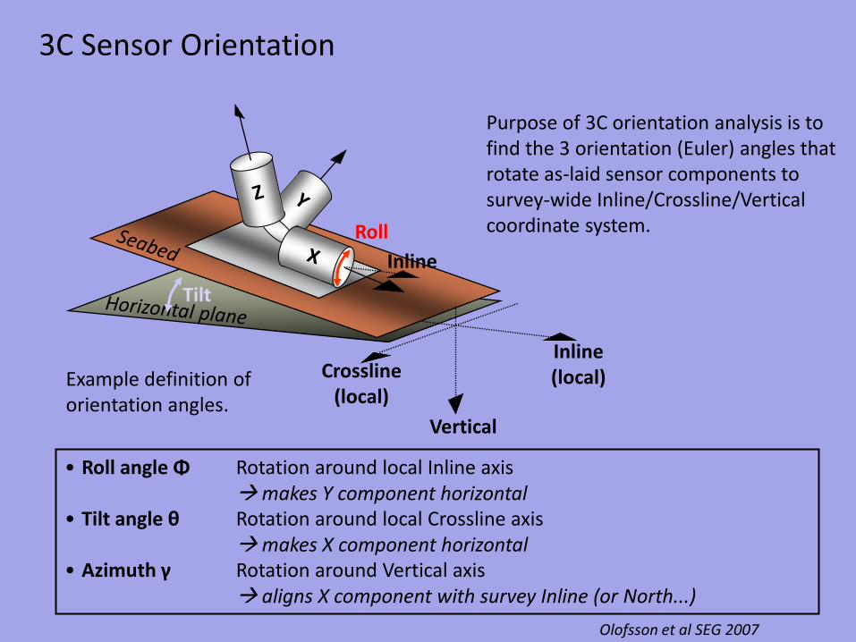
3C Sensor Orientation
Inline (local)
Vertical
Crossline (local)
Inline
Tilt
Roll
• Roll angle Φ Rotation around local Inline axis makes Y component horizontal
• Tilt angle θ Rotation around local Crossline axis makes X component horizontal
• Azimuth γ Rotation around Vertical axis aligns X component with survey Inline (or North...)
Purpose of 3C orientation analysis is to find the 3 orientation (Euler) angles that rotate as-laid sensor components to survey-wide Inline/Crossline/Vertical coordinate system.
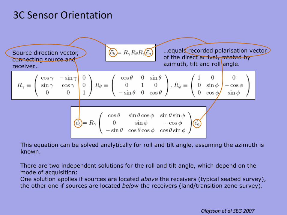
3C Sensor Orientation
Example definition of orientation angles.
Olofsson et al SEG 2007
This equation can be solved analytically for roll and tilt angle, assuming the azimuth is known.
Source direction vector, connecting source and receiver…
…equals recorded polarisation vector of the direct arrival, rotated by azimuth, tilt and roll angle.
There are two independent solutions for the roll and tilt angle, which depend on the mode of acquisition: One solution applies if sources are located above the receivers (typical seabed survey), the other one if sources are located below the receivers (land/transition zone survey).
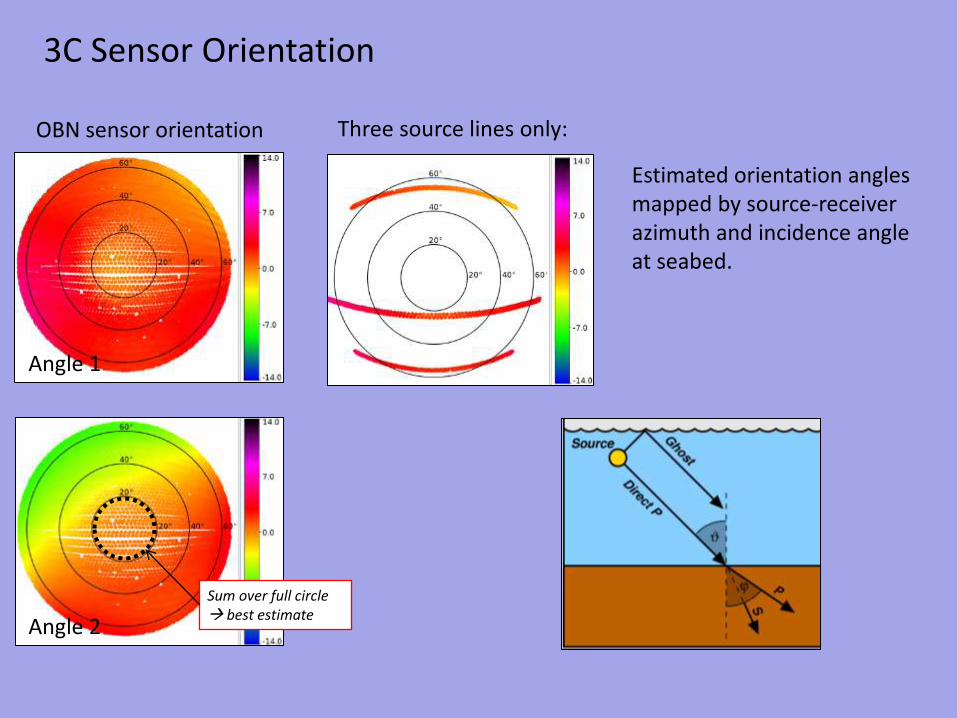
3C Sensor Orientation
Olofsson et al SEG 2007
OBN sensor orientation
Angle 1
Angle 2
3C Sensor Orientation
Sum over full circle best estimate
Three source lines only:
Estimated orientation angles mapped by source-receiver azimuth and incidence angle at seabed.
Buried OBC Unburied OBC
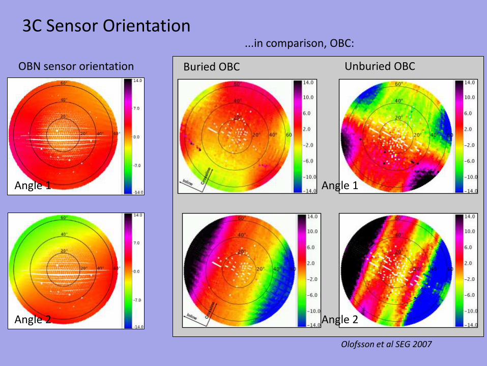
3C Sensor Orientation
OBN sensor orientation
Angle 1
Angle 2
...in comparison, OBC:
Angle 1
Angle 2
Olofsson et al SEG 2007
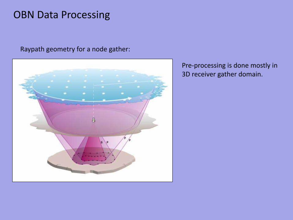
OBN Data Processing
OBN Data Processing
Raypath geometry for a node gather:
Pre-processing is done mostly in 3D receiver gather domain.
SEGY input
Noise attenuation/ despike
PZ calibration (Z-to-P)
Source designature/ debubble
Vz noise attenuation
Geophone Hydrophone
Source designature/ debubble
Wavefield separation/ PZ combination
Upgoing Downgoing
up/down decon
Noise attenuation Noise attenuation
TTI PSDM TTI mirror PSDM
Radon demultiple Radon demultiple
stack stack
post-stack processing
post-stack processing
SRME demultiple
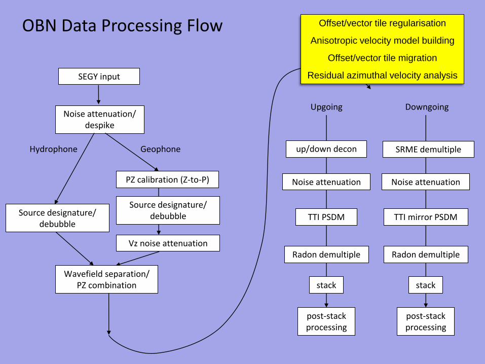
OBN Data Processing Flow
SEGY input
Noise attenuation/ despike
PZ calibration (Z-to-P)
Source designature/ debubble
Vz noise attenuation
Geophone Hydrophone
Source designature/ debubble
Wavefield separation/ PZ combination
Upgoing Downgoing
up/down decon
Noise attenuation Noise attenuation
TTI PSDM TTI mirror PSDM
Radon demultiple Radon demultiple
stack stack
post-stack processing
post-stack processing
SRME demultiple
OBN Data Processing Flow Offset/vector tile regularisation
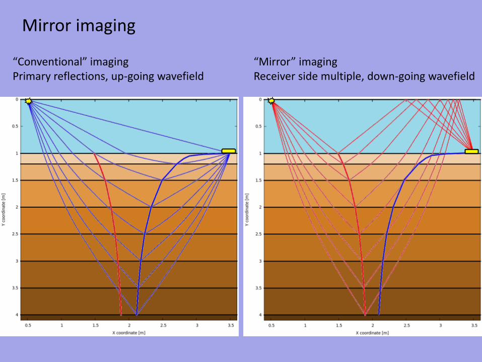
“Mirror” imaging Receiver side multiple, down-going wavefield
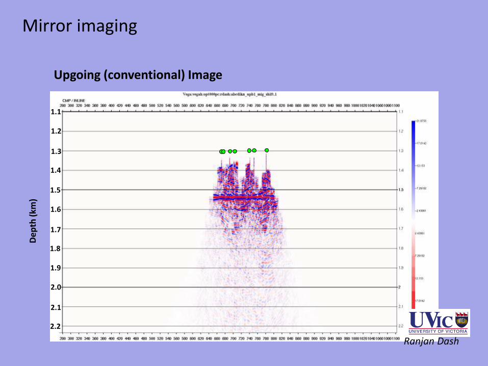
Mirror imaging
1.1
1.2
1.3
1.4
1.5
1.6
1.7
1.8
1.9
2.0
2.1
2.2
De
pth
(km
)
Ranjan Dash
Upgoing (conventional) Image
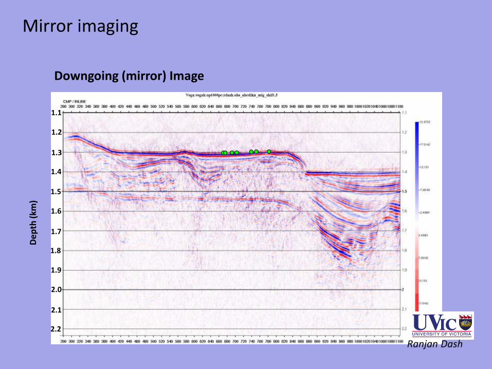
Mirror imaging
1.1
1.2
1.3
1.4
1.5
1.6
1.7
1.8
1.9
2.0
2.1
2.2
De
pth
(km
)
Ranjan Dash
Downgoing (mirror) Image
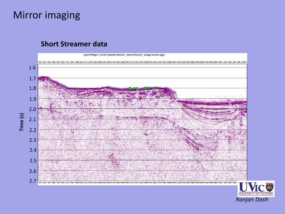
Mirror imaging Ti
me
(s)
1.6
1.7
1.8
1.9
2.0
2.1
2.2
2.3
2.4
2.5
2.6
2.7
Ranjan Dash
Short Streamer data
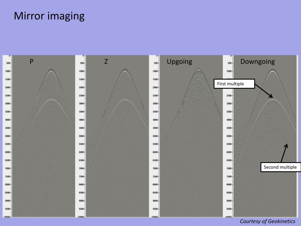
Mirror imaging
P Z Upgoing Downgoing
First multiple
Second multiple
Courtesy of Geokinetics
Mirror imaging
P Z
Downgoing Upgoing
After PZ calibration, debubble operator, Vz noise attenuation and PZ combination.
Example – Raw input data
Courtesy of Geokinetics
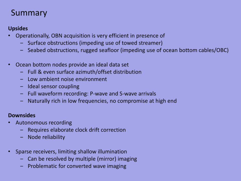
Summary
Upsides • Operationally, OBN acquisition is very efficient in presence of
‒ Surface obstructions (impeding use of towed streamer) ‒ Seabed obstructions, rugged seafloor (impeding use of ocean bottom cables/OBC)
• Ocean bottom nodes provide an ideal data set
‒ Full & even surface azimuth/offset distribution ‒ Low ambient noise environment ‒ Ideal sensor coupling ‒ Full waveform recording: P-wave and S-wave arrivals ‒ Naturally rich in low frequencies, no compromise at high end
‒ Can be resolved by multiple (mirror) imaging ‒ Problematic for converted wave imaging
References
Seismic noise without a seismic source, J. Meunier, J.Menard, EAGE, Extended Abstracts H022, (2004) Ocean Bottom Nodes Processing: reconciliation of Streamer and OBN data sets for Time Lapse Seismic Monitoring. The Angolan Deep Offshore Experience, Loïc Bovet, Enrico Ceragioli, Sergio Tchikanha, Jérôme Guilbot and Sylvain Toinet, SEG, Expanded Abstracts, 29 , no. 1, 3751-3755, (2010) Imaging the invisible — BP's path to OBS nodes, Gerard Beaudoin, SEG, Expanded Abstracts, 29 , no. 1, 3734-3739, (2010) Unlocking the full potential of Atlantis with OBS nodes, John Howie, Patrice Mahob, David Shepherd and Gerard Beaudoin, SEG, Expanded Abstracts, 27 , no. 1, 363-367, (2008) The Dalia OBN Project, E. Ceragioli (Total E&P Angola), L. Bovet (Total E&P Angola), J. Guilbot (Total E&P Angola) & S. Toinet (Total E&P Angola), EAGE, Extended Abstracts (2010) Successful use of converted wave data for interpretation and well optimization on Grane, Fjellanger J.P., Boen F., Ronning K.J./Hydro Oil & Energy, SEG, Expanded Abstracts (2006) Polarisation analysis of ocean bottom 3C sensor data, Bjorn Olofsson & Christophe Massacand, EAGE, Extended Abstracts (2007) Structural interpretation using PS seismic on the Kvitebjørn Field in the North Sea, Chau Ao and Edel K. Areklett, The Leading Edge 29, 402-407 (2010)