119
Trausti Hannesson Seismic Analysis and Design of a Concrete Arch Bridge Direct Displacement-based Design Approach to Seismic Isolation Master’s Thesis, April 2010

Trausti Hannesson
Seismic Analysis and Design of aConcrete Arch Bridge
Direct Displacement-based Design Approach toSeismic Isolation
Master’s Thesis, April 2010


Trausti Hannesson
Seismic Analysis and Design of aConcrete Arch Bridge
Direct Displacement-based Design Approach toSeismic Isolation
Master’s Thesis, April 2010


Seismic Analysis and Design of a Concrete Arch Bridge, Direct Displacement-basedDesign Approach to Seismic Isolation
This report was prepared byTrausti Hannesson
SupervisorsChristos Georgakis, Technical University of DenmarkBjarni Bessason, University of Iceland
Release date: April 2010Category: 1 (public)
Edition: First
Comments: This report is part of the requirements to achieve the Master ofScience in Engineering (M.Sc.Eng.) at the Technical Universityof Denmark. This report represents 30 ECTS points.
Rights: ©Trausti Hannesson, 2010
Department of Civil EngineeringTechnical University of DenmarkBrovej building 118DK-2800 Kgs. LyngbyDenmark
www.byg.dtu.dkTel: (+45) 45 25 17 00E-mail: [email protected]


Preface
The work presented here is part of the requirements to achieve the Masterof Science in Engineering (M.Sc.Eng.) at the Department of Civil Engi-neering at the Technical University of Denmark. This report represents 30ECTS points. The work was performed at the Faculty of Engineering at theUniversity of Iceland.
I am grateful to my supervisor professor Bjarni Bessason at the Universityof Iceland for his guidance, ideas and encouragement during my thesis work.I would also like to thank professor Christos Georgakis at the Technical Uni-versity of Denmark for his comments and for giving me the opportunity todo my studies in Iceland. Finally I would like to thank Helgi Valdimarsson,Managing Director at Almenna Consulting Engineers for providing me witha working space during my thesis work.
Akureyri, April 2010
Trausti Hannesson [s080012]


Abstract
In this thesis the response of a concrete arch bridge to seismic loads corre-sponding to the South Iceland Seismic Zone (SISZ) is calculated. The an-alyzed bridge was originally designed for non-seismic load conditions. TheSouth Iceland Seismic Zone is an active seismic zone and several times sincethe settlement of Iceland structures have collapsed and casualties been re-ported in earthquakes in that area.
The main objective of this thesis is to evaluate the effect of changing thebridge location and come up with a suitable design alternative. Linear re-sponse spectrum analysis is performed with the general purpose FE-programSAP2000 from which it is clear that the bridge is in need of redesign towithstand the seismic loads occurring in the South Iceland Seismic Zone.
A direct displacement-based design approach is employed to design an isola-tion system using lead rubber bearings. Linear response spectrum analysisis performed using equivalent linear stiffness and damping to model the non-linear behavior of the base isolation. The nonlinear behavior of the isolationsystem was then further investigated with nonlinear time history analysisusing artificial ground motions.
The study shows that by introducing lead rubber bearings as the only changeto the original design the response to seismic loads can be significantly im-proved. The direct displacement-based design approach to the design ofseismically isolated structures proved to be simple and to offer control ofthe total structural response. Simple hand calculations were verified bylinear response spectrum analysis but considerable difference was observedbetween the linear and nonlinear methods in terms of expected displacementof the bridge deck and hence section forces. Results from response spectrumanalysis were in all cases conservative.
Keywords: seismic engineering, bridge engineering, direct displacement-based de-sign, seismic isolation, lead rubber bearings


Contents
List of Figures viii
List of Tables xii
Nomenclature xiv
1 Introduction 1
1.1 Background . . . . . . . . . . . . . . . . . . . . . . . . . . . . 1
1.2 Objectives . . . . . . . . . . . . . . . . . . . . . . . . . . . . . 4
2 Theory 5
2.1 Equations of Motion . . . . . . . . . . . . . . . . . . . . . . . 5
2.1.1 Single Degree of Freedom . . . . . . . . . . . . . . . . 5
2.1.2 Multiple Degrees of Freedom . . . . . . . . . . . . . . 6
2.2 Definition of Seismic Load . . . . . . . . . . . . . . . . . . . . 7
2.2.1 Time Histories . . . . . . . . . . . . . . . . . . . . . . 7
2.2.2 Response Spectrum . . . . . . . . . . . . . . . . . . . 8
2.3 Seismic Isolation . . . . . . . . . . . . . . . . . . . . . . . . . 9
2.3.1 Lead Rubber Bearings . . . . . . . . . . . . . . . . . . 10
2.3.1.1 Equivalent Linear Model . . . . . . . . . . . 13
2.4 Performance Based Design . . . . . . . . . . . . . . . . . . . . 15

2.4.1 Direct Displacement-Based Design . . . . . . . . . . . 17
2.4.1.1 Design Displacement . . . . . . . . . . . . . 18
2.4.1.2 Fundamentals . . . . . . . . . . . . . . . . . 19
2.4.1.3 Elastic Stiffness of Cracked Concrete Sections 20
2.4.1.4 Displacement-Based Design of Isolated Bridges 22
2.4.1.5 Comparison With Force-based Design Ap-proach . . . . . . . . . . . . . . . . . . . . . 28
2.5 Methods of Analysis . . . . . . . . . . . . . . . . . . . . . . . 29
2.5.1 Response Spectrum Analysis . . . . . . . . . . . . . . 30
2.5.2 Nonlinear Time History Analysis . . . . . . . . . . . . 32
2.6 Eurocode 8 . . . . . . . . . . . . . . . . . . . . . . . . . . . . 34
2.7 Ultimate Strength of Elements . . . . . . . . . . . . . . . . . 36
2.7.1 The Arch . . . . . . . . . . . . . . . . . . . . . . . . . 37
2.7.2 Shear Capacity . . . . . . . . . . . . . . . . . . . . . . 38
2.7.3 Piers and Spandrel Columns . . . . . . . . . . . . . . 38
2.7.4 Bridge Deck . . . . . . . . . . . . . . . . . . . . . . . . 39
3 The Bridge and Applied Load 41
3.1 The Bridge . . . . . . . . . . . . . . . . . . . . . . . . . . . . 41
3.1.1 Structural Elements . . . . . . . . . . . . . . . . . . . 42
3.1.2 Material Properties . . . . . . . . . . . . . . . . . . . . 43
3.1.3 Isolation Devices . . . . . . . . . . . . . . . . . . . . . 44
3.1.4 Modal Analysis . . . . . . . . . . . . . . . . . . . . . . 45
3.2 Applied Load . . . . . . . . . . . . . . . . . . . . . . . . . . . 48
3.2.1 Dead Load . . . . . . . . . . . . . . . . . . . . . . . . 48
3.2.2 Traffic Loads . . . . . . . . . . . . . . . . . . . . . . . 48
3.2.3 Temperature Load . . . . . . . . . . . . . . . . . . . . 51
3.2.4 Seismic Load . . . . . . . . . . . . . . . . . . . . . . . 52
3.2.4.1 The Design Response Spectrum . . . . . . . 52
3.2.4.2 Time Histories . . . . . . . . . . . . . . . . . 55

vii
3.2.5 Load Combinations . . . . . . . . . . . . . . . . . . . 57
4 Static and Linear Dynamic Analysis 59
4.1 Computational Model . . . . . . . . . . . . . . . . . . . . . . 59
4.2 Original Bridge . . . . . . . . . . . . . . . . . . . . . . . . . . 60
4.2.1 Response to Static Loads . . . . . . . . . . . . . . . . 60
4.2.2 Response to Seismic Loads . . . . . . . . . . . . . . . 64
4.3 Base Isolated Bridge . . . . . . . . . . . . . . . . . . . . . . . 69
4.3.1 Response of Simplified Model vs. Hand Calculations . 70
4.3.2 Response to Seismic Loads . . . . . . . . . . . . . . . 72
4.4 Thoughts on Redesign . . . . . . . . . . . . . . . . . . . . . . 77
5 Time History Analysis 79
5.1 Introduction . . . . . . . . . . . . . . . . . . . . . . . . . . . . 79
5.2 Nonlinear Time History Analysis . . . . . . . . . . . . . . . . 81
6 Summary and Conclusions 85
References 87
Appendix 89
A Direct Displacement-based Hand Calculations 89


List of Figures
1.1 Recorded earthquakes in Iceland in 2003 . . . . . . . . . . . . 2
1.2 A collapsed part of the Hanshin Expressway from the Hyogo-ken Nanbu earthquake in 1995 . . . . . . . . . . . . . . . . . 3
2.1 Artificial seismic ground acceleration time history . . . . . . . 7
2.2 Response spectrum of time history in Figure 2.1 . . . . . . . 8
2.3 The effect of seismic isolation shown on acceleration and dis-placement spectrum . . . . . . . . . . . . . . . . . . . . . . . 9
2.4 left: Lead rubber bearing with top and bottom plates vulcan-ized to the rubber [Skinner (1993)] right: Lead rubber bearingcut in half . . . . . . . . . . . . . . . . . . . . . . . . . . . . . 11
2.5 Bilinear hysteresis loop of a lead rubber bearing . . . . . . . . 11
2.6 Equivalent damping from Eurocode 8 and proposed improvedequation by Jara and Casas . . . . . . . . . . . . . . . . . . . 15
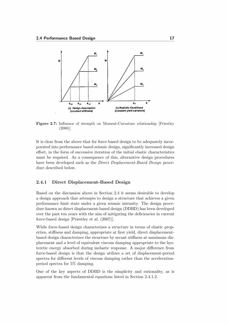
2.7 Influence of strength on Moment-Curvature relationship [Priest-ley (2000)] . . . . . . . . . . . . . . . . . . . . . . . . . . . . . 17
2.8 Fundamentals of Direct Displacement-Based Design [Priest-ley et al. (2007)] . . . . . . . . . . . . . . . . . . . . . . . . . 20
2.9 Effective stiffness ratio for large rectangular columns [Priest-ley et al. (2007)] . . . . . . . . . . . . . . . . . . . . . . . . . 22
2.10 Damping for a cantilever pier with an isolated deck [Priestleyet al. (2007)] . . . . . . . . . . . . . . . . . . . . . . . . . . . 23

x LIST OF FIGURES
2.11 Flowchart for the displacement-based design for isolated struc-tures . . . . . . . . . . . . . . . . . . . . . . . . . . . . . . . . 27
2.12 Simple flowcharts for force-based and direct displacement-based design of isolated structures . . . . . . . . . . . . . . . 28
2.13 Modified response spectrum to consider the equivalent viscousdamping of the isolation system [Priestley et al. (1996)] . . . 32
2.14 Rayleigh damping - variation of modal damping ratios withnatural frequency [Chopra (2007)] . . . . . . . . . . . . . . . 34
2.15 Strain and stress distribution and force equilibrium in a con-crete section . . . . . . . . . . . . . . . . . . . . . . . . . . . . 37
2.16 Simplified N-M interaction diagram for uniaxial bending . . . 39
3.1 Three dimensional view of the bridge . . . . . . . . . . . . . . 42
3.2 General cross section in bridge . . . . . . . . . . . . . . . . . 43
3.3 Predominant modeshapes of the original bridge in the longi-tudinal, transverse and vertical direction respectively . . . . . 46
3.4 Predominant modeshapes of the isolated bridge in the longi-tudinal, transverse and vertical direction respectively . . . . . 46
3.5 Details of LM1, placement of loads [EC1-2] . . . . . . . . . . 50
3.6 Assessment of groups of traffic loads [Table 4.4a in EC1-2] . . 50
3.7 Horizontal peak acceleration for Iceland [FS ENV 1998-1-1:1994] . . . . . . . . . . . . . . . . . . . . . . . . . . . . . . . 52
3.8 Horizontal design response spectrum. Predominant horizon-tal modes indicated with diamonds . . . . . . . . . . . . . . . 54
3.9 Vertical design response spectrum. Predominant vertical modesindicated with diamonds . . . . . . . . . . . . . . . . . . . . . 54
3.10 Displacement response spectrum used in direct displacement-based design . . . . . . . . . . . . . . . . . . . . . . . . . . . . 55
3.11 Response spectra of artificial time histories used for time his-tory analysis . . . . . . . . . . . . . . . . . . . . . . . . . . . 56
3.12 Artificial time histories created with Simqke used for timehistory analysis . . . . . . . . . . . . . . . . . . . . . . . . . . 56
4.1 Screen shot of computational model from SAP2000 . . . . . 60
4.2 Axial force and bending moment in arch due to static loads . 61

LIST OF FIGURES xi
4.3 Stresses in arch top and bottom respectively due to static loads 61
4.4 Shear force in arch due to static loads . . . . . . . . . . . . . 62
4.5 Simplified N-M interaction diagrams for piers and spandrelcolumns . . . . . . . . . . . . . . . . . . . . . . . . . . . . . . 62
4.6 Shear force in piers and spandrel columns due to static loads.Shear strength shown with dashed line . . . . . . . . . . . . . 63
4.7 Bending moment in bridge deck due to static loads . . . . . . 63
4.8 Shear force in bridge deck due to static loads . . . . . . . . . 64
4.9 Axial force and bending moment around transverse axis inarch of original bridge due to seismic loads . . . . . . . . . . . 65
4.10 Bending moment around vertical axis in arch of original bridgedue to seismic loads . . . . . . . . . . . . . . . . . . . . . . . 65
4.11 Stresses in arch top and bottom of original bridge due toseismic loads . . . . . . . . . . . . . . . . . . . . . . . . . . . 66
4.12 Vertical shear force in arch of original bridge due to seismicloads . . . . . . . . . . . . . . . . . . . . . . . . . . . . . . . . 67
4.13 Transverse shear force in arch of original bridge due to seismicloads . . . . . . . . . . . . . . . . . . . . . . . . . . . . . . . . 67
4.14 Simplified N-M interaction diagrams for piers and spandrelcolumns of original bridge. Points indicate static and seismicloaded state of columns . . . . . . . . . . . . . . . . . . . . . 68
4.15 Shear force in piers and spandrel columns of original bridgedue to seismic loads. Shear strength shown with dashed line . 68
4.16 Moment in bridge deck of original bridge due to seismic loads 69
4.17 Shear in bridge deck of original bridge due to seismic loads . 69
4.18 Axial force and bending moment around the transverse axisin the arch of base isolated bridge due to seismic loads . . . . 72
4.19 Bending moment in arch of base isolated bridge around ver-tical axis due to most severe seismic load combination . . . . 73
4.20 Stresses in arch top and bottom of base isolated bridge dueto most severe seismic load combination . . . . . . . . . . . . 74
4.21 Vertical shear force in arch of base isolated bridge due toseismic loads . . . . . . . . . . . . . . . . . . . . . . . . . . . 74

xii LIST OF FIGURES
4.22 Transverse shear force in arch of base isolated bridge due toseismic loads . . . . . . . . . . . . . . . . . . . . . . . . . . . 75
4.23 Simplified N-M interaction diagrams for piers and spandrelcolumns of base isolated bridge. Points indicate static andseismic loaded state of columns . . . . . . . . . . . . . . . . . 75
4.24 Shear force in piers and spandrel columns of base isolatedbridge due to seismic loads. Shear strength shown with dashedline . . . . . . . . . . . . . . . . . . . . . . . . . . . . . . . . . 76
4.25 Moment in bridge deck of base isolated bridge due to seismicloads . . . . . . . . . . . . . . . . . . . . . . . . . . . . . . . . 76
4.26 Shear in bridge deck of base isolated bridge due to seismic loads 76
5.1 Displacement spectra for artificial time histories and Eurocode8. Displacements in m . . . . . . . . . . . . . . . . . . . . . . 80
5.2 Hysteresis loops for LRBs . . . . . . . . . . . . . . . . . . . . 83
5.3 Displacements of deck, pier and isolator for pier no. 2 as afunction of time . . . . . . . . . . . . . . . . . . . . . . . . . . 83

List of Tables
3.1 Physical properties of lead rubber bearings . . . . . . . . . . 44
3.2 Mechanical properties of lead rubber bearings . . . . . . . . . 45
3.3 Modal analysis results of original bridge . . . . . . . . . . . . 46
3.4 Modal analysis results of isolated bridge . . . . . . . . . . . . 47
3.5 Required number of modes to reach an effective mass ratio of90% . . . . . . . . . . . . . . . . . . . . . . . . . . . . . . . . 47
3.6 Self weight of main structural elements . . . . . . . . . . . . . 48
3.7 LM1: Characteristic values . . . . . . . . . . . . . . . . . . . 49
3.8 Input to design response spectrum . . . . . . . . . . . . . . . 52
3.9 Parameters for Type 1 design response spectrum . . . . . . . 53
3.10 Recommended values of ψ factors for road bridges (EC0 A.2) 57
3.11 Combination of actions . . . . . . . . . . . . . . . . . . . . . . 57
3.12 Combinations of components of seismic action . . . . . . . . . 58
4.1 Comparison of uncracked, cracked and required stiffness forpiers . . . . . . . . . . . . . . . . . . . . . . . . . . . . . . . . 70
4.2 Comparison of displacements and deformations with RSA andDDBD (all values in mm) . . . . . . . . . . . . . . . . . . . . 71
4.3 Comparison of shear force and moment in columns with RSAand DDBD . . . . . . . . . . . . . . . . . . . . . . . . . . . . 71

xiv LIST OF TABLES
5.1 Maximum displacements [mm] from linear time history anal-ysis (LTHA) and displacement spectra (DS) . . . . . . . . . . 81
5.2 Maximum displacements and base shear from nonlinear timehistory analysis . . . . . . . . . . . . . . . . . . . . . . . . . . 82
5.3 Comparison of section forces in piers with RSA and NLTHAwith time history no. 6 . . . . . . . . . . . . . . . . . . . . . 84

Nomenclature
Abbreviations:DDBD Direct Displacement-Based DesignFBD Force Based DesignLTHA Linear Time History AnalysisMDOF Multi Degree Of FreedomNLTHA Noninear Time History AnalysisRSA Response Spectrum AnalysisSDOF Single Degree Of FreedomSIZS South Iceland Seismic Zone
Symbols not defined at each usage:
∆d Design displacement m
∆u Maximum displacement of lead rubber bearing m
∆y Yield displacement m
µd Design ductility ratio
φy Yield curvature 1m
σyL Effective yield shear stress of lead Pa
AL Cross sectional area of lead plug m2
AR Plane area of rubber m2
GR Shear modulus of rubber Pa
Keff Effective stiffness of lead rubber bearing Nm
Ke Effective stiffness of equivalent SDOF system Nm
KLR Initial stiffness of lead rubber bearing Nm

xvi LIST OF TABLES
KR Post yield stiffness of lead rubber bearing Nm
KZ Vertical stiffness of rubber bearing Nm
me Effective mass of equivalent SDOF system kg
Qy Characteristic yield strength of lead plug N
Te Effective period of equivalent SDOF system s
tR Total thickness of rubber m
Vbase Base shear N

Chapter 1
Introduction
1.1 Background
A preliminary design of a concrete arch bridge was performed by the authorof this thesis in the course “11373 - Bridge Design”, taught at the TechnicalUniversity of Denmark in the fall of 2008. The bridge was supposed to beconstructed in Finland and hence no consideration was made on seismicdesign. In this thesis the consequences of erecting the bridge in the SouthIcelandic Seismic Zone (SISZ) will be examined.
Iceland is located on the Mid Atlantic Ridge and is being split by the diver-gent plate boundary between the North American Plate and the EurasianPlate which causes regular earthquakes and eruptions. Two main seismiczones exist in Iceland, the Tjornes Fracture Zone (TFZ) and the South Ice-land Seismic Zone. The most destructive earthquakes have been recordedin these two zones.
Bridges are lifeline structures, important links in the infrastructure and theirfailure during an earthquake will seriously hamper relief and rehabilitationwork. It is therefore important that bridges exposed to severe earthquakescan survive without serious damage and be opened for traffic quickly. Fail-ures to bridges due to complete failure of their piers or other structuralelements have been observed in every major seismic event, e.g. in Hyogo-ken Nanbu in 1995 [Jangid (2004)], San Fernandi in 1971 [Dusseau and Wen(1989)], Northridge in 1994 [Priestley et al. (1996)] to name a few. Evenbridges designed specifically for seismic resistance have collapsed or havebeen severely damaged when subjected to ground shaking of an intensity of-

2 Introduction
Figure 1.1: Recorded earthquakes in Iceland in 2003
ten less than that corresponding to current code intensities [Priestley et al.(1996)].
To increase the safety of bridges during a seismic event a relatively newmethod in earthquake-resistant design has been developed called seismic iso-lation. Scientists and engineers in New Zealand, the United States, Japanand Italy have been active in developing the concept and using it in bothbuildings and bridges [Skinner (1993), Naeim and Kelly (1999)]. Many iso-lations systems have been proposed through the years (see e.g. [Naeim andKelly (1999)]) and they all aim at reducing the earthquake damage potentialby uncoupling the structure from the damaging action of the earthquake.The most commonly used isolators today are lead rubber bearings as theyprovide an economic, reliable and simple solution for protecting medium andshort span bridges [Jara and Casas (2006), Bessason and Haflidason (2004)].Lead rubber bearings have been used in all 15 seismically isolated bridgesin Iceland [Jonsson et al. (2010)].
In June 2000 two major earthquakes struck the South Iceland Seismic Zonewith magnitudes MW = 6.6 and MW = 6.5. During these earthquakes theresponse of a recently seismically upgraded bridge with seismic isolation wasrecorded. The bridge was instrumented with accelerometers monitoring theground motion as well as the structural response. The bridge survived bothearthquakes without any serious damage but numerical analysis strongly

1.1 Background 3
Figure 1.2: A collapsed part of the Hanshin Expressway from the Hyogo-kenNanbu earthquake in 1995
indicated that without the base isolation the bridge would have been severelydamaged or even collapsed [Bessason and Haflidason (2004)]. In May 2008another earthquake hit South Iceland (MW=6.3). The base isolated Oseyrarbridge was subjected to strong near-fault ground motion and experiencedsome damage but was opened for traffic only few hours after the earthquake[Jonsson et al. (2010)].
Damage of bridges during the Hyogo-ken Nanbu (Kobe) earthquake in 1995attracted considerable attention among researches realizing that strengthalone would not be sufficient for the safety of bridges [Jangid (2004)]. Thishas lead to a demand for a different approach to seismic design and to-day it is widely recognized that seismic design codes need to incorporate aperformance-based design criterion. A simple but reliable conceptual frame-work called direct-displacement based design has been proposed for achievingthe performance based design objective. It is generally agreed that deforma-tions are more critical parameters for defining performance, and as a resultit is argued that seismic design methods should largely be based on them. Incontrast to force-based design, the end result of the displacement-based de-sign procedure is the required stiffness, which is determined from the elasticspectrum by means of maximum total displacement and equivalent dampingof the system.

4 Introduction
1.2 Objectives
This thesis has two main objectives. The first is to extend the preliminarydesign of a concrete arch bridge, made in the course“11373 - Bridge Design”,to include a seismic design and to study how the application of seismicloading affects the design concept. Instead of the original position of thebridge in Finland, the bridge is analyzed for a code-specified seismic load insouth of Iceland.
The second main objective of this thesis is to employ the direct displacement-based design approach to design a base isolation system for the bridge andcompare it to the traditional force-based design. The accuracy of simplehand calculations, proposed by the direct displacement-based design ap-proach, is assessed with response spectrum and nonlinear time history anal-ysis.
The main chapters are as follows:
Second chapter: The basic theory used is presented. Basics of structuraldynamics, definition of seismic load with response spectra and time histo-ries, seismic isolation, performance based design, basics of Eurocode 8 andultimate strength of elements.
Third chapter: The analyzed bridge is described in detail as well as theisolation devices. The applied load is defined.
Fourth chapter: Static and linear dynamic analysis of the original and theisolated bridge. The calculation process is described and results presented.
Fifth chapter: Time history analysis of the isolated bridge is described andmain findings presented.
Sixth chapter: Summary and conclusions.
Chapter 2
Theory
2.1 Equations of Motion
2.1.1 Single Degree of Freedom
The response of a linear single degree of freedom (SDOF) system to groundmotions ug is the solution to the differential equation [Chopra (2007)]
mu+ cu+ ku = −mug (2.1)
where m is the mass of the system, c is the damping constant and k isthe stiffness. Relative displacement of the system as a function of time isdenoted u(t). First derivative of the displacement is the velocity u(t) andthe second derivative is the acceleration of the system u(t).
By dividing the equation above with the mass m the normalized equationof motion is obtained.
u+ 2ζω0u+ ω20u = −ug (2.2)
where ω0 is the natural angular frequency and ζ is the damping ratio of thesystem.
ω0 =√
km ζ =
c
2√km
(2.3)
6 Theory
The relation between period T and natural angular frequency ω0 is given by
T =2πω0
= 2π√
mk (2.4)
2.1.2 Multiple Degrees of Freedom
The dynamic behavior of most structures involves simultaneous motion ofseveral masses in shapes that are not known before the analysis. Thus, thetheory of dynamics of a single degree of freedom must be extended to dealwith several masses and systems with distributed mass like beam and framestructures, as well as complete buildings and structures such as bridges.
The first extension of the theory is from one degree of freedom involving asingle mass to multiple degrees of freedom, describing the coupled motionof several concentrated masses. This theory is called modal analysis andincludes terms such as mode shapes, modal mass and modal stiffness.
The objective of modal analysis is to determine combined motion of massesthat will retain the same combination during free vibrations and to deter-mine the corresponding frequency, loading conditions etc.
The dynamic response of a linear system with n degrees of freedom u(t)T =[u1(t), u2(t), ..., un(t)] to ground motions is described by the set of secondorder differential equations
mu + cu + ku = −mIug (2.5)
The physical parameters are: the mass matrix m, the viscous damping ma-trix c and the stiffness matrix k. Effective earthquake forces are given by thevector −mIug where I is the influence vector representing the displacementsof the masses resulting from static application of a unit ground displacement.
Mode shapes and periods are found by solving the generalized eigenvalueproblem
(k− ω2m
)φ = 0 (2.6)
The complete solution to the generalized eigenvalue problem consists of nsets of eigenvalues and eigenvectors, arranged as corresponding pairs of nat-ural frequency ωj and mode shape vector φj .
ωj , φj j = 1, 2, ..., n (2.7)
2.2 Definition of Seismic Load 7
Traditionally the mode shapes are ordered with respect to increasing magni-tude of the associated natural frequency. The generalized eigenvalue prob-lem does not determine the magnitude of the modeshape vectors. They cantherefore be normalized by multiplication with a suitable scaling factor.
Modal mass and modal stiffness corresponding to mode j are defined as
mj = φTj mφj kj = φTj kφj (2.8)
The eigenfrequency ωj can be expressed by the ratio of modal stiffness tomodal mass by premultiplication of the generalized eigenvalue equation withφTj . This relation is called Rayleigh’s quotient and generalizes the definitionof the angular frequency for a SDOF system [Chopra (2007)].
ω2j =
φTj kφjφTj mφj
=kjmj
(2.9)
2.2 Definition of Seismic Load
2.2.1 Time Histories
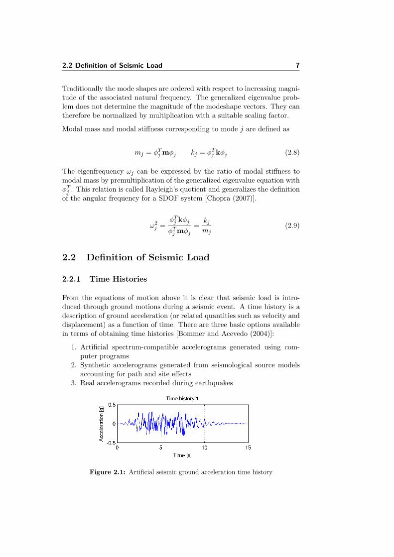
From the equations of motion above it is clear that seismic load is intro-duced through ground motions during a seismic event. A time history is adescription of ground acceleration (or related quantities such as velocity anddisplacement) as a function of time. There are three basic options availablein terms of obtaining time histories [Bommer and Acevedo (2004)]:
1. Artificial spectrum-compatible accelerograms generated using com-puter programs
2. Synthetic accelerograms generated from seismological source modelsaccounting for path and site effects
3. Real accelerograms recorded during earthquakes
Figure 2.1: Artificial seismic ground acceleration time history
8 Theory
The first option listed above is the one used in this thesis. Artificial accelero-grams are created using the Matlab program SimSeisme [Lestuzzi (2002)]based on the well know program Simqke, created by Gasparini and Vanmar-cke. This option was chosen to obtain time histories with response spectrasimilar to the smooth EC8 design spectrum for comparison of the results ob-tained using response spectrum analysis with isolating devices representedwith linear equivalent properties and the time history analysis with nonlin-ear modeling of the isolation devices. The approach employed in Simqke isto generate a power spectral density function from the smoothed responsespectrum of EC8 (or some other target spectrum) and then derive sinusoidalsignals having random phase angles and amplitudes. The sinusoidal motionsare then summed and an iterative procedure can be invoked to improve thematch with the target response spectrum by calculating the ratio betweenthe target and actual response ordinates at selected frequencies. The powerspectral density function is then adjusted by the square of this ratio, and anew motion is generated. By doing so it is possible to obtain accelerationtime histories that are almost completely compatible with the elastic designspectrum.
2.2.2 Response Spectrum
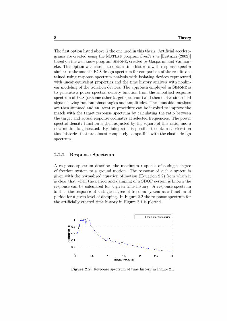
A response spectrum describes the maximum response of a single degreeof freedom system to a ground motion. The response of such a system isgiven with the normalized equation of motion (Equation 2.2) from which itis clear that when the period and damping of a SDOF system is known theresponse can be calculated for a given time history. A response spectrumis thus the response of a single degree of freedom system as a function ofperiod for a given level of damping. In Figure 2.2 the response spectrum forthe artificially created time history in Figure 2.1 is plotted.
Figure 2.2: Response spectrum of time history in Figure 2.1
2.3 Seismic Isolation 9
2.3 Seismic Isolation
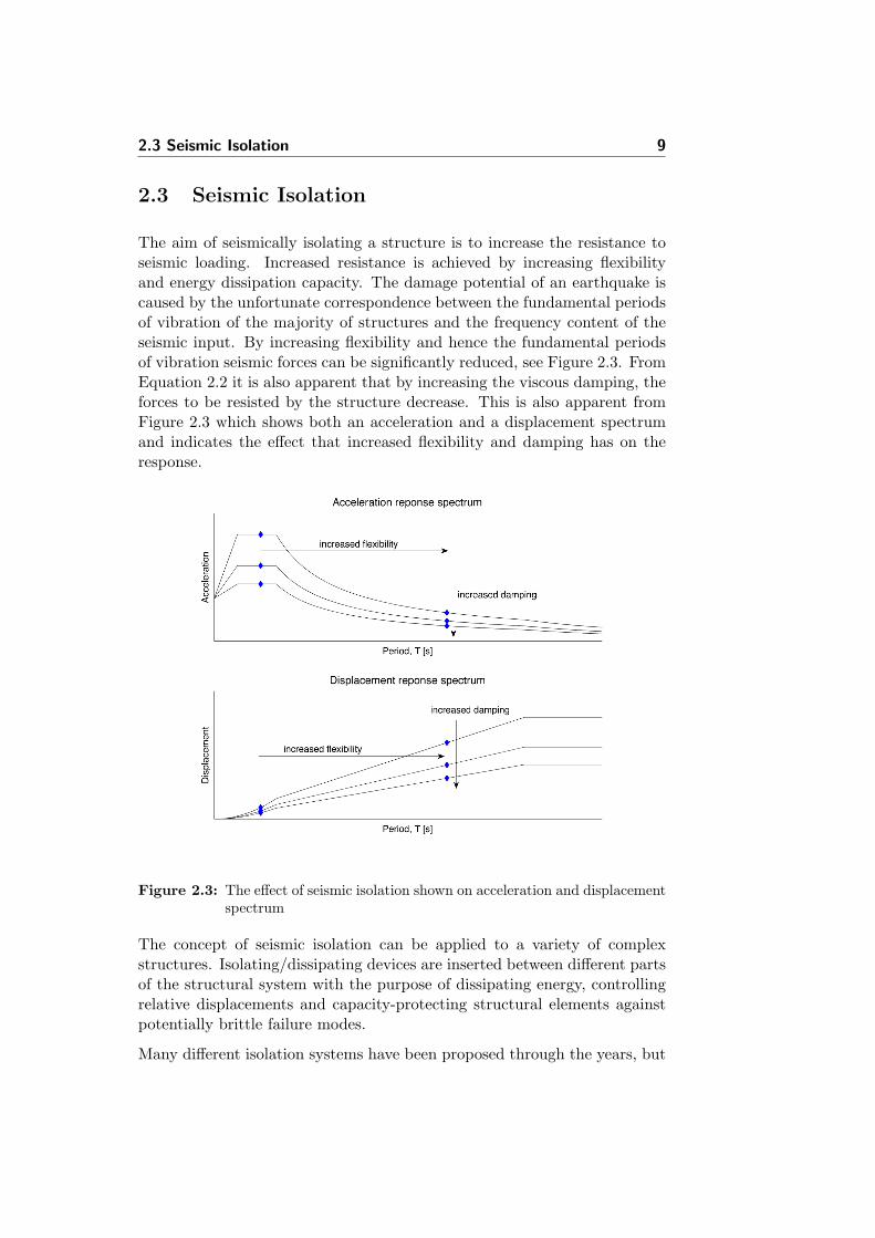
The aim of seismically isolating a structure is to increase the resistance toseismic loading. Increased resistance is achieved by increasing flexibilityand energy dissipation capacity. The damage potential of an earthquake iscaused by the unfortunate correspondence between the fundamental periodsof vibration of the majority of structures and the frequency content of theseismic input. By increasing flexibility and hence the fundamental periodsof vibration seismic forces can be significantly reduced, see Figure 2.3. FromEquation 2.2 it is also apparent that by increasing the viscous damping, theforces to be resisted by the structure decrease. This is also apparent fromFigure 2.3 which shows both an acceleration and a displacement spectrumand indicates the effect that increased flexibility and damping has on theresponse.
Figure 2.3: The effect of seismic isolation shown on acceleration and displacementspectrum
The concept of seismic isolation can be applied to a variety of complexstructures. Isolating/dissipating devices are inserted between different partsof the structural system with the purpose of dissipating energy, controllingrelative displacements and capacity-protecting structural elements againstpotentially brittle failure modes.
Many different isolation systems have been proposed through the years, but
10 Theory
systems based on elastomeric bearings are most common. In a typical iso-lated bridge, special isolation devices are used in place of the conventionalbridge bearings or monolithic connections between piers and bridge deck.The suitability of a particular arrangement and type of isolation system willdepend on many factors, including the span length, number of continuousspans, seismicity of the region, maintenance and replacement facilities. Com-mon isolation devices include elastomeric bearings, lead rubber bearings,high-damping rubber bearings and friction pendulum systems. Dampingcan either be included in the devices or provided with secondary mechanicaldevices.
2.3.1 Lead Rubber Bearings
Lead rubber bearings are low-damping laminated rubber bearings with alead plug inserted in the core of the device. The purpose of the lead plugis to increase the stiffness at relatively low horizontal force levels as well asto increase energy dissipation capacity of the bearing. The horizontal force-displacement curve is a combination of the linear response of the rubberbearing and the essentially elastic-perfectly plastic response of a confinedlead plug. A lead rubber bearing thus combines the displacement capacityof the rubber with hysteretic energy dissipation of the lead plug providingthe damping required for a seismic isolation system to be efficient. Undernormal conditions they behave like regular bearings but in the event of astrong earthquake, they add flexibility to the structure by elongating itsperiod and dissipate energy.
Lead rubber bearings were invented in New Zealand during the mid 1970sby W.H Robinson [Skinner (1993)]. Since then they have grown to becomethe most common isolation devices for bridges and up until now all the seis-mically isolated bridges in Iceland are using lead rubber bearings [Bessasonand Haflidason (2004)].
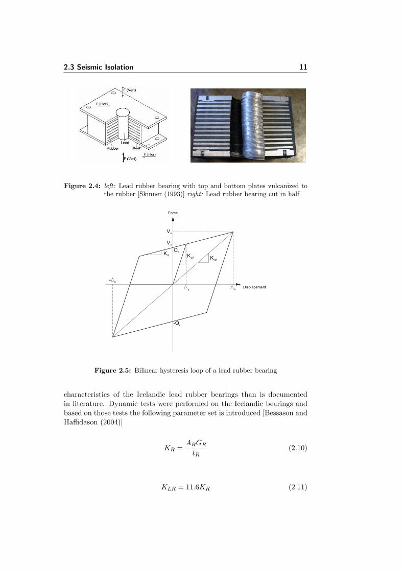
A reasonable description of the hysteresis loop of a lead rubber bearing is abilinear solid with an initial elastic stiffness of KLR followed by a post yieldstiffness of KR, see Figure 2.5. Also shown in Figure 2.5 is the characteristicyield strength of the lead plug at zero strain Qy, effective stiffness Keff ,yield and maximum displacement, ∆y and ∆u, as well as the correspondingyield and maximum strength, Vy and Vu.
The common way to insert the lead plug into the elastomeric bearing isto manufacture a bearing with a hole and then press an oversized lead pluginto it. However, in Iceland a non-traditional method has been used where ahole is drilled into a conventional elastomeric bearing, and subsequently thelead plug is cast directly into the hole. This results in somewhat different
2.3 Seismic Isolation 11
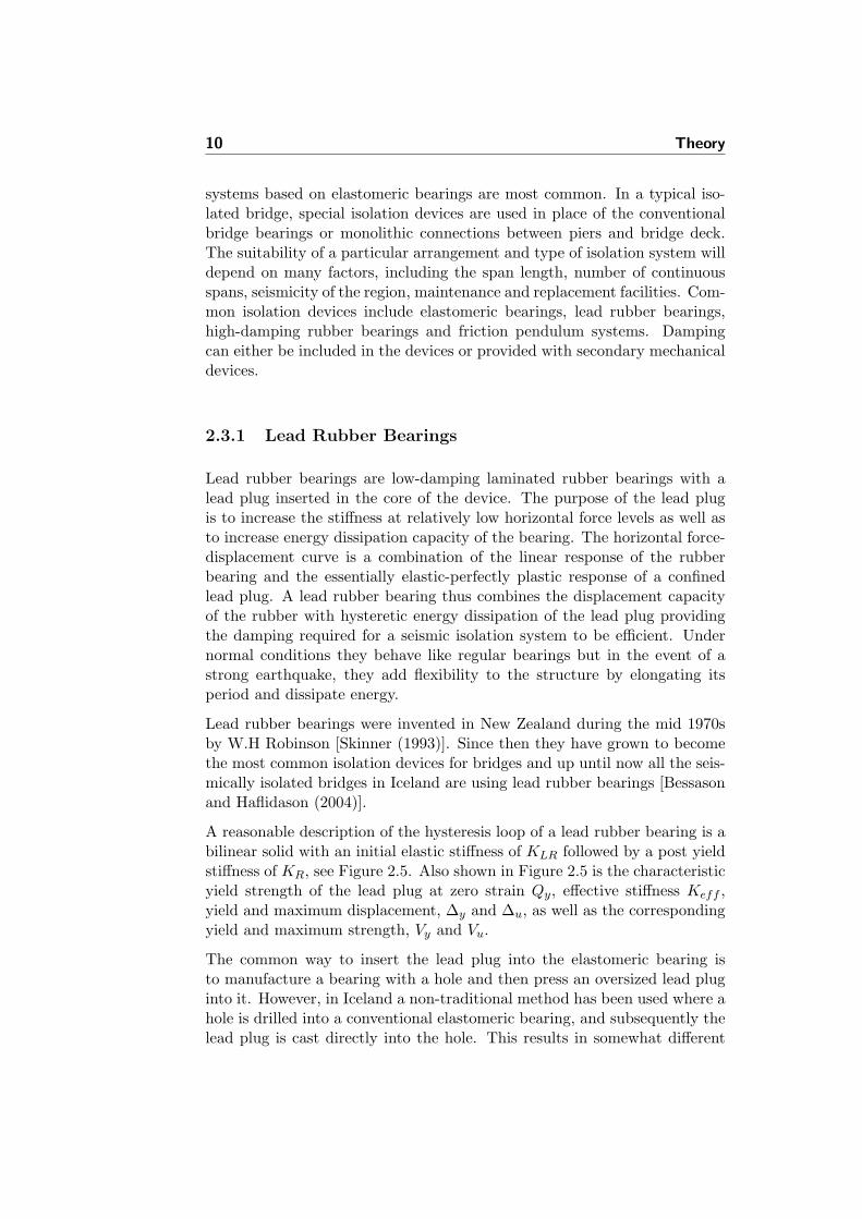
Figure 2.4: left: Lead rubber bearing with top and bottom plates vulcanized tothe rubber [Skinner (1993)] right: Lead rubber bearing cut in half
Figure 2.5: Bilinear hysteresis loop of a lead rubber bearing
characteristics of the Icelandic lead rubber bearings than is documentedin literature. Dynamic tests were performed on the Icelandic bearings andbased on those tests the following parameter set is introduced [Bessason andHaflidason (2004)]
KR =ARGRtR
(2.10)
KLR = 11.6KR (2.11)
12 Theory
Qy = σyLAL (2.12)
where AR is the plane area, GR is the shear modulus and tR is the totalthickness of the rubber in the bearing. AL is the cross sectional area of leadplug and σyL is the estimated effective yield shear stress of the lead plug. Theparameter 11.6 in Equation 2.11 is higher than normally found in literaturewhere it has been reported to be approximately 10 (see e.g. [Skinner (1993),Jara and Casas (2006), Naeim and Kelly (1999)]). The effective yield shearstress of the lead plug was determined as σyL = 8.0 MPa which is about 20%lower than documented elsewhere. The variation in these parameters canbe explained by the different method of inserting the lead plug as discussedabove. Yield displacement can be derived from the bilinear representation
∆y =Qy
KLR −KR(2.13)
The amount of lead is often expressed as the ratio of rubber to lead, asshown in Equation 2.14. Typical values of n range from 10-20 [Jara andCasas (2006), Priestley et al. (2007)].
n =ARAL
(2.14)
Vertical load capacity of an elastomeric bearing is usually expressed by thefollowing equation [Priestley et al. (2007), Skinner (1993)]
W ≤ A′GRSγ (2.15)
where W is the allowable weight, γ is the allowable shear strain, A′ is theminimum permitted overlap of top and bottom area of the bearing at max-imum displacement (taken as AR
2 ) and S is a shape factor equal to loadedarea divided by force free area.
Allowable maximum rubber shear strain without lead plug is given as
γ = 0.4εt (2.16)
where εt is the short-duration failure strain in simple tension. Experimentssuggest this factor as a minimum for design-earthquakes and up to 0.7 forextreme earthquakes. The short-duration failure strain in simple tension can

2.3 Seismic Isolation 13
be taken as εt = 350% [Skinner (1993)], although these characteristics shouldof course be determined based on tests on a sample prior to installation. Thismeans that the allowable maximum rubber shear strain is in the interval140% - 245%. The lowest value is used here as stated in Equation 2.16.
Vertical stiffness of rubber bearings is given with [Priestley et al. (1996),Priestley et al. (2007)]
KZ =6GRS2ARkb
(6GRS2 + kb)tR(2.17)
where kb is the rubber bulk modulus, taken as 2000 MPa and the othersymbols as already defined. The vertical stiffness calculated with Equation2.17 considers the sum of the deflection due to the rubber shear strain andthe rubber volume change.
2.3.1.1 Equivalent Linear Model
The response spectrum provides some of the most important characteristicsof earthquake motion and gives the maximum elastic deformation for struc-tures over the entire range of periods. However, it is not able to predictdamage level, as damage involves inelastic deformations. Inelastic responsecan be captured through nonlinear time history analysis, but in many casesthe linear response spectrum is the preferred weapon of choice for practicingengineers. Hence approximate methods have been developed to describe theisolators with equivalent linear models using effective lateral stiffness andequivalent damping ratio. Equivalent linear models have been incorporatedin Eurocode 8 for designing bridges with passive energy dissipation systemsas well as other codes.
The behavior of an inelastic hysteretic structure subjected to ground accel-eration ug is assumed to be described by a single degree of freedom systemand the maximum inelastic response is given as [Jara and Casas (2006)]
u+ 2ζiωiu+fs(u, u)m
= −ug (2.18)
where ζi is the damping ratio, ωi is the initial circular frequency and fs(u, u)is the restoring force. In the equivalent linearization method, the maximuminelastic displacement demand ueq is approximated by
ueq + 2ζeqωef ueq + ω2efueq = −ug (2.19)
14 Theory
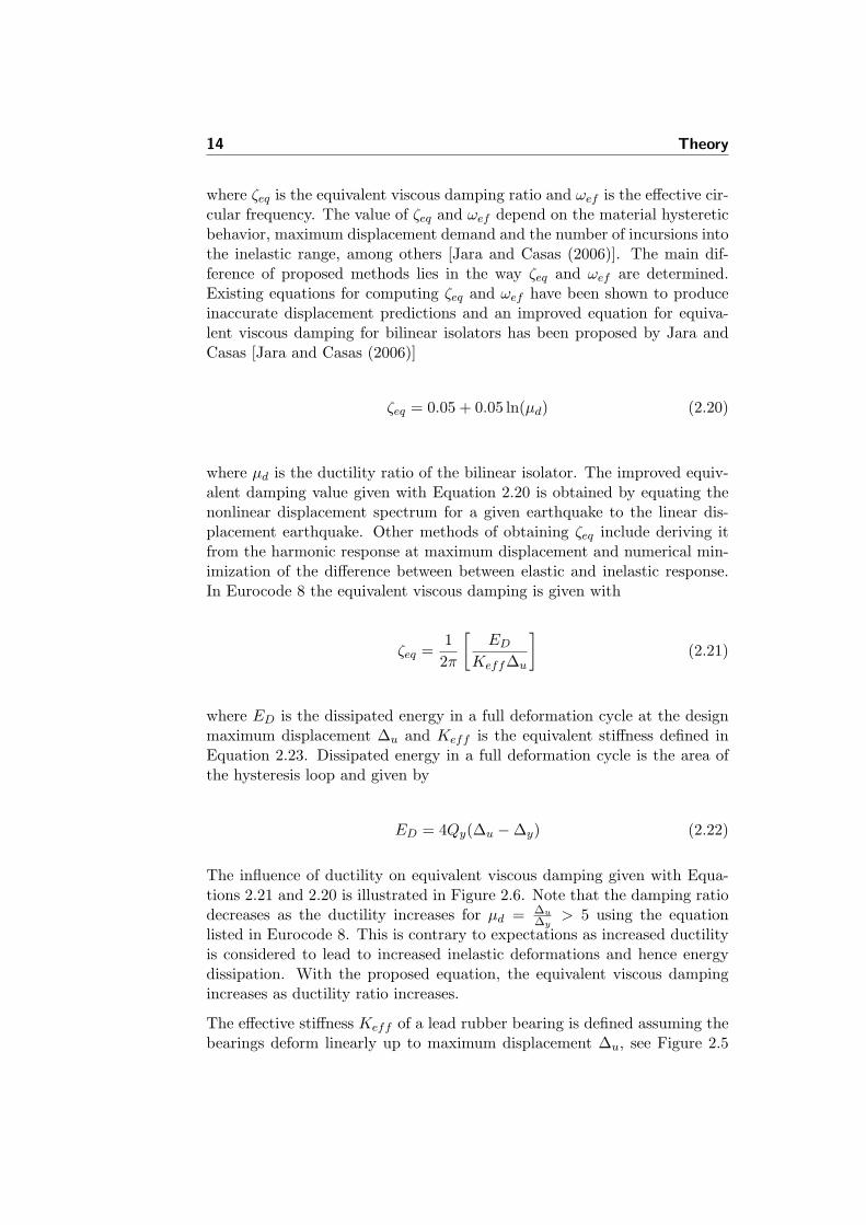
where ζeq is the equivalent viscous damping ratio and ωef is the effective cir-cular frequency. The value of ζeq and ωef depend on the material hystereticbehavior, maximum displacement demand and the number of incursions intothe inelastic range, among others [Jara and Casas (2006)]. The main dif-ference of proposed methods lies in the way ζeq and ωef are determined.Existing equations for computing ζeq and ωef have been shown to produceinaccurate displacement predictions and an improved equation for equiva-lent viscous damping for bilinear isolators has been proposed by Jara andCasas [Jara and Casas (2006)]
ζeq = 0.05 + 0.05 ln(µd) (2.20)
where µd is the ductility ratio of the bilinear isolator. The improved equiv-alent damping value given with Equation 2.20 is obtained by equating thenonlinear displacement spectrum for a given earthquake to the linear dis-placement earthquake. Other methods of obtaining ζeq include deriving itfrom the harmonic response at maximum displacement and numerical min-imization of the difference between between elastic and inelastic response.In Eurocode 8 the equivalent viscous damping is given with
ζeq =1
2π
[ED
Keff∆u
](2.21)
where ED is the dissipated energy in a full deformation cycle at the designmaximum displacement ∆u and Keff is the equivalent stiffness defined inEquation 2.23. Dissipated energy in a full deformation cycle is the area ofthe hysteresis loop and given by
ED = 4Qy(∆u −∆y) (2.22)
The influence of ductility on equivalent viscous damping given with Equa-tions 2.21 and 2.20 is illustrated in Figure 2.6. Note that the damping ratiodecreases as the ductility increases for µd = ∆u
∆y> 5 using the equation
listed in Eurocode 8. This is contrary to expectations as increased ductilityis considered to lead to increased inelastic deformations and hence energydissipation. With the proposed equation, the equivalent viscous dampingincreases as ductility ratio increases.
The effective stiffness Keff of a lead rubber bearing is defined assuming thebearings deform linearly up to maximum displacement ∆u, see Figure 2.5

2.4 Performance Based Design 15
Figure 2.6: Equivalent damping from Eurocode 8 and proposed improved equa-tion by Jara and Casas
[Naeim and Kelly (1999), Jara and Casas (2006)]
Keff =Qy∆u
+KR (2.23)
2.4 Performance Based Design
One of the major developments in seismic design over the past twenty yearshas been increased emphasis on limit states design, now generally termedPerformance Based Engineering [Priestley (2000)]. Several techniques havebeen developed and now three of them have developed to a stage where seis-mic assessment of existing structures, or design of new structures can be car-ried out to ensure that particular deformation-based criteria are met. Theseare the capacity spectrum approach, N2 method and direct displacement-based design. They all follow from the realization that increasing strengthmay not enhance safety nor necessarily reduce damage and focus on movingthe emphasis in design from “strength” to “performance”.
The start of performance based seismic engineering can be tracked back tothe 1970s and the development of capacity design principles in New Zealand.It was then realized that the distribution of strength through a buildingwas more important than the absolute value of the design base shear. Theweak-beam/soft-column philosophy was realized to perform better duringa seismic event as well as the importance of the shear strength exceed-ing the corresponding flexural strength. This philosophy of controlling theoverall performance of the building as a function of the design process can
16 Theory
be identified as the true start to performance based seismic design. It istoday widely recognized that seismic design codes need to incorporate aperformance-based design criterion [Priestley (2000)].
The traditional force-based design approach includes some conceptual andphilosophical problems, some of which are listed below [Priestley (2000)]
• It is generally accepted that damage is strain related for structural com-ponents, or drift related for non-structural components. There is no clearrelationship between strength and damage.
• Use of force-reduction or ductility factors for design results in non-uniformrisk, since ductility is a poor indicator of damage potential. Thus two differentbuildings designed to the same code and with the same force-reduction orductility factors may experience different levels of damage under a givenearthquake.
• For many structures, code drift limits will be found to govern and as a con-sequence force-reduction factors will be less than code indicative limits. Thisimplies the need for iterative design and increased design complexity.
• Force-based design requires the specification of initial stiffness of structuralmembers. Forces are then distributed between structural members on thebasis of initial stiffness. This is sometimes taken to be gross stiffness, andsometimes as a reduced stiffness to represent the influence of cracking inconcrete and masonry structures. This implies that the structural stiffnessis independent of strength for a given gross member dimension and thatyield displacement, or yield curvature, is directly proportional to strength,as shown in Figure 2.7(a). Detailed analysis and experimental evidence showthat this assumption is invalid, in that stiffness is essentially directly pro-portional to strength, and the yield displacement or curvature is essentiallyindependent of strength as shown in Figure 2.7(b). It has been found possibleto express the yield curvature of different reinforced concrete structural mem-bers by dimensionless relationships, see Equation 2.25 in Section 2.4.1.1. Asa consequence of this it is not possible to perform an accurate analysis of ei-ther the structural period, nor of the elastic distribution of required strengththrough the structure, until the member strengths have been defined. Sincethese aspects are the fundamental basis for force-based design, the implica-tion is that successive iteration must be carried out before an adequate elasticcharacterization of the structure is obtained.
• The assumption that the elastic characteristics of the building are the bestindicator of inelastic performance, as implied by force-based design, is clearlyof doubtful validity. The reason for sticking with this approach is thought tobe historical - seismic design started on the basis of simple elastic analysisin the 1930s, and the appreciation that it is displacement capacity, ratherthan strength, that is more fundamental to seismic performance, has notbeen general for sufficient time for the fundamental basis of seismic design,namely initial stiffness characterization, to have been clearly examined anddiscarded.
2.4 Performance Based Design 17
Figure 2.7: Influence of strength on Moment-Curvature relationship [Priestley(2000)]
It is clear from the above that for force-based design to be adequately incor-porated into performance based seismic design, significantly increased designeffort, in the form of successive iteration of the initial elastic characteristicsmust be required. As a consequence of this, alternative design procedureshave been developed such as the Direct Displacement-Based Design proce-dure described below.
2.4.1 Direct Displacement-Based Design
Based on the discussion above in Section 2.4 it seems desirable to developa design approach that attempts to design a structure that achieves a givenperformance limit state under a given seismic intensity. The design proce-dure known as direct displacement-based design (DDBD) has been developedover the past ten years with the aim of mitigating the deficiencies in currentforce-based design [Priestley et al. (2007)].
While force-based design characterizes a structure in terms of elastic prop-erties, stiffness and damping, appropriate at first yield, direct displacement-based design characterizes the structure by secant stiffness at maximum dis-placement and a level of equivalent viscous damping appropriate to the hys-teretic energy absorbed during inelastic response. A major difference fromforce-based design is that the design utilizes a set of displacement-periodspectra for different levels of viscous damping rather than the acceleration-period spectra for 5% damping.
One of the key aspects of DDBD is the simplicity and rationality, as isapparent from the fundamental equations listed in Section 2.4.1.2.

18 Theory
2.4.1.1 Design Displacement
Determining the design displacement is for obvious reasons an importantstep in the direct displacement-based design procedure. It is selected con-sidering the actual displacement spectra which is a function of local seis-micity as well as functional requirements, see Section 3.2.4.1. Design dis-placement depends on the limit state considered and whether structural ornon-structural considerations are more critical. For any given limit statestructural performance will be governed by limiting material strains, sincedamage is strain-related for structural elements. Damage to non-structuralelements are generally drift related. Calculating design displacement fromstrain limits is generally straightforward.
The determination of design displacement depends on the structure beinganalyzed. For an isolated bridge, as is the case in this thesis, the designdisplacement consists of two terms; pier displacement and bearing displace-ment.
∆d = ∆B + ∆P (2.24)
In Equation 2.24, ∆B is the design deformation of the bearing and ∆P isthe displacement of the pier top. The design displacement of lead rubberbearings is limited by shear strains in the rubber as discussed in Section 2.3.1whereas the pier displacement is bounded by a choice made by the designer.An important reason for isolating a bridge is to protect the substructurefrom brittle failure modes and therefore it is desirable to limit the pierdisplacements to remain within the elastic range. Hence, pier displacementsshould be limited to a fraction of their yield displacement. This is discussedfurther in Section 2.4.1.4.
Experimental results discussed further in Section 2.4.1.3 indicate that yieldcurvature is essentially independent of reinforcement content and axial loadlevel, and is a function of yield strain and section depth alone. Yield curva-ture for a rectangular concrete column can be approximated with
φy =2.10εyhc
(2.25)
where εy is the yield strain of the flexural reinforcement and hc is the sec-tion depth. The equation above is given for solid rectangular sections butcan be used as a reasonable estimate for hollow columns [Priestley et al.(2007)]. Hence, for a SDOF vertical cantilever the yield displacement can
2.4 Performance Based Design 19
be satisfactorily approximated for design purposes by the following equation[Priestley et al. (2007)]
∆y =φy(H + Lsp)2
3(2.26)
where H is the cantilever height and Lsp is the strain penetration lengthgiven with Equation 2.27.
Lsp = 0.022fyddlb (2.27)
where fyd and dlb are the yield strength and diameter of longitudinal rein-forcement respectively.
2.4.1.2 Fundamentals
As mentioned above, direct displacement-based design characterizes thestructure to be designed by a SDOF representation of performance at peakdisplacement response, rather than by its initial elastic characteristics. Thisis based on the substitute structure approach developed by Shibata and Sozen[Priestley (2000)]. The design method is described with reference to Figure2.8, which considers a SDOF representation of a multistory building (thebasic fundamentals apply to all structural types). The bilinear envelope ofthe lateral force-displacement response of the SDOF representation is shownin Figure 2.8(b). An initial stiffness Ki is followed by a post yield stiffnessrKi. DDBD characterizes the structure by secant stiffness Ke at maximumdisplacement ∆d and a level of equivalent viscous damping ζeq (ξ in figure),representative of the combined elastic damping and the hysteretic energyabsorbed during inelastic response.
Having determined the design displacement at maximum response and es-timated corresponding damping from the expected ductility demand, theeffective period Te can be easily read from a displacement-period spectra asshown in Figure 2.8(d). The effective stiffness Ke of the equivalent SDOFsystem at maximum displacement can be found by inverting the equationfor the period of a SDOF oscillator given by Equation 2.4 to provide
Ke =4π2me
T 2e
(2.28)
where me is the effective mass of the structure participating in the funda-mental mode of vibration. Design lateral force, which is also the design base

20 Theory
Figure 2.8: Fundamentals of Direct Displacement-Based Design [Priestley et al.(2007)]
shear force is thus simply
Vbase = Ke∆d (2.29)
The design concept is thus very simple. The complexity does however stillexists and relates to determination of the substitute structure characteristics,design displacement and development of displacement spectra. Also thedistribution of design base force to the different discretized mass locationsneeds careful consideration.
2.4.1.3 Elastic Stiffness of Cracked Concrete Sections
In direct displacement-based design the required stiffness is the output ofthe design, whereas in force-based design the total base shear is distributedto the structural elements in proportion to their stiffness. A fundamentalassumption in the force-based design approach is the estimated stiffness ofthe structure which is used for the determination of the natural period of the
2.4 Performance Based Design 21
structure and the distribution of forces to different elements. This stiffnessis not known initially so in the force-based design an estimate is made.Eurocode 8 states that the cracked stiffness can be taken as one-half ofinitial elastic stiffness if no other analysis is conducted. Uncracked stiffnessfor top transverse displacement of a cantilever pier, of height H, havingmodulus of elasticity E and moment of inertia I, subjected to transverseend force is given with [Jensen (2003)]
k =3EIH3
(2.30)
The effective or cracked section moment of inertia Ie should be used toreflect the cracked state of a concrete column. The effective stiffness EIedoes not reflect only the effect of cracking but also the state of a bridgecolumn determined at first theoretical yield of the reinforcement and canbe determined from sectional moment-curvature analysis as [Priestley et al.(1996)]
EIe =Myi
φyi(2.31)
In Equation 2.31, Myi and φyi represent the ideal yield moment and cur-vature for a bilinear moment-curvature approximation. Idealized moment-curvature relationship is shown in Figure 2.7.
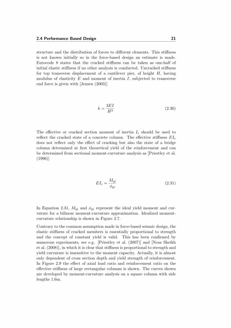
Contrary to the common assumption made in force-based seismic design, theelastic stiffness of cracked members is essentially proportional to strengthand the concept of constant yield is valid. This has been confirmed bynumerous experiments, see e.g. [Priestley et al. (2007)] and [Neaz Sheikhet al. (2008)], in which it is clear that stiffness is proportional to strength andyield curvature is insensitive to the moment capacity. Actually, it is almostonly dependent of cross section depth and yield strength of reinforcement.In Figure 2.9 the effect of axial load ratio and reinforcement ratio on theeffective stiffness of large rectangular columns is shown. The curves shownare developed by moment-curvature analysis on a square column with sidelengths 1.6m.
22 Theory
Figure 2.9: Effective stiffness ratio for large rectangular columns [Priestley et al.(2007)]
The constant yield curvature assumption makes determination of the ef-fective stiffness possible once the yield curvature and flexural strength areknown. This can be seen from Figure 2.7(b), which shows the momentcurvature relationship, and Equation 2.31.
2.4.1.4 Displacement-Based Design of Isolated Bridges
Applying direct displacement-based design to isolated bridges seems to be alogical approach since the emphasis is on the displacement rather than theforces transmitted through the device. The superstructure is presumed tobe relatively rigid in comparison with the stiffness of piers and abutmentsand it is assumed that dynamic response of the bridge can be predicted quiteaccurately with a SDOF system. A sketch of the idealized model is shownin Figure 2.10.
Generally a preliminary design of the bridge has been performed consideringnon-seismic loading conditions and therefore a full geometry is available andpossibly a preliminary dimensioning of reinforcement. Yield displacementsof each pier can then be calculated applying Equation 2.26. The isolationsystem should be designed having a yield displacement such that the equiv-alent yield point for the pier-isolator system should correspond to a forcelevel equal to a desired fraction of pier yield to ensure elastic response of thepiers.
∆d = ∆B +X∆yP (2.32)

2.4 Performance Based Design 23
In Equation 2.32, ∆B is the design displacement of the bearing, ∆yP is theyield displacement of the pier and X is the fraction of pier yield displacementchosen. Typically this value is chosen to be 80% to ensure that yield doesnot occur in the piers. The design process will imply the definition of auniform design displacement of the deck. This uniform displacement willcorrespond to different combinations of column and bearing displacementfor each pier. As a consequence different equivalent viscous damping valueswill also exist for each pier-isolator system.
Figure 2.10: Damping for a cantilever pier with an isolated deck [Priestley et al.(2007)]
At the limit-state response the lateral force may be essentially the sameas yield or it may be significantly larger depending on isolator properties.Pier deformation will increase in proportion to the force increase while thebearing will increase 10-15 times depending on accepted plastic deformationsassociated with the limit strains [Priestley et al. (2007)]. This is indicatedin Figure 2.10 where ∆yS is the equivalent yield displacement of the system,∆yB is the yield displacement of the device, ∆dP and ∆dB are the designdisplacements of the pier and bearing, respectively.
Equivalent viscous damping for the pier-isolator system is a combination ofelastic damping of the pier and hysteretic damping of the isolator. Elastic

24 Theory
damping ratio is taken as ζel = 5% which is commonly used for concrete.
ζP.i =ζB∆B.i + ζel∆dP.i
∆d(2.33)
In Equation 2.33, ζB and ∆B.i are the equivalent viscous damping ratio anddesign displacement of the bearing respectively, ∆dP.i is the design displace-ment of the pier and ∆d is the total design displacement.
The total equivalent stiffness is distributed to each pier-isolator system ina manner determined by the designer. This can e.g. be done in proportionto the tributary weight supported by each pier or abutment. This results inequal shear force in all piers given that the tributary weight is equal for allpiers. The stiffness, and hence total base shear, could also be distributed ininverse proportion to height which would result in equal bending momentfor the piers. The equations below assume a distribution proportional to thetributary weight.
Ki =KeMin∑i=1
Mi
(2.34)
Vi =VbaseMin∑i=1
Mi
(2.35)
where Mi is the tributary weight for each individual pier. Global equiva-lent viscous system damping is based on the same assumption on stiffnessdistribution as is used for Equation 2.34.
ζeq.sys =
n∑i=1
ζP.iMi
n∑i=1
Mi
(2.36)
Displacement spectra for other damping values than 5% damping are deter-mined using the Eurocode 8 reduction factor
Rζ =(
0.100.05 + ζeq.sys
)0.5
(2.37)

2.4 Performance Based Design 25
To calculate the required properties of the isolators and section forces inpiers, the stiffness of each pier-isolator system needs to be split betweenthe piers and isolators. The effective stiffness of isolators and piers can beobtained from Equations 2.38 and 2.39 [Priestley et al. (1996)]
KB.i =(
1 +X∆Py.i
∆d.B.i
)Ki (2.38)
KP.i = KB.i∆dB.i
X∆Py.i(2.39)
where X is the fraction of yield displacement desired for pier no. i. It coulde.g. be decided to design piers for a force level equal to 1.25 times the designstrength of the corresponding isolator, which would result in X = 80%.
Shear force in each pier can then be computed by multiplying effective stiff-ness by displacement and bending moment by multiplying shear force byheight. To obtain the required flexural strength the stiffness is multipliedwith the full yield displacement.
VP.i = X∆Py.iKP.i MP.i = VP.iHi (2.40)
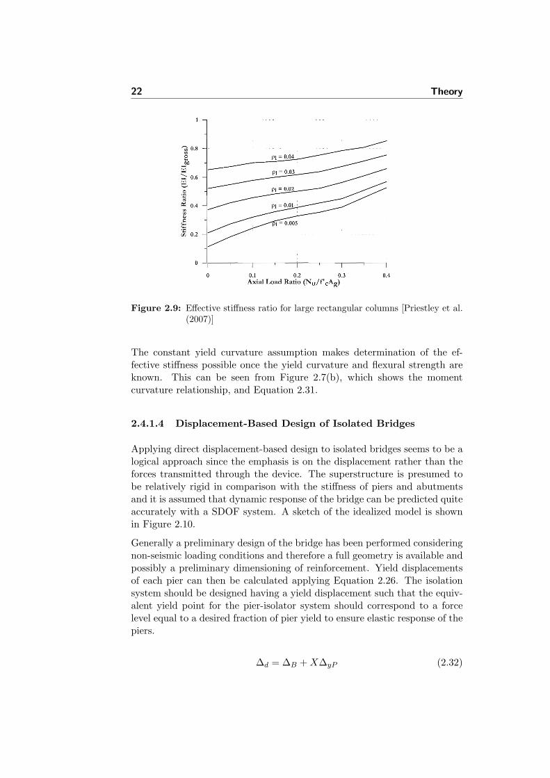
A design procedure flowchart is presented in Figure 2.11 and the step bystep procedure is described below.
1. Design displacement should be selected considering the actual displace-ment spectra, as a function of the local seismicity and the functionalrequirements. A crucial issue will be to decide whether it is acceptableto design for a displacement equal to that corresponding to the cornerperiod in the appropriately damped displacement spectrum.
2. Calculate pier yield displacements with Equation 2.26.3. Equivalent viscous damping obtainable from each type of isolation
system varies. First a value typical for the relevant isolation systemmust be assumed.
4. System equivalent stiffness is given with Equation 2.28 and is a func-tion of effective period and effective mass only.
5. Shear distribution between piers determined. It can e.g. be distributedto provide equal shear or equal moment in the piers. The distributioncan calibrated to obtain an optimal solution regarding stiffness of pier-isolator systems.
6. Determine effective stiffness of isolators and piers from Equations 2.38and 2.39.
7. Determine isolator properties (see Section 2.3.1) and compare calcu-lated equivalent viscous damping values with those assumed in step 3.

26 Theory
If the calculated value based on isolator parameters is not equal to theassumed value iteration is needed until a satisfactory result is reached.
8. Equivalent viscous damping for each pier-isolation system is deter-mined from Equation 2.36 based on assumed damping and displace-ment of piers and isolators.
9. Global equivalent viscous damping determined from Equation 2.36 anddistribution determined in step 5.
10. Reduction factor for displacement spectra determined with Equation2.37.
11. Read displacement from reduced displacement spectra. If it is the sameas assumed design displacement value in step 1, the process continues.If not, a few iterations need to be made.
12. Total base shear force and base shear coefficient determined fromEquation 2.29.
13. Distribute base shear and stiffness to piers and spandrel columns ac-cording to assumption made in step 5.
14. Check if force levels and required stiffnesses are acceptable. If so thedesign process is completed but if not some modifications have to bemade. Depending on the force levels it may be best to modify theinitial input parameters or perhaps change the design displacement orshear distribution. Obviously many options are available and this iswhere the experience of the designer comes in handy.
2.4 Performance Based Design 27
1. Determine design displacement Δd
Initial input parameters: Column dimensions, inertia mass, material properties and design spectra.
2. Calculate pier yield displacements
3. Assume equivalent viscous damping of isolators and force level for design of piers
8. Calculate equivalent viscous damping of each pier-isolator system
9. Calculate global equivalent viscous system damping
10. Calculate damping reduction factor
11. Read displacement from reduced displacement spectra. Is it the same
as design displacement?
12. Calculate total base shear force
13. Distribute base shear and stiffness to piers and spandrel columns.
Calculate section forces in piers.
5. Calculate stiffness of each pier-isolation system
6. Calculate effective stiffness of isolators and piers
4. Calculate system equivalent stiffness
7. Determine isolator properties. Does equivalent viscous damping of isolator
agree with assumed value?
14. Are force levels acceptable?
Finished
YES
NO
YES
NO
YES
Figure 2.11: Flowchart for the displacement-based design for isolated structures
28 Theory
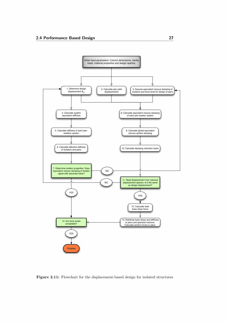
2.4.1.5 Comparison With Force-based Design Approach
It was shown in Section 2.4.1.4 that considering, as basic design parameters,the deck, isolators and pier displacement capacities and demands lead toa simple and effective design approach which only requires the applicationof capacity design principles to protect piers. To illustrate the conceptualdifference between force-based design and direct displacement-based design,simple flowcharts are provided in Figure 2.12. Step by step guides are givenbelow.
1. Period of vibration and damper ductility chosen
1. Design displacement chosen which gives period of vibration
2. Yield displacement of piers and isolator displacement determined
3. System equivalent damping calculated
4. Base shear distributed and required stiffness of piers and isolators obtained
3. Base shear read from acceleration spectrum.
4. Base shear distributed based on assumed stiffness. Pier displacements calculated.
2. Equivalent damping calculated
5. Effective displacement of isolators determined and devices designed
Force-based approach Direct Displacement-based approach
5. Piers and isolators designed to achieve desired response
Figure 2.12: Simple flowcharts for force-based and direct displacement-based de-sign of isolated structures
Force-based Design:
1. Desired period of vibration and acceptable ductility of dampers chosen,T and µd
2. Equivalent damping of system ζeq calculated neglecting pier responsecontribution
3. Design base shear Vbase read from acceleration spectrum with T andζeq
4. Base shear distributed to pier-isolator systems and pier displacementscalculated based on assumed stiffness independent of strength. Pierdisplacements calculated.
5. Effective displacement of each pier-isolator system is ∆e = VuKe
. Isola-tion devices can then be designed.

2.5 Methods of Analysis 29
Direct Displacement-based Design:
1. Choose design displacement ⇒ T2. Calculate yield displacement of piers ⇒ obtain isolator displacements3. System equivalent damping calculated including pier response contri-
bution4. Distribute forces ⇒ obtain required stiffness of piers and isolators5. Design piers and isolators to achieve the desired response
In force-based design the period of vibration and acceptable damping isarbitrarily chosen and will most likely need iteration. Pier displacementscalculated in step 4 are based on assumed stiffness independent of strength.Subsequently the isolator effective displacement is determined from the pierdisplacements and total effective displacement. The procedure is repeatedto convergence if the resulting system should be technically unacceptableor if the assumed ductility differs from the resulting ductility. From theabove it is clear that using this approach does not provide the designer withthe same level of control of the total structural response as in the directdisplacement-based design. The end result might nevertheless be the same,although unlikely.
2.5 Methods of Analysis
Two numerical methods were used for the seismic analysis of the bridge: Re-sponse spectrum analysis and nonlinear time history analysis. These meth-ods are described below. In addition to the seismic analysis methods, staticanalysis was performed to calculate the stresses and deformations of thebridge from non-seismic loading.
The response quantities of interest for the bridge system under considera-tion are: (1) base shear and section forces, (2) relative displacement of thebearings at the abutments and piers for the isolated bridge. Section forcesof structural elements provide an insight in the loaded state of the bridgeand the relative displacements of the bearings are crucial from the designpoint of view of the isolation system and expansion joints.
The following assumptions are made for the earthquake analysis of thebridges under consideration:
1. The bridge deck, piers and arch are assumed to remain in the elasticstate during the earthquake excitation in the base isolated bridge. Thisis a reasonable assumption, as the isolation system is designed suchthat it protects the structural elements by making sure they remain inthe elastic range.
2. The deck of the bridge is straight and is supported at discrete locations

30 Theory
along its longitudinal axis by cross diaphragms. Also the abutmentsof the bridge are assumed to be rigid.
3. The bridge piers and spandrel columns are assumed to be rigidly fixedat the foundation level and on the arch.
4. Two simultaneous horizontal components of earthquake ground mo-tion are considered in the longitudinal and transverse directions of thebridge as well as a vertical component.
5. The stiffness contribution of nonstructural elements such as curbs,parapet walls, and the wearing coat is neglected. However, their massproducing the inertial forces is considered.
6. The bridge is founded on firm rock, and the earthquake excitation isperfectly correlated at all of the supports.
7. The lead rubber bearings are isotropic, implying the same dynamicproperties in two orthogonal directions.
2.5.1 Response Spectrum Analysis
The response spectrum analysis is a procedure for dynamic analysis of astructure subjected to earthquake excitation, but it reduces the problemto a series of static analysis. The response spectrum analysis uses the vi-bration properties of the structure (natural frequencies, natural modes andmodal damping ratios) and the dynamic characteristics of the ground motionthrough its response spectrum. Time history calculations are not necessarysince the calculations have been made in developing the earthquake responsespectrum or in the case of a smooth design spectrum, the properties havebeen characterized by the spectrum.
The exact peak response of each mode can be obtained from the earthquakeresponse spectrum and subsequently the modal responses are combined usinga suitable modal combination rule. The result is not exact in the sense thatis not identical to the response history analysis. It is however considered ac-curate enough for structural design applications [Chopra (2007)]. The resultof a response spectrum analysis using the response spectrum from a groundmotion is typically different from that which would be calculated directlyfrom a linear dynamic analysis using the same ground motion directly, sincephase information is lost in the process of generating the response spectrum.
Several methods have been proposed to combine the modal responses to de-termine the peak value of the total response. A discussion of the proposedmethods is not provided here, but the interested reader is referred to e.g.[Chopra (2007)]. It is not possible to simply add up the modal responsessince they attain their peaks at different time instants and the combinedresponse attains its peak at yet at different instant. Hence, approximationsmust be introduced in combining the peak modal response because no infor-
2.5 Methods of Analysis 31
mation is available as to when these peak modal values occur. The CompleteQuadratic Combination (CQC) rule is widely used and considered to yieldsatisfactory results and is therefore used in the work presented herein. Thetotal peak response, r0, is calculated with
r0 ≈
(N∑i=1
N∑n=1
ρinriorno
)12
(2.41)
where rio and rno are the responses of modes i and n respectively and ρinis the correlation coefficient for modes i and n. The correlation coefficientvaries between 0 and 1 and ρin = 1 for i = n. The correlation coefficient isgiven with (according to Der Kiureghian [Chopra (2007)])
ρin =8√ζiζn(ζi + βinζn)β
32in
(1− β2in)2 + 4ζiζnβin(1 + β2
in) + 4(ζ2i + ζ2
n)β2in
(2.42)
where βin is the ratio between the angular frequency of modes i and n,βin = ωi
ωn, and ζi and ζn are the damping values of modes i and n respectively.
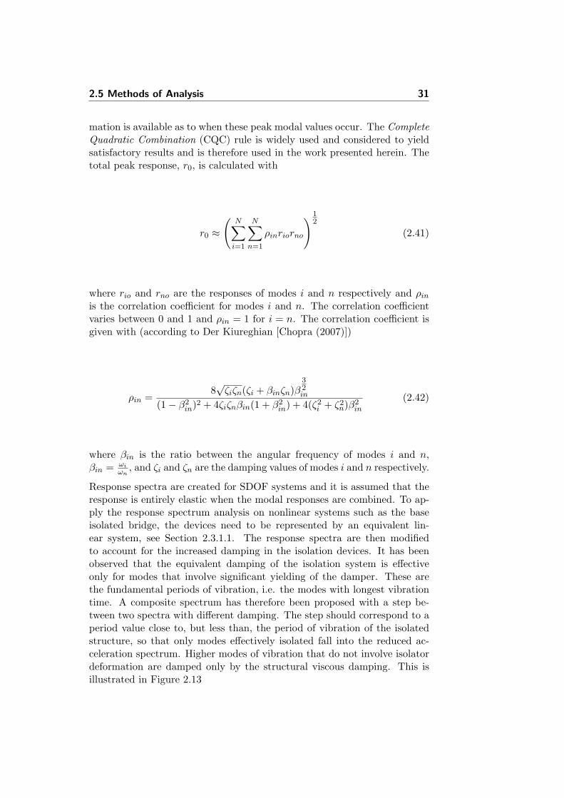
Response spectra are created for SDOF systems and it is assumed that theresponse is entirely elastic when the modal responses are combined. To ap-ply the response spectrum analysis on nonlinear systems such as the baseisolated bridge, the devices need to be represented by an equivalent lin-ear system, see Section 2.3.1.1. The response spectra are then modifiedto account for the increased damping in the isolation devices. It has beenobserved that the equivalent damping of the isolation system is effectiveonly for modes that involve significant yielding of the damper. These arethe fundamental periods of vibration, i.e. the modes with longest vibrationtime. A composite spectrum has therefore been proposed with a step be-tween two spectra with different damping. The step should correspond to aperiod value close to, but less than, the period of vibration of the isolatedstructure, so that only modes effectively isolated fall into the reduced ac-celeration spectrum. Higher modes of vibration that do not involve isolatordeformation are damped only by the structural viscous damping. This isillustrated in Figure 2.13
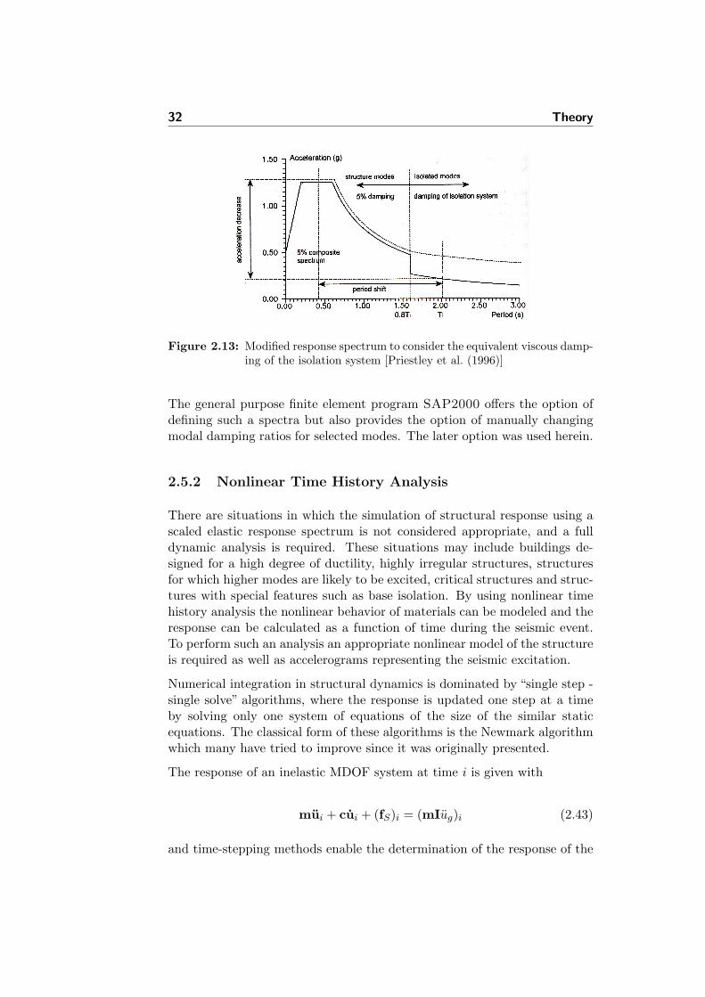
32 Theory
Figure 2.13: Modified response spectrum to consider the equivalent viscous damp-ing of the isolation system [Priestley et al. (1996)]
The general purpose finite element program SAP2000 offers the option ofdefining such a spectra but also provides the option of manually changingmodal damping ratios for selected modes. The later option was used herein.
2.5.2 Nonlinear Time History Analysis
There are situations in which the simulation of structural response using ascaled elastic response spectrum is not considered appropriate, and a fulldynamic analysis is required. These situations may include buildings de-signed for a high degree of ductility, highly irregular structures, structuresfor which higher modes are likely to be excited, critical structures and struc-tures with special features such as base isolation. By using nonlinear timehistory analysis the nonlinear behavior of materials can be modeled and theresponse can be calculated as a function of time during the seismic event.To perform such an analysis an appropriate nonlinear model of the structureis required as well as accelerograms representing the seismic excitation.
Numerical integration in structural dynamics is dominated by “single step -single solve” algorithms, where the response is updated one step at a timeby solving only one system of equations of the size of the similar staticequations. The classical form of these algorithms is the Newmark algorithmwhich many have tried to improve since it was originally presented.
The response of an inelastic MDOF system at time i is given with
mui + cui + (fS)i = (mIug)i (2.43)
and time-stepping methods enable the determination of the response of the

2.5 Methods of Analysis 33
system at time i+ 1:
mui+1 + cui+1 + (fs)i+1 = (mIug)i+1 (2.44)
Newmark developed a family of time-stepping methods in 1959 based on thefollowing equations [Chopra (2007)]
ui+t = ui + [(1− γ)∆t]ui + (γ∆t)ui+t (2.45)
ui+t = ui + (∆t)ui + [(0.5− β)(∆t)2]ui + [β(∆t)2]ui+t (2.46)
where the parameters γ and β define the variation of acceleration over atime step and determine the stability and accuracy characteristics of themethod. Typical values are γ = 1
2 and 16 ≤ β ≤
14 . In this thesis the average
acceleration algorithm is used which is the Newmark method with γ = 12
and β = 14 .
Damping used in direct integration time history analysis is described withthe damping matrix, c. The damping matrix is defined as being proportionalto mass and stiffness by
c = a0m + a1k (2.47)
This is called Rayleigh damping. The damping ratio for the nth mode ofsuch a system is
ζn =a0
21ωn
+a1
2ωn (2.48)
The coefficients a0 and a1 are determined from specified damping ratios ζiand ζj for mode i and j respectively. It is reasonable to have the samedamping ratio for modes i and j and then the coefficients are given with
a0 = ζ2ωiωjωi + ωj
a1 = ζ2
ωi + ωj(2.49)
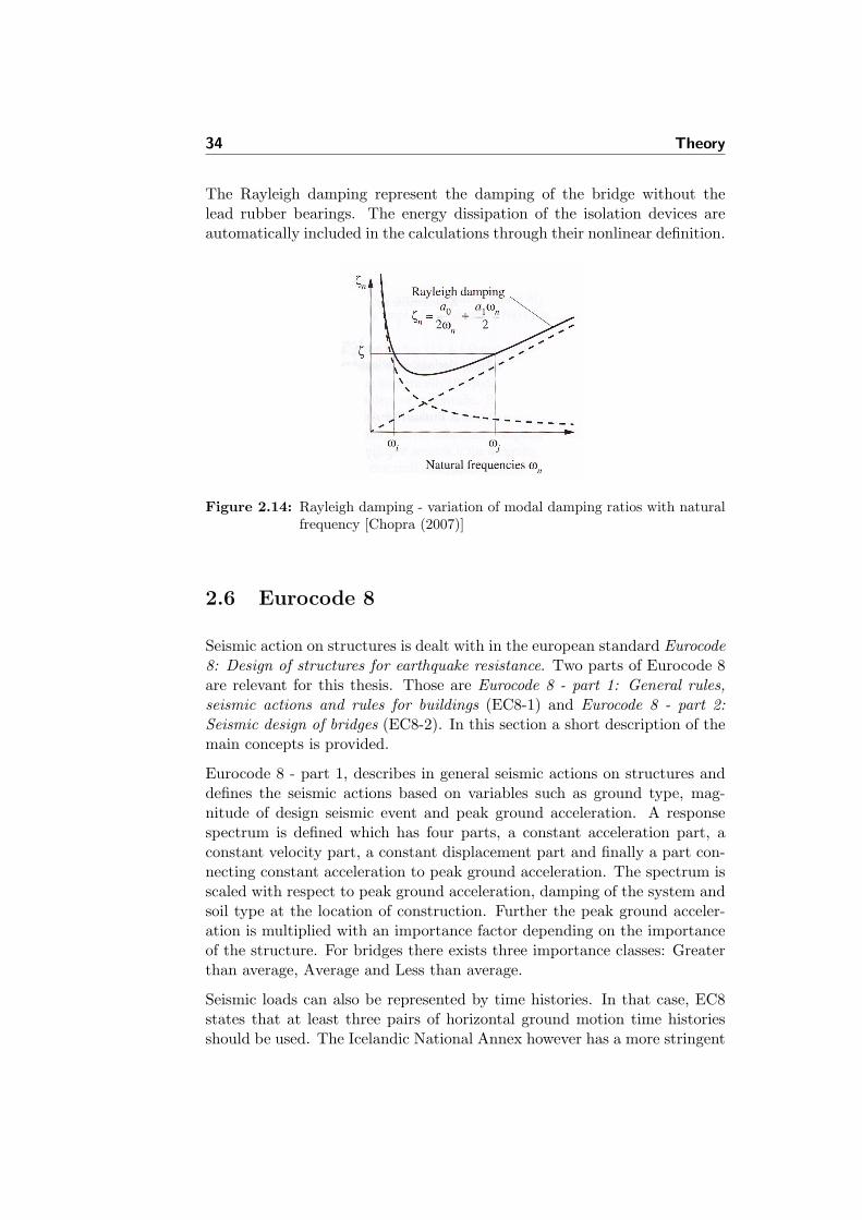
The modes i and j with specified damping ratios should be chosen to ensurereasonable values for the damping ratios in all the modes contributing sig-nificantly to the response. This is illustrated in Figure 2.14. Modes havingangular frequency lower than mode i will be over damped and damping formodes higher than j will increase monotonically with frequency. Dampingfor modes in between i and j will have damping somewhat smaller than ζ.
34 Theory
The Rayleigh damping represent the damping of the bridge without thelead rubber bearings. The energy dissipation of the isolation devices areautomatically included in the calculations through their nonlinear definition.
Figure 2.14: Rayleigh damping - variation of modal damping ratios with naturalfrequency [Chopra (2007)]
2.6 Eurocode 8
Seismic action on structures is dealt with in the european standard Eurocode8: Design of structures for earthquake resistance. Two parts of Eurocode 8are relevant for this thesis. Those are Eurocode 8 - part 1: General rules,seismic actions and rules for buildings (EC8-1) and Eurocode 8 - part 2:Seismic design of bridges (EC8-2). In this section a short description of themain concepts is provided.
Eurocode 8 - part 1, describes in general seismic actions on structures anddefines the seismic actions based on variables such as ground type, mag-nitude of design seismic event and peak ground acceleration. A responsespectrum is defined which has four parts, a constant acceleration part, aconstant velocity part, a constant displacement part and finally a part con-necting constant acceleration to peak ground acceleration. The spectrum isscaled with respect to peak ground acceleration, damping of the system andsoil type at the location of construction. Further the peak ground acceler-ation is multiplied with an importance factor depending on the importanceof the structure. For bridges there exists three importance classes: Greaterthan average, Average and Less than average.
Seismic loads can also be represented by time histories. In that case, EC8states that at least three pairs of horizontal ground motion time historiesshould be used. The Icelandic National Annex however has a more stringent
2.6 Eurocode 8 35
requirement in that it requires at least ten pairs of horizontal ground motiontime histories. Specific rules are given for scaling of the pairs of horizontalmotions independent from the vertical component, so as to render themcompatible to the elastic response spectrum.
Seismic loading for the bridge is described in detail in Section 3.2.4.1 wherethe design spectrum is derived and in Section 3.2.4.2 where artificial timehistories are presented.
Cracked stiffness of concrete members may be taken as equal to one-half ofthe corresponding stiffness of the uncracked elements unless a more accurateanalysis of the cracked elements is performed.
When performing a modal response spectrum analysis the response of allmodes of vibration contributing significantly to the global response shall betaken into account. That is done by either demonstrating that the sum ofthe effective modal masses for the modes taken into account amounts to atleast 90% of the total mass of the structure or by demonstrating that allmodes with effective modal masses greater than 5% of the total mass areconsidered.
Eurocode 8 - part 2, is specific for bridges and has special section dedicatedto seismically isolated bridges. EC8-2 has two basic requirements for designof bridges, the first being that the bridge should retain its structural integrityand adequate residual resistance, although at some parts of the bridge con-siderable damage may occur. The bridge should be damage-tolerant, i.e.those parts of the bridges susceptible to damage, by their contribution toenergy dissipation during the design seismic event, should be designed insuch a manner as to ensure that, following the seismic event, the structurecan sustain the actions from emergency traffic, and inspections and repaircan be performed easily. The second basic requirement is the minimizationof damage during earthquakes with a high probability of occurrence. In sucha case only secondary components and those parts of the bridge intended tocontribute to energy dissipation during the design life of the bridge shouldincur minor damage during earthquakes with a high probability of occur-rence. The non-collapse requirement for bridges under the design seismicevent is more stringent than the relevant requirement for buildings, as itcontains the continuation of emergency traffic.
If the bridge being considered is long, accounting for spatial variability maybe required. The distance beyond which ground motions may be considereduncorrelated is Lg = 600m for ground type A (Bedrock). Accounting forspatial variability is required for bridges with continuous deck when eitherthe bridge length exceeds Lg/1.5 or when more than one ground type cor-respond to the bridge supports. The bridge considered in this thesis is wellbelow the distance founded on bedrock. Hence no consideration was made

36 Theory
on spatial variability.
Three analysis methods for seismically isolated bridges are allowed:
1. Fundamental mode spectrum analysis2. Multi-mode spectrum analysis3. Time history analysis
Specific conditions need to be fulfilled in order to apply the first two methodswhereas the third method can be applied to all seismically isolated bridges.Fundamental mode spectrum analysis can be applied when all the followingconditions are met (in addition to general conditions for fundamental modespectrum analysis):
1. Distance to nearest know seismically active fault exceeds 10 km2. Ground conditions are of type A, B, C or E3. Effective damping < 30%4. Force-displacement relation of the isolation units in each direction is
essentially independent from the rate of loading, magnitude of concur-rent vertical load and horizontal load in transverse direction
5. Effective stiffness of the isolating system at the design displacement isat least equal to 1
3 of the stiffness at 15 of the design displacement
Multi-mode spectrum analysis can be applied when the conditions 2-5 arefulfilled.
In a response spectrum analysis the damping of the isolation system shouldbe used for appropriate modes only. Other modes should be assigned damp-ing of the nonisolated system. This is not explained any further but dividingthe spectrum into two parts as described in Section 2.5.1 is meant to coverthis.
The normal design properties of all isolator units should be assessed bymeans of special prototype tests. Excepted from this rule are normal elas-tomeric bearings, for which normal design properties and design rules aredefined by the code. Also excepted are flat siding bearings, as long as theircontribution to the damping of the isolating system is ignored.
2.7 Ultimate Strength of Elements
When evaluating the seismic response of the bridge the following calcula-tions methods were used to estimate the ultimate strength of elements. Theultimate strength was compared to the results of the FE-analyses.
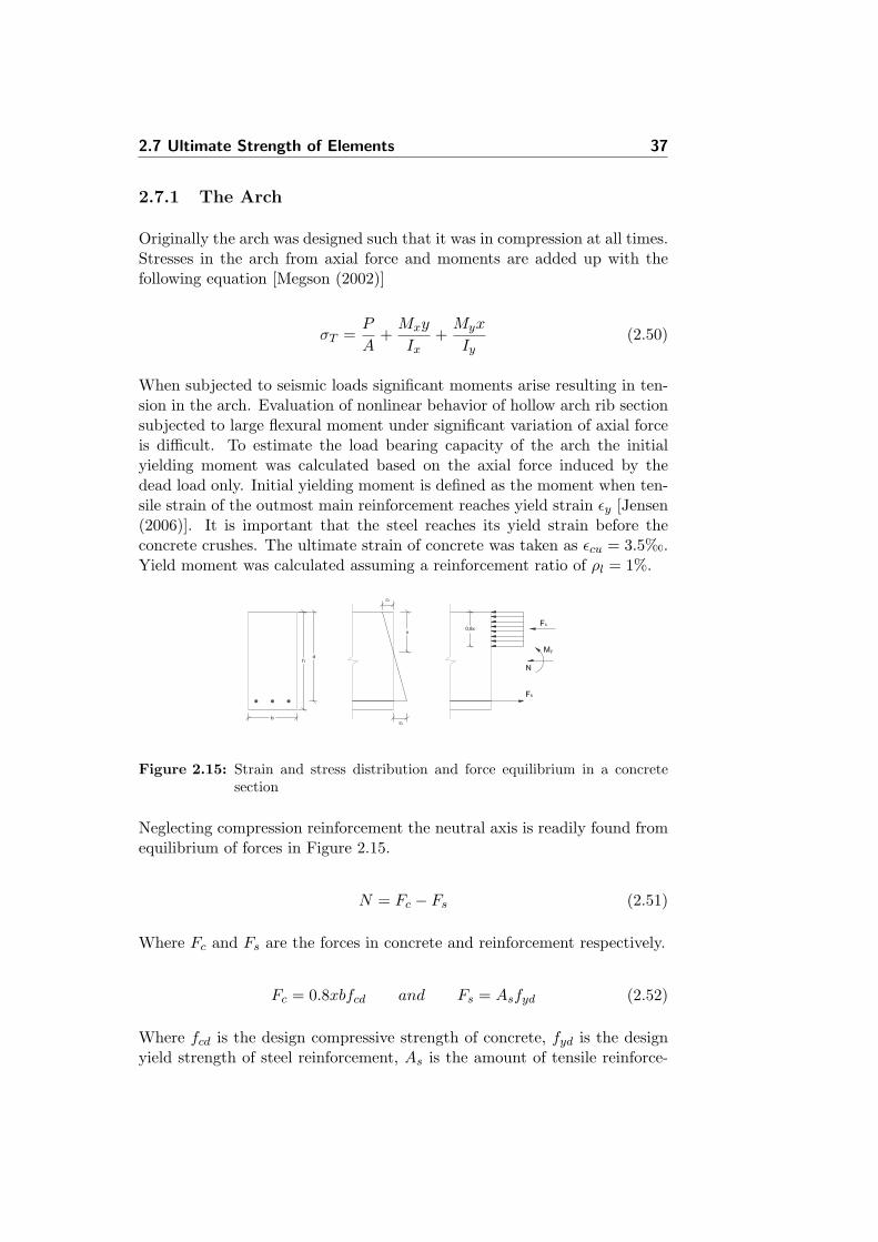
2.7 Ultimate Strength of Elements 37
2.7.1 The Arch
Originally the arch was designed such that it was in compression at all times.Stresses in the arch from axial force and moments are added up with thefollowing equation [Megson (2002)]
σT =P
A+Mxy
Ix+Myx
Iy(2.50)
When subjected to seismic loads significant moments arise resulting in ten-sion in the arch. Evaluation of nonlinear behavior of hollow arch rib sectionsubjected to large flexural moment under significant variation of axial forceis difficult. To estimate the load bearing capacity of the arch the initialyielding moment was calculated based on the axial force induced by thedead load only. Initial yielding moment is defined as the moment when ten-sile strain of the outmost main reinforcement reaches yield strain εy [Jensen(2006)]. It is important that the steel reaches its yield strain before theconcrete crushes. The ultimate strain of concrete was taken as εcu = 3.5‰.Yield moment was calculated assuming a reinforcement ratio of ρl = 1%.
Figure 2.15: Strain and stress distribution and force equilibrium in a concretesection
Neglecting compression reinforcement the neutral axis is readily found fromequilibrium of forces in Figure 2.15.
N = Fc − Fs (2.51)
Where Fc and Fs are the forces in concrete and reinforcement respectively.
Fc = 0.8xbfcd and Fs = Asfyd (2.52)
Where fcd is the design compressive strength of concrete, fyd is the designyield strength of steel reinforcement, As is the amount of tensile reinforce-
38 Theory
ment and b and x are as defined in Figure 2.15. The yield moment is foundby moment equilibrium, here taken about the tension reinforcement.
My = Fc
(d− 0.8x
2
)−N
(d− h
2
)(2.53)
2.7.2 Shear Capacity
Shear capacity was calculated according to Eurocode 2 (EN1992-1-1:2004)with the following equation
VRd,s =Aswszfywdcot(θ) (2.54)
where Asw is the cross-sectional area of the shear reinforcement, s is thespacing of stirrups and fywd is the design yield strength of the shear re-inforcement, z is the inner lever arm and θ is the angle between concretecompression struts and the main tension chord. The maximum allowableshear resistance acquired from Equation 2.54 is bounded by
VRd,max =αcwbwzµ1fcdcot(θ) + tan(θ)
(2.55)
Where µ1 is a strength reduction factor for concrete cracked in shear and αcwis a coefficient taking account of the state of the stress in the compressionchord. Equation 2.55 ensures that no crushing occurs in the compressionchord.
2.7.3 Piers and Spandrel Columns
Load bearing capacity of piers and spandrel columns is calculated by con-struction N-M interaction diagrams for uniaxial moment. The diagram issimplified by calculating only three points.
A Pure compression. Ultimate compressive strength of the piers andspandrel columns
B Balanced failure. Steel and concrete reach ultimate strains and failsimultaneously
C Pure moment. Steel yields before concrete fails in compression. Mo-ment capacity with no normal force
Forces are extracted from the FE-program and plotted on a N-M diagramfor the respective pier or spandrel column.

2.7 Ultimate Strength of Elements 39
Figure 2.16: Simplified N-M interaction diagram for uniaxial bending
2.7.4 Bridge Deck
The loaded state of the bridge deck was evaluated based on calculated mo-ment and shear capacity. Shear capacity is calculated as in Section 2.7.2 andthe moment capacity is calculated by viewing the box girder as a series ofT-beams with effective flange width estimated with methods from Eurocode2.
Moment capacity is then calculated with the same method as for the archin Section 2.7.1 and omitting the normal force N from Equations 2.51 and2.53.


Chapter 3
The Bridge and Applied Load
In this chapter the analyzed bridges are described as well as the appliedload. The bridges do not exist in reality but they are assumed to be locatedin the south of Iceland.
The chapter starts with a description of the original bridge and its struc-tural elements followed by a description of the lead rubber bearings usedin the base isolated bridge. Subsequently the results of modal analysis arepresented for the original and base isolated bridge.
In Section 3.2 the applied load is described.
3.1 The Bridge
The bridge analyzed is a reinforced concrete arch bridge with the arch po-sitioned below the bridge deck. The arch has a span of 100m and a riseof 22.3m, resulting in a span-to-rise ratio of 4.48. The superstructure iscontinuous with a total span of L = 9× 20m = 180m.
In the original bridge, expansion joints are introduced immediately outsidethe main spandrel columns resting on the arch foundations. These columnsare therefore designed to be stronger than the others and able to transmitthe horizontal forces from the deck to the foundation. The horizontal forcesconsidered in the original design were mainly due to thermal actions (ex-pansion and contraction of the concrete) but also due to deformation of thestructure.

42 The Bridge and Applied Load
Figure 3.1: Three dimensional view of the bridge
3.1.1 Structural Elements
The arch is fixed and of double cell box type cross section with constantheight and width of 1.6m and 8.5m respectively. The arch cross section isuniform along the length with 0.2m thick top and bottom chords and bothinner and outer webs are 0.2m thick.
To distinguish between the columns resting on ground and the ones restingon the arch the first group is termed piers and the latter spandrel columns.The term columns covers both groups. Four double spandrel columns arepositioned symmetrically on the arch, positioned at 10m and 30m from thearch crown respectively. Diaphragms are placed inside the arch under span-drel columns. The spandrel columns resting on the arch foundation aresomewhat bigger than the others and termed main spandrel columns to dis-tinguish them from the others. Outside the arch two double piers supportthe approach span. The main spandrel columns have a square hollow crosssection with outer dimensions 1.8m×1.8m and wall thickness 0.25m whereasthe other columns have a rectangular hollow section with outer dimensions1.0m × 0.7m and wall thickness 0.20m. In the original bridge the columnsare fixed at their lower end and monolithically connected to the bridge deck.This is by far the most convenient construction method and the results ob-tained from statical analysis indicated that there was no need for bearingsover the short columns. Column heights vary and are approximately equalto (from the abutment to the crown): 6.1m, 26.1m, 11.8m and 4.5m. Thebridge is symmetrical so only half of the columns are listed.
The bridge deck is made of non-prestressed concrete and is placed entirelyabove the arch. It is a continuous structure supported partly by piers andpartly by spandrel columns resting on the arch with a span length of 20m.The deck section is a closed three-cell box-girder with constant height 1.8mand a total width of 17.5m. External and internal webs have a thickness

3.1 The Bridge 43
Figure 3.2: General cross section in bridge
of 0.25m and 0.35m, respectively. Top and bottom slab have a thickness of0.25m and 0.24m, respectively.
The abutments are stub abutments and there are no bearings or expan-sion joints placed at the abutments in the original bridge. The bridge deckis monolithically connected to the abutments making construction easier.Foundations are cast-in-situ direct foundations transferring moment and ax-ial force to the bedrock.
3.1.2 Material Properties
Concrete is a very suitable material for an arch structure since it has a highcompressive strength but an unreliable tensile strength. When designing theshape of the arch the goal is to keep it in compression at all times and try tolimit the bending moments. If the arch is made of concrete it makes senseto make the piers, spandrel columns and bridge deck of concrete as well.Material properties used in calculations are as follows
Compressive strength of concrete fck = 50 MPaPartial factor for concrete γc = 1.5Self weight of concrete (incl. rebars) γconc = 25 kN/m3
Modulus of Elasticity Ecm = 37.000 MPaYield strength of rebars fy = 500 MPaPartial factor for rebars γs = 1.15
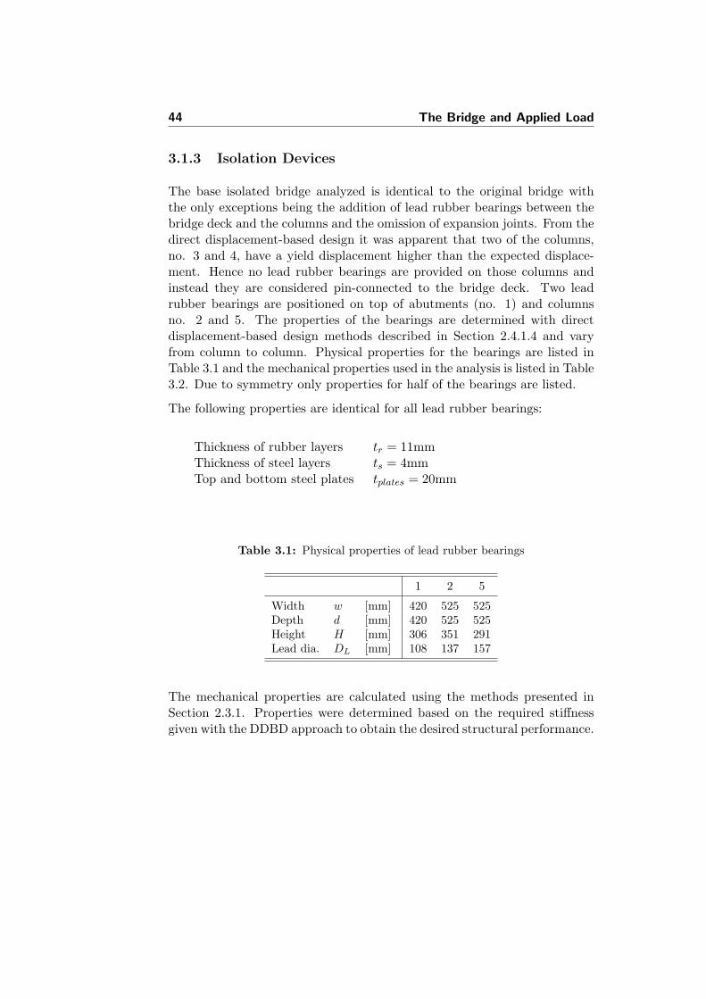
44 The Bridge and Applied Load
3.1.3 Isolation Devices
The base isolated bridge analyzed is identical to the original bridge withthe only exceptions being the addition of lead rubber bearings between thebridge deck and the columns and the omission of expansion joints. From thedirect displacement-based design it was apparent that two of the columns,no. 3 and 4, have a yield displacement higher than the expected displace-ment. Hence no lead rubber bearings are provided on those columns andinstead they are considered pin-connected to the bridge deck. Two leadrubber bearings are positioned on top of abutments (no. 1) and columnsno. 2 and 5. The properties of the bearings are determined with directdisplacement-based design methods described in Section 2.4.1.4 and varyfrom column to column. Physical properties for the bearings are listed inTable 3.1 and the mechanical properties used in the analysis is listed in Table3.2. Due to symmetry only properties for half of the bearings are listed.
The following properties are identical for all lead rubber bearings:
Thickness of rubber layers tr = 11mmThickness of steel layers ts = 4mmTop and bottom steel plates tplates = 20mm
Table 3.1: Physical properties of lead rubber bearings
1 2 5
Width w [mm] 420 525 525Depth d [mm] 420 525 525Height H [mm] 306 351 291Lead dia. DL [mm] 108 137 157
The mechanical properties are calculated using the methods presented inSection 2.3.1. Properties were determined based on the required stiffnessgiven with the DDBD approach to obtain the desired structural performance.
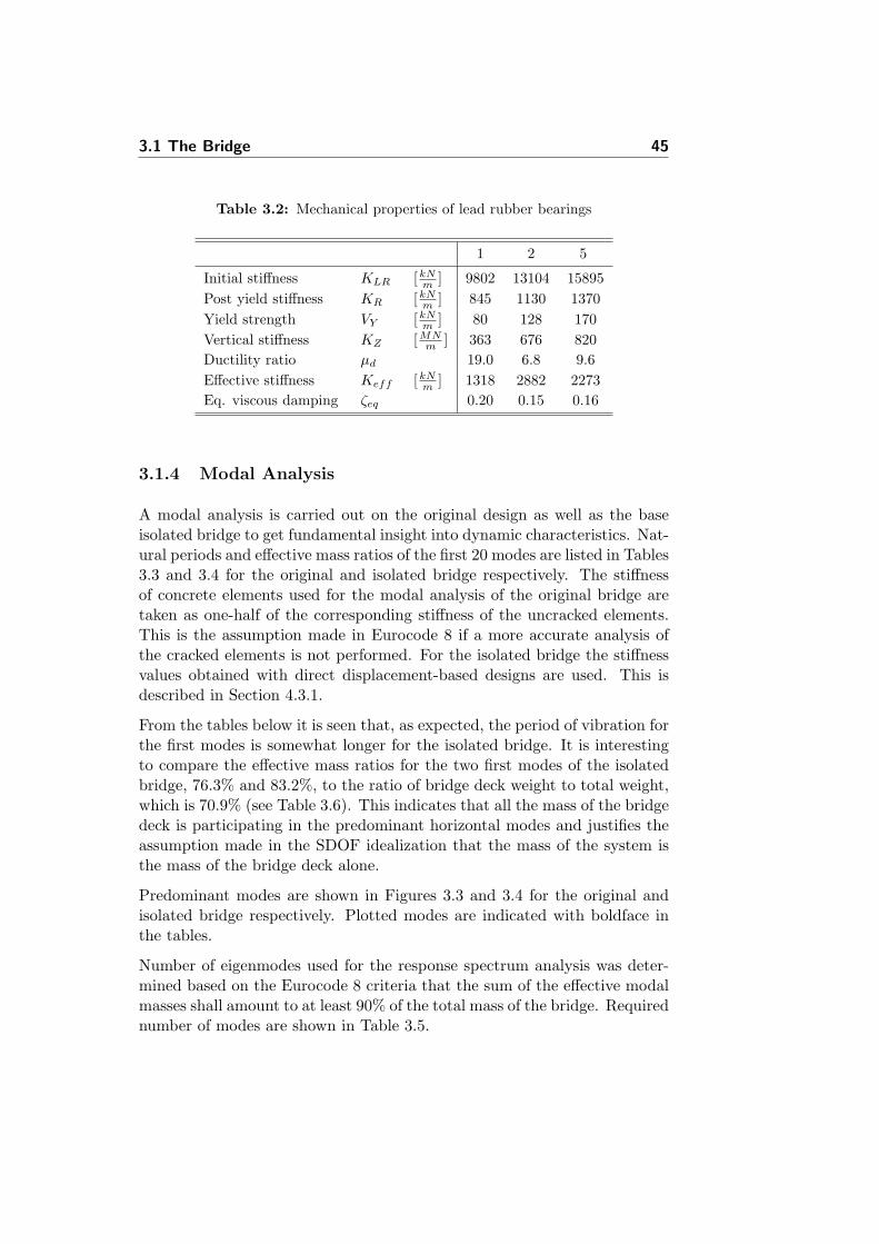
3.1 The Bridge 45
Table 3.2: Mechanical properties of lead rubber bearings
1 2 5
Initial stiffness KLR [kNm ] 9802 13104 15895
Post yield stiffness KR [kNm ] 845 1130 1370
Yield strength VY [kNm ] 80 128 170
Vertical stiffness KZ [MNm ] 363 676 820
Ductility ratio µd 19.0 6.8 9.6Effective stiffness Keff [kN
m ] 1318 2882 2273Eq. viscous damping ζeq 0.20 0.15 0.16
3.1.4 Modal Analysis
A modal analysis is carried out on the original design as well as the baseisolated bridge to get fundamental insight into dynamic characteristics. Nat-ural periods and effective mass ratios of the first 20 modes are listed in Tables3.3 and 3.4 for the original and isolated bridge respectively. The stiffnessof concrete elements used for the modal analysis of the original bridge aretaken as one-half of the corresponding stiffness of the uncracked elements.This is the assumption made in Eurocode 8 if a more accurate analysis ofthe cracked elements is not performed. For the isolated bridge the stiffnessvalues obtained with direct displacement-based designs are used. This isdescribed in Section 4.3.1.
From the tables below it is seen that, as expected, the period of vibration forthe first modes is somewhat longer for the isolated bridge. It is interestingto compare the effective mass ratios for the two first modes of the isolatedbridge, 76.3% and 83.2%, to the ratio of bridge deck weight to total weight,which is 70.9% (see Table 3.6). This indicates that all the mass of the bridgedeck is participating in the predominant horizontal modes and justifies theassumption made in the SDOF idealization that the mass of the system isthe mass of the bridge deck alone.
Predominant modes are shown in Figures 3.3 and 3.4 for the original andisolated bridge respectively. Plotted modes are indicated with boldface inthe tables.
Number of eigenmodes used for the response spectrum analysis was deter-mined based on the Eurocode 8 criteria that the sum of the effective modalmasses shall amount to at least 90% of the total mass of the bridge. Requirednumber of modes are shown in Table 3.5.

46 The Bridge and Applied Load
Table 3.3: Modal analysis results of original bridge
Effective mass ratio
Mode Period, T [s] Longitudinal [%] Transverse [%] Vertical [%]
1 1.084 0.0 78.2 0.02 0.889 30.5 0.0 0.03 0.711 0.0 0.0 0.04 0.498 19.7 0.0 0.05 0.374 0.0 0.0 0.76 0.335 0.0 0.8 0.07 0.242 0.0 0.0 49.08 0.212 0.3 0.0 0.09 0.166 0.0 5.4 0.010 0.157 0.0 0.0 0.011 0.149 0.0 0.0 1.912 0.138 2.7 0.0 0.013 0.137 0.0 0.0 0.714 0.132 0.1 0.0 0.015 0.132 0.0 0.0 0.116 0.120 0.0 0.0 0.017 0.118 1.1 0.0 0.018 0.115 0.0 0.0 2.019 0.107 0.0 0.0 0.720 0.106 3.8 0.0 0.0
Figure 3.3: Predominant modeshapes of the original bridge in the longitudinal,transverse and vertical direction respectively
Figure 3.4: Predominant modeshapes of the isolated bridge in the longitudinal,transverse and vertical direction respectively

3.1 The Bridge 47
Table 3.4: Modal analysis results of isolated bridge
Effective mass ratio
Mode Period, T [s] Longitudinal [%] Transverse [%] Vertical [%]
1 2.502 76.3 0.0 0.02 1.586 0.0 83.2 0.03 1.542 0.0 0.0 0.04 0.699 0.0 0.2 0.05 0.685 2.3 0.0 0.06 0.481 0.0 6.4 0.07 0.372 0.0 0.0 2.58 0.282 0.0 0.0 0.09 0.245 0.0 0.0 41.910 0.218 0.0 0.0 0.011 0.217 1.8 0.0 0.012 0.210 0.9 0.0 0.013 0.196 0.0 0.0 0.014 0.160 0.0 0.1 0.015 0.152 0.0 0.0 1.716 0.148 0.0 0.0 16.617 0.148 0.0 0.0 0.018 0.138 0.8 0.0 0.019 0.130 0.0 0.0 2.220 0.125 1.1 0.0 0.0
Table 3.5: Required number of modes to reach an effective mass ratio of 90%
Original Isolated
Transverse 27 28Longitudinal 47 46Vertical 58 47
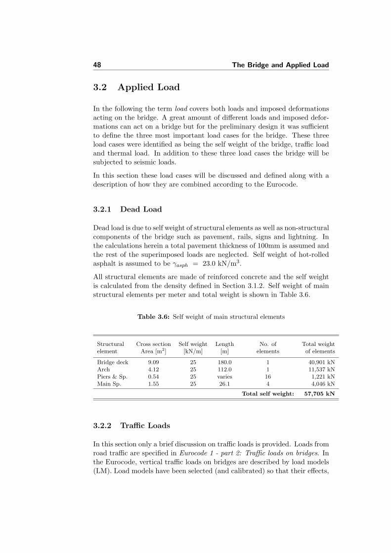
48 The Bridge and Applied Load
3.2 Applied Load
In the following the term load covers both loads and imposed deformationsacting on the bridge. A great amount of different loads and imposed defor-mations can act on a bridge but for the preliminary design it was sufficientto define the three most important load cases for the bridge. These threeload cases were identified as being the self weight of the bridge, traffic loadand thermal load. In addition to these three load cases the bridge will besubjected to seismic loads.
In this section these load cases will be discussed and defined along with adescription of how they are combined according to the Eurocode.
3.2.1 Dead Load
Dead load is due to self weight of structural elements as well as non-structuralcomponents of the bridge such as pavement, rails, signs and lightning. Inthe calculations herein a total pavement thickness of 100mm is assumed andthe rest of the superimposed loads are neglected. Self weight of hot-rolledasphalt is assumed to be γasph = 23.0 kN/m3.
All structural elements are made of reinforced concrete and the self weightis calculated from the density defined in Section 3.1.2. Self weight of mainstructural elements per meter and total weight is shown in Table 3.6.
Table 3.6: Self weight of main structural elements
Structural Cross section Self weight Length No. of Total weightelement Area [m2] [kN/m] [m] elements of elements
Bridge deck 9.09 25 180.0 1 40,901 kNArch 4.12 25 112.0 1 11,537 kNPiers & Sp. 0.54 25 varies 16 1,221 kNMain Sp. 1.55 25 26.1 4 4,046 kN
Total self weight: 57,705 kN
3.2.2 Traffic Loads
In this section only a brief discussion on traffic loads is provided. Loads fromroad traffic are specified in Eurocode 1 - part 2: Traffic loads on bridges. Inthe Eurocode, vertical traffic loads on bridges are described by load models(LM). Load models have been selected (and calibrated) so that their effects,

3.2 Applied Load 49
with dynamic increments taken into account where indicated, represent theeffects of actual traffic.
Loads due to traffic give rise to vertical and horizontal, static and dynamicforces. The dynamic forces are not considered in this preliminary design.The load models for vertical traffic loads are described below.
• Load Model 1 (LM1) Consist of two partial systems, an axle load as atandem system (TS) and uniformly distributed load (UDL). The load appliedis different for each lane and is dependent on the number of lanes. This isillustrated in Figure 3.5 and the magnitude of the loads is listed in Table 3.7.This load model covers most of the effects of the traffic of lorries and carsand should be used for general and local verifications.
• Load Model 2 (LM2) A single axle load applied on specific tyre contactareas which covers the dynamic effects of the normal traffic on short structuralmembers.
• Load Model 3 (LM3) A load model for special vehicles who need specialattention. Applied as a set of assemblies of axle loads representing the ve-hicles. This could for instance be heavy industry transportation or militaryrelated vehicles. Intended for local verifications.
• Load Model 4 (LM4) A crowd loading applied as an uniformly distributedload. This is relevant for bridges located in or near towns and intended forgeneral verification only.
For this preliminary design it is assumed that the bridge does not need to bedesigned specifically to special vehicles and only load model 1 is considered.
Table 3.7: LM1: Characteristic values
Location Tandem system Uniformly distributed loadAxle loads Qik[kN ] qik[kN/m2]
Lane no. 1 300 9.0Lane no. 2 200 2.5Lane no. 3 100 2.5Other lanes 0 2.5
Remaining area (qrk) 0 2.5
General effects can be calculated by replacing each tandem system by a one-axle concentrated load of weight equal to the total weight of the two axels.The value of αQi in Figure 3.5 is taken as 1, which corresponds to a trafficfor which a heavy industrial international traffic is expected (EC1-2).
The simultaneity of the loading systems defined in the Eurocode should betaken into account by considering the groups of loads defined in Table 4.4ain EC1-2, displayed in Figure 3.6.
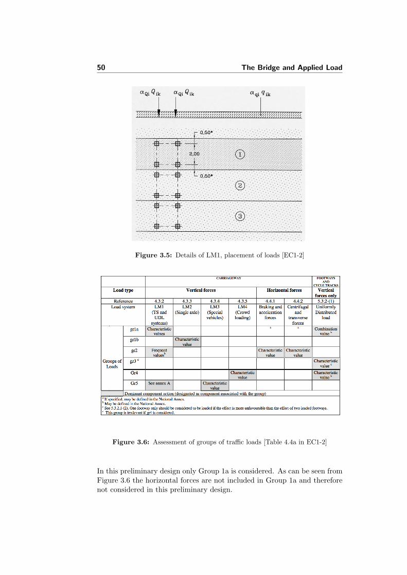
50 The Bridge and Applied Load
Figure 3.5: Details of LM1, placement of loads [EC1-2]
Figure 3.6: Assessment of groups of traffic loads [Table 4.4a in EC1-2]
In this preliminary design only Group 1a is considered. As can be seen fromFigure 3.6 the horizontal forces are not included in Group 1a and thereforenot considered in this preliminary design.
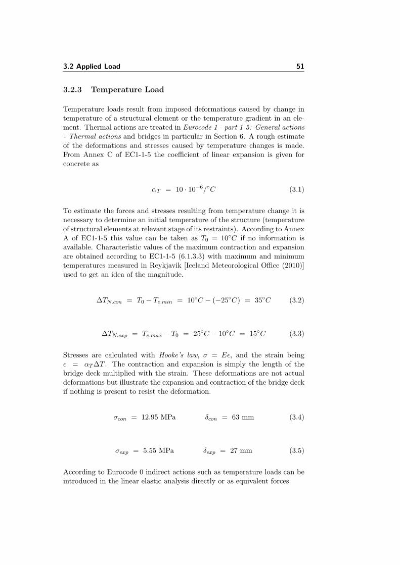
3.2 Applied Load 51
3.2.3 Temperature Load
Temperature loads result from imposed deformations caused by change intemperature of a structural element or the temperature gradient in an ele-ment. Thermal actions are treated in Eurocode 1 - part 1-5: General actions- Thermal actions and bridges in particular in Section 6. A rough estimateof the deformations and stresses caused by temperature changes is made.From Annex C of EC1-1-5 the coefficient of linear expansion is given forconcrete as
αT = 10 · 10−6/◦C (3.1)
To estimate the forces and stresses resulting from temperature change it isnecessary to determine an initial temperature of the structure (temperatureof structural elements at relevant stage of its restraints). According to AnnexA of EC1-1-5 this value can be taken as T0 = 10◦C if no information isavailable. Characteristic values of the maximum contraction and expansionare obtained according to EC1-1-5 (6.1.3.3) with maximum and minimumtemperatures measured in Reykjavik [Iceland Meteorological Office (2010)]used to get an idea of the magnitude.
∆TN.con = T0 − Te.min = 10◦C − (−25◦C) = 35◦C (3.2)
∆TN.exp = Te.max − T0 = 25◦C − 10◦C = 15◦C (3.3)
Stresses are calculated with Hooke’s law, σ = Eε, and the strain beingε = αT∆T . The contraction and expansion is simply the length of thebridge deck multiplied with the strain. These deformations are not actualdeformations but illustrate the expansion and contraction of the bridge deckif nothing is present to resist the deformation.
σcon = 12.95 MPa δcon = 63 mm (3.4)
σexp = 5.55 MPa δexp = 27 mm (3.5)
According to Eurocode 0 indirect actions such as temperature loads can beintroduced in the linear elastic analysis directly or as equivalent forces.

52 The Bridge and Applied Load
3.2.4 Seismic Load
3.2.4.1 The Design Response Spectrum
As mentioned in Chapter 1 the bridge is to be erected in the South IcelandSeismic Zone (SISZ). The design response spectrum is evaluated from thepeak ground acceleration found in the Icelandic National Annex (FS ENV1998-1-1:1994) shown in Figure 3.7. The peak ground acceleration for thearea considered is ag = 0.4g.
Figure 3.7: Horizontal peak acceleration for Iceland [FS ENV 1998-1-1:1994]
In Table 3.8 below the input parameters for the calculation of the designspectra are listed. The soil conditions at bridge construction site is assumedto be bedrock and hence classifies as ground type A according to the Eu-rocode. The bridge is considered to belong to the importance class average.The behavior factor was chosen to be q = 1.2 which is the value to be usedfor limited ductile arches.
Table 3.8: Input to design response spectrum
Ground type AImportance factor γI = 1.0Peak ground acceleration ag = 0.4gBehavior factor q = 1.2

3.2 Applied Load 53
These values serve as input to the calculations on the shape of the horizontaldesign response spectrum which is defined by the following expressions
0 ≤ T ≤ TB : Sd(T ) = agS
[23
+T
TB
(2.5q− 2
3
)]
TB ≤ T ≤ TC : Sd(T ) = agS2.5q
TC ≤ T ≤ TD : Sd(T ) = agS2.5q
[TCT
]
TD ≤ T : Sd(T ) = agS2.5q
[TCTDT 2
]
where T is the vibration period of a linear SDOF system, TB and TC arelimits of the constant spectral acceleration branch, TD is the value definingthe beginning of the constant displacement response range of the spectrumand S is the soil factor. The values of these variables depend on the groundtype and expected surface-wave magnitude. Recommended values for Type1 design response spectrum, ground type A, are listed in Table 3.9 below.
Table 3.9: Parameters for Type 1 design response spectrum
Ground type S TB TC TD
A 1.0 0.15 0.4 2.0
The vertical design response spectra is defined with the same expressionswith the design ground acceleration in the vertical direction, avg replacingag. For Type 1 design spectrum the design ground acceleration in the verticaldirection is taken as avg = 0.9ag.
The horizontal and vertical design spectrum is evaluated in Matlab andshown below in Figures 3.8 and 3.9. The periods of the predominant hori-zontal and vertical modes of the original and isolated bridge are indicatedon the spectra with red and blue diamonds respectively.
As mentioned in Section 2.4.1 the direct displacement-based design usesthe elastic displacement response spectra to determine the target maximumdisplacement and effective period of the structure at maximum response. InFigure 3.10 the 5% damped spectrum is plotted with a solid line and the20% damped with a dotted line.
It is seen that the corner period is Tcorner = 2s and the corresponding

54 The Bridge and Applied Load
Figure 3.8: Horizontal design response spectrum. Predominant horizontal modesindicated with diamonds
Figure 3.9: Vertical design response spectrum. Predominant vertical modes indi-cated with diamonds
displacement based on 5% viscous damping is ∆corner ≈ 200mm. Increaseddamping is shown to produce lower displacement values for constant periods.
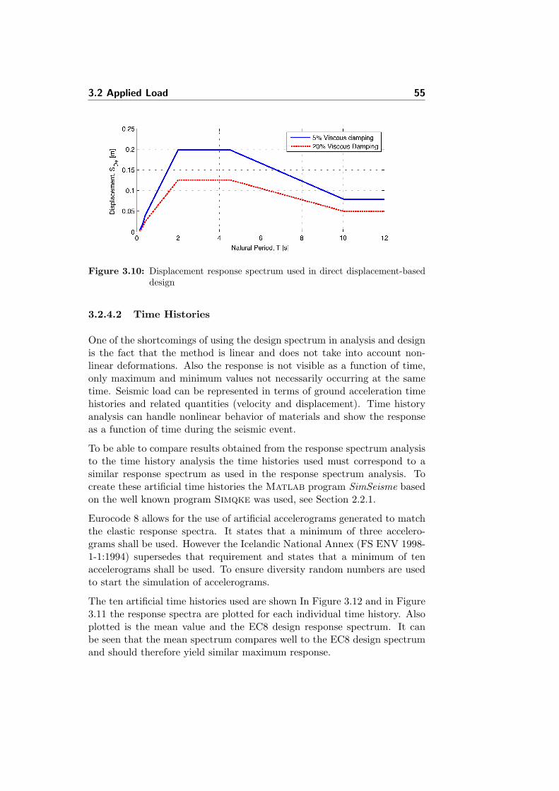
3.2 Applied Load 55
Figure 3.10: Displacement response spectrum used in direct displacement-baseddesign
3.2.4.2 Time Histories
One of the shortcomings of using the design spectrum in analysis and designis the fact that the method is linear and does not take into account non-linear deformations. Also the response is not visible as a function of time,only maximum and minimum values not necessarily occurring at the sametime. Seismic load can be represented in terms of ground acceleration timehistories and related quantities (velocity and displacement). Time historyanalysis can handle nonlinear behavior of materials and show the responseas a function of time during the seismic event.
To be able to compare results obtained from the response spectrum analysisto the time history analysis the time histories used must correspond to asimilar response spectrum as used in the response spectrum analysis. Tocreate these artificial time histories the Matlab program SimSeisme basedon the well known program Simqke was used, see Section 2.2.1.
Eurocode 8 allows for the use of artificial accelerograms generated to matchthe elastic response spectra. It states that a minimum of three accelero-grams shall be used. However the Icelandic National Annex (FS ENV 1998-1-1:1994) supersedes that requirement and states that a minimum of tenaccelerograms shall be used. To ensure diversity random numbers are usedto start the simulation of accelerograms.
The ten artificial time histories used are shown In Figure 3.12 and in Figure3.11 the response spectra are plotted for each individual time history. Alsoplotted is the mean value and the EC8 design response spectrum. It canbe seen that the mean spectrum compares well to the EC8 design spectrumand should therefore yield similar maximum response.
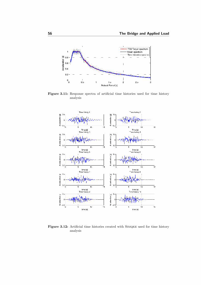
56 The Bridge and Applied Load
Figure 3.11: Response spectra of artificial time histories used for time historyanalysis
Figure 3.12: Artificial time histories created with Simqke used for time historyanalysis
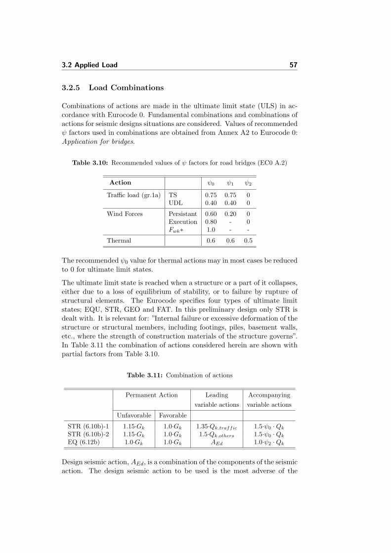
3.2 Applied Load 57
3.2.5 Load Combinations
Combinations of actions are made in the ultimate limit state (ULS) in ac-cordance with Eurocode 0. Fundamental combinations and combinations ofactions for seismic designs situations are considered. Values of recommendedψ factors used in combinations are obtained from Annex A2 to Eurocode 0:Application for bridges.
Table 3.10: Recommended values of ψ factors for road bridges (EC0 A.2)
Action ψ0 ψ1 ψ2
Traffic load (gr.1a) TS 0.75 0.75 0UDL 0.40 0.40 0
Wind Forces Persistant 0.60 0.20 0Execution 0.80 - 0Fwk∗ 1.0 - -
Thermal 0.6 0.6 0.5
The recommended ψ0 value for thermal actions may in most cases be reducedto 0 for ultimate limit states.
The ultimate limit state is reached when a structure or a part of it collapses,either due to a loss of equilibrium of stability, or to failure by rupture ofstructural elements. The Eurocode specifies four types of ultimate limitstates; EQU, STR, GEO and FAT. In this preliminary design only STR isdealt with. It is relevant for: ”Internal failure or excessive deformation of thestructure or structural members, including footings, piles, basement walls,etc., where the strength of construction materials of the structure governs”.In Table 3.11 the combination of actions considered herein are shown withpartial factors from Table 3.10.
Table 3.11: Combination of actions
Permanent Action Leading Accompanyingvariable actions variable actions
Unfavorable Favorable
STR (6.10b)-1 1.15·Gk 1.0·Gk 1.35·Qk.traffic 1.5·ψ0 ·Qk
STR (6.10b)-2 1.15·Gk 1.0·Gk 1.5·Qk.others 1.5·ψ0 ·Qk
EQ (6.12b) 1.0·Gk 1.0·Gk AEd 1.0·ψ2 ·Qk
Design seismic action, AEd, is a combination of the components of the seismicaction. The design seismic action to be used is the most adverse of the

58 The Bridge and Applied Load
following combinations listed in Table 3.12:
Table 3.12: Combinations of components of seismic action
AEx AEy AEz
Quake-X 1.0 0.3 0.3Quake-Y 0.3 1.0 0.3Quake-Z 0.3 0.3 1.0
Where AEx, AEy and AEz are the seismic actions in each direction X,Y andZ respectively.
Mainly two load combinations at the ultimate limit state were consideredin the preliminary design of the original bridge. One had traffic as leadingvariable action and the other had the temperature actions as leading variableaction. They are referred to as ULS-Traffic and ULS-Temp respectively.Seismic combinations are referred to as Quake-X for the combination withthe longitudinal seismic component as the dominating one, Quake-Y for thecombination with the transverse seismic component as the dominating oneand Quake-Z for the combination with the vertical seismic component as thedominating one.
In general seismic action effects need not be combined with action effectsdue to imposed deformations such as temperature variation. However, anexception to that rule is the case of bridges in which the seismic action isresisted by elastomeric laminated bearings. In that case the action effectsdue to imposed deformations shall be accounted for.
Chapter 4
Static and Linear DynamicAnalysis
In this chapter the main results of the response spectrum analysis are pre-sented along with results from static analysis. It starts with a descriptionof the computational model used for analysis with the general purpose fi-nite element program SAP2000, followed by the response of the originalbridge and subsequently the isolated bridge. The chapter concludes withsuggestions for redesign based on the results presented.
Response spectrum analysis was performed by applying seismic loads ob-tained from Eurocode 8 representing the South Iceland Seismic Zone de-fined in Section 3.2.4. Seismic forces are applied in all three directions andcombined with load combinations as described in Section 3.2.5.
4.1 Computational Model
A three dimensional computational model of the bridge with and without thelead rubber bearings was created in SAP2000. Beam elements are used tomodel the structural elements and nonlinear link elements, with equivalentlinear properties for linear analysis, are used to simulate the lead rubberbearings. Link elements connect two joints together and each link elementmay exhibit up to three different types of behavior: linear, nonlinear andfrequency-dependent, according to the types of properties assigned to theelement and the type of analysis being performed. Various types of nonlinearproperties are available but to model the bilinear behavior of the lead rubber

60 Static and Linear Dynamic Analysis
bearings the hysteretic isolator property is used. It is a coupled plasticitymodel available in the SAP2000 program, see [Computers and StructuresInc. (2007)], which is adopted from [Wen (1976)] and [Park et al. (1986)].
SAP2000
SAP2000 v14.0.0 - File:Arch model variable arch (100m) w bearings - RSA - 3-D View - KN, m, C Units
3.31.10 14:03:36
Figure 4.1: Screen shot of computational model from SAP2000
The arch is divided into 150 elements, columns into elements of maximumlength 1m and the bridge deck into elements of maximum length 2m. Thenumber of elements was determined from considerations of the results of themodal analysis. A compromise needs to be made between accuracy of themodel and computational time since the direct integration method used fornonlinear analysis can be very time consuming.
4.2 Original Bridge
The original bridge was not designed for seismic load. In this section theresponse of the bridge to static loads are compared to the response obtainedwith a response spectrum analysis. First the response to static loads ispresented to create a basis for comparison with the response to seismic loadpresented subsequently.
4.2.1 Response to Static Loads
The axial force and bending moment of the arch rib due to the dead loadis shown in Figure 4.2. The axial force and the bending moment due to thedesign load combinations ULS-Traffic and ULS-Temp, which are the mostpredominant in design, are presented as well.
It is seen in Figure 4.2 that the major part of the of the design axial forceis induced by the dead load. A closer look at the results show that approx-imately 83% of the design axial force is induced by the dead load. For the

4.2 Original Bridge 61
Figure 4.2: Axial force and bending moment in arch due to static loads
bending moment the dead load induces approximately 64% of the momentin the arch rib at the point where it reaches its maximum.
Stresses in arch top and bottom are shown in Figure 4.3. Stresses in thearch give a good indication of the state in which the arch cross section is in.Generally, arches are designed such that their cross section is in compressionat all times. It can be seen that stresses are acceptable in the design loadcombinations recalling from Section 3.1.2 that the compressive strength ofconcrete is fck = 50 MPa. Minor tensile stresses are observed at the pointswhere the spandrel columns are connected to the arch. A diaphragm shouldbe inserted into the arch under the spandrel columns to distribute the forceevenly. This will increase the moment of inertia and reduce, or even elimi-nate, the tensile stresses.
Figure 4.3: Stresses in arch top and bottom respectively due to static loads
Shear forces in the arch are shown in Figure 4.4. As expected the shear force
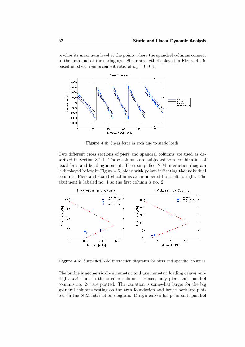
62 Static and Linear Dynamic Analysis
reaches its maximum level at the points where the spandrel columns connectto the arch and at the springings. Shear strength displayed in Figure 4.4 isbased on shear reinforcement ratio of ρw = 0.011.
Figure 4.4: Shear force in arch due to static loads
Two different cross sections of piers and spandrel columns are used as de-scribed in Section 3.1.1. These columns are subjected to a combination ofaxial force and bending moment. Their simplified N-M interaction diagramis displayed below in Figure 4.5, along with points indicating the individualcolumns. Piers and spandrel columns are numbered from left to right. Theabutment is labeled no. 1 so the first column is no. 2.
Figure 4.5: Simplified N-M interaction diagrams for piers and spandrel columns
The bridge is geometrically symmetric and unsymmetric loading causes onlyslight variations in the smaller columns. Hence, only piers and spandrelcolumns no. 2-5 are plotted. The variation is somewhat larger for the bigspandrel columns resting on the arch foundation and hence both are plot-ted on the N-M interaction diagram. Design curves for piers and spandrel

4.2 Original Bridge 63
columns are based on reinforcement ratio of ρl = 0.015 for the small andρl = 0.006 for the big spandrel columns resting on the arch foundation.
Shear forces in the piers and spandrel columns are shown in Figure 4.6 belowalong with a calculated shear strength based on a shear reinforcement ratioof ρw = 0.008 for the smaller columns and ρw = 0.002 for the spandrelcolumns resting on the arch foundation.
Figure 4.6: Shear force in piers and spandrel columns due to static loads. Shearstrength shown with dashed line
Piers closest to abutments are most heavily loaded in shear whereas thespandrel columns resting on the arch foundation carry the smallest portionof the shear force in the design load combination ULS-Temp.
Section forces in the bridge deck were also considered. Bending moment andshear diagrams in the bridge deck are shown in Figures 4.7 and 4.8 belowalong with the calculated moment and shear capacity.
Figure 4.7: Bending moment in bridge deck due to static loads

64 Static and Linear Dynamic Analysis
Figure 4.8: Shear force in bridge deck due to static loads
Moment and shear capacity are based on reinforcement ratios of ρl = 0.013and ρw = 0.006 respectively.
4.2.2 Response to Seismic Loads
In this section the response of the original bridge to seismic loads obtainedfrom Eurocode 8 representing the South Iceland Seismic Zone is illustrated.Section forces are shown and compared to relevant static results from Section4.2.1.
Three different combinations of components of seismic action were consid-ered, Quake-X, Quake-Y and Quake-Z. Each combination includes differentportions of the three components of seismic action as defined in Section3.2.5.
Each seismic combination yields two values at each point since the seismicload works in both directions. Minimum values of seismic combinations areindicated with an asterix in the legends of the figures below. For the sake ofclarity only the most severe combinations are shown in the following figures.
The axial force and bending moment of the arch rib due to the seismic loadare shown in Figure 4.9 along with main results from the static analysis. Itcan be seen that the response spectrum analysis yields larger axial forces andbending moments in the arch. The combination with the vertical seismiccomponent dominating (Quake-Z ) is most severe for the axial force whereasthe combination with longitudinal seismic component as the dominating one(Quake-X ) yields the largest bending moment. Worth noticing is also thelower axial forces obtained. Smaller values for the axial forces is not neces-sarily better because of the nonlinear interaction between bending momentand axial force. Lower axial force can mean a reduced moment capacity.
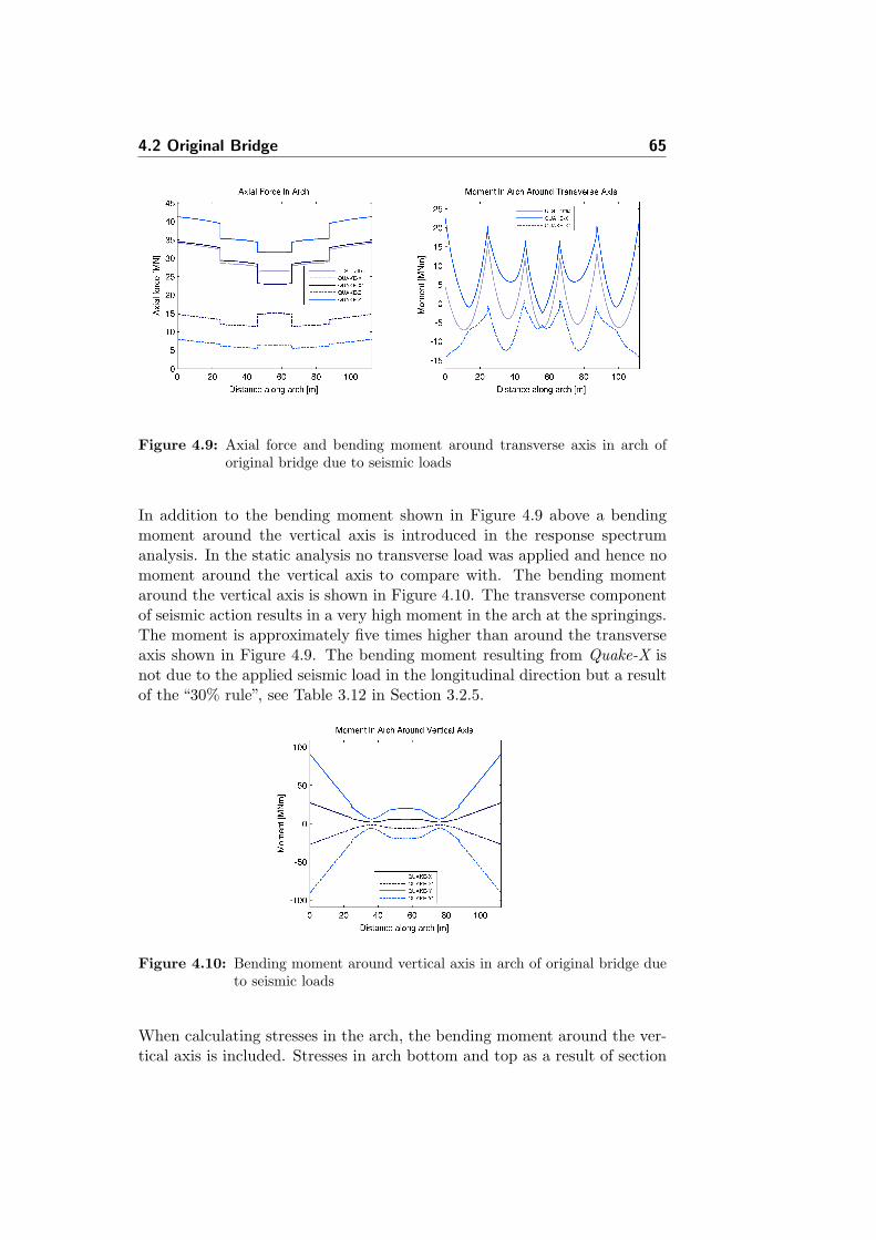
4.2 Original Bridge 65
Figure 4.9: Axial force and bending moment around transverse axis in arch oforiginal bridge due to seismic loads
In addition to the bending moment shown in Figure 4.9 above a bendingmoment around the vertical axis is introduced in the response spectrumanalysis. In the static analysis no transverse load was applied and hence nomoment around the vertical axis to compare with. The bending momentaround the vertical axis is shown in Figure 4.10. The transverse componentof seismic action results in a very high moment in the arch at the springings.The moment is approximately five times higher than around the transverseaxis shown in Figure 4.9. The bending moment resulting from Quake-X isnot due to the applied seismic load in the longitudinal direction but a resultof the “30% rule”, see Table 3.12 in Section 3.2.5.
Figure 4.10: Bending moment around vertical axis in arch of original bridge dueto seismic loads
When calculating stresses in the arch, the bending moment around the ver-tical axis is included. Stresses in arch bottom and top as a result of section
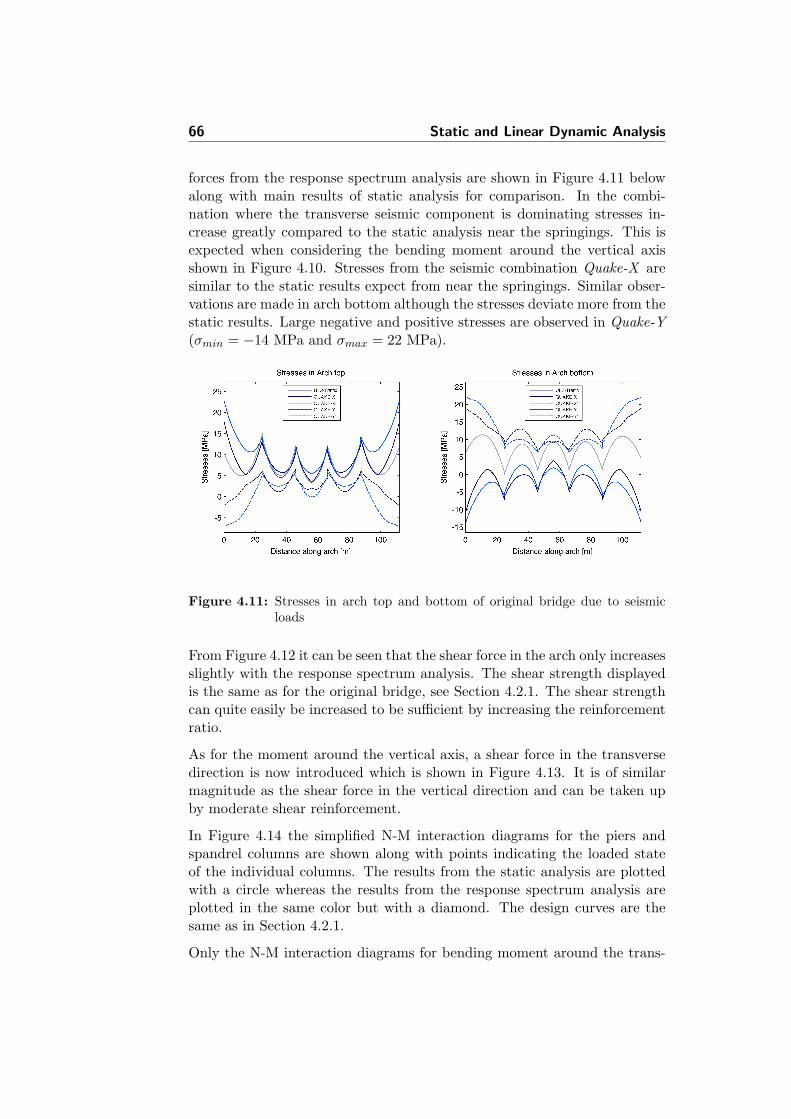
66 Static and Linear Dynamic Analysis
forces from the response spectrum analysis are shown in Figure 4.11 belowalong with main results of static analysis for comparison. In the combi-nation where the transverse seismic component is dominating stresses in-crease greatly compared to the static analysis near the springings. This isexpected when considering the bending moment around the vertical axisshown in Figure 4.10. Stresses from the seismic combination Quake-X aresimilar to the static results expect from near the springings. Similar obser-vations are made in arch bottom although the stresses deviate more from thestatic results. Large negative and positive stresses are observed in Quake-Y(σmin = −14 MPa and σmax = 22 MPa).
Figure 4.11: Stresses in arch top and bottom of original bridge due to seismicloads
From Figure 4.12 it can be seen that the shear force in the arch only increasesslightly with the response spectrum analysis. The shear strength displayedis the same as for the original bridge, see Section 4.2.1. The shear strengthcan quite easily be increased to be sufficient by increasing the reinforcementratio.
As for the moment around the vertical axis, a shear force in the transversedirection is now introduced which is shown in Figure 4.13. It is of similarmagnitude as the shear force in the vertical direction and can be taken upby moderate shear reinforcement.
In Figure 4.14 the simplified N-M interaction diagrams for the piers andspandrel columns are shown along with points indicating the loaded stateof the individual columns. The results from the static analysis are plottedwith a circle whereas the results from the response spectrum analysis areplotted in the same color but with a diamond. The design curves are thesame as in Section 4.2.1.
Only the N-M interaction diagrams for bending moment around the trans-
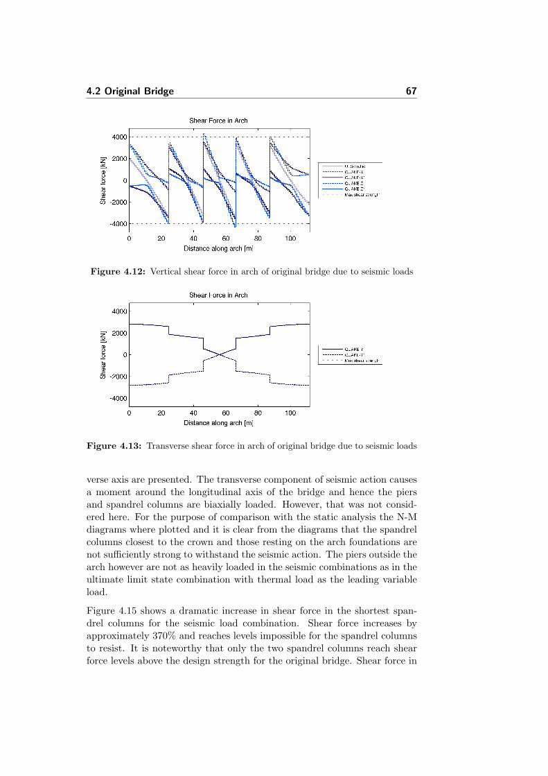
4.2 Original Bridge 67
Figure 4.12: Vertical shear force in arch of original bridge due to seismic loads
Figure 4.13: Transverse shear force in arch of original bridge due to seismic loads
verse axis are presented. The transverse component of seismic action causesa moment around the longitudinal axis of the bridge and hence the piersand spandrel columns are biaxially loaded. However, that was not consid-ered here. For the purpose of comparison with the static analysis the N-Mdiagrams where plotted and it is clear from the diagrams that the spandrelcolumns closest to the crown and those resting on the arch foundations arenot sufficiently strong to withstand the seismic action. The piers outside thearch however are not as heavily loaded in the seismic combinations as in theultimate limit state combination with thermal load as the leading variableload.
Figure 4.15 shows a dramatic increase in shear force in the shortest span-drel columns for the seismic load combination. Shear force increases byapproximately 370% and reaches levels impossible for the spandrel columnsto resist. It is noteworthy that only the two spandrel columns reach shearforce levels above the design strength for the original bridge. Shear force in

68 Static and Linear Dynamic Analysis
Figure 4.14: Simplified N-M interaction diagrams for piers and spandrel columnsof original bridge. Points indicate static and seismic loaded state ofcolumns
the transverse direction is not shown.
Figure 4.15: Shear force in piers and spandrel columns of original bridge due toseismic loads. Shear strength shown with dashed line
Bending moment and shear diagrams in the bridge deck are shown in Figures4.16 and 4.17 below along with the calculated moment and shear capacityand main results from static analysis. Bending moment increases substan-tially in the seismic load combination compared to the results of the staticanalysis. This applies to the section of the bridge deck above the arch only,the approach spans are not heavily influenced by the seismic load combina-tions. Shear forces in the bridge deck do not increase in an seismic event ascan be seen in Figure 4.17. Here, as with the arch, only section forces in theplane of the bridge are shown for reasons of comparison.

4.3 Base Isolated Bridge 69
Figure 4.16: Moment in bridge deck of original bridge due to seismic loads
Figure 4.17: Shear in bridge deck of original bridge due to seismic loads
4.3 Base Isolated Bridge
A response spectrum analysis was performed on the base isolated bridge withthe isolation system described in Section 3.1.3. As with the original bridgethe response spectrum analysis was performed by applying the load definedin Section 3.2.4 in all three directions and combined with load combina-tions as described in Section 3.2.5. In addition to this a response spectrumanalysis was performed on a model without the arch and the columns fixedat their bases for the longitudinal direction only. The purpose of whichwas to make a better comparison of response spectrum analysis and the di-rect displacement-based hand calculations and to adjust the computationalmodel.
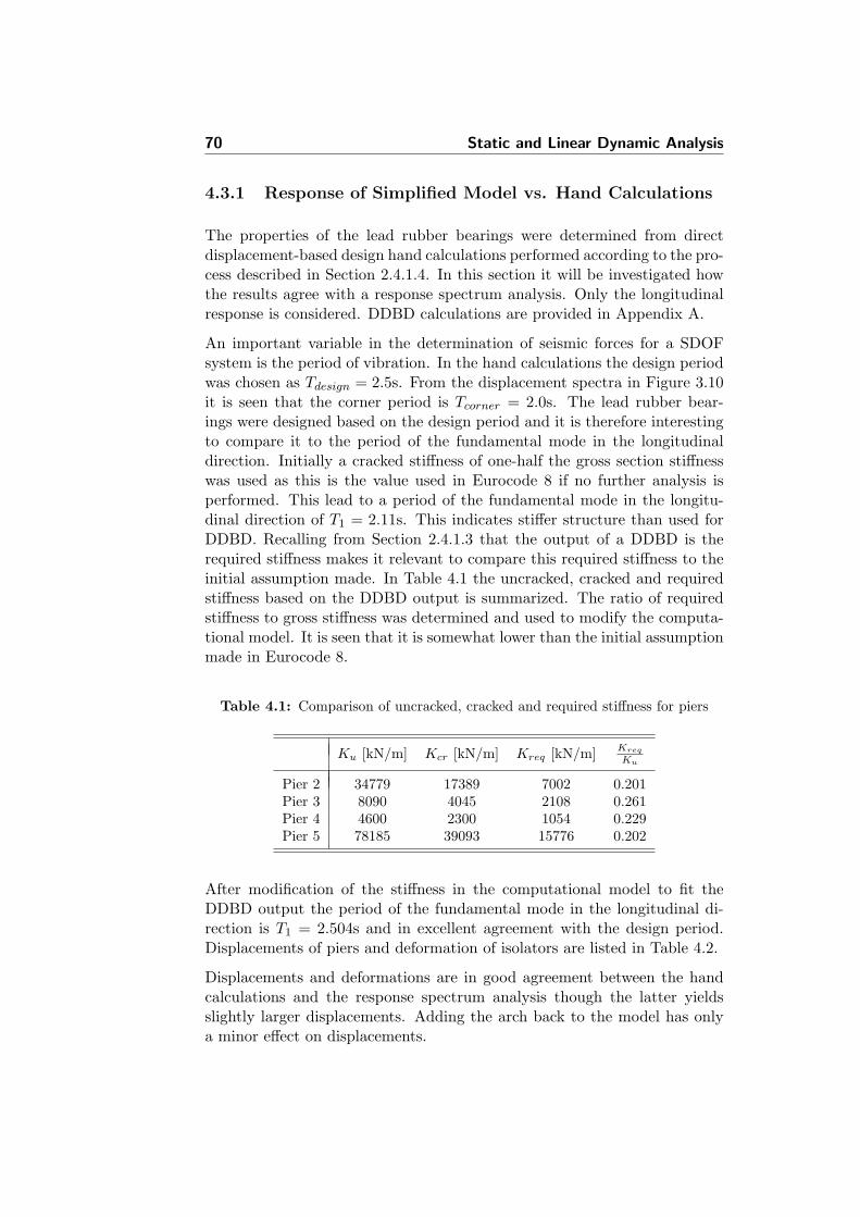
70 Static and Linear Dynamic Analysis
4.3.1 Response of Simplified Model vs. Hand Calculations
The properties of the lead rubber bearings were determined from directdisplacement-based design hand calculations performed according to the pro-cess described in Section 2.4.1.4. In this section it will be investigated howthe results agree with a response spectrum analysis. Only the longitudinalresponse is considered. DDBD calculations are provided in Appendix A.
An important variable in the determination of seismic forces for a SDOFsystem is the period of vibration. In the hand calculations the design periodwas chosen as Tdesign = 2.5s. From the displacement spectra in Figure 3.10it is seen that the corner period is Tcorner = 2.0s. The lead rubber bear-ings were designed based on the design period and it is therefore interestingto compare it to the period of the fundamental mode in the longitudinaldirection. Initially a cracked stiffness of one-half the gross section stiffnesswas used as this is the value used in Eurocode 8 if no further analysis isperformed. This lead to a period of the fundamental mode in the longitu-dinal direction of T1 = 2.11s. This indicates stiffer structure than used forDDBD. Recalling from Section 2.4.1.3 that the output of a DDBD is therequired stiffness makes it relevant to compare this required stiffness to theinitial assumption made. In Table 4.1 the uncracked, cracked and requiredstiffness based on the DDBD output is summarized. The ratio of requiredstiffness to gross stiffness was determined and used to modify the computa-tional model. It is seen that it is somewhat lower than the initial assumptionmade in Eurocode 8.
Table 4.1: Comparison of uncracked, cracked and required stiffness for piers
Ku [kN/m] Kcr [kN/m] Kreq [kN/m] Kreq
Ku
Pier 2 34779 17389 7002 0.201Pier 3 8090 4045 2108 0.261Pier 4 4600 2300 1054 0.229Pier 5 78185 39093 15776 0.202
After modification of the stiffness in the computational model to fit theDDBD output the period of the fundamental mode in the longitudinal di-rection is T1 = 2.504s and in excellent agreement with the design period.Displacements of piers and deformation of isolators are listed in Table 4.2.
Displacements and deformations are in good agreement between the handcalculations and the response spectrum analysis though the latter yieldsslightly larger displacements. Adding the arch back to the model has onlya minor effect on displacements.
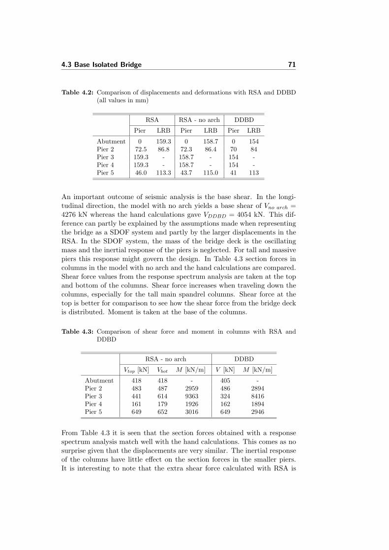
4.3 Base Isolated Bridge 71
Table 4.2: Comparison of displacements and deformations with RSA and DDBD(all values in mm)
RSA RSA - no arch DDBD
Pier LRB Pier LRB Pier LRB
Abutment 0 159.3 0 158.7 0 154Pier 2 72.5 86.8 72.3 86.4 70 84Pier 3 159.3 - 158.7 - 154 -Pier 4 159.3 - 158.7 - 154 -Pier 5 46.0 113.3 43.7 115.0 41 113
An important outcome of seismic analysis is the base shear. In the longi-tudinal direction, the model with no arch yields a base shear of Vno arch =4276 kN whereas the hand calculations gave VDDBD = 4054 kN. This dif-ference can partly be explained by the assumptions made when representingthe bridge as a SDOF system and partly by the larger displacements in theRSA. In the SDOF system, the mass of the bridge deck is the oscillatingmass and the inertial response of the piers is neglected. For tall and massivepiers this response might govern the design. In Table 4.3 section forces incolumns in the model with no arch and the hand calculations are compared.Shear force values from the response spectrum analysis are taken at the topand bottom of the columns. Shear force increases when traveling down thecolumns, especially for the tall main spandrel columns. Shear force at thetop is better for comparison to see how the shear force from the bridge deckis distributed. Moment is taken at the base of the columns.
Table 4.3: Comparison of shear force and moment in columns with RSA andDDBD
RSA - no arch DDBD
Vtop [kN] Vbot M [kN/m] V [kN] M [kN/m]
Abutment 418 418 - 405 -Pier 2 483 487 2959 486 2894Pier 3 441 614 9363 324 8416Pier 4 161 179 1926 162 1894Pier 5 649 652 3016 649 2946
From Table 4.3 it is seen that the section forces obtained with a responsespectrum analysis match well with the hand calculations. This comes as nosurprise given that the displacements are very similar. The inertial responseof the columns have little effect on the section forces in the smaller piers.It is interesting to note that the extra shear force calculated with RSA is
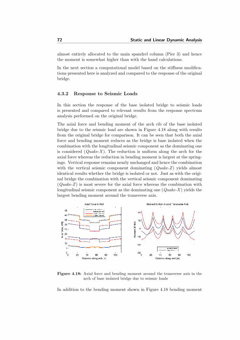
72 Static and Linear Dynamic Analysis
almost entirely allocated to the main spandrel column (Pier 3) and hencethe moment is somewhat higher than with the hand calculations.
In the next section a computational model based on the stiffness modifica-tions presented here is analyzed and compared to the response of the originalbridge.
4.3.2 Response to Seismic Loads
In this section the response of the base isolated bridge to seismic loadsis presented and compared to relevant results from the response spectrumanalysis performed on the original bridge.
The axial force and bending moment of the arch rib of the base isolatedbridge due to the seismic load are shown in Figure 4.18 along with resultsfrom the original bridge for comparison. It can be seen that both the axialforce and bending moment reduces as the bridge is base isolated when thecombination with the longitudinal seismic component as the dominating oneis considered (Quake-X ). The reduction is uniform along the arch for theaxial force whereas the reduction in bending moment is largest at the spring-ings. Vertical response remains nearly unchanged and hence the combinationwith the vertical seismic component dominating (Quake-Z ) yields almostidentical results whether the bridge is isolated or not. Just as with the origi-nal bridge the combination with the vertical seismic component dominating(Quake-Z ) is most severe for the axial force whereas the combination withlongitudinal seismic component as the dominating one (Quake-X ) yields thelargest bending moment around the transverse axis.
Figure 4.18: Axial force and bending moment around the transverse axis in thearch of base isolated bridge due to seismic loads
In addition to the bending moment shown in Figure 4.18 bending moment
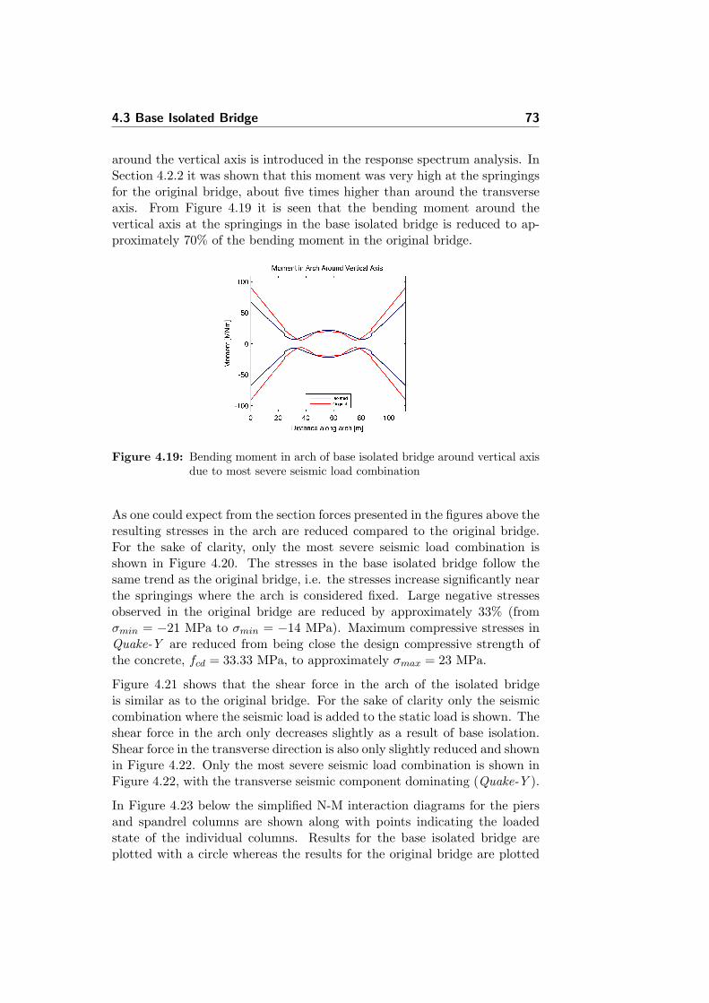
4.3 Base Isolated Bridge 73
around the vertical axis is introduced in the response spectrum analysis. InSection 4.2.2 it was shown that this moment was very high at the springingsfor the original bridge, about five times higher than around the transverseaxis. From Figure 4.19 it is seen that the bending moment around thevertical axis at the springings in the base isolated bridge is reduced to ap-proximately 70% of the bending moment in the original bridge.
Figure 4.19: Bending moment in arch of base isolated bridge around vertical axisdue to most severe seismic load combination
As one could expect from the section forces presented in the figures above theresulting stresses in the arch are reduced compared to the original bridge.For the sake of clarity, only the most severe seismic load combination isshown in Figure 4.20. The stresses in the base isolated bridge follow thesame trend as the original bridge, i.e. the stresses increase significantly nearthe springings where the arch is considered fixed. Large negative stressesobserved in the original bridge are reduced by approximately 33% (fromσmin = −21 MPa to σmin = −14 MPa). Maximum compressive stresses inQuake-Y are reduced from being close the design compressive strength ofthe concrete, fcd = 33.33 MPa, to approximately σmax = 23 MPa.
Figure 4.21 shows that the shear force in the arch of the isolated bridgeis similar as to the original bridge. For the sake of clarity only the seismiccombination where the seismic load is added to the static load is shown. Theshear force in the arch only decreases slightly as a result of base isolation.Shear force in the transverse direction is also only slightly reduced and shownin Figure 4.22. Only the most severe seismic load combination is shown inFigure 4.22, with the transverse seismic component dominating (Quake-Y ).
In Figure 4.23 below the simplified N-M interaction diagrams for the piersand spandrel columns are shown along with points indicating the loadedstate of the individual columns. Results for the base isolated bridge areplotted with a circle whereas the results for the original bridge are plotted
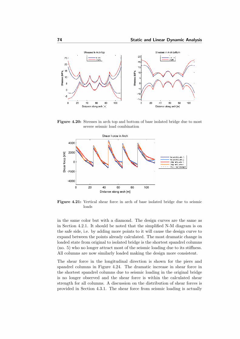
74 Static and Linear Dynamic Analysis
Figure 4.20: Stresses in arch top and bottom of base isolated bridge due to mostsevere seismic load combination
Figure 4.21: Vertical shear force in arch of base isolated bridge due to seismicloads
in the same color but with a diamond. The design curves are the same asin Section 4.2.1. It should be noted that the simplified N-M diagram is onthe safe side, i.e. by adding more points to it will cause the design curve toexpand between the points already calculated. The most dramatic change inloaded state from original to isolated bridge is the shortest spandrel columns(no. 5) who no longer attract most of the seismic loading due to its stiffness.All columns are now similarly loaded making the design more consistent.
The shear force in the longitudinal direction is shown for the piers andspandrel columns in Figure 4.24. The dramatic increase in shear force inthe shortest spandrel columns due to seismic loading in the original bridgeis no longer observed and the shear force is within the calculated shearstrength for all columns. A discussion on the distribution of shear forces isprovided in Section 4.3.1. The shear force from seismic loading is actually

4.3 Base Isolated Bridge 75
Figure 4.22: Transverse shear force in arch of base isolated bridge due to seismicloads
Figure 4.23: Simplified N-M interaction diagrams for piers and spandrel columnsof base isolated bridge. Points indicate static and seismic loadedstate of columns
lower than that resulting from the load combination with temperature loadas the leading live load.
Bending moment and shear diagrams for the bridge deck are shown in Fig-ures 4.25 and 4.26. Results for the original bridge are not included in figuresbelow but they can be seen in Figures 4.16 and 4.17. It is seen that thebending moment resulting from seismic load combinations is reduced com-pared to the original bridge but does still exceed the calculated momentcapacity. Finally it is worth noticing that for the isolated bridge it is theseismic load combination with the vertical seismic component as the dom-inating one (Quake-Z) that is the most severe and not the one with thelongitudinal seismic component (Quake-X ) as was the case for the originalbridge. Shear forces in the bridge deck of the base isolated bridge do notincrease dramatically in a seismic event.
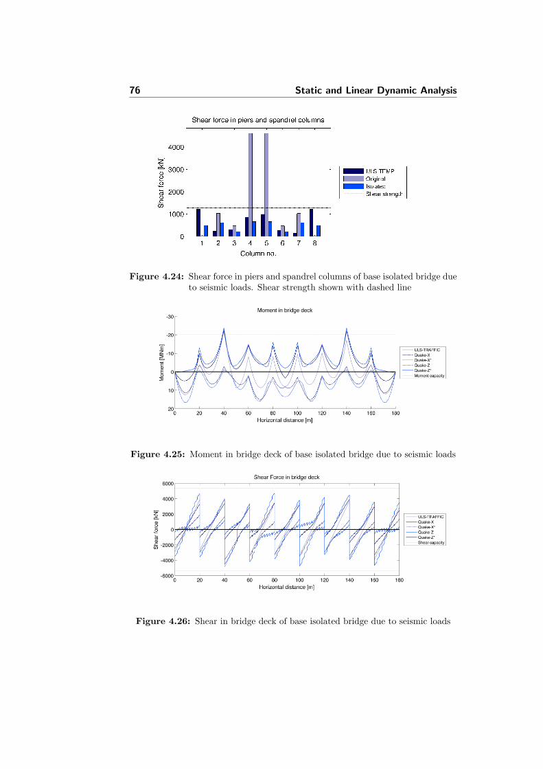
76 Static and Linear Dynamic Analysis
Figure 4.24: Shear force in piers and spandrel columns of base isolated bridge dueto seismic loads. Shear strength shown with dashed line
Figure 4.25: Moment in bridge deck of base isolated bridge due to seismic loads
Figure 4.26: Shear in bridge deck of base isolated bridge due to seismic loads

4.4 Thoughts on Redesign 77
4.4 Thoughts on Redesign
In this section some thoughts on possible redesign of the bridge elements arepresented. Based on the results presented above it is clear that seismic isola-tion alone is not sufficient to provide satisfactory safety against earthquakes.Each structural element is treated separately.
1. Bridge Deck
2. Piers and Spandrel Columns
3. The Arch
1. The bridge deck is made of non-prestressed reinforced concrete. From allthe analysis performed it is clear that the mass of the bridge deck is one of themost important factors. It is obvious that reducing the mass of the bridgedeck would reduce the base shear since the base shear is directly proportionalto the mass of the bridge deck through Equations 2.28 and 2.29. Reducingthe mass of the bridge deck by considering prestressing of the bridge deckor perhaps a composite bridge deck made of steel and concrete is the firstthing to be considered when redesigning the bridge. Reducing the mass ofthe bridge deck will have an advantageous effect on the substructure.
2. The response of piers and spandrel columns is improved when the bridgeis seismically isolated and are very close to being within the simplified designcurves presented in Figure 4.23. It should however be kept in mind that inthose figures only the bending moment around the transverse axis is consid-ered despite the fact that the columns are biaxially loaded. Once redesignof the bridge deck has taken place it is likely that the original cross sectionof piers and spandrel columns can provide sufficient strength. Despite thatthe cross section type should be altered since a hollow square section is notconsidered very suitable for seismic loading [Priestley et al. (2007)]. A circu-lar solid column would be more desirable since it makes it easier to provideadequate restraint against buckling of longitudinal reinforcement and alsobecause a circular column exhibits the same properties in all directions.
3. Response of the arch strongly indicates that redesign is needed. Anincrease in the cross section of the arch towards its fixity in the foundationsshould be introduced. That will severely increase the moment of inertia andthus decrease the stresses at the springings. The stresses and moment inthe arch are not reduced as much as section forces in columns when thebridge is seismically isolated. This is not surprising since it is the seismiccombination with the vertical component as the dominating one that is theworst case scenario for the arch and the bridge is not isolated in the verticaldirection.

Chapter 5
Time History Analysis
5.1 Introduction
To study the response of the base isolation system further, the computationalmodel described in Section 4.1 was analyzed with time history analysis usingartificial accelerograms. Only the longitudinal response is studied in thischapter.
The development of the model for time history analysis was a somewhat dif-ficult task. In general purpose FE-programs like SAP2000 there are usuallyseveral integration schemes available and various variables can be adjusted toinfluence the result. Creating a model and setting the parameters such thatthe outcome of the analysis was in agreement with expected outcome wasa tedious task. The process is very time consuming since the time historyanalysis using direct integration can be very expensive on computationaltime.
In the very beginning the Hilbert-Hughes-Taylor method was used since itis the one recommended in the documentation to SAP2000. The method isan improved version of the Newmark method. However it yielded unstableresults and as a consequence other options were reviewed. After numeroustest runs on a simple model the decision was made to use the Newmarkaverage acceleration algorithm which is described in Section 2.5.2.
Comparison of nonlinear time history analysis to response spectrum anal-ysis is not easily interpreted. Several variables affect the result and makesdirect comparison difficult. A major uncertainty regarding the nonlinear

80 Time History Analysis
response of the isolated bridge is the damping provided by the isolators.In the response spectrum analysis the hysteretic damping is described withequivalent viscous damping and the response spectrum is split into two partsto capture the damping effect of the bearings. In a nonlinear analysis thedamping is calculated directly from the hysteretic response. Hence, it is notreasonable to draw any conclusion about the outcome of the nonlinear timehistory analysis by comparison to response spectrum analysis results.
A more transparent way of viewing the results of time history analysis isneglecting the nonlinear behavior and perform a linear time history analy-sis using the equivalent properties of the isolators as described in Section3.1.3. Plotting the displacement spectra of the artificial time histories andcomparing them to the output maximum displacement obtained with lineartime history analysis can give an indication as to whether or not the timehistory results are yielding expected results. Below in Table 5.1 the maxi-mum horizontal displacement of the bridge deck is listed for each of the tenartificial time histories as well as from the response spectrum analysis. InFigure 5.1 the displacement spectra for the time histories are plotted.
Results from the time history analysis are in good agreement with responsespectrum analysis and the displacement spectra. Now nonlinear propertiescan be included in the model and the response studied further.
Figure 5.1: Displacement spectra for artificial time histories and Eurocode 8. Dis-placements in m
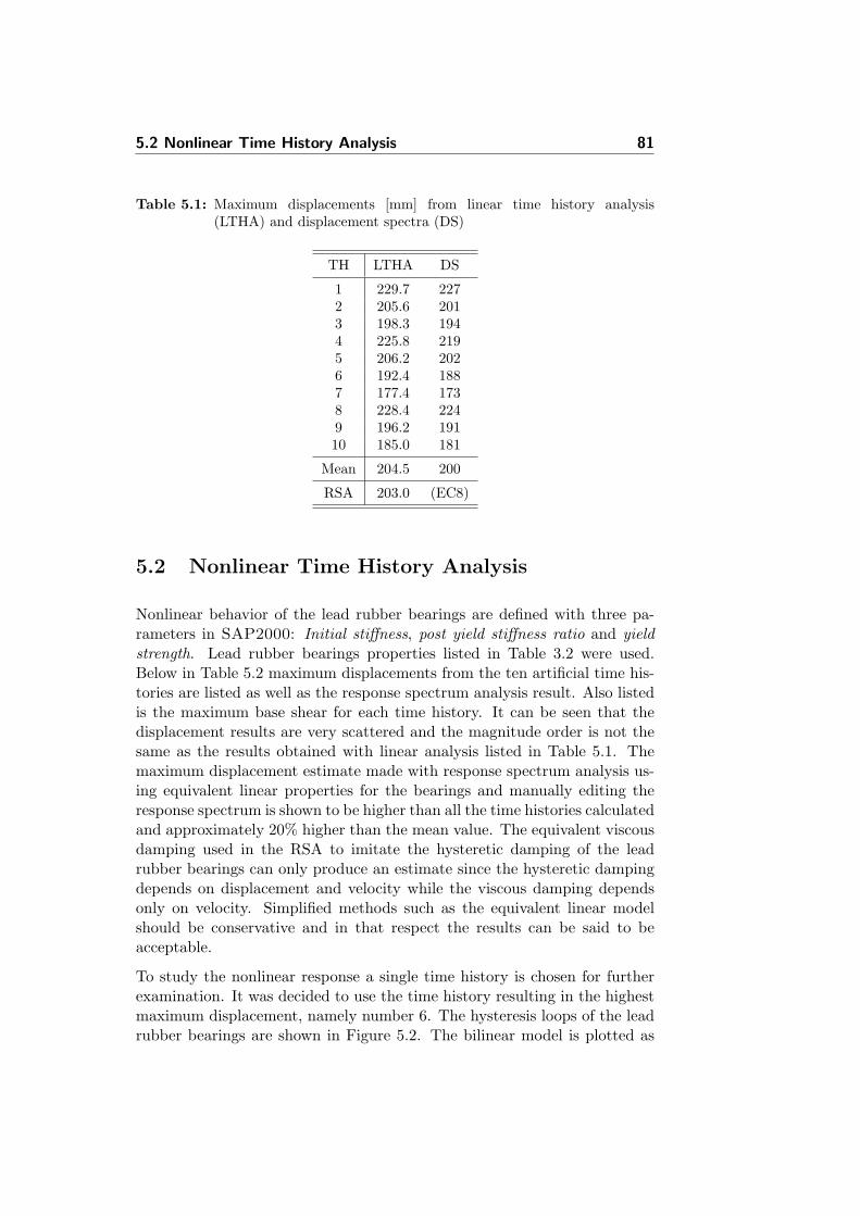
5.2 Nonlinear Time History Analysis 81
Table 5.1: Maximum displacements [mm] from linear time history analysis(LTHA) and displacement spectra (DS)
TH LTHA DS
1 229.7 2272 205.6 2013 198.3 1944 225.8 2195 206.2 2026 192.4 1887 177.4 1738 228.4 2249 196.2 19110 185.0 181
Mean 204.5 200
RSA 203.0 (EC8)
5.2 Nonlinear Time History Analysis
Nonlinear behavior of the lead rubber bearings are defined with three pa-rameters in SAP2000: Initial stiffness, post yield stiffness ratio and yieldstrength. Lead rubber bearings properties listed in Table 3.2 were used.Below in Table 5.2 maximum displacements from the ten artificial time his-tories are listed as well as the response spectrum analysis result. Also listedis the maximum base shear for each time history. It can be seen that thedisplacement results are very scattered and the magnitude order is not thesame as the results obtained with linear analysis listed in Table 5.1. Themaximum displacement estimate made with response spectrum analysis us-ing equivalent linear properties for the bearings and manually editing theresponse spectrum is shown to be higher than all the time histories calculatedand approximately 20% higher than the mean value. The equivalent viscousdamping used in the RSA to imitate the hysteretic damping of the leadrubber bearings can only produce an estimate since the hysteretic dampingdepends on displacement and velocity while the viscous damping dependsonly on velocity. Simplified methods such as the equivalent linear modelshould be conservative and in that respect the results can be said to beacceptable.
To study the nonlinear response a single time history is chosen for furtherexamination. It was decided to use the time history resulting in the highestmaximum displacement, namely number 6. The hysteresis loops of the leadrubber bearings are shown in Figure 5.2. The bilinear model is plotted as
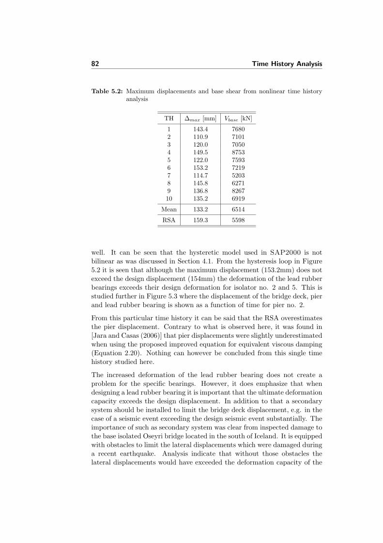
82 Time History Analysis
Table 5.2: Maximum displacements and base shear from nonlinear time historyanalysis
TH ∆max [mm] Vbase [kN]
1 143.4 76802 110.9 71013 120.0 70504 149.5 87535 122.0 75936 153.2 72197 114.7 52038 145.8 62719 136.8 826710 135.2 6919
Mean 133.2 6514
RSA 159.3 5598
well. It can be seen that the hysteretic model used in SAP2000 is notbilinear as was discussed in Section 4.1. From the hysteresis loop in Figure5.2 it is seen that although the maximum displacement (153.2mm) does notexceed the design displacement (154mm) the deformation of the lead rubberbearings exceeds their design deformation for isolator no. 2 and 5. This isstudied further in Figure 5.3 where the displacement of the bridge deck, pierand lead rubber bearing is shown as a function of time for pier no. 2.
From this particular time history it can be said that the RSA overestimatesthe pier displacement. Contrary to what is observed here, it was found in[Jara and Casas (2006)] that pier displacements were slightly underestimatedwhen using the proposed improved equation for equivalent viscous damping(Equation 2.20). Nothing can however be concluded from this single timehistory studied here.
The increased deformation of the lead rubber bearing does not create aproblem for the specific bearings. However, it does emphasize that whendesigning a lead rubber bearing it is important that the ultimate deformationcapacity exceeds the design displacement. In addition to that a secondarysystem should be installed to limit the bridge deck displacement, e.g. in thecase of a seismic event exceeding the design seismic event substantially. Theimportance of such as secondary system was clear from inspected damage tothe base isolated Oseyri bridge located in the south of Iceland. It is equippedwith obstacles to limit the lateral displacements which were damaged duringa recent earthquake. Analysis indicate that without those obstacles thelateral displacements would have exceeded the deformation capacity of the
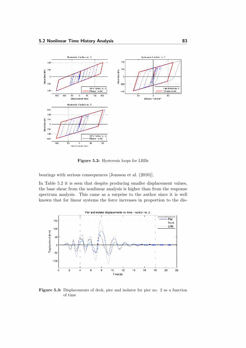
5.2 Nonlinear Time History Analysis 83
Figure 5.2: Hysteresis loops for LRBs
bearings with serious consequences [Jonsson et al. (2010)].
In Table 5.2 it is seen that despite producing smaller displacement values,the base shear from the nonlinear analysis is higher than from the responsespectrum analysis. This came as a surprise to the author since it is wellknown that for linear systems the force increases in proportion to the dis-
Figure 5.3: Displacements of deck, pier and isolator for pier no. 2 as a functionof time
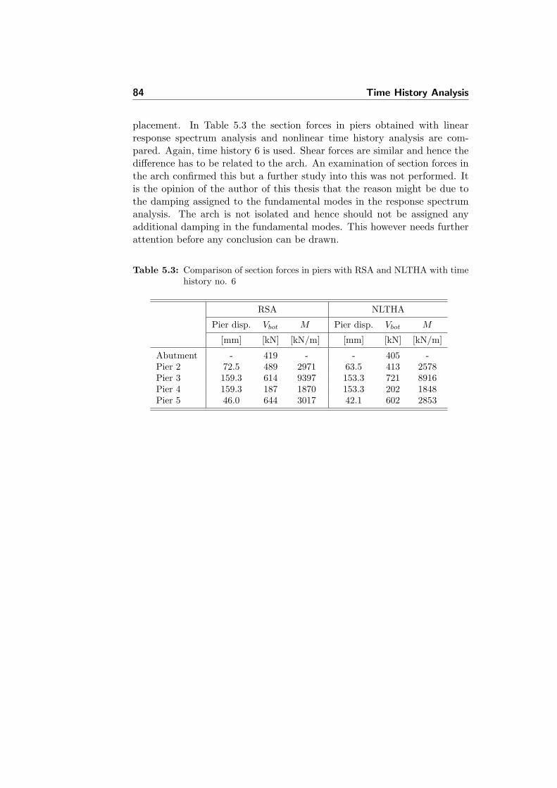
84 Time History Analysis
placement. In Table 5.3 the section forces in piers obtained with linearresponse spectrum analysis and nonlinear time history analysis are com-pared. Again, time history 6 is used. Shear forces are similar and hence thedifference has to be related to the arch. An examination of section forces inthe arch confirmed this but a further study into this was not performed. Itis the opinion of the author of this thesis that the reason might be due tothe damping assigned to the fundamental modes in the response spectrumanalysis. The arch is not isolated and hence should not be assigned anyadditional damping in the fundamental modes. This however needs furtherattention before any conclusion can be drawn.
Table 5.3: Comparison of section forces in piers with RSA and NLTHA with timehistory no. 6
RSA NLTHA
Pier disp. Vbot M Pier disp. Vbot M
[mm] [kN] [kN/m] [mm] [kN] [kN/m]
Abutment - 419 - - 405 -Pier 2 72.5 489 2971 63.5 413 2578Pier 3 159.3 614 9397 153.3 721 8916Pier 4 159.3 187 1870 153.3 202 1848Pier 5 46.0 644 3017 42.1 602 2853

Chapter 6
Summary and Conclusions
In this thesis the response of an idealized concrete arch bridge to seismicloading occurring in the South Iceland Seismic Zone is presented. Originallythe bridge was not designed for seismic loading and it is shown that modifi-cation to the design concept is required if it were to be erected in the Southof Iceland. The design earthquake load was obtained from Eurocode 8 andthe Icelandic National Annex. Characteristic peak ground acceleration inthe South Iceland Seismic Zone is 0.4g for a design earthquake with 475 yearreturn period.
To improve the response seismic isolation was considered. A direct displace-ment-based design procedure for bridges supported on isolation bearingswith bilinear characteristics is presented. The procedure is applied to thelongitudinal response but is equally well suited for transverse response. Theapproach is compared to the traditional force-based design approach andshown to be more transparent and enables the designer to control the to-tal structural response during the design process in a simple manner. Anisolation system using lead rubber bearings is designed with simple handcalculations idealizing the bridge as a single degree of freedom system. Itsresponse is estimated directly from the elastic displacement response spectraby use of an effective period and equivalent viscous damping.
A response spectrum analysis is performed on the isolated bridge and theresponse is compared to the response of the original bridge. The isolatedbridge is exactly the same as the original except for the isolation system.Lead rubber bearings are provided on top of half of the piers and span-drel columns and at the abutments. The response is severely improved but

86 Summary and Conclusions
further re-design is considered necessary.
From consideration of the seismicity it can be concluded that the most criti-cal structural elements in the original bridge are the short spandrel columns.They can be effectively protected by designing an appropriate isolation sys-tem. The arch response is only slightly improved by the seismic isolation.However, a moderate increase in the arch cross section towards its fixity inthe foundations would greatly increase safety against seismic loading.
Nonlinear time history analysis was performed using ten artificial time his-tories and the response compared to the linear response spectrum analysis.The well known program Simqke was used to create time histories withresponse spectra similar to the smooth Eurocode 8 design spectrum. Themaximum displacement prediction made with the equivalent linear modelwas shown to remain on the safe side for all time histories. Base shearwas shown to be underestimated with the response spectrum analysis. Acloser examination of a single time history showed that the underestimationwas limited to the response of the arch. This should be studied further todetermine whether the application of a composite spectrum to capture thedamping of the isolators underestimates arch forces. Examination of thesame time history also revealed slightly overestimated pier displacementswith the linear equivalent methods and hence underestimated isolator de-formation.

Bibliography
Bessason, B. and Haflidason, E. (2004). Recorded and numerical strongmotion response of a base-isolated bridge. Earthquake Spectra, 20(2):309–332.
Bommer, J. J. and Acevedo, A. B. (2004). The use of real earthquakeaccelerograms as input to dynamic analysis. Journal of Earthquake Engi-neering, 8(1SPECI):43.
Chopra, A. K. (2007). Dynamics of Structures: Theory and Application toEarthquake Engineering. Pearson Prentice Hall, 3rd edition.
Computers and Structures Inc. (2007). CSI Analysis Reference Manual.Computers and Structures Inc, Berkeley.
Dusseau, R. A. and Wen, R. K. (1989). Seismic responses of deck-type archbridges. Earthquake Engineering & Structural Dynamics, 18(5):701–715.
Iceland Meteorological Office (2010). Weather records - retrieved february15th 2010. http://www.vedur.is/vedur/vedurfar/upplysingar/vedurmet/.
Jangid, R. (2004). Seismic response of isolated bridges. Journal of BridgeEngineering, 9(2):156–166.
Jara, M. and Casas, J. R. (2006). A direct displacement-based method forthe seismic design of bridges on bi-linear isolation devices. EngineeringStructures, 28(6):869–879.
Jensen, B. C., editor (2003). Teknisk Stabi. Ingeniøren Bøger, 18th edition.
Jensen, B. C. (2006). Betonkonstruktioner. Nyt Teknisk Forlag, 3rd edition.
Jonsson, M. H., Bessason, B., and Haflidason, E. (2010). Earthquake re-sponse of a base-isolated bridge subjected to strong near-fault groundmotion. Soil Dynamics and Earthquake Engineering, 30(6):447–455.

88 BIBLIOGRAPHY
Lestuzzi, P. (2002). Simseisme - retrieved march 15th 2010.http://imacwww.epfl.ch/ Team/Lestuzzi/Software/SimSeisme/Sim-Seisme.htm.
Megson, T. (2002). Structural and Stress Analysis. Butterworth-Heinemann.
Naeim, F. and Kelly, J. (1999). Design of Seismic Isolated Structures. Wiley.
Neaz Sheikh, M., Tsang, H., and Lam, N. (2008). Estimation of yield cur-vature for direct displacement-based seismic design of rc columns. InAustralian Earthquake Engineering Conference AEES.
Park, Y. J., Wen, Y. K., and Ang, A. H.-S. (1986). Random vibrationof hysteretic systems under bi-directional ground motions. EarthquakeEngineering & Structural Dynamics, 14(4):543–557.
Priestley, M. (2000). Performance based seismic design. Bulletin of the NewZealand National Society for Earthquake Engineering, 33(3):325–346.
Priestley, M., Calvi, G., and Kowalsky, M. (2007). Displacement-BasedSeismic Design of Structures. IUSS Press, Pavia, Italy.
Priestley, M., Seible, F., and Calvi, G. (1996). Seismic Design and Retrofitof Bridges. John Wiley & Sons, Inc.
Skinner, R. (1993). An Introduction to Seismic Isolation. John Wiley &Sons, Inc.
Wen, Y.-K. (1976). Method for random vibration of hysteretic systems.ASCE J Eng Mech Div, 102(2):249–263.

Appendix A
Direct Displacement-basedHand Calculations


Direct Displacement-based Design of an Isolated Bridge numbers correspond to DDBD flowchart, Figure 2.11
Initial Input Parameters
Bridge deck cross section area: Ad 9.09m2
:=
Length of bridge deck: Ld 180m:=
Density of RC ρ 25kN
m3
:=
=> Mass of bridge deck: Md Ad Ld⋅ ρ⋅ 40905 kN⋅=:=
Deck span: span 20m:=
=> Tributary masses to piers and abutments:
M1
span
2
Ld
Md⋅:= M2span
Ld
Md⋅:= M3 M2:= M4 M2:= M5 M2:=
Depth of concrete pier sections:
hc1 750mm:= hc2 1800mm:=
Height of piers (and abutments):
H1 0m:= H2 5.95m:= H3 26.1m:= H4 11.828m:= H5 4.542m:=
longitudinal reinforcement yield strain: εy 2.5 103−
×:=
Yield strength of reinforcement: fye 435:=
Diameter of rebars dbl 16mm:=
=> Strain penetration depth: Lsp 0.022fye dbl⋅ 0.153m=:=
Determination of design displacement (1)
It is considered acceptable to design for a displacement equal to that corresponding to
the corner period but a longer period is chosen as design period.
Design period: Te 2.5s:=
=> corresponding displacement based on 5% viscous damping from
displacement spectra:
∆T0.05 200mm:=
Reduced displacement found by iteration, see below.
∆e 153mm:=
System equivalent stiffness (4)
Ke
4 π2
⋅ Md⋅
g Te2
⋅
26347kN
m⋅=:=

Yield displacement of each pier (2)
Yield curvature is determined from depth of cross
section and yield strain of reinforcement
Small columns: ϕy.1
2.1 εy⋅
hc1
7 103−
×1
m=:= Big columns: ϕy.2
2.1 εy⋅
hc2
2.917 103−
×1
m=:=
Yield displacement of each pier is then:
∆Py.1 0mm:=
∆Py.2 ϕy.1
H2 Lsp+( )2
3⋅ 87 mm⋅=:=
∆Py.3 ϕy.2
H3 Lsp+( )2
3⋅ 670 mm⋅=:=
∆Py.4 ϕy.1
H4 Lsp+( )2
3⋅ 335 mm⋅=:=
∆Py.5 ϕy.1
H5 Lsp+( )2
3⋅ 51 mm⋅=:=
Note: yield displacement of piers 3 and 4 is much larger than maximum estimated displacement
=> Those piers do not need isolation to remain elastic.
Effective displacement of each isolator
Note: assuming that the force in each isolator at the expected displacement will be X% of the yield
force of each pier. The percentage is different because of different yield displacement of piers
∆DE.1 ∆e 0.8 ∆Py.1⋅− 153 mm⋅=:=
∆DE.2 ∆e 0.8 ∆Py.2⋅− 83 mm⋅=:=
∆DE.3 max ∆e 0.8 ∆Py.3⋅− 0, ( ) 0 mm⋅=:=
∆DE.4 max ∆e 0.8 ∆Py.4⋅− 0, ( ) 0 mm⋅=:=
∆DE.5 ∆e 0.8 ∆Py.5⋅− 112 mm⋅=:=
Assumed equivalent viscous damping ratios for the isolation system (3) Note: initial value is assumed and subsequently the damping is calculated from lead rubber
bearing properties calculated in seperate document.
ξ1 0.20:= ξ2 0.15:= ξ3 0:= ξ4 0:= ξ5 0.16:=
Elastic damping ratio for piers: ξel 0.05:=

Equivalent viscous damping of each pier-isolation system (8)
ξP1
ξ1 ∆DE.1⋅ ξel ∆e ∆DE.1−( )⋅+
∆e
0.2=:=
ξP2
ξ2 ∆DE.2⋅ ξel ∆e ∆DE.2−( )⋅+
∆e
0.105=:=
ξP3
ξ3 ∆DE.3⋅ ξel ∆e ∆DE.3−( )⋅+
∆e
0.05=:=
ξP4
ξ4 ∆DE.4⋅ ξel ∆e ∆DE.4−( )⋅+
∆e
0.05=:=
ξP5
ξ5 ∆DE.5⋅ ξel ∆e ∆DE.5−( )⋅+
∆e
0.13=:=
Shear distribution between piers determine (5)
Division of shear to piers (in %):
P1 10:= P2 12:= P3 8:= P4 4:= P5 16:=
Global equivalent viscous damping (9)
ξsys
2 ξP1 P1⋅ ξP2 P2⋅+ ξP3 P3⋅+ ξP4 P4⋅+ ξP5 P5⋅+( )⋅
1000.119=:=
Damping reduction factor (10)
Rξ0.10
0.05 ξsys+
0.5
0.77=:=
Displacement from reduced displacement spectra (11)
check with design
displacement above!
Iterate if necessary.
∆ξ ∆T0.05 Rξ⋅ 0.154m=:=
Base shear and section forces (12 & 14)
Base shear: Vbase Ke ∆ξ⋅ 4056 kN⋅=:=
Base shear coefficient: kNm kN m⋅:=
Vbase
Md
0.099=
Distribute Vbase to columns and calculate moment:
V1 VbaseP1
100⋅ 406 kN⋅=:=
V2 VbaseP2
100⋅ 487 kN⋅=:= MP2 V2 H2⋅ 2896 kNm⋅=:=
V3 VbaseP3
100⋅ 324 kN⋅=:= MP3 V3 H3⋅ 8468 kNm⋅=:=

V4 VbaseP4
100⋅ 162 kN⋅=:= MP4 V4 H4⋅ 1919 kNm⋅=:=
V5 VbaseP5
100⋅ 649 kN⋅=:= MP5 V5 H5⋅ 2947 kNm⋅=:=
Stiffness of each pier-isolation system (5)
K1
P1 Ke⋅
1002635
kN
m⋅=:= K2
P2 Ke⋅
1003162
kN
m⋅=:= K3
P3 Ke⋅
1002108
kN
m⋅=:=
K4
P4 Ke⋅
1001054
kN
m⋅=:= K5
P5 Ke⋅
1004216
kN
m⋅=:=
Effective stiffness of isolaters and columns. Imposing the design requirement that the
isolater effective force must be equal to 80% of the yielding force of the column (6)
Isolators:
KDE.1 1 0.8∆Py.1
∆DE.1
⋅+
K1⋅ 2635
kN
m⋅=:=
KDE.2 1 0.8∆Py.2
∆DE.2
⋅+
K2⋅ 5795
kN
m⋅=:=
KDE.5 1 0.8∆Py.5
∆DE.5
⋅+
K5⋅ 5766
kN
m⋅=:=
Piers:
KP.2 KDE.2
∆DE.2
0.8 ∆Py.2⋅⋅ 6957
kN
m⋅=:= KP.4 K4 1054
kN
m⋅=:=
KP.3 K3 2108kN
m⋅=:= KP.5 KDE.5
∆DE.5
0.8 ∆Py.5⋅⋅ 15674
kN
m⋅=:=
These values are used to design the lead rubber bearings in a seperate document (7). From
those calculations a equivalent viscous damping value of the isolator is obtained and used
in (3). A few iterations might be necessary.
Required yield moment to achieve required stiffness is calculated with:
Vy2 ∆Py.2 KP.2⋅ 605 kN⋅=:= My2 Vy2 H2⋅ 3598 kNm⋅=:=
Vy3 ∆Py.3 KP.3⋅ 1412 kN⋅=:= My3 Vy3 H3⋅ 36863 kNm⋅=:=
Vy4 ∆Py.4 KP.4⋅ 353 kN⋅=:= My4 Vy4 H4⋅ 4175 kNm⋅=:=
Vy5 ∆Py.5 KP.5⋅ 806 kN⋅=:= My5 Vy5 H5⋅ 3662 kNm⋅=:=


www.byg.dtu.dk
Department of Civil EngineeringTechnical University of DenmarkBrovej Building 118DK-2800 Kgs. LyngbyDenmarkTel: (+45) 45 25 17 00Email: [email protected]


