Page 1
SEISMIC ANALYSIS OF CONCRETE GRAVITY DAMS INCLUDING DAM-
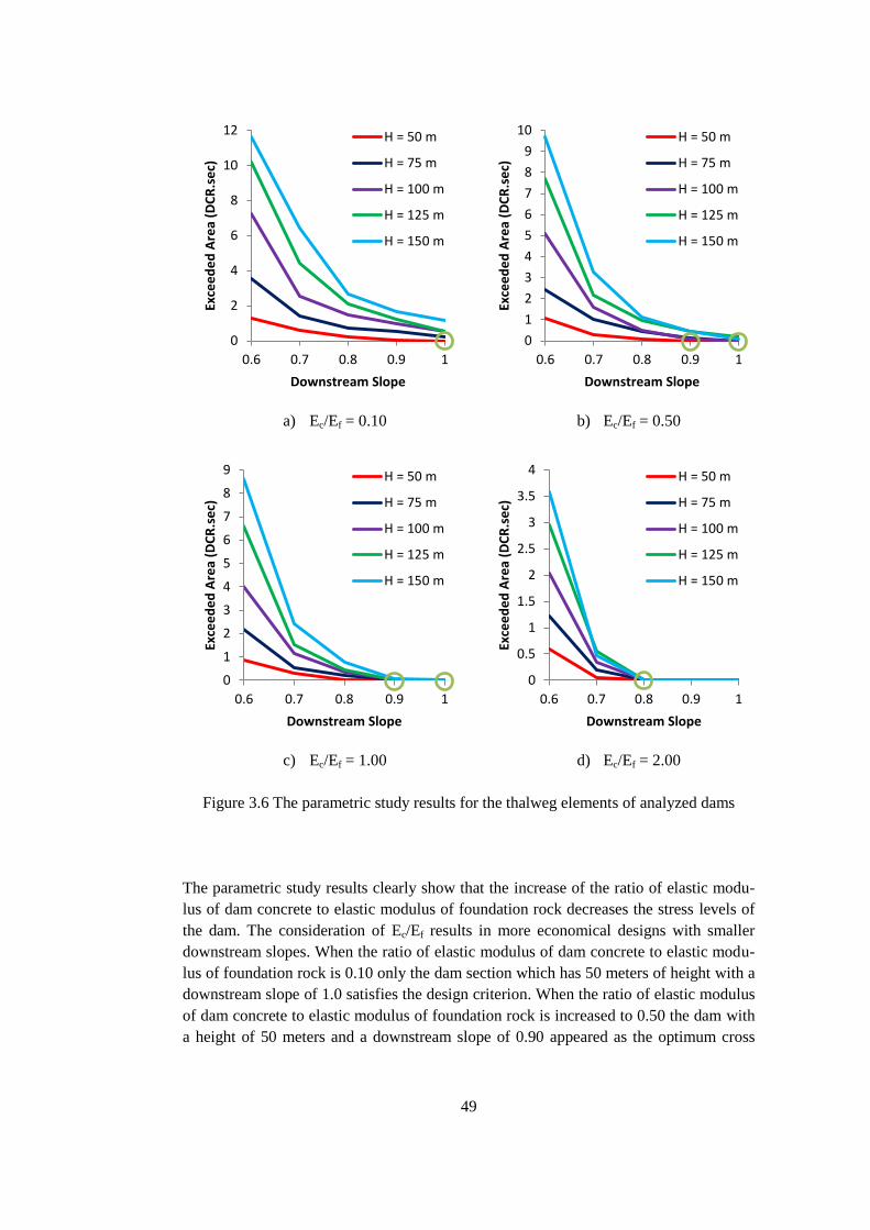
FOUNDATION-RESERVOIR INTERACTION
A THESIS SUBMITTED TO
THE GRADUATE SCHOOL OF NATURAL AND APPLIED SCIENCES
OF
MIDDLE EAST TECHNICAL UNIVERSITY
BY
ALİ RIZA YÜCEL
IN PARTIAL FULFILLMENT OF THE REQUIREMENTS
FOR
THE DEGREE OF MASTER OF SCIENCE
IN
CIVIL ENGINEERING
SEPTEMBER 2013
Page 3
Approval of the thesis:
SEISMIC ANALYSIS OF CONCRETE GRAVITY DAMS INCLUDING DAM-
FOUNDATION-RESERVOIR INTERACTION
submitted by ALİ RIZA YÜCEL in partial fulfillment of the requirements for the de-
gree of Master of Science in Civil Engineering Department, Middle East Technical
University by,
Prof. Dr. Canan Özgen __________________
Dean, Graduate School of Natural and Applied Sciences
Prof. Dr. Ahmet Cevdet Yalçıner __________________
Head of Department, Civil Engineering
Prof. Dr. Barış Binici __________________
Supervisor, Civil Engineering Dept., METU
Examining Committee Members:
Prof. Dr. Ahmet Yakut __________________
Civil Engineering Dept., METU
Prof. Dr. Barış Binici __________________
Civil Engineering Dept., METU
Assoc. Prof. Dr. Erdem Canbay __________________
Civil Engineering Dept., METU
Assoc. Prof. Dr. Özgür Kurç __________________
Civil Engineering Dept., METU
Altuğ Akman, M. Sc. __________________
ES Project Engineering and Consultancy
Date: 04.09.2013
Page 4
iv
I hereby declare that all information in this document has been obtained and pre-
sented in accordance with academic rules and ethical conduct. I also declare that,
as required by these rules and conduct, I have fully cited and referenced all mate-
rial and results that are not original to this work.
Name, Last name : ALİ RIZA YÜCEL
Signature :
Page 5
v
ABSTRACT
SEISMIC ANALYSIS OF CONCRETE GRAVITY DAMS INCLUDING DAM-
FOUNDATION-RESERVOIR INTERACTION
Yücel, Ali Rıza
M.Sc., Department of Civil Engineering
Supervisor: Prof. Dr. Barış Binici
September 2013, 82 pages
The attractiveness of the hydroelectric power as a domestic, clean and renewable energy
source increased with the rise of the energy demand within the last decade. In this con-
text, concrete gravity dam construction gained a high momentum. Use of roller com-
pacted concrete as a dam construction material became popular due to advantages such
as reducing the construction duration and costs. Concrete gravity dams are special type
of structures which requires an extensive care for their seismic analysis and design due
to lack of any definite ductility providing mechanisms. Several methods are available
for the dynamic analysis of concrete gravity dams. In this study seismic response of
concrete gravity dams are investigated by utilizing the method of Fenves and Chopra
(1984). This method considers the dam-reservoir-foundation rock interaction by taking
the foundation rock flexibility effects, compressibility of the impounded water and the
absorptive effect of the reservoir bottom materials into consideration. A user interface
for the dynamic analysis of concrete gravity dams are developed for the engine original-
ly developed by Fenves and Chopra (1984). The necessity of conducting response histo-
ry analysis is demonstrated by the comparison of the parametric studies results with
results obtained by pseudo-static analyses. Parametric studies and a deterministic sensi-
tivity analysis were conducted to better understand the effects of parameters on the
seismic response of concrete gravity dams. Fragility curves of a set of dams with typical
sections and various properties were determined by damage assessments conducted with
linear elastic analysis.
Keywords: two dimensional dynamic analysis, concrete gravity dam, roller compacted
concrete dam, dam-reservoir-foundation interaction, fragility analyses of concrete gravi-
ty dams.
Page 6
vi
ÖZ
BETON AĞIRLIK BARAJLARIN BARAJ-TEMEL-REZERVUAR
ETKİLEŞİMİNİ İÇEREN SİSMİK ANALİZİ
Yücel, Ali Rıza
Yüksek lisans, İnşaat Mühendisliği Bölümü
Tez Yöneticisi: Prof. Dr. Barış Binici
Eylül 2013, 82 sayfa
Hidroelektrik enerjinin yerli, temiz ve yenilenebilir bir enerji kaynağı olarak cazibesi
son on yılda artmıştır. Bu bağlamda, beton ağırlık baraj inşaası ivme kazanmıştır. Silin-
dirle sıkıştırılmış betonun baraj inşaat malzemesi olarak kullanılması süre ve maliyetleri
azaltmaktadır. Beton ağırlık barajlar, sismik analiz ve tasarımlarında büyük özen gerek-
tiren özel tip yapılardır. Beton ağırlık barajların dinamik analizleri için çeşitli metotlar
mevcuttur. Bu çalışmada beton ağırlık barajların sismik tepkileri Fenves ve Chopra
tarafından önerilen metot kullanılarak araştırılmıştır. Bu metot baraj-rezervuar-temel
etkileşimini temel kayası rijitliğini, toplanan suyun sıkıştırılabilirliğini ve rezervuar ta-
ban malzemelerinin sönüm etkisini göz önüne alarak temsil etmektedir. Beton ağırlık
barajların dinamik analizi için bir kullanıcı arayüzü geliştirilmiştir. Zaman tanım alanın-
da yapılan analiz sonuçları stabilite analizlerinden elde edilen sonuçlarla kıyaslanmıştır.
Değişkenlerin beton ağırlık barajların sismik tepkisi üzerindeki etkilerini daha iyi anla-
mak için parametrik çalışmalar ve deterministik duyarlılık analizi yapılmıştır. Tipik
kesitlerde ve çeşitli özelliklerde bir dizi beton ağırlık barajının kırılganlık eğrileri
doğrusal elastik analiz ile yapılmış hasar değerlendirmeleri aracılığı ile elde edilmiştir.
Anahtar Kelimeler: iki boyutlu dinamik analiz, beton ağırlık baraj, silindirle sıkıştırılmış
beton baraj, baraj-rezervuar-zemin kayası etkileşimi, beton ağırlık barajların kırılganlık
analizi
Page 7
vii
ACKNOWLEDGEMENTS
I would like to express my special thanks to my thesis supervisor Prof. Dr. Barış Binici
for his invaluable guidance, encouragement and assistance throughout the research. I
was glad to work with him.
I would like to thank Alper Aldemir and Sema Melek Yılmaztürk for their help and
guidance whenever I asked for it.
I would like to thank all my friends that worked and are currently working with me in
K7-Z01 for their friendship, help and support.
I would like express my gratitude to my sincere friends Sadun Tanışer, Serdar Söğüt,
Seyit Alp Yılmaz and Ahmet Fatih Koç for sharing my feelings.
I am thankful to Alper Artaç, Çağrı Şahin and Atilla Özen for their friendship.
I would like to express my sincere gratitude to my mother Fatma and my father Sadi
Yücel for their immeasurable love and support throughout my entire life.
I would like to express heartfelt gratitude to Canan Yüksel for her patience and support.
Her constancy gave me endurance during this exhausting period.
Page 8
viii
To My Dear Family...
Page 9
ix
TABLE OF CONTENTS
ABSTRACT ..................................................................................................................... v
ÖZ .................................................................................................................................... vi
ACKNOWLEDGEMENTS ............................................................................................ vii
TABLE OF CONTENTS ................................................................................................. ix
LIST OF TABLES ........................................................................................................... xi
LIST OF FIGURES ........................................................................................................ xii
CHAPTERS
1 INTRODUCTION .................................................................................................... 1
1.1 General .............................................................................................................. 1
1.2 Literature Survey .............................................................................................. 2
1.3 Approach of Fenves and Chopra (1984): EAGD-84 ........................................ 7
1.3.1 General Information .................................................................................. 7
1.3.2 General Analytical Procedure ................................................................... 8
1.4 Importance of Detailed Response History Analysis ....................................... 16
1.5 Scope and Objective ....................................................................................... 19
2 A USER INTERFACE FOR DAM ANALYSIS .................................................... 21
2.1 General ............................................................................................................ 21
2.2 Input Parameters and Pre-Processing of Input Data for Analysis ................... 22
2.2.1 Material Properties .................................................................................. 23
2.2.2 Foundation Rock Properties .................................................................... 23
2.2.3 Geometric Properties of Dam ................................................................. 24
2.2.4 Dynamic Response Parameters ............................................................... 26
2.2.5 Analysis Output Parameters .................................................................... 29
2.2.6 Analysis Execution Parameters ............................................................... 30
2.2.7 Structural Performance Check Parameters ............................................. 30
2.3 Analysis Results and Post-Processing of Raw Output Data ........................... 31
2.4 A Dam Analysis Example Conducted with EAGD ModPro .......................... 34
2.4.1 Modeling ................................................................................................. 34
Page 10
x
2.4.2 Results ..................................................................................................... 37
3 VULNERABILITY OF CONCRETE GRAVITY DAMS ..................................... 43
3.1 Parametric Studies ........................................................................................... 43
3.2 Deterministic Sensitivity Analysis (Tornado Diagrams) ................................ 52
3.3 Fragility Curves ............................................................................................... 59
4 CONCLUSION ....................................................................................................... 79
4.1 General ............................................................................................................ 79
REFERENCES ........................................................................................................ 81
Page 11
xi
LIST OF TABLES
TABLES
Table 1.1 Properties of dam design alternatives and optimum downstream slopes ........ 18
Table 3.1 Values of the parameters utilized in parametric study .................................... 45
Table 3.2 Values of the dam concrete properties and foundation rock properties utilized
in parametric study.......................................................................................................... 46
Table 3.3 Input parameters utilized in deterministic sensitivity analysis ....................... 53
Table 3.4 Values of the dam concrete properties and foundation rock properties utilized
in deterministic sensitivity analysis ................................................................................ 55
Table 3.5 Median model results for engineering demand parameters ............................ 55
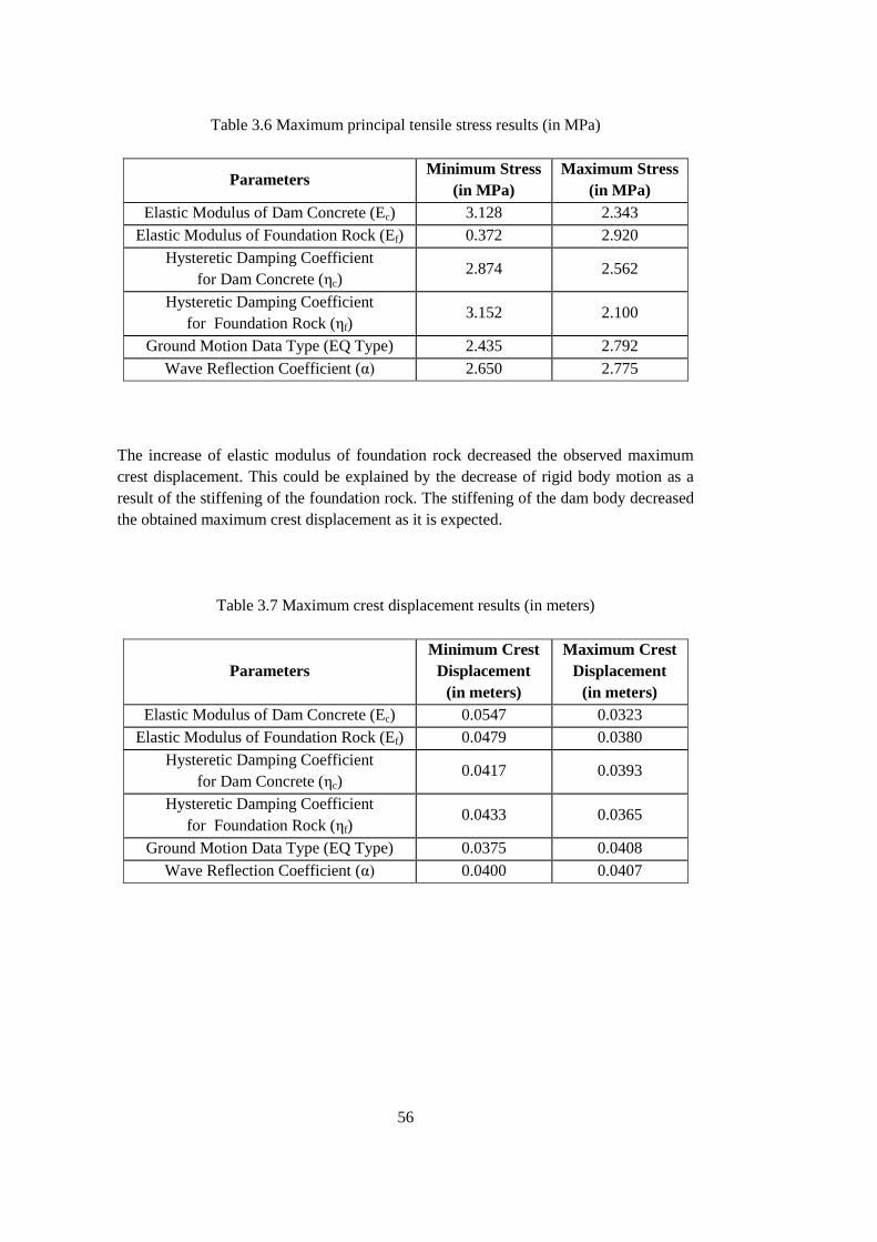
Table 3.6 Maximum principal tensile stress results (in MPa)......................................... 56
Table 3.7 Maximum crest displacement results (in meters) ........................................... 56
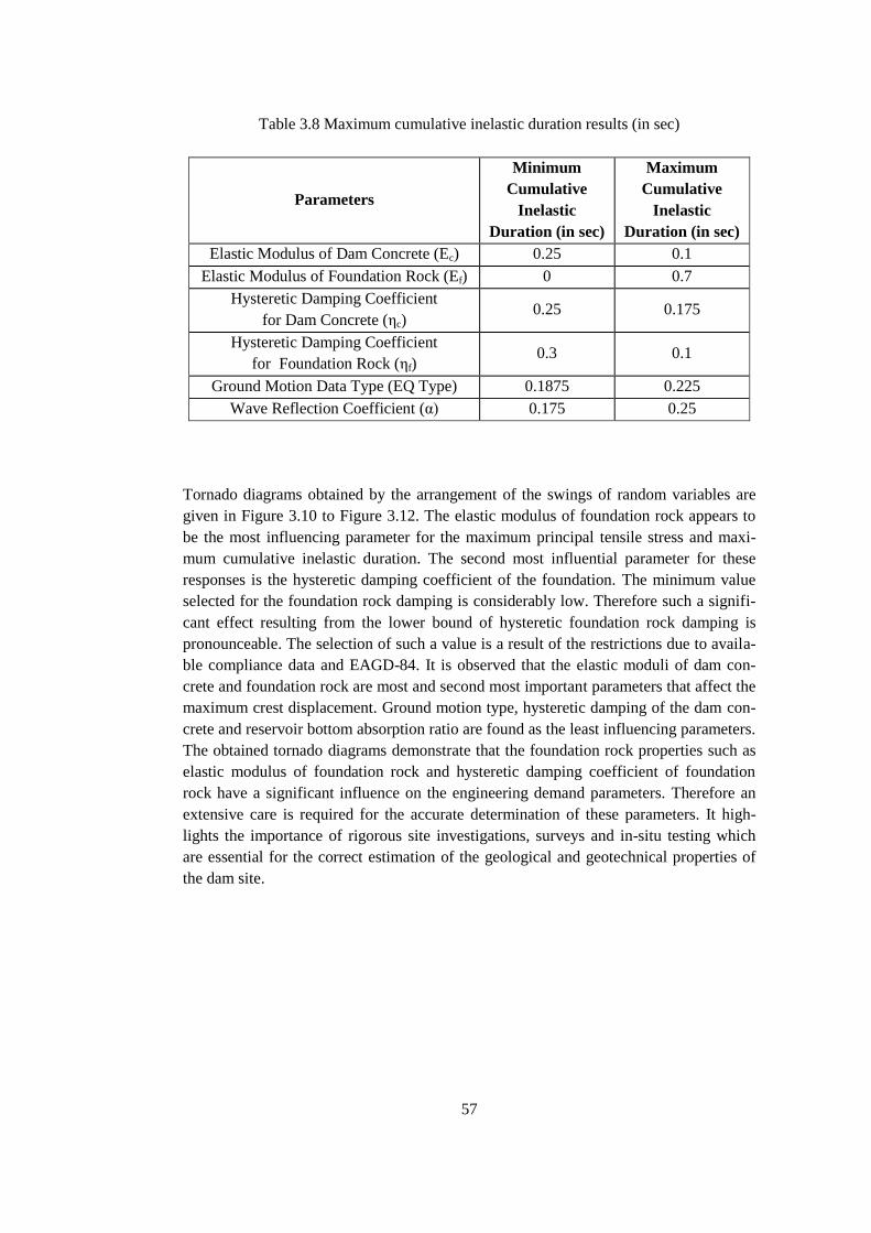
Table 3.8 Maximum cumulative inelastic duration results (in sec) ................................ 57
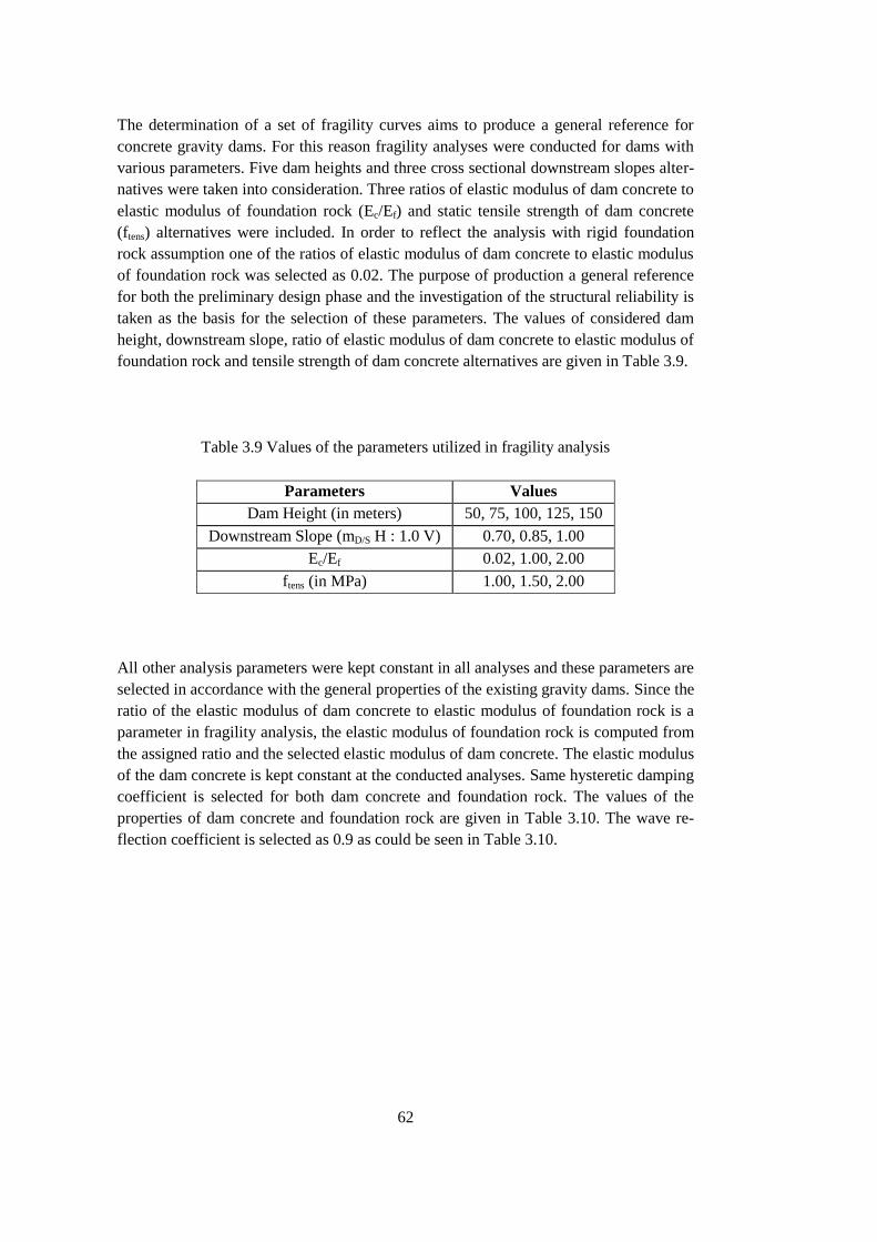
Table 3.9 Values of the parameters utilized in fragility analysis .................................... 62
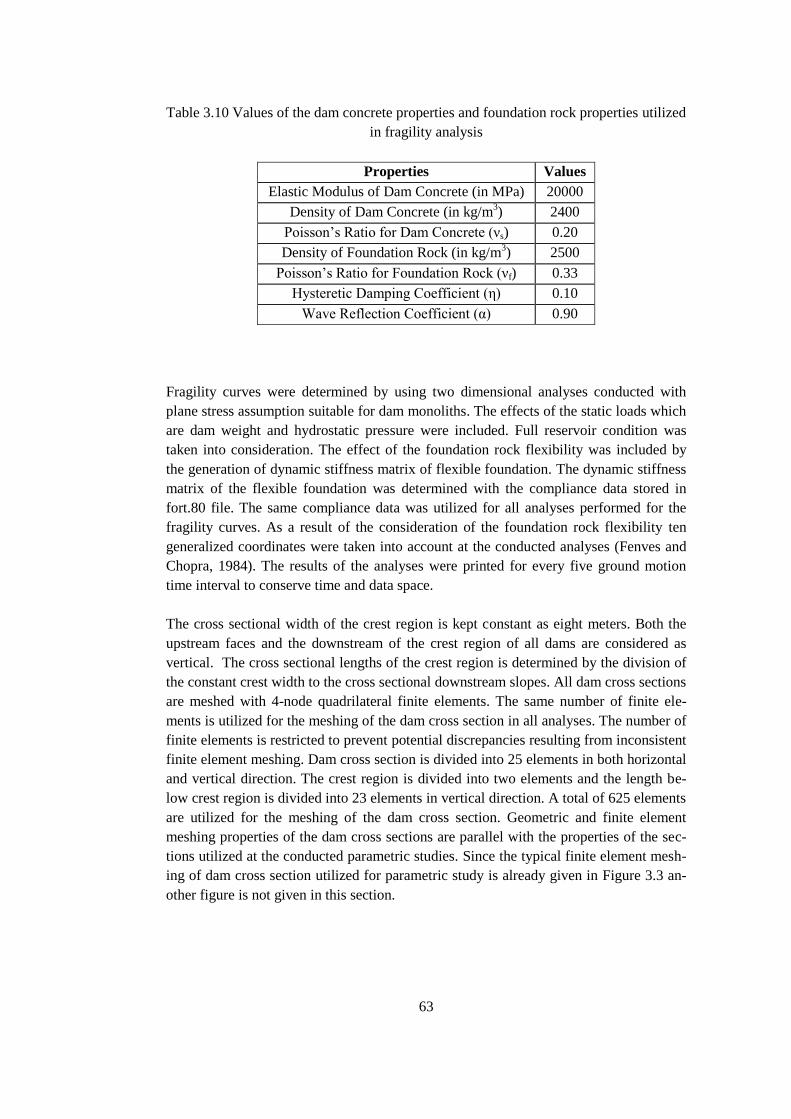
Table 3.10 Values of the dam concrete properties and foundation rock properties utilized
in fragility analysis.......................................................................................................... 63
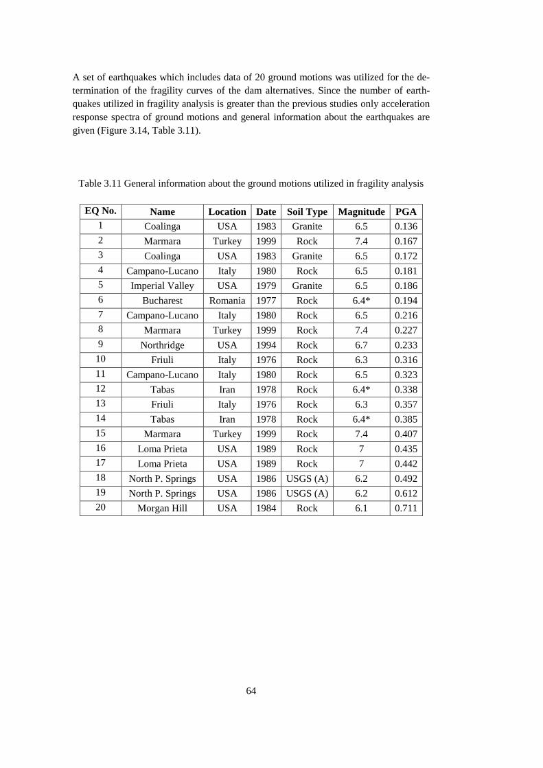
Table 3.11 General information about the ground motions utilized in fragility analysis 64
Page 12
xii
LIST OF FIGURES
FIGURES
Figure 1.1 Cumulative installed capacities of hydroelectic power plants and total
installed capacity in Turkey (World Energy Council Turkish National Committee, 2012)
........................................................................................................................................... 1
Figure 1.2 Distribution of the added mass of virtual water body ...................................... 3
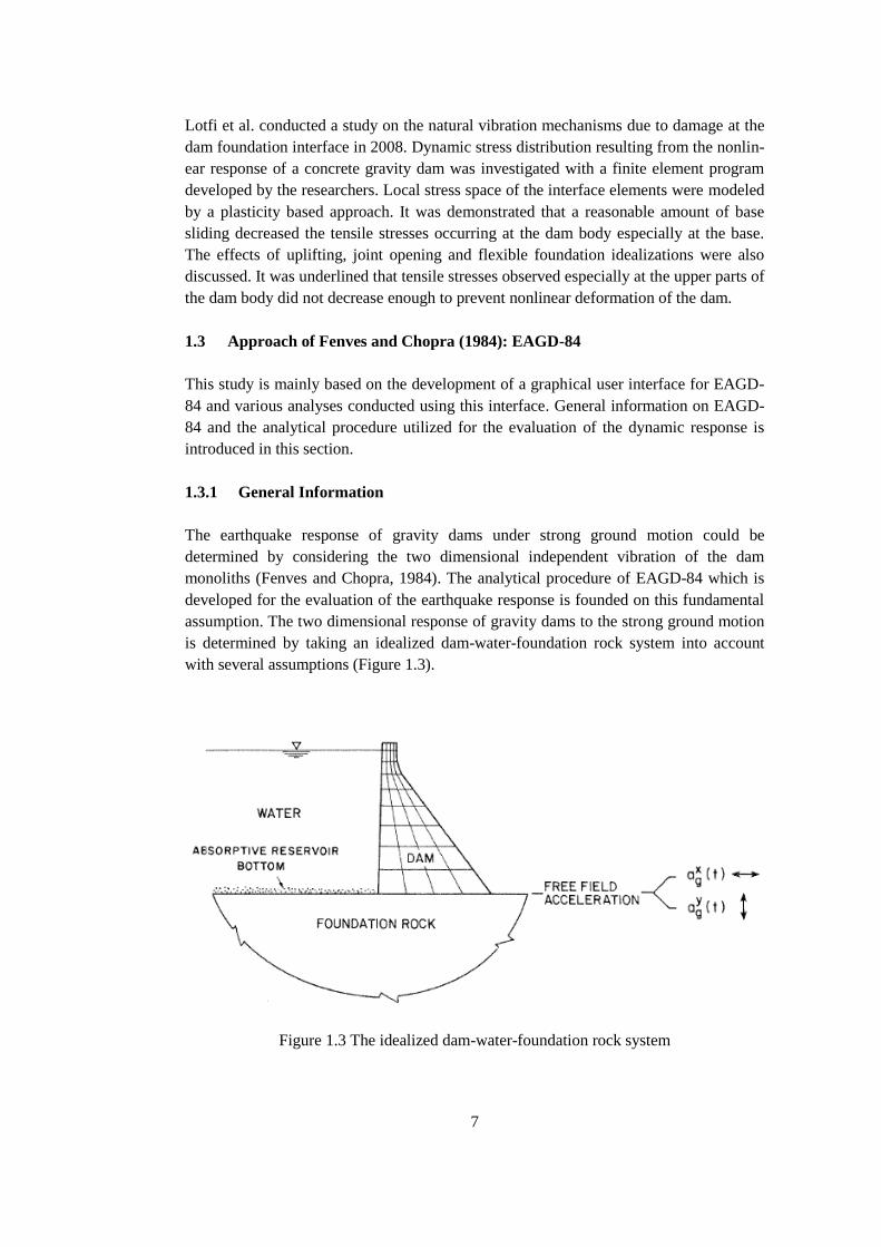
Figure 1.3 The idealized dam-water-foundation rock system ........................................... 7
Figure 1.4 Substructures of the dam-reservoir-foundation rock system ........................... 9
Figure 1.5 Analysis procedure of EAGD-84 ................................................................... 16
Figure 1.6 Stress distribution through dam base of case 1 .............................................. 19
Figure 1.7 Stress distribution through dam base of case 2 .............................................. 19
Figure 1.8 Stress distribution through dam base of case 3 .............................................. 19
Figure 1.9 Stress distribution through dam base of case 4 .............................................. 19
Figure 2.1 A screen capture of graphical user interface of EAGD ModPro ................... 22
Figure 2.2 A screen capture of material properties section from GUI of EAGD ModPro
......................................................................................................................................... 23
Figure 2.3 A screen capture of foundation rock properties section from GUI of EAGD
ModPro ............................................................................................................................ 24
Figure 2.4 The typical dam cross section and a screen capture of geometric properties of
dam section from GUI of EAGD ModPro ...................................................................... 25
Figure 2.5 A screen capture of dynamic response parameters section from GUI of
EAGD ModPro ................................................................................................................ 27
Figure 2.6 A screen capture of analysis output parameters section from GUI of EAGD
ModPro ............................................................................................................................ 29
Figure 2.7 A screen capture of analysis execution parameters section from GUI of
EAGD ModPro ................................................................................................................ 30
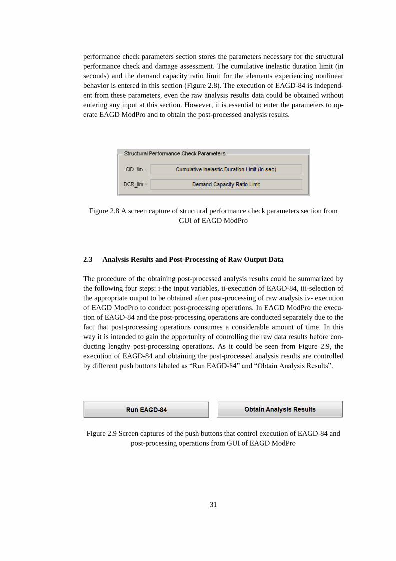
Figure 2.8 A screen capture of structural performance check parameters section from
GUI of EAGD ModPro ................................................................................................... 31
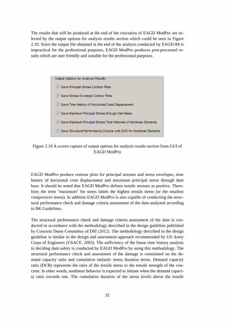
Figure 2.9 Screen captures of the push buttons that control execution of EAGD-84 and
post-processing operations from GUI of EAGD ModPro ............................................... 31
Figure 2.10 A screen capture of output options for analysis results section from GUI of
EAGD ModPro ................................................................................................................ 32
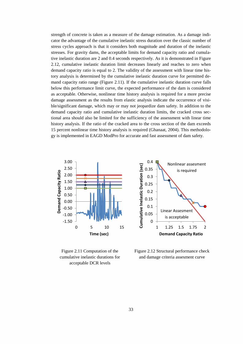
Figure 2.11 Computation of the cumulative inelastic durations for acceptable DCR
levels ............................................................................................................................... 33
Figure 2.12 Structural performance check and damage criteria assesment curve ........... 33
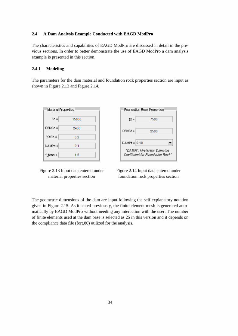
Figure 2.13 Input data entered under material properties section ................................... 34
Figure 2.14 Input data entered under foundation rock properties section ....................... 34
Page 13
xiii
Figure 2.15 Input data entered under geometric properties of dam section and the typical
dam cross section ............................................................................................................ 35
Figure 2.16 Horizontal earthquake ground motion utilized for dam analysis example .. 35
Figure 2.17 Input data entered under dynamic response parameters section .................. 35
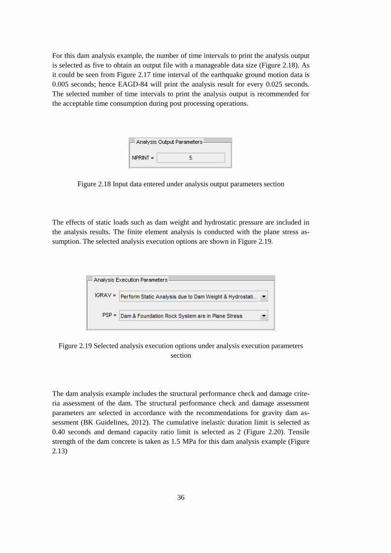
Figure 2.18 Input data entered under analysis output parameters section ...................... 36
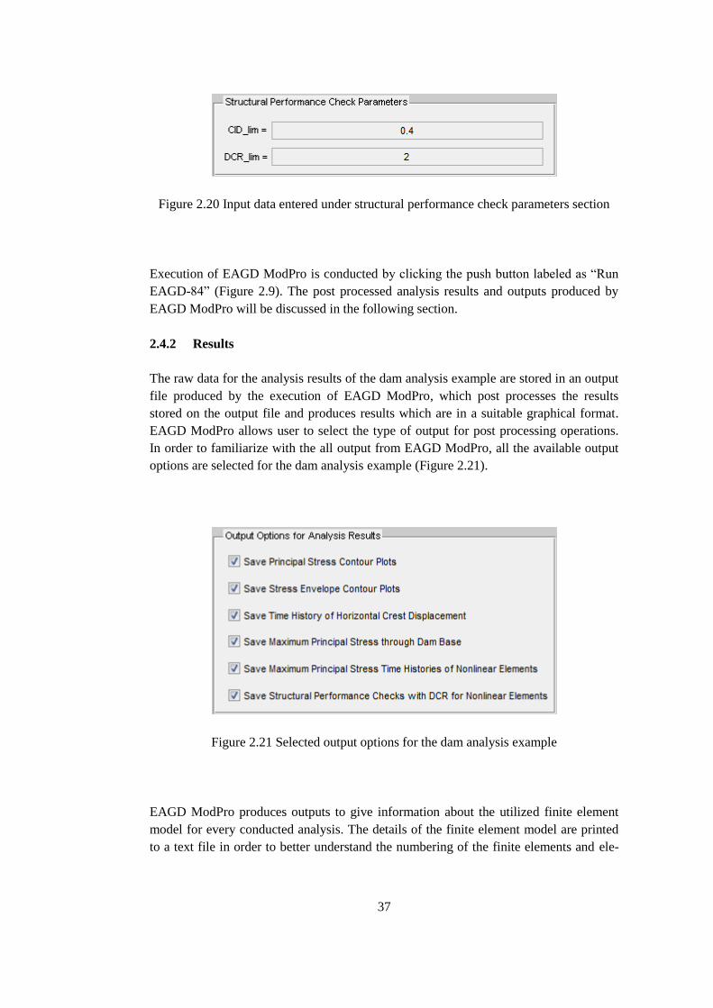
Figure 2.19 Selected analysis execution options under analysis execution parameters
section ............................................................................................................................. 36
Figure 2.20 Input data entered under structural performance check parameters section 37
Figure 2.21 Selected output options for the dam analysis example ................................ 37
Figure 2.22 A screen capture from the text file which includes the detials of the finite
element meshing properties ............................................................................................ 38
Figure 2.23 The finete element meshing of the dam cross section ................................. 38
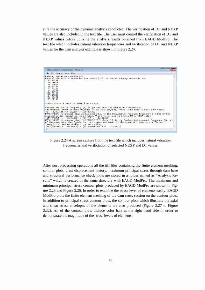
Figure 2.24 A screen capture from the text file which includes natural vibration
frequencies and verificiation of selected NEXP and DT values ..................................... 39
Figure 2.25 Maximum principal stress contour plot ....................................................... 40
Figure 2.26 Minimum principal stress contour plot ........................................................ 40
Figure 2.27 Maximum sigma-x envelope contour plot ................................................... 40
Figure 2.28 Minimum sigma-x envelope contour plot ................................................... 40
Figure 2.29 Maximum sigma-y envelope contour plot ................................................... 40
Figure 2.30 Minimum sigma-y envelope contour plot ................................................... 40
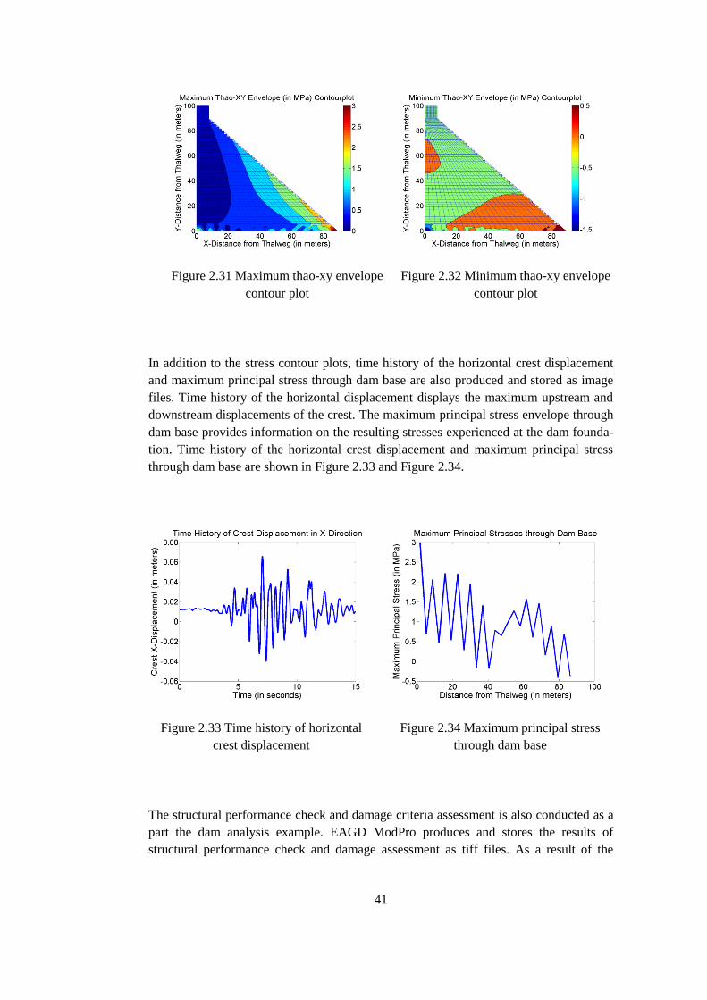
Figure 2.31 Maximum thao-xy envelope contour plot ................................................... 41
Figure 2.32 Minimum thao-xy envelope contour plot .................................................... 41
Figure 2.33 Time history of horizontal crest displacement ............................................ 41
Figure 2.34 Maximum principal stress through dam base .............................................. 41
Figure 2.35 Maximum principal stress time history of the thalweg element .................. 42
Figure 2.36 Cumulative inelastic duration curve of the thalweg element....................... 42
Figure 2.37 Message window which shows the ratio of the cracked area to the dam cross
section ............................................................................................................................. 42
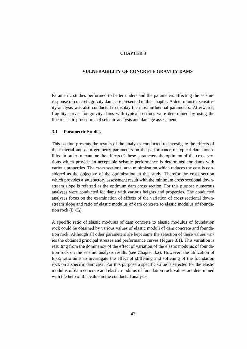
Figure 3.1 Maximum principal stress contourplots and structural performance curves of
dams with the same Ec/Ef ratio (with different values of elastic moduli) ....................... 44
Figure 3.2 Acceleration time history and acceleration response spectrum of the proposed
synthetic ground motion ................................................................................................. 45
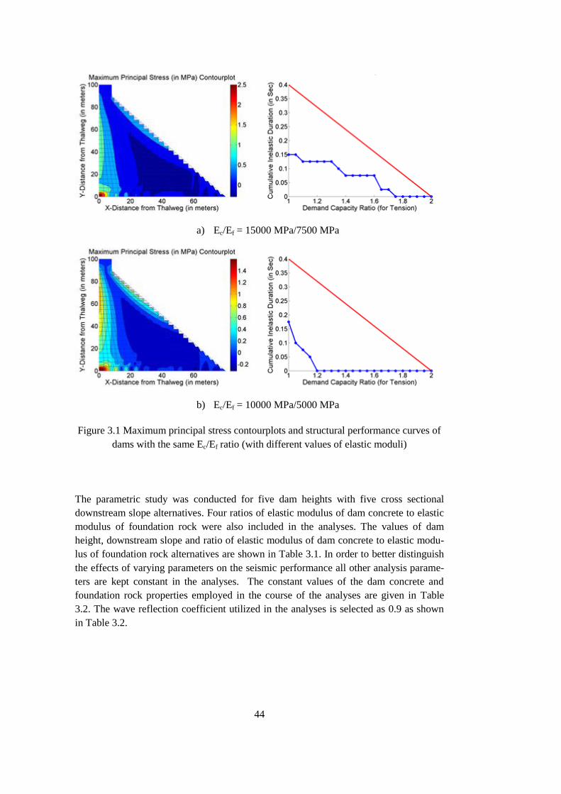
Figure 3.3 Typical dam meshing utilized in the parametric study .................................. 47
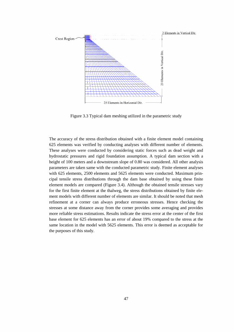
Figure 3.4 Maximum principal stresses through dam base obtained by different finite
element models ............................................................................................................... 48
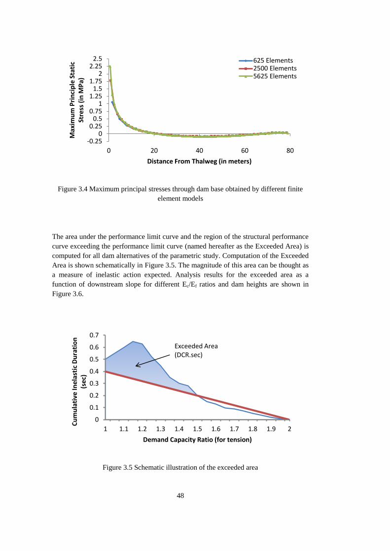
Figure 3.5 Schematic illustration of the exceeded area .................................................. 48
Figure 3.6 The parametric study results for the thalweg elements of analyzed dams .... 49
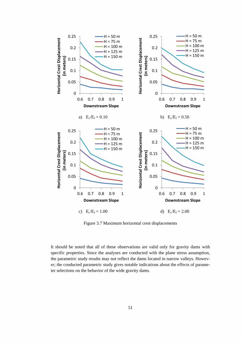
Figure 3.7 Maximum horizontal crest displacements ..................................................... 51
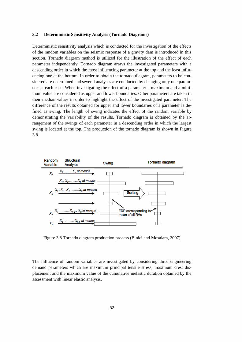
Figure 3.8 Tornado diagram production process (Binici and Mosalam, 2007) .............. 52
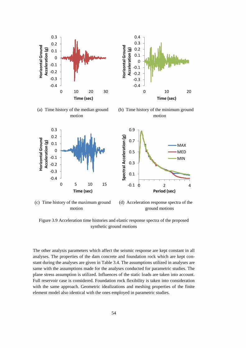
Figure 3.9 Acceleration time histories and elastic response spectra of the proposed
synthetic ground motions ................................................................................................ 54
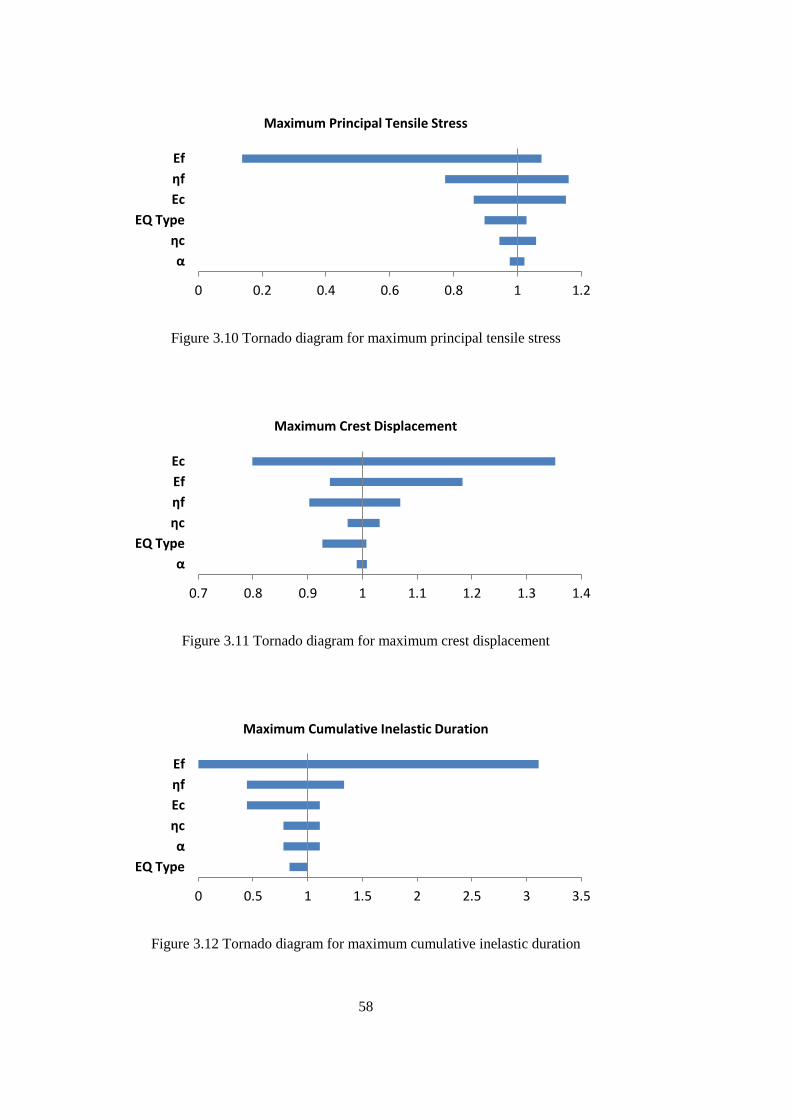
Figure 3.10 Tornado diagram for maximum principal tensile stress .............................. 58
Figure 3.11 Tornado diagram for maximum crest displacement .................................... 58
Figure 3.12 Tornado diagram for maximum cumulative inelastic duration ................... 58
Page 14
xiv
Figure 3.13 The procedure of the determination of a fragility curve .............................. 61
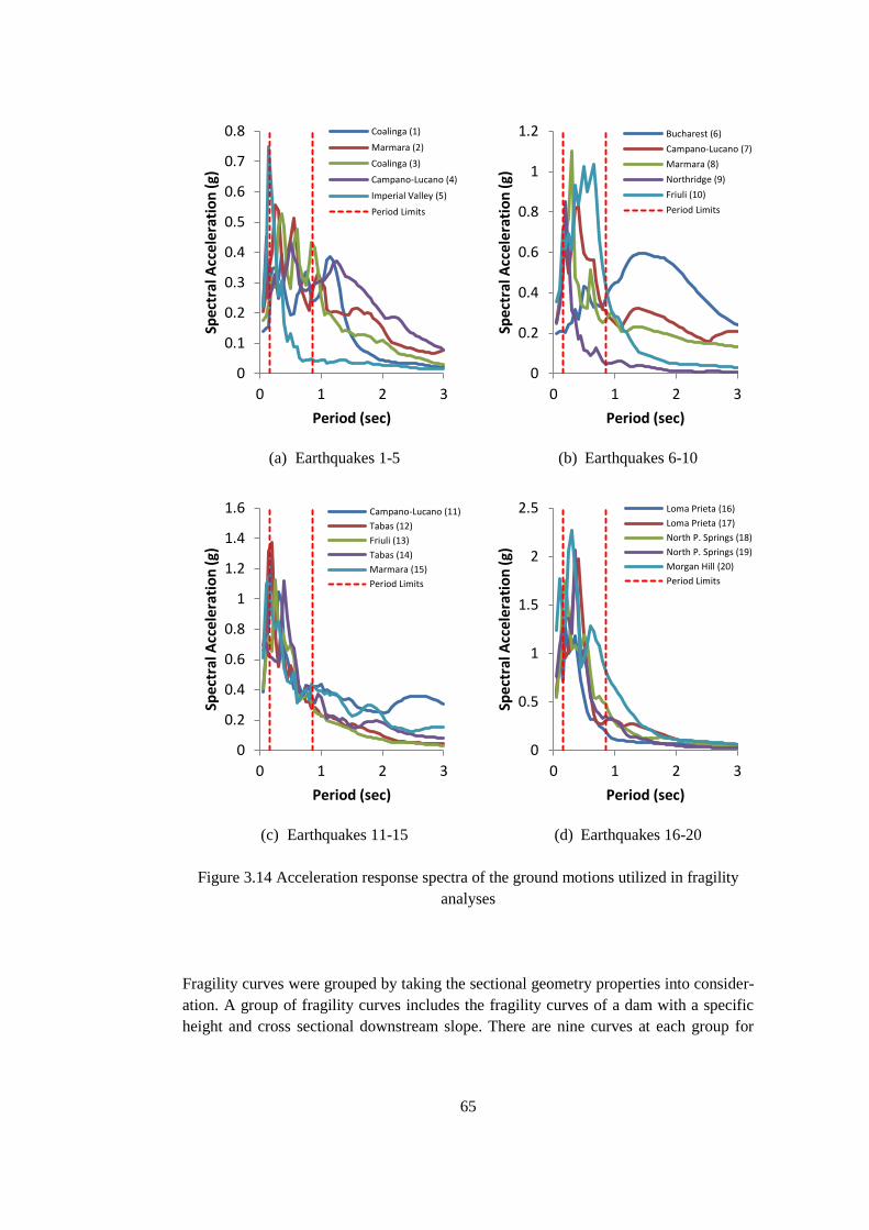
Figure 3.14 Acceleration response spectra of the ground motions utilized in fragility
analyses ........................................................................................................................... 65
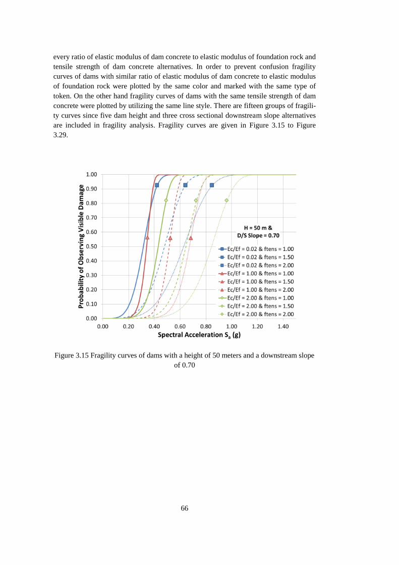
Figure 3.15 Fragility curves of dams with a height of 50 meters and a downstream slope
of 0.70 ............................................................................................................................. 66
Figure 3.16 Fragility curves of dams with a height of 50 meters and a downstream slope
of 0.85 ............................................................................................................................. 67
Figure 3.17 Fragility curves of dams with a height of 50 meters and a downstream slope
of 1.00 ............................................................................................................................. 67
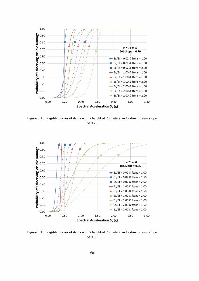
Figure 3.18 Fragility curves of dams with a height of 75 meters and a downstream slope
of 0.70 ............................................................................................................................. 68
Figure 3.19 Fragility curves of dams with a height of 75 meters and a downstream slope
of 0.85 ............................................................................................................................. 68
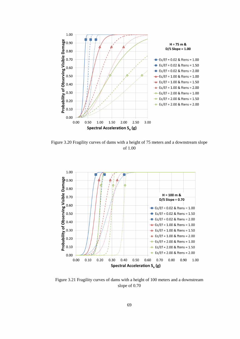
Figure 3.20 Fragility curves of dams with a height of 75 meters and a downstream slope
of 1.00 ............................................................................................................................. 69
Figure 3.21 Fragility curves of dams with a height of 100 meters and a downstream
slope of 0.70 .................................................................................................................... 69
Figure 3.22 Fragility curves of dams with a height of 100 meters and a downstream
slope of 0.85 .................................................................................................................... 70
Figure 3.23 Fragility curves of dams with a height of 100 meters and a downstream
slope of 1.00 .................................................................................................................... 70
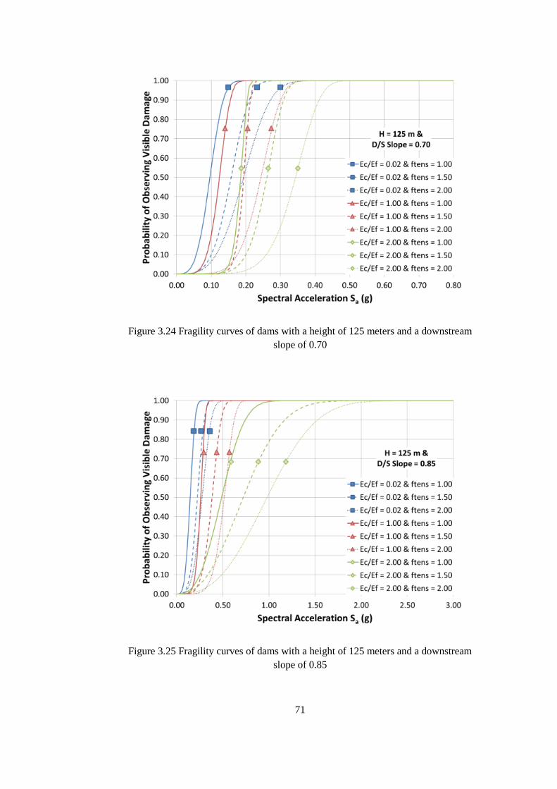
Figure 3.24 Fragility curves of dams with a height of 125 meters and a downstream
slope of 0.70 .................................................................................................................... 71
Figure 3.25 Fragility curves of dams with a height of 125 meters and a downstream
slope of 0.85 .................................................................................................................... 71
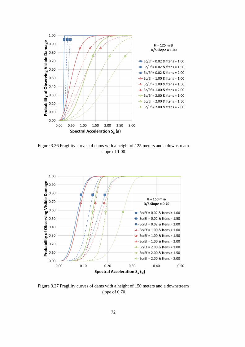
Figure 3.26 Fragility curves of dams with a height of 125 meters and a downstream
slope of 1.00 .................................................................................................................... 72
Figure 3.27 Fragility curves of dams with a height of 150 meters and a downstream
slope of 0.70 .................................................................................................................... 72
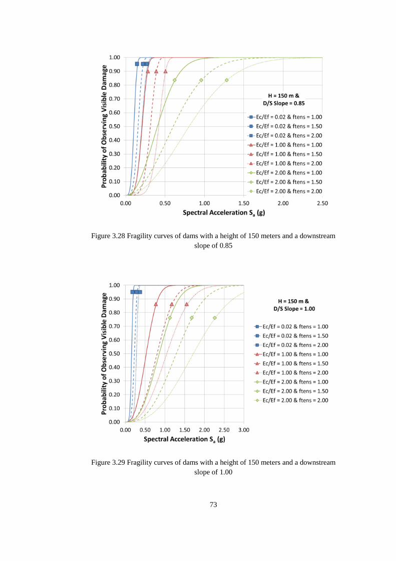
Figure 3.28 Fragility curves of dams with a height of 150 meters and a downstream
slope of 0.85 .................................................................................................................... 73
Figure 3.29 Fragility curves of dams with a height of 150 meters and a downstream
slope of 1.00 .................................................................................................................... 73
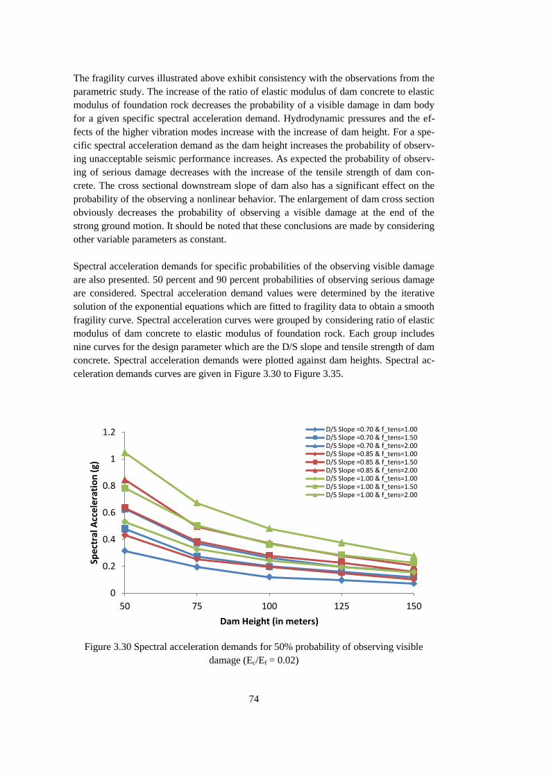
Figure 3.30 Spectral acceleration demands for 50% probability of observing visible
damage (Ec/Ef = 0.02)...................................................................................................... 74
Figure 3.31 Spectral acceleration demands for 50% probability of observing visible
damage (Ec/Ef = 1.00) .................................................................................................... 75
Figure 3.32 Spectral acceleration demands for 50% probability of observing visible
damage (Ec/Ef = 2.00) .................................................................................................... 75
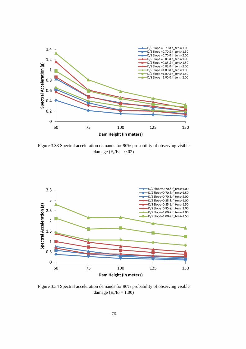
Figure 3.33 Spectral acceleration demands for 90% probability of observing visible
damage (Ec/Ef = 0.02)...................................................................................................... 76
Figure 3.34 Spectral acceleration demands for 90% probability of observing visible
damage (Ec/Ef = 1.00)...................................................................................................... 76
Page 15
xv
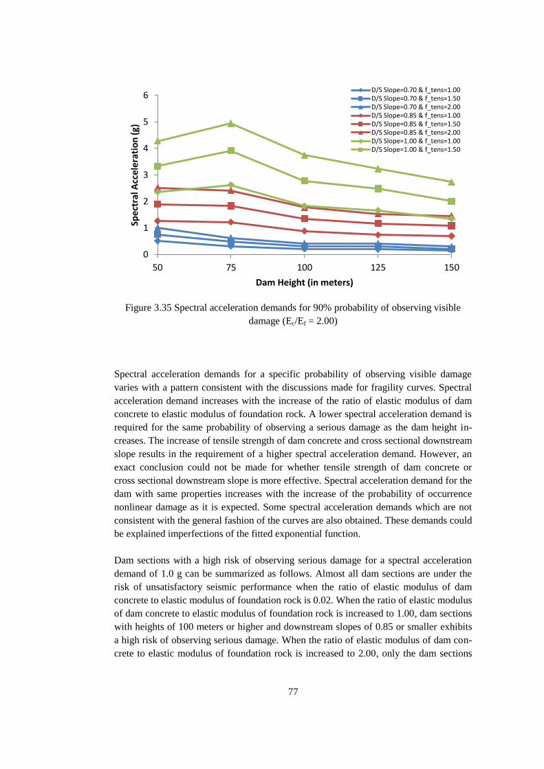
Figure 3.35 Spectral acceleration demands for 90% probability of observing visible
damage (Ec/Ef = 2.00) ..................................................................................................... 77
Page 17
1
CHAPTER 1
1 INTRODUCTION
1.1 General
The energy demand in Turkey has risen significantly as a result of the industrial devel-
opments and increase in population within the last decades. The sharp increase of the
energy demand forces Turkey to utilize all available energy production options. In order
to satisfy the supply demand equilibrium for energy, a large number of power plants are
constructed and taken into operation. The majority of these power plants are natural gas
power plants and natural gas combined cycle power plants. As a result of the increase in
the number of power plants utilizing non-domestic natural resources, foreign resource
dependent energy production becomes one of the most crucial problems of Turkey. This
critical situation makes utilization of domestic sources for energy production important
for Turkey.
The dramatic increase in energy demand and current dependence on the petroleum based
energy production requires utilization of hydroelectric power an important option as a
domestic, clean and reliable energy source. In addition to the increase in energy demand,
irrigation and water demand also increase with the population growth. The aggregation
of these factors results in a trend of dam construction in Turkey. This trend gained mo-
mentum, especially in the last decade, with the legislation which opened the doors of the
energy production to private sector. The sharp increase of the cumulative installed ca-
pacities of hydroelectric power plants and at the total installed capacity is shown in Fig-
ure 1.1.
Figure 1.1 Cumulative installed capacities of hydroelectic power plants and total
installed capacity in Turkey (World Energy Council Turkish National Committee, 2012)
0
12500
25000
37500
50000
1950 1960 1970 1980 1990 2000 2010
Inst
alle
d
Cap
acit
y (M
W)
Year
Hydroelectric Power Plants
Total Capacity
Page 18
2
The number of dams constructed by the private hydroelectricity companies is about 600.
A significant number of dams are constructed or at the construction phase as a result of
this. It is also planned to construct a large number of dams in the following years. Use of
roller compacted concrete, as an alternative to conventionally vibrated concrete, increas-
es the attractiveness of the concrete gravity dams by decreasing the construction dura-
tion and costs. Despite the recent advancements in the dam construction sector, the his-
tory of modern concrete gravity dam construction dates back to the first years of the
Turkish Republic. Çubuk I Dam, which is the first concrete arch gravity dam of Turkey
was taken into operation in 1936, interestingly at a similar date to that of Hoover Dam.
Following the Çubuk I Dam a number of concrete gravity dams were constructed in the
following approximately 20 years. Some of these dams with their construction dates are
Porsuk I Dam (1948), Elmanlı II Dam (1955), Sarıyar Dam (1956) and Kemer Dam
(1958) (Öziş, 1990).
Turkey lies at the intersection of a number of major and minor active faults, hence she is
in a seismic prone region with severe earthquake risk. Dams are special and monumental
type of structures requiring extensive care at their seismic design stage. Therefore mod-
ern analysis and design techniques must be utilized in today’s computer age. In addition
to the need of modern tools for seismic design of new dams, methods for the seismic
damage assessment of old dams are also needed. A concrete step for the recommenda-
tion of modern seismic design and analysis principles is taken by the general directorate
of state hydraulic works. Dams Congress is organized by the general directorate of state
hydraulic works in 2012 and design guidelines were formed as a result of collaboration
of the academicians and professionals. The procedures proposed by these guidelines
(BK Guidelines, 2012) are taken as a basis for the conducted studies in this work.
1.2 Literature Survey
The seismic behavior of concrete gravity dams under strong ground motion is investi-
gated by numerous researchers in the past. Various assumptions and simplifications
were made to simulate the dynamic behavior of the dam-reservoir-foundation rock sys-
tem. Although these assumptions may cause deviations from the actual seismic behavior
of the dam, better estimations of the seismic response of the dams is achieved in time by
the efforts of researchers. The most critical research available in the literature is the
studies focused on the evaluation of hydrodynamic pressures, dam-reservoir-foundation
rock interactions and reservoir bottom absorption.
The pioneer of the research on the response of the dams under earthquake acceleration
dates back to study presented by Westergaard in 1933. In order to determine the hydro-
dynamic pressures resulting from a strong ground motion, a straight and rigid dam body
with a vertical upstream face and an infinite reservoir was considered. Only the horizon-
tal component of the ground motion was taken into account and the compressibility of
the water was included. Resulting displacements were assumed to be small and the ef-
fects of the surface waves were ignored. The effects of hydrodynamic pressures was
Page 19
3
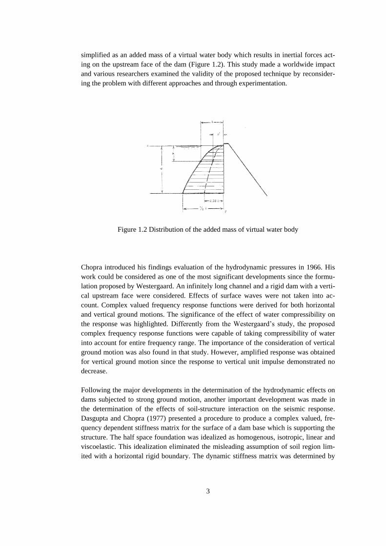
simplified as an added mass of a virtual water body which results in inertial forces act-
ing on the upstream face of the dam (Figure 1.2). This study made a worldwide impact
and various researchers examined the validity of the proposed technique by reconsider-
ing the problem with different approaches and through experimentation.
Figure 1.2 Distribution of the added mass of virtual water body
Chopra introduced his findings evaluation of the hydrodynamic pressures in 1966. His
work could be considered as one of the most significant developments since the formu-
lation proposed by Westergaard. An infinitely long channel and a rigid dam with a verti-
cal upstream face were considered. Effects of surface waves were not taken into ac-
count. Complex valued frequency response functions were derived for both horizontal
and vertical ground motions. The significance of the effect of water compressibility on
the response was highlighted. Differently from the Westergaard’s study, the proposed
complex frequency response functions were capable of taking compressibility of water
into account for entire frequency range. The importance of the consideration of vertical
ground motion was also found in that study. However, amplified response was obtained
for vertical ground motion since the response to vertical unit impulse demonstrated no
decrease.
Following the major developments in the determination of the hydrodynamic effects on
dams subjected to strong ground motion, another important development was made in
the determination of the effects of soil-structure interaction on the seismic response.
Dasgupta and Chopra (1977) presented a procedure to produce a complex valued, fre-
quency dependent stiffness matrix for the surface of a dam base which is supporting the
structure. The half space foundation was idealized as homogenous, isotropic, linear and
viscoelastic. This idealization eliminated the misleading assumption of soil region lim-
ited with a horizontal rigid boundary. The dynamic stiffness matrix was determined by
Page 20
4
utilizing the influence coefficients of the surface of a viscoelastic half space in plane
stress or plane strain. The influence coefficients were obtained by solving two boundary
value problems with prescribed harmonically time varying normal and shear stresses
which are distributed uniformly over a surface element. It was shown that the introduced
procedure increases the accuracy of the produced dynamic stiffness matrix. The compat-
ibility of displacements at nodal points and equilibrium of stresses were also ensured
with the proposed method.
Fenves and Chopra developed a semi analytical-numerical procedure to analyze the
earthquake response of concrete gravity dams in 1984. The effects of dam-reservoir-
foundation rock interaction and sediments accumulated at reservoir bottom were includ-
ed with substructure method in this study. The effects of the reservoir bottom materials
were discussed for a simplified system at first. The flexibility of foundation rock was
neglected by rigid foundation assumption and only the fundamental vibration mode was
taken into account in the first part of the work. Both the horizontal and vertical compo-
nents of the ground motion were taken into consideration. The absorptive effect of the
reservoir bottom materials was reflected by a boundary condition which dissipates a
portion of the hydrodynamic pressure waves. The results of simplified system demon-
strated that the absorptive reservoir bottom materials have a major effect on the earth-
quake response. A general analytical procedure which includes the dam-reservoir-
foundation rock interaction and the reservoir bottom absorption effects was developed
next by improving the considered simplified system. Effects of all significant modes and
flexibility of the foundation rock were taken into account in the proposed procedure.
Continuum solutions for the foundation and numerical evaluation methods for the dam
body were discussed. The earthquake response of an idealized concrete gravity dam was
investigated by utilizing the developed general procedure. The response of the dam sub-
jected to a harmonic ground motion was found for a wide range of design parameters
and the results were presented in the form of frequency response functions. The obtained
frequency response functions proved that the effect of absorptive reservoir bottom was
important. The tallest non-overflow monolith of Pine Flat concrete gravity dam was
analyzed under the Taft ground motion. Several assumptions for the reservoir and foun-
dation rock and various ratios of reservoir bottom absorption were considered. Horizon-
tal and vertical components of the Taft ground motion was taken into account. The anal-
yses results demonstrated that the dam-reservoir and dam-foundation rock interactions
and the reservoir bottom absorption had a significant influence on the resulting stresses
and displacements. The importance of considering the vertical component of the ground
motion was also observed from the results. Finally a simplified method was developed
for the preliminary design and safety assessment of concrete gravity dams. The pro-
posed method considered an equivalent single degree of freedom system for approxi-
mate representation of the dam behavior. The results obtained by the simplified method
were independent from the excitation frequency. Only the fundamental mode response
to horizontal ground motion was taken into account.
Page 21
5
A computer program named as EAGD-84 was prepared by Fenves and Chopra in 1984.
EAGD-84 was developed for the numerical evaluation of the earthquake response of the
dams by utilizing the proposed procedure. The dam cross section was idealized as a two
dimensional finite element system. Stress and displacement response histories of dams
were obtained as the fundamental result of the analyses. The details of the proposed
analytical procedure and EAGD-84 are described in the following section.
Lotfi et al. presented an alternative study to Fenves and Chopra’s work in 1987. The
major difference of the developed technique was its approach to the reservoir water-
flexible foundation interaction. The water-foundation interaction was considered by
enforcing stress and displacement continuity normal to reservoir foundation interface.
The developed hyper-element technique was capable of considering layered founda-
tions. Analysis of an idealized dam-foundation-reservoir system with the proposed tech-
nique was presented. The results of the conducted analyses were discussed and the effi-
ciency of the developed technique in the consideration of the reservoir-foundation inter-
action was introduced.
Effect of reservoir-foundation interaction was the subject of a study conducted by
Dominguez et al (1990). A boundary integral technique was proposed for the investiga-
tion of the response of dam-reservoir-sediment-foundation systems subjected to ground
acceleration. The boundary element method was utilized for the development of the
proposed technique. The study took both the viscoelastic half plane and layered founda-
tion assumptions into consideration. The effects of the foundation flexibility, full and
empty reservoir cases and the existence of the sediment layer were investigated. The
results were compared with the previous studies conducted by Fenves and Chopra
(1984) and Lotfi et al (1987). The results of the majority of the cases were consistent
with the previous studies. The most significant inconsistency was observed at the full
reservoir with viscoelastic half space foundation case. This inconsistency was intro-
duced as a result of the exaggerated damping arising from the boundary condition of
absorptive reservoir bottom proposed by Fenves and Chopra.
Bougacha et al. introduced a technique based on the finite element method for the analy-
sis of wave generation in a layered, fluid filled poroelastic media to consider the sedi-
ments in 1993. The wave motion was considered as the combination of the modes which
are continuous in horizontal and vertical directions. The plane strain and antiplane shear
deformations were taken into account. Deformations in both plane and axisymmetric
regions were considered and consistent transmitting boundaries were formulated for
these regions. The application of the developed technique was given in a companion
study. The dynamic stiffness matrices of strip and circular foundations with a rigid sur-
face were determined. In addition to the application of the developed technique a simpli-
fied method for the determination of the dynamic stiffness matrix was also presented.
The simplified method assumed an equivalent solid for the representation of the two
phase medium. It was demonstrated that the accuracy of the approximate method is sat-
isfactory especially for the low frequency range.
Page 22
6
The studies presented above concentrated on the evaluation of the dynamic response of
dams by taking dam-reservoir-foundation rock interactions and the effects of reservoir
bottom materials into consideration. The focus of the researchers has been shifted to the
nonlinear analysis and assessment of dams towards the end of 20th century.
Bhattacharjee et al. conducted a study on the two dimensional static fracture behavior of
dams in 1994. Smeared crack models were developed from a nonlinear fracture mechan-
ics point of view that can simulate the tensile and shear softening of the plain concrete.
A coaxial rotating crack model and a fixed crack model with a variable shear resistance
factor were presented. The nonlinear analyses of a notched shear beam, a model and a
full scale concrete gravity dams were conducted by the proposed crack models. The
results were compared with the experimental and analytical results presented by the
previous researchers. It was shown that the both models give satisfactory results for full
scale concrete gravity dams.
The static fracture behavior of a dam subjected to an incremental increase of the reser-
voir water level was also investigated by Bhattacharjee et al. in 1995. A rotating
smeared crack model was considered in the nonlinear finite element analyses. The uplift
pressure occurring inside the smeared crack bands was taken into account by effective
porosity concept. The analyses results obtained by finite element analyses and conven-
tional no-tension gravity method were compared. The fracture analysis of dams was
recommended for the safety evaluation of dams since it was observed that the usage of
gravity method might give results on the unsafe side.
Ghanaat introduced a method for the seismic performance evaluation of dams in 2004.
The proposed assessment approach utilized linear time history analyses. The potential
failure mechanisms of concrete gravity, buttress and arch dams were discussed and tak-
en into consideration at the introduced performance evaluation approach. The perfor-
mance evaluation procedure took magnitudes of demand capacity ratios, cumulative
duration of inelastic stresses and magnitude of the cracked area into account. The crite-
ria for the sufficiency of linear elastic analyses were introduced. The effectiveness of the
proposed performance evaluation approach was demonstrated with linear and nonlinear
analyses.
Javanmardi et al. developed a theoretical method to determine the water pressure varia-
tions along a tensile crack during dynamic response in 2005. The results of the proposed
model were compared with experimental test results. It was demonstrated that reservoir
water enters the crack and a certain length of the crack become partially saturated. Finite
element analyses of a 90 meters high gravity dam were conducted. The uplift pressure
inside the crack was decreased with crack opening and increased with crack closing. It
was noted that crack opening does not affect the downstream sliding safety factor. Since
the excessive water pressure mainly occurs close the crack mouth crack closing mecha-
nism also did not pose a serious threat to the sliding safety.
Page 23
7
Lotfi et al. conducted a study on the natural vibration mechanisms due to damage at the
dam foundation interface in 2008. Dynamic stress distribution resulting from the nonlin-
ear response of a concrete gravity dam was investigated with a finite element program
developed by the researchers. Local stress space of the interface elements were modeled
by a plasticity based approach. It was demonstrated that a reasonable amount of base
sliding decreased the tensile stresses occurring at the dam body especially at the base.
The effects of uplifting, joint opening and flexible foundation idealizations were also
discussed. It was underlined that tensile stresses observed especially at the upper parts of
the dam body did not decrease enough to prevent nonlinear deformation of the dam.
1.3 Approach of Fenves and Chopra (1984): EAGD-84
This study is mainly based on the development of a graphical user interface for EAGD-
84 and various analyses conducted using this interface. General information on EAGD-
84 and the analytical procedure utilized for the evaluation of the dynamic response is
introduced in this section.
1.3.1 General Information
The earthquake response of gravity dams under strong ground motion could be
determined by considering the two dimensional independent vibration of the dam
monoliths (Fenves and Chopra, 1984). The analytical procedure of EAGD-84 which is
developed for the evaluation of the earthquake response is founded on this fundamental
assumption. The two dimensional response of gravity dams to the strong ground motion
is determined by taking an idealized dam-water-foundation rock system into account
with several assumptions (Figure 1.3).
Figure 1.3 The idealized dam-water-foundation rock system
Page 24
8
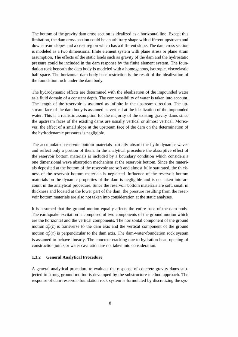
The bottom of the gravity dam cross section is idealized as a horizontal line. Except this
limitation, the dam cross section could be an arbitrary shape with different upstream and
downstream slopes and a crest region which has a different slope. The dam cross section
is modeled as a two dimensional finite element system with plane stress or plane strain
assumption. The effects of the static loads such as gravity of the dam and the hydrostatic
pressure could be included in the dam response by the finite element system. The foun-
dation rock beneath the dam body is modeled with a homogenous, isotropic, viscoelastic
half space. The horizontal dam body base restriction is the result of the idealization of
the foundation rock under the dam body.
The hydrodynamic effects are determined with the idealization of the impounded water
as a fluid domain of a constant depth. The compressibility of water is taken into account.
The length of the reservoir is assumed as infinite in the upstream direction. The up-
stream face of the dam body is assumed as vertical at the idealization of the impounded
water. This is a realistic assumption for the majority of the existing gravity dams since
the upstream faces of the existing dams are usually vertical or almost vertical. Moreo-
ver, the effect of a small slope at the upstream face of the dam on the determination of
the hydrodynamic pressures is negligible.
The accumulated reservoir bottom materials partially absorb the hydrodynamic waves
and reflect only a portion of them. In the analytical procedure the absorptive effect of
the reservoir bottom materials is included by a boundary condition which considers a
one dimensional wave absorption mechanism at the reservoir bottom. Since the materi-
als deposited at the bottom of the reservoir are soft and almost fully saturated, the thick-
ness of the reservoir bottom materials is neglected. Influence of the reservoir bottom
materials on the dynamic properties of the dam is negligible and is not taken into ac-
count in the analytical procedure. Since the reservoir bottom materials are soft, small in
thickness and located at the lower part of the dam; the pressure resulting from the reser-
voir bottom materials are also not taken into consideration at the static analyses.
It is assumed that the ground motion equally affects the entire base of the dam body.
The earthquake excitation is composed of two components of the ground motion which
are the horizontal and the vertical components. The horizontal component of the ground
motion is transverse to the dam axis and the vertical component of the ground
motion is perpendicular to the dam axis. The dam-water-foundation rock system
is assumed to behave linearly. The concrete cracking due to hydration heat, opening of
construction joints or water cavitation are not taken into consideration.
1.3.2 General Analytical Procedure
A general analytical procedure to evaluate the response of concrete gravity dams sub-
jected to strong ground motion is developed by the substructure method approach. The
response of dam-reservoir-foundation rock system is formulated by discretizing the sys-
Page 25
9
tem into three substructures which are dam substructure, foundation rock substructure
and fluid domain substructure (Figure 1.4).
Figure 1.4 Substructures of the dam-reservoir-foundation rock system
The general equation of motion of a two dimensional finite element system of a dam is:
(1.1)
where , and are the mass, damping and stiffness matrices of the dam, rc is the
vector of relative displacements of the nodes, and
are directional unit vectors,
and
are horizontal and vertical ground accelerations respectively, is the force
vector which is composed of forces acting on the upstream face and the base of the dam.
The equation of motion of the dam-foundation rock system is obtained by the partition-
ing of nodal points into nodal points at the base and nodal points above the base. The
equation of motion is written in the frequency domain by considering harmonic ground
accelerations (Equation 1.2).
[ [
] [
]] {
} {
} {
} (1.2)
In Equation 1.2, and represent relative displacement of nodal points above the base
and the nodal points on the base, and
represent hydrodynamic forces on the up-
stream face and dam-foundation interaction forces on the base and represents the
constant hysteretic factor for the dam concrete.
Page 26
10
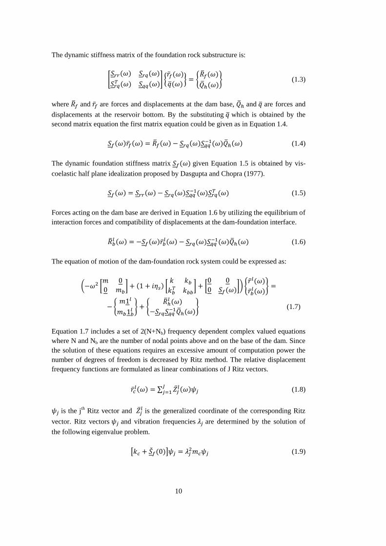
The dynamic stiffness matrix of the foundation rock substructure is:
[
] {
} {
} (1.3)
where and are forces and displacements at the dam base, and are forces and
displacements at the reservoir bottom. By the substituting which is obtained by the
second matrix equation the first matrix equation could be given as in Equation 1.4.
(1.4)
The dynamic foundation stiffness matrix given Equation 1.5 is obtained by vis-
coelastic half plane idealization proposed by Dasgupta and Chopra (1977).
(1.5)
Forces acting on the dam base are derived in Equation 1.6 by utilizing the equilibrium of
interaction forces and compatibility of displacements at the dam-foundation interface.
(1.6)
The equation of motion of the dam-foundation rock system could be expressed as:
( [
] [
] [
]) {
}
{
} {
} (1.7)
Equation 1.7 includes a set of 2(N+Nb) frequency dependent complex valued equations
where N and Nb are the number of nodal points above and on the base of the dam. Since
the solution of these equations requires an excessive amount of computation power the
number of degrees of freedom is decreased by Ritz method. The relative displacement
frequency functions are formulated as linear combinations of J Ritz vectors.
∑
(1.8)
is the jth Ritz vector and
is the generalized coordinate of the corresponding Ritz
vector. Ritz vectors and vibration frequencies are determined by the solution of
the following eigenvalue problem.
[ ] (1.9)
Page 27
11
where
[
] (1.10)
In order to normalize the determined Ritz vectors the equation of is satis-
fied. The following equation is obtained by introducing Equation 1.8 into Equation 1.7,
multiplying the equation by and utilizing the orthogonality properties of eigenvec-
tors.
(1.11)
The elements of the matrix and the vector could be expressed as the following.
[ ]
[ ] (1.12a)
{
}
(1.12b)
The vector includes J number of dynamic frequency response functions for the gen-
eralized coordinates . A sub vector of Ritz vectors which corresponds to nodal points
of the upstream face of dam is represented as and the Kronecker delta function is
represented as .
The complex valued frequency response functions for the hydrodynamic pressures are
obtained by the solution of the two dimensional Helmholtz equation (Equation 1.13).
(1.13)
In the Helmholtz equation represents the frequency response function for hydrody-
namic pressure and represents the velocity of the pressure waves in water. The Helm-
holtz equation is solved for the following boundary conditions:
[ ∑
] (1.14a)
[ ∑
] (1.14b)
(1.14c)
Page 28
12
where
(1.15)
and represents the density of the water. The effects of the absorptive reservoir bottom
materials are taken into account as one dimensional wave absorption. For this purpose
the frequency response function for the vertical displacement at the reservoir bottom is
expressed as following.
(1.16)
The compliance function which represents the absorptive reservoir bottom materi-
als is obtained by the solution of the one dimensional Helmholtz equation:
[
] (1.17)
where √ , and are the elastic modulus and density of the reservoir bot-
tom materials.
The boundary condition Equation 14.b could be expressed as the following by the sub-
stitution of Equation 1.16.
[
] [ ∑
] (1.18)
The damping coefficient is represented by . The absorptive effect of the reservoir bot-
tom materials is included by the damping coefficient which is obtained from the solution
of equation of . In order to better represent the reservoir bottom absorption
the wave reflection coefficient is frequently utilized in analyses. The wave reflection
coefficient is formulated as a function of the damping coefficient (Equation 1.19). The
wave reflection coefficient could be defined as the ratio of the wave pressures which are
reflected from the reservoir bottom.
(1.19)
The complex valued frequency response function of the hydrodynamic pressures could
be expressed in a linear form.
∑
[
] (1.20)
The hydrodynamic pressure resulting from the horizontal acceleration of a rigid dam is
determined by utilizing the following boundary conditions.
Page 29
13
(1.21a)
[
] (1.21b)
(1.21c)
The hydrodynamic pressure resulting from the vertical acceleration of a rigid dam is
determined by utilizing the following boundary conditions.
(1.22a)
[
] (1.22b)
(1.22c)
The hydrodynamic pressure resulting from the horizontal acceleration of the upstream
face of the dam is determined by utilizing the following boundary conditions.
(1.23a)
[
] (1.23b)
(1.23c)
The frequency response functions for the hydrodynamic pressures are obtained by the
solution of the Helmholtz equation (Equation 1.13) subject to the boundary conditions
given above. It should be noted that the effects of hydrodynamic pressures resulting
from the vertical acceleration of the reservoir bottom is neglected. The frequency re-
sponse functions for the hydrodynamic pressures acting on the upstream face of the dam
are:
∑
[ ]
√ ⁄
(1.24)
(1.25)
∑
[ ]
√ ⁄
(1.26)
Page 30
14
where
(1.27a)
{[ ] [ ] } (1.27b)
∫
(1.27c)
and
∫
(1.27d)
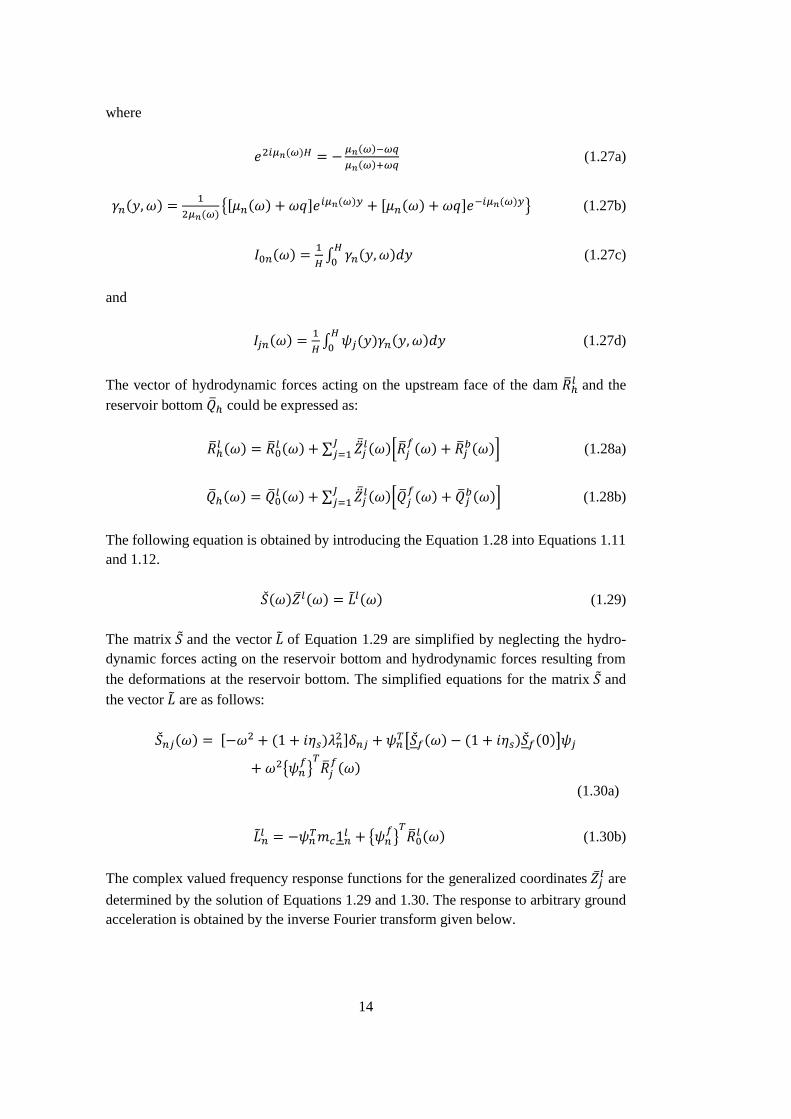
The vector of hydrodynamic forces acting on the upstream face of the dam and the
reservoir bottom could be expressed as:
∑ [
]
(1.28a)
∑
[
] (1.28b)
The following equation is obtained by introducing the Equation 1.28 into Equations 1.11
and 1.12.
(1.29)
The matrix and the vector of Equation 1.29 are simplified by neglecting the hydro-
dynamic forces acting on the reservoir bottom and hydrodynamic forces resulting from
the deformations at the reservoir bottom. The simplified equations for the matrix and
the vector are as follows:
[ ]
[ ]
{ }
(1.30a)
{
}
(1.30b)
The complex valued frequency response functions for the generalized coordinates are
determined by the solution of Equations 1.29 and 1.30. The response to arbitrary ground
acceleration is obtained by the inverse Fourier transform given below.
Page 31
15
∫
(1.31)
It should be noted that the generalized coordinates are factored with the Fourier trans-
formed ground acceleration . The displacement response in time domain is deter-
mined by the following equation.
∑ [
] (1.32)
The stresses in a finite element of the dam body is obtained by Equation 1.33 where
is the stresses at finite element p, is the displacements of the corresponding finite
element and is stress-transformation matrix of the element.
(1.33)
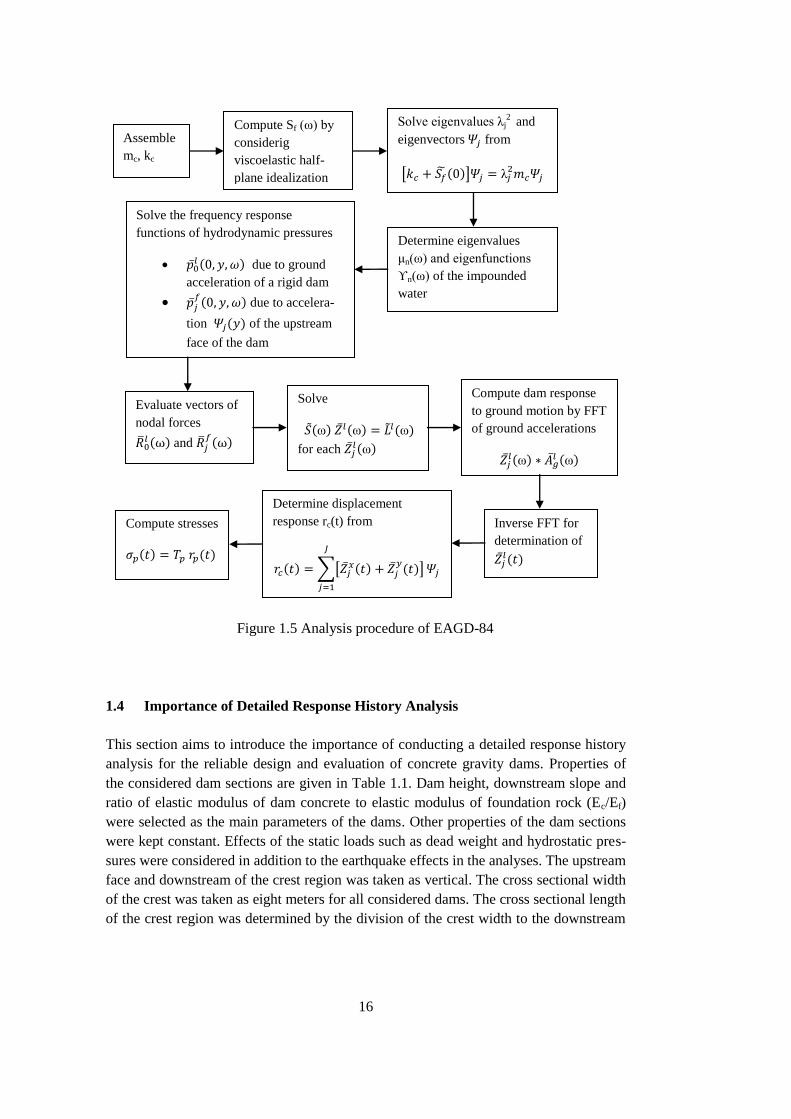
The general analytical procedure implemented by EAGD-84 is summarized as a
flowchart in Figure 1.5.
Page 32
16
1.4 Importance of Detailed Response History Analysis
This section aims to introduce the importance of conducting a detailed response history
analysis for the reliable design and evaluation of concrete gravity dams. Properties of
the considered dam sections are given in Table 1.1. Dam height, downstream slope and
ratio of elastic modulus of dam concrete to elastic modulus of foundation rock (Ec/Ef)
were selected as the main parameters of the dams. Other properties of the dam sections
were kept constant. Effects of the static loads such as dead weight and hydrostatic pres-
sures were considered in addition to the earthquake effects in the analyses. The upstream
face and downstream of the crest region was taken as vertical. The cross sectional width
of the crest was taken as eight meters for all considered dams. The cross sectional length
of the crest region was determined by the division of the crest width to the downstream
Assemble
mc, kc
Compute Sf (ω) by
considerig
viscoelastic half-
plane idealization [ ]
Solve eigenvalues j2 and
eigenvectors from
Determine eigenvalues
μn(ω) and eigenfunctions
ϒn(ω) of the impounded
water
Solve the frequency response
functions of hydrodynamic pressures
due to ground
acceleration of a rigid dam
due to accelera-
tion of the upstream
face of the dam
Evaluate vectors of
nodal forces
and
Solve
ω ω ω
for each ω
Inverse FFT for
determination of
∑[
]
Determine displacement
response rc(t) from Compute stresses
ω
ω
Compute dam response
to ground motion by FFT
of ground accelerations
Figure 1.5 Analysis procedure of EAGD-84
Page 33
17
slope of the dam. The optimum downstream slopes were computed for these dam sec-
tions by using two different approaches and results were critically evaluated.
First, the assessment method in BK guidelines was utilized for the determination of op-
timum downstream slopes by using response history analysis. For each section analyzed,
the smallest downstream slope was found such that dam stresses remain below the limits
as defined per BK guidelines. This slope is called the optimum downstream slope from
response history analysis (Table 1.1). This approach, named as the response history
analysis utilized the ground motion given in Chapter 3.
In order to demonstrate the importance of dynamic analysis, same dam sections were
reanalyzed by using the CADAM program and the optimum downstream slopes of the
dam cross sections were computed. The procedure of CADAM can be outlined as fol-
lows: First the spectrum of the ground motion was obtained for an equivalent damping
considering the dam-foundation-reservoir interaction. Secondly, the spectral accelera-
tion value at the fundamental frequency of the dam was computed and hydrodynamic
and inertial forces were determined. By using these forces, dam base stresses were
found by using the standard beam formulas. The principal tensile stress at the thalweg of
the dam was checked to see if the dam toe was overstressed. A dynamic amplification
factor of 1.50 was employed for the tensile strength of dam concrete. If the obtained
principal tensile stress at the thalweg was smaller than the factored tensile strength of
dam concrete (2.25 MPa for this case) the analyzed dam cross section could be accepted
as sufficient. The smallest downstream slope, which provided an acceptable principal
stress at the thalweg was referred as the optimum downstream slope from pseudo-static
analysis (Table 1.1).
Page 34
18
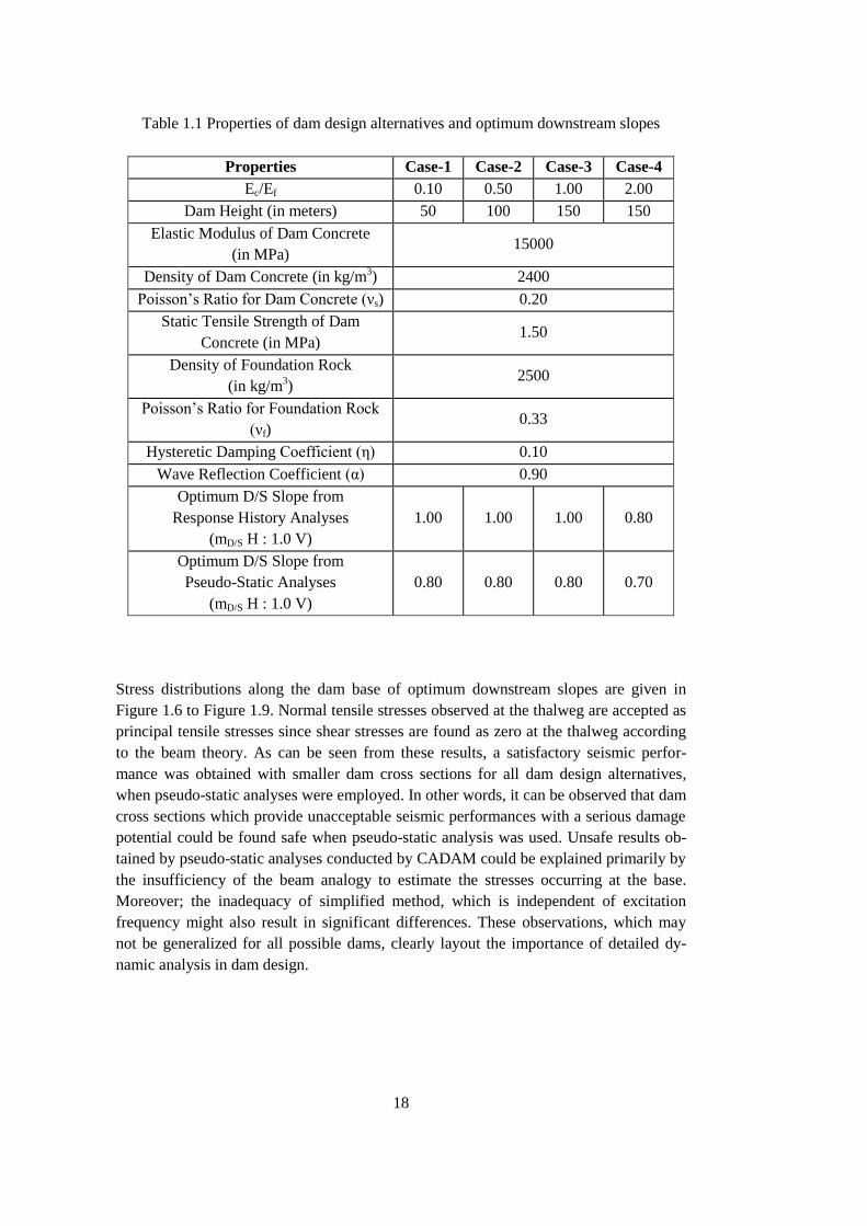
Table 1.1 Properties of dam design alternatives and optimum downstream slopes
Properties Case-1 Case-2 Case-3 Case-4
Ec/Ef 0.10 0.50 1.00 2.00
Dam Height (in meters) 50 100 150 150
Elastic Modulus of Dam Concrete
(in MPa) 15000
Density of Dam Concrete (in kg/m3) 2400
Poisson’s Ratio for Dam Concrete (νs) 0.20
Static Tensile Strength of Dam
Concrete (in MPa) 1.50
Density of Foundation Rock
(in kg/m3)
2500
Poisson’s Ratio for Foundation Rock
(νf) 0.33
Hysteretic Damping Coefficient (η) 0.10
Wave Reflection Coefficient (α) 0.90
Optimum D/S Slope from
Response History Analyses
(mD/S H : 1.0 V)
1.00 1.00 1.00 0.80
Optimum D/S Slope from
Pseudo-Static Analyses
(mD/S H : 1.0 V)
0.80 0.80 0.80 0.70
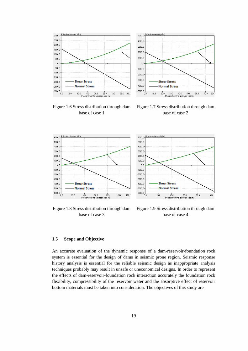
Stress distributions along the dam base of optimum downstream slopes are given in
Figure 1.6 to Figure 1.9. Normal tensile stresses observed at the thalweg are accepted as
principal tensile stresses since shear stresses are found as zero at the thalweg according
to the beam theory. As can be seen from these results, a satisfactory seismic perfor-
mance was obtained with smaller dam cross sections for all dam design alternatives,
when pseudo-static analyses were employed. In other words, it can be observed that dam
cross sections which provide unacceptable seismic performances with a serious damage
potential could be found safe when pseudo-static analysis was used. Unsafe results ob-
tained by pseudo-static analyses conducted by CADAM could be explained primarily by
the insufficiency of the beam analogy to estimate the stresses occurring at the base.
Moreover; the inadequacy of simplified method, which is independent of excitation
frequency might also result in significant differences. These observations, which may
not be generalized for all possible dams, clearly layout the importance of detailed dy-
namic analysis in dam design.
Page 35
19
Figure 1.6 Stress distribution through dam
base of case 1
Figure 1.7 Stress distribution through dam
base of case 2
Figure 1.8 Stress distribution through dam
base of case 3
Figure 1.9 Stress distribution through dam
base of case 4
1.5 Scope and Objective
An accurate evaluation of the dynamic response of a dam-reservoir-foundation rock
system is essential for the design of dams in seismic prone region. Seismic response
history analysis is essential for the reliable seismic design as inappropriate analysis
techniques probably may result in unsafe or uneconomical designs. In order to represent
the effects of dam-reservoir-foundation rock interaction accurately the foundation rock
flexibility, compressibility of the reservoir water and the absorptive effect of reservoir
bottom materials must be taken into consideration. The objectives of this study are
Page 36
20
To develop a user friendly graphical user interface to conduct seismic response
history analysis of concrete gravity dams.
To conduct parametric studies to understand effects of parameters on the seis-
mic response.
To investigate the most influential parameter by conducting a deterministic sen-
sitivity analysis with tornado diagrams approach.
To assess the structural performance of gravity dams with a probabilistic ap-
proach and determine fragility curves of a set of dams with various properties.
The determination of fragility curves aims to provide a reference for both pre-
liminary design of new dams and investigation of the structural reliability exist-
ing dams.
The development of the user interface is presented in Chapter 2. In Chapter 3 details of
conducted parametric studies, deterministic sensitivity analysis and the determination of
the fragility curves are discussed. The main conclusions of the conducted study are
summarized and suggestions for future studies are introduced in Chapter 4.
Page 37
21
CHAPTER 2
2 A USER INTERFACE FOR DAM ANALYSIS
In this chapter, the development of a user friendly interface for the analysis of earth-
quake response of concrete gravity dams is presented. Input parameters, pre-processing,
post-processing details and results for seismic safety check are discussed. A dam analy-
sis example is also provided for a better understanding of the capabilities of the devel-
oped interface.
2.1 General
Many of the design engineers in Turkey, unfortunately, use outdated procedures and
assumptions, such as rigid foundation, rigid dam body, incompressible water etc. even
for the final design of the dams. These assumptions were mainly inherited from the for-
mer approaches of earth fill dam design about four decades ago. However, the use of
such outdated analysis tools may result in uneconomical designs in some cases and may
result in unsafe designs for some others as demonstrated in Chapter 1. In this context,
the interface tool developed in this study aims to open a window for the use of modern
analysis procedures in dam design and assessment in Turkey by considering dam-
reservoir-foundation rock interactions appropriately. This chapter aims to explain the
key features of the developed interface along with an analysis example. The analysis
engine employed in this work is based on EAGD-84 with some modifications. Although
EAGD-84 is a comprehensive and widely accepted tool for seismic analysis of concrete
dams within the research community, it did not find much use in practice in Turkey due
to the difficulty of use. The product of this chapter is believed to overcome this limita-
tion of EAGD-84 and introduce it to the engineering community interested in dam de-
sign and safety assessment. The execution of the interface is conducted through -m func-
tions in Matlab. The developed Matlab scripts are compiled and converted to an execut-
able stand-alone program to allow functioning in Matlab absent environments. The use
of the interface is almost self explanatory, however key elements are described in this
chapter. The interface is designed to interact with the user by pop-up notification win-
dows in order to prevent entering improper data and other possible execution problems.
It should be noted that the accuracy of the results obtained by the program is directly
related with the quality and accuracy of the input data entered. Hence, it is the user’s
responsibility to judge the accuracy of the results.
Page 38
22
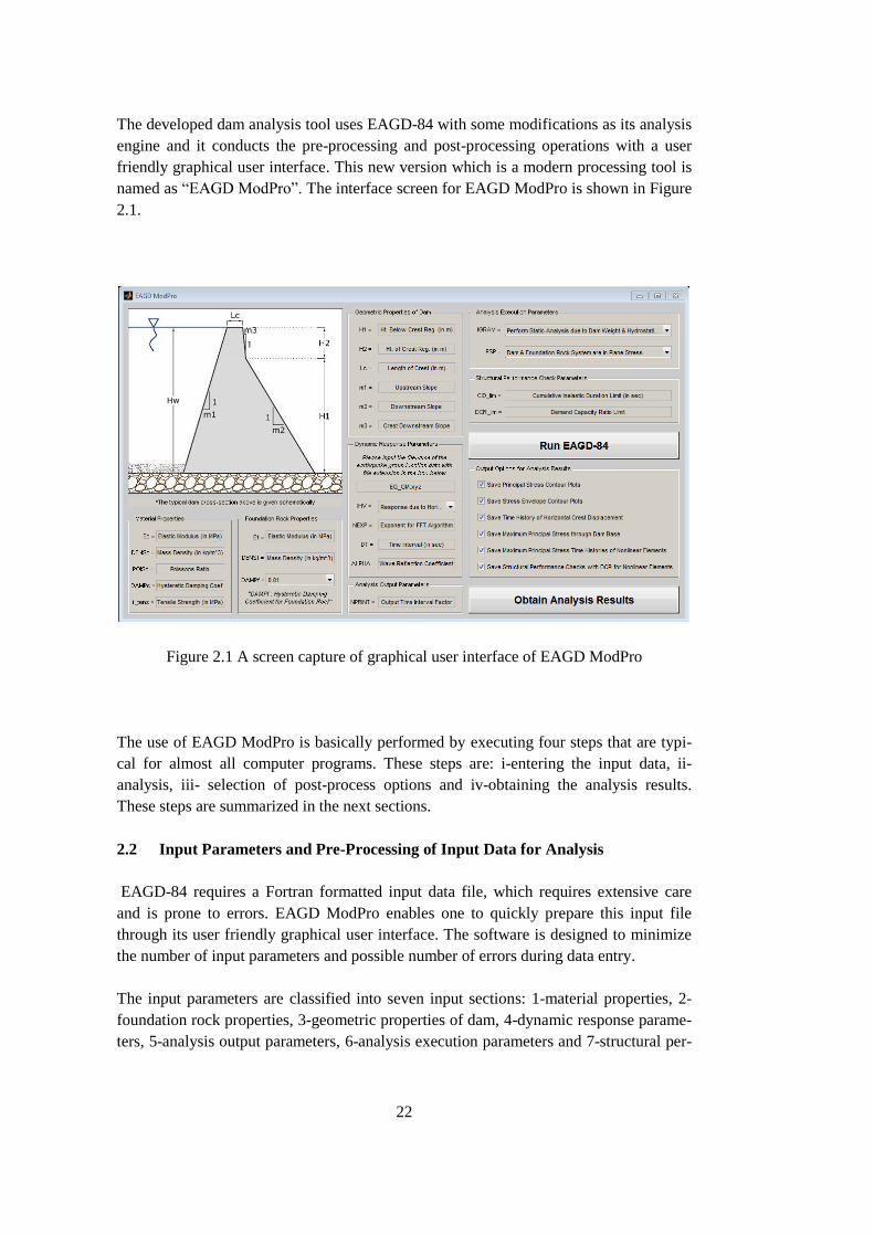
The developed dam analysis tool uses EAGD-84 with some modifications as its analysis
engine and it conducts the pre-processing and post-processing operations with a user
friendly graphical user interface. This new version which is a modern processing tool is
named as “EAGD ModPro”. The interface screen for EAGD ModPro is shown in Figure
2.1.
Figure 2.1 A screen capture of graphical user interface of EAGD ModPro
The use of EAGD ModPro is basically performed by executing four steps that are typi-
cal for almost all computer programs. These steps are: i-entering the input data, ii-
analysis, iii- selection of post-process options and iv-obtaining the analysis results.
These steps are summarized in the next sections.
2.2 Input Parameters and Pre-Processing of Input Data for Analysis
EAGD-84 requires a Fortran formatted input data file, which requires extensive care
and is prone to errors. EAGD ModPro enables one to quickly prepare this input file
through its user friendly graphical user interface. The software is designed to minimize
the number of input parameters and possible number of errors during data entry.
The input parameters are classified into seven input sections: 1-material properties, 2-
foundation rock properties, 3-geometric properties of dam, 4-dynamic response parame-
ters, 5-analysis output parameters, 6-analysis execution parameters and 7-structural per-
Page 39
23
formance parameters. It should be noted that EAGD-84, in its original form works in
imperial unit system. EAGD ModPro is prepared to work with metric system units. Fol-
lowing sections brief the data for each input section.
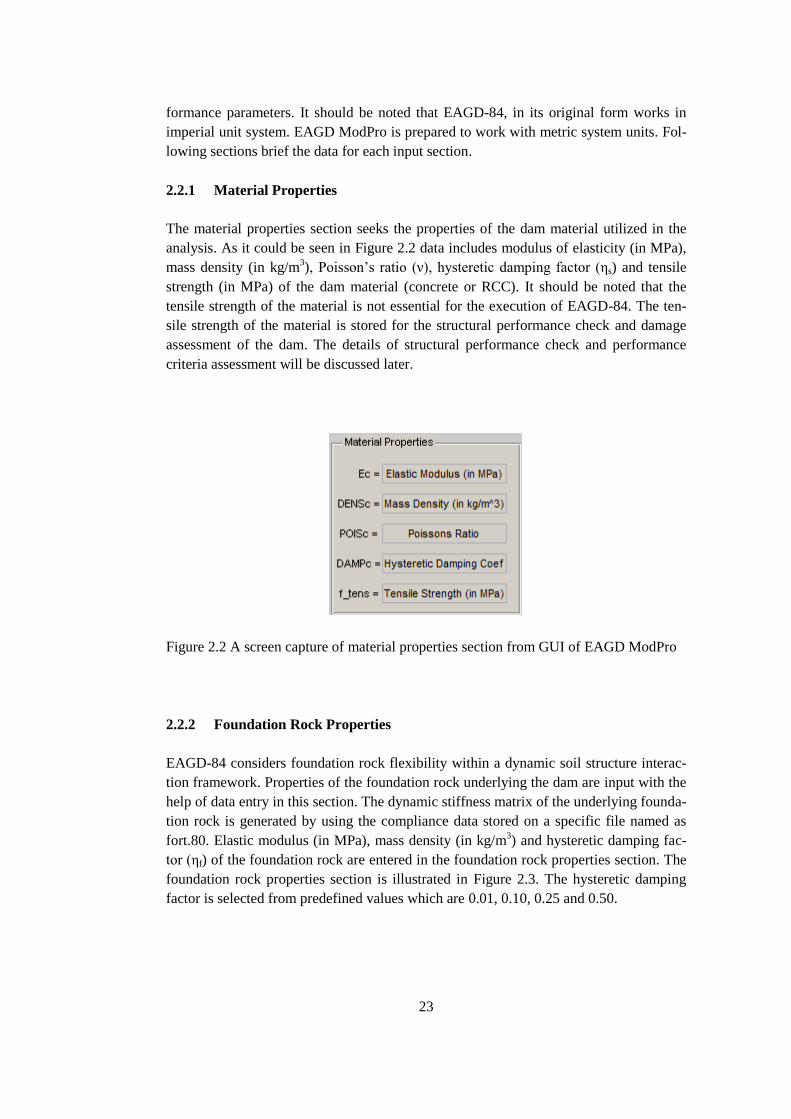
2.2.1 Material Properties
The material properties section seeks the properties of the dam material utilized in the
analysis. As it could be seen in Figure 2.2 data includes modulus of elasticity (in MPa),
mass density (in kg/m3), Poisson’s ratio (ν), hysteretic damping factor (ηs) and tensile
strength (in MPa) of the dam material (concrete or RCC). It should be noted that the
tensile strength of the material is not essential for the execution of EAGD-84. The ten-
sile strength of the material is stored for the structural performance check and damage
assessment of the dam. The details of structural performance check and performance
criteria assessment will be discussed later.
Figure 2.2 A screen capture of material properties section from GUI of EAGD ModPro
2.2.2 Foundation Rock Properties
EAGD-84 considers foundation rock flexibility within a dynamic soil structure interac-
tion framework. Properties of the foundation rock underlying the dam are input with the
help of data entry in this section. The dynamic stiffness matrix of the underlying founda-
tion rock is generated by using the compliance data stored on a specific file named as
fort.80. Elastic modulus (in MPa), mass density (in kg/m3) and hysteretic damping fac-
tor (ηf) of the foundation rock are entered in the foundation rock properties section. The
foundation rock properties section is illustrated in Figure 2.3. The hysteretic damping
factor is selected from predefined values which are 0.01, 0.10, 0.25 and 0.50.
Page 40
24
Figure 2.3 A screen capture of foundation rock properties section from GUI of EAGD
ModPro
User must be aware that a functional fort.80 file must be provided for the execution of
EAGD ModPro. The development of a complicated subroutine for the creation of dy-
namic compliance data stored on fort.80 file is beyond the scope of EAGD ModPro.
Various tools developed by other researchers are available for the creation of fort.80 file
(Akpinar 2013, Dasgupta 1977, 2012). EAGD ModPro focuses on conducting the pre
and post processing operations in the most efficient and user friendly way as possible.
It should be reminded it is possible to conduct analysis for a rigid foundation with
EAGD ModPro by choosing a sufficiently large modulus of elasticity for rock founda-
tion. It is recommended to use the elastic modulus of foundation rock as 50 times larger
than the elastic modulus of the dam material to ensure that rigid foundation behavior is
ensured.
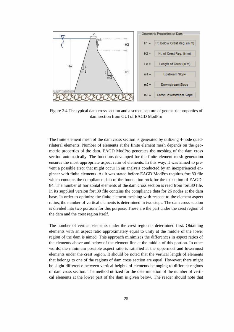
2.2.3 Geometric Properties of Dam
The geometric properties of dam section serves to create the geometry of the dam under
consideration. The user enters height below the crest (in meters), height of the crest (in
meters), length of the crest (in meters), upstream slope (horizontal:1), downstream slope
(horizontal:1) and downstream slope of crest region (horizontal:1). Full reservoir condi-
tion is taken into consideration. Therefore height of the water table is taken as the sum-
mation of height below crest region and height of crest region in the analysis. In graph-
ical user interface of EAGD ModPro a typical dam cross section demonstrating the input
parameters is given schematically in order to explain the input of the geometric proper-
ties of dam. The typical dam cross section and a screen capture of geometric properties
of dam section is given below (Figure 2.4).
Page 41
25
Figure 2.4 The typical dam cross section and a screen capture of geometric properties of
dam section from GUI of EAGD ModPro
The finite element mesh of the dam cross section is generated by utilizing 4-node quad-
rilateral elements. Number of elements at the finite element mesh depends on the geo-
metric properties of the dam. EAGD ModPro generates the meshing of the dam cross
section automatically. The functions developed for the finite element mesh generation
ensures the most appropriate aspect ratio of elements. In this way, it was aimed to pre-
vent a possible error that might occur in an analysis conducted by an inexperienced en-
gineer with finite elements. As it was stated before EAGD ModPro requires fort.80 file
which contains the compliance data of the foundation rock for the execution of EAGD-
84. The number of horizontal elements of the dam cross section is read from fort.80 file.
In its supplied version fort.80 file contains the compliance data for 26 nodes at the dam
base. In order to optimize the finite element meshing with respect to the element aspect
ratios, the number of vertical elements is determined in two steps. The dam cross section
is divided into two portions for this purpose. These are the part under the crest region of
the dam and the crest region itself.
The number of vertical elements under the crest region is determined first. Obtaining
elements with an aspect ratio approximately equal to unity at the middle of the lower
region of the dam is aimed. This approach minimizes the differences in aspect ratios of
the elements above and below of the element line at the middle of this portion. In other
words, the minimum possible aspect ratio is satisfied at the uppermost and lowermost
elements under the crest region. It should be noted that the vertical length of elements
that belongs to one of the regions of dam cross section are equal. However; there might
be slight difference between vertical heights of elements belonging to different regions
of dam cross section. The method utilized for the determination of the number of verti-
cal elements at the lower part of the dam is given below. The reader should note that
Page 42
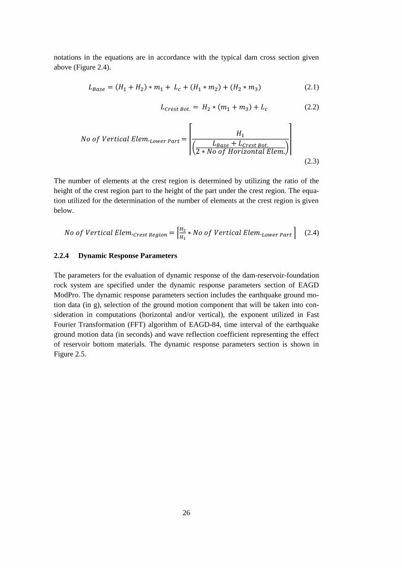
26
notations in the equations are in accordance with the typical dam cross section given
above (Figure 2.4).
(2.1)
(2.2)
⌈
(
)⌉
(2.3)
The number of elements at the crest region is determined by utilizing the ratio of the
height of the crest region part to the height of the part under the crest region. The equa-
tion utilized for the determination of the number of elements at the crest region is given
below.
⌈
⌉ (2.4)
2.2.4 Dynamic Response Parameters
The parameters for the evaluation of dynamic response of the dam-reservoir-foundation
rock system are specified under the dynamic response parameters section of EAGD
ModPro. The dynamic response parameters section includes the earthquake ground mo-
tion data (in g), selection of the ground motion component that will be taken into con-
sideration in computations (horizontal and/or vertical), the exponent utilized in Fast
Fourier Transformation (FFT) algorithm of EAGD-84, time interval of the earthquake
ground motion data (in seconds) and wave reflection coefficient representing the effect
of reservoir bottom materials. The dynamic response parameters section is shown in
Figure 2.5.
Page 43
27
Figure 2.5 A screen capture of dynamic response parameters section from GUI of
EAGD ModPro
The format of the earthquake ground motion data depends directly on the direction of
ground motion considered. If the dynamic response due to only horizontal or only verti-
cal component of the ground motion is computed the ground motion data must consist of
one column. If the dynamic response due to both horizontal and vertical components of
ground motion will be computed the ground motion data must consist of two columns in
one ground motion data file. The first column must include the horizontal component of
the ground motion data and the second column must include the vertical component of
the ground motion data. It should be noted that both columns must be the same in
length, thereby requiring zero padding for the shorter data. Time interval for both hori-
zontal and vertical components of the ground motion must also be same.
The selection of the time interval of earthquake ground motion data and the exponent
utilized in the FFT algorithm of EAGD-84 is directly related with the accuracy of the
analysis results. The other response parameters involved in the computation of the fre-
quency response functions and dynamic response of dam-reservoir-foundation rock
system with the use of the Fast Fourier Transform algorithm are selected in this selec-
tion. The equations for the determination of the other response parameters utilized in the
computations are summarized below. In these equations time interval of earthquake
ground motion and the exponent utilized in the Fast Fourier Transform algorithm are
denoted by DT and NEXP respectively.
Number of excitation frequencies /
Number of time intervals: (2.5)
Duration of response history: (2.6)
Page 44
28
Frequency increment:
(2.7)
Maximum frequency represented: (2.8)
The following conditions must be satisfied with the selection of the DT and NEXP val-
ues for the reliability of the analysis results (Fenves and Chopra, 1984):
i-The maximum excitation frequency must be greater than the frequencies of the consid-
erable harmonics resulting from the earthquake ground motion data. Therefore it is sug-
gested that the maximum excitation frequency must be greater than 25 Hz. In order to
satisfy this condition DT value must be selected less than or equal to 0.02 seconds.
EAGD ModPro enforces this condition while entering DT value with the help of a pop-
up notification window opened on the graphical user interface.
ii-The maximum vibration frequency must be greater than the frequency of the highest
vibration mode taken into account in the analysis. The analysis is conducted by consid-
ering ten generalized coordinates since the foundation rock flexibility is included. At the
end of each analysis EAGD ModPro prints the maximum excitation frequency and the
frequency of the highest vibration mode in a text file named as Natural Vibration Fre-
quencies.txt, which can be used to ensure the satisfaction of the above criterion.
iii-The number of excitation frequencies must be greater than the number of ground
accelerations read from the earthquake ground motion data. This condition must be ful-
filled by the selection of NEXP value. EAGD ModPro ensures the fulfillment of this
condition with the help of a pop-up notification window.
The frequency increment must be small enough to compute the frequency response
functions accurately. Moreover the aliasing error resulting from the FFT algorithm must
be minimized. In order to fulfill these requirements the maximum excitation frequency
must satisfy the following criterion. EAGD ModPro prints whether the criterion below
is satisfied or not into the text file stated above. One must also check the fulfillment of
the requirements with the help of this text file.
{
} (2.9)
EAGD ModPro utilizes compliance data stored in fort.80 file in order to determine the
dynamic stiffness matrix for the flexible foundation rock. The dynamic stiffness matrix
of the foundation rock is computed up to a certain maximum excitation frequency
(Equation 2.10). Therefore the maximum excitation frequency must be less than the
limit excitation frequency which the dynamic stiffness matrix is defined. The fulfillment
of this requirement depends on the satisfaction of the following criterion. EAGD Mod-
Pro secures meeting this criterion with the help of its graphical user interface.
Page 45
29
√ ⁄
(2.10)
It should be noted that Gf is the elastic shear modulus of the foundation rock (in k/ft2), f
is the density of the foundation rock (in k.sec2/ft
4) and b is the distance between the nod-
al points at the base of dam cross section (in ft) for the criterion stated above.
EAGD-84 considers the presence of reservoir-sediment interaction during the computa-
tion of the frequency response functions. The interaction between the sediment and res-
ervoir is taken into account by the wave reflection coefficient defined under dynamic
response parameters section. The reservoir bottom materials have an absorbing effect
due to a one dimensional damper like response during earthquake motions. The wave
reflection coefficient is simply as the ratio of the unabsorbed hydrodynamic pressure
waves reflected from the reservoir bottom. The wave reflection coefficient is recom-
mended as 0.9 to 1.0 for new dams, whereas it might be selected as 0.75 or 0.90 for the
analysis of older dams (Fenves and Chopra, 1986). It should be noted that usage of
higher values of wave reflection coefficient is a more conservative approach. Therefore;
in the case of the absence of reliable data, it is recommended to utilize higher values the
for wave reflection coefficient.
2.2.5 Analysis Output Parameters
The analysis output parameters section allows the selection of the time intervals to print
analysis results. The number of time intervals selected to print the analysis output has a
significant effect on the post-processing time of the raw analysis results. Moreover, the
size of raw output file depends on the number of time intervals. The previous experienc-
es show that printing the analysis output at every five time intervals is an appropriate
way for manageable data size. It should also be kept in mind that usage of too long time
intervals endanger the accuracy of the analysis outputs.
Figure 2.6 A screen capture of analysis output parameters section from GUI of EAGD
ModPro
Page 46
30
2.2.6 Analysis Execution Parameters
The analysis execution parameters section controls the type of the analyses i.e. whether
the effects of static loads such as dam weight and hydrostatic pressure are included and
the assumption made for two dimensional finite element analysis (plane stress or strain).
The dialogue box for this section is shown in Figure 2.7.
Figure 2.7 A screen capture of analysis execution parameters section from GUI of
EAGD ModPro
The effects of static loads on the dynamic response might be considered or ignored de-
pending on the user’s selection. The combination of the dynamic response with the re-
sponse due to static loads such as dam weight or hydrostatic pressure represents the
actual behavior of the dam-reservoir-foundation rock system. Printing only the dynamic
response option, on the other hand, gives the opportunity to investigate the absolute
effect of the strong ground motion on dam-reservoir-foundation rock system behavior.
The selection between plane stress and plane strain assumptions depends on the con-
struction methodology of the dam under investigation. If the keyed contraction joints (or
no transverse joints) are utilized during the construction, the monoliths of the dam may
be assumed to be behaving as a single unit under the strong ground motion. The use of
plane strain assumption is appropriate for this case. When the dam is designed with ver-
tical contraction joints, the monoliths of the dam may vibrate independently under the
strong ground motion. The plane stress assumption should be used for the representation
of dams designed with vertical contraction joints. It should be noted that plane stress and
plane strain assumptions are valid for gravity dams which are located in wide valleys.
Three dimensional analyses are required for gravity dams which are located in narrow
valleys and arch dams.
2.2.7 Structural Performance Check Parameters
EAGD ModPro is capable of performing the structural performance check and damage
criteria assessment of the dam analyzed according to BK Guidelines. The structural
Page 47
31
performance check parameters section stores the parameters necessary for the structural
performance check and damage assessment. The cumulative inelastic duration limit (in
seconds) and the demand capacity ratio limit for the elements experiencing nonlinear
behavior is entered in this section (Figure 2.8). The execution of EAGD-84 is independ-
ent from these parameters, even the raw analysis results data could be obtained without
entering any input at this section. However, it is essential to enter the parameters to op-
erate EAGD ModPro and to obtain the post-processed analysis results.
Figure 2.8 A screen capture of structural performance check parameters section from
GUI of EAGD ModPro
2.3 Analysis Results and Post-Processing of Raw Output Data
The procedure of the obtaining post-processed analysis results could be summarized by
the following four steps: i-the input variables, ii-execution of EAGD-84, iii-selection of
the appropriate output to be obtained after post-processing of raw analysis iv- execution
of EAGD ModPro to conduct post-processing operations. In EAGD ModPro the execu-
tion of EAGD-84 and the post-processing operations are conducted separately due to the
fact that post-processing operations consumes a considerable amount of time. In this
way it is intended to gain the opportunity of controlling the raw data results before con-
ducting lengthy post-processing operations. As it could be seen from Figure 2.9, the
execution of EAGD-84 and obtaining the post-processed analysis results are controlled
by different push buttons labeled as “Run EAGD-84” and “Obtain Analysis Results”.
Figure 2.9 Screen captures of the push buttons that control execution of EAGD-84 and
post-processing operations from GUI of EAGD ModPro
Page 48
32
The results that will be produced at the end of the execution of EAGD ModPro are se-
lected by the output options for analysis results section which could be seen in Figure
2.10. Since the output file obtained at the end of the analysis conducted by EAGD-84 is
impractical for the professional purposes, EAGD ModPro produces post-processed re-
sults which are user friendly and suitable for the professional purposes.
Figure 2.10 A screen capture of output options for analysis results section from GUI of
EAGD ModPro
EAGD ModPro produce contour plots for principal stresses and stress envelopes, time
history of horizontal crest displacement and maximum principal stress through dam
base. It should be noted that EAGD ModPro defines tensile stresses as positive. There-
fore; the term "maximum" for stress labels the highest tensile stress (or the smallest
compressive stress). In addition EAGD ModPro is also capable of conducting the struc-
tural performance check and damage criteria assessment of the dam analyzed according
to BK Guidelines.
The structural performance check and damage criteria assessment of the dam is con-
ducted in accordance with the methodology described in the design guideline published
by Concrete Dams Committee of DSİ (2012). The methodology described in the design
guideline is similar to the design and assessment approach recommended by US Army
Corps of Engineers (USACE, 2003). The sufficiency of the linear time history analysis
in deciding dam safety is conducted by EAGD ModPro by using this methodology. The
structural performance check and assessment of the damage is constituted on the de-
mand capacity ratio and cumulative inelastic stress duration terms. Demand capacity
ratio (DCR) represents the ratio of the tensile stress to the tensile strength of the con-
crete. In other words, nonlinear behavior is expected to initiate when the demand capaci-
ty ratio exceeds one. The cumulative duration of the stress levels above the tensile
Page 49
33
strength of concrete is taken as a measure of the damage estimation. As a damage indi-
cator the advantage of the cumulative inelastic stress duration over the classic number of
stress cycles approach is that it considers both magnitude and duration of the inelastic
stresses. For gravity dams, the acceptable limits for demand capacity ratio and cumula-
tive inelastic duration are 2 and 0.4 seconds respectively. As it is demonstrated in Figure
2.12, cumulative inelastic duration limit decreases linearly and reaches to zero when
demand capacity ratio is equal to 2. The validity of the assessment with linear time his-
tory analysis is determined by the cumulative inelastic duration curve for permitted de-
mand capacity ratio range (Figure 2.11). If the cumulative inelastic duration curve falls
below this performance limit curve, the expected performance of the dam is considered
as acceptable. Otherwise, nonlinear time history analysis is required for a more precise
damage assessment as the results from elastic analysis indicate the occurrence of visi-
ble/significant damage, which may or may not jeopardize dam safety. In addition to the
demand capacity ratio and cumulative inelastic duration limits, the cracked cross sec-
tional area should also be limited for the sufficiency of the assessment with linear time
history analysis. If the ratio of the cracked area to the cross section of the dam exceeds
15 percent nonlinear time history analysis is required (Ghanaat, 2004). This methodolo-
gy is implemented in EAGD ModPro for accurate and fast assessment of dam safety.
Figure 2.11 Computation of the
cumulative inelastic durations for
acceptable DCR levels
Figure 2.12 Structural performance check
and damage criteria assesment curve
-1.50
-1.00
-0.50
0.00
0.50
1.00
1.50
2.00
2.50
3.00
0 5 10 15
De
man
d C
apac
ity
Rat
io
Time (sec)
0
0.05
0.1
0.15
0.2
0.25
0.3
0.35
0.4
1 1.25 1.5 1.75 2Cu
mu
lati
ve In
ela
stic
Du
rati
on
(se
c)
Demand Capacity Ratio
Linear Assesment
is acceptable
Nonlinear assesment
is required
Page 50
34
2.4 A Dam Analysis Example Conducted with EAGD ModPro
The characteristics and capabilities of EAGD ModPro are discussed in detail in the pre-
vious sections. In order to better demonstrate the use of EAGD ModPro a dam analysis
example is presented in this section.
2.4.1 Modeling
The parameters for the dam material and foundation rock properties section are input as
shown in Figure 2.13 and Figure 2.14.
Figure 2.13 Input data entered under
material properties section
Figure 2.14 Input data entered under
foundation rock properties section
The geometric dimensions of the dam are input following the self explanatory notation
given in Figure 2.15. As it stated previously, the finite element mesh is generated auto-
matically by EAGD ModPro without needing any interaction with the user. The number
of finite elements used at the dam base is selected as 25 in this version and it depends on
the compliance data file (fort.80) utilized for the analysis.
Page 51
35
Figure 2.15 Input data entered under geometric properties of dam section and the typical
dam cross section
After the input of material properties and dam geometry, ground motion data is loaded
as shown in Figure 2.16. Only the horizontal component of the ground motion is taken
into consideration in this demonstration. As it is recommended for the case of the ab-
sence of reliable reservoir bottom information, the wave reflection coefficient is entered
as 0.9. The remaining dynamic response parameters are entered in accordance with the
limitations of EAGD-84 which are discussed previously. The data entered under dynam-
ic response parameters section is shown in Figure 2.17.
Figure 2.16 Horizontal earthquake ground
motion utilized for dam analysis example
Figure 2.17 Input data entered under
dynamic response parameters section
-0.4
-0.3
-0.2
-0.1
0
0.1
0.2
0.3
0 3 6 9 12 15
Ho
rizo
nta
l Gro
un
d M
oti
on
(g)
Time (sec)
Page 52
36
For this dam analysis example, the number of time intervals to print the analysis output
is selected as five to obtain an output file with a manageable data size (Figure 2.18). As
it could be seen from Figure 2.17 time interval of the earthquake ground motion data is
0.005 seconds; hence EAGD-84 will print the analysis result for every 0.025 seconds.
The selected number of time intervals to print the analysis output is recommended for
the acceptable time consumption during post processing operations.
Figure 2.18 Input data entered under analysis output parameters section
The effects of static loads such as dam weight and hydrostatic pressure are included in
the analysis results. The finite element analysis is conducted with the plane stress as-
sumption. The selected analysis execution options are shown in Figure 2.19.
Figure 2.19 Selected analysis execution options under analysis execution parameters
section
The dam analysis example includes the structural performance check and damage crite-
ria assessment of the dam. The structural performance check and damage assessment
parameters are selected in accordance with the recommendations for gravity dam as-
sessment (BK Guidelines, 2012). The cumulative inelastic duration limit is selected as
0.40 seconds and demand capacity ratio limit is selected as 2 (Figure 2.20). Tensile
strength of the dam concrete is taken as 1.5 MPa for this dam analysis example (Figure
2.13)
Page 53
37
Figure 2.20 Input data entered under structural performance check parameters section
Execution of EAGD ModPro is conducted by clicking the push button labeled as “Run
EAGD-84” (Figure 2.9). The post processed analysis results and outputs produced by
EAGD ModPro will be discussed in the following section.
2.4.2 Results
The raw data for the analysis results of the dam analysis example are stored in an output
file produced by the execution of EAGD ModPro, which post processes the results
stored on the output file and produces results which are in a suitable graphical format.
EAGD ModPro allows user to select the type of output for post processing operations.
In order to familiarize with the all output from EAGD ModPro, all the available output
options are selected for the dam analysis example (Figure 2.21).
Figure 2.21 Selected output options for the dam analysis example
EAGD ModPro produces outputs to give information about the utilized finite element
model for every conducted analysis. The details of the finite element model are printed
to a text file in order to better understand the numbering of the finite elements and ele-
Page 54
38
ment nodes. The text file which gives the details of the finite element meshing proper-
ties is shown at Figure 2.22. In addition to printing the details of the finite element
meshing properties in a text file, the finite element mesh and node/element numbering of
the dam cross section is also illustrated with as in Figure 2.23.
Figure 2.22 A screen capture from the text file which includes the detials of the finite
element meshing properties
Figure 2.23 The finete element meshing of the dam cross section
The natural vibration frequencies of the first ten vibration modes are printed for the dam
on an elastic foundation with empty reservoir case. As discussed in the dynamic re-
sponse parameters section, earthquake ground motion time interval (DT) and selected
exponent for the FFT algorithm (NEXP) must satisfy certain conditions in order to en-
Page 55
39
sure the accuracy of the dynamic analysis conducted. The verification of DT and NEXP
values are also included in the text file. The user must control the verification of DT and
NEXP values before utilizing the analysis results obtained from EAGD ModPro. The
text file which includes natural vibration frequencies and verification of DT and NEXP
values for the dam analysis example is shown in Figure 2.24.
Figure 2.24 A screen capture from the text file which includes natural vibration
frequencies and verificiation of selected NEXP and DT values
After post processing operations all the tiff files containing the finite element meshing,
contour plots, crest displacement history, maximum principal stress through dam base
and structural performance check plots are stored in a folder named as “Analysis Re-
sults” which is created in the same directory with EAGD ModPro. The maximum and
minimum principal stress contour plots produced by EAGD ModPro are shown in Fig-
ure 2.25 and Figure 2.26. In order to examine the stress level of elements easily, EAGD
ModPro plots the finite element meshing of the dam cross section on the contour plots.
In addition to principal stress contour plots, the contour plots which illustrate the axial
and shear stress envelopes of the elements are also produced (Figure 2.27 to Figure
2.32). All of the contour plots include color bars at the right hand side in order to
demonstrate the magnitude of the stress levels of elements.
Page 56
40
Figure 2.25 Maximum principal stress
contour plot
Figure 2.26 Minimum principal stress
contour plot
Figure 2.27 Maximum sigma-x envelope
contour plot
Figure 2.28 Minimum sigma-x envelope
contour plot
Figure 2.29 Maximum sigma-y envelope
contour plot
Figure 2.30 Minimum sigma-y envelope
contour plot
Page 57
41
Figure 2.31 Maximum thao-xy envelope
contour plot
Figure 2.32 Minimum thao-xy envelope
contour plot
In addition to the stress contour plots, time history of the horizontal crest displacement
and maximum principal stress through dam base are also produced and stored as image
files. Time history of the horizontal displacement displays the maximum upstream and
downstream displacements of the crest. The maximum principal stress envelope through
dam base provides information on the resulting stresses experienced at the dam founda-
tion. Time history of the horizontal crest displacement and maximum principal stress
through dam base are shown in Figure 2.33 and Figure 2.34.
Figure 2.33 Time history of horizontal
crest displacement
Figure 2.34 Maximum principal stress
through dam base
The structural performance check and damage criteria assessment is also conducted as a
part the dam analysis example. EAGD ModPro produces and stores the results of
structural performance check and damage assessment as tiff files. As a result of the
Page 58
42
structural performance check and damage assessment time history of the maximum
principal stress and cumulative inelastic duration curves are produced for each element
which experiences nonlinear behavior. Sufficiency of the assessment with linear time
history analysis is verified with these outputs. At the end of the dam analysis seven
elements exceeded the tensile strength of the concrete for the example under
consideration. The most critical damage generally appears at the thalweg region of the
dam, whose results are shown in Figure 2.35 and Figure 2.36.
Figure 2.35 Maximum principal stress
time history of the thalweg element
Figure 2.36 Cumulative inelastic
duration curve of the thalweg element
At the end of every analysis EAGD ModPro displays a massage window which shows
the ratio of the cracked cross sectional area to the dam cross section. For the sufficiency
of the structural performance check and damage criteria assessment user should also be
careful about whether the cracked area ratio exceeds the 15 percent limit or not. The
message window which is displayed at the end of the dam analysis example is given in
Figure 2.37.
Figure 2.37 Message window which shows the ratio of the cracked area to the dam cross
section
Page 59
43
CHAPTER 3
3 VULNERABILITY OF CONCRETE GRAVITY DAMS
Parametric studies performed to better understand the parameters affecting the seismic
response of concrete gravity dams are presented in this chapter. A deterministic sensitiv-
ity analysis was also conducted to display the most influential parameters. Afterwards,
fragility curves for gravity dams with typical sections were determined by using the
linear elastic procedures of seismic analysis and damage assessment.
3.1 Parametric Studies
This section presents the results of the analyses conducted to investigate the effects of
the material and dam geometry parameters on the performance of typical dam mono-
liths. In order to examine the effects of these parameters the optimum of the cross sec-
tions which provide an acceptable seismic performance is determined for dams with
various properties. The cross sectional area minimization which reduces the cost is con-
sidered as the objective of the optimization in this study. Therefor the cross section
which provides a satisfactory assessment result with the minimum cross sectional down-
stream slope is referred as the optimum dam cross section. For this purpose numerous
analyses were conducted for dams with various heights and properties. The conducted
analyses focus on the examination of effects of the variation of cross sectional down-
stream slope and ratio of elastic modulus of dam concrete to elastic modulus of founda-
tion rock (Ec/Ef).
A specific ratio of elastic modulus of dam concrete to elastic modulus of foundation
rock could be obtained by various values of elastic moduli of dam concrete and founda-
tion rock. Although all other parameters are kept same the selection of these values var-
ies the obtained principal stresses and performance curves (Figure 3.1). This variation is
resulting from the dominancy of the effect of variation of the elastic modulus of founda-
tion rock on the seismic analysis results (see Chapter 3.2). However; the utilization of
Ec/Ef ratio aims to investigate the effect of stiffening and softening of the foundation
rock on a specific dam case. For this purpose a specific value is selected for the elastic
modulus of dam concrete and elastic modulus of foundation rock values are determined
with the help of this value in the conducted analyses.
Page 60
44
a) Ec/Ef = 15000 MPa/7500 MPa
b) Ec/Ef = 10000 MPa/5000 MPa
Figure 3.1 Maximum principal stress contourplots and structural performance curves of
dams with the same Ec/Ef ratio (with different values of elastic moduli)
The parametric study was conducted for five dam heights with five cross sectional
downstream slope alternatives. Four ratios of elastic modulus of dam concrete to elastic
modulus of foundation rock were also included in the analyses. The values of dam
height, downstream slope and ratio of elastic modulus of dam concrete to elastic modu-
lus of foundation rock alternatives are shown in Table 3.1. In order to better distinguish
the effects of varying parameters on the seismic performance all other analysis parame-
ters are kept constant in the analyses. The constant values of the dam concrete and
foundation rock properties employed in the course of the analyses are given in Table
3.2. The wave reflection coefficient utilized in the analyses is selected as 0.9 as shown
in Table 3.2.
Page 61
45
Table 3.1 Values of the parameters utilized in parametric study
Parameters Values
Dam Height (in meters) 50, 75, 100, 125, 150
Downstream Slope (mD/S H : 1.0 V) 0.60, 0.70, 0.80, 0.90, 1.00
Ec/Ef 0.10, 0.50, 1.00, 2.00
Akkar (2010) conducted a site specific seismic hazard analysis for the Melen Dam loca-
tion and proposed a spectrum with a 2% probability of being exceeded in 50 years, i.e.
2475 years of return period (Figure 3.2). Then a synthetic ground motion was fitted to
the deaggregated spectrum (Figure 3.2). Only the horizontal component of the ground
motion data was proposed in that study.
Figure 3.2 Acceleration time history and acceleration response spectrum of the proposed
synthetic ground motion
-0.4
-0.3
-0.2
-0.1
0
0.1
0.2
0.3
0 3 6 9 12 15
Ho
rizo
nta
l Gro
un
d A
cce
lera
tio
n (
g)
Time (sec)
0
0.1
0.2
0.3
0.4
0.5
0.6
0.7
0.8
0.9
1
0 1 2 3 4
Spe
ctra
l Acc
ele
rati
on
(g)
Period (sec)
Page 62
46
Table 3.2 Values of the dam concrete properties and foundation rock properties utilized
in parametric study
Properties Values
Elastic Modulus of Dam Concrete (in MPa) 15000
Density of Dam Concrete (in kg/m3) 2400
Poisson’s Ratio for Dam Concrete (νs) 0.20
Static Tensile Strength of Dam Concrete (in MPa) 1.50
Density of Foundation Rock (in kg/m3) 2500
Poisson’s Ratio for Foundation Rock (νf) 0.33
Hysteretic Damping Coefficient (η) 0.10
Wave Reflection Coefficient (α) 0.90
The plane stress assumption is utilized for the conducted analyses. Influences of the
static loads such as dam weight and hydrostatic pressure are included in the analyses
results. The analyses are conducted with the full reservoir assumption which represents
the most critical situation. Foundation rock flexibility is taken into account with the
generated dynamic stiffness matrices for flexible foundation rock. The compliance data
which is stored in a file named as fort.80 is utilized for the determination of the dynamic
stiffness matrix of the flexible foundation. The same compliance data file is utilized for
all analyses. Since the foundation flexibility is taken into account, the analyses are con-
ducted by considering ten generalized coordinates (Fenves and Chopra, 1984).
The parametric study includes the analyses of numerous dams with different heights and
downstream slopes. The upstream faces of all dams are taken as vertical. The down-
stream of the crest region of all dams are also considered as vertical as well (Figure 3.3).
The cross sectional width of the dam crest is taken constant as eight meters for each
section. The cross section length of the crest region is determined by the division of the
crest width to the downstream slopes of dams. The finite element meshing of the dam
cross section is produced by 4-node quadrilateral finite elements. The number of finite
elements utilized for the meshing of the dam cross section is taken constant for all anal-
yses. The restriction of the number of finite elements aims to ease the comparison of the
analyses results of dams with different geometric properties and prevent possible dis-
crepancies resulting from inconsistent finite element meshing. The dam cross section is
divided into 25 elements in horizontal direction. In vertical direction dam section is di-
vided into a total of 25 elements. The crest region is divided into two elements and the
length below the crest region is divided into 23 elements. All of the dam alternatives are
analyzed with a finite element model with 625 elements. The typical finite element
meshing of the dam cross section is given in Figure 3.3.
Page 63
47
Figure 3.3 Typical dam meshing utilized in the parametric study
The accuracy of the stress distribution obtained with a finite element model containing
625 elements was verified by conducting analyses with different number of elements.
These analyses were conducted by considering static forces such as dead weight and
hydrostatic pressures and rigid foundation assumption. A typical dam section with a
height of 100 meters and a downstream slope of 0.80 was considered. All other analysis
parameters are taken same with the conducted parametric study. Finite element analyses
with 625 elements, 2500 elements and 5625 elements were conducted. Maximum prin-
cipal tensile stress distributions through the dam base obtained by using these finite
element models are compared (Figure 3.4). Although the obtained tensile stresses vary
for the first finite element at the thalweg, the stress distributions obtained by finite ele-
ment models with different number of elements are similar. It should be noted that mesh
refinement at a corner can always produce erroneous stresses. Hence checking the
stresses at some distance away from the corner provides some averaging and provides
more reliable stress estimations. Results indicate the stress error at the center of the first
base element for 625 elements has an error of about 19% compared to the stress at the
same location in the model with 5625 elements. This error is deemed as acceptable for
the purposes of this study.
Page 64
48
Figure 3.4 Maximum principal stresses through dam base obtained by different finite
element models
The area under the performance limit curve and the region of the structural performance
curve exceeding the performance limit curve (named hereafter as the Exceeded Area) is
computed for all dam alternatives of the parametric study. Computation of the Exceeded
Area is shown schematically in Figure 3.5. The magnitude of this area can be thought as
a measure of inelastic action expected. Analysis results for the exceeded area as a
function of downstream slope for different Ec/Ef ratios and dam heights are shown in
Figure 3.6.
Figure 3.5 Schematic illustration of the exceeded area
-0.250
0.250.5
0.751
1.251.5
1.752
2.252.5
0 20 40 60 80
Max
imu
m P
rin
cip
le S
tati
c St
ress
(in
MP
a)
Distance From Thalweg (in meters)
625 Elements2500 Elements5625 Elements
0
0.1
0.2
0.3
0.4
0.5
0.6
0.7
1 1.1 1.2 1.3 1.4 1.5 1.6 1.7 1.8 1.9 2
Cu
mu
lati
ve In
elas
tic
Du
rati
on
(s
ec)
Demand Capacity Ratio (for tension)
Exceeded Area (DCR.sec)
Page 65
49
a) Ec/Ef = 0.10
b) Ec/Ef = 0.50
c) Ec/Ef = 1.00
d) Ec/Ef = 2.00
Figure 3.6 The parametric study results for the thalweg elements of analyzed dams
The parametric study results clearly show that the increase of the ratio of elastic modu-
lus of dam concrete to elastic modulus of foundation rock decreases the stress levels of
the dam. The consideration of Ec/Ef results in more economical designs with smaller
downstream slopes. When the ratio of elastic modulus of dam concrete to elastic modu-
lus of foundation rock is 0.10 only the dam section which has 50 meters of height with a
downstream slope of 1.0 satisfies the design criterion. When the ratio of elastic modulus
of dam concrete to elastic modulus of foundation rock is increased to 0.50 the dam with
a height of 50 meters and a downstream slope of 0.90 appeared as the optimum cross
0
2
4
6
8
10
12
0.6 0.7 0.8 0.9 1
Exce
ed
ed
Are
a (D
CR
.se
c)
Downstream Slope
H = 50 m
H = 75 m
H = 100 m
H = 125 m
H = 150 m
0
1
2
3
4
5
6
7
8
9
10
0.6 0.7 0.8 0.9 1
Exce
ed
ed
Are
a (D
CR
.se
c)
Downstream Slope
H = 50 m
H = 75 m
H = 100 m
H = 125 m
H = 150 m
0
1
2
3
4
5
6
7
8
9
0.6 0.7 0.8 0.9 1
Exce
ed
ed
Are
a (D
CR
.se
c)
Downstream Slope
H = 50 m
H = 75 m
H = 100 m
H = 125 m
H = 150 m
0
0.5
1
1.5
2
2.5
3
3.5
4
0.6 0.7 0.8 0.9 1
Exce
ed
ed
Are
a (D
CR
.se
c)
Downstream Slope
H = 50 m
H = 75 m
H = 100 m
H = 125 m
H = 150 m
Page 66
50
section alternative. Dams with heights of 75 and 100 meters and the highest considered
downstream slope also exhibit acceptable seismic performance. When the ratio of elastic
modulus of dam concrete to elastic modulus of foundation rock is increased to 1.0 the
dams which have 50, 75 and 100 meters of height and a downstream slope of 0.90 satis-
fy the design criterion. Seismic performance of dams with heights of 125 and 150 and
the highest considered downstream slope are also satisfactory. When the ratio of elastic
modulus of dam concrete to elastic modulus of foundation rock is 2.0 the seismic per-
formance of all dams with a downstream slope of 0.80 are found as acceptable. These
observations underline the importance of taking the foundation rock flexibility into con-
sideration in the analyses. Softening of the foundation rock significantly decreases the
seismic stress demands which results in more economical designs. However when the
flexibility of the foundation rock is taken into account the bearing capacity of the foun-
dation rock must always be taken into consideration, which is excluded in this study.
The results of the parametric study show that the stress levels increase with the increase
of the dam height. This is an expected result since the hydrodynamic pressures and ef-
fects of the higher modes increases with the increase of dam height and reservoir depth.
The effects of the material and dam geometry parameters on the maximum horizontal
crest displacement (relative to the dam base) response which is an indicator of the seis-
mic performance are also investigated. Similar to the exceeded areas, the maximum
horizontal crest displacements are plotted as a function of downstream slope for differ-
ent Ec/Ef values (Figure 3.7). The results show that the maximum horizontal crest dis-
placements increase with the increase of the dam height. On the other hand as the cross
sectional downstream slope increases the obtained maximum horizontal crest displace-
ments decrease. The increase of the maximum crest displacement could be explained by
the increase of the slenderness of the dam cross section. Interestingly a significant varia-
tion of the maximum crest displacements could not be observed with the change of Ec/Ef
ratio. Although it might be expected that the total horizontal crest displacements in-
crease with the increase of the flexibility of foundation rock, relative horizontal crest
displacements with respect to the dam base are not affected by changes in Ec/Ef. It
should be reminded that these results may not be generalized for every possible ground
motion.
Page 67
51
a) Ec/Ef = 0.10
b) Ec/Ef = 0.50
c) Ec/Ef = 1.00
d) Ec/Ef = 2.00
Figure 3.7 Maximum horizontal crest displacements
It should be noted that all of these observations are valid only for gravity dams with
specific properties. Since the analyses are conducted with the plane stress assumption,
the parametric study results may not reflect the dams located in narrow valleys. Howev-
er; the conducted parametric study gives notable indications about the effects of parame-
ter selections on the behavior of the wide gravity dams.
0
0.05
0.1
0.15
0.2
0.25
0.6 0.7 0.8 0.9 1
Ho
rizo
nta
l Cre
st D
isp
lace
me
nt
(i
n m
ete
rs)
Downstream Slope
H = 50 mH = 75 mH = 100 mH = 125 mH = 150 m
0
0.05
0.1
0.15
0.2
0.25
0.6 0.7 0.8 0.9 1
Ho
rizo
nta
l Cre
st D
isp
lace
me
nt
(i
n m
ete
rs)
Downstream Slope
H = 50 mH = 75 mH = 100 mH = 125 mH = 150 m
0
0.05
0.1
0.15
0.2
0.25
0.6 0.7 0.8 0.9 1
Ho
rizo
nta
l Cre
st D
isp
lace
me
nt
(i
n m
ete
rs)
Downstream Slope
H = 50 mH = 75 mH = 100 mH = 125 mH = 150 m
0
0.05
0.1
0.15
0.2
0.25
0.6 0.7 0.8 0.9 1
Ho
rizo
nta
l Cre
st D
isp
lace
me
nt
(i
n m
ete
rs)
Downstream Slope
H = 50 mH = 75 mH = 100 mH = 125 mH = 150 m
Page 68
52
3.2 Deterministic Sensitivity Analysis (Tornado Diagrams)
Deterministic sensitivity analysis which is conducted for the investigation of the effects
of the random variables on the seismic response of a gravity dam is introduced in this
section. Tornado diagram method is utilized for the illustration of the effect of each
parameter independently. Tornado diagram arrays the investigated parameters with a
descending order in which the most influencing parameter at the top and the least influ-
encing one at the bottom. In order to obtain the tornado diagram, parameters to be con-
sidered are determined and several analyses are conducted by changing only one param-
eter at each case. When investigating the effect of a parameter a maximum and a mini-
mum value are considered as upper and lower boundaries. Other parameters are taken in
their median values in order to highlight the effect of the investigated parameter. The
difference of the results obtained for upper and lower boundaries of a parameter is de-
fined as swing. The length of swing indicates the effect of the random variable by
demonstrating the variability of the results. Tornado diagram is obtained by the ar-
rangement of the swings of each parameter in a descending order in which the largest
swing is located at the top. The production of the tornado diagram is shown in Figure
3.8.
Figure 3.8 Tornado diagram production process (Binici and Mosalam, 2007)
The influence of random variables are investigated by considering three engineering
demand parameters which are maximum principal tensile stress, maximum crest dis-
placement and the maximum value of the cumulative inelastic duration obtained by the
assessment with linear elastic analysis.
Page 69
53
The following parameters are selected as random variables to be investigated:
Elastic modulus of dam concrete (Ec)
Elastic modulus of foundation rock (Ef)
Hysteretic damping coefficient for dam concrete (ηc)
Hysteretic damping coefficient for foundation rock (ηf)
Ground motion data type (EQ Type)
Wave reflection coefficient (α)
Median, maximum and minimum values of the investigated parameters are given in
Table 3.3. The upper and lower boundaries and the variation of the parameters are se-
lected by considering a realistic representation of the extreme values appeared in real
life cases. A site specific seismic hazard analysis for the Melen Dam location was con-
ducted and a spectrum with a 2% probability of being exceeded in 50 years i.e. 2475
years of return period was proposed by Akkar in 2010. Three synthetic ground motions
which were fitted to the deaggregated spectrum were utilized as median, minimum and
maximum ground motions in the conducted deterministic sensitivity analysis. Only the
horizontal components of the ground motions are taken into consideration. Time histo-
ries and acceleration spectra of the ground motions are given in Figure 3.9.
Table 3.3 Input parameters utilized in deterministic sensitivity analysis
Parameters Median Minimum Maximum
Ec (in MPa) 20000 15000 25000
Ef (in MPa) 20000 5000 35000
ηc 0.10 0.05 0.15
ηf 0.10 0.01 0.25
α 0.90 0.80 1.00
Page 70
54
(a) Time history of the median ground
motion
(b) Time history of the minimum ground
motion
(c) Time history of the maximum ground
motion
(d) Acceleration response spectra of the
ground motions
Figure 3.9 Acceleration time histories and elastic response spectra of the proposed
synthetic ground motions
The other analysis parameters which affect the seismic response are kept constant in all
analyses. The properties of the dam concrete and foundation rock which are kept con-
stant during the analyses are given in Table 3.4. The assumptions utilized in analyses are
same with the assumptions made for the analyses conducted for parametric studies. The
plane stress assumption is utilized. Influences of the static loads are taken into account.
Full reservoir case is considered. Foundation rock flexibility is taken into consideration
with the same approach. Geometric idealizations and meshing properties of the finite
element model also identical with the ones employed in parametric studies.
-0.4
-0.3
-0.2
-0.1
0
0.1
0.2
0.3
0 10 20 30
Ho
rizo
nta
l Gro
un
d
Acc
ele
rati
on
(g)
Time (sec)
-0.4
-0.3
-0.2
-0.1
0
0.1
0.2
0.3
0.4
0 10 20
Ho
rizo
nta
l Gro
un
d
Acc
ele
rati
on
(g)
Time (sec)
-0.4
-0.3
-0.2
-0.1
0
0.1
0.2
0.3
0 5 10 15
Ho
rizo
nta
l Gro
un
d
Acc
eler
atio
n (
g)
Time (sec)
-0.1
0.1
0.3
0.5
0.7
0.9
0 2 4
Spe
ctra
l Acc
ele
rati
on
(g)
Period (sec)
MAX
MED
MIN
Page 71
55
Table 3.4 Values of the dam concrete properties and foundation rock properties utilized
in deterministic sensitivity analysis
Properties Values
Dam Height (in meters) 100
Downstream Slope (mD/S H : 1.0 V) 1.00
Density of Dam Concrete (in kg/m3) 2400
Poisson’s Ratio for Dam Concrete (νs) 0.20
Static Tensile Strength of Dam Concrete (in MPa) 1.50
Density of Foundation Rock (in kg/m3) 2500
Poisson’s Ratio for Foundation Rock (νf) 0.33
The median results obtained from the analysis of the median model are given Table 3.5.
The engineering demand parameters obtained by the median model were utilized for the
normalization of the results of conducted analyses. The analysis results are normalized
to 1 by dividing to the median model results. The normalized analyses results indicate
the ratio of variation, which is defined as swing, by the change of control parameter. The
tornado diagrams were obtained by the arrangement of the calculated swings.
Table 3.5 Median model results for engineering demand parameters
Demand Parameters Median Results
Maximum Principal Tensile Stress (in MPa) 2.715
Maximum Crest Displacement (in meters) 0.0405
Maximum Cumulative Inelastic Duration (in sec) 0.225
The results for maximum principal tensile stresses, maximum crest displacements and
maximum cumulative inelastic durations are given in Table 3.6 to Table 3.8. As it could
be seen from the results the increase of the ratio of elastic modulus of dam concrete to
elastic modulus of foundation rock increases the observed tensile stresses and inelastic
durations. This observation is parallel to the results of the parametric studies. The in-
crease of damping and reservoir bottom absorptions eases the responses as it is ex-
pected.
Page 72
56
Table 3.6 Maximum principal tensile stress results (in MPa)
Parameters Minimum Stress
(in MPa)
Maximum Stress
(in MPa)
Elastic Modulus of Dam Concrete (Ec) 3.128 2.343
Elastic Modulus of Foundation Rock (Ef) 0.372 2.920
Hysteretic Damping Coefficient
for Dam Concrete (ηc) 2.874 2.562
Hysteretic Damping Coefficient
for Foundation Rock (ηf) 3.152 2.100
Ground Motion Data Type (EQ Type) 2.435 2.792
Wave Reflection Coefficient (α) 2.650 2.775
The increase of elastic modulus of foundation rock decreased the observed maximum
crest displacement. This could be explained by the decrease of rigid body motion as a
result of the stiffening of the foundation rock. The stiffening of the dam body decreased
the obtained maximum crest displacement as it is expected.
Table 3.7 Maximum crest displacement results (in meters)
Parameters
Minimum Crest
Displacement
(in meters)
Maximum Crest
Displacement
(in meters)
Elastic Modulus of Dam Concrete (Ec) 0.0547 0.0323
Elastic Modulus of Foundation Rock (Ef) 0.0479 0.0380
Hysteretic Damping Coefficient
for Dam Concrete (ηc) 0.0417 0.0393
Hysteretic Damping Coefficient
for Foundation Rock (ηf) 0.0433 0.0365
Ground Motion Data Type (EQ Type) 0.0375 0.0408
Wave Reflection Coefficient (α) 0.0400 0.0407
Page 73
57
Table 3.8 Maximum cumulative inelastic duration results (in sec)
Parameters
Minimum
Cumulative
Inelastic
Duration (in sec)
Maximum
Cumulative
Inelastic
Duration (in sec)
Elastic Modulus of Dam Concrete (Ec) 0.25 0.1
Elastic Modulus of Foundation Rock (Ef) 0 0.7
Hysteretic Damping Coefficient
for Dam Concrete (ηc) 0.25 0.175
Hysteretic Damping Coefficient
for Foundation Rock (ηf) 0.3 0.1
Ground Motion Data Type (EQ Type) 0.1875 0.225
Wave Reflection Coefficient (α) 0.175 0.25
Tornado diagrams obtained by the arrangement of the swings of random variables are
given in Figure 3.10 to Figure 3.12. The elastic modulus of foundation rock appears to
be the most influencing parameter for the maximum principal tensile stress and maxi-
mum cumulative inelastic duration. The second most influential parameter for these
responses is the hysteretic damping coefficient of the foundation. The minimum value
selected for the foundation rock damping is considerably low. Therefore such a signifi-
cant effect resulting from the lower bound of hysteretic foundation rock damping is
pronounceable. The selection of such a value is a result of the restrictions due to availa-
ble compliance data and EAGD-84. It is observed that the elastic moduli of dam con-
crete and foundation rock are most and second most important parameters that affect the
maximum crest displacement. Ground motion type, hysteretic damping of the dam con-
crete and reservoir bottom absorption ratio are found as the least influencing parameters.
The obtained tornado diagrams demonstrate that the foundation rock properties such as
elastic modulus of foundation rock and hysteretic damping coefficient of foundation
rock have a significant influence on the engineering demand parameters. Therefore an
extensive care is required for the accurate determination of these parameters. It high-
lights the importance of rigorous site investigations, surveys and in-situ testing which
are essential for the correct estimation of the geological and geotechnical properties of
the dam site.
Page 74
58
Figure 3.10 Tornado diagram for maximum principal tensile stress
Figure 3.11 Tornado diagram for maximum crest displacement
Figure 3.12 Tornado diagram for maximum cumulative inelastic duration
0 0.2 0.4 0.6 0.8 1 1.2
α
ηc
EQ Type
Ec
ηf
Ef
Maximum Principal Tensile Stress
0.7 0.8 0.9 1 1.1 1.2 1.3 1.4
α
EQ Type
ηc
ηf
Ef
Ec
Maximum Crest Displacement
0 0.5 1 1.5 2 2.5 3 3.5
EQ Type
α
ηc
Ec
ηf
Ef
Maximum Cumulative Inelastic Duration
Page 75
59
3.3 Fragility Curves
This section aims to assess the structural performance of the gravity dams with a proba-
bilistic approach. For this purpose fragility curves of various dam alternatives are de-
termined. Since it is intended to produce a reference for both the preliminary design
phase of the new dams and the investigation of the structural reliability of existing dams
a wide range of dam alternatives are assessed. It should be reminded that the term fragil-
ity in the context used herein refers to the possibility of having visible damage as a re-
sult of significantly exceeding the linear response limits. In other words, fragility is not
meant to denote a probability of collapse for the purposes of this study.
Fragility analysis aims to evaluate the structural performance in probabilistic terms.
Fragility could be summarized as the conditional probability of failure of the structure.
The probabilistic structural performance evaluation and damage assessment of a struc-
ture is conducted with the determination of the fragility curves. Fragility curves exhibit
the probability of the exceeding a structural limit state as a function of the engineering
demand parameter. In this study, the sufficiency of the linear time history analysis for
the structural performance check and damage criteria assessment is taken as the limit
state for the dam which is subjected to strong ground motion. The methodology present-
ed in the design guideline published by Concrete Dams Committee of DSİ (2012) is
taken as the basis for the damage criteria assessment. The details of the methodology
and the determination of the sufficiency of the linear time history analysis for the dam-
age assessment and structural performance check are discussed previously. The spectral
acceleration at the fundamental mode of the dam is the engineering demand parameter
of the determined fragility curves.
Determination of the seismic fragility curve of a dam section requires the consideration
of the performances under a set of ground motions. The necessity of the consideration of
a set of ground motions is a direct result of the probabilistic approach of fragility analy-
sis. Determination of the acceleration response spectra of the considered ground motions
is the first step of the determination of the fragility curves. The acceleration response
spectra of ground motions were obtained by a computer program named as Utility Soft-
ware for Data Processing developed by Akkar et al. (personal communication, 2011).
The fundamental period of the dam with the full reservoir case is determined next. For
this purpose the dam with a full reservoir was subjected to a unit impulse which has a
magnitude of 1 m/s2. Effects of the static loads were excluded in the analysis. Fast Fou-
rier transformation of the horizontal crest displacement history of the analyzed dam was
performed and displacement results were obtained in the angular frequency domain.
Obtained displacement results are in a discrete form, thereby crest acceleration response
in the angular frequency domains was obtained by Equation 3.1. The fundamental angu-
lar frequency of the dam was determined by the investigation of the frequency which
corresponds to the first peak of the acceleration response. The fundamental angular fre-
quency is transformed to fundamental period by Equation 3.2.
Page 76
60
(3.1)
(3.2)
In Equation 3.1 and Equation 3.2 angular frequency, period, displacement response and
acceleration response in frequency domain are represented by , T, and respective-
ly.
The spectral acceleration demands for the fundamental period of the dam with a full
reservoir were determined from the obtained acceleration response spectra of the earth-
quake set. Seismic fragility curve of a dam basically demonstrates the probabilities of
observing unacceptable damage for a scale of spectral acceleration demand. For this
purpose dynamic analyses of a dam under a set of scaled ground motions must be con-
ducted. Scaling of the ground motion aims to obtain a spectral acceleration value which
is equal to the spectral acceleration demand at the fundamental period of the dam with a
full reservoir. Since performance evaluation of the dam is conducted by linear elastic
analysis, the scaling of the ground motion could be achieved by simply scaling the re-
sponse analysis results of the dam. Therefore, dynamic analyses of the dam under the set
of considered ground motions were conducted only once and the principal stress time
histories were scaled for the specific spectral acceleration demand. The factor utilized
for the scaling of the response results was obtained by the division of the spectral accel-
eration demand to the spectral acceleration for the fundamental period of a dam with a
full reservoir. Fragility analysis was conducted for a scale of spectral accelerations
which starts with zero and ends with 3.0 g. Spectral acceleration demands were in-
creased with an increment of 0.1 g. The initial fragility curve of the dam was obtained
by conducting a set of assessments for all spectral acceleration demands and determin-
ing the probabilities of observing visible damage.
The initial fragility curve obtained for the considered scale of spectral acceleration de-
mands was in a scatter data form. In order to determine a smooth fragility curve which is
suitable to cover all possible spectral acceleration demand values an exponential func-
tion of spectral accelerations was fitted to determined fragility data. The selected expo-
nential function is:
(3.3)
where is the spectral acceleration demand and and are the constants for the regu-
lation of the form of fragility curve. The selection of an exponential function aims to
represent the nature of the seismic fragility behavior of the concrete gravity dams. In
order to minimize the error while fitting fragility curves to fragility data the least squares
method is utilized for the determination of the values of constants and . The proce-
dure of the determination of a fragility curve is summarized in Figure 3.13.
Page 77
61
Figure 3.13 The procedure of the determination of a fragility curve
Determine the acceleration
response spectra of the
considered ground motions
0
0.1
0.2
0.3
0.4
0.5
0.6
0.7
0.8
0 0.5 1 1.5 2 2.5 3
Sa
T
Analyze the dam which is
subjected to a unit impulse of
1m/s2 (The dam with a full
reservoir case is taken into account
and effects of static loads are
excluded.).
Obtain the horizontal crest
displacement response in the
angular frequency domain by
the fast Fourier transformation
of the calculated crest
displacement history.
Obtain the horizontal crest
acceleration response in the
angular frequency domain
by
Determine the fundamental
angular frequency from the
first peak and obtain the
fundemental period by
Determine spectral acceleration demands for the
fundamental period of the dam from the acceleration
response spectra of the considered ground motions.
0
0.1
0.2
0.3
0.4
0.5
0.6
0.7
0.8
0 0.5 1 1.5 2 2.5 3
Sa
S1
Sn
S2
T1
Conduct dynamic analyses of the dam
for the considered ground motions. Scale
the dynamic response results for each
spectral acceleration demand by utilizing
linear elastic property of the analyses.
Obtain a smooth fragility curve by fitting
function to the computed fragility
data. The constants and are obtained by the least
squares method.
0.00
0.10
0.20
0.30
0.40
0.50
0.60
0.70
0.80
0.90
1.00
0.00 0.10 0.20 0.30 0.40 0.50 0.60 0.70 0.80 0.90 1.00
Pro
bab
ility
of
Ob
serv
ing
Vis
ible
Dam
age
Spectral Acceleration Sa (g)
Conduct the assessments with the scaled
dynamic responses and determine the
probabilities of observing visible damage
for all spectral acceleration demands.
Page 78
62
The determination of a set of fragility curves aims to produce a general reference for
concrete gravity dams. For this reason fragility analyses were conducted for dams with
various parameters. Five dam heights and three cross sectional downstream slopes alter-
natives were taken into consideration. Three ratios of elastic modulus of dam concrete to
elastic modulus of foundation rock (Ec/Ef) and static tensile strength of dam concrete
(ftens) alternatives were included. In order to reflect the analysis with rigid foundation
rock assumption one of the ratios of elastic modulus of dam concrete to elastic modulus
of foundation rock was selected as 0.02. The purpose of production a general reference
for both the preliminary design phase and the investigation of the structural reliability is
taken as the basis for the selection of these parameters. The values of considered dam
height, downstream slope, ratio of elastic modulus of dam concrete to elastic modulus of
foundation rock and tensile strength of dam concrete alternatives are given in Table 3.9.
Table 3.9 Values of the parameters utilized in fragility analysis
Parameters Values
Dam Height (in meters) 50, 75, 100, 125, 150
Downstream Slope (mD/S H : 1.0 V) 0.70, 0.85, 1.00
Ec/Ef 0.02, 1.00, 2.00
ftens (in MPa) 1.00, 1.50, 2.00
All other analysis parameters were kept constant in all analyses and these parameters are
selected in accordance with the general properties of the existing gravity dams. Since the
ratio of the elastic modulus of dam concrete to elastic modulus of foundation rock is a
parameter in fragility analysis, the elastic modulus of foundation rock is computed from
the assigned ratio and the selected elastic modulus of dam concrete. The elastic modulus
of the dam concrete is kept constant at the conducted analyses. Same hysteretic damping
coefficient is selected for both dam concrete and foundation rock. The values of the
properties of dam concrete and foundation rock are given in Table 3.10. The wave re-
flection coefficient is selected as 0.9 as could be seen in Table 3.10.
Page 79
63
Table 3.10 Values of the dam concrete properties and foundation rock properties utilized
in fragility analysis
Properties Values
Elastic Modulus of Dam Concrete (in MPa) 20000
Density of Dam Concrete (in kg/m3) 2400
Poisson’s Ratio for Dam Concrete (νs) 0.20
Density of Foundation Rock (in kg/m3) 2500
Poisson’s Ratio for Foundation Rock (νf) 0.33
Hysteretic Damping Coefficient (η) 0.10
Wave Reflection Coefficient (α) 0.90
Fragility curves were determined by using two dimensional analyses conducted with
plane stress assumption suitable for dam monoliths. The effects of the static loads which
are dam weight and hydrostatic pressure were included. Full reservoir condition was
taken into consideration. The effect of the foundation rock flexibility was included by
the generation of dynamic stiffness matrix of flexible foundation. The dynamic stiffness
matrix of the flexible foundation was determined with the compliance data stored in
fort.80 file. The same compliance data was utilized for all analyses performed for the
fragility curves. As a result of the consideration of the foundation rock flexibility ten
generalized coordinates were taken into account at the conducted analyses (Fenves and
Chopra, 1984). The results of the analyses were printed for every five ground motion
time interval to conserve time and data space.
The cross sectional width of the crest region is kept constant as eight meters. Both the
upstream faces and the downstream of the crest region of all dams are considered as
vertical. The cross sectional lengths of the crest region is determined by the division of
the constant crest width to the cross sectional downstream slopes. All dam cross sections
are meshed with 4-node quadrilateral finite elements. The same number of finite ele-
ments is utilized for the meshing of the dam cross section in all analyses. The number of
finite elements is restricted to prevent potential discrepancies resulting from inconsistent
finite element meshing. Dam cross section is divided into 25 elements in both horizontal
and vertical direction. The crest region is divided into two elements and the length be-
low crest region is divided into 23 elements in vertical direction. A total of 625 elements
are utilized for the meshing of the dam cross section. Geometric and finite element
meshing properties of the dam cross sections are parallel with the properties of the sec-
tions utilized at the conducted parametric studies. Since the typical finite element mesh-
ing of dam cross section utilized for parametric study is already given in Figure 3.3 an-
other figure is not given in this section.
Page 80
64
A set of earthquakes which includes data of 20 ground motions was utilized for the de-
termination of the fragility curves of the dam alternatives. Since the number of earth-
quakes utilized in fragility analysis is greater than the previous studies only acceleration
response spectra of ground motions and general information about the earthquakes are
given (Figure 3.14, Table 3.11).
Table 3.11 General information about the ground motions utilized in fragility analysis
EQ No. Name Location Date Soil Type Magnitude PGA
1 Coalinga USA 1983 Granite 6.5 0.136
2 Marmara Turkey 1999 Rock 7.4 0.167
3 Coalinga USA 1983 Granite 6.5 0.172
4 Campano-Lucano Italy 1980 Rock 6.5 0.181
5 Imperial Valley USA 1979 Granite 6.5 0.186
6 Bucharest Romania 1977 Rock 6.4* 0.194
7 Campano-Lucano Italy 1980 Rock 6.5 0.216
8 Marmara Turkey 1999 Rock 7.4 0.227
9 Northridge USA 1994 Rock 6.7 0.233
10 Friuli Italy 1976 Rock 6.3 0.316
11 Campano-Lucano Italy 1980 Rock 6.5 0.323
12 Tabas Iran 1978 Rock 6.4* 0.338
13 Friuli Italy 1976 Rock 6.3 0.357
14 Tabas Iran 1978 Rock 6.4* 0.385
15 Marmara Turkey 1999 Rock 7.4 0.407
16 Loma Prieta USA 1989 Rock 7 0.435
17 Loma Prieta USA 1989 Rock 7 0.442
18 North P. Springs USA 1986 USGS (A) 6.2 0.492
19 North P. Springs USA 1986 USGS (A) 6.2 0.612
20 Morgan Hill USA 1984 Rock 6.1 0.711
Page 81
65
(a) Earthquakes 1-5
(b) Earthquakes 6-10
(c) Earthquakes 11-15
(d) Earthquakes 16-20
Figure 3.14 Acceleration response spectra of the ground motions utilized in fragility
analyses
Fragility curves were grouped by taking the sectional geometry properties into consider-
ation. A group of fragility curves includes the fragility curves of a dam with a specific
height and cross sectional downstream slope. There are nine curves at each group for
0
0.1
0.2
0.3
0.4
0.5
0.6
0.7
0.8
0 1 2 3
Spec
tral
Acc
eler
atio
n (
g)
Period (sec)
Coalinga (1)
Marmara (2)
Coalinga (3)
Campano-Lucano (4)
Imperial Valley (5)
Period Limits
0
0.2
0.4
0.6
0.8
1
1.2
0 1 2 3
Spec
tral
Acc
eler
atio
n (
g)
Period (sec)
Bucharest (6)
Campano-Lucano (7)
Marmara (8)
Northridge (9)
Friuli (10)
Period Limits
0
0.2
0.4
0.6
0.8
1
1.2
1.4
1.6
0 1 2 3
Spe
ctra
l Acc
ele
rati
on
(g)
Period (sec)
Campano-Lucano (11)
Tabas (12)
Friuli (13)
Tabas (14)
Marmara (15)
Period Limits
0
0.5
1
1.5
2
2.5
0 1 2 3
Spe
ctra
l Acc
ele
rati
on
(g)
Period (sec)
Loma Prieta (16)
Loma Prieta (17)
North P. Springs (18)
North P. Springs (19)
Morgan Hill (20)
Period Limits
Page 82
66
every ratio of elastic modulus of dam concrete to elastic modulus of foundation rock and
tensile strength of dam concrete alternatives. In order to prevent confusion fragility
curves of dams with similar ratio of elastic modulus of dam concrete to elastic modulus
of foundation rock were plotted by the same color and marked with the same type of
token. On the other hand fragility curves of dams with the same tensile strength of dam
concrete were plotted by utilizing the same line style. There are fifteen groups of fragili-
ty curves since five dam height and three cross sectional downstream slope alternatives
are included in fragility analysis. Fragility curves are given in Figure 3.15 to Figure
3.29.
Figure 3.15 Fragility curves of dams with a height of 50 meters and a downstream slope
of 0.70
Page 83
67
Figure 3.16 Fragility curves of dams with a height of 50 meters and a downstream slope
of 0.85
Figure 3.17 Fragility curves of dams with a height of 50 meters and a downstream slope
of 1.00
Page 84
68
Figure 3.18 Fragility curves of dams with a height of 75 meters and a downstream slope
of 0.70
Figure 3.19 Fragility curves of dams with a height of 75 meters and a downstream slope
of 0.85
Page 85
69
Figure 3.20 Fragility curves of dams with a height of 75 meters and a downstream slope
of 1.00
Figure 3.21 Fragility curves of dams with a height of 100 meters and a downstream
slope of 0.70
Page 86
70
Figure 3.22 Fragility curves of dams with a height of 100 meters and a downstream
slope of 0.85
Figure 3.23 Fragility curves of dams with a height of 100 meters and a downstream
slope of 1.00
Page 87
71
Figure 3.24 Fragility curves of dams with a height of 125 meters and a downstream
slope of 0.70
Figure 3.25 Fragility curves of dams with a height of 125 meters and a downstream
slope of 0.85
Page 88
72
Figure 3.26 Fragility curves of dams with a height of 125 meters and a downstream
slope of 1.00
Figure 3.27 Fragility curves of dams with a height of 150 meters and a downstream
slope of 0.70
Page 89
73
Figure 3.28 Fragility curves of dams with a height of 150 meters and a downstream
slope of 0.85
Figure 3.29 Fragility curves of dams with a height of 150 meters and a downstream
slope of 1.00
Page 90
74
The fragility curves illustrated above exhibit consistency with the observations from the
parametric study. The increase of the ratio of elastic modulus of dam concrete to elastic
modulus of foundation rock decreases the probability of a visible damage in dam body
for a given specific spectral acceleration demand. Hydrodynamic pressures and the ef-
fects of the higher vibration modes increase with the increase of dam height. For a spe-
cific spectral acceleration demand as the dam height increases the probability of observ-
ing unacceptable seismic performance increases. As expected the probability of observ-
ing of serious damage decreases with the increase of the tensile strength of dam con-
crete. The cross sectional downstream slope of dam also has a significant effect on the
probability of the observing a nonlinear behavior. The enlargement of dam cross section
obviously decreases the probability of observing a visible damage at the end of the
strong ground motion. It should be noted that these conclusions are made by considering
other variable parameters as constant.
Spectral acceleration demands for specific probabilities of the observing visible damage
are also presented. 50 percent and 90 percent probabilities of observing serious damage
are considered. Spectral acceleration demand values were determined by the iterative
solution of the exponential equations which are fitted to fragility data to obtain a smooth
fragility curve. Spectral acceleration curves were grouped by considering ratio of elastic
modulus of dam concrete to elastic modulus of foundation rock. Each group includes
nine curves for the design parameter which are the D/S slope and tensile strength of dam
concrete. Spectral acceleration demands were plotted against dam heights. Spectral ac-
celeration demands curves are given in Figure 3.30 to Figure 3.35.
Figure 3.30 Spectral acceleration demands for 50% probability of observing visible
damage (Ec/Ef = 0.02)
0
0.2
0.4
0.6
0.8
1
1.2
50 75 100 125 150
Spec
tral
Acc
eler
atio
n (
g)
Dam Height (in meters)
D/S Slope =0.70 & f_tens=1.00D/S Slope =0.70 & f_tens=1.50D/S Slope =0.70 & f_tens=2.00D/S Slope =0.85 & f_tens=1.00D/S Slope =0.85 & f_tens=1.50D/S Slope =0.85 & f_tens=2.00D/S Slope =1.00 & f_tens=1.00D/S Slope =1.00 & f_tens=1.50D/S Slope =1.00 & f_tens=2.00
Page 91
75
Figure 3.31 Spectral acceleration demands for 50% probability of observing visible
damage (Ec/Ef = 1.00)
Figure 3.32 Spectral acceleration demands for 50% probability of observing visible
damage (Ec/Ef = 2.00)
0
0.5
1
1.5
2
2.5
50 75 100 125 150
Spec
tral
Acc
eler
atio
n (
g)
Dam Height (in meters)
D/S Slope=0.70 & f_tens=1.00D/S Slope=0.70 & f_tens=1.50D/S Slope=0.70 & f_tens=2.00D/S Slope=0.85 & f_tens=1.00D/S Slope=0.85 & f_tens=1.50D/S Slope=0.85 & f_tens=2.00D/S Slope=1.00 & f_tens=1.00D/S Slope=1.00 & f_tens=1.50
0
0.5
1
1.5
2
2.5
3
3.5
50 75 100 125 150
Spec
tral
Acc
eler
atio
n (
g)
Dam Height (in meters)
D/S Slope=0.70 & f_tens=1.00D/S Slope=0.70 & f_tens=1.50D/S Slope=0.70 & f_tens=2.00D/S Slope=0.85 & f_tens=1.00D/S Slope=0.85 & f_tens=1.50D/S Slope=0.85 & f_tens=2.00D/S Slope=1.00 & f_tens=1.00D/S Slope=1.00 & f_tens=1.50
Page 92
76
Figure 3.33 Spectral acceleration demands for 90% probability of observing visible
damage (Ec/Ef = 0.02)
Figure 3.34 Spectral acceleration demands for 90% probability of observing visible
damage (Ec/Ef = 1.00)
0
0.2
0.4
0.6
0.8
1
1.2
1.4
50 75 100 125 150
Spec
tral
Acc
eler
atio
n (
g)
Dam Height (in meters)
D/S Slope =0.70 & f_tens=1.00D/S Slope =0.70 & f_tens=1.50D/S Slope =0.70 & f_tens=2.00D/S Slope =0.85 & f_tens=1.00D/S Slope =0.85 & f_tens=1.50D/S Slope =0.85 & f_tens=2.00D/S Slope =1.00 & f_tens=1.00D/S Slope =1.00 & f_tens=1.50D/S Slope =1.00 & f_tens=2.00
0
0.5
1
1.5
2
2.5
3
3.5
50 75 100 125 150
Spec
tral
Acc
eler
atio
n (
g)
Dam Height (in meters)
D/S Slope=0.70 & f_tens=1.00D/S Slope=0.70 & f_tens=1.50D/S Slope=0.70 & f_tens=2.00D/S Slope=0.85 & f_tens=1.00D/S Slope=0.85 & f_tens=1.50D/S Slope=0.85 & f_tens=2.00D/S Slope=1.00 & f_tens=1.00D/S Slope=1.00 & f_tens=1.50
Page 93
77
Figure 3.35 Spectral acceleration demands for 90% probability of observing visible
damage (Ec/Ef = 2.00)
Spectral acceleration demands for a specific probability of observing visible damage
varies with a pattern consistent with the discussions made for fragility curves. Spectral
acceleration demand increases with the increase of the ratio of elastic modulus of dam
concrete to elastic modulus of foundation rock. A lower spectral acceleration demand is
required for the same probability of observing a serious damage as the dam height in-
creases. The increase of tensile strength of dam concrete and cross sectional downstream
slope results in the requirement of a higher spectral acceleration demand. However, an
exact conclusion could not be made for whether tensile strength of dam concrete or
cross sectional downstream slope is more effective. Spectral acceleration demand for the
dam with same properties increases with the increase of the probability of occurrence
nonlinear damage as it is expected. Some spectral acceleration demands which are not
consistent with the general fashion of the curves are also obtained. These demands could
be explained imperfections of the fitted exponential function.
Dam sections with a high risk of observing serious damage for a spectral acceleration
demand of 1.0 g can be summarized as follows. Almost all dam sections are under the
risk of unsatisfactory seismic performance when the ratio of elastic modulus of dam
concrete to elastic modulus of foundation rock is 0.02. When the ratio of elastic modulus
of dam concrete to elastic modulus of foundation rock is increased to 1.00, dam sections
with heights of 100 meters or higher and downstream slopes of 0.85 or smaller exhibits
a high risk of observing serious damage. When the ratio of elastic modulus of dam con-
crete to elastic modulus of foundation rock is increased to 2.00, only the dam sections
0
1
2
3
4
5
6
50 75 100 125 150
Spec
tral
Acc
eler
atio
n (
g)
Dam Height (in meters)
D/S Slope=0.70 & f_tens=1.00D/S Slope=0.70 & f_tens=1.50D/S Slope=0.70 & f_tens=2.00D/S Slope=0.85 & f_tens=1.00D/S Slope=0.85 & f_tens=1.50D/S Slope=0.85 & f_tens=2.00D/S Slope=1.00 & f_tens=1.00D/S Slope=1.00 & f_tens=1.50
Page 94
78
which have a downstream slope of less than 0.85 are under the risk of unacceptable
seismic performance.
The determination of the fragility data utilized for the fragility curves and obtained spec-
tral acceleration demand curves were conducted by plane stress assumption. Therefore
the obtained results are valid only for the dams which behave in accordance with the
plane stress assumption under a strong ground motion. In other words conducted anal-
yses do not give accurate estimations for gravity dams which are located in narrow val-
leys or arch dams. Moreover it should also be reminded that fragility curves are deter-
mined with analyses under several regulations. The determined fragility curves aims to
be utilized as a reference for the preliminary design phase of the new dams and the in-
vestigation of the structural reliability of existing dams. In order to obtain results with an
acceptable accuracy it is required to perform detailed analyses.
Page 95
79
CHAPTER 4
4 CONCLUSION
4.1 General
In this study, a user friendly interface for the dynamic analysis of concrete gravity dams
was presented and seismic response of concrete gravity dams was investigated. A com-
puter program named as EAGD-84 was utilized for the analyses conducted in this study.
EAGD-84 was employed as the analysis engine of the developed user interface.
Parametric studies were conducted to better understand the effects of parameters on the
seismic response of concrete gravity dams. The pseudo-static analyses of several dam
alternatives were conducted by utilizing a computer program named as CADAM. The
results of pseudo-static analyses were compared with the results of parametric studies to
underline the importance of the detailed response history analysis for the reliable design
of concrete gravity dams. A deterministic sensitivity analysis was conducted for the
determination of the most influential parameters. Moreover; the structural performance
of dams with typical sections and various properties was evaluated with a probabilistic
approach. Fragility curves of the dams were determined by assessments with linear elas-
tic analyses. The conclusions of these studies can be summarized as followings:
The stress levels are directly related with the ratio of elastic modulus of dam
concrete to elastic modulus of foundation rock. As the ratio increases the stress
level of the dam decreases. Therefore the consideration of foundation flexibility
might result in more economical designs with smaller downstream slopes. It
should be noted that the bearing capacity of the foundation rock must always be
taken into consideration when the foundation rock flexibility is taken into ac-
count.
The increase of the dam height results in increase at the stress level. The in-
crease of the stress levels could be explained by the increase of both hydrostatic
and hydrodynamic pressures and higher mode effects.
Elastic modulus of the foundation rock appears as the most influencing parame-
ter of the maximum principal tensile stress and the maximum cumulative inelas-
tic duration responses. On the other hand, the maximum crest displacement re-
sponse is mostly affected by the change of elastic modulus of dam concrete.
Page 96
80
The probability of observing visible damage is inversely proportional with the
tensile strength of concrete.
Increase of the cross sectional downstream slope decreases the probability of
unacceptable damage occurrence.
Investigations conducted by the plane stress and plane stress assumptions are
not valid for gravity dams located in narrow valleys or arch dams.
This study takes only the linear elastic behavior of dam-reservoir-foundation rock sys-
tem into consideration. The foundation rock was idealized as an isotropic, viscoelastic
half plane. The further studies might investigate the effect of nonlinear behavior on the
seismic response. The foundation rock idealization might also be improved by taking the
effect of layered foundations into consideration. A user friendly interface might be de-
veloped for the generation of compliance data for the flexible foundation. A study might
be conducted for the investigation of the reliability of gravity dams through the country.
Moreover; the shortcomings of two dimensional analyses might be investigated by uti-
lizing three dimensional results. Development of reliable procedures for the calibration
of two dimensional analyses results for the dams located in narrow valleys or arch dams
might also be practical for the professional purposes.
Page 97
81
5 REFERENCES
Akkar, S. (2010). Melen Barajı İçin Tasarım Spektrumunun Olasılık Hesaplarına
Dayalı Sismik Tehlike Analizi. Ankara: METU.
Arabshahi, H., & Lotfi, V. (2008). Earthquake Response of Concrete Gravity Dams
Including Dam-Foundation Interface Nonlinearities. Engineering Structures, Vol. 30,
3065-3073.
Bhattacharjee, S. S., & Leger, P. (1994). Application of NFLM Models to Predict
Cracking in Concrete Gravity Dams. Journal of Structural Engineering, Vol. 120, No. 4,
1255-1271.
Bhattacharjee, S. S., & Leger, P. (1995). Fracture Response of Gravity Dams due to
Rise of Reservoir Elevation. Journal of Structural Engineering, Vol. 121, No. 9, 1298-
1305.
Binici, B., & Mosalam, K. M. (2007). Analysis of Reinforced Concrete Columns
Retrofitted with Fiber Reinforced Polymer Lamina. Composites: Part B, Vol. 38, 265-
276.
BK. (2012). Beton Barajlar Tasarım İlkeleri Rehberi. 1. Barajlar Kongresi (Rehber:
004). Ankara: DSİ.
Bougacha, S., Tassoulas, J. L., & Roesset, J. M. (1993). Analysis of Foundations on
Fluid-Filled Poroelastic Stratum. Journal of Structural Engineering Mechanics, Vol.
119, No. 8, 1632-1648.
Bougacha, S., Tassoulas, J. L., & Roesset, J. M. (1993). Dynamic Stiffness of
Foundations on Fluid-Filled Poroelastic Stratum. Journal of Structural Engineering
Mechanics, Vol. 119, No. 8, 1649-1662.
Chopra, A. K. (1966). Hydrodynamic Pressures on Dams During Earthquakes.
Berkeley, California: Structures and Materials Research, 66-2.
Dagupta, G., & Chopra, A. K. (1977). Dynamic Stiffness Matrices for Homogenous
Viscoelastic Halfplanes. California, Berkeley: Earthquake Engineering Research Center,
UCB/EERC-77/26.
Fenves, G., & Chopra, A. K. (1984). EAGD-84 A Computer Program for Earthquake
Analysis of Concrete Gravity Dams. Berkeley, California: Earthquake Engineering
Research Center, UCB/EERC-84/11.
Fenves, G., & Chopra, A. K. (1984). Earthquake Analysis and Response of Concrete
Gravity Dams. Berkeley, California: Earthquake Engineering Research Center,
UCB/EERC-84/10.
Page 98
82
Fenves, G., & Chopra, A. K. (1986). Simplified Analysis for Earthquake Resistant
Design of Concrete Gravity Dams. Berkeley, California: Earthquake Engineering
Research Center, UCB/EERC-85/10.
Ghanaat, Y. (2004). Failure Modes Approach to Safety Evaluation of Dams. 13th World
Conference on Earthquake Engineering. Vancouver, B.C., Canada.
Javanmardi, F., Leger, P., & Tinawi, R. (2005). Seismic Structural Stability of Concrete
Gravity Dams Considering Transient Uplift Pressures in Cracks. Engineering
Structures, Vol. 27, 616-628.
Lotfi, V., Roesset, J. M., & Tassoulas, J. L. (1987). A Technique for the Analysis of the
Response of Dams to Earthquakes. Earthquake Engineering and Structural Dynamics,
Vol. 15, 463-490.
Medina, F., Dominguez, J., & Tassoulas, J. L. (1990). Response of Dams to Earthquakes
Including Effects of Sediments. Journal of Structural Engineering, Vol. 116, No. 11,
3108-3121.
Öziş, Ü., & Alsan, M. (1990, July). Beton Baraj İnşaatının Türkiye'de Gelişmesi. İMO
Teknik Dergi, pp. 147-158.
US Army Corps of Engineers. (2003). Time-History Dynamic Analysis of Concrete
Hydraulic Structures. Washington, DC: Engineering and Design, EP 1110-2-6051.
Westergaard, H. M. (1933). Water Pressures on Dams During Earthquakes. American
Society of Civil Engineers, 419-472.
World Energy Council Turkish National Committee. (2012). Enerji Raporu 2012.
Ankara.
Yakut, A., & Erduran, E. (2004). Drift Based Damage Functions for Reinforced
Concrete Columns. Computers and Structures, Vol. 82, 121-130.