Page 1
SEISMIC PROTECTION OF BRIDGE STRUCTURES USING
SHAPE MEMORY ALLOY-BASED ISOLATION SYSTEMS
AGAINST NEAR-FIELD EARTHQUAKES
A Dissertation
by
OSMAN ESER OZBULUT
Submitted to the Office of Graduate Studies of
Texas A&M University
in partial fulfillment of the requirements for the degree of
DOCTOR OF PHILOSOPHY
December 2010
Major Subject: Civil Engineering
Page 2
Seismic Protection of Bridge Structures Using Shape Memory Alloy-Based Isolation
Systems against Near-Field Earthquakes
Copyright 2010 Osman Eser Ozbulut
Page 3
SEISMIC PROTECTION OF BRIDGE STRUCTURES USING
SHAPE MEMORY ALLOY-BASED ISOLATION SYSTEMS
AGAINST NEAR-FIELD EARTHQUAKES
A Dissertation
by
OSMAN ESER OZBULUT
Submitted to the Office of Graduate Studies of
Texas A&M University
in partial fulfillment of the requirements for the degree of
DOCTOR OF PHILOSOPHY
Approved by:
Chair of Committee, Stefan Hurlebaus
Committee Members, Jose Roesset
Monique Head
Ibrahim Karaman
Head of Department, John Niedzwecki
December 2010
Major Subject: Civil Engineering
Page 4
iii
ABSTRACT
Seismic Protection of Bridge Structures Using Shape Memory Alloy-Based Isolation
Systems against Near-Field Earthquakes. (December 2010)
Osman Eser Ozbulut, B.S., Istanbul Technical University;
M.S., Texas A&M University
Chair of Advisory Committee: Dr. Stefan Hurlebaus
The damaging effects of strong ground motions on highway bridges have
revealed the limitations of conventional design methods and emphasized the need for
innovative design concepts. Although seismic isolation systems have been proven to be
an effective method of improving the response of bridges during earthquakes, the
performance of base-isolated structures during near-field earthquakes has been
questioned in recent years. Near-field earthquakes are characterized by long period and
large- velocity pulses. They amplify seismic response of the isolation system since the
period of these pulses usually coincides with the period of the isolated structures.
This study explores the feasibility and effectiveness of shape memory alloy
(SMA)-based isolation systems in order to mitigate the response of bridge structures
against near-field ground motions. SMAs have several unique properties that can be
exploited in seismic control applications. In this work, uniaxial tensile tests are
conducted first to evaluate the degree to which the behavior of SMAs is affected by
variations in loading rate and temperature. Then, a neuro-fuzzy model is developed to
Page 5
iv
simulate the superelastic behavior of SMAs. The model is capable of capturing rate- and
temperature-dependent material response while it remains simple enough to carry out
numerical simulations. Next, parametric studies are conducted to investigate the
effectiveness of two SMA-based isolation systems, namely superelastic-friction base
isolator (S-FBI) system and SMA/rubber-based (SRB) isolation system. The S-FBI
system combines superelastic SMAs with a flat steel-Teflon bearing, whereas the SRB
isolation system combines SMAs with a laminated rubber bearing rather than a sliding
bearing. Upon evaluating the optimum design parameters for both SMA-based isolation
systems, nonlinear time history analyses with energy balance assessment are conducted
to compare their performances. The results show that the S-FBI system has more
favorable properties than the SRB isolation system. Next, the performance of the S-FBI
systems is compared with that of traditional isolation systems used in practice. In
addition, the effect of outside temperature on the seismic response of the S-FBI system is
assessed. It is revealed that the S-FBI system can successfully reduce the response of
bridges against near-field earthquakes and has excellent re-centering ability.
Page 6
v
DEDICATION
To my loving mother,
who believed in and supported me in everything that I have ever wanted to do
Page 7
vi
ACKNOWLEDGEMENTS
I would like to thank my advisor, Dr. Stefan Hurlebaus for providing me the
opportunity to work with him and for his constant support and guidance throughout my
study. I would like to also thank my committee members, Dr. Jose Roesset, Dr.
Monique Head, and Dr. Ibrahim Karaman for their advice throughout the course of this
research. I am also grateful to Dr. Paul Roschke for his support and encouragement
since the beginning of my graduate study at Texas A&M University.
I also want to extend my gratitude to all of my friends for making me feel as at
home as possible during my time in Bryan/College Station. Finally, I would like to
thank my family for their infinite support, especially to my sisters, Sezen Kirtil and Esen
Ozbulut for their encouragement given to me to continue my education overseas.
Page 8
vii
TABLE OF CONTENTS
Page
ABSTRACT ..................................................................................................................... iii
DEDICATION ................................................................................................................... v
ACKNOWLEDGEMENTS .............................................................................................. vi
TABLE OF CONTENTS .................................................................................................vii
LIST OF FIGURES ........................................................................................................... xi
LIST OF TABLES ....................................................................................................... xviii
NOMENCLATURE ........................................................................................................ xix
1. INTRODUCTION ...................................................................................................... 1
1.1 Problem Description ......................................................................................... 1 1.2 Scope of Research ............................................................................................ 3 1.3 Organization of the Dissertation....................................................................... 5
2. SHAPE MEMORY ALLOYS: AN OVERVIEW ..................................................... 7
2.1 Introduction to Shape Memory Alloys ............................................................. 7 2.1.1 Shape Memory Effect ........................................................................ 9
2.1.2 Superelastic Effect ........................................................................... 11 2.1.3 Commonly-used Shape Memory Alloys ......................................... 13
2.1.3.1 NiTi-based alloys ....................................................... 13 2.1.3.2 Copper-based alloys ................................................... 14
2.1.3.3 Iron-based alloys ........................................................ 15 2.2 Mechanical Characteristics of Shape Memory Alloys ................................... 15
2.2.1 Characteristics of NiTi Alloy .......................................................... 16
2.2.1.1 Cycling loading .......................................................... 16
2.2.1.2 Strain rate effects ........................................................ 18
2.2.1.3 Temperature effects .................................................... 19
2.2.2 Characteristics of Cu-based Alloys ................................................. 20
2.2.2.1 Cycling loading .......................................................... 21
2.2.2.2 Strain rate effects ........................................................ 22
2.2.2.3 Temperature effects .................................................... 22
2.2.2.4 Grain size effects ........................................................ 23
Page 9
viii
Page
2.3 Modeling of Shape Memory Alloys ............................................................... 24
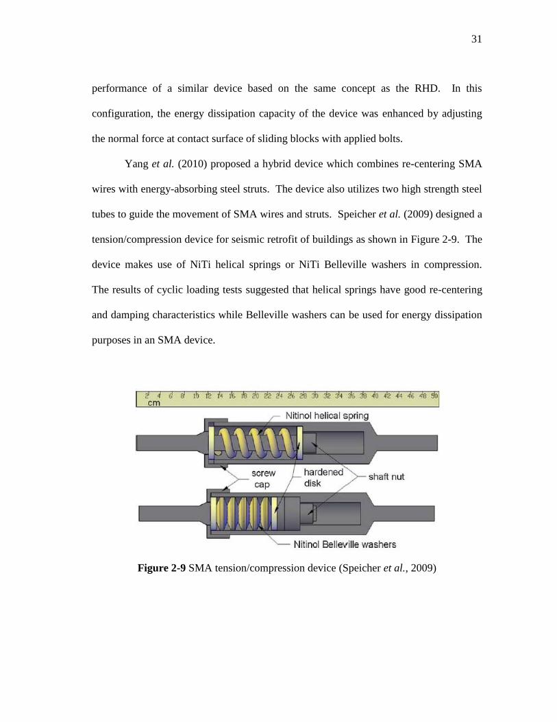
2.4 Seismic Applications of Shape Memory Alloys ............................................ 27 2.4.1 Applications to Buildings ................................................................ 27
2.4.1.1 SMA-based devices .................................................... 27
2.4.1.2 SMA bracing systems ................................................. 32
2.4.1.3 SMA beam-column connectors .................................. 34
2.4.1.4 SMA-based isolation devices ..................................... 36
2.4.2 Applications to Bridges ................................................................... 37
2.4.2.1 SMA restrainers .......................................................... 37
2.4.2.2 SMA dampers for cable-stayed bridges ..................... 39
2.4.2.3 SMA reinforcement .................................................... 41
2.4.2.4 SMA-based isolation devices ..................................... 43
3. EXPERIMENTAL TESTS ON SUPERELASTIC SMAs ....................................... 44
3.1 Introduction .................................................................................................... 44
3.2 Experimental Procedure ................................................................................. 44 3.2.1 Material and Specimen .................................................................... 44
3.2.2 Experimental Apparatus .................................................................. 45
3.2.3 Testing Procedure ............................................................................ 46
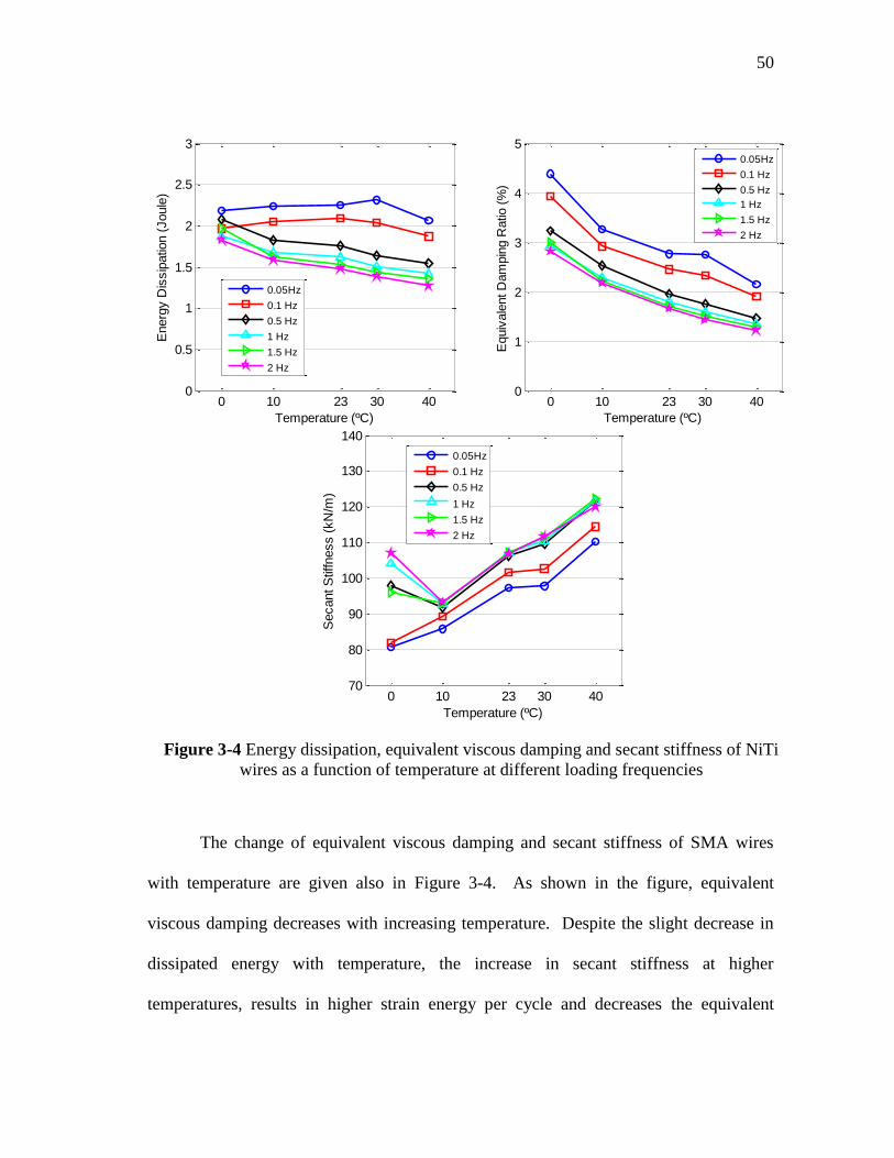
3.3 Experimental Results ...................................................................................... 47
3.3.1 Temperature Effects ........................................................................ 47
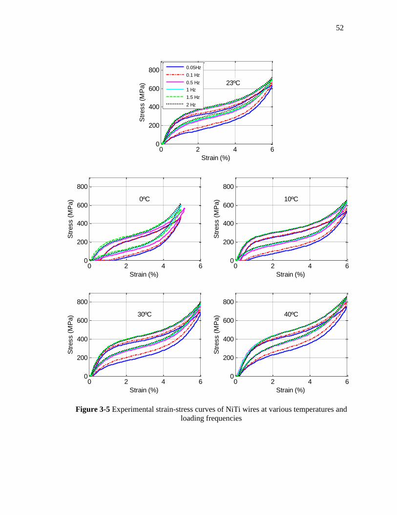
3.3.2 Strain Rate Effects ........................................................................... 51
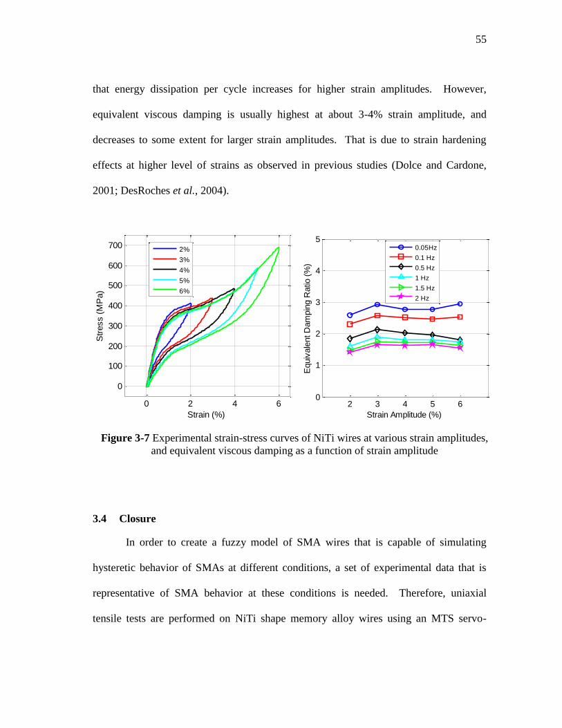
3.3.3 Strain Amplitude Effects ................................................................. 54
3.4 Closure ........................................................................................................... 55
4. NEURO-FUZZY MODELING OF TEMPERATURE- AND STRAIN-RATE-
DEPENDENT BEHAVIOR OF SMAs ................................................................... 57
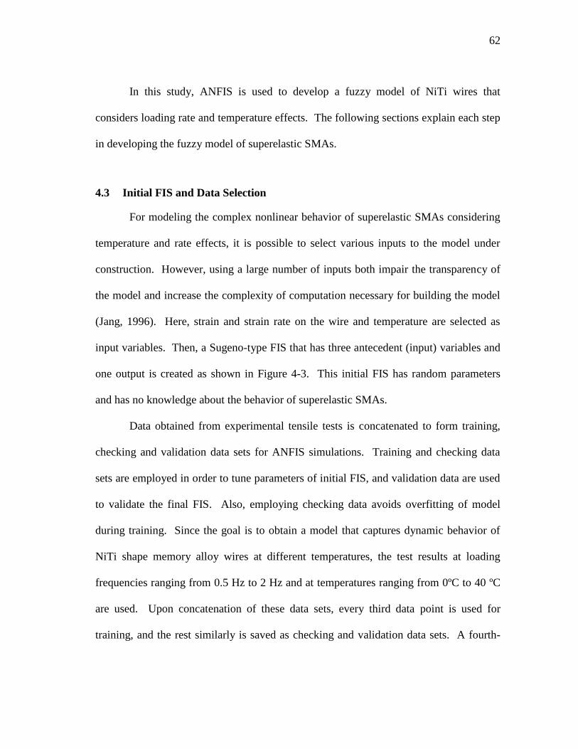
4.1 Introduction .................................................................................................... 57 4.2 Neuro-Fuzzy Modeling .................................................................................. 57 4.3 Initial FIS and Data Selection ........................................................................ 62
4.4 ANFIS Training .............................................................................................. 63 4.5 Model Validation ............................................................................................ 67 4.6 Closure ........................................................................................................... 67
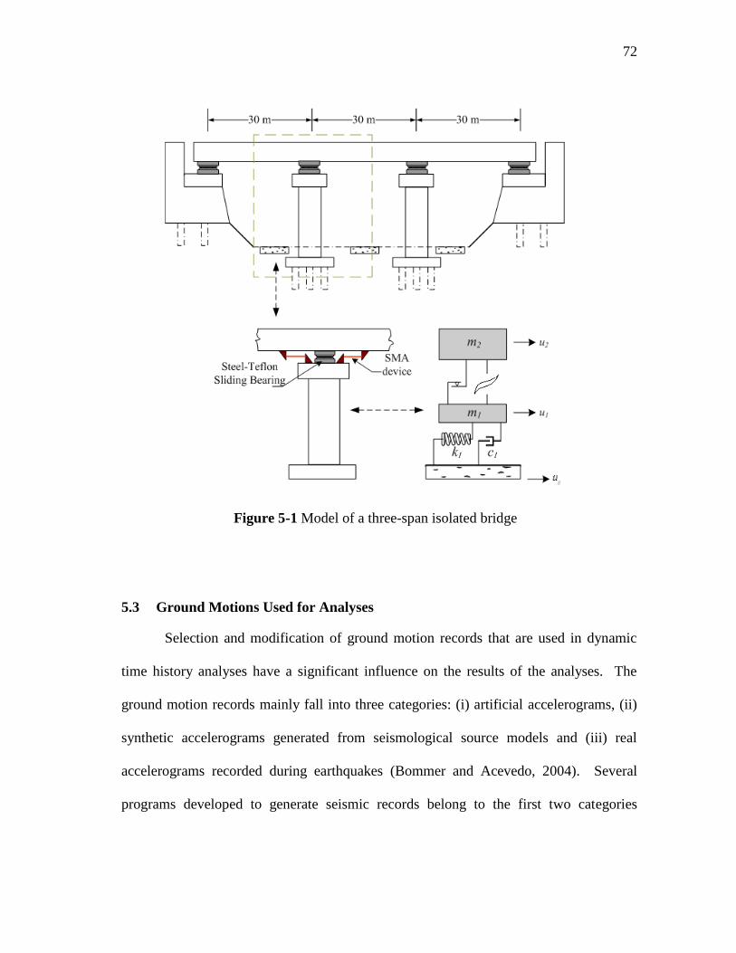
5. SUPERELASTIC-FRICTION BASE ISOLATORS ............................................... 69
5.1 Introduction .................................................................................................... 69
5.2 Model of Isolated Bridge Structure ................................................................ 70 5.3 Ground Motions Used for Analyses ............................................................... 72 5.4 Sensitivity Analysis ........................................................................................ 76
Page 10
ix
Page
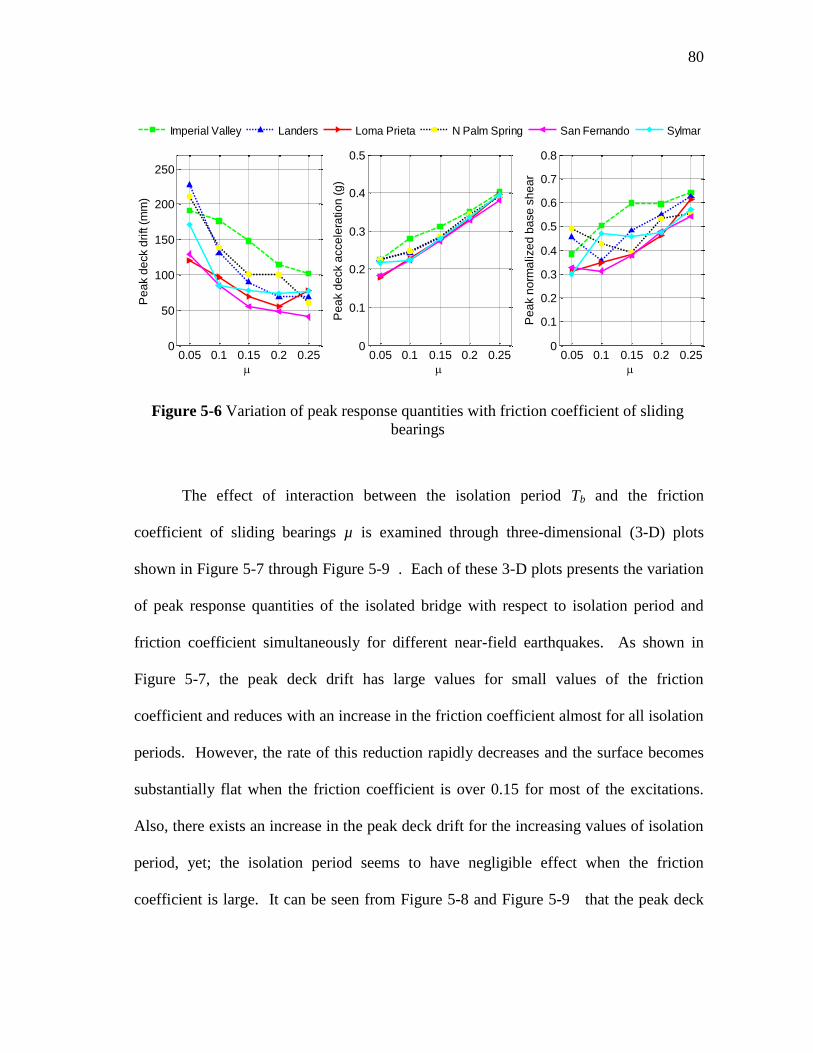
5.5 Results of Sensitivity Analysis ....................................................................... 78
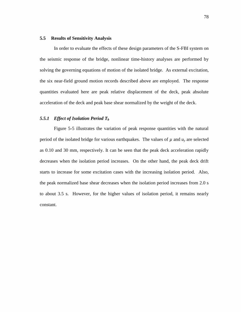
5.5.1 Effect of Isolation Period Tb ........................................................... 78
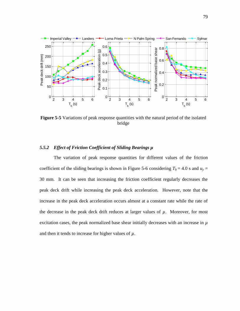
5.5.2 Effect of Friction Coefficient of Sliding Bearings µ ....................... 79
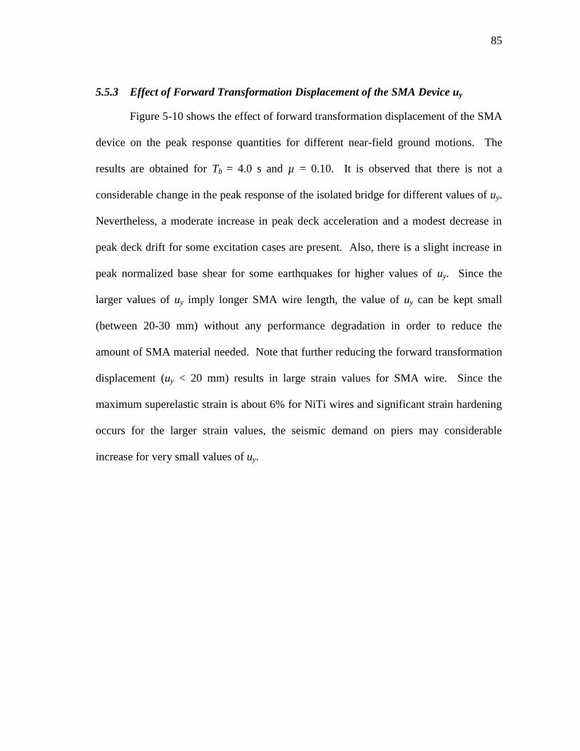
5.5.3 Effect of Forward Transformation Displacement of the SMA
Device uy ......................................................................................... 85
5.5.4 Effect of Ambient Temperature ...................................................... 86
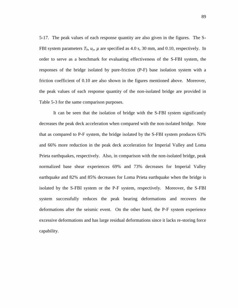
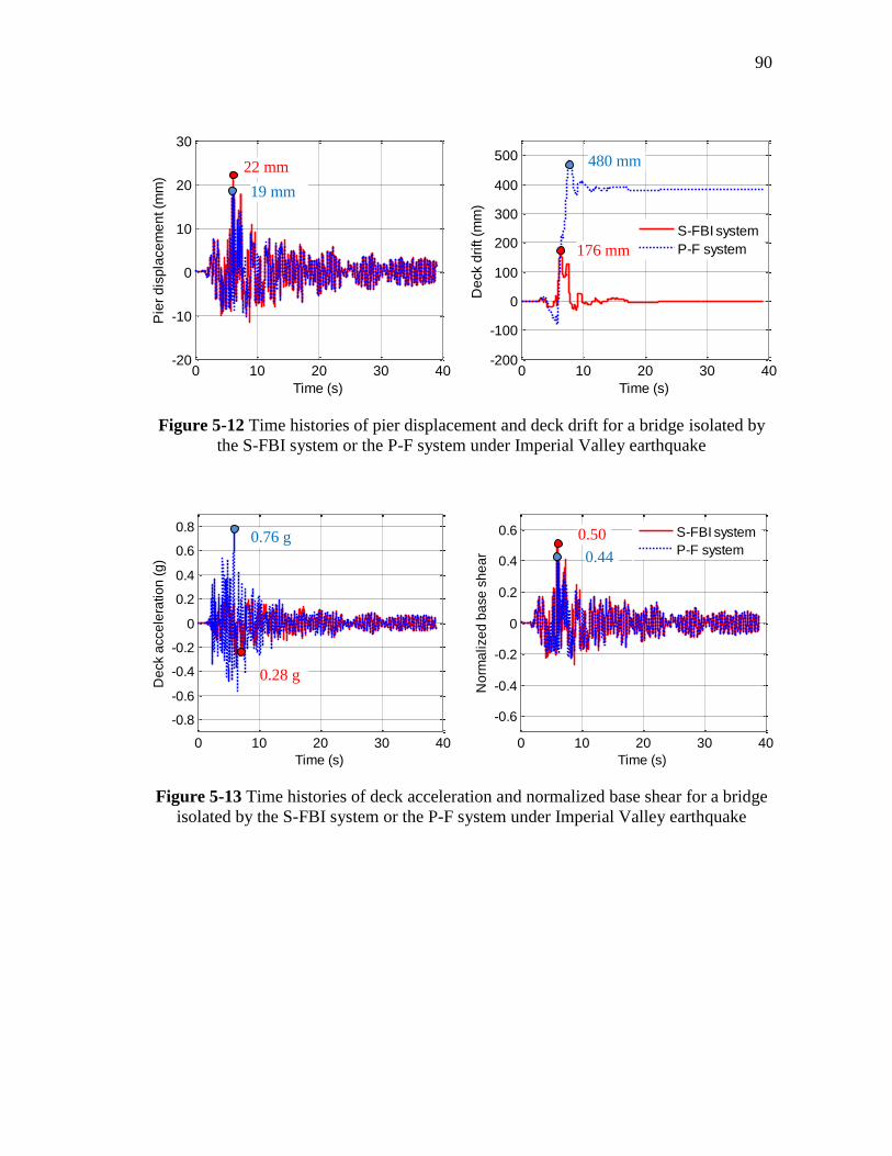
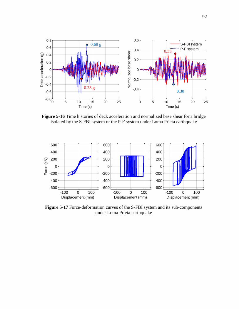
5.5.5 Time Histories of Response Quantities ........................................... 88
5.6 Closure ........................................................................................................... 93
6. SHAPE MEMORY ALLOY/RUBBER-BASED ISOLATION SYSTEM ............. 95
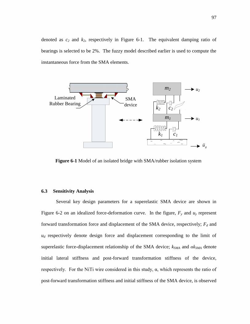
6.1 Introduction .................................................................................................... 95 6.2 Model of Isolated Bridge Structure ................................................................ 96
6.3 Sensitivity Analysis ........................................................................................ 97 6.4 Results of Sensitivity Analysis ....................................................................... 99
6.4.1 Effect of Normalized Forward Transformation Strength of the
SMA Device Fo ............................................................................... 99 6.4.2 Effect of Normalized Forward Transformation Displacement
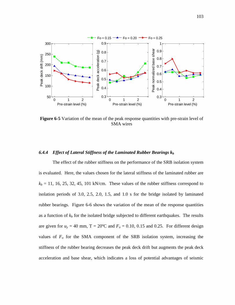
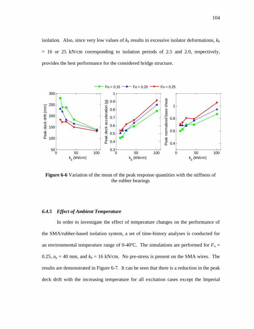
of the SMA Device uy ................................................................... 100 6.4.3 Effect of Pre-Strain Level of the SMA Wires ............................... 102 6.4.4 Effect of Lateral Stiffness of the Laminated Rubber Bearings kb . 103
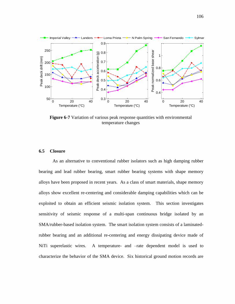
6.4.5 Effect of Ambient Temperature .................................................... 104 6.5 Closure ......................................................................................................... 106
7. SEISMIC PERFORMANCE ASSESSMENT OF SMA-BASED ISOLATION
SYSTEMS USING ENERGY METHODS ........................................................... 109
7.1 Introduction .................................................................................................. 109 7.2 Seismic Input Energy Formulations for Non-Isolated Bridge ..................... 110
7.3 Seismic Input Energy Formulations for Isolated Bridge .............................. 116 7.4 Numerical Study ........................................................................................... 117 7.5 Results .......................................................................................................... 118
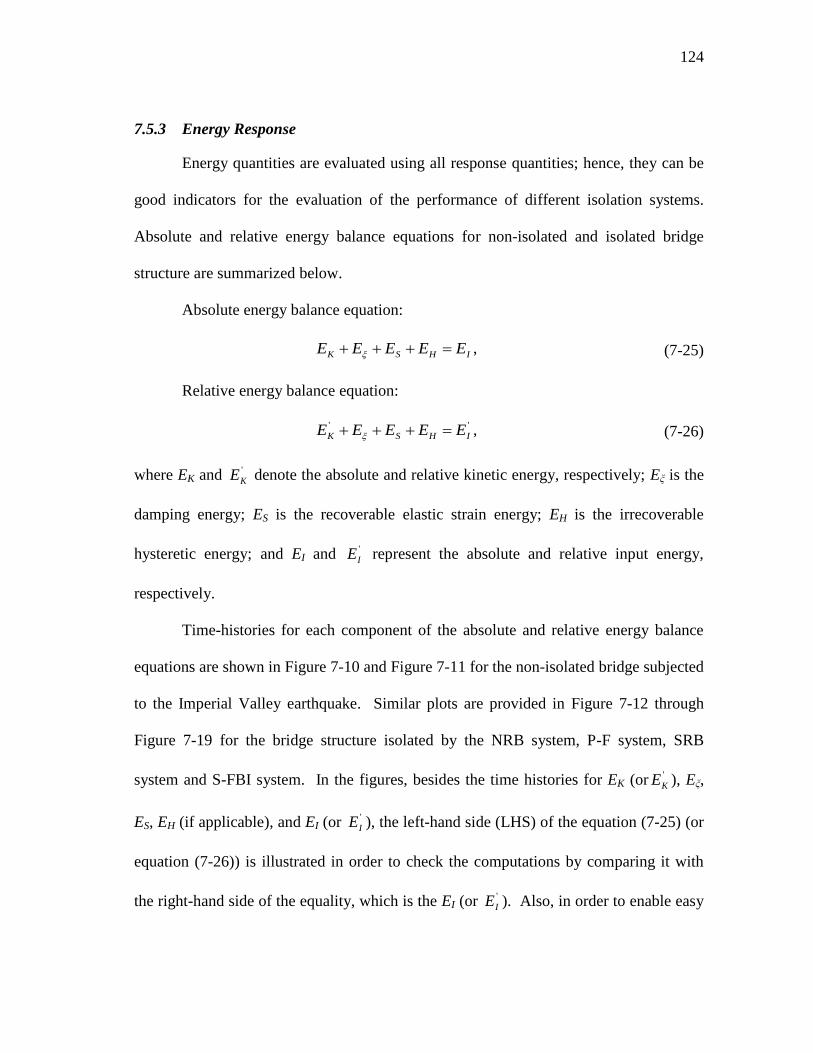
7.5.1 Peak Structural Response .............................................................. 118 7.5.2 Time Histories of Structural Response .......................................... 120 7.5.3 Energy Response ........................................................................... 124
7.6 Closure ......................................................................................................... 135
8. A COMPARATIVE STUDY ON SEISMIC PERFORMANCE OF
SUPERELASTIC-FRICTION BASE ISOLATORS ............................................ 137
8.1 Introduction .................................................................................................. 137 8.2 Model of Isolated Bridge Structure .............................................................. 137
Page 11
x
Page
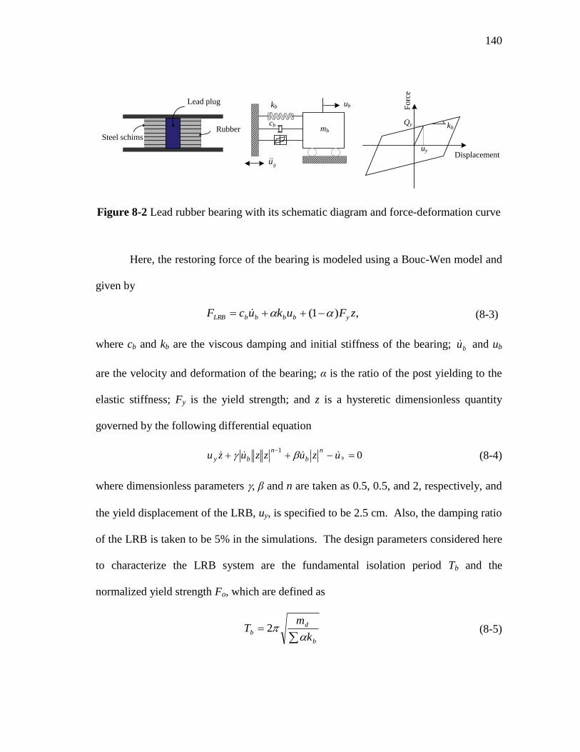
8.3 Modeling of Seismic Isolation Systems ....................................................... 139
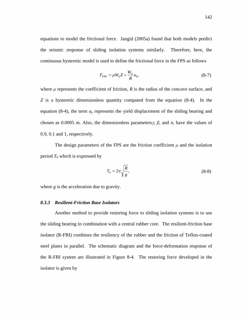
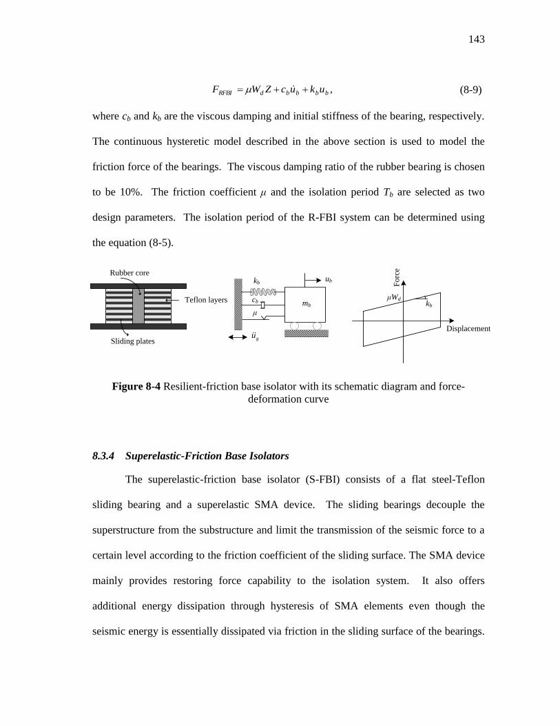
8.3.1 Lead Rubber Bearings ................................................................... 139 8.3.2 Friction Pendulum Systems ........................................................... 141 8.3.3 Resilient-Friction Base Isolators ................................................... 142 8.3.4 Superelastic-Friction Base Isolators .............................................. 143
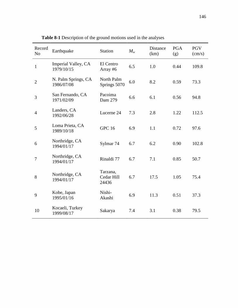
8.4 Ground Motions Used for Analyses ............................................................. 145
8.5 Parametric Study .......................................................................................... 147 8.5.1 Comparative Performance Study .................................................. 147 8.5.2 Sensitivity Analysis ....................................................................... 152
8.6 Closure ......................................................................................................... 155
9. EVALUATION OF THE PERFORMANCE OF THE S-FBI SYSTEM
CONSIDERING TEMPERATURE EFFECTS ..................................................... 157
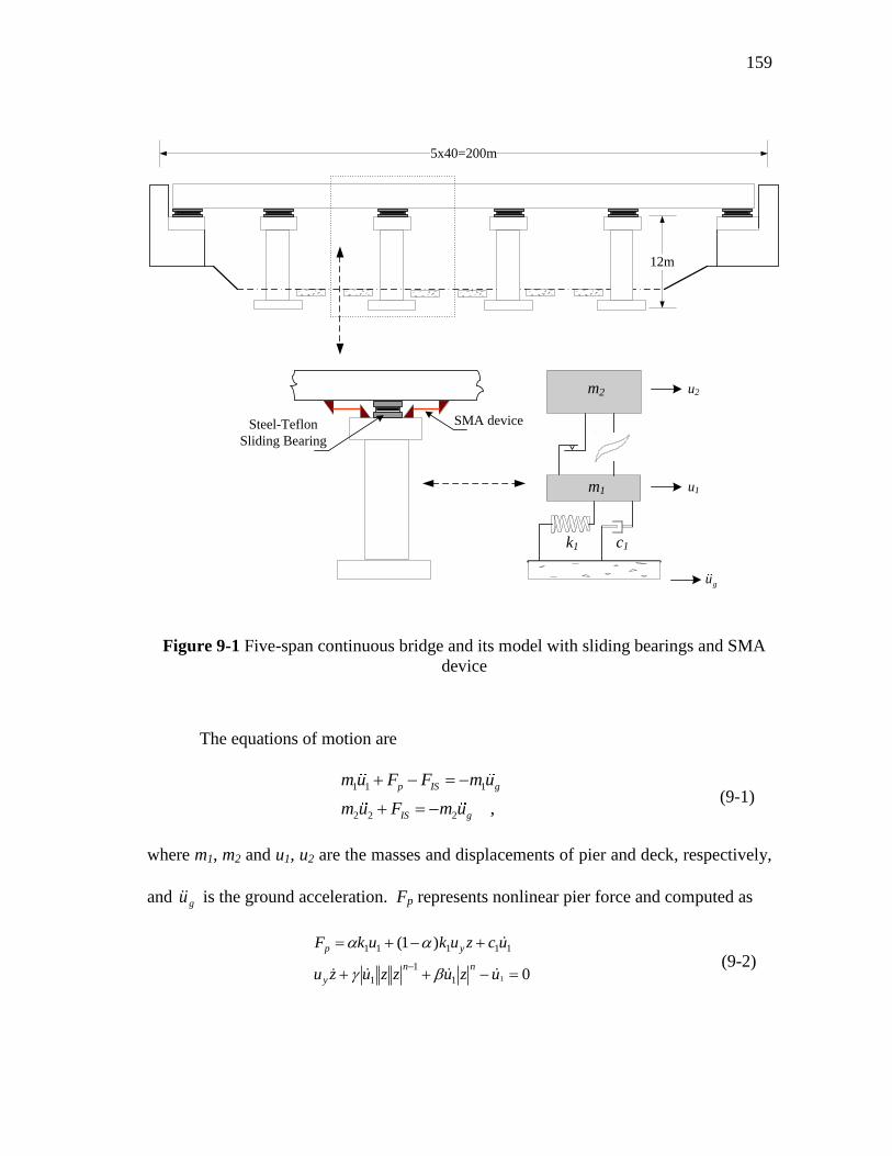
9.1 Introduction .................................................................................................. 157 9.2 Model of Isolated Bridge Structure .............................................................. 158
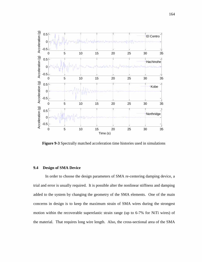
9.3 Ground Motions Used for Analyses ............................................................. 161 9.4 Design of SMA Device ................................................................................ 164
9.5 Results .......................................................................................................... 166 9.6 Closure ......................................................................................................... 177
10. SUMMARY, CONCLUSIONS AND RECOMMENDATIONS .......................... 179
REFERENCES ............................................................................................................... 182
VITA .............................................................................................................................. 197
Page 12
xi
LIST OF FIGURES
Page
Figure 2-1 Different phases of shape memory alloys........................................................ 8
Figure 2-2 Martensite fraction-temperature diagram of SMAs ........................................ 9
Figure 2-3 Shape memory effect ..................................................................................... 10
Figure 2-4 Superelastic effect ......................................................................................... 12
Figure 2-5 Results of cyclic tensile tests on NiTi wires (Malecot et al., 2006) .............. 17
Figure 2-6 Stress-strain curves of NiTi wires at different temperatures (Churchill et
al., 2009) ....................................................................................................... 20
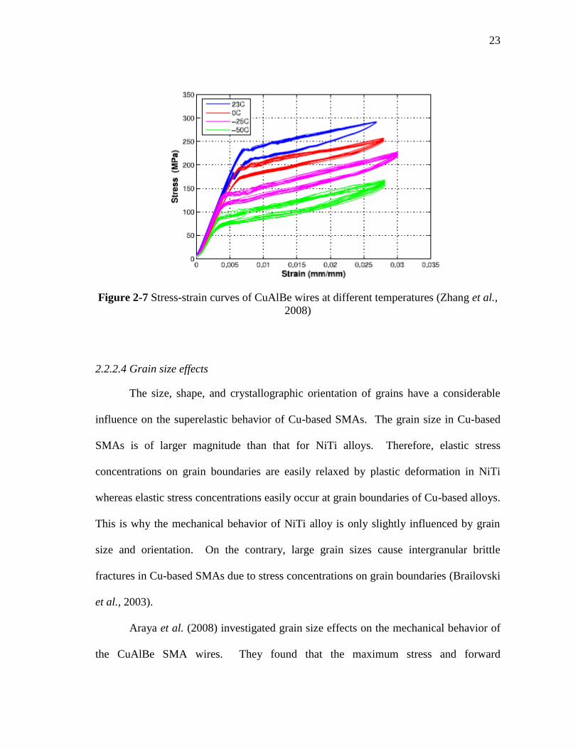
Figure 2-7 Stress-strain curves of CuAlBe wires at different temperatures (Zhang et
al., 2008) ....................................................................................................... 23
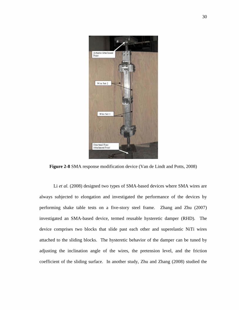
Figure 2-8 SMA response modification device (Van de Lindt and Potts, 2008) ............ 30
Figure 2-9 SMA tension/compression device (Speicher et al., 2009) ............................ 31
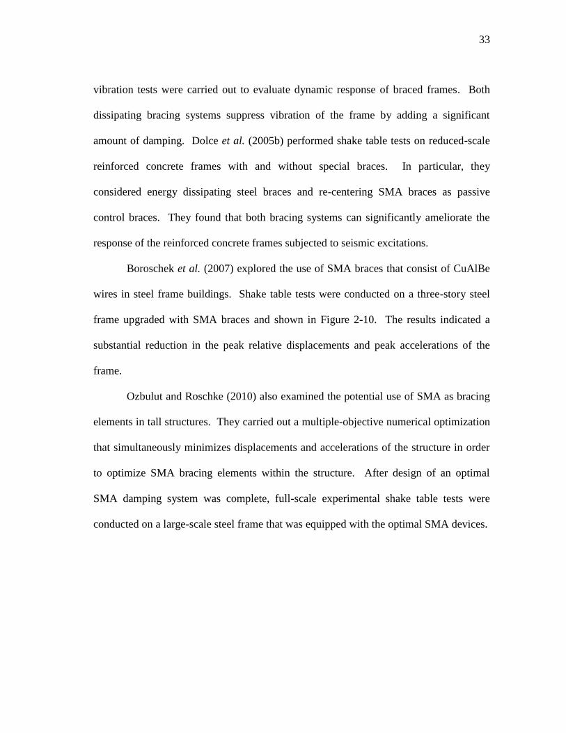
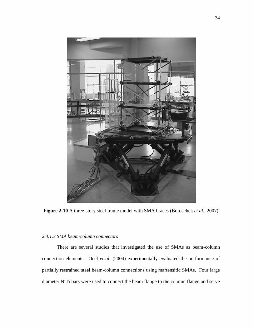
Figure 2-10 A three-story steel frame model with SMA braces (Boroschek et al.,
2007) ............................................................................................................. 34
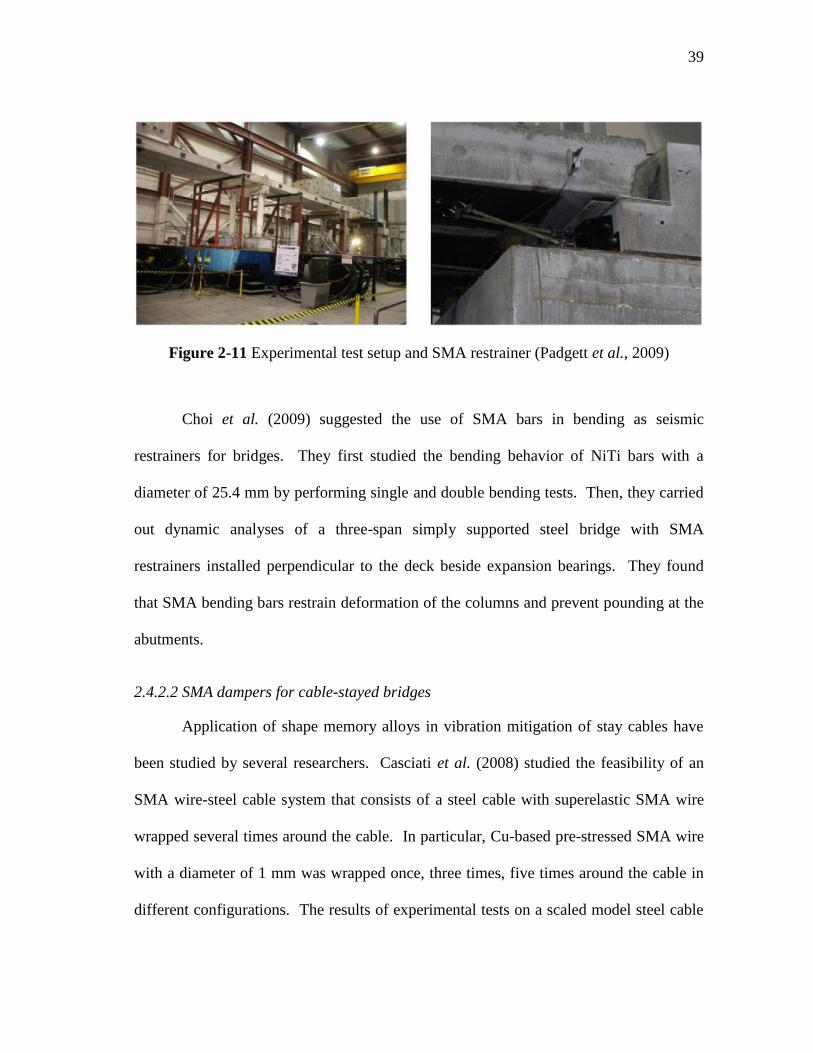
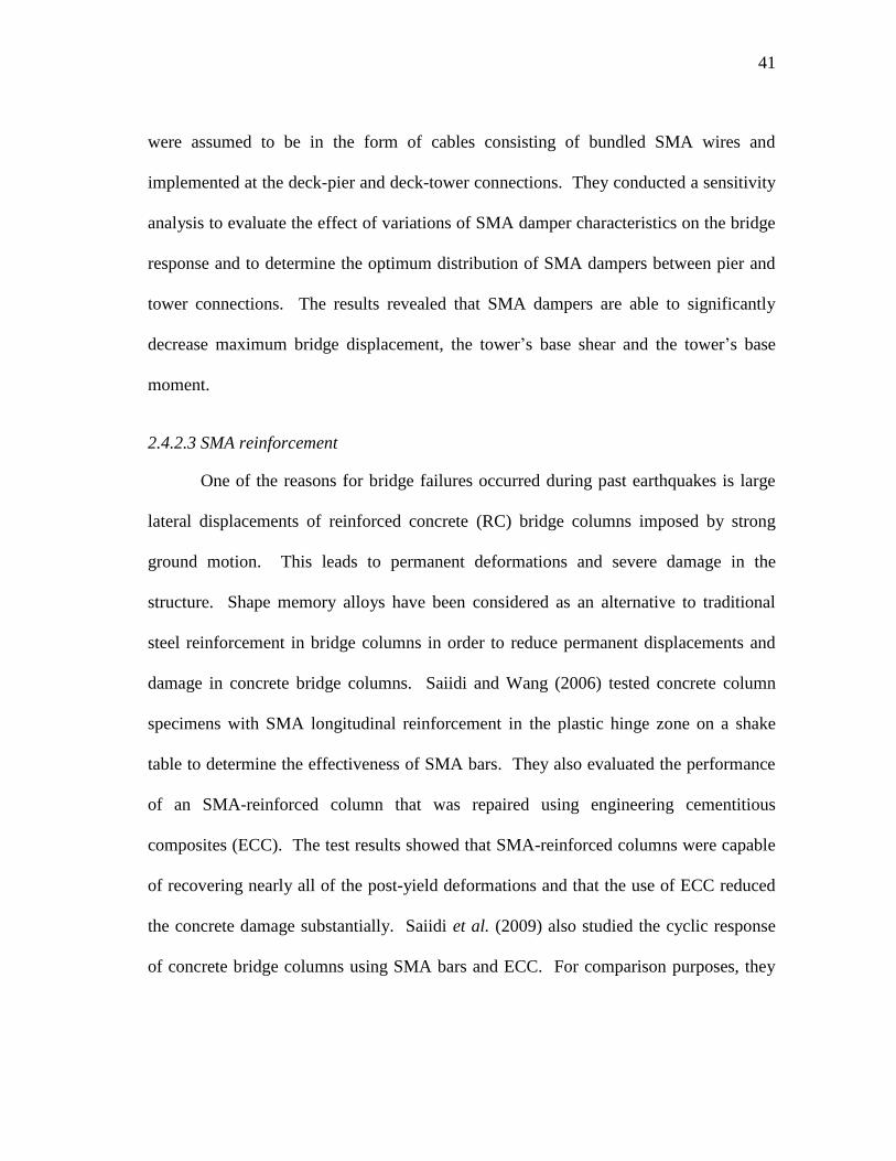
Figure 2-11 Experimental test setup and SMA restrainer (Padgett et al., 2009) ............. 39
Figure 2-12 Concrete specimen with SMA spirals (Andrawes et al., 2010) ................... 42
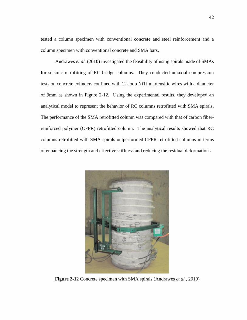
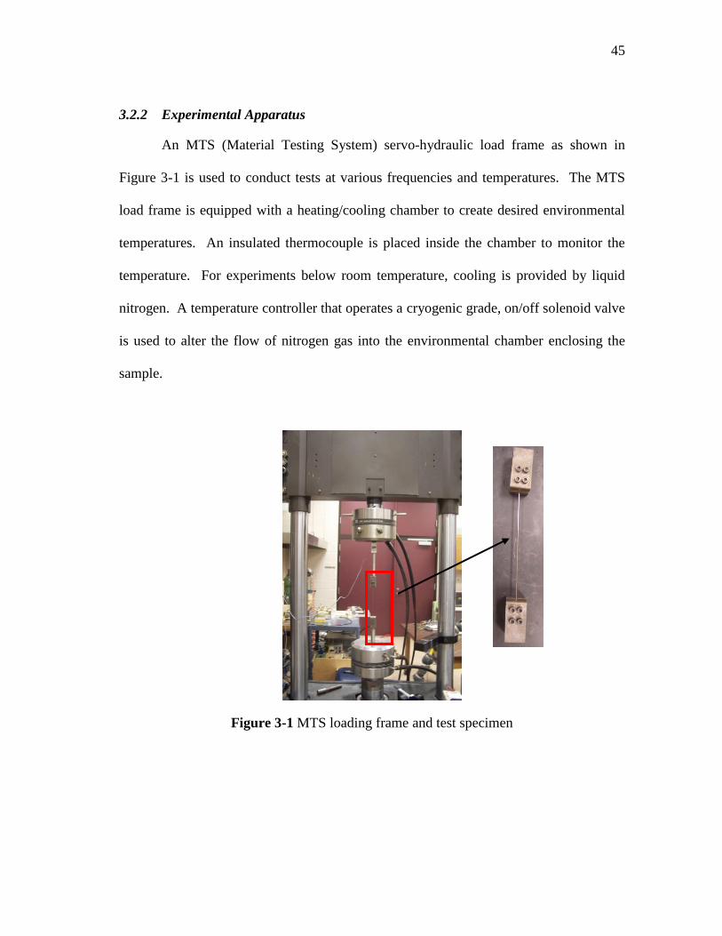
Figure 3-1 MTS loading frame and test specimen .......................................................... 45
Figure 3-2 Hysteresis loops of superelastic SMA wires for 1st, 2
nd, and 3
rd loading
cycles ............................................................................................................. 47
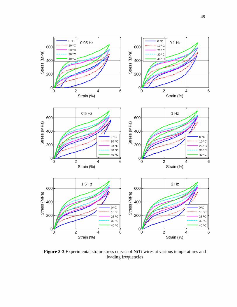
Figure 3-3 Experimental strain-stress curves of NiTi wires at various temperatures
and loading frequencies................................................................................. 49
Figure 3-4 Energy dissipation, equivalent viscous damping and secant stiffness of
NiTi wires as a function of temperature at different loading frequencies ..... 50
Page 13
xii
Page
Figure 3-5 Experimental strain-stress curves of NiTi wires at various temperatures
and loading frequencies................................................................................. 52
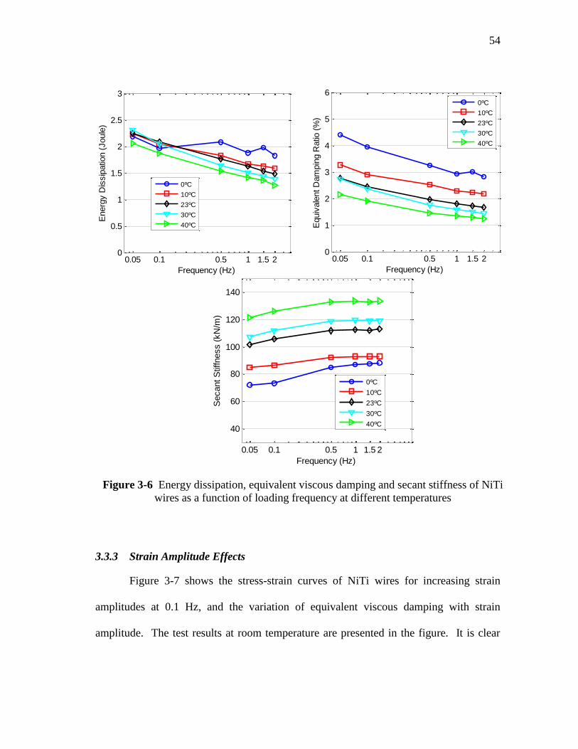
Figure 3-6 Energy dissipation, equivalent viscous damping and secant stiffness of
NiTi wires as a function of loading frequency at different temperatures ..... 54
Figure 3-7 Experimental strain-stress curves of NiTi wires at various strain
amplitudes, and equivalent viscous damping as a function of strain
amplitude ....................................................................................................... 55
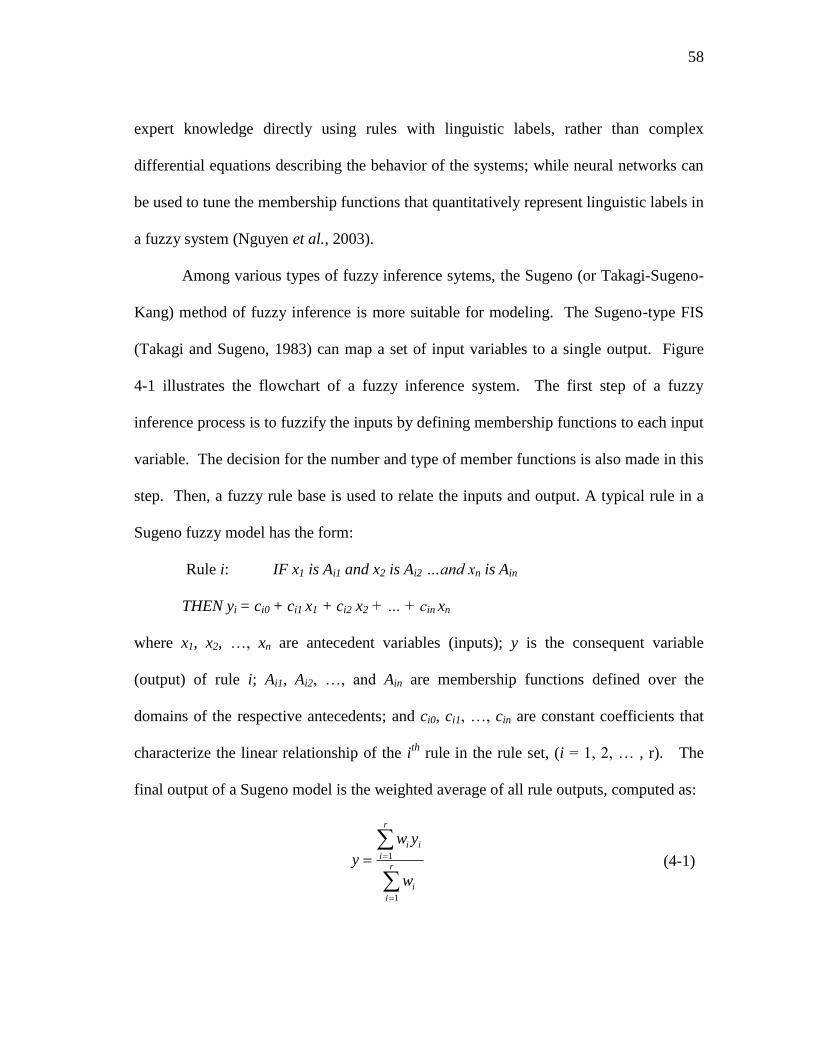
Figure 4-1 Flowchart of a fuzzy inference system .......................................................... 59
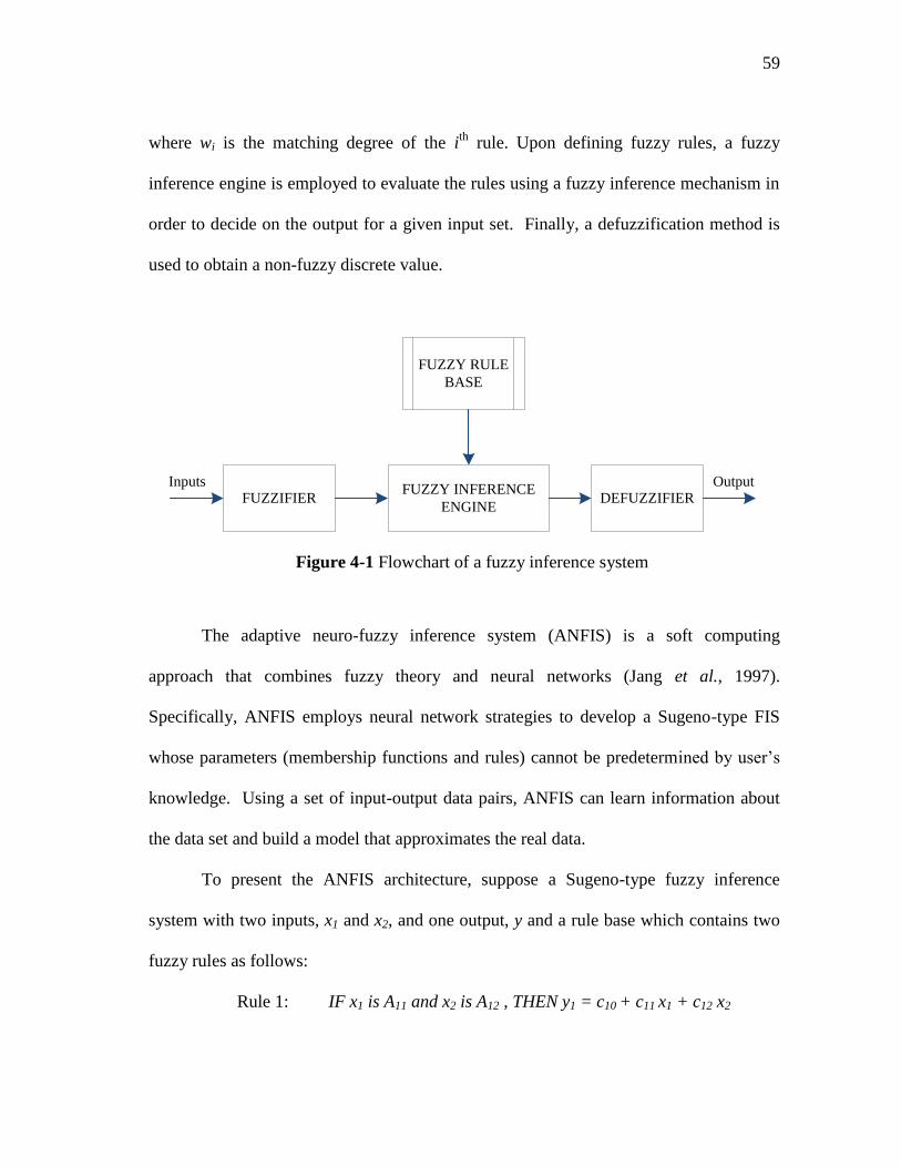
Figure 4-2 ANFIS scheme for two-input Sugeno-type fuzzy model .............................. 61
Figure 4-3 Fuzzy inference system with its inputs and output ........................................ 63
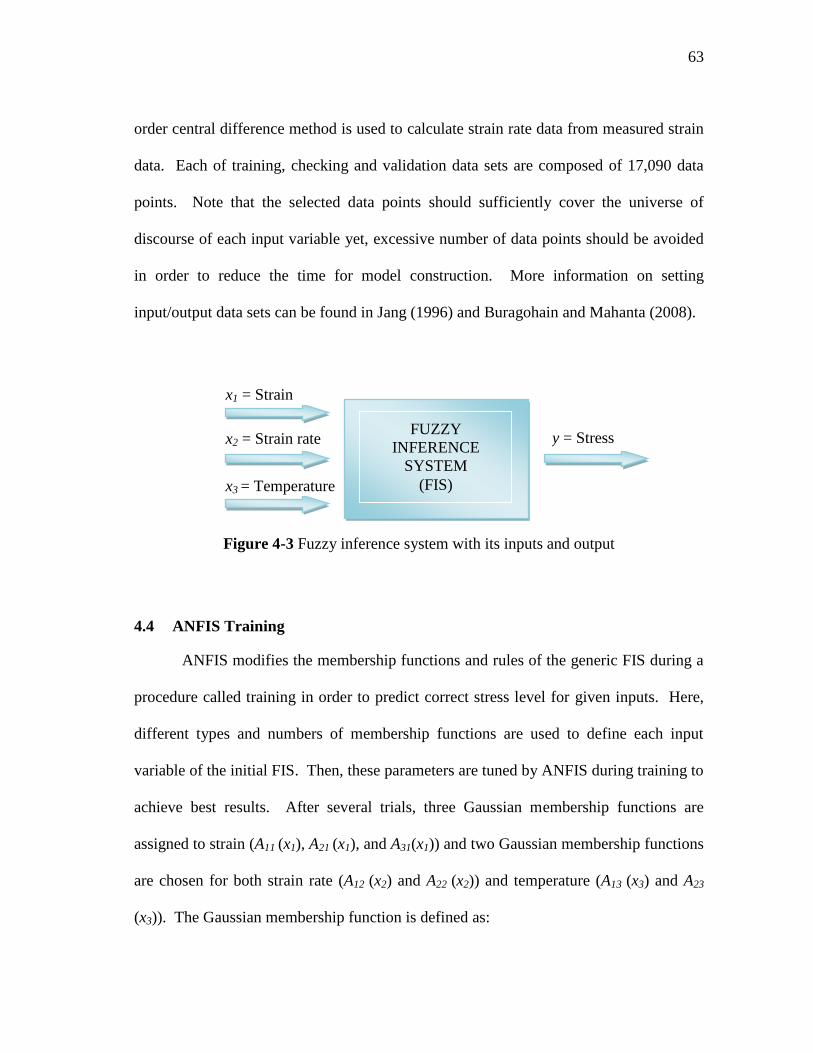
Figure 4-4 Initial and final membership function of FIS ................................................ 65
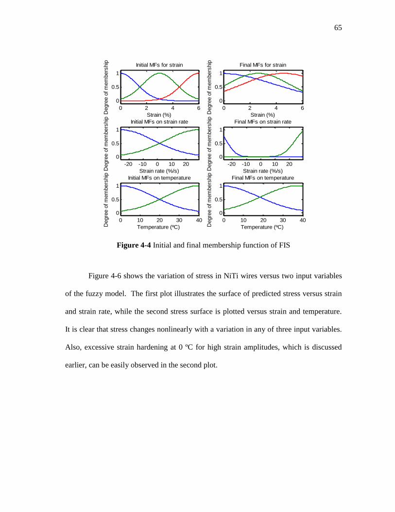
Figure 4-5 Experimental input data and, measured and predicted stress ........................ 66
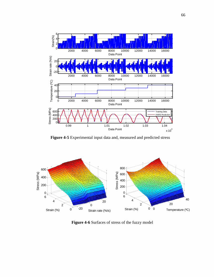
Figure 4-6 Surfaces of stress of the fuzzy model ............................................................ 66
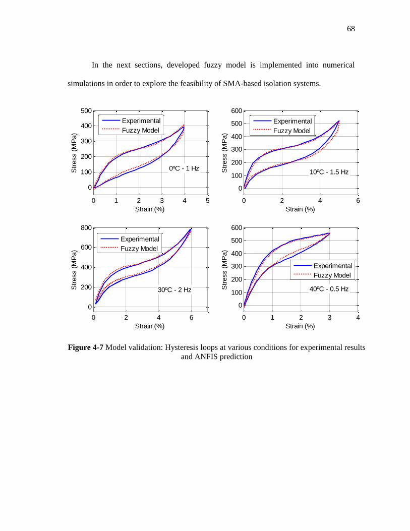
Figure 4-7 Model validation: Hysteresis loops at various conditions for
experimental results and ANFIS prediction .................................................. 68
Figure 5-1 Model of a three-span isolated bridge ........................................................... 72
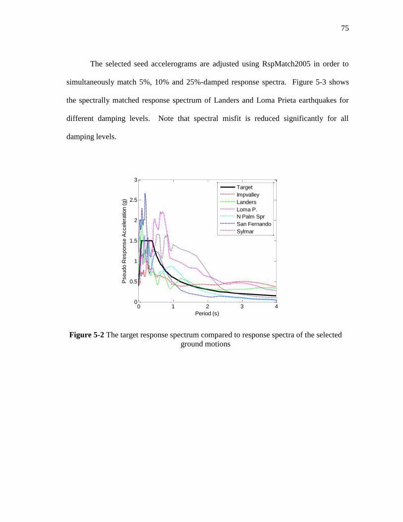
Figure 5-2 The target response spectrum compared to response spectra of the
selected ground motions ................................................................................ 75
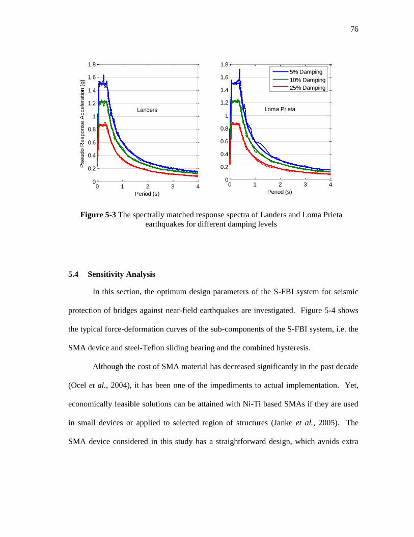
Figure 5-3 The spectrally matched response spectra of Landers and Loma Prieta
earthquakes for different damping levels ...................................................... 76
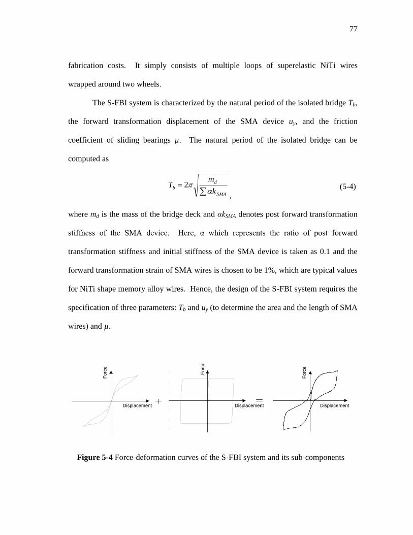
Figure 5-4 Force-deformation curves of the S-FBI system and its sub-components ...... 77
Figure 5-5 Variations of peak response quantities with the natural period of the
isolated bridge ............................................................................................... 79
Figure 5-6 Variation of peak response quantities with friction coefficient of sliding
bearings ......................................................................................................... 80
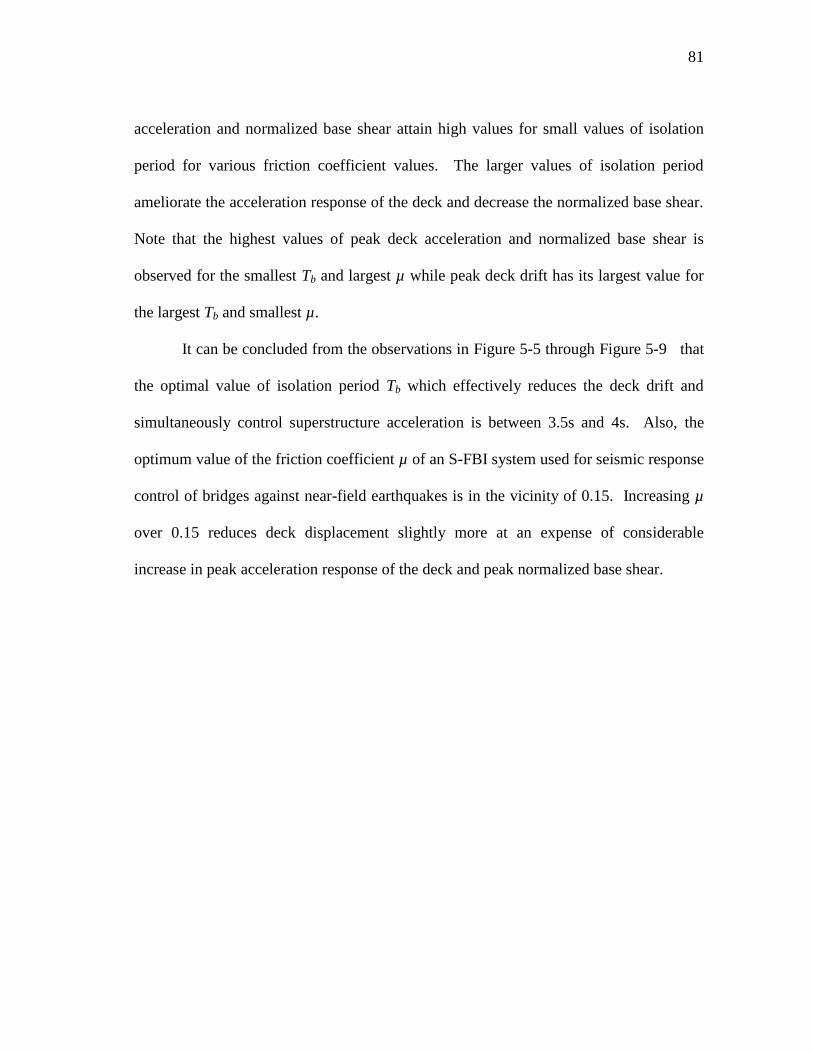
Figure 5-7 Variations of peak deck drift with isolation period and friction coefficient . 82
Page 14
xiii
Page
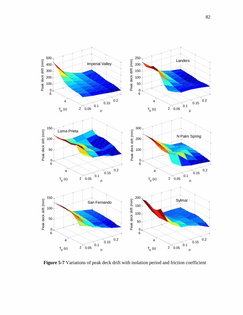
Figure 5-8 Variations of peak deck acceleration with isolation period and friction
coefficient ...................................................................................................... 83
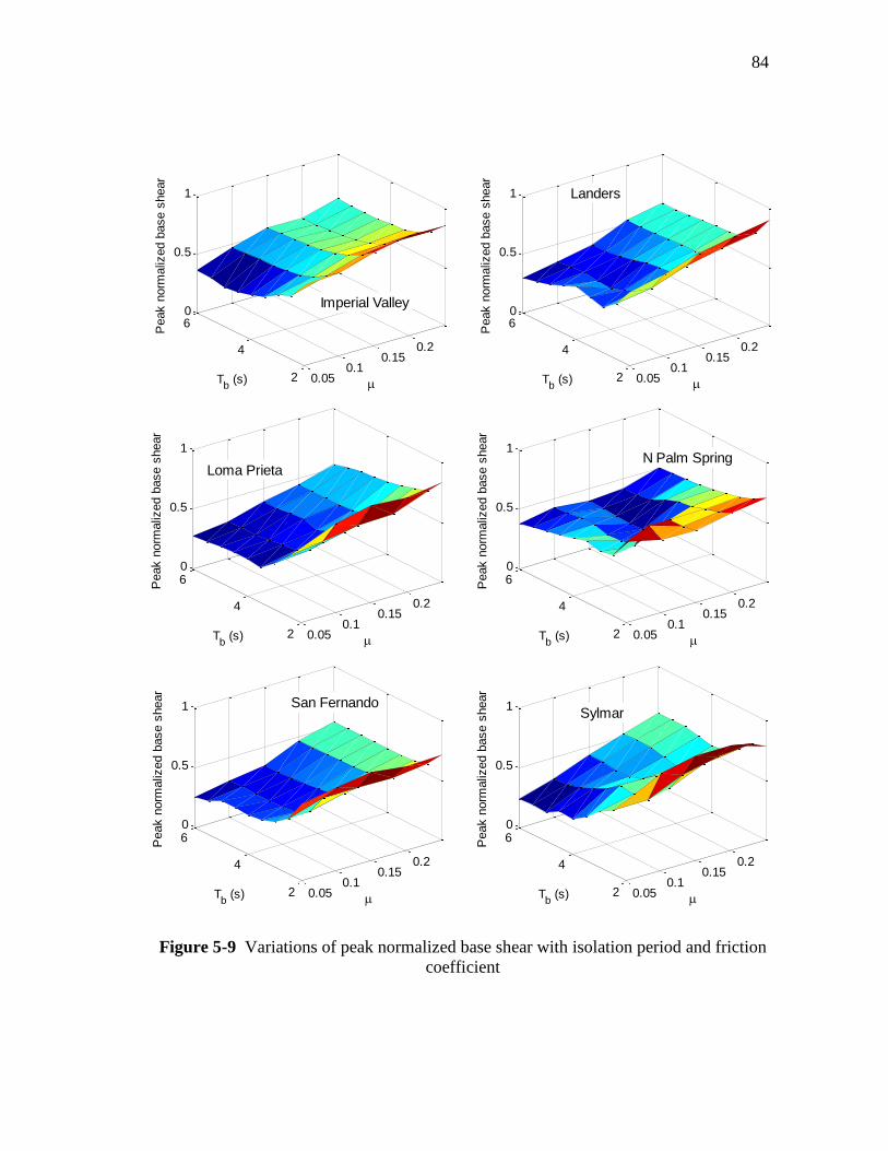
Figure 5-9 Variations of peak normalized base shear with isolation period and
friction coefficient ........................................................................................ 84
Figure 5-10 Variations of peak response quantities with forward transformation
displacement of the SMA device .................................................................. 86
Figure 5-11 Variations of peak response quantities with environmental temperature ..... 88
Figure 5-12 Time histories of pier displacement and deck drift for a bridge isolated
by the S-FBI system or the P-F system under Imperial Valley earthquake . 90
Figure 5-13 Time histories of deck acceleration and normalized base shear for a
bridge isolated by the S-FBI system or the P-F system under Imperial
Valley earthquake ......................................................................................... 90
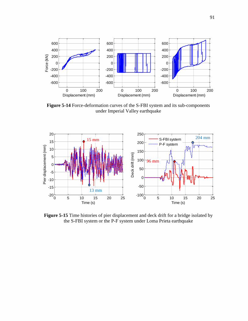
Figure 5-14 Force-deformation curves of the S-FBI system and its sub-components
under Imperial Valley earthquake ................................................................ 91
Figure 5-15 Time histories of pier displacement and deck drift for a bridge isolated
by the S-FBI system or the P-F system under Loma Prieta earthquake ....... 91
Figure 5-16 Time histories of deck acceleration and normalized base shear for a
bridge isolated by the S-FBI system or the P-F system under Loma
Prieta earthquake .......................................................................................... 92
Figure 5-17 Force-deformation curves of the S-FBI system and its sub-components
under Loma Prieta earthquake ...................................................................... 92
Figure 6-1 Model of an isolated bridge with SMA/rubber isolation system ................... 97
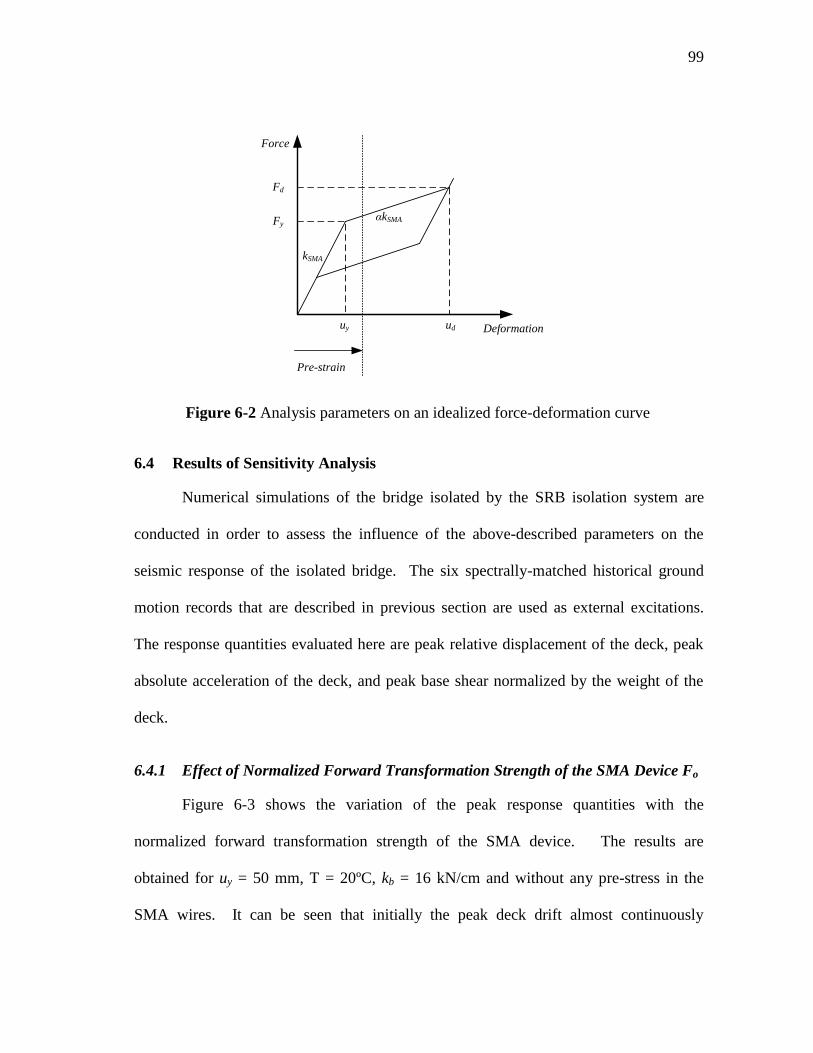
Figure 6-2 Analysis parameters on an idealized force-deformation curve ..................... 99
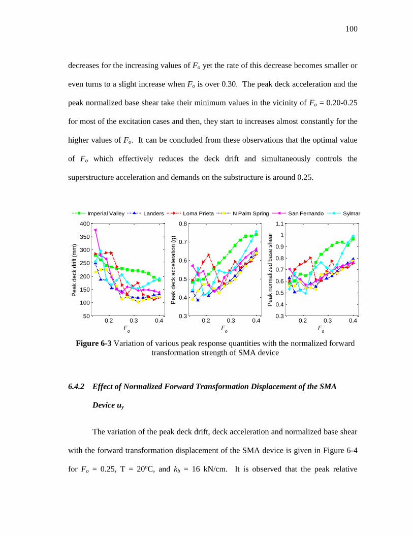
Figure 6-3 Variation of various peak response quantities with the normalized
forward transformation strength of SMA device ........................................ 100
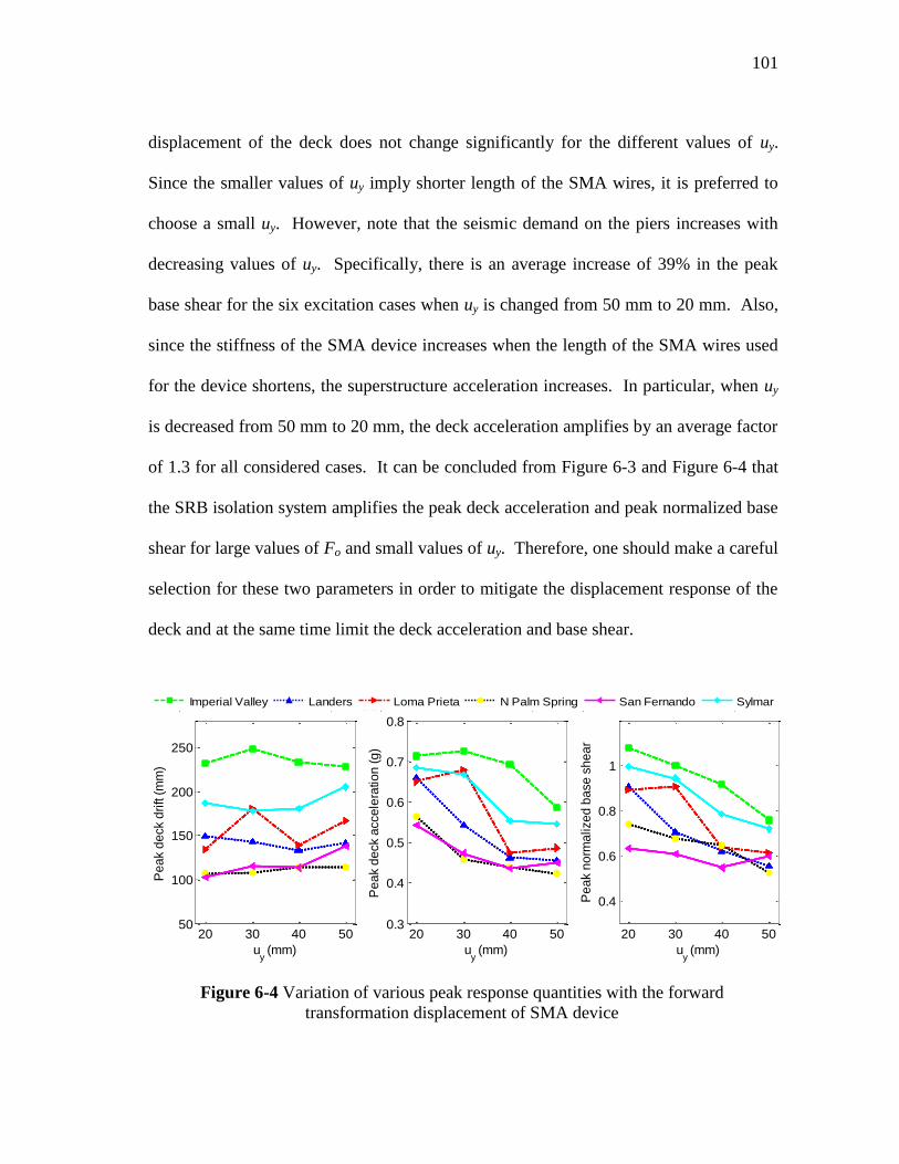
Figure 6-4 Variation of various peak response quantities with the forward
transformation displacement of SMA device ............................................. 101
Page 15
xiv
Page
Figure 6-5 Variation of the mean of the peak response quantities with pre-strain
level of SMA wires ..................................................................................... 103
Figure 6-6 Variation of the mean of the peak response quantities with the stiffness
of the rubber bearings ................................................................................. 104
Figure 6-7 Variation of various peak response quantities with environmental
temperature changes .................................................................................... 106
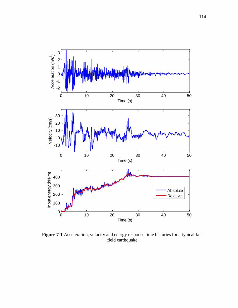
Figure 7-1 Acceleration, velocity and energy response time histories for a typical
far-field earthquake ..................................................................................... 114
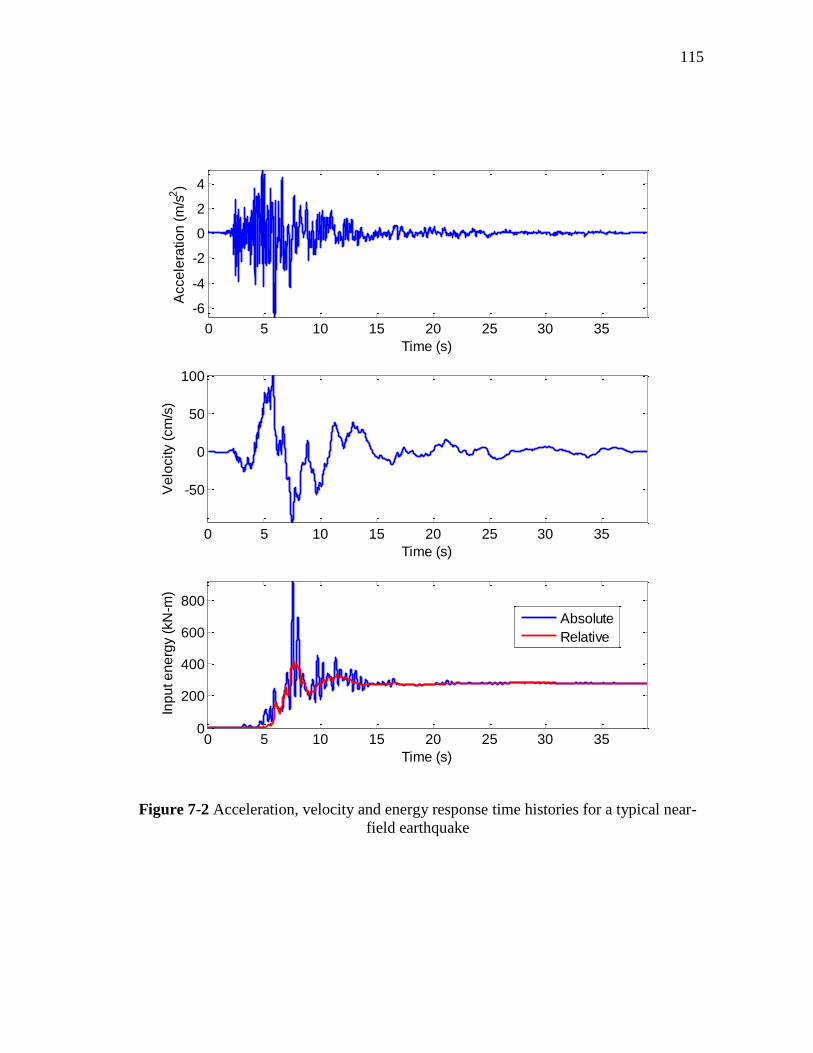
Figure 7-2 Acceleration, velocity and energy response time histories for a typical
near-field earthquake ................................................................................... 115
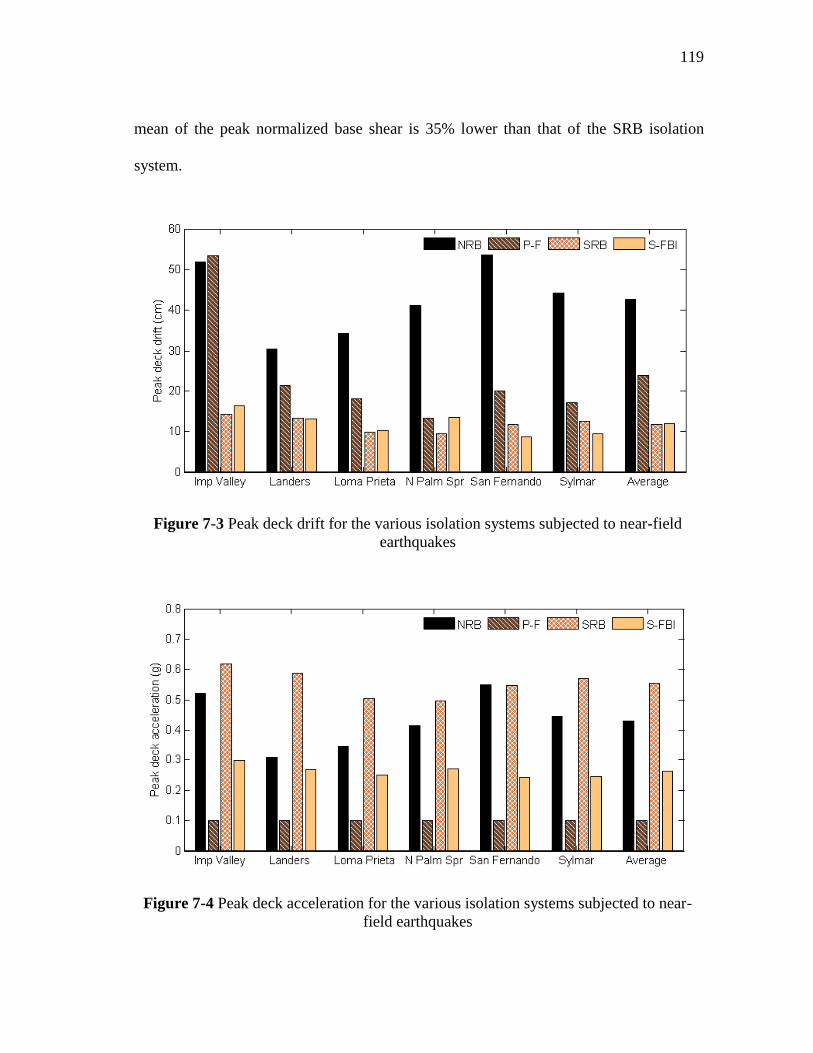
Figure 7-3 Peak deck drift for the various isolation systems subjected to near-field
earthquakes .................................................................................................. 119
Figure 7-4 Peak deck acceleration for the various isolation systems subjected to
near-field earthquakes ................................................................................. 119
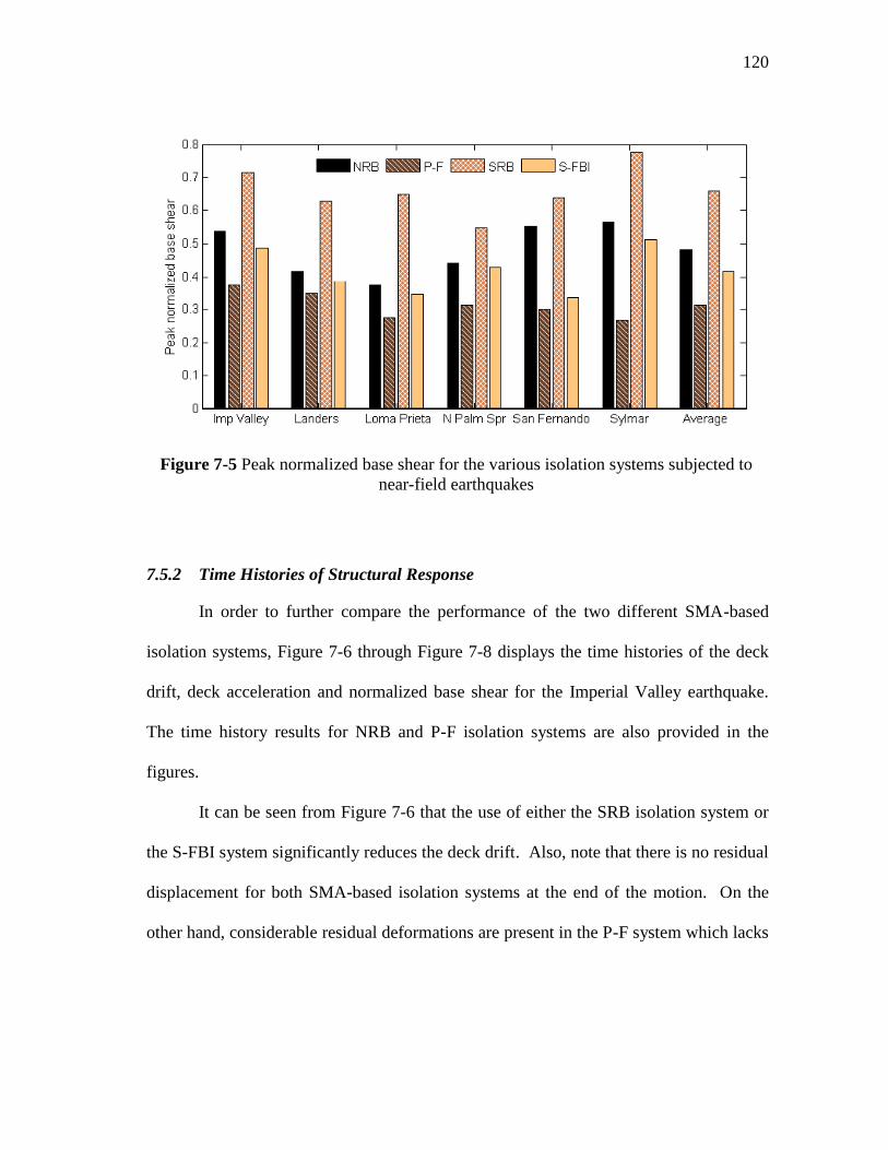
Figure 7-5 Peak normalized base shear for the various isolation systems subjected
to near-field earthquakes ............................................................................. 120
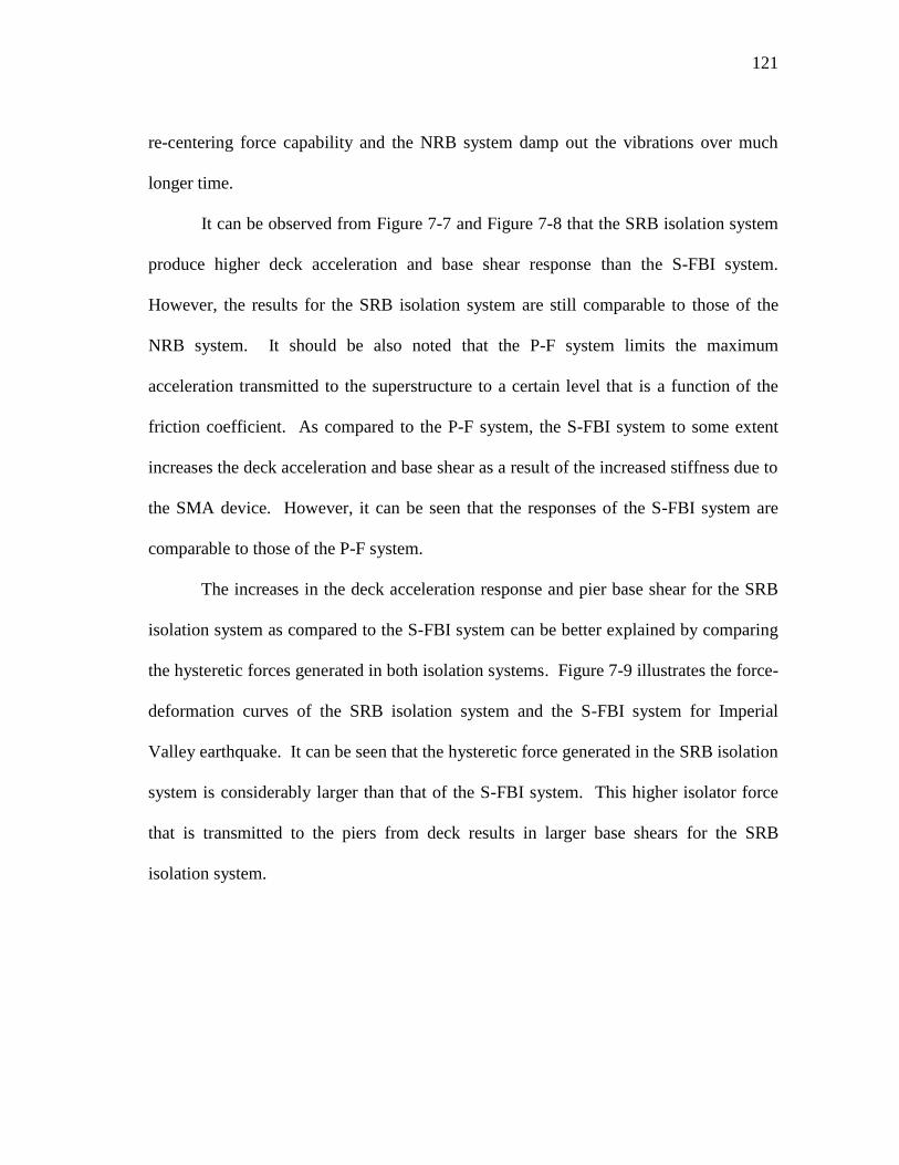
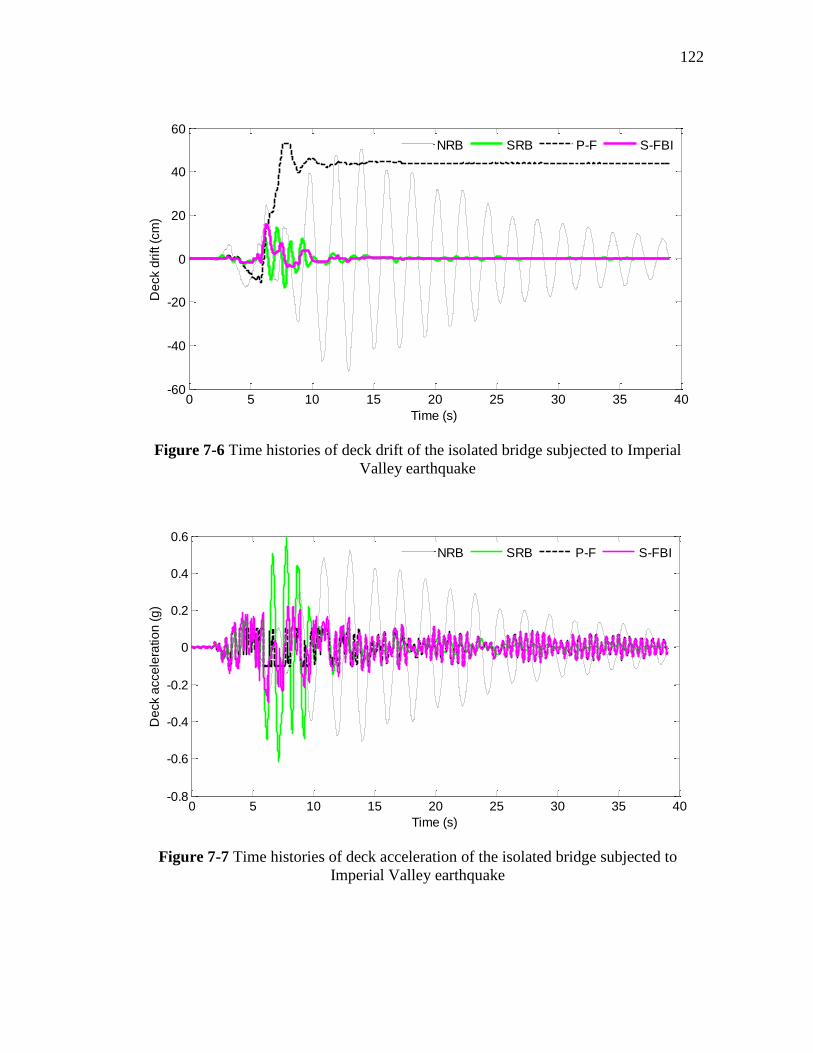
Figure 7-6 Time histories of deck drift of the isolated bridge subjected to Imperial
Valley earthquake........................................................................................ 122
Figure 7-7 Time histories of deck acceleration of the isolated bridge subjected to
Imperial Valley earthquake ......................................................................... 122
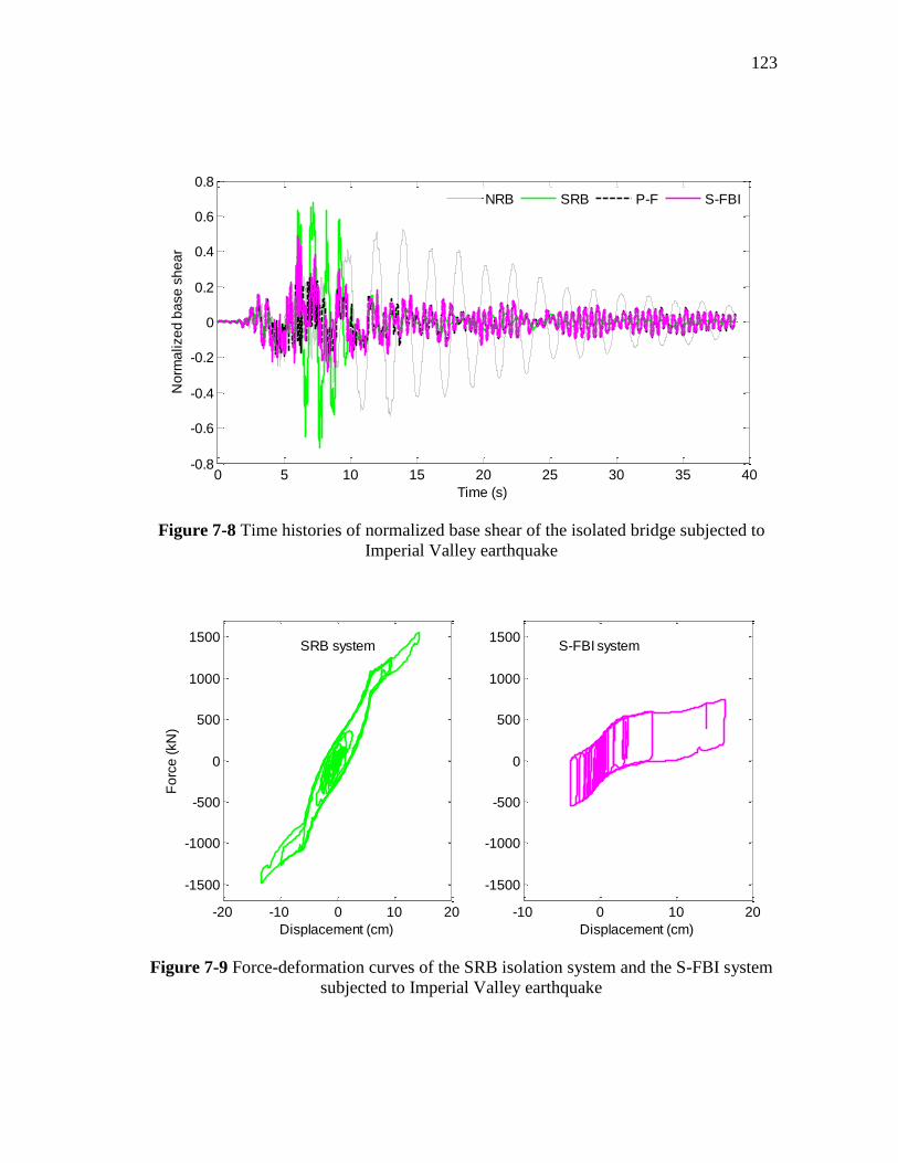
Figure 7-8 Time histories of normalized base shear of the isolated bridge
subjected to Imperial Valley earthquake ..................................................... 123
Figure 7-9 Force-deformation curves of the SRB isolation system and the S-FBI
system subjected to Imperial Valley earthquake ......................................... 123
Figure 7-10 Energy time histories for the non-isolated bridge subjected to Imperial
Valley earthquake for absolute energy formulation ................................... 126
Page 16
xv
Page
Figure 7-11 Energy time histories for the non-isolated bridge subjected to Imperial
Valley earthquake for relative energy formulation ..................................... 126
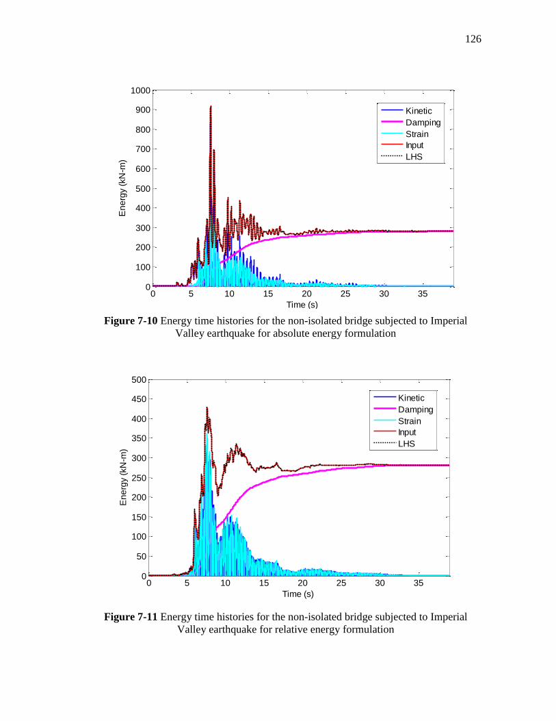
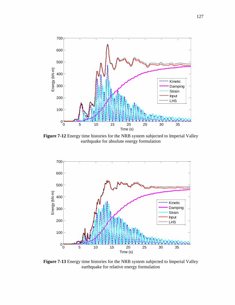
Figure 7-12 Energy time histories for the NRB system subjected to Imperial Valley
earthquake for absolute energy formulation ............................................... 127
Figure 7-13 Energy time histories for the NRB system subjected to Imperial Valley
earthquake for relative energy formulation ................................................ 127
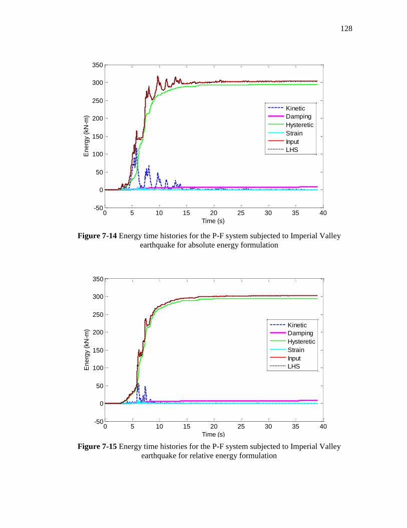
Figure 7-14 Energy time histories for the P-F system subjected to Imperial Valley
earthquake for absolute energy formulation ............................................... 128
Figure 7-15 Energy time histories for the P-F system subjected to Imperial Valley
earthquake for relative energy formulation ................................................ 128
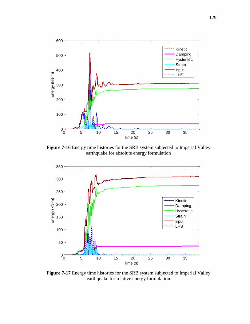
Figure 7-16 Energy time histories for the SRB system subjected to Imperial Valley
earthquake for absolute energy formulation ............................................... 129
Figure 7-17 Energy time histories for the SRB system subjected to Imperial Valley
earthquake for relative energy formulation ................................................ 129
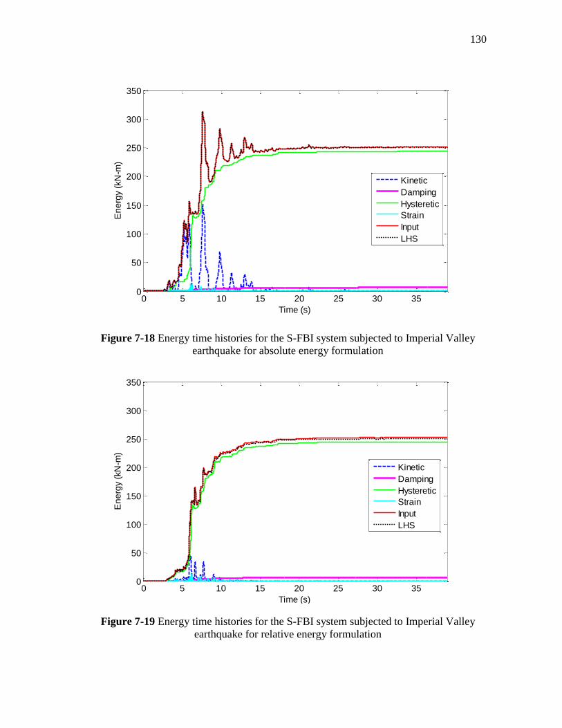
Figure 7-18 Energy time histories for the S-FBI system subjected to Imperial
Valley earthquake for absolute energy formulation ................................... 130
Figure 7-19 Energy time histories for the S-FBI system subjected to Imperial
Valley earthquake for relative energy formulation ..................................... 130
Figure 7-20 Time histories of absolute input energy for the non-isolated and
isolated bridge structures subjected to Imperial Valley earthquake ........... 131
Figure 7-21 Time histories of relative input energy for the non-isolated and
isolated bridge structures subjected to Imperial Valley earthquake ........... 131
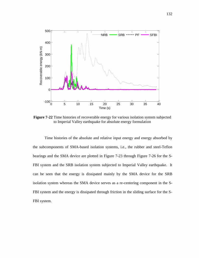
Figure 7-22 Time histories of recoverable energy for various isolation system
subjected to Imperial Valley earthquake for absolute energy formulation 132
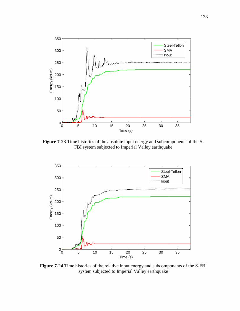
Figure 7-23 Time histories of the absolute input energy and subcomponents of the
S-FBI system subjected to Imperial Valley earthquake ............................. 133
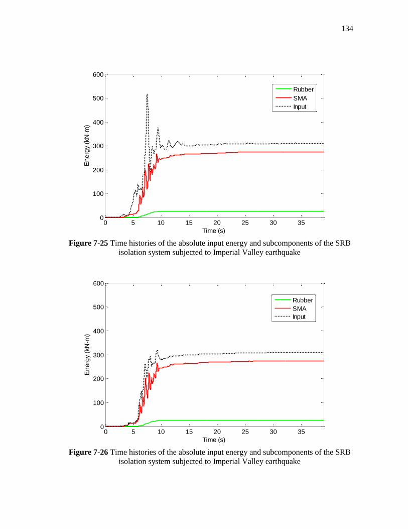
Figure 7-24 Time histories of the relative input energy and subcomponents of the
S-FBI system subjected to Imperial Valley earthquake ............................. 133
Page 17
xvi
Page
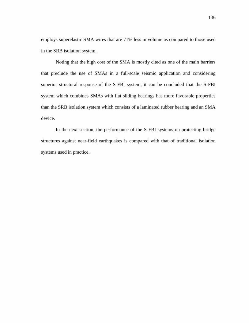
Figure 7-25 Time histories of the absolute input energy and subcomponents of the
SRB isolation system subjected to Imperial Valley earthquake ................. 134
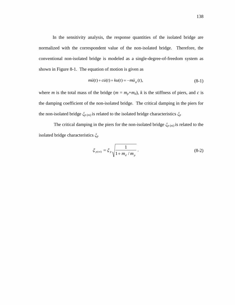
Figure 7-26 Time histories of the absolute input energy and subcomponents of the
SRB isolation system subjected to Imperial Valley earthquake ................. 134
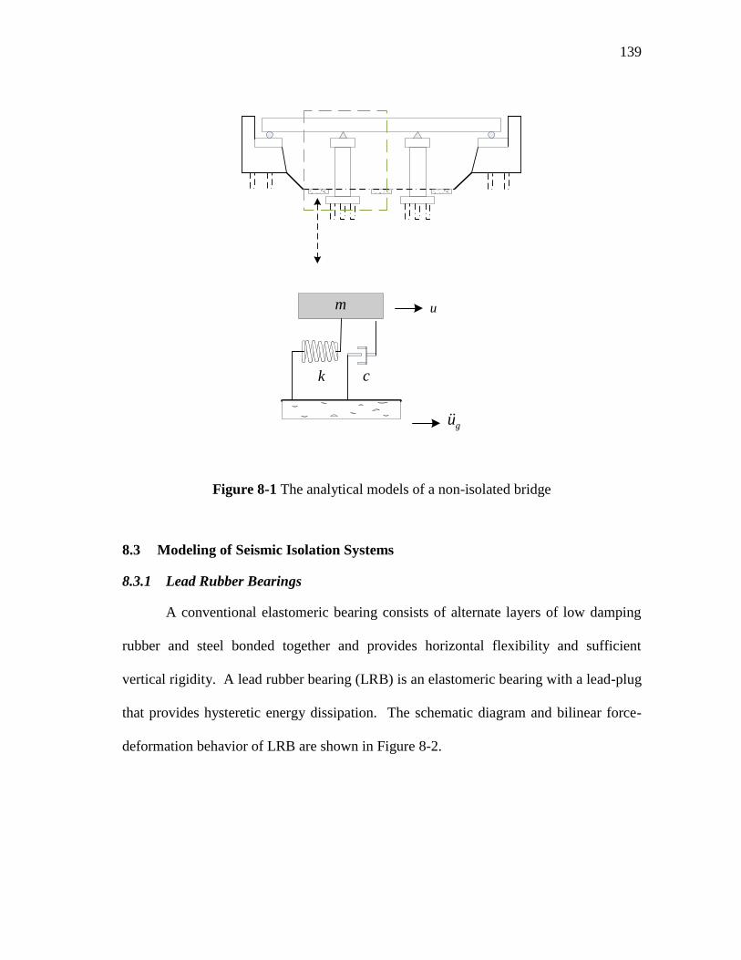
Figure 8-1 The analytical models of a non-isolated bridge ........................................... 139
Figure 8-2 Lead rubber bearing with its schematic diagram and force-deformation
curve ............................................................................................................ 140
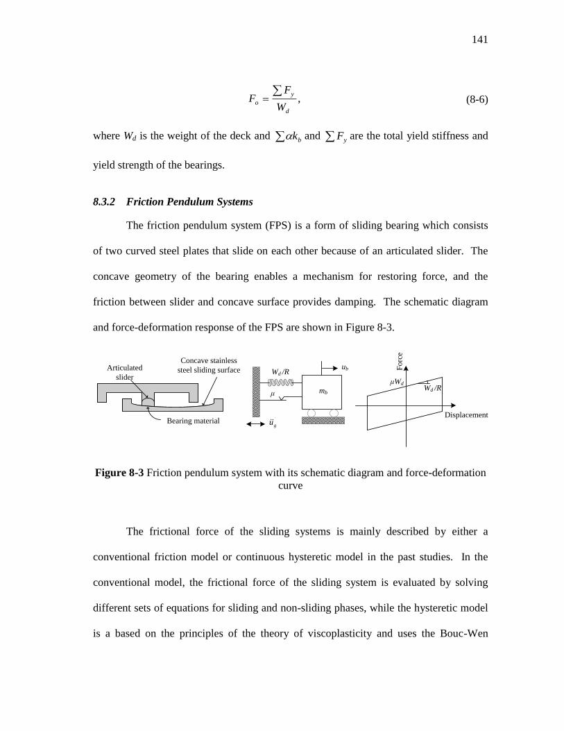
Figure 8-3 Friction pendulum system with its schematic diagram and force-
deformation curve ....................................................................................... 141
Figure 8-4 Resilient-friction base isolator with its schematic diagram and force-
deformation curve ....................................................................................... 143
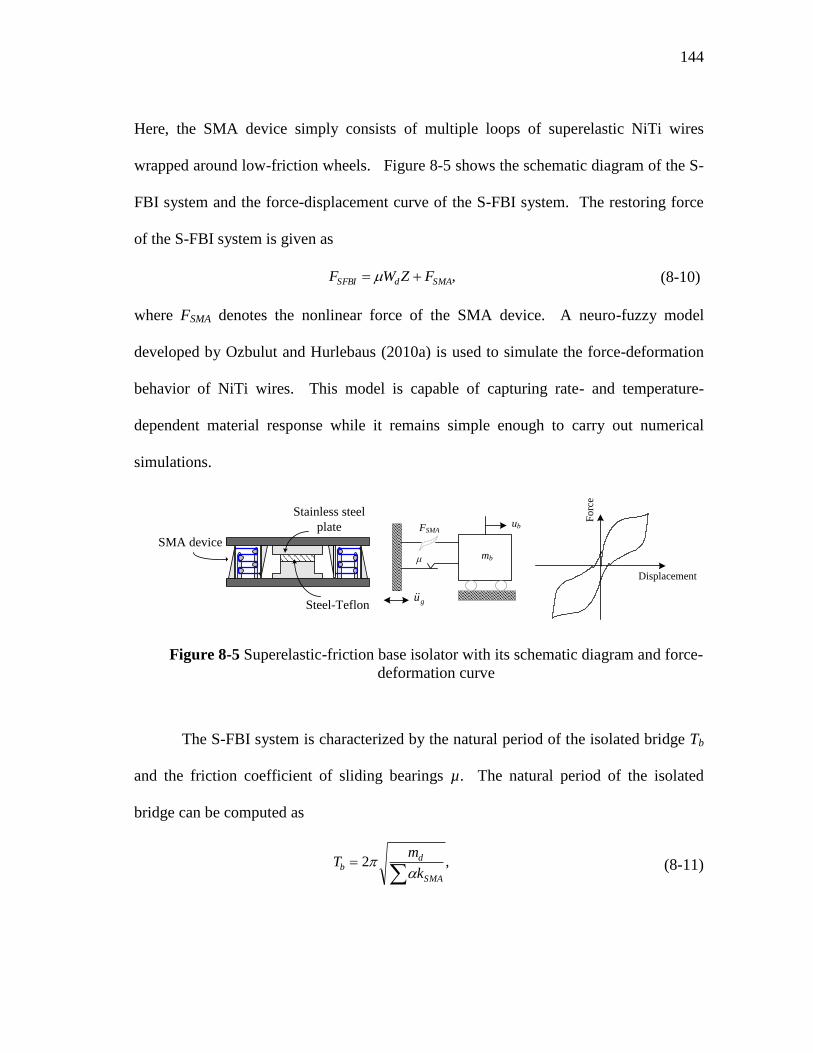
Figure 8-5 Superelastic-friction base isolator with its schematic diagram and force-
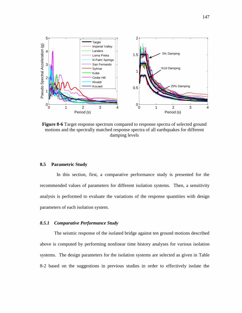
deformation curve ....................................................................................... 144
Figure 8-6 Target response spectrum compared to response spectra of selected
ground motions and the spectrally matched response spectra of all
earthquakes for different damping levels .................................................... 147
Figure 8-7 Peak deck drift for the various isolation systems subjected to near-field
earthquakes .................................................................................................. 149
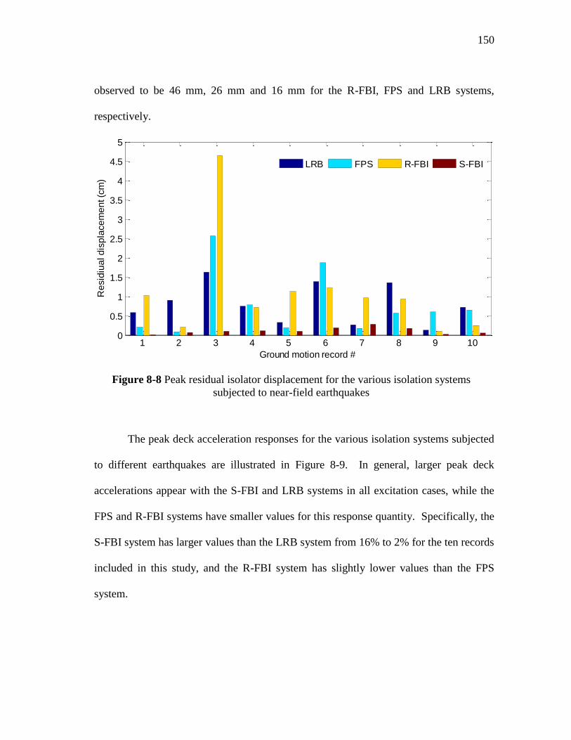
Figure 8-8 Peak residual isolator displacement for the various isolation systems
subjected to near-field earthquakes ............................................................. 150
Figure 8-9 Peak deck acceleration for the various isolation systems subjected to
near-field earthquakes ................................................................................. 151
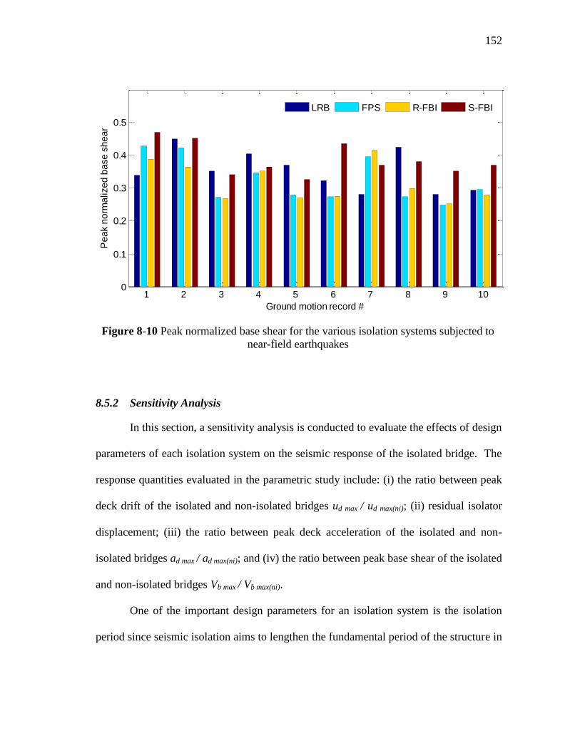
Figure 8-10 Peak normalized base shear for the various isolation systems subjected
to near-field earthquakes ............................................................................ 152
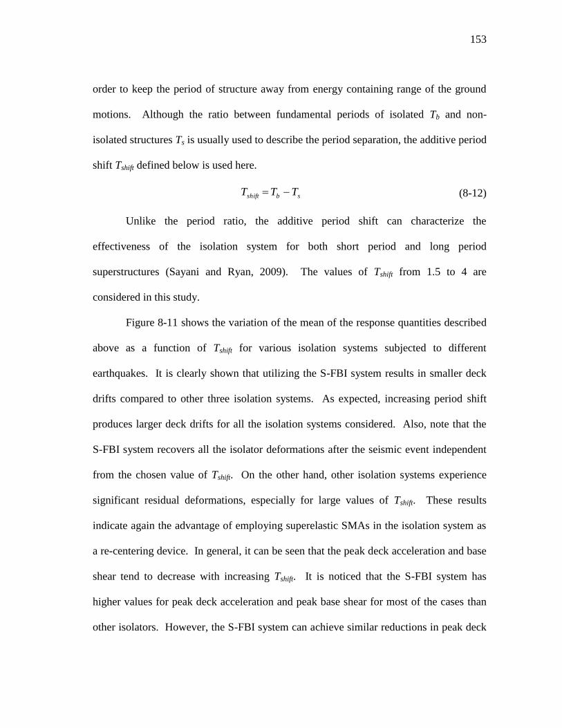
Figure 8-11 Variations of the mean response quantities with Tshift for various
isolation systems ......................................................................................... 154
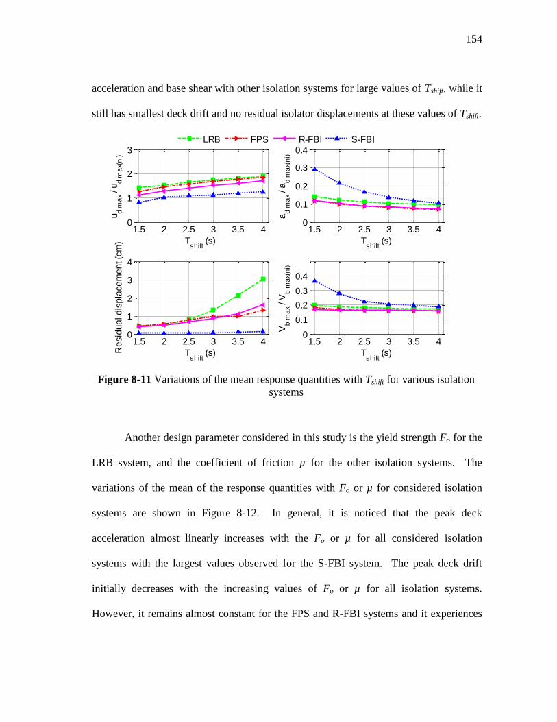
Figure 8-12 Variations of the mean response quantities with Fo or µ for various
isolation systems ......................................................................................... 155
Page 18
xvii
Page
Figure 9-1 Five-span continuous bridge and its model with sliding bearings and
SMA device ................................................................................................. 159
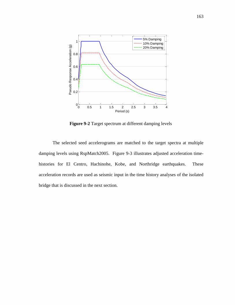
Figure 9-2 Target spectrum at different damping levels ............................................... 163
Figure 9-3 Spectrally matched acceleration time histories used in simulations............ 164
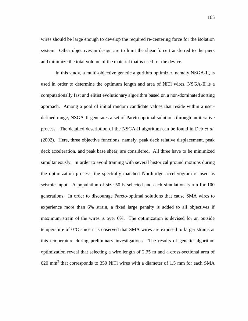
Figure 9-4 Maximum drifts of pier and deck at different temperatures ........................ 167
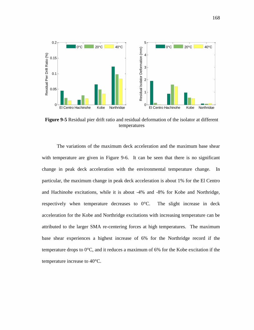
Figure 9-5 Residual pier drift ratio and residual deformation of the isolator at
different temperatures ................................................................................. 168
Figure 9-6 Maximum deck acceleration and maximum base shear at different
temperatures ................................................................................................ 169
Figure 9-7 Time histories of deck relative displacement and deck acceleration at
0°C and 40°C .............................................................................................. 170
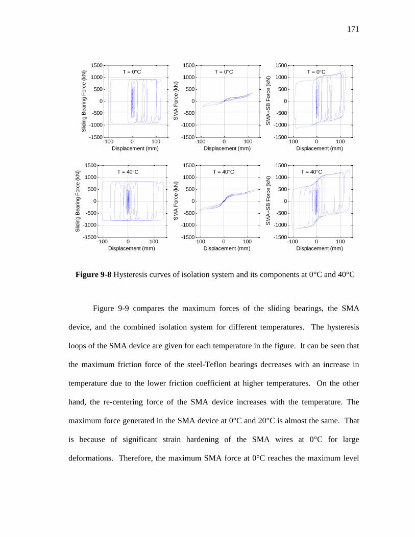
Figure 9-8 Hysteresis curves of isolation system and its components at 0°C and
40°C ............................................................................................................ 171
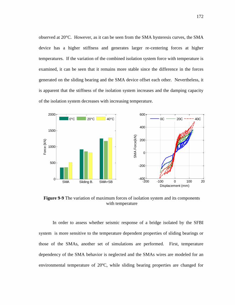
Figure 9-9 The variation of maximum forces of isolation system and its
components with temperature ..................................................................... 172
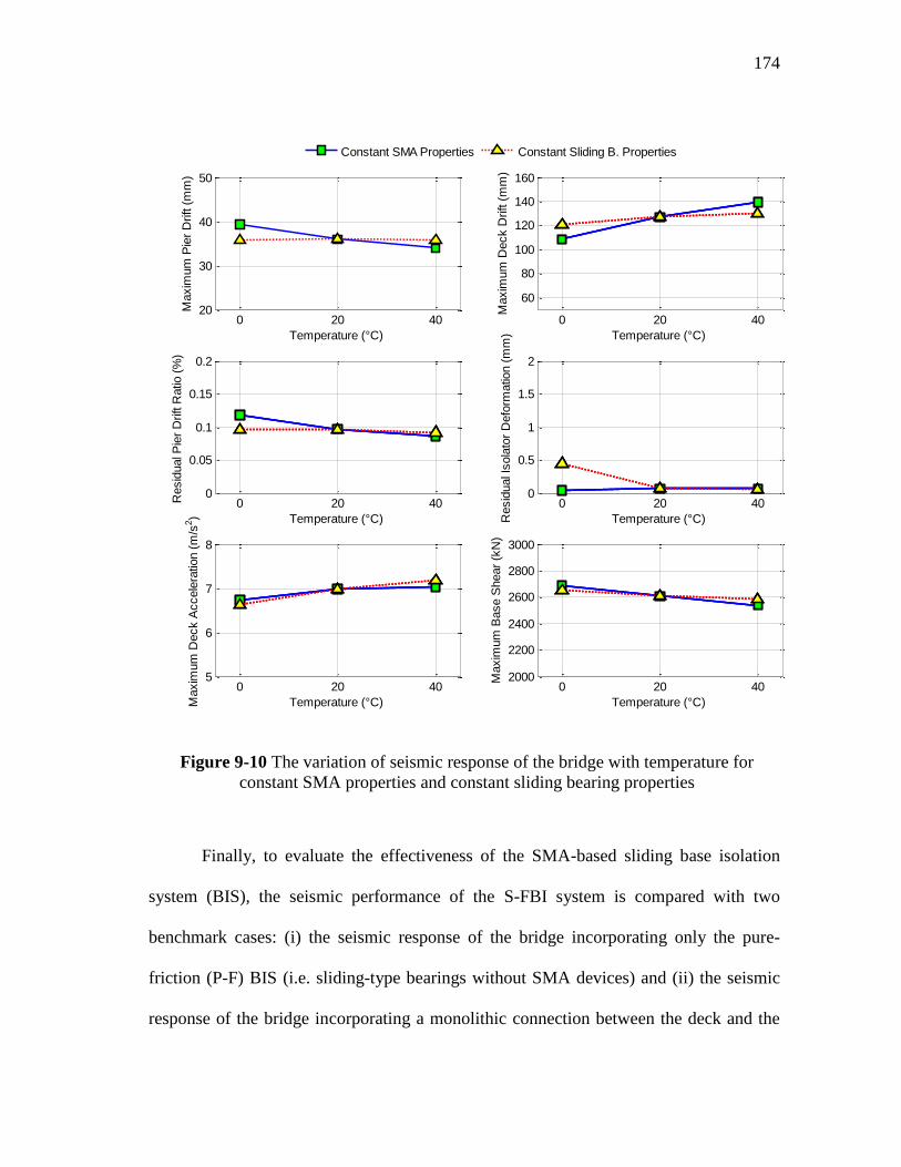
Figure 9-10 The variation of seismic response of the bridge with temperature for
constant SMA properties and constant sliding bearing properties ............. 174
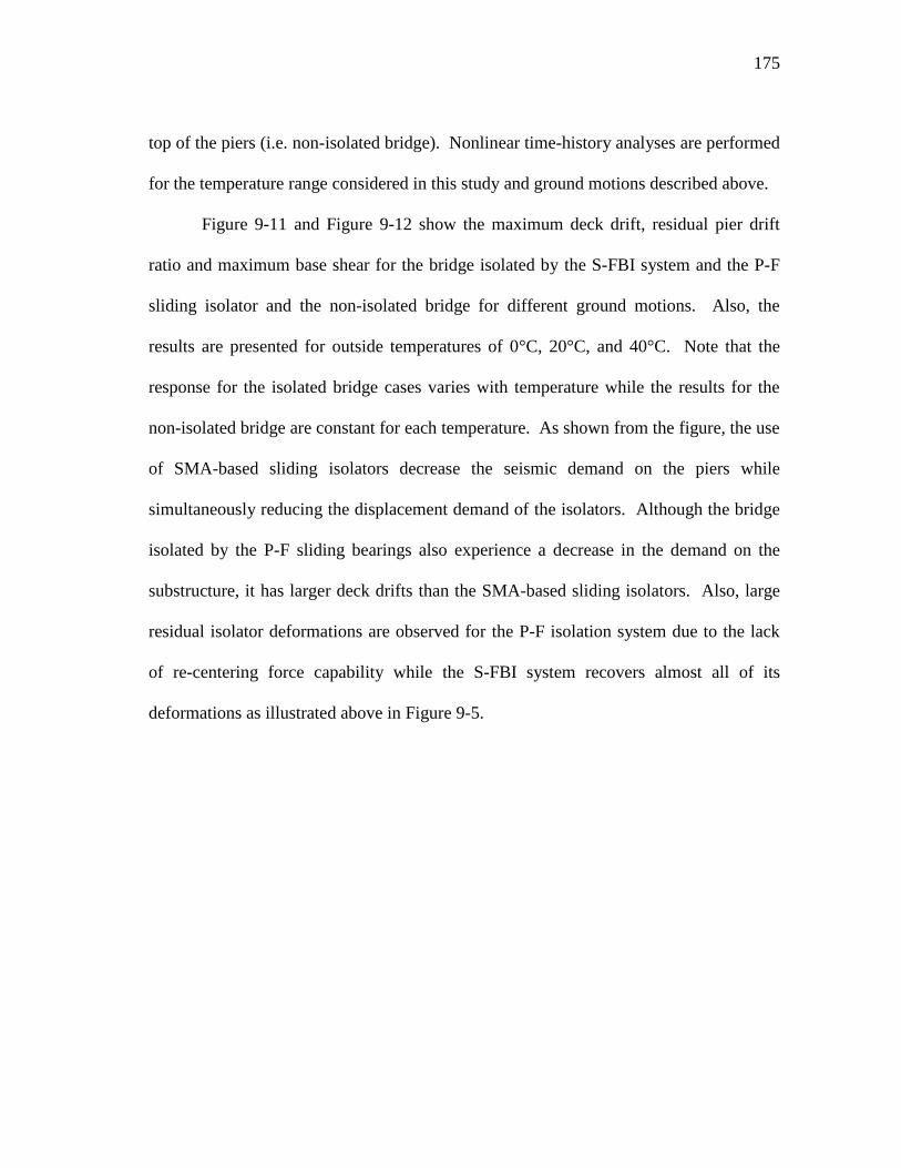
Figure 9-11 Seismic response comparison of different bridge configurations at
various temperatures for (a) El Centro and (b) Hachinohe earthquakes .... 176
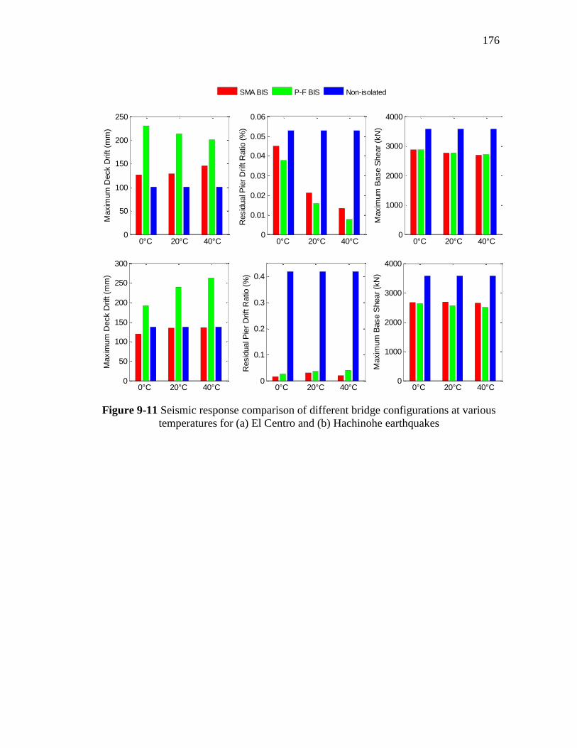
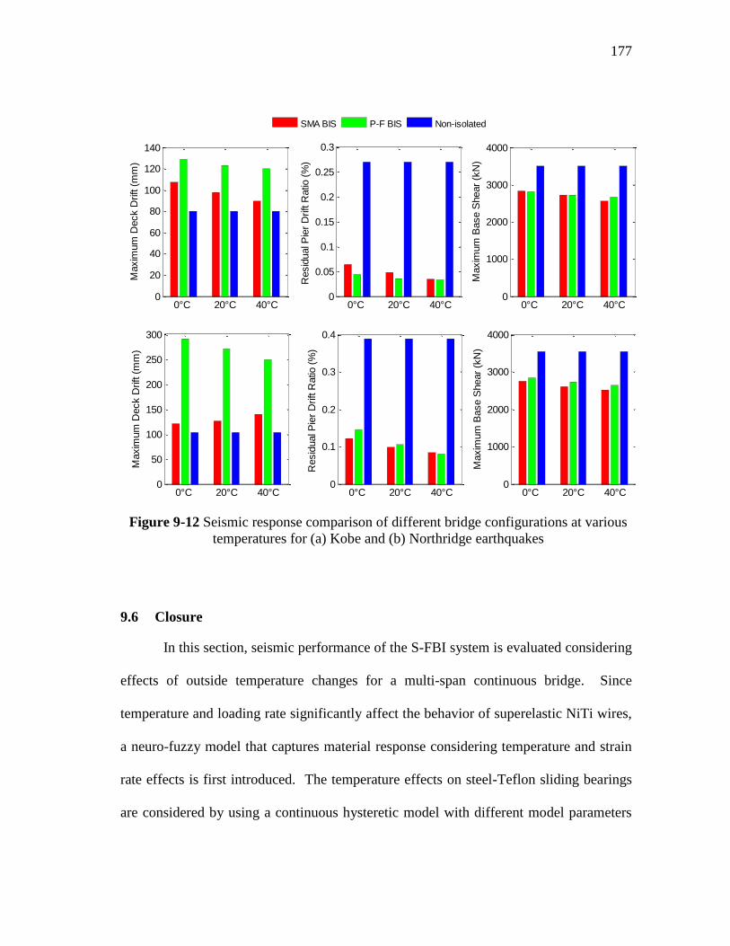
Figure 9-12 Seismic response comparison of different bridge configurations at
various temperatures for (a) Kobe and (b) Northridge earthquakes ........... 177
Page 19
xviii
LIST OF TABLES
Page
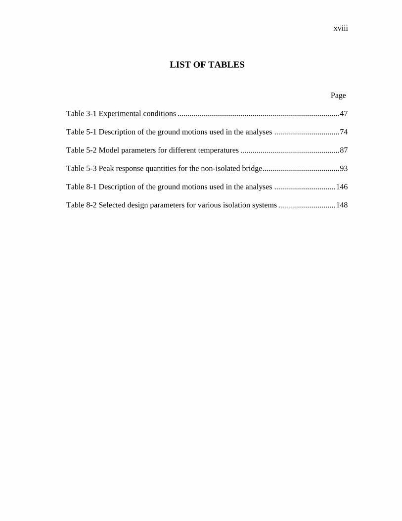
Table 3-1 Experimental conditions .................................................................................. 47
Table 5-1 Description of the ground motions used in the analyses ................................. 74
Table 5-2 Model parameters for different temperatures .................................................. 87
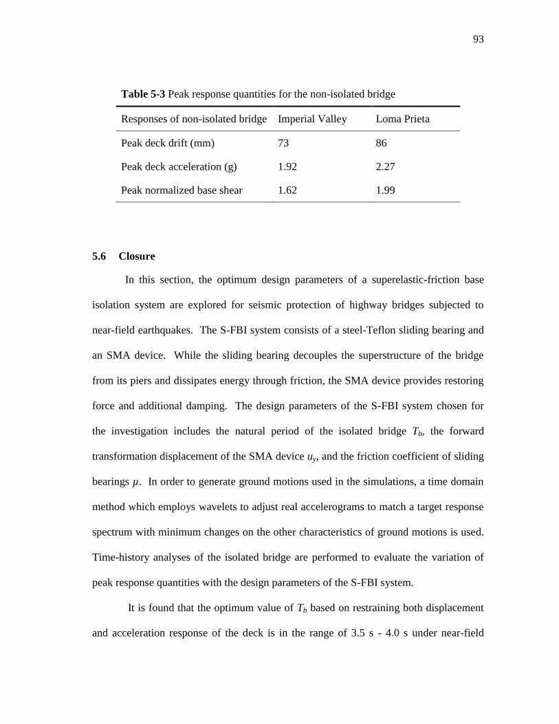
Table 5-3 Peak response quantities for the non-isolated bridge ....................................... 93
Table 8-1 Description of the ground motions used in the analyses ............................... 146
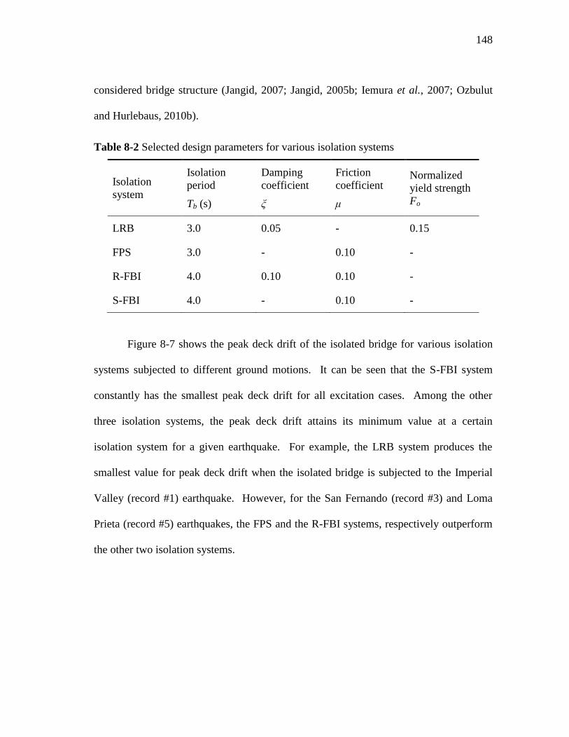
Table 8-2 Selected design parameters for various isolation systems ............................. 148
Page 20
xix
NOMENCLATURE
ABBREVIATIONS
AASHTO American Association of State Highway and Transportation
Officials
ANFIS Adaptive Neuro-Fuzzy Inference System
CFPR Carbon Fiber-Reinforced Polymer
ECC Engineering Cementitious Composites
FIS Fuzzy Inference System
FPS Friction Pendulum System
IBC International Building Code
LRB Lead Rubber Bearing
MANSIDE Memory Alloys for New Seismic Isolation and Energy
Dissipation Devices
MTS Material Testing System
NRB Natural Rubber Bearing
P-F Pure-Friction (isolation system)
PGA Peak Ground Acceleration
RC Reinforced Concrete
RHD Reusable Hysteretic Damper
R-FBI Resilient-Friction Base Isolator
S-FBI Superelastic-Friction Base Isolator
SMA Shape Memory Alloy
Page 21
xx
SRB SMA/rubber-based (isolation system)
SYMBOLS
ad max Peak deck acceleration of isolated bridge
ad max(ni) Peak deck acceleration of non-isolated bridge
Af Austenite finish temperature
Al Aluminum
As Austenite start temperature
ASMA Cross-sectional area of SMA wires
B Boron
Be Beryllium
C Carbon
c1 Viscous damping coefficient of piers
cb Viscous damping coefficient of bearing
Co Cobalt
Cu Copper
EA Absorbed energy
EH Irrecoverable hysteretic energy
EK Absolute kinetic energy
'
KE Relative kinetic energy
EI Absolute input energy
'
IE Relative input energy
Page 22
xxi
ES Elastic strain energy
ESMA Young‘s modulus of SMA wires
Eξ Damping energy
Fd Design force of SMA device
Fe Iron
Fo Normalized yield strength
Fy Yield strength
g Gravity
k1 Stiffness of piers
kb Initial stiffness of bearing
kSMA Initial lateral stiffness of SMA device
LSMA Length of SMA wires
m1 Mass of pier
m2 Mass of deck
Md Austenite stabilization temperature
Mf Martensite finish temperature
Mn Manganese
Ms Martensite start temperature
Nb Niobium
Ni Nickel
R Radius of the concave surface of FPS
Ta Tantalum
Page 23
xxii
Tb Natural period of the isolated bridge
Ti Titanium
Tshift Additive period shift
u1 Displacement of pier
u2 Displacement of deck
gu
Ground acceleration
ud Design displacement of SMA device
ud max Peak deck drift of the isolated bridge
ud max(ni) Peak deck drift of the non-isolated bridge
uy Yield displacement
Vb max Peak base shear of the isolated bridge
Vb max(ni) Peak base shear of the non-isolated bridge
Wd Weight of the deck
Zn Zinc
z Hysteretic dimensionless quantity
α Ratio of the post yielding to the elastic stiffness
εy Yield strain of SMA wire
μ Coefficient of friction
Page 24
1
1. INTRODUCTION
1.1 Problem Description
Bridges play an important role in the transportation network on which goods and
people are transported, and their failure will not only result in an interruption of this
basic need but also impede the relief and rescue efforts. In recent years, the damaging
effects of near-field motions on highway bridges have revealed the limitations of
conventional design methods and emphasized the need of innovative design strategies.
Numerous bridges were damaged or collapsed during the 1994 Northridge, 1995 Kobe,
1999 Duzce and 1999 Chi Chi earthquakes (Housner and Thiel, 1995; Bruneau, 1998;
Roussis et al., 2003; Hsu and Fu, 2004). In the most recent 2008 Winchuan earthquake,
many highway bridges were either severely damaged or completely collapsed in China,
leading to not only significant economic losses but also large loss of lives due to the
transportation supply disruption and the lack of access to medical care (Qiang et al.,
2009).
Seismic isolation has been the most commonly used method over the past years,
although numerous strategies have been proposed, to improve the response of bridge
structures during earthquakes (Ibrahim, 2008). Seismic isolation is essentially based on
the idea of decoupling the support of a structure from the horizontal motions of the
ground by placing flexible interfaces between the structure and its support. It reduces the
___________
This dissertation follows the style of Journal of Structural Engineering.
Page 25
2
lateral forces that act on the superstructure by shifting the fundamental period of the
structure away from the predominant period of the ground motion and providing
additional damping. A variety of devices including rubber isolation systems that
combine laminated rubber bearings and some mechanical dampers as well as sliding-
type isolation systems that filter out earthquake forces via the discontinuous sliding
interfaces have been developed and used for seismic isolation.
Although seismic isolation systems have been proven to be an effective method
of reducing seismic response of structures, the performance of base-isolated structures
against near-field earthquakes has been questioned in recent years (Jangid and Kelly,
2001; Shen et al., 2004; Liao et al., 2004). Near-field earthquakes are characterized by
long period and large velocity pulses in the velocity time history. Since the period of
these pulses usually coincides with the period of isolated structures, ground motions with
near-field characteristics amplify the seismic response of the isolation system. Another
characteristic of the near-field motions that adversely influences base isolation systems
is that the ground motion normal to the fault trace is richer in long-period spectral
components than that parallel to the fault. Isolation bearings experience large
deformations due to this normal component of the near-field motions (Deb, 2004). To
accommodate large isolator displacements, the size of the isolation device and the
required seismic gap significantly increases. Besides these requirements, the need for
flexible utility connections adds extra cost (Panchal and Jangid, 2008). Furthermore, if
an adequate seismic gap is not provided, undesirable pounding effects may occur.
Page 26
3
In order to reduce large displacement response of isolated bridge structures
during near-field earthquakes, several researchers have proposed the use of supplemental
dampers. Some studies are focused on the use of passive devices for additional energy
dissipation (Makris and Zhang, 2004; Soneji and Jangid, 2007; Dicleli, 2007), while a
considerable number of studies have explored the effectiveness of semi-active devices
for mitigating the response of isolated bridges (Erkus et al., 2002; Iemura and Pradono,
2005; Guo et al., 2009). However, a smart isolation system that can reduce the large
isolation level deformations that are observed during near-field excitations while still
offer the potential benefits of seismic isolation such as reductions in superstructure
acceleration response and base shear is still being pursued by researchers.
1.2 Scope of Research
Over the past decade, shape memory alloys have received considerable attention
as a smart material that can be employed in vibration control of civil structures
(DesRoches and Smith, 2004; Song et al., 2006). SMAs are a class of metallic alloys
that can recover their original shape after experiencing large strains. This study explores
the feasibility and effectiveness of SMA-based isolation systems in order to mitigate the
response of bridge structures against near-field ground motions. Seismic isolation
systems are typically rubber-based bearings or sliding-type bearings. Rubber isolation
bearings have considerable lateral flexibility and lengthen the natural period of the
structure in order to avoid resonance with the predominant frequency contents of the
ground motions, while sliding-type bearings provide discontinuous sliding interfaces to
Page 27
4
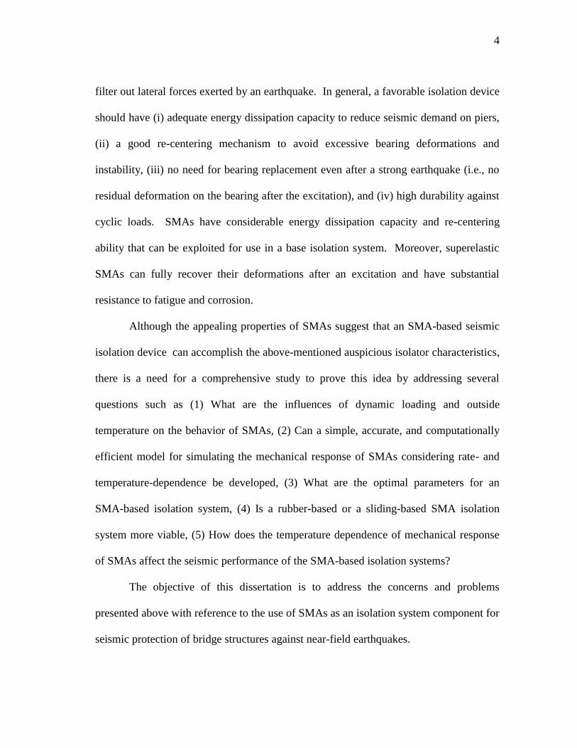
filter out lateral forces exerted by an earthquake. In general, a favorable isolation device
should have (i) adequate energy dissipation capacity to reduce seismic demand on piers,
(ii) a good re-centering mechanism to avoid excessive bearing deformations and
instability, (iii) no need for bearing replacement even after a strong earthquake (i.e., no
residual deformation on the bearing after the excitation), and (iv) high durability against
cyclic loads. SMAs have considerable energy dissipation capacity and re-centering
ability that can be exploited for use in a base isolation system. Moreover, superelastic
SMAs can fully recover their deformations after an excitation and have substantial
resistance to fatigue and corrosion.
Although the appealing properties of SMAs suggest that an SMA-based seismic
isolation device can accomplish the above-mentioned auspicious isolator characteristics,
there is a need for a comprehensive study to prove this idea by addressing several
questions such as (1) What are the influences of dynamic loading and outside
temperature on the behavior of SMAs, (2) Can a simple, accurate, and computationally
efficient model for simulating the mechanical response of SMAs considering rate- and
temperature-dependence be developed, (3) What are the optimal parameters for an
SMA-based isolation system, (4) Is a rubber-based or a sliding-based SMA isolation
system more viable, (5) How does the temperature dependence of mechanical response
of SMAs affect the seismic performance of the SMA-based isolation systems?
The objective of this dissertation is to address the concerns and problems
presented above with reference to the use of SMAs as an isolation system component for
seismic protection of bridge structures against near-field earthquakes.
Page 28
5
1.3 Organization of the Dissertation
This dissertation is organized into the following sections:
Section 1 presents the description of research problem and the scope of the
research.
Section 2 provides a concise overview of mechanical properties of shape memory
alloys and modeling techniques for SMAs. Also, a comprehensive literature review is
presented for passive vibration control applications using SMAs.
Section 3 presents tensile tests conducted to evaluate the effects of temperature,
strain rate, and strain amplitude on mechanical behavior of superelastic NiTi wires.
Section 4 discusses the neuro-fuzzy modeling of temperature- and rate-
dependent behavior of superelastic NiTi SMAs.
Section 5 investigates the optimum design parameters of a superelastic-friction
base isolator (S-FBI) that consists of a steel-Teflon sliding bearing and a superelastic
SMA device for seismic protection of bridges subjected to near-field earthquakes.
Section 6 explores the effectiveness of an SMA/rubber-based (SRB) isolation
system that consists of a laminated rubber bearing and an SMA device for protecting
highway bridges against near-field earthquakes.
Section 7 compares the performances of the superelastic-friction base isolator
and the SMA/rubber-based isolation system using energy-based concepts.
Section 8 presents a comparative study of the performances of various isolation
systems such as lead rubber bearings, friction pendulum system, resilient-friction base
Page 29
6
isolators and the superelastic-friction base isolators for a multi-span continuous bridge
under near-field ground motions.
Section 9 explores the effects of temperature on the performance of the
superelastic-friction base isolator at length.
Section 10 presents conclusions along with recommendations for the use of
SMAs as a seismic isolation component based on the findings of this study.
Page 30
7
2. SHAPE MEMORY ALLOYS: AN OVERVIEW
2.1 Introduction to Shape Memory Alloys
The term smart materials usually refers to materials that have unique and
interesting characteristics and can be employed in conventional structural design to
improve performance of the structure. Shape memory alloys are a smart class of metals
that exhibit several extraordinary properties. SMAs have two main phases which have
different crystal structure. One is called martensite that is stable at low temperatures and
high stresses and the other is called austenite that is stable at high temperatures and low
stresses. Austenite, also named as parent phase, generally has a cubic crystal structure
while martensite has a less-ordered crystal structure. Martensite can exist in two forms
depending on crystal orientation direction: twinned (self-accommodated) martensite or
detwinned martensite. Figure 2-1 shows schematic representation of different phases of
shape memory alloy materials. The key characteristic of SMAs is a result of reversible
phase transformations between martensite and austenite phases. These solid-to-solid
phase transformations, called martensitic transformations, occur by shear lattice
distortion with no diffusive process involved. The transformations can be temperature-
induced (shape memory effect) or stress-induced (superelasticity).
Page 31
8
Twinned
martensiteDetwinned
martensite Austenite
Figure 2-1 Different phases of shape memory alloys
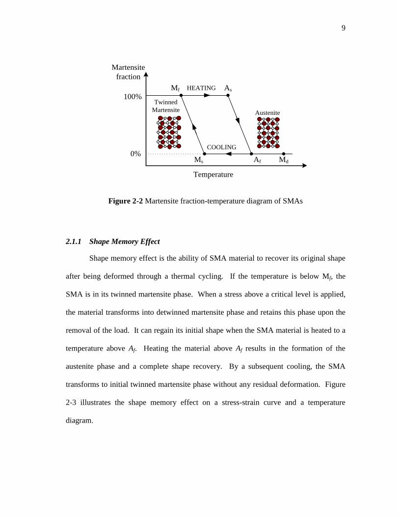
Figure 2-2 illustrates the martensite fraction in an SMA material as a function of
temperature in the absence of applied stress. There are four characteristic temperatures
at which phase transformations occur: (1) the austenite start temperature As, where the
material starts to transform from twinned martensite to austenite, (2) austenite finish
temperature Af, where the material is completely transformed to austenite, (3) martensite
start temperature Ms, where austenite begins to transform into twinned martensite, (4)
martensite finish temperature Mf, where the transformation to martensite is completed.
Note that all of these transformation temperatures would increase with applied stress.
Page 32
9
Af
As
Ms
Mf
Temperature
Martensite
fraction
100%
0%Md
Austenite
Twinned
Martensite
HEATING
COOLING
Figure 2-2 Martensite fraction-temperature diagram of SMAs
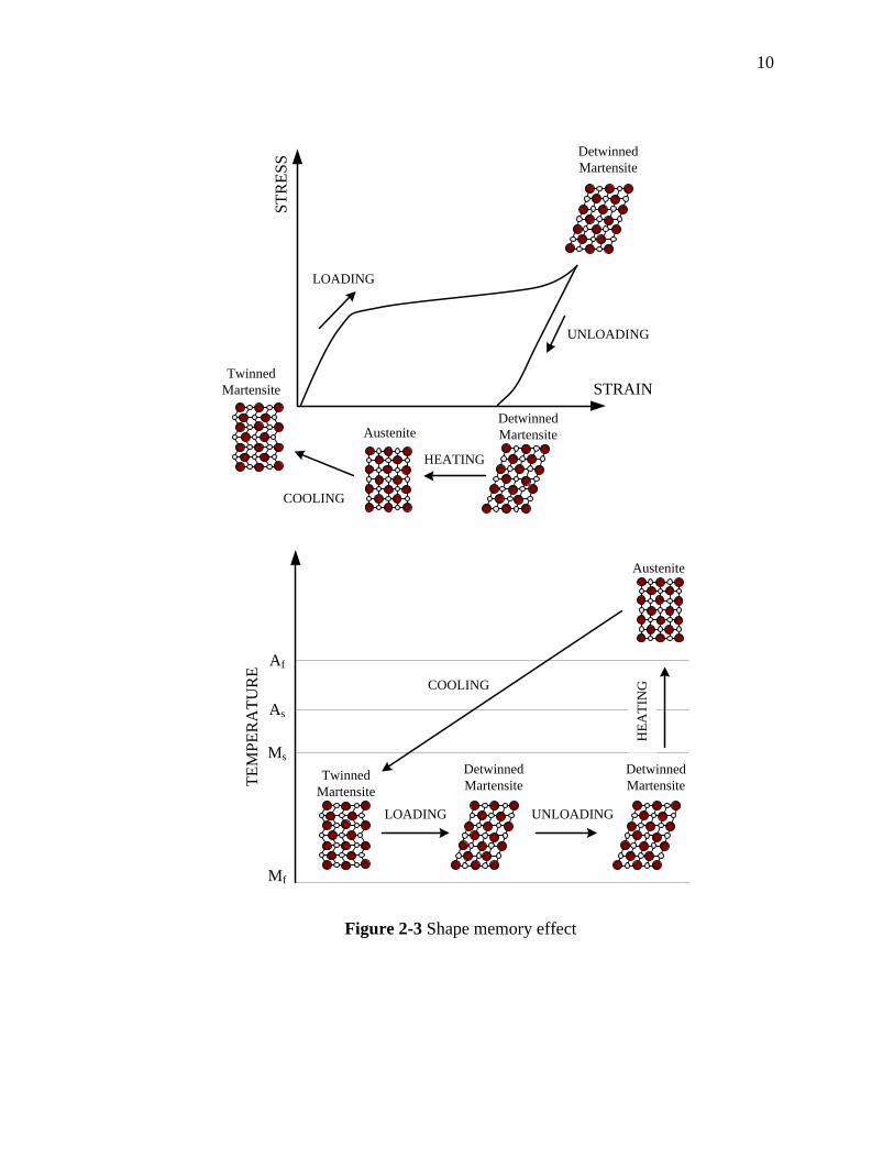
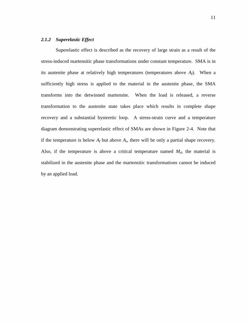
2.1.1 Shape Memory Effect
Shape memory effect is the ability of SMA material to recover its original shape
after being deformed through a thermal cycling. If the temperature is below Mf, the
SMA is in its twinned martensite phase. When a stress above a critical level is applied,
the material transforms into detwinned martensite phase and retains this phase upon the
removal of the load. It can regain its initial shape when the SMA material is heated to a
temperature above Af. Heating the material above Af results in the formation of the
austenite phase and a complete shape recovery. By a subsequent cooling, the SMA
transforms to initial twinned martensite phase without any residual deformation. Figure
2-3 illustrates the shape memory effect on a stress-strain curve and a temperature
diagram.
Page 33
10
ST
RE
SS
Detwinned
Martensite
Twinned
Martensite
HEATING
STRAIN
TE
MP
ER
AT
UR
E
Twinned
Martensite
Detwinned
Martensite
Austenite
Ms
Mf
As
Af
LOADING
HE
AT
INGCOOLING
Detwinned
Martensite
UNLOADING
Detwinned
MartensiteAustenite
COOLING
LOADING
UNLOADING
Figure 2-3 Shape memory effect
Page 34
11
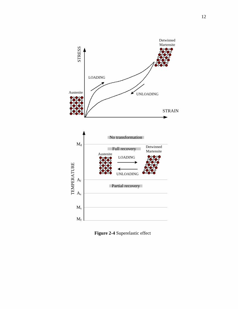
2.1.2 Superelastic Effect
Superelastic effect is described as the recovery of large strain as a result of the
stress-induced martensitic phase transformations under constant temperature. SMA is in
its austenite phase at relatively high temperatures (temperatures above Af). When a
sufficiently high stress is applied to the material in the austenite phase, the SMA
transforms into the detwinned martensite. When the load is released, a reverse
transformation to the austenite state takes place which results in complete shape
recovery and a substantial hysteretic loop. A stress-strain curve and a temperature
diagram demonstrating superelastic effect of SMAs are shown in Figure 2-4. Note that
if the temperature is below Af but above As, there will be only a partial shape recovery.
Also, if the temperature is above a critical temperature named Md, the material is
stabilized in the austenite phase and the martensitic transformations cannot be induced
by an applied load.
Page 35
12
0 1 2 3 4 5
0
100
200
300
400
500
600
Austenite
Detwinned
Martensite
TE
MP
ER
AT
UR
E
Austenite
Ms
Mf
As
Af
LOADING
UNLOADING
Detwinned
Martensite
Md
Partial recovery
Full recovery
No transformation
ST
RE
SS
STRAIN
LOADING
UNLOADING
Figure 2-4 Superelastic effect
Page 36
13
2.1.3 Commonly-used Shape Memory Alloys
Since the discovery of nickel-titanium (NiTi) in 1963, a large number of alloys
have been investigated for shape memory behavior. However, two alloy systems, NiTi-
based alloys and copper (Cu)-based alloys, have been mostly used in commercial
applications in the past decades. Iron-based alloys have also attracted the interest of
researchers in recent years.
2.1.3.1 NiTi-based alloys
Among various SMA compositions, the NiTi alloy has been the most widely
studied and has become the most important material for commercial applications. This
binary system is based on an almost equiatomic compound of nickel and titanium.
Increasing the nickel composition above 50 atomic percentage (at.%) decreases the
transformation temperature. Hence, the range of phase transformation temperatures can
be adjusted by altering the composition of the alloys. The NiTi can achieve fully
recoverable strains up to 8% and can be obtained in various forms such as wires, bars,
tubes and plates. One of the important characteristics of the NiTi alloy is its excellent
corrosion resistance. This feature of NiTi alloys together with their biocompatibility
aspects has lead to the use of NiTi in various medical applications.
The addition of a third metal to NiTi to compose a ternary can result in desirable
properties for specific applications. For example, NiTiCu has lower hysteresis
associated with phase transformations, which makes them a better choice for actuator
applications. On the other hand, the addition of Niobium (Nb) to the NiTi results in
wider thermal hysteresis. The alloy NiTiNb shows minimal response to large
Page 37
14
temperature changes and is preferred for coupling applications. It is also possible to
obtain SMAs for applications operating at high temperatures by adding a third element
such as palladium, platinum, hafnium and gold to the NiTi. In this way, transformation
temperatures can be shifted anywhere in the range of 100-800 °C (Lagoudas, 2008).
2.1.3.2 Copper-based alloys
The copper-based alloys have the advantage that they are composed of relatively
cheap materials and it is easier to machine them. However, because of the larger
demand for NiTi alloys from industry, especially for biomedical devices, the price of the
NiTi has decreased considerably over the past decade. Also, the recoverable strains for
Cu-based alloys are limited to 2-4% strain levels and they have a long term aging
problem at room temperatures due to martensite stabilization. The main Cu-based alloys
are based on the binary alloys CuAl and CuZn. Among the commercially available Cu-
based alloys, CuZnAl has the largest ductility whereas CuZnNi is less sensitive to aging
effect and stabilization. The transformation temperatures of these alloys can be altered
by varying the aluminum or nickel content. Although the transformation temperatures of
NiTi alloys can also be adjusted by alloying and thermomechanical treatments, Cu-based
alloys tend to have somewhat higher temperature range of transformation. For example,
CuAlBe alloy exhibits superelastic behavior at a temperature range of -65 °C to 180 °C,
which make them attractive for outdoor seismic application in cold regions. Recently,
several researches investigated CuAlMn-based SMAs for enhanced ductile behavior and
shape memory properties (Sutou et al., 2008).
Page 38
15
2.1.3.3 Iron-based alloys
As an alternative to NiTi-based alloys and copper-based alloys, ferrous SMAs
such as FeMnSi, FeNiC and FeNiCoTi have been developed due to their lower cost.
However, a ferrous alloy that exhibit superelastic effect at room temperature was not
available until most recently. Tanaka et al. (2010) obtained a ferrous alloy showing a
superelastic strain up to 15% at room temperature. The composition of the alloy is Fe-
28Ni-17Co-11.5Al-2.5Ta-0.05B at.%, and the alloy is named as NCATB. The alloy has
a tensile strength over 1 GPa. Also, austenite finish temperature Af of the NCATB is -62
°C, which indicates a superelastic SMA device made of NCATB can be used safely in
cold regions for outdoor seismic applications. Once the NCATB alloy is
commercialized, the unique characteristics of the alloy such as high strength, large
superelastic strain and high damping capacity might be exploited in various applications.
2.2 Mechanical Characteristics of Shape Memory Alloys
Since most of the seismic applications of SMAs rely on the superelastic effect of
the SMAs, the mechanical properties of the superelastic SMAs are discussed in this
section. The sensitivity of these properties to various factors such as temperature, strain
rate, cyclic loading, and thermomechanical treatment is also examined. The superelastic
SMAs that are considered for civil engineering applications includes the NiTi alloy and
the Cu-based alloys. The mechanical characteristics of these alloys are discussed
separately below.
Page 39
16
2.2.1 Characteristics of NiTi Alloy
NiTi shape memory alloys have appealing mechanical characteristics such as
considerable energy dissipation capacity, excellent re-centering ability, high strength,
good fatigue resistance and high corrosion resistance. However, there are a number of
parameters that influence the mechanical properties of the NiTi SMAs. Therefore, a
complete understanding of the mechanical behavior of the NiTi is required before
employing it in seismic applications. Many researchers have conducted experiments to
investigate the mechanical characteristics of superelastic NiTi SMAs. The following
discussion outlines the effects of cyclic loading, strain-rate and temperature on the
behavior of the NiTi SMA.
2.2.1.1 Cycling loading
Due to the cyclic nature of the seismic loads, it is important to characterize the
behavior of SMAs under repeated loading conditions. Some researchers have studied
the effect of cyclic loading on NiTi wires with a diameter of 1-2 mm (Wolons et al.,
1998; Dolce and Cardone, 2001; Gall et al., 2001; Tamai and Kitagawa, 2002;
DesRoches et al., 2004; Malecot et al., 2006). They found that there is a considerable
decrease in forward phase transformation stress level with the number of loading cycles.
Specifically, the greatest variation was noted between the first and second cycle. The
reason for this reduction in forward transformation stress resides in small levels of
localized slip that assist the forward transformation (DesRoches et al., 2004). No
significant variation or only a slight decrease was observed in the reverse transformation
stress. Therefore, hysteresis loop area, i.e. the dissipated energy reduces with increasing
Page 40
17
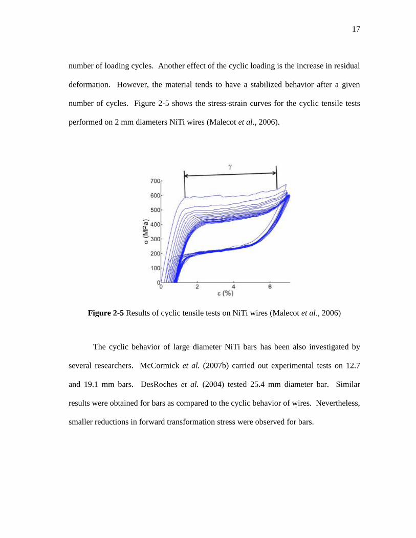
number of loading cycles. Another effect of the cyclic loading is the increase in residual
deformation. However, the material tends to have a stabilized behavior after a given
number of cycles. Figure 2-5 shows the stress-strain curves for the cyclic tensile tests
performed on 2 mm diameters NiTi wires (Malecot et al., 2006).
Figure 2-5 Results of cyclic tensile tests on NiTi wires (Malecot et al., 2006)
The cyclic behavior of large diameter NiTi bars has been also investigated by
several researchers. McCormick et al. (2007b) carried out experimental tests on 12.7
and 19.1 mm bars. DesRoches et al. (2004) tested 25.4 mm diameter bar. Similar
results were obtained for bars as compared to the cyclic behavior of wires. Nevertheless,
smaller reductions in forward transformation stress were observed for bars.
Page 41
18
2.2.1.2 Strain rate effects
Although martensitic phase transformations are time-independent phenomena,
experimental tests conducted at different loading rates have revealed that the strain rate
has a significant influence on the mechanical behavior of NiTi shape memory alloys.
The reason of the rate-dependent behavior is complex coupling between stress,
temperature and rate of heat generation during stress induced phase transformations
(Azadi et al, 2006). During the forward phase transformations, the material releases
energy in the form of heat, while it absorbs energy in the case of unloading. The
material may not have enough time to transfer latent heat to the environment during
loading with high strain rates. As a result, the temperature of the material changes and
this, in turn, alters the shape of the hysteresis loops and the transformation stresses (Wu
et al., 1996).
In the past studies, different conclusions were made about the effect of loading
rate on the transformation stresses and the energy dissipated. Wolons et al. (1998) and
Ren et al. (2007) reported an increase in the reverse transformation stress without a
significant change in the forward transformation stress and a decrease in the energy
dissipated with the increased strain rates. Dolce and Cardone (2001) and DesRoches et
al. (2004) noticed an increase in both forward and reverse transformation stresses with
increasing strain rates. Since smaller increases were observed in the forward
transformation stress, a reduction in the energy dissipated was reported. On the other
hand, Tobushi et al. (1998) observed a decrease in the reverse transformation stress and
an increase in the forward transformation stress, which resulted in larger energy
Page 42
19
dissipation for higher strain rates. Dayananda and Rao (2008) found that hysteresis loop
shifts upward and the energy dissipated increases with increase in strain rates. Soul et
al. (2010) reported that the dissipated energy slightly increases for a low frequency
region (for frequencies less than 0.05 Hz), whereas it considerably decreases for a high
frequency region (for a frequency range of 0.05 Hz -3 Hz).
The inconsistency in the findings of the previous studies about the strain rate
effects on the superelastic behavior of NiTi SMAs can be attributed to factors such as
using materials with different composition, testing at various ranges of strain rates, and
experimental conditions. Since the SMA material employed in seismic applications will
be subjected to dynamic effects, it is important to evaluate the effect of strain rate on the
material used before actual application.
2.2.1.3 Temperature effects
Since phase transformations of SMAs are not only dependent on mechanical
loading but also on temperature, change in the temperature significantly affects
superelastic behavior of NiTi wires. Note that it is not only the testing temperature that
influence the behavior but also its position with respect to transformation temperatures.
A number of experimental studies have been conducted to investigate the effects of
temperature on superelastic SMAs (Piedboeuf et al., 1998; Dolce and Cardone, 2001;
Chen and Song, 2006; Churchill et al., 2009). It was reported that the critical stress that
initiates the phase transformation noticeably changes with temperature. In particular, an
increase in temperature corresponds to a linear increase in transformation stress. Also, it
was found that the equivalent viscous damping linearly decreases with an increase in the
Page 43
20
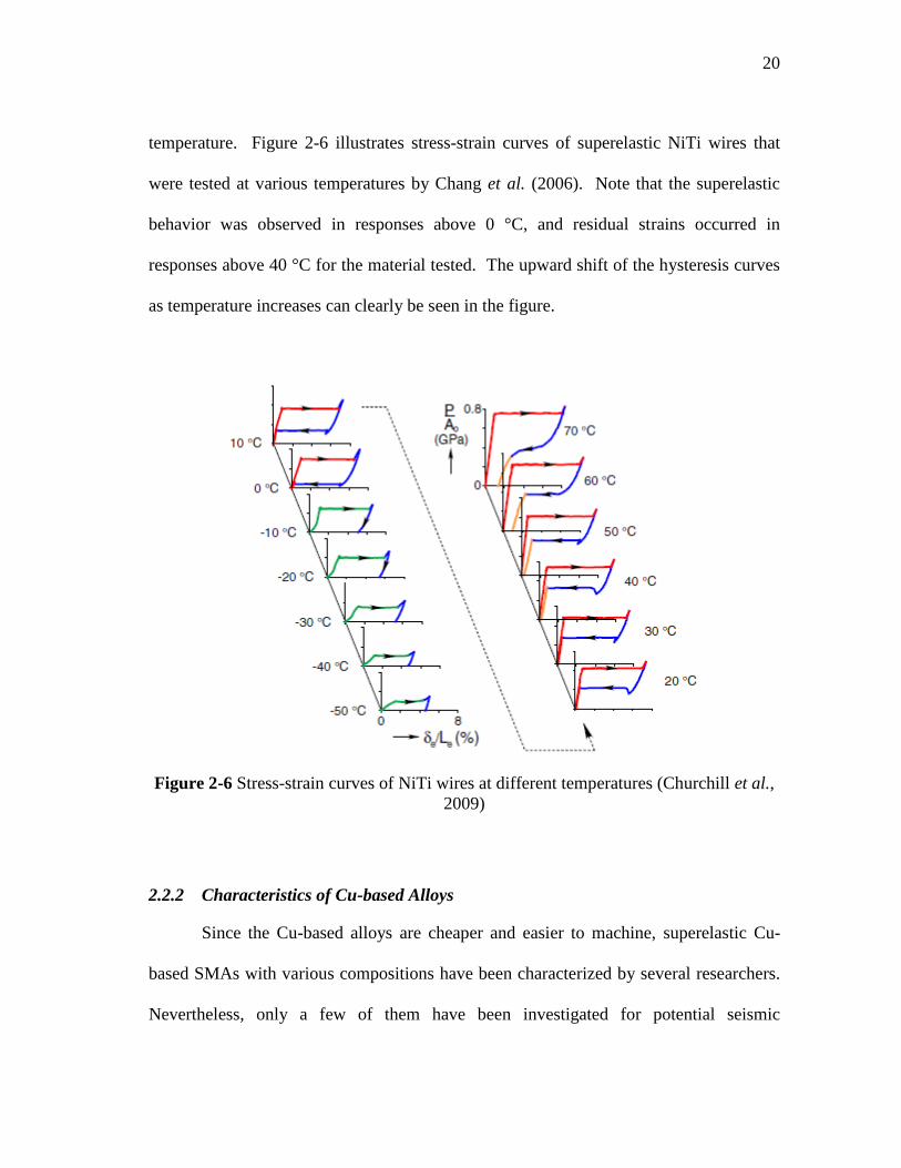
temperature. Figure 2-6 illustrates stress-strain curves of superelastic NiTi wires that
were tested at various temperatures by Chang et al. (2006). Note that the superelastic
behavior was observed in responses above 0 °C, and residual strains occurred in
responses above 40 °C for the material tested. The upward shift of the hysteresis curves
as temperature increases can clearly be seen in the figure.
Figure 2-6 Stress-strain curves of NiTi wires at different temperatures (Churchill et al.,
2009)
2.2.2 Characteristics of Cu-based Alloys
Since the Cu-based alloys are cheaper and easier to machine, superelastic Cu-
based SMAs with various compositions have been characterized by several researchers.
Nevertheless, only a few of them have been investigated for potential seismic
Page 44
21
applications. Among them, CuZnAlNi shape memory alloy bars were explored by
Moroni et al. (2002) for their use as energy dissipation device. They conducted cyclic
tests under tension-compression loading and evaluated their damping properties.
However, the CuAlBe alloy has been the most commonly considered Cu-based SMA for
seismic applications. The effects of cycling loading, strain rate, temperature and grain
size on mechanical properties of the superelastic CuAlBe alloy are discussed below.
2.2.2.1 Cycling loading
The effect of cyclic loading on mechanical response of the CuAlBe wires has
been studied by a number of researchers (Casciati and Faravelli, 2004; Montecinos et al.,
2006; Ozbulut et al., 2007; Zhang et al., 2008; Torra et al., 2009). It was found that
there is a decrease in forward transformation stress and hysteresis loop area with
increasing number of loading cycles. However, it was reported that a stable behavior
can be obtained after the first 10 load cycles. Also, no remnant strain occurred after
many series of loading cycles. In a most recent study, Casciati and Marzi (2010)
conducted an exhaustive set of experimental tests to investigate the fatigue lifetime of
the CuAlBe SMAs for seismic applications. They concluded that the fatigue life of the
CuAlBe is strongly dependent to the thermo-mechanical history of the material and
strain amplitude. The fatigue life of the specimens subjected to a preliminary thermo-
mechanical treatment was found to be satisfactory for strain amplitudes below 3%.
Also, a reduced fatigue life was recorded for the specimens tested at higher
temperatures.
Page 45
22
2.2.2.2 Strain rate effects
Studies that explore the effects of strain rate on mechanical properties of CuAlBe
SMAs have remained few in number. Among them, Malecot et al. (2006) performed
tensile tests at four different strain rates, Araya et al. (2008) carried out cyclic tests at
three different frequencies and Zhang et al. (2008) tested the CuAlBe wires at two
different loading rates. No significant influence of strain rate on the shape of hysteresis
curve and energy dissipation capacity was reported in the findings of these studies.
2.2.2.3 Temperature effects
Several studies have been conducted to evaluate the influence of temperature on
the mechanical response of the CuAlBe alloys (Torra et al., 2004; Araya et al., 2008;
Casciati and van der Eijk, 2008). In such a study, Ozbulut et al. (2007) carried out
tensile tests on the CuAlBe wires at 0 °C, 25 °C, and 50 °C. They found that modulus of
elasticity, secant stiffness and phase transformation stresses increase with increasing
temperature. Also, a decrease in equivalent viscous damping was observed as the
temperature increases. Zhang et al. (2008) investigated the behavior of the CuAlBe
SMAs at cold temperatures. In particular, they compared the behavior of the CuAlBe
wires tested at -50 °C, -25 °C, 0 °C and 23 °C. They reported a slight decrease in
equivalent viscous damping and an increase in forward transformation stress for higher
temperatures. No clear pattern for the variation of elasticity modulus with temperature
was observed. Figure 2-7 illustrates the dependence of mechanical behavior of the
CuAlBe wires on temperature.
Page 46
23
Figure 2-7 Stress-strain curves of CuAlBe wires at different temperatures (Zhang et al.,
2008)
2.2.2.4 Grain size effects
The size, shape, and crystallographic orientation of grains have a considerable
influence on the superelastic behavior of Cu-based SMAs. The grain size in Cu-based
SMAs is of larger magnitude than that for NiTi alloys. Therefore, elastic stress
concentrations on grain boundaries are easily relaxed by plastic deformation in NiTi
whereas elastic stress concentrations easily occur at grain boundaries of Cu-based alloys.
This is why the mechanical behavior of NiTi alloy is only slightly influenced by grain
size and orientation. On the contrary, large grain sizes cause intergranular brittle
fractures in Cu-based SMAs due to stress concentrations on grain boundaries (Brailovski
et al., 2003).
Araya et al. (2008) investigated grain size effects on the mechanical behavior of
the CuAlBe SMA wires. They found that the maximum stress and forward
Page 47
24
transformation stress increase as the grain size decreases. Also, an increase in equivalent
viscous damping was present with increased grain size. Similarly, Boroschek et al.
(2007) found that a coarse grain size leads to smaller secant stiffness and higher energy
loss for the CuAlBe alloys. However, very large grain sizes cause brittle fracture and
need to be avoided.
2.3 Modeling of Shape Memory Alloys
In order to explore all potential applications of SMAs, a reliable model that
describes highly complex behavior of the material has been pursued by many
researchers. SMA models have been developed by either following a microscopic or a
macroscopic approach. The first approach actually aims to describe phenomena in either
microscopic or mesoscopic level. At microscopic level, models employ continuum
mechanics to relate deformation, strain, and stress at particular points for a small
material volume. The models that describe the behavior of SMA at mesoscopic level
also use continuum mechanics as main description tool but combine it with multiscale
modeling. The microscopic approach has been studied in the work of many researchers
such as Sun and Hwang (1993), Goo and Lexcellent (1997), Levitas et al. (1998),
Patoor et al. (1998), Hall and Govindjee (2002).
Macroscopic models attempt to capture the SMA response at the macroscopic
level using phenomology. Some of these models rely heavily on thermodynamic
principles, while others are developed by setting material constants of a model to match
experimental data. A large number of macroscopic models have been proposed to
Page 48
25
capture mechanical response of SMA due to their simplicity and relative accuracy (Boyd
and Lagoudas, 1996; Liang and Rogers, 1990; Auricchio and Lubliner, 1997; Auricchio,
2001; Ikeda et al., 2004). This section does not aim to provide an exhaustive review of
all models that describe constitutive behavior of SMAs in the existing literature. Rather,
it introduces some of the constitutive models of superelastic SMAs that have been
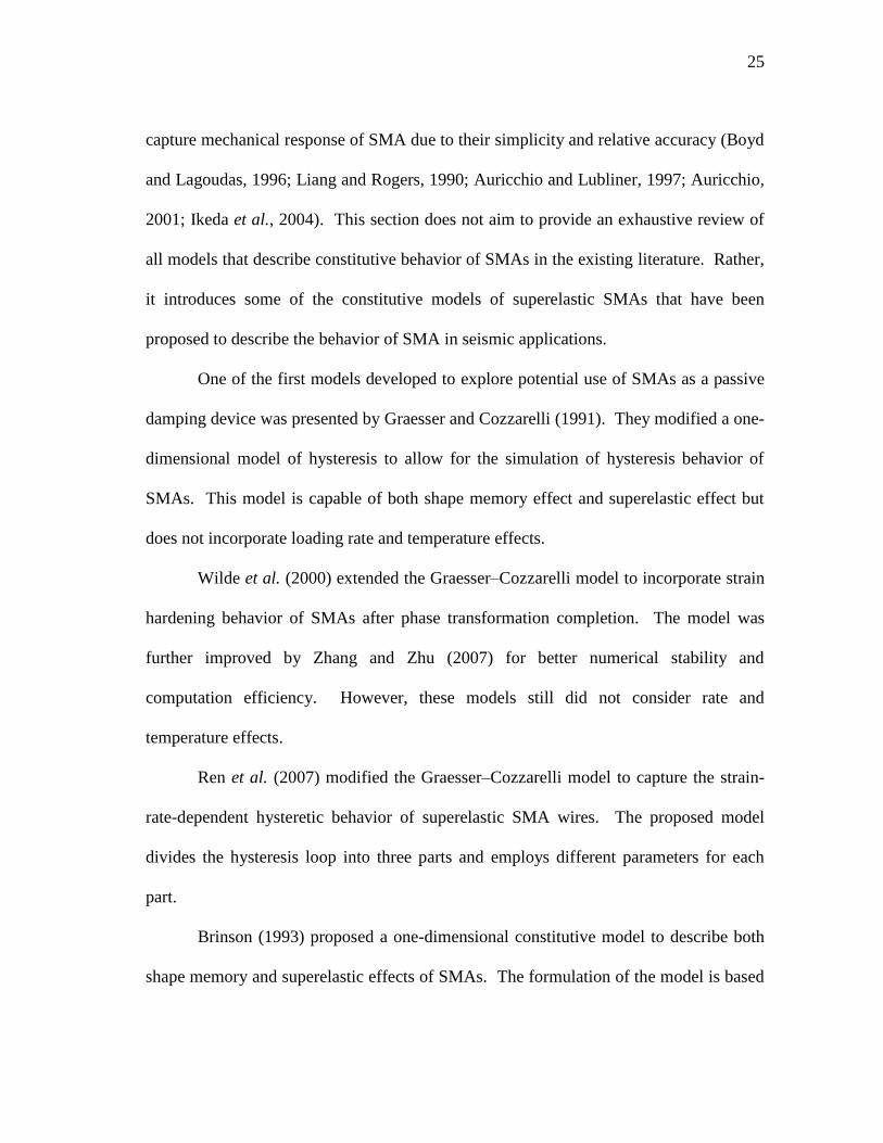
proposed to describe the behavior of SMA in seismic applications.
One of the first models developed to explore potential use of SMAs as a passive
damping device was presented by Graesser and Cozzarelli (1991). They modified a one-
dimensional model of hysteresis to allow for the simulation of hysteresis behavior of
SMAs. This model is capable of both shape memory effect and superelastic effect but
does not incorporate loading rate and temperature effects.
Wilde et al. (2000) extended the Graesser–Cozzarelli model to incorporate strain
hardening behavior of SMAs after phase transformation completion. The model was
further improved by Zhang and Zhu (2007) for better numerical stability and
computation efficiency. However, these models still did not consider rate and
temperature effects.
Ren et al. (2007) modified the Graesser–Cozzarelli model to capture the strain-
rate-dependent hysteretic behavior of superelastic SMA wires. The proposed model
divides the hysteresis loop into three parts and employs different parameters for each
part.
Brinson (1993) proposed a one-dimensional constitutive model to describe both
shape memory and superelastic effects of SMAs. The formulation of the model is based
Page 49
26
on an internal variable approach with the assumption of non-constant material functions.
The Brinson model was modified by Sun and Rajapakse (2003) and Prahlad and Chopra
(2003) to consider frequency dependent behavior of SMAs.
Another model that has been frequently used to represent SMAs in seismic
applications was introduced by Fugazza (2005). It is a modified version of a uniaxial
constitutive model proposed by Auricchio and Sacco (1997). The model is simple
enough to implement into simulations and capable of reproducing partial and complete
transformation patterns. However, drawbacks of the model are rate- and temperature-
independence and assumption of same elastic properties between austenite and
martensite.
Auricchio et al. (2007) studied a viscous model that is based on the inclusion of a
direct viscous term in the evolutionary equation for the martensite fraction in order to
account for strain rate effects on the response of superelastic SMAs. In another study,
they proposed a thermomechanical model that considers actual martensite fraction as
single variable (Auricchio et al, 2008). This model is also rate-dependent and has the
ability to account for elastic properties between austenite and martensite.
Zhu and Zhang (2007a) focused on a thermomechanical constitutive model to
simulate rate-dependent behavior of superelastic SMAs. The derivation of the model is
based on a mechanical law, an energy balance equation and a transformation kinetics
rule. The model was able to predict stress-strain curves of SMAs reasonably well under
various loading rates, yet it was temperature-independent.
Page 50
27
One of the very few models that considers both rate- and temperature dependent
behavior of SMAs was proposed by Motahari and Ghassemieh (2007). The formulation
of the model is based on Gibbs free energy and the volume fraction of detwinned
martensite. The model uses an evolution function which describes the relationship
between stress and strain with linear segments. This makes the implementation of the
model easier in numerical analyses.
2.4 Seismic Applications of Shape Memory Alloys
Many researchers have explored the use of SMAs in a wide range of seismic
applications. Although a few researchers have investigated the shape memory effect for
active vibration control techniques (Shahin et al., 1997; McGavin and Guerin, 2002), the
SMAs considered most widely for structural applications do not involve heating and
active control but, rather, exhibit the superelastic effect. Besides possessing unique re-
centering ability and considerable energy dissipating capacity, superelastic SMAs have
also favorable properties such as the ability to undergo large deformations, good fatigue
resistance and excellent corrosion resistance. In this section, a comprehensive review is
provided for passive vibration control applications using SMAs.
2.4.1 Applications to Buildings
2.4.1.1 SMA-based devices
Shape memory alloy-based devices have been studied by a large number of
researchers for vibration control of building structures (Krumme et al., 1995; Higashino
and Aizawa, 1996; Salichs et al., 2001; Suduo et al., 2007; Zuo et al., 2008 ). Clark et
Page 51
28
al. (1995) designed two different types of dampers using SMAs. The configuration of
their devices consists of multiple loops of superelastic wire wrapped around cylindrical
support posts. The first design type utilizes a single layer of 100 loops of NiTi wire,
while the second configuration uses 70 loops of pre-tensioned wires in three layers. The
reduced-scale devices were tested to characterize the behavior of the devices at different
temperatures and loading frequencies. Also, numerical analysis of a six story steel frame
equipped with the SMA damper was performed. Aizawa et al. (1998) further
investigated the performance of the SMA damper developed by Clark et al. (1995) under
earthquake excitations by performing shake table tests on the six story steel frame
studied earlier.
Dolce et al. (2000) developed an SMA-based passive control device that is
intended to serve as a bracing system in buildings or isolation devices for buildings and
bridges as the final product of a European research project, named MANSIDE project
(Memory Alloys for New Seismic Isolation and Energy Dissipation Devices). The
device employs pre-tensioned superelastic wires that are placed on the device so that
they are only strained in tension for re-centering capability and supplemental martensitic
bars or austenitic wires used for additional energy dissipation. By changing the number
and characteristics of the two groups of SMA elements, the desired performance of the
device can be accomplished. Experimental tests of the full-scale prototype of braces and
isolation devices were carried out to demonstrate the capability of the device.
Han et al. (2005) developed an SMA damper that can simultaneously work in
tension, compression and torsion. The damper utilizes superelastic NiTi wires that are
Page 52
29
subjected to tensile strains for all loading cases. To verify effectiveness of the damper
for tensile, compressive and torsional motion, analytical and experimental studies were
carried out on three reduced-scale dampers.
Ma and Cho (2008) proposed an SMA-based damper that consists of pre-
tensioned superelastic SMA wires which provide energy dissipation capacity and two
pre-compressed springs which supply restoring force. Numerical studies were
conducted to validate the expected behavior of the device. The results revealed that a 1-
meter-long damper can attain an equivalent damping ratio of 12% with a displacement
stroke of 30 mm and full re-centering capability. Van de Lindt and Potts (2008)
proposed an SMA-based device as shown in Figure 2-8 for mitigating seismic response
of wood frame structures. The device consists of an inner tube and an outer tube. Two
studs are connected to the inner tube and one stud is connected to the outer tube. The
SMA wires were installed between these studs and prestrained.
Page 53
30
Figure 2-8 SMA response modification device (Van de Lindt and Potts, 2008)
Li et al. (2008) designed two types of SMA-based devices where SMA wires are
always subjected to elongation and investigated the performance of the devices by
performing shake table tests on a five-story steel frame. Zhang and Zhu (2007)
investigated an SMA-based device, termed reusable hysteretic damper (RHD). The
device comprises two blocks that slide past each other and superelastic NiTi wires
attached to the sliding blocks. The hysteretic behavior of the damper can be tuned by
adjusting the inclination angle of the wires, the pretension level, and the friction
coefficient of the sliding surface. In another study, Zhu and Zhang (2008) studied the
Page 54
31
performance of a similar device based on the same concept as the RHD. In this
configuration, the energy dissipation capacity of the device was enhanced by adjusting
the normal force at contact surface of sliding blocks with applied bolts.
Yang et al. (2010) proposed a hybrid device which combines re-centering SMA
wires with energy-absorbing steel struts. The device also utilizes two high strength steel
tubes to guide the movement of SMA wires and struts. Speicher et al. (2009) designed a
tension/compression device for seismic retrofit of buildings as shown in Figure 2-9. The
device makes use of NiTi helical springs or NiTi Belleville washers in compression.
The results of cyclic loading tests suggested that helical springs have good re-centering
and damping characteristics while Belleville washers can be used for energy dissipation
purposes in an SMA device.
Figure 2-9 SMA tension/compression device (Speicher et al., 2009)
Page 55
32
2.4.1.2 SMA bracing systems
Several studies have considered the use of SMAs as diagonal braces in frame
structures (Saadat et al., 2001; Han et al., 2003; McCormick et al., 2007a; Lafortune et
al., 2007). Some researchers conducted theoretical studies in order to demonstrate the
efficacy of SMA-bracing systems. Auricchio et al. (2006) investigated the effectiveness
of using large diameter NiTi bars as a bracing system for steel structures and compared
the SMA braces with buckling-restrained steel braces. The outcome of numerical
studies showed that SMA bracing systems can satisfactorily limit the interstory drifts in
steel buildings and significantly reduce the residual drifts. Zhu and Zhang (2007b)
compared the performance of an SMA braced frame system that employs the reusable
hysteretic damper described above and buckling-restrained brace frames. They carried
out nonlinear time history analyses of three-story and six-story frame buildings and
found that the SMA-braced frame can effectively reduce the story drifts while
eliminating the residual drift problem. Torra et al. (2007) studied the feasibility of using
SMA dampers for seismic protection of light buildings, such as single or double floor
family houses. Numerical analyses on a structure with installed diagonal SMA bracing
system made of either NiTi or CuAlBe shape memory alloys were performed.
A few researchers carried out experimental tests on building structures with SMA
braces. Bartera and Giacchetti (2004) experimentally studied the response of a single
story reinforced concrete frame that had been upgraded by different types of bracing
systems. They used a high damping rubber pad and an SMA device as supplemental
energy dissipation devices in series with steel braces. Free vibration and forced
Page 56
33
vibration tests were carried out to evaluate dynamic response of braced frames. Both
dissipating bracing systems suppress vibration of the frame by adding a significant
amount of damping. Dolce et al. (2005b) performed shake table tests on reduced-scale
reinforced concrete frames with and without special braces. In particular, they
considered energy dissipating steel braces and re-centering SMA braces as passive
control braces. They found that both bracing systems can significantly ameliorate the
response of the reinforced concrete frames subjected to seismic excitations.
Boroschek et al. (2007) explored the use of SMA braces that consist of CuAlBe
wires in steel frame buildings. Shake table tests were conducted on a three-story steel
frame upgraded with SMA braces and shown in Figure 2-10. The results indicated a
substantial reduction in the peak relative displacements and peak accelerations of the
frame.
Ozbulut and Roschke (2010) also examined the potential use of SMA as bracing
elements in tall structures. They carried out a multiple-objective numerical optimization
that simultaneously minimizes displacements and accelerations of the structure in order
to optimize SMA bracing elements within the structure. After design of an optimal
SMA damping system was complete, full-scale experimental shake table tests were
conducted on a large-scale steel frame that was equipped with the optimal SMA devices.
Page 57
34
Figure 2-10 A three-story steel frame model with SMA braces (Boroschek et al., 2007)
2.4.1.3 SMA beam-column connectors
There are several studies that investigated the use of SMAs as beam-column
connection elements. Ocel et al. (2004) experimentally evaluated the performance of
partially restrained steel beam-column connections using martensitic SMAs. Four large
diameter NiTi bars were used to connect the beam flange to the column flange and serve
Page 58
35
as the primary moment transfer mechanism. Two SMA-based full-scale connections
were tested under quasi-static and dynamic cyclic loading. The SMA bars were heated
above the transformation temperature to initiate shape memory effect after the initial
test. It was observed that the SMA connection was able to recover 76% of the beam tip
displacement.
Ma et al. (2007) studied a self-centering beam-to-column connection using
superelastic SMAs. The connection consist of an extended end-plate, long shank SMA
bolts, continuity plates, beam-flange ribs and web stiffeners. The steel I-beam and
column were connected by the extended end-plate and eight long shank superelastic
NiTi bolts. The SMA connection was modeled in the finite element program ANSYS
and numerical simulations were performed to predict the behavior of the connection.
The connection was found to have good energy dissipating characteristics and ability to
recover 94% of its total deformation. Also, no local buckling of the connecting beam,
typically observed in traditional connections, occurred during the whole loading history.
Sepulveda et al. (2008) performed an experimental investigation on a partially
restrained steel beam-column connection using CuAlBe shape memory alloys. A
prototype of the connection was cyclically tested at 0.25 Hz and 1 Hz. Stable cycles
with equivalent damping ratios up to 5.5% were obtained for the deformation of
connection with negligible residual strains at the SMA bars.
Youssef et al. (2008) explored the feasibility of using superelastic SMAs as
reinforcement in beam-column joints of reinforced concrete structures. They tested two
large-scale beam-column joint specimens. One specimen was reinforced with regular
Page 59
36
steel rebars, while the other was reinforced with NiTi longitudinal rebars in conjunction
with steel rebars. The results demonstrated that SMA-reinforced beam-column joints
had lower energy dissipation capacity and lower bond strength to concrete compared to
those of steel joints; yet, they recovered most of its post-yield deformation whereas steel
joint experienced large residual drifts. This indicates that an SMA joint can remain
functional even after a strong earthquake. The same researchers also developed a
numerical model that can simulate the behavior of SMA-reinforced concrete beam-
column joints in another study (Alam et al., 2008).
DesRoches et al. (2010) also studied the seismic performance of steel frames
with beam-to-column connections that incorporate SMA bars. They considered a
superelastic SMA connection with re-centering capability and a martensitic SMA
connection with energy dissipation capacity. Numerical models of both connections
were developed in a finite element framework and validated using full-scale
experimental test results. Then, the models were implemented to carry out nonlinear
time history analyses of three- and nine-story moment-resisting frames. SMA
connections were found to be most effective in controlling structural response under
high levels of seismic intensity. In a companion paper, the researchers carried out a
probabilistic seismic demand analysis to assess statistically the efficacy of utilizing SMA
connections in steel moment-resisting frames (Ellingwood et al., 2010).
2.4.1.4 SMA-based isolation devices
Dolce et al. (2007b) investigated the performance of an SMA-based isolation
device for seismic protection of building structures by performing shake table tests on
Page 60
37
reduced-scale reinforced concrete frames. Two types of SMA-based isolation system
were considered. One included three steel-PTFE sliding bearings and an SMA device
developed in MANSIDE project, while the other combined the first isolation device with
a steel hysteretic component. The performances of the SMA-based isolation systems
were compared with rubber-based and steel-based isolation devices.
Cardone et al. (2006) further studied the behavior of above described SMA-
based isolation system by equipping a three-story reinforced concrete structure with an
SMA-based isolation system and performing in situ release tests. The superstructure
was moved to up to 140 mm, corresponding to the maximum displacement produced by
a strong earthquake with 0.30g PGA, and suddenly released. The results of the release
tests proved the excellent performance of the isolation system. A model of the isolated
building was developed and the model parameters were calibrated with the results of the
experimental tests. Numerical simulations were conducted using the developed model to
investigate the effects of various factors on the seismic performance of SMA-based
isolation system.
2.4.2 Applications to Bridges
2.4.2.1 SMA restrainers
Multiple frame bridges subjected to strong earthquakes can experience large
relative hinge displacements that lead to unseating of their superstructure. Several
researchers proposed using SMAs as unseating prevention devices to overcome some of
the limitations of traditional devices such as steel cable restrainers, steel rods, and shock
transmission units. Andrawes and DesRoches (2005) evaluated the effectiveness of
Page 61
38
SMA restrainers in preventing the unseating of a typical multiple frame reinforced box
girder bridge. SMA restrainers, designed as a tension-only device, were represented
with the 12.7 mm diameter superelastic NiTi rods. The performance of the SMA
restrainers was compared with that of traditional steel cable restrainers. The results of
nonlinear dynamic analyses showed that SMA restrainers provides significant reduction
in relative hinge openings compared to steel restrainers without increasing the ductility
demand on the bridge frames. The effect of ambient temperature on the performance of
SMA restrainers was assessed in another study by the same researchers (Andrawes and
DesRoches, 2007a). Andrawes and DesRoches (2007b) also carried out a sensitivity
study to compare the effectiveness of SMA restrainers with other retrofit devices
including steel restrainer cables, metallic dampers, and viscoelastic dampers.
A few experimental studies were conducted to examine the feasibility of SMA
restrainers. Johnson et al. (2008) performed shake table tests to determine the effects of
SMA restrainers on seismic response of multiple-frame concrete bridges and to compare
the performance of SMA restrainers to that of steel restrainers. The test specimen which
simulates an in-span hinge within a multi-span concrete box girder bridge consists of
two concrete blocks supported by elastomeric bearing pads. Padgett et al. (2009) studied
the efficacy of SMA restrainers by testing a four-span, one-quarter scale, concrete bridge
on a shake table. SMA restrainers were composed of bundled superelastic NiTi wires
and connected at the deck-abutment interface as shown in Figure 2-11. The results of
these experimental studies verified the favorable behavior of SMA restrainers as
unseating prevention devices.
Page 62
39
Figure 2-11 Experimental test setup and SMA restrainer (Padgett et al., 2009)
Choi et al. (2009) suggested the use of SMA bars in bending as seismic
restrainers for bridges. They first studied the bending behavior of NiTi bars with a
diameter of 25.4 mm by performing single and double bending tests. Then, they carried
out dynamic analyses of a three-span simply supported steel bridge with SMA
restrainers installed perpendicular to the deck beside expansion bearings. They found
that SMA bending bars restrain deformation of the columns and prevent pounding at the
abutments.
2.4.2.2 SMA dampers for cable-stayed bridges
Application of shape memory alloys in vibration mitigation of stay cables have
been studied by several researchers. Casciati et al. (2008) studied the feasibility of an
SMA wire-steel cable system that consists of a steel cable with superelastic SMA wire
wrapped several times around the cable. In particular, Cu-based pre-stressed SMA wire
with a diameter of 1 mm was wrapped once, three times, five times around the cable in
different configurations. The results of experimental tests on a scaled model steel cable
Page 63
40
showed that SMA wire decreases the amplitude of vibrations and increases the
fundamental frequencies and damping coefficient. Also, increasing the number of times
the SMA wire wrapped around the cable increased the damping ratio of the system.
Faravelli et al. (2010) proposed a hybrid control solution which combines wrapped SMA
wires and an open-loop control strategy to further improve the response of stay cables
when they are subjected to strongly nonlinear vibrations.
Li et al. (2004) conducted a theoretical study on the vibration mitigation of a
combined cable-SMA damper system. It was found that an SMA damper is capable of
simultaneously suppressing the cable vibration dominated by the first few modes, yet it
was noted that the performance of the SMA damper considerably depends on various
design characteristics of the damper. In another study, Liu et al. (2007) carried out
experimental investigations on the combined stay cable model-SMA damper system to
verify the numerical analysis.
Zuo and Li (2009) developed an SMA damper using superelastic SMA wires and
numerically and experimentally investigated the effectiveness of the damper on the
vibration mitigation of a cable subjected to free and forced vibrations. A scaled model
cable-stayed bridge was considered as experimental test platform. The results showed
that SMA dampers can both reduce the vibration decay time and decrease the in-plane
acceleration response.
Sharabash and Andrawes (2009) explored the performance of superelastic SMA
dampers for the seismic control of cable-stayed bridges. They developed a 3-D finite
element model of a bridge including effects of soil-structure interaction. SMA dampers
Page 64
41
were assumed to be in the form of cables consisting of bundled SMA wires and
implemented at the deck-pier and deck-tower connections. They conducted a sensitivity
analysis to evaluate the effect of variations of SMA damper characteristics on the bridge
response and to determine the optimum distribution of SMA dampers between pier and
tower connections. The results revealed that SMA dampers are able to significantly
decrease maximum bridge displacement, the tower‘s base shear and the tower‘s base
moment.
2.4.2.3 SMA reinforcement
One of the reasons for bridge failures occurred during past earthquakes is large
lateral displacements of reinforced concrete (RC) bridge columns imposed by strong
ground motion. This leads to permanent deformations and severe damage in the
structure. Shape memory alloys have been considered as an alternative to traditional
steel reinforcement in bridge columns in order to reduce permanent displacements and
damage in concrete bridge columns. Saiidi and Wang (2006) tested concrete column
specimens with SMA longitudinal reinforcement in the plastic hinge zone on a shake
table to determine the effectiveness of SMA bars. They also evaluated the performance
of an SMA-reinforced column that was repaired using engineering cementitious
composites (ECC). The test results showed that SMA-reinforced columns were capable
of recovering nearly all of the post-yield deformations and that the use of ECC reduced
the concrete damage substantially. Saiidi et al. (2009) also studied the cyclic response
of concrete bridge columns using SMA bars and ECC. For comparison purposes, they
Page 65
42
tested a column specimen with conventional concrete and steel reinforcement and a
column specimen with conventional concrete and SMA bars.
Andrawes et al. (2010) investigated the feasibility of using spirals made of SMAs
for seismic retrofitting of RC bridge columns. They conducted uniaxial compression
tests on concrete cylinders confined with 12-loop NiTi martensitic wires with a diameter
of 3mm as shown in Figure 2-12. Using the experimental results, they developed an
analytical model to represent the behavior of RC columns retrofitted with SMA spirals.
The performance of the SMA retrofitted column was compared with that of carbon fiber-
reinforced polymer (CFPR) retrofitted column. The analytical results showed that RC
columns retrofitted with SMA spirals outperformed CFPR retrofitted columns in terms
of enhancing the strength and effective stiffness and reducing the residual deformations.
Figure 2-12 Concrete specimen with SMA spirals (Andrawes et al., 2010)
Page 66
43
2.4.2.4 SMA-based isolation devices
The development of new base isolation systems based on superelastic behavior of
SMAs has recently attracted interest of several researchers. Wilde et al. (2000) proposed
a base isolation system that is composed of a laminated rubber bearing and an SMA
device for protecting elevated highway bridges from the hazard of earthquakes. They
compared the performance of the proposed isolation system with a laminated rubber
bearing that has a lead core. Choi et al. (2006) developed a new isolation system for
seismic protection of bridges using elastomeric bearings and SMA wires. Analytical
studies on a multi-span steel bridge illustrated that the combination of an SMA-rubber
bearing effectively decreases relative displacement between deck and pier when
compared with a conventional lead-rubber bearing. Dolce et al. (2007a) studied the
performance of three different sliding-type isolation systems that employ rubber, steel or
shape memory alloys as auxiliary device. They proposed two design procedures, the
displacement and force approach, to design isolation systems.
Casciati and Faravelli (2009) introduced an innovative isolation device in which
a sliding system is coupled with inclined CuAlBe shape memory alloy bars that function
for energy dissipating and re-centering purposes. In another study, Casciati et al. (2009)
investigated the performance of the developed SMA isolation device for a seismically-
excited highway bridge benchmark problem. It was found that the SMA isolation device
can largely reduce peak displacement response while increasing peak base shear and
overturning moment.
Page 67
44
3. EXPERIMENTAL TESTS ON SUPERELASTIC SMAs
3.1 Introduction
As discussed in Section 2, the mechanical response of SMAs is highly dependent
on temperature and loading-rate. When SMAs are used as an isolation system
component for seismic protection of bridges, they will experience both temperature
changes and dynamic loads. Therefore, it is essential to consider the degree to which
behavior of SMAs is affected by variations of loading rate and temperature.
In this study, a neuro-fuzzy model, described thoroughly in the next section, is
employed to capture the superelastic behavior of NiTi shape memory alloys (Ozbulut
and Hurlebaus, 2010a). In order to develop a fuzzy model of superelastic SMAs,
experimental data are needed. In this section, first, uniaxial tensile tests that are
performed on NiTi superelastic wires at various loading rates and ambient temperature
are presented. Then, the effects of temperature, strain rate, and strain amplitude on
mechanical behavior of superelastic NiTi wires are evaluated.
3.2 Experimental Procedure
3.2.1 Material and Specimen
The material used in this research is NiTi wires with a diameter of 1.5 mm
obtained from SAES Smart Materials. The alloy chemical composition has 55.8%
nickel by weight and the balance titanium. The austenite start and finish temperatures
are specified by manufacturer as As = -10ºC and Af = 5°C, respectively. The test samples
are obtained by cutting the wire into pieces with a length of 305 mm.
Page 68
45
3.2.2 Experimental Apparatus
An MTS (Material Testing System) servo-hydraulic load frame as shown in
Figure 3-1 is used to conduct tests at various frequencies and temperatures. The MTS
load frame is equipped with a heating/cooling chamber to create desired environmental
temperatures. An insulated thermocouple is placed inside the chamber to monitor the
temperature. For experiments below room temperature, cooling is provided by liquid
nitrogen. A temperature controller that operates a cryogenic grade, on/off solenoid valve
is used to alter the flow of nitrogen gas into the environmental chamber enclosing the
sample.
Figure 3-1 MTS loading frame and test specimen
Page 69
46
3.2.3 Testing Procedure
In order to collect data for modeling superelastic behavior of SMA, a thorough
experimental testing program is followed. Specifically, a large number of sinusoidal
tensile tests are performed under displacement control with a constant frequency. The
wires are tested at five strain amplitudes. The frequency of loading ranges from 0.05 Hz
to 2 Hz that is the frequency range of most of the seismic events. These strain
amplitudes and loading frequencies yield a strain-rate ranging from 0.0004 s-1
to 0.24 s-1
.
The amplitude and frequency of sinusoidal deformations on the specimen are set for
each test by using computer software that controls the MTS frame. The tests are
performed at various temperatures. Since the material loses completely its superelastic
behavior under As temperature of the material that is -10ºC, the temperature range for the
tests is selected to be 0-40ºC. Table 3-1 summarizes the levels of three independent
variables that are temperature, strain amplitude and loading frequency. The tests are
conducted for each combination of these variable levels. Before formal tests, in order to
stabilize hysteretic loops (Dolce and Cardone, 2001), a training test procedure that
consists of 10 load cycles with strain amplitude of 6% at 0.04 Hz and at room
temperature is applied to all samples. The tensile tests are conducted for 3 cycles in each
case; however, as shown from Figure 3-2 which illustrates two test results at different
conditions, since the obtained hysteresis loops are stable, only the last cycle is plotted in
the figures for the purpose of clarity in the next sections.
Page 70
47
Table 3-1 Experimental conditions
Variables
Temperature 0 ºC 10 ºC 23 ºC 30 ºC 40 ºC
Strain amplitude 2% 3% 4% 5% 6%
Frequency 0.05 Hz 0.1 Hz 0.5 Hz 1 Hz 1.5 Hz 2 Hz
0 1 2 3 40
100
200
300
400
500
Strain (%)
Str
ess (
MP
a)
2 Hz - 23 ºC
0 2 4 60
200
400
600
800
Strain (%)
Str
ess (
MP
a)
1 Hz - 30 ºC
1st cycle
2nd cycle
3rd cycle
Figure 3-2 Hysteresis loops of superelastic SMA wires for 1st, 2
nd, and 3
rd loading cycles
3.3 Experimental Results
3.3.1 Temperature Effects
In this section, the temperature dependence of superelastic behavior of NiTi
wires is investigated by comparing the experimental tests conducted at different
temperatures. Figure 3-3 shows strain-stress curves of NiTi wires at a particular loading
frequency at different temperatures. They are plotted for a maximum strain of 5% since
Page 71
48
SMA wires significantly lose their superelastic behavior at 6% strain at 0 ºC. It can be
observed that at each loading rate, hysteresis loops of SMA shifts upward as temperature
increases. Also, it is seen that at 0ºC, SMA wires show completely superelastic behavior
at high loading rates (i.e. over 0.5 Hz), whereas there is about 1% residual strain at
slower frequencies.
Energy dissipated per cycle, equivalent viscous damping and secant stiffness for
each experiment are computed in order to evaluate the test results in a quantitative way.
Equivalent viscous damping is computed as dissipated energy per cycle (the area inside
the hysteresis loop) divided by the product of 4π and maximum strain energy (the area
under a complete cycle). The secant stiffness is calculated as the ratio of the difference
between maximum and minimum force on the wire and the difference between
maximum and minimum deformation of the wire.
Figure 3-4 illustrates the variation of energy dissipation with temperature at
different loading rates. It can be observed that the energy dissipation decreases as
temperature increases, especially at high loading rates (over 0.5 Hz). The maximum
decrease is observed to be about 30% for a frequency of 2 Hz. Nevertheless, there is no
significant change in dissipated energy with test temperature especially at low
frequencies. The dissipated energy only decreases 5% when temperature increases from
0 ºC to 40 ºC for loading frequencies of 0.05 Hz and 0.1 Hz.
Page 72
49
0 2 4 60
200
400
600
Strain (%)
Str
ess (
MP
a)
0.05 Hz
0 ºC
10 ºC
23 ºC
30 ºC
40 ºC
0 2 4 60
200
400
600
Strain (%)
Str
ess (
MP
a)
0.1 Hz
0 ºC
10 ºC
23 ºC
30 ºC
40 ºC
0 2 4 60
200
400
600
Strain (%)
Str
ess (
MP
a)
0.5 Hz
0 ºC
10 ºC
23 ºC
30 ºC
40 ºC
0 2 4 60
200
400
600
Strain (%)
Str
ess (
MP
a)
1 Hz
0 ºC
10 ºC
23 ºC
30 ºC
40 ºC
0 2 4 60
200
400
600
Strain (%)
Str
ess (
MP
a)
1.5 Hz
0 ºC
10 ºC
23 ºC
30 ºC
40 ºC
0 2 4 60
200
400
600
Strain (%)
Str
ess (
MP
a)
2 Hz
0ºC
10 ºC
23 ºC
30 ºC
40 ºC
Figure 3-3 Experimental strain-stress curves of NiTi wires at various temperatures and
loading frequencies
Page 73
50
0 10 23 30 400
0.5
1
1.5
2
2.5
3
Temperature (ºC)
Energ
y D
issip
atio
n (
Joule
)
0.05Hz
0.1 Hz
0.5 Hz
1 Hz
1.5 Hz
2 Hz
0 10 23 30 400
1
2
3
4
5
Temperature (ºC)
Equiv
ale
nt D
am
pin
g R
atio
(%
)
0.05Hz
0.1 Hz
0.5 Hz
1 Hz
1.5 Hz
2 Hz
0 10 23 30 4070
80
90
100
110
120
130
140
Temperature (ºC)
Secant S
tiffn
ess (
kN
/m)
0.05Hz
0.1 Hz
0.5 Hz
1 Hz
1.5 Hz
2 Hz
Figure 3-4 Energy dissipation, equivalent viscous damping and secant stiffness of NiTi
wires as a function of temperature at different loading frequencies
The change of equivalent viscous damping and secant stiffness of SMA wires
with temperature are given also in Figure 3-4. As shown in the figure, equivalent
viscous damping decreases with increasing temperature. Despite the slight decrease in
dissipated energy with temperature, the increase in secant stiffness at higher
temperatures, results in higher strain energy per cycle and decreases the equivalent
Page 74
51
viscous damping. As temperature increases from 0 ºC to 40 ºC, the equivalent viscous
damping reduces 44% and 43% for slowest (0.05 Hz) and highest (2 Hz) loading rates,
respectively. It can be seen that the secant stiffness increases by about 30% with the
increasing temperature at each loading frequency. Furthermore, it is observed that the
secant stiffness increases considerably at 0 ºC at high loading rates due to significant
strain hardening which is a result of the complete transformation to the martensite phase
and the further elastic deformation in this phase.
3.3.2 Strain Rate Effects
Figure 3-5 shows the stress-strain curves for superelastic NiTi wires at room
temperature and at the other test temperatures for various loading frequencies. The
results for 0ºC is plotted for maximum strain of 5% while for all the other test
temperatures, stress-strain curves are given for 6% strain.
As can be seen from the figure, loading frequency considerably influences the
stress-strain relation of NiTi wires. Especially, there is a noticeable difference between
measured loops at low frequencies (0.05-0.1 Hz) and those at higher frequencies (0.5
Hz- 2 Hz). In general, the initial elastic stiffness is almost the same at each loading rate,
but the upper plateau and lower plateau stress levels during phase transformations
increase as the frequency is increased. Since the lower plateau stress level increases
more, the hysteresis loop narrows and, as a result, energy dissipation reduces.
Page 75
52
0 2 4 60
200
400
600
800
Strain (%)
Str
ess (
MP
a) 0ºC
0 2 4 60
200
400
600
800
Strain (%)
Str
ess (
MP
a) 10ºC
0 2 4 60
200
400
600
800
Strain (%)
Str
ess (
MP
a) 23ºC
0.05Hz
0.1 Hz
0.5 Hz
1 Hz
1.5 Hz
2 Hz
0 2 4 60
200
400
600
800
Strain (%)
Str
ess (
MP
a) 30ºC
0 2 4 60
200
400
600
800
Strain (%)
Str
ess (
MP
a) 40ºC
Figure 3-5 Experimental strain-stress curves of NiTi wires at various temperatures and
loading frequencies
Page 76
53
When SMAs are used for seismic applications, it is important to evaluate the
effects of dynamic loading on damping properties of the material. Figure 3-6 shows the
variation of energy dissipated per cycle, equivalent viscous damping, and secant stiffness
with loading frequency at various temperatures using a semi-log axis for frequency. It is
observed that dissipated energy decreases between a minimum of 28% for the test
temperature of 10ºC and a maximum of 40% for the test temperature of 30ºC when the
loading frequency increases from 0.05 Hz to 2 Hz. Similarly, as the frequency increases
from 0.05 Hz to 2 Hz, the equivalent viscous damping decreases between 35% and 47%
for different test temperatures. This shows higher loading rates markedly affect the
material response and its damping capability.
However, the dissipated energy decreases only between 12% and 17%, and the
equivalent viscous damping decreases between 13% and 17% for different test
temperatures, when frequency is increased from 0.5 Hz to 2 Hz. This indicates that the
effect of loading rate on the behavior of NiTi wires is particilarly significant over the
range of smaller frequencies. Also, the secant stiffness increases almost linearly by
about 9% with increasing loading frequency at each test temperature.
Page 77
54
0.05 0.1 0.5 1 1.5 20
0.5
1
1.5
2
2.5
3
Frequency (Hz)
Energ
y D
issip
atio
n (
Joule
)
0ºC
10ºC
23ºC
30ºC
40ºC
0.05 0.1 0.5 1 1.5 20
1
2
3
4
5
6
Frequency (Hz)
Equiv
ale
nt D
am
pin
g R
atio
(%
)
0ºC
10ºC
23ºC
30ºC
40ºC
0.05 0.1 0.5 1 1.5 2
40
60
80
100
120
140
Frequency (Hz)
Secant S
tiffn
ess (
kN
/m)
0ºC
10ºC
23ºC
30ºC
40ºC
Figure 3-6 Energy dissipation, equivalent viscous damping and secant stiffness of NiTi
wires as a function of loading frequency at different temperatures
3.3.3 Strain Amplitude Effects
Figure 3-7 shows the stress-strain curves of NiTi wires for increasing strain
amplitudes at 0.1 Hz, and the variation of equivalent viscous damping with strain
amplitude. The test results at room temperature are presented in the figure. It is clear
Page 78
55
that energy dissipation per cycle increases for higher strain amplitudes. However,
equivalent viscous damping is usually highest at about 3-4% strain amplitude, and
decreases to some extent for larger strain amplitudes. That is due to strain hardening
effects at higher level of strains as observed in previous studies (Dolce and Cardone,
2001; DesRoches et al., 2004).
0 2 4 6
0
100
200
300
400
500
600
700
Strain (%)
Str
ess (
MP
a)
2%
3%
4%
5%
6%
2 3 4 5 60
1
2
3
4
5
Strain Amplitude (%)
Equiv
ale
nt D
am
pin
g R
atio
(%
)
0.05Hz
0.1 Hz
0.5 Hz
1 Hz
1.5 Hz
2 Hz
Figure 3-7 Experimental strain-stress curves of NiTi wires at various strain amplitudes,
and equivalent viscous damping as a function of strain amplitude
3.4 Closure
In order to create a fuzzy model of SMA wires that is capable of simulating
hysteretic behavior of SMAs at different conditions, a set of experimental data that is
representative of SMA behavior at these conditions is needed. Therefore, uniaxial
tensile tests are performed on NiTi shape memory alloy wires using an MTS servo-
Page 79
56
hydraulic load frame. Also, the effects of temperature, strain rate and strain amplitude
on the mechanical response of superelastic SMAs were evaluated.
The results show that the loading frequency and temperature considerably affect
the behavior of superelastic SMAs. In particular, an increase in either temperature or
loading frequency shifts the hysteresis loop upward. It is noted that the effect of the
temperature is more pronounced than the influence of loading frequency.
The area of the hysteresis loop, which represents the energy dissipation of
superelastic SMAs, narrows with increasing temperature or loading frequency. As a
consequence, as the temperature increases from 0 ºC to 40 ºC, there is a decrease of 44%
and 43% in the equivalent viscous damping for slowest (0.05 Hz) and highest (2 Hz)
loading rates, respectively. Similarly, the equivalent viscous damping decreases
between 35% and 47% for different test temperatures as the frequency increases from
0.05 Hz to 2 Hz.
The results indicate that the effects of temperature and strain rate on the
superelastic behavior of NiTi wires are significant. Therefore, an analytical model that
is used to represent behavior of SMAs should consider these effects. In the next section,
a temperature- and rate-dependent neuro-fuzzy model is developed in order to capture
the response of superelastic SMAs in numerical simulations that are performed to
investigate potential use of SMAs as an isolation system component.
Page 80
57
4. NEURO-FUZZY MODELING OF TEMPERATURE- AND
STRAIN-RATE-DEPENDENT BEHAVIOR OF SMAs
4.1 Introduction
Although there are a significant number of models that employ different theories
and principles to capture the behavior of SMAs, only a few of them are suitable and
practical for seismic applications. That is because some of the SMA constitutive models
are too complicated and numerically expensive to implement into simulations, whereas
simplified models do not include loading rate and/or temperature effects that influence
considerably the behavior of SMAs (Motahari and Ghassemieh, 2007).
In this section, a neuro-fuzzy model is developed to simulate the superelastic
behavior of NiTi shape memory alloys. This model is capable of capturing rate- and
temperature-dependent material response while it remains simple enough to carry out
numerical simulations. First, a background information on neuro-fuzzy modeling is
provided. Then, three major steps in developing a fuzzy model, namely, data selection,
ANFIS training and model validation are clearly explained for a fuzzy model of
superelastic NiTi wires.
4.2 Neuro-Fuzzy Modeling
Neural networks and fuzzy systems are among the soft computing methodologies
that can be used to handle complex nonlinear systems. Hybrid combinations of these
two methods can lead to better technologies that take advantage of the strengths of each
methodology. Specifically, fuzzy models can represent nonlinear systems by encoding
Page 81
58
expert knowledge directly using rules with linguistic labels, rather than complex
differential equations describing the behavior of the systems; while neural networks can
be used to tune the membership functions that quantitatively represent linguistic labels in
a fuzzy system (Nguyen et al., 2003).
Among various types of fuzzy inference sytems, the Sugeno (or Takagi-Sugeno-
Kang) method of fuzzy inference is more suitable for modeling. The Sugeno-type FIS
(Takagi and Sugeno, 1983) can map a set of input variables to a single output. Figure
4-1 illustrates the flowchart of a fuzzy inference system. The first step of a fuzzy
inference process is to fuzzify the inputs by defining membership functions to each input
variable. The decision for the number and type of member functions is also made in this
step. Then, a fuzzy rule base is used to relate the inputs and output. A typical rule in a
Sugeno fuzzy model has the form:
Rule i: IF x1 is Ai1 and x2 is Ai2 …and xn is Ain
THEN yi = ci0 + ci1 x1 + ci2 x2 + … + cin xn
where x1, x2, …, xn are antecedent variables (inputs); y is the consequent variable
(output) of rule i; Ai1, Ai2, …, and Ain are membership functions defined over the
domains of the respective antecedents; and ci0, ci1, …, cin are constant coefficients that
characterize the linear relationship of the ith
rule in the rule set, (i = 1, 2, … , r). The
final output of a Sugeno model is the weighted average of all rule outputs, computed as:
r
i
i
i
r
i
i
w
yw
y
1
1 (4-1)
Page 82
59
where wi is the matching degree of the ith
rule. Upon defining fuzzy rules, a fuzzy
inference engine is employed to evaluate the rules using a fuzzy inference mechanism in
order to decide on the output for a given input set. Finally, a defuzzification method is
used to obtain a non-fuzzy discrete value.
FUZZIFIERFUZZY INFERENCE
ENGINEDEFUZZIFIER
FUZZY RULE
BASE
OutputInputs
Figure 4-1 Flowchart of a fuzzy inference system
The adaptive neuro-fuzzy inference system (ANFIS) is a soft computing
approach that combines fuzzy theory and neural networks (Jang et al., 1997).
Specifically, ANFIS employs neural network strategies to develop a Sugeno-type FIS
whose parameters (membership functions and rules) cannot be predetermined by user‘s
knowledge. Using a set of input-output data pairs, ANFIS can learn information about
the data set and build a model that approximates the real data.
To present the ANFIS architecture, suppose a Sugeno-type fuzzy inference
system with two inputs, x1 and x2, and one output, y and a rule base which contains two
fuzzy rules as follows:
Rule 1: IF x1 is A11 and x2 is A12 , THEN y1 = c10 + c11 x1 + c12 x2
Page 83
60
Rule 2: IF x1 is A21 and x2 is A22 , THEN y2 = c20 + c21 x1 + c22 x2
ANFIS architecture to implement these two rules is shown in Figure 4-2. In the
figure, a circle indicates a fixed node, while a square represents an adaptive node. There
are five layers in an ANFIS architecture. Each node in Layer 1 specifies appropriate
fuzzy sets to each antecedent parameter using membership functions. The output of
each node in this layer is given by:
O1
i = Ai1 (x1) for i = 1, 2
(4-2)
O1
i = A(i -2)2(x2) for i = 3, 4
where A1i and A2i are membership functions for fuzzy sets x1 and x2, respectively.
Membership functions such as Gaussian, triangular, trapezoidal, etc. can be used to
define fuzzy sets.
O2
i = wi = Ai1 (x1) × Ai2 (x2) i = 1, 2 (4-3)
Layer 2 consists of fuzzy neurons with an aggregation operator such as AND/OR
to obtain firing strengths, which represent the degree to which the antecedent part of a
fuzzy rule is satisfied. Hence, the outputs of the second layer, O2
i, are the products of
the corresponding degrees obtained from Layer 1:
Layer 3 is a normalizer. It contains fixed nodes which compute the ratio of the
firing strengths of the each rule to the sum of the firing strengths of all rules as:
O3
i = iw =
i
i
i
w
w i = 1, 2
(4-4)
Layer 4 computes the contribution of ith
rule towards the final output. Thus, the
output of this layer is given by:
Page 84
61
O4
i = ii yw = )xcxc(cw 2i21i1i0i i = 1, 2 (4-5)
Layer 5 consists of a single node which computes the overall output by
summing all incoming signals. The output of the model is given by:
O5
i = y =
2
1i
ii yw = 2211 ywyw =
2
1
2
1
i
i
i
i
i
w
yw
(4-6)
ANFIS utilizes a hybrid learning technique to adjust the parameters of an initial
FIS. In particular, the gradient descent method is used to determine antecedent
parameters (the parameters associated with input membership functions Ain), and the
least square estimation is used to tune consequent parameters (the parameters of the
output, i.e., ci0, ci1, ci2). The detailed information on hybrid learning algorithm is
available in Jang (1993).
Layer 1 Layer 2 Layer 3 Layer 4 Layer 5
1w 1w 11
fw
x1
y
x2 2w 2w 22
fw
A11
A21
A12
A22
N
N
x1 x2
x1 x2
Figure 4-2 ANFIS scheme for two-input Sugeno-type fuzzy model
Page 85
62
In this study, ANFIS is used to develop a fuzzy model of NiTi wires that
considers loading rate and temperature effects. The following sections explain each step
in developing the fuzzy model of superelastic SMAs.
4.3 Initial FIS and Data Selection
For modeling the complex nonlinear behavior of superelastic SMAs considering
temperature and rate effects, it is possible to select various inputs to the model under
construction. However, using a large number of inputs both impair the transparency of
the model and increase the complexity of computation necessary for building the model
(Jang, 1996). Here, strain and strain rate on the wire and temperature are selected as
input variables. Then, a Sugeno-type FIS that has three antecedent (input) variables and
one output is created as shown in Figure 4-3. This initial FIS has random parameters
and has no knowledge about the behavior of superelastic SMAs.
Data obtained from experimental tensile tests is concatenated to form training,
checking and validation data sets for ANFIS simulations. Training and checking data
sets are employed in order to tune parameters of initial FIS, and validation data are used
to validate the final FIS. Also, employing checking data avoids overfitting of model
during training. Since the goal is to obtain a model that captures dynamic behavior of
NiTi shape memory alloy wires at different temperatures, the test results at loading
frequencies ranging from 0.5 Hz to 2 Hz and at temperatures ranging from 0ºC to 40 ºC
are used. Upon concatenation of these data sets, every third data point is used for
training, and the rest similarly is saved as checking and validation data sets. A fourth-
Page 86
63
order central difference method is used to calculate strain rate data from measured strain
data. Each of training, checking and validation data sets are composed of 17,090 data
points. Note that the selected data points should sufficiently cover the universe of
discourse of each input variable yet, excessive number of data points should be avoided
in order to reduce the time for model construction. More information on setting
input/output data sets can be found in Jang (1996) and Buragohain and Mahanta (2008).
Figure 4-3 Fuzzy inference system with its inputs and output
4.4 ANFIS Training
ANFIS modifies the membership functions and rules of the generic FIS during a
procedure called training in order to predict correct stress level for given inputs. Here,
different types and numbers of membership functions are used to define each input
variable of the initial FIS. Then, these parameters are tuned by ANFIS during training to
achieve best results. After several trials, three Gaussian membership functions are
assigned to strain (A11 (x1), A21 (x1), and A31(x1)) and two Gaussian membership functions
are chosen for both strain rate (A12 (x2) and A22 (x2)) and temperature (A13 (x3) and A23
(x3)). The Gaussian membership function is defined as:
x1 = Strain
x2 = Strain rate
x3 = Temperature
y = Stress FUZZY
INFERENCE
SYSTEM
(FIS)
Page 87
64
A(xi) =
2
2
2
)(exp
cx (4-7)
where c and σ are the parameters that control the shape of the membership function, and
x is the antecedent parameter. For the chosen number of membership functions, a total
of twelve if-then rules are employed to map input characteristics to a single-valued
output. A total of 200 epochs are used to adjust parameters of the membership
functions in ANFIS.
Figure 4-4 shows the membership functions of FIS before and after training with
ANFIS. As seen in the figure, initial membership functions for strain and strain rate are
considerably adjusted by ANFIS. The plots in Figure 4-5 show the inputs of the
developed FIS together with the experimental and predicted stress. Note that just a part
of stress data is shown in order to better evaluate the performance of the fuzzy model. It
can be seen that ANFIS prediction of stress closely follows the experimental training
data.
Page 88
65
0 2 4 6
0
0.5
1
Strain (%)Degre
e o
f m
em
bers
hip Initial MFs for strain
-20 -10 0 10 20
0
0.5
1
Strain rate (%/s)Degre
e o
f m
em
bers
hip
Initial MFs on strain rate
0 10 20 30 40
0
0.5
1
Temperature (ºC) Degre
e o
f m
em
bers
hip
Initial MFs on temperature
0 2 4 6
0
0.5
1
Strain (%)Degre
e o
f m
em
bers
hip Final MFs for strain
-20 -10 0 10 20
0
0.5
1
Strain rate (%/s)Degre
e o
f m
em
bers
hip
Final MFs on strain rate
0 10 20 30 40
0
0.5
1
Temperature (ºC) Degre
e o
f m
em
bers
hip
Final MFs on temperature
Figure 4-4 Initial and final membership function of FIS
Figure 4-6 shows the variation of stress in NiTi wires versus two input variables
of the fuzzy model. The first plot illustrates the surface of predicted stress versus strain
and strain rate, while the second stress surface is plotted versus strain and temperature.
It is clear that stress changes nonlinearly with a variation in any of three input variables.
Also, excessive strain hardening at 0 ºC for high strain amplitudes, which is discussed
earlier, can be easily observed in the second plot.
Page 89
66
2000 4000 6000 8000 10000 12000 14000 160000
2
4
6
Data PointS
tra
in(%
)
2000 4000 6000 8000 10000 12000 14000 16000
-20
0
20
Data Point
Str
ain
ra
te (
%/s
)
0 2000 4000 6000 8000 10000 12000 14000 16000
0
20
40
Data Point
Te
mp
era
ture
(ºC
)
0.99 1 1.01 1.02 1.03 1.04
x 104
0
200
400
600
Data Point
Str
ess (
MP
a)
Training Data
ANFIS Prediction
Figure 4-5 Experimental input data and, measured and predicted stress
-200
20
0
2
4
6
0
200
400
600
Strain rate (%/s)Strain (%)
Str
ess (
MP
a)
0
20
40
0
2
4
6
0
200
400
600
800
Temperature (ºC)Strain (%)
Str
ess (
MP
a)
Figure 4-6 Surfaces of stress of the fuzzy model
Page 90
67
4.5 Model Validation
Model validation is the process of presenting a data set that is not used during
training to the developed FIS to see how well the trained FIS is reproducing the
experimental data. Here, the developed FIS is validated using the validation data set
described above. Figure 4-7 illustrates several strain-stress curves of NiTi wires for both
experimental tests and fuzzy model at different temperatures, loading rates and strain
amplitudes. In particular, experimental test results obtained for (i) a loading frequency
of 1 Hz at 0 ºC and 4% maximum strain, (ii) a loading frequency of 1.5 Hz at 10 ºC and
5% maximum strain, (iii) a loading frequency of 2 Hz at 30 ºC and 6% maximum strain,
and (iv) a loading frequency of 0.5 Hz at 40 ºC and 3% maximum strain are compared
with the results of the fuzzy model. It can be seen that the neuro-fuzzy model of NiTi
wires successfully reproduces the experimental hysteresis loops at each condition.
4.6 Closure
In this section, a fuzzy model with three inputs (strain, strain rate and
temperature) and a single output (stress) is created. The initial arbitrary parameters of
the fuzzy model are adjusted by ANFIS in order to successfully map given inputs to
correct stress value. It is shown that the model can satisfactorily predict strain-stress
loops of superelastic SMAs for given loading frequency and temperature. Since the
developed model has the ability of simulating material response at dynamic loading rates
and at different temperatures, the model can be used to investigate all potentialities of
SMAs for seismic applications.
Page 91
68
In the next sections, developed fuzzy model is implemented into numerical
simulations in order to explore the feasibility of SMA-based isolation systems.
0 1 2 3 4 5
0
100
200
300
400
500
Strain (%)
Str
ess (
MP
a)
0ºC - 1 Hz
Experimental
Fuzzy Model
0 2 4 6
0
100
200
300
400
500
600
Strain (%)
Str
ess (
MP
a)
10ºC - 1.5 Hz
Experimental
Fuzzy Model
0 2 4 6
0
200
400
600
800
Strain (%)
Str
ess (
MP
a)
30ºC - 2 Hz
Experimental
Fuzzy Model
0 1 2 3 4
0
100
200
300
400
500
600
Strain (%)
Str
ess (
MP
a)
40ºC - 0.5 Hz
Experimental
Fuzzy Model
Figure 4-7 Model validation: Hysteresis loops at various conditions for experimental results
and ANFIS prediction
Page 92
69
5. SUPERELASTIC-FRICTION BASE ISOLATORS
5.1 Introduction
The focus of this section is to investigate the optimum design parameters of a
superelastic-friction base isolator (S-FBI) that is installed between piers and
superstructure on a bridge to reduce structural responses during near-field earthquakes.
The S-FBI system consists of a steel-Teflon sliding bearing that filters out the
earthquake forces by providing frictional sliding interfaces and a superelastic SMA
device that provides a re-centering mechanism and absorbs seismic energy through
hysteresis of SMA elements (Ozbulut and Hurlebaus, 2010b).
First, the model of a three-span continuous bridge with the S-FBI system is
developed as a two-degrees-of-freedom system. In order to generate near-field
earthquakes that are used as external excitations in the simulations, the time domain
response spectral matching of six historical records is performed with the program
RspMatch2005. Next, a sensitivity analysis is performed to evaluate the optimum values
of design parameters of the S-FBI system for mitigating the response of the highway
bridges against near-field earthquakes. Also, the effect of the outside temperature on the
performance of the S-FBI system is investigated. In order to assess the benefits of the S-
FBI system, the performance of a bridge isolated by an optimal S-FBI system is
compared with the response of a comparable non-isolated bridge and same bridge
isolated by the P-F isolation system.
Page 93
70
5.2 Model of Isolated Bridge Structure
A three-span continuous bridge shown in Figure 5-1 is selected for the sensitivity
analysis (Wang et al., 1998). The deck of the bridge has a mass of 771.12 × 10³ kg, and
the mass of each pier is 39.26 × 10³
kg. The bridge has a total length of 90 m, and each
pier is 8 m tall. The moment of inertia of piers and Young‘s modulus of elasticity are
given as 0.64 m4
and 20.67 × 10⁹ N/m
2, respectively. The fundamental period of the
non-isolated bridge in the longitudinal direction is 0.45 s. The isolated bridge is
modeled as a two-degree-of-freedom system with the S-FBI system. It is assumed that
required separation distance between bridge deck and abutment is provided, i.e.,
pounding effects are avoided. Since the isolation systems installed at the abutment and
pier have similar characteristics and therefore, the seismic response of the bridge at the
abutment and pier have the same trend, only an internal span is modeled. It is also
assumed that the bridge superstructure and piers remain elastic during seismic excitation
and the assumption is reasonable in the context of base isolation. The equations of
motion are given as
)(),,,,()(
)(),,,,()()()(
2221122
12211111111
tumtuuuuFtum
tumtuuuuFtuktuctum
gIS
gIS
(5-1)
where m1, m2 and u1, u2 are the masses and displacements of the pier and deck,
respectively, c1 and k1 represent the coefficient of damping and stiffness of piers, and gu
is the ground acceleration. FIS denotes the restoring force of the S-FBI system. Hence,
FIS is the sum of the nonlinear force of the SMA device and frictional resistance force of
steel-Teflon sliding bearings.
Page 94
71
In order to analyze dynamic response of structures with sliding systems, two
different numerical models, namely conventional friction and continuous hysteretic
models, have been used by researchers in the past. In a conventional model, the
frictional force of the isolation system is evaluated by solving a different set of equations
for sliding and non-sliding phases (Bozzo and Barbat, 1995). On the other hand, the
hysteretic model is a continuous model, and the frictional force can be obtained from a
modified viscoplastic model developed by Constantinou et al. (1990). Although in
terms of computational efficiency and applicability to general computer code the two
models are found to have relative advantages and disadvantages, it is also observed that
both models predict the seismic response of sliding isolation systems similarly (Jangid,
2005a). Here, the hysteretic model is used to simulate the force of the sliding bearings
(Constantinou et al., 1990). The frictional force at a sliding interface is given by
WZF f
(5-2)
where μ represents the coefficient of friction, W is the normal load carried by the bearing
interface, and Z is a hysteretic dimensionless quantity computed from following equation
01
b
n
b
n
b uZuZZuZY , (5-3)
where Y is the yield displacement of the sliding bearing chosen as 0.0005 m and, , β,
and n are dimensionless parameters that control the shape of the hysteretic curve and
have the values of 0.9, 0.1 and 1, respectively. Also, ub = u2-u1 is the deformation of the
sliding bearings. The fuzzy model described in previous section is used to compute the
instantaneous force from the SMA elements.
Page 95
72
Figure 5-1 Model of a three-span isolated bridge
5.3 Ground Motions Used for Analyses
Selection and modification of ground motion records that are used in dynamic
time history analyses have a significant influence on the results of the analyses. The
ground motion records mainly fall into three categories: (i) artificial accelerograms, (ii)
synthetic accelerograms generated from seismological source models and (iii) real
accelerograms recorded during earthquakes (Bommer and Acevedo, 2004). Several
programs developed to generate seismic records belong to the first two categories
Page 96
73
mentioned above are freely available to engineers. Nevertheless, it has been pointed out
that the strong-motion accelerograms generated by using these methods have several
drawbacks such as having unreasonably high energy content or requiring definition of
many parameters to characterize earthquake source (Bommer and Acevedo, 2004).
Since real accelerograms do not possess these shortcomings by definition and are
increasingly available via digital seismic networks, they are becoming the most
attractive option for dynamic time-history analyses. However, selection and scaling of
real records for dynamic analysis of structures requires special attention. A review on
different strategies used for selection of real ground motion records can be found in
(Iervolino and Manfredi, 2009). An evaluation of the earlier works related to record
selection points out that the spectral shape is the most important ground motion
characteristic in modification of real records (Iervolino et al., 2009).
A variety of methods have been proposed to modify a historical time history so
that its response spectrum is compatible with a given target spectrum (Preumont, 1984).
One approach used commonly for generating response spectrum compatible ground
motions is to adjust Fourier amplitude spectra in the frequency domain. Although it is a
straight-forward method and provides a close match to the target spectrum, it also has
significant potential problems such as distorting the energy characteristics of
accelerograms and producing very unrealistic seismic demands (Naeim and Lew, 1994).
Hancock et al. (2006) have proposed an alternative approach that performs spectral
matching in time domain using wavelets. The method, known as RspMatch2005, can
simultaneously match spectra at multiple damping values while preserving the non-
Page 97
74
stationary character of the reference time history. Unlike the spectral matching in the
frequency domain, RspMatch2005 does not corrupt the velocity and displacement time
histories and avoids creating ground motions with unrealistic energy content. In this
study, the program RspMatch2005 is used to generate spectrum compatible real ground
motion records for dynamic time history analyses of the isolated bridge.
A response spectrum constructed as per the International Building Code (IBC,
2000) for a site in southern California, assuming firm rock conditions is selected as the
target spectrum (Malhotra, 2003). A total of six historical California earthquakes which
present near-field characteristics are selected as seed accelerograms. The characteristics
of the ground motions such as magnitude, the closest distance to the fault plane, peak
ground acceleration and velocity, and significant duration are given in Table 5-1. Figure
5-2 shows the target response spectrum used in the analysis and response spectra of
selected ground motions for 5% damping level.
Table 5-1 Description of the ground motions used in the analyses
Earthquake Magnitude
(Mw)
Distance
(km) PGA (g) PGV (cm/s)
Duration
(s)
1979 Imperial Valley 6.5 1.0 0.44 109.8 8.5
1986 N. Palm Springs 6.0 8.2 0.59 73.3 4.5
1994 Sylmar 6.7 6.2 0.90 102.8 9.0
1971 San Fernando 6.6 2.8 1.22 112.5 3.8
1992 Landers 7.3 1.1 0.72 97.6 13.1
1989 Loma Prieta 6.9 6.1 0.56 94.8 10.2
Page 98
75
The selected seed accelerograms are adjusted using RspMatch2005 in order to
simultaneously match 5%, 10% and 25%-damped response spectra. Figure 5-3 shows
the spectrally matched response spectrum of Landers and Loma Prieta earthquakes for
different damping levels. Note that spectral misfit is reduced significantly for all
damping levels.
0 1 2 3 40
0.5
1
1.5
2
2.5
3
Period (s)
Pseudo R
esponse A
ccele
ratio
n (
g)
Target
Impvalley
Landers
Loma P.
N Palm Spr
San Fernando
Sylmar
Figure 5-2 The target response spectrum compared to response spectra of the selected
ground motions
Page 99
76
0 1 2 3 40
0.2
0.4
0.6
0.8
1
1.2
1.4
1.6
1.8
Period (s)
Pseudo R
esponse A
ccele
ratio
n (
g)
Landers
0 1 2 3 40
0.2
0.4
0.6
0.8
1
1.2
1.4
1.6
1.8
Period (s)
Loma Prieta
5% Damping
10% Damping
25% Damping
Figure 5-3 The spectrally matched response spectra of Landers and Loma Prieta
earthquakes for different damping levels
5.4 Sensitivity Analysis
In this section, the optimum design parameters of the S-FBI system for seismic
protection of bridges against near-field earthquakes are investigated. Figure 5-4 shows
the typical force-deformation curves of the sub-components of the S-FBI system, i.e. the
SMA device and steel-Teflon sliding bearing and the combined hysteresis.
Although the cost of SMA material has decreased significantly in the past decade
(Ocel et al., 2004), it has been one of the impediments to actual implementation. Yet,
economically feasible solutions can be attained with Ni-Ti based SMAs if they are used
in small devices or applied to selected region of structures (Janke et al., 2005). The
SMA device considered in this study has a straightforward design, which avoids extra
Page 100
77
fabrication costs. It simply consists of multiple loops of superelastic NiTi wires
wrapped around two wheels.
The S-FBI system is characterized by the natural period of the isolated bridge Tb,
the forward transformation displacement of the SMA device uy, and the friction
coefficient of sliding bearings µ. The natural period of the isolated bridge can be
computed as
SMA
d
bk
mT
2
, (5-4)
where md is the mass of the bridge deck and αkSMA denotes post forward transformation
stiffness of the SMA device. Here, α which represents the ratio of post forward
transformation stiffness and initial stiffness of the SMA device is taken as 0.1 and the
forward transformation strain of SMA wires is chosen to be 1%, which are typical values
for NiTi shape memory alloy wires. Hence, the design of the S-FBI system requires the
specification of three parameters: Tb and uy (to determine the area and the length of SMA
wires) and µ.
-20 -15 -10 -5 0 5 10 15 20-600
-400
-200
0
200
400
600
Fo
rce
(kN
)
Displacement (mm)-20 -10 0 10 20
-500
0
500
Displacement (mm)
Forc
e (
kN
)
-20 -10 0 10 20
-60
-40
-20
0
20
40
60
Forc
e (
kN
)
Displacement (mm)
Displacement
Fo
rce
Fo
rce
Displacement Displacement
Fo
rce
Figure 5-4 Force-deformation curves of the S-FBI system and its sub-components
Page 101
78
5.5 Results of Sensitivity Analysis
In order to evaluate the effects of these design parameters of the S-FBI system on
the seismic response of the bridge, nonlinear time-history analyses are performed by
solving the governing equations of motion of the isolated bridge. As external excitation,
the six near-field ground motion records described above are employed. The response
quantities evaluated here are peak relative displacement of the deck, peak absolute
acceleration of the deck and peak base shear normalized by the weight of the deck.
5.5.1 Effect of Isolation Period Tb
Figure 5-5 illustrates the variation of peak response quantities with the natural
period of the isolated bridge for various earthquakes. The values of µ and uy are selected
as 0.10 and 30 mm, respectively. It can be seen that the peak deck acceleration rapidly
decreases when the isolation period increases. On the other hand, the peak deck drift
starts to increase for some excitation cases with the increasing isolation period. Also,
the peak normalized base shear decreases when the isolation period increases from 2.0 s
to about 3.5 s. However, for the higher values of isolation period, it remains nearly
constant.
Page 102
79
20 30 40 500
50
100
150
200
250
uy (mm)
Pe
ak d
eck d
rift (
mm
)
20 30 40 500
0.1
0.2
0.3
0.4
0.5
uy (mm)
Pe
ak d
eck a
cce
lera
tio
n (
g)
20 30 40 500
0.2
0.4
0.6
0.8
uy (mm)
Pe
ak n
orm
alize
d b
ase
sh
ea
r
Imperial Valley Landers Loma Prieta N Palm Spring San Fernando Sylmar
2 3 4 5 60
50
100
150
200
250
Tb (s)
Pe
ak d
eck d
rift (
mm
)
2 3 4 5 60
0.1
0.2
0.3
0.4
0.5
0.6
Tb (s)
Pe
ak d
eck a
cce
lera
tio
n (
g)
2 3 4 5 60
0.2
0.4
0.6
0.8
Tb (s)
Pe
ak n
orm
alize
d b
ase
sh
ea
r
Figure 5-5 Variations of peak response quantities with the natural period of the isolated
bridge
5.5.2 Effect of Friction Coefficient of Sliding Bearings µ
The variation of peak response quantities for different values of the friction
coefficient of the sliding bearings is shown in Figure 5-6 considering Tb = 4.0 s and uy =
30 mm. It can be seen that increasing the friction coefficient regularly decreases the
peak deck drift while increasing the peak deck acceleration. However, note that the
increase in the peak deck acceleration occurs almost at a constant rate while the rate of
the decrease in the peak deck drift reduces at larger values of µ. Moreover, for most
excitation cases, the peak normalized base shear initially decreases with an increase in µ
and then it tends to increase for higher values of µ.
Page 103
80
20 30 40 500
50
100
150
200
250
uy (mm)
Pe
ak d
eck d
rift (
mm
)
20 30 40 500
0.1
0.2
0.3
0.4
0.5
uy (mm)
Pe
ak d
eck a
cce
lera
tio
n (
g)
20 30 40 500
0.2
0.4
0.6
0.8
uy (mm)
Pe
ak n
orm
alize
d b
ase
sh
ea
r
Imperial Valley Landers Loma Prieta N Palm Spring San Fernando Sylmar
0.05 0.1 0.15 0.2 0.250
50
100
150
200
250
Pe
ak d
eck d
rift (
mm
)
0.05 0.1 0.15 0.2 0.250
0.1
0.2
0.3
0.4
0.5
Pe
ak d
eck a
cce
lera
tio
n (
g)
0.05 0.1 0.15 0.2 0.250
0.1
0.2
0.3
0.4
0.5
0.6
0.7
0.8
Pe
ak n
orm
alize
d b
ase
sh
ea
r
Figure 5-6 Variation of peak response quantities with friction coefficient of sliding
bearings
The effect of interaction between the isolation period Tb and the friction
coefficient of sliding bearings µ is examined through three-dimensional (3-D) plots
shown in Figure 5-7 through Figure 5-9 . Each of these 3-D plots presents the variation
of peak response quantities of the isolated bridge with respect to isolation period and
friction coefficient simultaneously for different near-field earthquakes. As shown in
Figure 5-7, the peak deck drift has large values for small values of the friction
coefficient and reduces with an increase in the friction coefficient almost for all isolation
periods. However, the rate of this reduction rapidly decreases and the surface becomes
substantially flat when the friction coefficient is over 0.15 for most of the excitations.
Also, there exists an increase in the peak deck drift for the increasing values of isolation
period, yet; the isolation period seems to have negligible effect when the friction
coefficient is large. It can be seen from Figure 5-8 and Figure 5-9 that the peak deck
Page 104
81
acceleration and normalized base shear attain high values for small values of isolation
period for various friction coefficient values. The larger values of isolation period
ameliorate the acceleration response of the deck and decrease the normalized base shear.
Note that the highest values of peak deck acceleration and normalized base shear is
observed for the smallest Tb and largest µ while peak deck drift has its largest value for
the largest Tb and smallest µ.
It can be concluded from the observations in Figure 5-5 through Figure 5-9 that
the optimal value of isolation period Tb which effectively reduces the deck drift and
simultaneously control superstructure acceleration is between 3.5s and 4s. Also, the
optimum value of the friction coefficient µ of an S-FBI system used for seismic response
control of bridges against near-field earthquakes is in the vicinity of 0.15. Increasing µ
over 0.15 reduces deck displacement slightly more at an expense of considerable
increase in peak acceleration response of the deck and peak normalized base shear.
Page 105
82
0.050.1
0.150.2
2
4
60
100
200
300
400
500
Imperial Valley
Tb (s)
Peak d
eck d
rift
(m
m)
0.050.1
0.150.2
2
4
60
50
100
150
200
250
Landers
Tb (s)
Peak d
eck d
rift
(m
m)
0.050.1
0.150.2
2
4
60
50
100
150
Tb (s)
Loma Prieta
Peak d
eck d
rift
(m
m)
0.050.1
0.150.2
2
4
60
100
200
300
N Palm Spring
Tb (s)
Peak d
eck d
rift
(m
m)
0.050.1
0.150.2
2
4
60
50
100
150
San Fernando
Tb (s)
Peak d
eck d
rift
(m
m)
0.050.1
0.150.2
2
4
60
50
100
150
200
Sylmar
Tb (s)
Peak d
eck d
rift
(m
m)
Figure 5-7 Variations of peak deck drift with isolation period and friction coefficient
Page 106
83
0.050.1
0.150.2
2
4
60
0.2
0.4
0.6
0.8
Imperial Valley
Tb (s)
Peak d
eck a
ccele
ration (
g)
0.050.1
0.150.2
2
4
60
0.2
0.4
0.6
0.8
Landers
Tb (s)
Peak d
eck a
ccele
ration (
g)
0.050.1
0.150.2
2
4
60
0.2
0.4
0.6
0.8
Tb (s)
Loma Prieta
Peak d
eck a
ccele
ration (
g)
0.050.1
0.150.2
2
4
60
0.2
0.4
0.6
0.8
N Palm Spring
Tb (s)
Peak d
eck a
ccele
ration (
g)
0.050.1
0.150.2
2
4
60
0.2
0.4
0.6
0.8
San Fernando
Tb (s)
Peak d
eck a
ccele
ration (
g)
0.050.1
0.150.2
2
4
60
0.2
0.4
0.6
0.8
Sylmar
Tb (s)
Peak d
eck a
ccele
ration (
g)
Figure 5-8 Variations of peak deck acceleration with isolation period and friction
coefficient
Page 107
84
0.050.1
0.150.2
2
4
60
0.5
1
Imperial Valley
Tb (s)
Peak n
orm
aliz
ed b
ase s
hear
0.050.1
0.150.2
2
4
60
0.5
1
Tb (s)
Landers
Peak n
orm
aliz
ed b
ase s
hear
0.050.1
0.150.2
2
4
60
0.5
1
Tb (s)
Loma Prieta
Peak n
orm
aliz
ed b
ase s
hear
0.050.1
0.150.2
2
4
60
0.5
1
N Palm Spring
Tb (s)
Peak n
orm
aliz
ed b
ase s
hear
0.050.1
0.150.2
2
4
60
0.5
1
San Fernando
Tb (s)
Peak n
orm
aliz
ed b
ase s
hear
0.050.1
0.150.2
2
4
60
0.5
1
Sylmar
Tb (s)
Peak n
orm
aliz
ed b
ase s
hear
Figure 5-9 Variations of peak normalized base shear with isolation period and friction
coefficient
Page 108
85
5.5.3 Effect of Forward Transformation Displacement of the SMA Device uy
Figure 5-10 shows the effect of forward transformation displacement of the SMA
device on the peak response quantities for different near-field ground motions. The
results are obtained for Tb = 4.0 s and µ = 0.10. It is observed that there is not a
considerable change in the peak response of the isolated bridge for different values of uy.
Nevertheless, a moderate increase in peak deck acceleration and a modest decrease in
peak deck drift for some excitation cases are present. Also, there is a slight increase in
peak normalized base shear for some earthquakes for higher values of uy. Since the
larger values of uy imply longer SMA wire length, the value of uy can be kept small
(between 20-30 mm) without any performance degradation in order to reduce the
amount of SMA material needed. Note that further reducing the forward transformation
displacement (uy < 20 mm) results in large strain values for SMA wire. Since the
maximum superelastic strain is about 6% for NiTi wires and significant strain hardening
occurs for the larger strain values, the seismic demand on piers may considerable
increase for very small values of uy.
Page 109
86
20 30 40 500
50
100
150
200
250
uy (mm)
Pe
ak d
eck d
rift (
mm
)
20 30 40 500
0.1
0.2
0.3
0.4
0.5
uy (mm)
Pe
ak d
eck a
cce
lera
tio
n (
g)
20 30 40 500
0.2
0.4
0.6
0.8
uy (mm)
Pe
ak n
orm
alize
d b
ase
sh
ea
r
Imperial Valley Landers Loma Prieta N Palm Spring San Fernando Sylmar
20 30 40 500
50
100
150
200
250
uy (mm)
Pe
ak d
eck d
rift (
mm
)
20 30 40 500
0.1
0.2
0.3
0.4
0.5
uy (mm)
Pe
ak d
eck a
cce
lera
tio
n (
g)
20 30 40 500
0.2
0.4
0.6
0.8
uy (mm)
Pe
ak n
orm
alize
d b
ase
sh
ea
r
Figure 5-10 Variations of peak response quantities with forward transformation
displacement of the SMA device
5.5.4 Effect of Ambient Temperature
Since the mechanical properties of both SMA wires and steel-Teflon sliding
bearings are considerably influenced by environmental temperature changes, the effect
of outside temperature on the performance of the S-FBI system is investigated. In order
to consider the temperature effect on the friction coefficient of steel-Teflon bearings, the
friction coefficient is computed as
)exp(max bua , (5-5)
where μmax is the coefficient of friction at very high velocities, ∆μ is the difference
between the coefficient of friction at very high and very low velocities, and a is a
constant. Dolce et al. (2005a) specified the parameters μmax, ∆μ, and a for different
combination of bearing pressure, condition of interface and temperature. Here, the
values of μmax, ∆μ, and a for three different temperatures and for a 28.1 MPa bearing
Page 110
87
pressure and non-lubricated bearing interface are approximated from the study of Dolce
et al. (2005a) and given in Table 5-2. The fuzzy model described earlier is used to
predict the force of the SMA device at different temperatures. The values of Tb and uy
are selected as 4.0 s and 30 mm, respectively.
Table 5-2 Model parameters for different temperatures
T (°C) μmax (%) ∆μ (%) a (m/s)
0 11.07 6.78 23.3
20 10.26 7.13 22
40 9.86 7.11 18.7
The influence of temperature changes on peak response quantities of the isolated
bridge is illustrated in Figure 5-11 . It can be seen that the effectiveness of the S-FBI
system in reducing peak deck drift mostly increases with an increase in temperature. As
temperature reduces to 0°C compared to a reference temperature of 20°C, the peak deck
drift experience a maximum of 31% increase for the San Fernando earthquake; yet, the
increase is in the range of 2-10% for all other cases. On the other hand, there is a
maximum of 19% reduction in peak deck drift when the outside temperature rises to
40°C from its reference value. It is also observed that peak deck acceleration attains
larger values as temperature increases. In particular, it changes about 10% when
temperature differs 20°C from the reference temperature of 20°C. Furthermore,
seismic demand on piers experience an increase when temperature increase to 40°C
Page 111
88
compared to reference temperature, while it reduce as temperature drops to 0°C for all
cases except the San Fernando and Loma Prieta earthquakes. Note that the changes in
the peak base shear are in the range of 2-19%. Overall, it can be concluded that a
20°C variation in environmental temperature compared to the reference temperature
of 20°C does not significantly affect the performance of the S-FBI system.
0 20 400
20
40
60
80
100
120
140
160
Temperature (°C)
Peak D
eck D
rift
(m
m)
0 20 400
0.05
0.1
0.15
0.2
0.25
0.3
0.35
0.4
Temperature (°C)
Peak D
eck A
ccele
ration (
g)
0 20 400
0.1
0.2
0.3
0.4
0.5
0.6
Temperature (°C)
Peak N
orm
alized B
ase S
hear
Imperial Valley Landers Loma Prieta N Palm Spring San Fernando Sylmar
0 20 400
20
40
60
80
100
120
140
160
Temperature (°C)
Pe
ak D
eck D
rift (
mm
)
0 20 400
0.05
0.1
0.15
0.2
0.25
0.3
0.35
0.4
Temperature (°C)
Pe
ak D
eck A
cce
lera
tio
n (
g)
0 20 400
0.1
0.2
0.3
0.4
0.5
0.6
Temperature (°C)
Pe
ak N
orm
alize
d B
ase
Sh
ea
r
Figure 5-11 Variations of peak response quantities with environmental temperature
5.5.5 Time Histories of Response Quantities
The time histories of various response quantities of the bridge isolated by the S-
FBI system, and the force-deformation curves of the SMA device and the steel-Teflon
sliding bearings as well as the overall S-FBI isolation system are illustrated in Figure
5-12 Figure 5-13 , and Figure 5-14 for the Imperial Valley earthquake. The same results
are presented for the Loma Prieta earthquake in Figure 5-15 Figure 5-16, and Figure
Page 112
89
5-17. The peak values of each response quantity are also given in the figures. The S-
FBI system parameters Tb, uy, µ are specified as 4.0 s, 30 mm, and 0.10, respectively. In
order to serve as a benchmark for evaluating effectiveness of the S-FBI system, the
responses of the bridge isolated by pure-friction (P-F) base isolation system with a
friction coefficient of 0.10 are also shown in the figures mentioned above. Moreover,
the peak values of each response quantity of the non-isolated bridge are provided in
Table 5-3 for the same comparison purposes.
It can be seen that the isolation of bridge with the S-FBI system significantly
decreases the peak deck acceleration when compared with the non-isolated bridge. Note
that as compared to P-F system, the bridge isolated by the S-FBI system produces 63%
and 66% more reduction in the peak deck acceleration for Imperial Valley and Loma
Prieta earthquakes, respectively. Also, in comparison with the non-isolated bridge, peak
normalized base shear experiences 69% and 73% decreases for Imperial Valley
earthquake and 82% and 85% decreases for Loma Prieta earthquake when the bridge is
isolated by the S-FBI system or the P-F system, respectively. Moreover, the S-FBI
system successfully reduces the peak bearing deformations and recovers the
deformations after the seismic event. On the other hand, the P-F system experience
excessive deformations and has large residual deformations since it lacks re-storing force
capability.
Page 113
90
0 10 20 30 40-20
-10
0
10
20
30
Time (s)
Pie
r d
isp
lace
me
nt (m
m)
0 10 20 30 40-200
-100
0
100
200
300
400
500
Time (s)
De
ck d
rift (
mm
)
S-FBI system
P-F system
Figure 5-12 Time histories of pier displacement and deck drift for a bridge isolated by
the S-FBI system or the P-F system under Imperial Valley earthquake
0 10 20 30 40
-0.8
-0.6
-0.4
-0.2
0
0.2
0.4
0.6
0.8
Time (s)
De
ck a
cce
lera
tio
n (
g)
0 10 20 30 40
-0.6
-0.4
-0.2
0
0.2
0.4
0.6
Time (s)
No
rma
lize
d b
ase
sh
ea
r
S-FBI system
P-F system
Figure 5-13 Time histories of deck acceleration and normalized base shear for a bridge
isolated by the S-FBI system or the P-F system under Imperial Valley earthquake
19 mm
160
mm
160
mm
160
mm
22 mm
160
mm
160
mm
160
mm
480 mm
160
mm
160
mm
160
mm
176 mm
160
mm
160
mm
160
mm
0.76 g
160
mm
160
mm
160
mm
0.28 g
160
mm
160
mm
160
mm
0.44
160
mm
160
mm
160
mm
0.50
160
mm
160
mm
160
mm
Page 114
91
0 100 200
-600
-400
-200
0
200
400
600
Displacement (mm)
Fo
rce
(kN
)
0 100 200
-600
-400
-200
0
200
400
600
Displacement (mm)
0 100 200
-600
-400
-200
0
200
400
600
Displacement (mm)
Figure 5-14 Force-deformation curves of the S-FBI system and its sub-components
under Imperial Valley earthquake
0 5 10 15 20 25-20
-15
-10
-5
0
5
10
15
20
Time (s)
Pie
r d
isp
lace
me
nt (m
m)
0 5 10 15 20 25-100
-50
0
50
100
150
200
250
Time (s)
De
ck d
rift (
mm
)
S-FBI system
P-F system
Figure 5-15 Time histories of pier displacement and deck drift for a bridge isolated by
the S-FBI system or the P-F system under Loma Prieta earthquake
13 mm
160
mm
160
mm
160
mm
15 mm
160
mm
160
mm
160
mm
204 mm
160
mm
160
mm
160
mm
96 mm
160
mm
160
mm
160
mm
Page 115
92
0 5 10 15 20 25-0.8
-0.6
-0.4
-0.2
0
0.2
0.4
0.6
0.8
Time (s)
De
ck a
cce
lera
tio
n (
g)
0 5 10 15 20 25
-0.4
-0.2
0
0.2
0.4
0.6
Time (s)
No
rma
lize
d b
ase
sh
ea
r
S-FBI system
P-F system
Figure 5-16 Time histories of deck acceleration and normalized base shear for a bridge
isolated by the S-FBI system or the P-F system under Loma Prieta earthquake
-100 0 100
-600
-400
-200
0
200
400
600
Displacement (mm)
Fo
rce
(kN
)
-100 0 100
-600
-400
-200
0
200
400
600
Displacement (mm)
-100 0 100
-600
-400
-200
0
200
400
600
Displacement (mm)
Figure 5-17 Force-deformation curves of the S-FBI system and its sub-components
under Loma Prieta earthquake
0.68 g
160
mm
160
mm
160
mm 0.23 g
160
mm
160
mm
160
mm
0.30
160
mm
160
mm
160
mm
0.35
160
mm
160
mm
160
mm
Page 116
93
Table 5-3 Peak response quantities for the non-isolated bridge
Responses of non-isolated bridge Imperial Valley Loma Prieta
Peak deck drift (mm) 73 86
Peak deck acceleration (g) 1.92 2.27
Peak normalized base shear 1.62 1.99
5.6 Closure
In this section, the optimum design parameters of a superelastic-friction base
isolation system are explored for seismic protection of highway bridges subjected to
near-field earthquakes. The S-FBI system consists of a steel-Teflon sliding bearing and
an SMA device. While the sliding bearing decouples the superstructure of the bridge
from its piers and dissipates energy through friction, the SMA device provides restoring
force and additional damping. The design parameters of the S-FBI system chosen for
the investigation includes the natural period of the isolated bridge Tb, the forward
transformation displacement of the SMA device uy, and the friction coefficient of sliding
bearings µ. In order to generate ground motions used in the simulations, a time domain
method which employs wavelets to adjust real accelerograms to match a target response
spectrum with minimum changes on the other characteristics of ground motions is used.
Time-history analyses of the isolated bridge are performed to evaluate the variation of
peak response quantities with the design parameters of the S-FBI system.
It is found that the optimum value of Tb based on restraining both displacement
and acceleration response of the deck is in the range of 3.5 s - 4.0 s under near-field
Page 117
94
earthquakes. Also, it is observed that peak response quantities are not much influenced
by the variation of the forward transformation displacement of the SMA device.
Therefore, smaller values are recommended for uy in order to reduce the length of the
SMA elements used for the device. It is also noted that increasing the friction
coefficient ameliorates peak displacement response of the deck while adversely affecting
the peak acceleration response of the deck. It can be said that selecting a value between
0.10 and 0.15 for µ yields optimum results for isolated bridges subjected to near-field
motions. Finally, it is shown that there is not a significant change in the response of the
bridge isolated by the S-FBI system as temperature varies in the range of 0 - 40°C. The
results indicate that the S-FBI system can effectively mitigate the response of highway
bridges against near-field earthquakes when the design parameters of the S-FBI system
are judiciously selected.
Page 118
95
6. SHAPE MEMORY ALLOY/RUBBER-BASED ISOLATION
SYSTEM
6.1 Introduction
Among various isolation systems that have been proposed, rubber isolation
systems have been widely studied and used throughout the world (Tyler, 1991).
Laminated-rubber bearings have considerable lateral flexibility, vertical load-carrying
capacity and restoring force capability. The commonly used rubber isolation systems
combine laminated-rubber bearings and some mechanical dampers such as hydraulic
dampers, viscous dampers, steel bars or lead-plugs within the bearing itself. Laminated-
rubber bearing with lead core, known as lead-rubber bearing, is the most popular rubber
isolation system. Another widespread rubber isolator is high-damping rubber bearings
which increases the damping of the isolation system by incorporating damping in the
elastomer itself (Bozorgnia and Bertero, 2004). In recent years, several attempts have
been made to combine smart materials with rubber bearings (Yoshioka et al., 2002;
Usman et al., 2009). One such material is a shape memory alloy.
In this section, a sensitivity analysis is conducted in order to investigate the
effectiveness of an SMA/rubber-based (SRB) isolation system for protecting highway
bridges against near-field earthquakes (Ozbulut and Hurlebaus, 2010c). The smart
isolation system consists of a laminated rubber bearing that decouples the superstructure
from the bridge piers and an SMA device that provides additional energy dissipation and
re-centering capacity. First, a three-span continuous bridge is modeled together with
laminated-rubber bearings and an auxiliary SMA device. Nonlinear time-history
Page 119
96
analyses of the isolated bridge are performed for a total of six excitation cases. A time-
domain method, which spectrally adjusts time histories of historical ground motions to
match a target spectrum at multiple damping levels, is employed to generate artificial
earthquakes that are used for dynamic analyses. The variation of seismic response of the
isolated bridge with the normalized forward transformation strength of the SMA device
Fo, the forward transformation displacement of the SMA device uy, the pre-strain level
of the SMA wires, the lateral stiffness of the laminated rubber bearings kb and
environmental temperature changes is investigated. The bridge response quantities
evaluated in the sensitivity analysis include peak values of deck drift, deck acceleration,
and normalized base shear.
6.2 Model of Isolated Bridge Structure
The three-span continuous bridge described in previous section is also used here
for the sensitivity analysis. The equations of motion are given as
)(),,,,()(
)(),,,,()()()(
2221122
12211111111
tumtuuuuFtum
tumtuuuuFtuktuctum
gIS
gIS
(6-1)
where m1, m2 and u1, u2 are the masses and displacements of pier and deck, respectively,
c1 and k1 represent the coefficient of damping and stiffness of piers, and gu is the
ground acceleration. FIS denotes the sum of the restoring force of the laminated rubber
bearings and SMA device. Laminated rubber bearings are modeled by linear spring and
dashpot elements. The coefficient of damping and stiffness of rubber bearings are
Page 120
97
denoted as c2 and k2, respectively in Figure 6-1. The equivalent damping ratio of
bearings is selected to be 2%. The fuzzy model described earlier is used to compute the
instantaneous force from the SMA elements.
m2
m1
k1 c1
0 1 2 3 4 5
0
100
200
300
400
500
600
k2 c2
u2
u1
gu
Laminated
Rubber BearingSMA
device
Figure 6-1 Model of an isolated bridge with SMA/rubber isolation system
6.3 Sensitivity Analysis
Several key design parameters for a superelastic SMA device are shown in
Figure 6-2 on an idealized force-deformation curve. In the figure, Fy and uy represent
forward transformation force and displacement of the SMA device, respectively; Fd and
ud respectively denote design force and displacement corresponding to the limit of
superelastic force-displacement relationship of the SMA device; kSMA and αkSMA denote
initial lateral stiffness and post-forward transformation stiffness of the device,
respectively. For the NiTi wire considered in this study, α, which represents the ratio of
post-forward transformation stiffness and initial stiffness of the SMA device, is observed
Page 121
98
to be 0.1; the forward transformation strain of SMA wire εy is about 1% and the
maximum recovery strain of SMA wire is about 6%. Here, uy is selected as analysis
parameter while ud can be computed directly for the given uy. Another parameter for the
sensitivity analysis is selected to be the normalized forward transformation strength of
the SMA device Fo which is defined as, Fo = Fy / Wd where Wd is the weight of the
bridge deck. Note that once uy and Fy are given, the geometric dimensions of the SMA
elements can be computed from
,SMA
SMASMA
y
y
SMA
SMAyy
L
EA
u
Fk
Lu
(6-2)
where ESMA, ASMA and LSMA are the Young‘s modulus, cross-sectional area and length of
the SMA wires, respectively.
The effects of the environmental temperature changes on the seismic response of
the isolated bridge are also evaluated in this study. Lastly, the pre-strain level of the
SMA wires and the lateral stiffness of the laminated rubber bearings kb are considered as
other parameters for the sensitivity study.
Page 122
99
Force
Deformationuy
Pre-strain
Fd
Fy
ud
kSMA
αkSMA
Figure 6-2 Analysis parameters on an idealized force-deformation curve
6.4 Results of Sensitivity Analysis
Numerical simulations of the bridge isolated by the SRB isolation system are
conducted in order to assess the influence of the above-described parameters on the
seismic response of the isolated bridge. The six spectrally-matched historical ground
motion records that are described in previous section are used as external excitations.
The response quantities evaluated here are peak relative displacement of the deck, peak
absolute acceleration of the deck, and peak base shear normalized by the weight of the
deck.
6.4.1 Effect of Normalized Forward Transformation Strength of the SMA Device Fo
Figure 6-3 shows the variation of the peak response quantities with the
normalized forward transformation strength of the SMA device. The results are
obtained for uy = 50 mm, T = 20ºC, kb = 16 kN/cm and without any pre-stress in the
SMA wires. It can be seen that initially the peak deck drift almost continuously
Page 123
100
decreases for the increasing values of Fo yet the rate of this decrease becomes smaller or
even turns to a slight increase when Fo is over 0.30. The peak deck acceleration and the
peak normalized base shear take their minimum values in the vicinity of Fo = 0.20-0.25
for most of the excitation cases and then, they start to increases almost constantly for the
higher values of Fo. It can be concluded from these observations that the optimal value
of Fo which effectively reduces the deck drift and simultaneously controls the
superstructure acceleration and demands on the substructure is around 0.25.
20 30 40 5050
100
150
200
250
uy (mm)
Pe
ak
de
ck d
rift
(mm
)
20 30 40 500.3
0.4
0.5
0.6
0.7
0.8
uy (mm)
Pe
ak
de
ck a
cce
lera
tion
(g
)
20 30 40 50
0.4
0.6
0.8
1
uy (mm)
Pe
ak
no
rma
lize
d b
ase
sh
ea
r
Imperial Valley Landers Loma Prieta N Palm Spring San Fernando Sylmar
0.2 0.3 0.450
100
150
200
250
300
350
400
Fo
Pe
ak d
eck d
rift (
mm
)
0.2 0.3 0.40.3
0.4
0.5
0.6
0.7
0.8
Fo
Pe
ak d
eck a
cce
lera
tio
n (
g)
0.2 0.3 0.40.3
0.4
0.5
0.6
0.7
0.8
0.9
1
1.1
Fo
Pe
ak n
orm
alize
d b
ase
sh
ea
r
Figure 6-3 Variation of various peak response quantities with the normalized forward
transformation strength of SMA device
6.4.2 Effect of Normalized Forward Transformation Displacement of the SMA
Device uy
The variation of the peak deck drift, deck acceleration and normalized base shear
with the forward transformation displacement of the SMA device is given in Figure 6-4
for Fo = 0.25, T = 20ºC, and kb = 16 kN/cm. It is observed that the peak relative
Page 124
101
displacement of the deck does not change significantly for the different values of uy.
Since the smaller values of uy imply shorter length of the SMA wires, it is preferred to
choose a small uy. However, note that the seismic demand on the piers increases with
decreasing values of uy. Specifically, there is an average increase of 39% in the peak
base shear for the six excitation cases when uy is changed from 50 mm to 20 mm. Also,
since the stiffness of the SMA device increases when the length of the SMA wires used
for the device shortens, the superstructure acceleration increases. In particular, when uy
is decreased from 50 mm to 20 mm, the deck acceleration amplifies by an average factor
of 1.3 for all considered cases. It can be concluded from Figure 6-3 and Figure 6-4 that
the SRB isolation system amplifies the peak deck acceleration and peak normalized base
shear for large values of Fo and small values of uy. Therefore, one should make a careful
selection for these two parameters in order to mitigate the displacement response of the
deck and at the same time limit the deck acceleration and base shear.
20 30 40 5050
100
150
200
250
uy (mm)
Pe
ak
de
ck d
rift
(mm
)
20 30 40 500.3
0.4
0.5
0.6
0.7
0.8
uy (mm)
Pe
ak
de
ck a
cce
lera
tion
(g
)
20 30 40 50
0.4
0.6
0.8
1
uy (mm)
Pe
ak
no
rma
lize
d b
ase
sh
ea
r
Imperial Valley Landers Loma Prieta N Palm Spring San Fernando Sylmar
20 30 40 5050
100
150
200
250
uy (mm)
Pe
ak d
eck d
rift (
mm
)
20 30 40 500.3
0.4
0.5
0.6
0.7
0.8
uy (mm)
Pe
ak d
eck a
cce
lera
tio
n (
g)
20 30 40 50
0.4
0.6
0.8
1
uy (mm)
Pe
ak n
orm
alize
d b
ase
sh
ea
r
Figure 6-4 Variation of various peak response quantities with the forward
transformation displacement of SMA device
Page 125
102
6.4.3 Effect of Pre-Strain Level of the SMA Wires
The effect of pre-stressing force on the SMA wires that are used in the auxiliary
SMA device of the isolation system is investigated by changing the initial pre-strain
level of the SMA wires from 0 to 2.5%. Figure 6-5 presents the variation of the mean of
the peak response quantities with the pre-strain level of the SMA wires for the isolated
bridge subjected to different earthquakes. The simulations are conducted for three
different values of Fo and uy = 40 mm, T = 20ºC and uy = 40 mm, and kb = 16 kN/cm. It
is observed that when the SMA wires are pre-stressed about 1% strain, the relative deck
displacement decreases compared to the case without any pre-stressing force on the
wires. Since the initial behavior of the superelastic SMA wires is almost linear elastic
and they start to transform to martensite phase over 1% strain, a larger hysteresis loop,
i.e. an increase in dissipated energy, is available when the wires are pre-stressed. This
causes a reduction in the peak deck drift. However, when the pre-strain level is
increased more than 1%, the corresponding decrease in deck drift is not significant for
most of the cases. It is also observed that applying a pre-stressing force over 1% strain
tends to increase the peak deck acceleration. Furthermore, the variations in the peak
shear force transferred to the piers are small when the pre-strain level is increased from
1% to 2.5%. Overall, these observations imply that applying an initial tensile force to
the SMA wires that corresponds to a strain of 1-1.5% increases the effectiveness of the
SMA device in reducing the seismic response of the bridges isolated by the SRB
isolation system.
Page 126
103
0 1 250
100
150
200
250
300
Pre-strain level (%)
Peak d
eck d
rift (
mm
)
0 1 20.3
0.4
0.5
0.6
0.7
0.8
0.9
Pre-strain level (%)
Peak d
eck a
ccele
ration (
g)
0 1 20.3
0.4
0.5
0.6
0.7
0.8
0.9
1
Pre-strain level (%)
Peak n
orm
aliz
ed b
ase s
hear
Fo = 0.15 Fo = 0.20 Fo = 0.25
0 1 250
100
150
200
250
300
Pre-strain level (%)
Peak d
eck d
rift (
mm
)
0 1 20.3
0.4
0.5
0.6
0.7
0.8
0.9
Pre-strain level (%)
Peak d
eck a
ccele
ratio
n (
g)
0 1 20.3
0.4
0.5
0.6
0.7
0.8
0.9
1
Pre-strain level (%)
Peak n
orm
aliz
ed b
ase s
hear
Figure 6-5 Variation of the mean of the peak response quantities with pre-strain level of
SMA wires
6.4.4 Effect of Lateral Stiffness of the Laminated Rubber Bearings kb
The effect of the rubber stiffness on the performance of the SRB isolation system
is evaluated. Here, the values chosen for the lateral stiffness of the laminated rubber are
kb = 11, 16, 25, 32, 45, 101 kN/cm. These values of the rubber stiffness correspond to
isolation periods of 3.0, 2.5, 2.0, 1.5, and 1.0 s for the bridge isolated by laminated
rubber bearings. Figure 6-6 shows the variation of the mean of the response quantities
as a function of kb for the isolated bridge subjected to different earthquakes. The results
are given for uy = 40 mm, T = 20ºC and Fo = 0.10, 0.15 and 0.25. For different design
values of Fo for the SMA component of the SRB isolation system, increasing the
stiffness of the rubber bearing decreases the peak deck drift but augments the peak deck
acceleration and base shear, which indicates a loss of potential advantages of seismic
Page 127
104
isolation. Also, since very low values of kb results in excessive isolator deformations, kb
= 16 or 25 kN/cm corresponding to isolation periods of 2.5 and 2.0, respectively,
provides the best performance for the considered bridge structure.
0 1 250
100
150
200
250
300
Pre-strain level (%)
Peak d
eck d
rift (
mm
)
0 1 20.3
0.4
0.5
0.6
0.7
0.8
0.9
Pre-strain level (%)
Peak d
eck a
ccele
ration (
g)
0 1 20.3
0.4
0.5
0.6
0.7
0.8
0.9
1
Pre-strain level (%)
Peak n
orm
aliz
ed b
ase s
hear
Fo = 0.15 Fo = 0.20 Fo = 0.25
0 50 10050
100
150
200
250
300
kb (kN/cm)
Peak d
eck d
rift (
mm
)
0 50 1000.3
0.4
0.5
0.6
0.7
0.8
0.9
1
kb (kN/cm)
Peak d
eck a
ccele
ratio
n (
g)
0 50 100
0.4
0.6
0.8
1
kb (kN/cm)
Peak n
orm
aliz
ed b
ase s
hear
Figure 6-6 Variation of the mean of the peak response quantities with the stiffness of
the rubber bearings
6.4.5 Effect of Ambient Temperature
In order to investigate the effect of temperature changes on the performance of
the SMA/rubber-based isolation system, a set of time-history analyses is conducted for
an environmental temperature range of 0-40ºC. The simulations are performed for Fo =
0.25, uy = 40 mm, and kb = 16 kN/cm. No pre-stress is present on the SMA wires. The
results are demonstrated in Figure 6-7. It can be seen that there is a reduction in the peak
deck drift with the increasing temperature for all excitation cases except the Imperial
Page 128
105
Valley earthquake. This decrease can be attributed to the larger re-centering force of the
SMA device at high temperatures. It is also observed that the maximum variation of the
peak deck drift as the temperature increases 20°C compared to reference temperature of
20°C is only about 9%. However, there is an increase of 62% in the peak deck drift for
the N Palm Springs earthquake when the temperature decreases 20°C compared to the
reference temperature. Furthermore, the average variation of the peak deck drift for six
excitation cases is only 6% when the temperature increases to 40°C, while it is 25%
when the temperature decreases to 0°C. This implies deck response is more sensitive to
a decrease than an increase in temperature. In addition, as a consequence of the larger
SMA force at higher temperatures, the peak deck acceleration and peak normalized base
shear increase with the increasing temperature. Specifically, the maximum variation of
peak deck acceleration and normalized base shear is 27% when temperature differs
20°C from the reference temperature of 20°C.
Page 129
106
20 30 40 5050
100
150
200
250
uy (mm)
Pe
ak
de
ck d
rift
(mm
)
20 30 40 500.3
0.4
0.5
0.6
0.7
0.8
uy (mm)
Pe
ak
de
ck a
cce
lera
tion
(g
)20 30 40 50
0.4
0.6
0.8
1
uy (mm)
Pe
ak
no
rma
lize
d b
ase
sh
ea
r
Imperial Valley Landers Loma Prieta N Palm Spring San Fernando Sylmar
0 20 4050
100
150
200
250
Temperature (°C)
Pe
ak d
eck d
rift (
mm
)
0 20 400.3
0.4
0.5
0.6
0.7
0.8
0.9
Temperature (°C)
Pe
ak d
eck a
cce
lera
tio
n (
g)
0 20 40
0.4
0.6
0.8
1
Temperature (°C)
Pe
ak n
orm
alize
d b
ase
sh
ea
r
Figure 6-7 Variation of various peak response quantities with environmental
temperature changes
6.5 Closure
As an alternative to conventional rubber isolators such as high damping rubber
bearing and lead rubber bearing, smart rubber bearing systems with shape memory
alloys have been proposed in recent years. As a class of smart materials, shape memory
alloys show excellent re-centering and considerable damping capabilities which can be
exploited to obtain an efficient seismic isolation system. This section investigates
sensitivity of seismic response of a multi-span continuous bridge isolated by an
SMA/rubber-based isolation system. The smart isolation system consists of a laminated-
rubber bearing and an additional re-centering and energy dissipating device made of
NiTi superelastic wires. A temperature- and –rate dependent model is used to
characterize the behavior of the SMA device. Six historical ground motion records are
Page 130
107
adjusted using the program RspMatch2005 to match a target design spectrum and
employed as the external excitation in simulations.
The parameters for the sensitivity analysis are chosen to be the normalized
forward transformation strength of the SMA device Fo, the forward transformation
displacement of the SMA device uy, the pre-strain level of the SMA wires, the lateral
stiffness of the laminated rubber bearings kb and environmental temperature changes. A
large number of time-history analyses of the isolated bridge are performed to assess the
effects of these parameters on the various response quantities of isolated bridges. In
particular, the variation of peak deck drift, deck acceleration, and normalized base shear
with analysis parameters are evaluated.
It is found that there is a trade-off between the displacement response of the deck
and the deck acceleration, as well as the base shear for the increasing values of Fo. The
optimum value of Fo is said to be in the vicinity of 0.25. It is also observed that the
variation of uy in the range of 20-50 mm does not significantly change the peak deck
displacement response of the isolated bridge. Yet, since a lower value of uy implies
shorter wire lengths for a fixed 1% forward transformation strain, the stiffness of SMA
device increases when uy decreases and, as a consequence, the deck acceleration and
normalized base shear increase about 30% and 39%, respectively.
The variation of the seismic response of the isolated bridge with environmental
temperature is also evaluated. It is found that the effects of temperature change are more
prominent in the case of a decrease in the temperature. Specifically, as temperature
decreases 20°C compared to reference temperature of 20°C, peak deck drift experiences
Page 131
108
an average of 25% increase with a maximum of 62%, and peak deck acceleration and
normalized base shear vary to a maximum of 25% and 27%, respectively, for six
excitation cases considered here. On the other hand, peak deck drift increases an
average of 6% with a maximum of 9%, while there is a maximum increase of 27% in
both peak deck acceleration and normalized base shear for all considered cases when
temperature increases to 40°C from the reference temperature. Therefore, the effect of
temperature change cannot be neglected during design of the isolation system since it
affects the seismic response of the isolated bridge considerably. It is also observed that
when the NiTi wires are pre-stressed so that they will have an initial strain in the range
of 1-1.5%, the effectiveness of the SRB isolation system improves. The effect of rubber
stiffness on the seismic response of the bridge is also analyzed. The results indicate that
the SRB isolation systems can improve the performance of multi-span continuous
bridges against seismic loadings by judicious selection of the parameters of SRB
isolation system.
In the next section, the performance of the SMA/rubber-based isolation systems
is compared with superelastic-friction base isolation system that combines a flat sliding
bearing with an SMA device.
Page 132
109
7. SEISMIC PERFORMANCE ASSESSMENT OF SMA-BASED
ISOLATION SYSTEMS USING ENERGY METHODS
7.1 Introduction
In this section, the performance of the superelastic-friction base isolator (S-FBI)
system discussed in Section 5 is compared with the SMA/rubber-based (SRB) isolation
system introduced in Section 6. The S-FBI system combines superelastic shape memory
alloys with a flat steel-Teflon bearing, whereas the SRB isolation system combines
SMAs with a laminated rubber bearing rather than a sliding bearing.
Energy-based concepts have been considerably used in the earthquake resistant
design of structures since an energy-based design method was introduced by Housner
(1956) in the mid 1950s. The basic idea in the energy-based design is that the energy
demand during a seismic excitation should be less than the energy supply of a structural
system. In view of energy-based concepts, in seismic isolation, the goal is to reduce the
seismic input energy to the system and dissipate the input energy through damping
mechanisms. Therefore, an optimal isolation system should minimize the energy
transmitted to the structure while dissipating the most of the energy through nonlinear
hysteretic deformations in the isolation device with only a small amount of left energy
that can cause damage on the main structural system (Austin and Lin, 2004).
In this section, first, the energy balance equations are formulated for non-isolated
and isolated bridge structures. Both absolute and relative energy formulations are
considered and the relevance of using them for the seismic evaluation of structures
subjected to near-field earthquakes is discussed. Then, the effectiveness of the S-FBI
Page 133
110
system and SRB isolation system for protecting bridges against near-field earthquakes
are assessed by conducting nonlinear time history analyses. The optimum design values
for both isolation systems are adopted from the work of the previous sections. For
comparison purposes, the results for the bridge structure isolated by pure-friction (P-F)
system and natural rubber bearing (NRB) system is also provided.
7.2 Seismic Input Energy Formulations for Non-Isolated Bridge
The three-span continuous bridge described earlier is also used in this section.
The conventional non-isolated bridge is modeled as a single-degree-of-freedom system.
The equation of motion is given as
,0)( ufucum t (7-1)
where m is the total mass of the bridge, c is the damping coefficient, and f(u) is the
restoring force. For linear piers, the restoring force is given by f(u) = ku, where k is the
stiffness of the piers. Also, ut denotes the absolute displacement, u is the relative
displacement and u is the relative velocity. Note that ut = u + ug, where ug is the ground
displacement and, the equation of the motion given above can also be written as
gumufucum )( (7-2)
Integration of equations (7-1) and (7-2) with respect to relative displacement u
over the entire duration of the seismic input leads to absolute and relative energy balance
equations, respectively. Hence, the absolute energy formulation of a non-isolated bridge
structure can be expressed as
Page 134
111
0d)(dd000
ttt
t uufuucuum (7-3)
Replacing u by (ut - ug) in the first term of the equation (7-3) and rearranging the
terms gives (Uang and Bertero, 1990)
t
gt
ttt uumuufuuc
um
000
2
dd)(d2
)(
(7-4)
Equation (7-4) can be written in a general form as follows
IAK EEEE , (7-5)
where
2
)( 2
tK
umE
(7-6)
tucuucEtt
dd0
2
0 (7-7)
d)(0t
A uufE (7-8)
t
gt
t
gtI tuumuumE00
dd (7-9)
Here, EK denotes the absolute kinetic energy, Eξ is the damping energy, EA is the
absorbed energy, which is composed of the recoverable elastic strain energy ES and the
irrecoverable hysteretic energy EH and, EI represents the absolute input energy.
Similarly, integrating equation (7-2) with respect to u gives the relative energy
equation as follows
t
g
tt
uumuufuucum
000
2
dd)(d2
)(
, (7-10)
and equation (7-10) can be expressed as
Page 135
112
''
IAK EEEE , (7-11)
where
2
)( 2' um
EK
(7-12)
t
g
t
gI tuumuumE00
' dd (7-13)
In equation (7-11), '
KE denotes the relative kinetic energy and '
IE is the relative
input energy. Note that the definition of Eξ and EA is the same for both absolute and
relative energy formulation.
In previous studies, in order to quantify the energy imparted to the structures, the
absolute energy equation was used by some researchers (Park and Otsuka, 1999;
Chapman, 1999; Takewaki, 2004), while the relative energy formulation (Fajfar and
Vidic, 1994; Ordaz et al. 2003; Marano and Greco, 2003; Takewaki and Fujita, 2009)
was employed by others. In a recent study, Kalkan and Kunnath (2008) investigated the
relevance of using absolute and relative energy formulation in seismic evaluation of
structures that are subjected to near-field ground motions. They found that the
difference between absolute and relative energy input to structural systems during near-
field earthquakes is much larger than that of in the case of far-field earthquakes. They
suggested that selection of appropriate energy measure for near-field earthquakes should
be based on the shape and period of the dominant pulse in the ground motion record and
the vibration properties of the structural system. It was noted that arbitrarily using
absolute or relative energy definitions for near-field ground motions can result in
overlooking significant information.
Page 136
113
In order to illustrate the difference in absolute and relative energy input to non-
isolated bridge subjected to a typical far-field or near-field earthquake, Figure 7-1 and
Figure 7-2 display the acceleration and velocity time history of a representative far-field
(1940 El Centro record) and near-field ground motion (1990 Imperial Valley record),
respectively as well as energy response history of the non-isolated bridge computed for
selected records. It can be seen that the two different energy formulations result in
similar input energy response histories for far field earthquake and input energy
gradually builds up and reaches to a maximum near the end of the ground motion. In
contrast, for near-field earthquakes, instantaneous energy spikes that have considerably
larger values than the energy accumulated at the end are present in the response time
history. The values of absolute and relative input energy differ significantly during these
energy spikes.
Since the focus of this study is to evaluate the performance of SMA-based
isolation systems during near-field earthquakes, both absolute and relative energy
balance formulations are considered for the isolated bridge in the next section.
Page 137
114
0 10 20 30 40 50
-2
-1
0
1
2
3
Time (s)
Acce
lera
tio
n (
m/s
2)
0 10 20 30 40 50
-10
0
10
20
30
Time (s)
Ve
locity (
cm
/s)
0 10 20 30 40 500
100
200
300
400
Time (s)
Inp
ut e
ne
rgy (
kN
-m)
Absolute
Relative
Figure 7-1 Acceleration, velocity and energy response time histories for a typical far-
field earthquake
Page 138
115
0 5 10 15 20 25 30 35
-6
-4
-2
0
2
4
Time (s)
Acce
lera
tio
n (
m/s
2)
0 5 10 15 20 25 30 35
-50
0
50
100
Time (s)
Ve
locity (
cm
/s)
0 5 10 15 20 25 30 350
200
400
600
800
Time (s)
Inp
ut e
ne
rgy (
kN
-m)
Absolute
Relative
Figure 7-2 Acceleration, velocity and energy response time histories for a typical near-
field earthquake
Page 139
116
7.3 Seismic Input Energy Formulations for Isolated Bridge
The absolute energy balance equation of an isolated bridge modeled as two-
degrees-of-freedom system can be written as
t
gt
Ttt T
t
T
t uumuuuuuuu000
)(dd],[d2
1 FCM (7-14)
where tu is the vector of absolute displacements of the system, u is the vector of
relative displacements of the system, M = (2×2) diagonal mass matrix, C = (2×2)
damping matrix, and ],[ uu F = (2×1) vector of restoring forces, m = (2×1) vector of
lumped masses and ug is the ground displacement. Equation (7-14) can be simply
expressed as
IAK EEEE , (7-15)
where
tT
tK uuE M2
1 (7-16)
dd00 t Tt T
uuuuE CC (7-17)
d],[d],[00 t Tt
A uuuuuuE FF (7-18)
t
gt
Tt
gt
T
I uumuumE00
d)(d (7-19)
Similiarly, the relative energy equation for the isolated bridge can be written as
follows
t T
g
tt TTumuuuuuuuu
000dd],[d
2
1 FCM (7-20)
or
Page 140
117
''
IAK EEEE , (7-21)
where
uuET
K M
2
1' (7-22)
dd00
'
g
t Tt T
gI uumumuE (7-23)
The difference between absolute and relative energy formulations is essentially
the difference in the kinetic energy terms and can be computed as
uuuuEEEET
t
T
tKKII MM
2
1
2
1'' (7-24)
7.4 Numerical Study
In this numerical study, an energy-based methodology is used to compare the
performances of the S-FBI system described in Section 5 and the SRB isolation system
studied in Section 6 for protecting bridge structures against near-field earthquakes.
Based on the findings of the previous section, an optimal SRB isolation system with the
design parameters of uy = 40 mm, Fo = 0.25, kb = 25 kN/cm and a pre-strain level of
1.5%. The optimum design parameters for the S-FBI system are adopted from Section 5.
For the S-FBI system, the flat sliding bearings has a friction coefficient of 0.10 and the
parameters of the SMA device are uy = 30 mm and Fo = 0.10. No pre-stress is applied
on the SMA wires. Note that for the above design parameters, the volume of the SMA
wires used in the S-FBI system is 71% less than the volume of the SMA material
employed in the SRB isolation system.
Page 141
118
The results from the simulations of the bridge structure isolated by the natural
(laminated) rubber bearings (NRB) with a lateral stiffness of kb = 25 kN/cm and 2%
viscous damping, and pure-friction (P-F) bearings with friction coefficient of 0.10 are
given to serve as a benchmark in the performance evaluation of the SMA-based isolation
system.
7.5 Results
In this section, first, peak structural results are provided for the isolated bridge
structure with various isolation systems. Then, the time histories of the various response
quantities for the isolated bridges subjected to Imperial Valley earthquake are presented,
followed by the results for the energy balance assessment.
7.5.1 Peak Structural Response
Plots illustrating the peak response quantities for different isolation systems
subjected to the six different earthquakes are given in Figure 7-3 through Figure 7-5.
The mean of the results for these excitations are also presented in the same plots. It is
clear that both SMA-based isolation systems successfully reduce the deck drift for all
excitation cases. As it can be seen from Figure 7-3, the results for peak deck drift for
SRB isolation system and S-FBI system are very close for the individual earthquake
cases and the mean of the results for all excitations are the same. However, the SRB
isolation system produces higher peak deck accelerations and base shears than the S-FBI
system. In particular, for the S-FBI system, the mean of the peak deck acceleration for
the considered excitations is as low as 53% of that of the SRB isolation system and the
Page 142
119
mean of the peak normalized base shear is 35% lower than that of the SRB isolation
system.
Figure 7-3 Peak deck drift for the various isolation systems subjected to near-field
earthquakes
Figure 7-4 Peak deck acceleration for the various isolation systems subjected to near-
field earthquakes
Page 143
120
Figure 7-5 Peak normalized base shear for the various isolation systems subjected to
near-field earthquakes
7.5.2 Time Histories of Structural Response
In order to further compare the performance of the two different SMA-based
isolation systems, Figure 7-6 through Figure 7-8 displays the time histories of the deck
drift, deck acceleration and normalized base shear for the Imperial Valley earthquake.
The time history results for NRB and P-F isolation systems are also provided in the
figures.
It can be seen from Figure 7-6 that the use of either the SRB isolation system or
the S-FBI system significantly reduces the deck drift. Also, note that there is no residual
displacement for both SMA-based isolation systems at the end of the motion. On the
other hand, considerable residual deformations are present in the P-F system which lacks
Page 144
121
re-centering force capability and the NRB system damp out the vibrations over much
longer time.
It can be observed from Figure 7-7 and Figure 7-8 that the SRB isolation system
produce higher deck acceleration and base shear response than the S-FBI system.
However, the results for the SRB isolation system are still comparable to those of the
NRB system. It should be also noted that the P-F system limits the maximum
acceleration transmitted to the superstructure to a certain level that is a function of the
friction coefficient. As compared to the P-F system, the S-FBI system to some extent
increases the deck acceleration and base shear as a result of the increased stiffness due to
the SMA device. However, it can be seen that the responses of the S-FBI system are
comparable to those of the P-F system.
The increases in the deck acceleration response and pier base shear for the SRB
isolation system as compared to the S-FBI system can be better explained by comparing
the hysteretic forces generated in both isolation systems. Figure 7-9 illustrates the force-
deformation curves of the SRB isolation system and the S-FBI system for Imperial
Valley earthquake. It can be seen that the hysteretic force generated in the SRB isolation
system is considerably larger than that of the S-FBI system. This higher isolator force
that is transmitted to the piers from deck results in larger base shears for the SRB
isolation system.
Page 145
122
0 5 10 15 20 25 30 35 40-60
-40
-20
0
20
40
60
Time (s)
De
ck d
rift (
cm
)
NRB SRB P-F S-FBI
Figure 7-6 Time histories of deck drift of the isolated bridge subjected to Imperial
Valley earthquake
0 5 10 15 20 25 30 35 40-0.8
-0.6
-0.4
-0.2
0
0.2
0.4
0.6
Time (s)
De
ck a
cce
lera
tio
n (
g)
NRB SRB P-F S-FBI
Figure 7-7 Time histories of deck acceleration of the isolated bridge subjected to
Imperial Valley earthquake
Page 146
123
0 5 10 15 20 25 30 35 40-0.8
-0.6
-0.4
-0.2
0
0.2
0.4
0.6
0.8
Time (s)
No
rma
lize
d b
ase
sh
ea
r
NRB SRB P-F S-FBI
Figure 7-8 Time histories of normalized base shear of the isolated bridge subjected to
Imperial Valley earthquake
-20 -10 0 10 20
-1500
-1000
-500
0
500
1000
1500
Fo
rce
(kN
)
Displacement (cm)
SRB system
-10 0 10 20
-1500
-1000
-500
0
500
1000
1500
Displacement (cm)
S-FBI system
Figure 7-9 Force-deformation curves of the SRB isolation system and the S-FBI system
subjected to Imperial Valley earthquake
Page 147
124
7.5.3 Energy Response
Energy quantities are evaluated using all response quantities; hence, they can be
good indicators for the evaluation of the performance of different isolation systems.
Absolute and relative energy balance equations for non-isolated and isolated bridge
structure are summarized below.
Absolute energy balance equation:
IHSK EEEEE , (7-25)
Relative energy balance equation:
''
IHSK EEEEE , (7-26)
where EK and '
KE denote the absolute and relative kinetic energy, respectively; Eξ is the
damping energy; ES is the recoverable elastic strain energy; EH is the irrecoverable
hysteretic energy; and EI and '
IE represent the absolute and relative input energy,
respectively.
Time-histories for each component of the absolute and relative energy balance
equations are shown in Figure 7-10 and Figure 7-11 for the non-isolated bridge subjected
to the Imperial Valley earthquake. Similar plots are provided in Figure 7-12 through
Figure 7-19 for the bridge structure isolated by the NRB system, P-F system, SRB
system and S-FBI system. In the figures, besides the time histories for EK (or '
KE ), Eξ,
ES, EH (if applicable), and EI (or '
IE ), the left-hand side (LHS) of the equation (7-25) (or
equation (7-26)) is illustrated in order to check the computations by comparing it with
the right-hand side of the equality, which is the EI (or '
IE ). Also, in order to enable easy
Page 148
125
comparison of the seismic input energy transmitted to the different systems, Figure 7-20
and Figure 7-21 displays respectively the absolute and relative input energy to the non-
isolated bridge and isolated bridge with various isolation systems.
It can be seen that absolute input energy reaches a maximum value at the early
stages of the excitation for non-isolated bridge and all the isolation systems except P-F
system. On the other hand, the relative input energy cumulatively increases and reaches
a maximum at the end of the motion for isolated bridges, whereas it has a small energy
spike for the non-isolated bridge structure. It is clear that the input energy decreases
when the bridge is isolated. This decrease is more noticeable for the P-F system and S-
FBI system. However, the relative input energy for the NRB system is higher than that
for the non-isolated bridge. It should be also noted that the S-FBI system has the
minimum energy accumulation at the end of the motion for both absolute and relative
energy formulations.
Figure 7-22 shows the time history of recoverable energy (kinetic energy + strain
energy) transmitted to the bridge structure isolated by various isolation systems. It can
be seen that there is a substantial reduction in recoverable energy, which is the cause of
damage in the structure, for the P-F system and S-FBI system in comparison with that of
the NRB system and SRB system. This is due to the fact that the force transmitted to the
superstructure by the P-F or S-FBI system is considerable smaller than that by the NRB
or SRB system. When the SMA-based isolation systems are compared, it can be noticed
that the recoverable energy of the bridge structure isolated by S-FBI system is 60%
smaller than that of the SRB system.
Page 149
126
0 5 10 15 20 25 30 350
100
200
300
400
500
600
700
800
900
1000
Time (s)
En
erg
y (
kN
-m)
Kinetic
Damping
Strain
Input
LHS
Figure 7-10 Energy time histories for the non-isolated bridge subjected to Imperial
Valley earthquake for absolute energy formulation
0 5 10 15 20 25 30 350
50
100
150
200
250
300
350
400
450
500
Time (s)
En
erg
y (
kN
-m)
Kinetic
Damping
Strain
Input
LHS
Figure 7-11 Energy time histories for the non-isolated bridge subjected to Imperial
Valley earthquake for relative energy formulation
Page 150
127
0 5 10 15 20 25 30 350
100
200
300
400
500
600
700
Time (s)
En
erg
y (
kN
-m)
Kinetic
Damping
Strain
Input
LHS
Figure 7-12 Energy time histories for the NRB system subjected to Imperial Valley
earthquake for absolute energy formulation
0 5 10 15 20 25 30 350
100
200
300
400
500
600
700
Time (s)
En
erg
y (
kN
-m)
Kinetic
Damping
Strain
Input
LHS
Figure 7-13 Energy time histories for the NRB system subjected to Imperial Valley
earthquake for relative energy formulation
Page 151
128
0 5 10 15 20 25 30 35 40-50
0
50
100
150
200
250
300
350
Time (s)
En
erg
y (
kN
-m)
Kinetic
Damping
Hysteretic
Strain
Input
LHS
Figure 7-14 Energy time histories for the P-F system subjected to Imperial Valley
earthquake for absolute energy formulation
0 5 10 15 20 25 30 35 40-50
0
50
100
150
200
250
300
350
Time (s)
En
erg
y (
kN
-m)
Kinetic
Damping
Hysteretic
Strain
Input
LHS
Figure 7-15 Energy time histories for the P-F system subjected to Imperial Valley
earthquake for relative energy formulation
Page 152
129
0 5 10 15 20 25 30 350
100
200
300
400
500
600
Time (s)
En
erg
y (
kN
-m)
Kinetic
Damping
Hysteretic
Strain
Input
LHS
Figure 7-16 Energy time histories for the SRB system subjected to Imperial Valley
earthquake for absolute energy formulation
0 5 10 15 20 25 30 350
50
100
150
200
250
300
350
Time (s)
En
erg
y (
kN
-m)
Kinetic
Damping
Hysteretic
Strain
Input
LHS
Figure 7-17 Energy time histories for the SRB system subjected to Imperial Valley
earthquake for relative energy formulation
Page 153
130
0 5 10 15 20 25 30 350
50
100
150
200
250
300
350
Time (s)
En
erg
y (
kN
-m)
Kinetic
Damping
Hysteretic
Strain
Input
LHS
Figure 7-18 Energy time histories for the S-FBI system subjected to Imperial Valley
earthquake for absolute energy formulation
0 5 10 15 20 25 30 350
50
100
150
200
250
300
350
Time (s)
En
erg
y (
kN
-m)
Kinetic
Damping
Hysteretic
Strain
Input
LHS
Figure 7-19 Energy time histories for the S-FBI system subjected to Imperial Valley
earthquake for relative energy formulation
Page 154
131
0 5 10 15 20 25 30 35 400
100
200
300
400
500
600
700
800
900
1000
Time (s)
Ab
so
lute
In
pu
t e
ne
rgy (
kN
-m)
Uncontrolled NRB SRB PF SFBI
Figure 7-20 Time histories of absolute input energy for the non-isolated and isolated
bridge structures subjected to Imperial Valley earthquake
0 5 10 15 20 25 30 35 400
100
200
300
400
500
600
Time (s)
Re
lative
in
pu
t e
ne
rgy (
kN
-m)
Uncontrolled NRB SRB PF SFBI
Figure 7-21 Time histories of relative input energy for the non-isolated and isolated
bridge structures subjected to Imperial Valley earthquake
Page 155
132
0 5 10 15 20 25 30 35 40-100
0
100
200
300
400
500
Time (s)
Re
co
ve
rab
le e
ne
rgy (
kN
-m)
NRB SRB PF SFBI
Figure 7-22 Time histories of recoverable energy for various isolation system subjected
to Imperial Valley earthquake for absolute energy formulation
Time histories of the absolute and relative input energy and energy absorbed by
the subcomponents of SMA-based isolation systems, i.e., the rubber and steel-Teflon
bearings and the SMA device are plotted in Figure 7-23 through Figure 7-26 for the S-
FBI system and the SRB isolation system subjected to Imperial Valley earthquake. It
can be seen that the energy is dissipated mainly by the SMA device for the SRB
isolation system whereas the SMA device serves as a re-centering component in the S-
FBI system and the energy is dissipated through friction in the sliding surface for the S-
FBI system.
Page 156
133
0 5 10 15 20 25 30 350
50
100
150
200
250
300
350
Time (s)
En
erg
y (
kN
-m)
Steel-Teflon
SMA
Input
Figure 7-23 Time histories of the absolute input energy and subcomponents of the S-
FBI system subjected to Imperial Valley earthquake
0 5 10 15 20 25 30 350
50
100
150
200
250
300
350
Time (s)
En
erg
y (
kN
-m)
Steel-Teflon
SMA
Input
Figure 7-24 Time histories of the relative input energy and subcomponents of the S-FBI
system subjected to Imperial Valley earthquake
Page 157
134
0 5 10 15 20 25 30 350
100
200
300
400
500
600
Time (s)
En
erg
y (
kN
-m)
Rubber
SMA
Input
Figure 7-25 Time histories of the absolute input energy and subcomponents of the SRB
isolation system subjected to Imperial Valley earthquake
0 5 10 15 20 25 30 350
100
200
300
400
500
600
Time (s)
En
erg
y (
kN
-m)
Rubber
SMA
Input
Figure 7-26 Time histories of the absolute input energy and subcomponents of the SRB
isolation system subjected to Imperial Valley earthquake
Page 158
135
7.6 Closure
In this section, the performances of two different SMA-based isolation systems,
namely S-FBI system and SRB isolation system are evaluated by conducting nonlinear
time history analyses with energy balance assessment. First, absolute and relative
energy balance equations are derived for the non-isolated bridge and isolated bridge.
Then, a numerical study is performed to compare the response of a three-span isolated
bridge structure with an S-FBI system and that of an SRB isolation system. The results
for isolated bridge with a typical pure friction system and a natural rubber bearing are
also presented to serve as benchmark.
It is found that the bridge structure isolated by either the SRB isolation system or
the S-FBI system has very similar results for the peak deck drift response for considered
excitations. However, it is noted that the peak deck acceleration and peak base shear
exhibits higher values in the case of the SRB isolation system.
It is also observed that the S-FBI system attracts smaller quantities of input
energy than the S-RBI system. It is shown that the energy is mainly dissipated by the
SMA components for the SRB isolation system. On the other hand, the energy
dissipation in the S-FBI system is through friction, while the SMA component of the
isolation system serves as a re-centering device. Since the energy dissipation in the SRB
isolation system almost solely relies on the hysteretic behavior of SMAs, and, the energy
dissipation capabilities of the superelastic SMAs are limited, larger amount of SMA
material is required for the SRB isolation system. To be more specific, the S-FBI system
Page 159
136
employs superelastic SMA wires that are 71% less in volume as compared to those used
in the SRB isolation system.
Noting that the high cost of the SMA is mostly cited as one of the main barriers
that preclude the use of SMAs in a full-scale seismic application and considering
superior structural response of the S-FBI system, it can be concluded that the S-FBI
system which combines SMAs with flat sliding bearings has more favorable properties
than the SRB isolation system which consists of a laminated rubber bearing and an SMA
device.
In the next section, the performance of the S-FBI systems on protecting bridge
structures against near-field earthquakes is compared with that of traditional isolation
systems used in practice.
Page 160
137
8. A COMPARATIVE STUDY ON SEISMIC PERFORMANCE OF
SUPERELASTIC-FRICTION BASE ISOLATORS
8.1 Introduction
In this section, a comparative study of the performances of various isolation
systems such as lead rubber bearings (LRB), friction pendulum system (FPS), resilient-
friction base isolators (R-FBI) and the superelastic-friction base isolators (S-FBI) for a
multi-span continuous bridge under near-field ground motions is conducted (Ozbulut
and Hurlebaus, 2010d). First, the modeling of a three-span continuous isolated bridge is
discussed. Then, each seismic isolation system and its analytical model are briefly
described. Next, nonlinear time-history analyses are carried out to compute the peak
response quantities of the bridge with each seismic isolation system. The results for
each isolation system are compared for various excitation cases. Finally, a parametric
study for variations in isolation design parameters is conducted to evaluate the effect of
these parameters on the effectiveness of the isolation system.
8.2 Model of Isolated Bridge Structure
A three-span continuous bridge studied also in Section 5 is selected for the
comparative study. The isolated bridge is modeled as a two-degree-of-freedom system
as described earlier.
Page 161
138
In the sensitivity analysis, the response quantities of the isolated bridge are
normalized with the correspondent value of the non-isolated bridge. Therefore, the
conventional non-isolated bridge is modeled as a single-degree-of-freedom system as
shown in Figure 8-1. The equation of motion is given as
),()()()( tumtkutuctum g (8-1)
where m is the total mass of the bridge (m = mp+md), k is the stiffness of piers, and c is
the damping coefficient of the non-isolated bridge. The critical damping in the piers for
the non-isolated bridge ξp (ni) is related to the isolated bridge characteristics ξp
The critical damping in the piers for the non-isolated bridge ξp (ni) is related to the
isolated bridge characteristics ξp
pd
pnipmm /1
1)(
. (8-2)
Page 162
139
m
k c
u
gu
Figure 8-1 The analytical models of a non-isolated bridge
8.3 Modeling of Seismic Isolation Systems
8.3.1 Lead Rubber Bearings
A conventional elastomeric bearing consists of alternate layers of low damping
rubber and steel bonded together and provides horizontal flexibility and sufficient
vertical rigidity. A lead rubber bearing (LRB) is an elastomeric bearing with a lead-plug
that provides hysteretic energy dissipation. The schematic diagram and bilinear force-
deformation behavior of LRB are shown in Figure 8-2.
Page 163
140
kb
cbmb
Displacement
Forc
e
Qy
uy
kb
ub
gu
Lead plug
RubberSteel schims
Figure 8-2 Lead rubber bearing with its schematic diagram and force-deformation curve
Here, the restoring force of the bearing is modeled using a Bouc-Wen model and
given by
,)1( zFukucF ybbbbLRB (8-3)
where cb and kb are the viscous damping and initial stiffness of the bearing; bu and ub
are the velocity and deformation of the bearing; α is the ratio of the post yielding to the
elastic stiffness; Fy is the yield strength; and z is a hysteretic dimensionless quantity
governed by the following differential equation
01
buzuzzuzun
b
n
by (8-4)
where dimensionless parameters , β and n are taken as 0.5, 0.5, and 2, respectively, and
the yield displacement of the LRB, uy, is specified to be 2.5 cm. Also, the damping ratio
of the LRB is taken to be 5% in the simulations. The design parameters considered here
to characterize the LRB system are the fundamental isolation period Tb and the
normalized yield strength Fo, which are defined as
b
d
bk
mT
2 (8-5)
Page 164
141
,d
y
oW
FF
(8-6)
where Wd is the weight of the deck and bk and yF are the total yield stiffness and
yield strength of the bearings.
8.3.2 Friction Pendulum Systems
The friction pendulum system (FPS) is a form of sliding bearing which consists
of two curved steel plates that slide on each other because of an articulated slider. The
concave geometry of the bearing enables a mechanism for restoring force, and the
friction between slider and concave surface provides damping. The schematic diagram
and force-deformation response of the FPS are shown in Figure 8-3.
mb
Displacement
Fo
rce
Wd /R
ub
gu
μ
μWd
Wd /RArticulated
slider
Bearing material
Concave stainless
steel sliding surface
Figure 8-3 Friction pendulum system with its schematic diagram and force-deformation
curve
The frictional force of the sliding systems is mainly described by either a
conventional friction model or continuous hysteretic model in the past studies. In the
conventional model, the frictional force of the sliding system is evaluated by solving
different sets of equations for sliding and non-sliding phases, while the hysteretic model
is a based on the principles of the theory of viscoplasticity and uses the Bouc-Wen
Page 165
142
equations to model the frictional force. Jangid (2005a) found that both models predict
the seismic response of sliding isolation systems similarly. Therefore, here, the
continuous hysteretic model is used to define the frictional force in the FPS as follows
,bd
dFPS uR
WZWF (8-7)
where μ represents the coefficient of friction, R is the radius of the concave surface, and
Z is a hysteretic dimensionless quantity computed from the equation (8-4). In the
equation (8-4), the term uy represents the yield displacement of the sliding bearing and
chosen as 0.0005 m. Also, the dimensionless parameters, β, and n, have the values of
0.9, 0.1 and 1, respectively.
The design parameters of the FPS are the friction coefficient μ and the isolation
period Tb which is expressed by
,2g
RTb (8-8)
where g is the acceleration due to gravity.
8.3.3 Resilient-Friction Base Isolators
Another method to provide restoring force to sliding isolation systems is to use
the sliding bearing in combination with a central rubber core. The resilient-friction base
isolator (R-FBI) combines the resiliency of the rubber and the friction of Teflon-coated
steel plates in parallel. The schematic diagram and the force-deformation response of
the R-FBI system are illustrated in Figure 8-4. The restoring force developed in the
isolator is given by
Page 166
143
,bbbbdRFBI ukucZWF (8-9)
where cb and kb are the viscous damping and initial stiffness of the bearing, respectively.
The continuous hysteretic model described in the above section is used to model the
friction force of the bearings. The viscous damping ratio of the rubber bearing is chosen
to be 10%. The friction coefficient μ and the isolation period Tb are selected as two
design parameters. The isolation period of the R-FBI system can be determined using
the equation (8-5).
mb
Displacement
Fo
rce
ub
gu
μ
μWd
kb
cb kb
Rubber core
Teflon layers
Sliding plates
Figure 8-4 Resilient-friction base isolator with its schematic diagram and force-
deformation curve
8.3.4 Superelastic-Friction Base Isolators
The superelastic-friction base isolator (S-FBI) consists of a flat steel-Teflon
sliding bearing and a superelastic SMA device. The sliding bearings decouple the
superstructure from the substructure and limit the transmission of the seismic force to a
certain level according to the friction coefficient of the sliding surface. The SMA device
mainly provides restoring force capability to the isolation system. It also offers
additional energy dissipation through hysteresis of SMA elements even though the
seismic energy is essentially dissipated via friction in the sliding surface of the bearings.
Page 167
144
Here, the SMA device simply consists of multiple loops of superelastic NiTi wires
wrapped around low-friction wheels. Figure 8-5 shows the schematic diagram of the S-
FBI system and the force-displacement curve of the S-FBI system. The restoring force
of the S-FBI system is given as
,SMAdSFBI FZWF (8-10)
where FSMA denotes the nonlinear force of the SMA device. A neuro-fuzzy model
developed by Ozbulut and Hurlebaus (2010a) is used to simulate the force-deformation
behavior of NiTi wires. This model is capable of capturing rate- and temperature-
dependent material response while it remains simple enough to carry out numerical
simulations.
0 1 2 3 4 5
0
100
200
300
400
500
600
-20 -15 -10 -5 0 5 10 15 20-600
-400
-200
0
200
400
600F
orc
e (
kN
)
Displacement (mm)
Forc
e
Displacement
mb
ub
gu
μ
FSMA
Stainless steel
plate
Steel-Teflon
SMA device
Figure 8-5 Superelastic-friction base isolator with its schematic diagram and force-
deformation curve
The S-FBI system is characterized by the natural period of the isolated bridge Tb
and the friction coefficient of sliding bearings µ. The natural period of the isolated
bridge can be computed as
,2
SMA
db
k
mT
(8-11)
Page 168
145
where αkSMA denotes post forward transformation stiffness of the SMA device. Here, α
which represents the ratio of post forward transformation stiffness and initial stiffness of
the SMA device is taken as 0.1 and the forward transformation strain of SMA wires is
chosen to be 1%, which are typical values for NiTi shape memory alloy wires. Also, the
forward transformation displacement of the SMA device uy is chosen to be 30 mm.
8.4 Ground Motions Used for Analyses
In the next section, the mean values of the peak response quantities are
computed. Therefore, four more ground motions are added to the six historical
earthquakes described earlier and the mean of the results is computed for a total of ten
excitation cases. Table 8-1 gives the characteristics of the selected ground motions.
The selected records are adjusted using RspMatch2005 in order to
simultaneously match 5%, 10% and 25%-damped response spectra as discussed in
Section 5. The right subplot of Figure 8-6 shows the spectrally matched response
spectra of all earthquakes for different damping levels. The use of the RspMatch2005
significantly reduces the spectral misfit for all damping levels.
Page 169
146
Table 8-1 Description of the ground motions used in the analyses
Record
No Earthquake Station Mw
Distance
(km)
PGA
(g)
PGV
(cm/s)
1 Imperial Valley, CA
1979/10/15
El Centro
Array #6 6.5 1.0 0.44 109.8
2 N. Palm Springs, CA
1986/07/08
North Palm
Springs 5070 6.0 8.2 0.59 73.3
3 San Fernando, CA
1971/02/09
Pacoima
Dam 279 6.6 6.1 0.56 94.8
4 Landers, CA
1992/06/28 Lucerne 24 7.3 2.8 1.22 112.5
5 Loma Prieta, CA
1989/10/18 GPC 16 6.9 1.1 0.72 97.6
6 Northridge, CA
1994/01/17 Sylmar 74 6.7 6.2 0.90 102.8
7 Northridge, CA
1994/01/17 Rinaldi 77 6.7 7.1 0.85 50.7
8 Northridge, CA
1994/01/17
Tarzana,
Cedar Hill
24436
6.7 17.5 1.05 75.4
9 Kobe, Japan
1995/01/16
Nishi-
Akashi 6.9 11.3 0.51 37.3
10 Kocaeli, Turkey
1999/08/17 Sakarya 7.4 3.1 0.38 79.5
Page 170
147
0 1 2 3 40
1
2
3
4
5
Period (s)
Pse
ud
o S
pe
ctr
al A
cce
lera
tio
n (
g)
0 1 2 3 40
0.5
1
1.5
2
Period (s)
Target
Imperial Valley
Landers
Loma Prieta
N Palm Springs
San Fernando
Sylmar
Kobe
Cedar Hill
Rinaldi
Kocaeli
5% Damping
%10 Damping
25% Damping
Figure 8-6 Target response spectrum compared to response spectra of selected ground
motions and the spectrally matched response spectra of all earthquakes for different
damping levels
8.5 Parametric Study
In this section, first, a comparative performance study is presented for the
recommended values of parameters for different isolation systems. Then, a sensitivity
analysis is performed to evaluate the variations of the response quantities with design
parameters of each isolation system.
8.5.1 Comparative Performance Study
The seismic response of the isolated bridge against ten ground motions described
above is computed by performing nonlinear time history analyses for various isolation
systems. The design parameters for the isolation systems are selected as given in Table
8-2 based on the suggestions in previous studies in order to effectively isolate the
Page 171
148
considered bridge structure (Jangid, 2007; Jangid, 2005b; Iemura et al., 2007; Ozbulut
and Hurlebaus, 2010b).
Table 8-2 Selected design parameters for various isolation systems
Isolation
system
Isolation
period
Tb (s)
Damping
coefficient
ξ
Friction
coefficient
μ
Normalized
yield strength
Fo
LRB 3.0 0.05 - 0.15
FPS 3.0 - 0.10 -
R-FBI 4.0 0.10 0.10 -
S-FBI 4.0 - 0.10 -
Figure 8-7 shows the peak deck drift of the isolated bridge for various isolation
systems subjected to different ground motions. It can be seen that the S-FBI system
constantly has the smallest peak deck drift for all excitation cases. Among the other
three isolation systems, the peak deck drift attains its minimum value at a certain
isolation system for a given earthquake. For example, the LRB system produces the
smallest value for peak deck drift when the isolated bridge is subjected to the Imperial
Valley (record #1) earthquake. However, for the San Fernando (record #3) and Loma
Prieta (record #5) earthquakes, the FPS and the R-FBI systems, respectively outperform
the other two isolation systems.
Page 172
149
1 2 3 4 5 6 7 8 9 100
5
10
15
20
25
30
Ground motion record #
Pe
ak d
eck d
rift (
cm
)
LRB FPS R-FBI S-FBI
Figure 8-7 Peak deck drift for the various isolation systems subjected to near-field
earthquakes
The sufficient restoring force capacity of isolation systems is a fundamental
requirement in current codes for the design of seismically isolated structures. One
indication of inadequate restoring capability is large residual displacements after the end
of the seismic event. Figure 8-8 shows the residual displacement of various isolation
systems subjected to different earthquakes. It is observed that the S-FBI system
successfully recovers its deformations at the end of earthquake motions. This almost
perfect restoring characteristic of the S-FBI system can be explained by the re-centering
ability of NiTi shape memory alloys. For the other isolation systems, considerable
residual displacements are present for some of the excitation cases. For instance, the
residual displacement of the isolator for the San Fernando (record #3) earthquake is
Page 173
150
observed to be 46 mm, 26 mm and 16 mm for the R-FBI, FPS and LRB systems,
respectively.
1 2 3 4 5 6 7 8 9 100
0.5
1
1.5
2
2.5
3
3.5
4
4.5
5
Ground motion record #
Re
sid
iua
l d
isp
lace
me
nt (c
m)
LRB FPS R-FBI S-FBI
Figure 8-8 Peak residual isolator displacement for the various isolation systems
subjected to near-field earthquakes
The peak deck acceleration responses for the various isolation systems subjected
to different earthquakes are illustrated in Figure 8-9. In general, larger peak deck
accelerations appear with the S-FBI and LRB systems in all excitation cases, while the
FPS and R-FBI systems have smaller values for this response quantity. Specifically, the
S-FBI system has larger values than the LRB system from 16% to 2% for the ten records
included in this study, and the R-FBI system has slightly lower values than the FPS
system.
Page 174
151
1 2 3 4 5 6 7 8 9 100
0.05
0.1
0.15
0.2
0.25
Ground motion record #
Pe
ak d
eck a
cce
lera
tio
n (
g)
LRB FPS R-FBI S-FBI
Figure 8-9 Peak deck acceleration for the various isolation systems subjected to near-
field earthquakes
Figure 8-10 shows the peak normalized base shear for different isolation systems
subjected to near-field earthquakes. The largest values of the peak normalized base
shear are mostly observed either in the S-FBI system or in the LRB system for different
excitation cases. In general, the peak normalized base shear is similar for the FPS and
R-FBI systems, but somewhat larger using the FPS system for several earthquakes.
Among sliding-type isolators, the larger base shear observed in the S-FBI system can be
explained by the larger forces transmitted to the piers from the deck due to higher
stiffness of the SMA device compared to the post-yielding stiffness of the FPS or R-FBI
system.
Page 175
152
1 2 3 4 5 6 7 8 9 100
0.1
0.2
0.3
0.4
0.5
Ground motion record #
Pe
ak n
orm
alize
d b
ase
sh
ea
r
LRB FPS R-FBI S-FBI
Figure 8-10 Peak normalized base shear for the various isolation systems subjected to
near-field earthquakes
8.5.2 Sensitivity Analysis
In this section, a sensitivity analysis is conducted to evaluate the effects of design
parameters of each isolation system on the seismic response of the isolated bridge. The
response quantities evaluated in the parametric study include: (i) the ratio between peak
deck drift of the isolated and non-isolated bridges ud max / ud max(ni); (ii) residual isolator
displacement; (iii) the ratio between peak deck acceleration of the isolated and non-
isolated bridges ad max / ad max(ni); and (iv) the ratio between peak base shear of the isolated
and non-isolated bridges Vb max / Vb max(ni).
One of the important design parameters for an isolation system is the isolation
period since seismic isolation aims to lengthen the fundamental period of the structure in
Page 176
153
order to keep the period of structure away from energy containing range of the ground
motions. Although the ratio between fundamental periods of isolated Tb and non-
isolated structures Ts is usually used to describe the period separation, the additive period
shift Tshift defined below is used here.
sbshift TTT (8-12)
Unlike the period ratio, the additive period shift can characterize the
effectiveness of the isolation system for both short period and long period
superstructures (Sayani and Ryan, 2009). The values of Tshift from 1.5 to 4 are
considered in this study.
Figure 8-11 shows the variation of the mean of the response quantities described
above as a function of Tshift for various isolation systems subjected to different
earthquakes. It is clearly shown that utilizing the S-FBI system results in smaller deck
drifts compared to other three isolation systems. As expected, increasing period shift
produces larger deck drifts for all the isolation systems considered. Also, note that the
S-FBI system recovers all the isolator deformations after the seismic event independent
from the chosen value of Tshift. On the other hand, other isolation systems experience
significant residual deformations, especially for large values of Tshift. These results
indicate again the advantage of employing superelastic SMAs in the isolation system as
a re-centering device. In general, it can be seen that the peak deck acceleration and base
shear tend to decrease with increasing Tshift. It is noticed that the S-FBI system has
higher values for peak deck acceleration and peak base shear for most of the cases than
other isolators. However, the S-FBI system can achieve similar reductions in peak deck
Page 177
154
acceleration and base shear with other isolation systems for large values of Tshift, while it
still has smallest deck drift and no residual isolator displacements at these values of Tshift.
1.5 2 2.5 3 3.5 40
1
2
3
Tshift
(s)
ud
ma
x / u
d m
ax(
ni)
1.5 2 2.5 3 3.5 40
0.1
0.2
0.3
0.4
Tshift
(s)
ad
ma
x / a
d m
ax(
ni)
1.5 2 2.5 3 3.5 40
1
2
3
4
Tshift
(s)Re
sid
ua
l d
isp
lace
me
nt (c
m)
1.5 2 2.5 3 3.5 40
0.1
0.2
0.3
0.4
Tshift
(s)
Vb
ma
x / V
b m
ax(
ni)
LRB FPS R-FBI S-FBI
Figure 8-11 Variations of the mean response quantities with Tshift for various isolation
systems
Another design parameter considered in this study is the yield strength Fo for the
LRB system, and the coefficient of friction µ for the other isolation systems. The
variations of the mean of the response quantities with Fo or µ for considered isolation
systems are shown in Figure 8-12. In general, it is noticed that the peak deck
acceleration almost linearly increases with the Fo or µ for all considered isolation
systems with the largest values observed for the S-FBI system. The peak deck drift
initially decreases with the increasing values of Fo or µ for all isolation systems.
However, it remains almost constant for the FPS and R-FBI systems and it experiences
Page 178
155
modest decreases for the LRB and S-FBI systems when Fo or µ is increased over 0.15.
The S-FBI system has again the smallest bearing displacement without any residual
deformation. The other isolation systems tend to have residual deformations for most of
the cases with larger values observed for higher values of Fo or µ.
0.05 0.1 0.15 0.2 0.250
1
2
3
4
5
Fo or
ud
ma
x / u
d m
ax(
ni)
0.05 0.1 0.15 0.2 0.250
0.1
0.2
0.3
Fo or
ad
ma
x / a
d m
ax(
ni)
0.05 0.1 0.15 0.2 0.250
2
4
6
Fo or R
esid
ua
l d
isp
lace
me
nt (c
m)
0.05 0.1 0.15 0.2 0.250
0.1
0.2
0.3
0.4
Fo or
Vb
ma
x / V
b m
ax(
ni)
LRB FPS R-FBI S-FBI
Figure 8-12 Variations of the mean response quantities with Fo or µ for various
isolation systems
8.6 Closure
This section aims to evaluate the effectiveness of the S-FBI systems for
protecting bridge structures against near-field earthquakes by performing a comparative
parametric study. The other isolation systems considered here include the LRB system,
the FPS system and the R-FBI system. A three-span continuous bridge is selected for
Page 179
156
the numerical studies and modeled as two-degree-of-freedom-system. A total of ten
historical near-field earthquakes are modified using the RspMatch2005 to match their
response spectra with a target response spectrum and are used in the simulations.
Nonlinear time history analyses of the bridge with different isolation systems are
performed. First, the peak response quantities of the isolated bridge are presented for the
recommended values of design parameters for each isolation system. Then, the
sensitivity of the seismic response of the isolated bridge to the design parameters of each
isolation system is investigated. The results show that the S-FBI system can
successfully protect bridge structures from damaging effects of the near-field
earthquakes. In particular, the S-FBI system results in the smallest deck drift compared
to the other isolation system, while it can at the same time achieve similar values for the
deck acceleration and normalized base shear with the other isolation system if the design
parameters of the S-FBI system are judiciously selected. It is also revealed that the S-
FBI system has excellent re-centering ability and almost always recovers its
deformations after a seismic event, while residual deformations are typically observed
for other isolation systems considered in this study.
Page 180
157
9. EVALUATION OF THE PERFORMANCE OF THE S-FBI
SYSTEM CONSIDERING TEMPERATURE EFFECTS
9.1 Introduction
As discussed in Section 2, there have been several studies that investigate the use
of SMAs in seismic isolation systems for protecting buildings or bridges. However, in
these studies, the effect of environmental temperature on the performance of SMA
components has not been addressed (Zhang et al., 2008). In a study in which the
temperature effects was considered, Dolce et al. (2007a) compared the performance of
three different sliding-type isolation systems that employ rubber, steel or shape memory
alloys as auxiliary device. They reported a high sensitivity to temperature for the SMA
isolation system. In particular, they found variations in peak displacement response up
to 103% and in maximum isolator force up to 33% for a 30°C temperature change.
In this section, the seismic performance of the superelastic friction base isolator
(S-FBI) system is investigated at various outside temperatures (Ozbulut and Hurlebaus,
2010e). In order to evaluate the performance of the S-FBI system for a different
numerical example, a five-span continuous bridge is selected and modeled as 2-DOF
system. Although the effectiveness of the S-FBI system during the near-field
earthquakes is studied in the previous sections, the performance of the S-FBI system
during the ground motions with far-field characteristics does not evaluated. Therefore,
in this section, two far-field and two near-field ground motion records are selected for
time history analysis of the isolated bridge. The temperature effects on steel-Teflon
sliding bearings are considered by employing a modified viscoplastic model and using
Page 181
158
different model parameters for each temperature. An optimization is performed to
determine design parameters of the SMA device using a multi-objective genetic
algorithm. The structural response of the isolated bridge at different environmental
temperatures is studied by conducting nonlinear time history analyses.
9.2 Model of Isolated Bridge Structure
The bridge considered in this study has a five-span continuous deck with a total
length of 200 m and a width of 12 m (Lee and Kawashima, 2007). Four reinforced
concrete columns that have a height of 12 m and two abutments support the
superstructure of the bridge. Here, the bridge is isolated using steel-Teflon sliding
bearings that utilize an SMA device to provide re-centering force and additional
damping. One of the interior spans is selected as analytical unit and modeled as a two-
degree-of-freedom system as shown in Figure 9-1. The effective masses of deck and
column are given as 600 and 243.15 ton, respectively. The columns are assumed to be
perfect elastoplastic with an initial stiffness of 112700 kN/m and yield displacement of
0.0309 m. Also, 2% viscous damping is assumed for the piers.
Page 182
159
`
m2
m1
k1 c1
0 1 2 3 4 5
0
100
200
300
400
500
600
SMA deviceSteel-Teflon
Sliding Bearing
5x40=200m
12m
gu
u2
u1
Figure 9-1 Five-span continuous bridge and its model with sliding bearings and SMA
device
The equations of motion are
1 1 1
2 2 2 ,
p IS g
IS g
m u F F m u
m u F m u
(9-1)
where m1, m2 and u1, u2 are the masses and displacements of pier and deck, respectively,
and gu is the ground acceleration. Fp represents nonlinear pier force and computed as
0
)1(
11
1
1
11111
uzuzzuzu
uczukukF
nn
y
yp
(9-2)
Page 183
160
where α is the ratio of the post yielding to the elastic stiffness, uy is the yield
displacement of piers, and z is the hysteretic Bouc-Wen quantity governed by the above
differential equation and the dimensionless parameters , β and n are taken as 0.5, 0.5,
and 1, respectively. FIS denotes restoring force of isolation systems. Hence, FIS is the
sum of the nonlinear force of SMA device and frictional resistance force of steel-Teflon
sliding bearings.
A hysteretic model is used to simulate the force of the sliding bearings. The
frictional force at a sliding interface is given by
WZF sf (9-3)
where μs represents the coefficient of friction, W is the normal load carried by the
bearing interface, and Z is a hysteretic dimensionless quantity computed from following
equation
01
b
n
b
n
b uZuZZuZY , (9-4)
where Y is the yield displacement of the sliding bearing chosen as 0.0005 m and, , β,
and n are dimensionless parameters that control the shape of the hysteretic curve and
have the values of 0.9, 0.1 and 1, respectively. Also, ub = u2-u1 is the deformation of the
sliding bearings.
Experimental studies showed that the coefficient of friction of steel-Teflon
sliding bearings tends to decrease with increasing stress and increase with increasing
velocity. It may be approximated at sliding velocity bu as
max exps ba u , (9-5)
Page 184
161
where μmax is the coefficient of friction at very high velocities, and ∆μ is the difference
between the coefficient of friction at very high and very low velocities. Furthermore, a
is constant for a given bearing pressure and condition of sliding interface. Dolce et al.
(2005a) studied the frictional behavior of steel-Teflon sliding bearings, and specified the
parameters μmax, ∆μ, and a for different combination of bearing pressure, condition of
interface and temperature. The temperatures considered in their study are -10°C, 20°C
and 50°C, and the above mentioned model parameters are specified for these
temperatures. Here, a linear interpolation is made to approximate the corresponding
parameters for 0°C, 20°C and 40°C. The values of μmax, ∆μ, and a for three different
temperatures and for a 28.1 MPa bearing pressure and non-lubricated bearing interface
are given in Table 5-2.
The fuzzy model described earlier is used to predict the instantaneous force
from the SMA elements at different temperatures. Since the design parameters of SMA
device, i.e., the length and cross-sectional area of NiTi wires, depend on the design
earthquake intensity level, the ground motions that are considered in this study are
described first. Then, a genetic algorithm-based multi-objective optimization method is
introduced for the selection of design parameters of the SMA wires.
9.3 Ground Motions Used for Analyses
In this section, RspMatch2005, introduced in Section 5, is employed to obtain
historical accelerograms that are spectrally matched to a given spectrum at multiple
damping levels for use in time-history analyses. The target response spectrum is
Page 185
162
constructed using the AASHTO LRFD bridge design specifications (AASHTO, 2009)
for site class B with peak ground acceleration of 0.40 g and is shown for damping levels
of 5%, 10% and 20% in Figure 9-2. In order to start RspMatch2005 process, a suite of
initial accelerograms that may be linearly scaled to have an approximate match to the
spectral shape of 5% damped target spectrum is needed. Seven historical earthquake
records (1940 El Centro, 1968 Hachinohe, 1986 North Palm Spring, 1994 Northridge,
1995 Kobe, 1999 Chi-Chi, and 1999 Bolu) are considered for initial selection, and their
match with the target spectrum is assessed using the root mean square (RMS) difference
between the normalized spectral acceleration of observed and target spectra (∆SAnRMS)
which is given as (Hancock et al., 2008).
pN
i s
isi
p
RMSPGA
TPSA
PGA
TPSA
NSAn
1
2
0
0 )()(1, (9-6)
where Np is the number of periods, PSA0(Ti) is the pseudo spectral acceleration from the
record at period Ti, PSAs(Ti) is the target pseudo spectral acceleration at the same period;
PGA0 and PGAs are the peak ground acceleration of the accelerogram and zero-period
anchor point of target spectrum. After comparing ΔSAnRMS of seven ground motions,
1940 El Centro, 1968 Hachinohe, 1994 Northridge, and 1995 Kobe records are selected
as seed accelerograms due to better match of their spectral shape. Note that the El
Centro and Hachinohe earthquakes have far-field characteristics and Northridge and
Kobe earthquakes are typical near-field ground motions.
Page 186
163
0 0.5 1 1.5 2 2.5 3 3.5 40
0.2
0.4
0.6
0.8
1
Period (s)
Pse
ud
o R
esp
on
se
Acce
lera
tio
n (
g)
5% Damping
10% Damping
20% Damping
Figure 9-2 Target spectrum at different damping levels
The selected seed accelerograms are matched to the target spectra at multiple
damping levels using RspMatch2005. Figure 9-3 illustrates adjusted acceleration time-
histories for El Centro, Hachinohe, Kobe, and Northridge earthquakes. These
acceleration records are used as seismic input in the time history analyses of the isolated
bridge that is discussed in the next section.
Page 187
164
0 5 10 15 20 25 30 35
-0.5
0
0.5
Accele
ratio
n (
g)
El Centro
0 5 10 15 20 25 30 35
-0.5
0
0.5
Accele
ratio
n (
g)
Hachinohe
0 5 10 15 20 25 30 35
-0.5
0
0.5
Accele
ratio
n (
g)
Kobe
0 5 10 15 20 25 30 35
-0.5
0
0.5
Accele
ratio
n (
g)
Time (s)
Northridge
Figure 9-3 Spectrally matched acceleration time histories used in simulations
9.4 Design of SMA Device
In order to choose the design parameters of SMA re-centering damping device, a
trial and error is usually required. It is possible alter the nonlinear stiffness and damping
added to the system by changing the geometry of the SMA elements. One of the main
concerns in design is to keep the maximum strain of SMA wires during the strongest
motion within the recoverable superelastic strain range (up to 6-7% for NiTi wires) of
the material. That requires long wire length. Also, the cross-sectional area of the SMA
Page 188
165
wires should be large enough to develop the required re-centering force for the isolation
system. Other objectives in design are to limit the shear force transferred to the piers
and minimize the total volume of the material that is used for the device.
In this study, a multi-objective genetic algorithm optimizer, namely NSGA-II, is
used in order to determine the optimum length and area of NiTi wires. NSGA-II is a
computationally fast and elitist evolutionary algorithm based on a non-dominated sorting
approach. Among a pool of initial random candidate values that reside within a user-
defined range, NSGA-II generates a set of Pareto-optimal solutions through an iterative
process. The detailed description of the NSGA-II algorithm can be found in Deb et al.
(2002). Here, three objective functions, namely, peak deck relative displacement, peak
deck acceleration, and peak base shear, are considered. All three have to be minimized
simultaneously. In order to avoid training with several historical ground motions during
the optimization process, the spectrally matched Northridge accelerogram is used as
seismic input. A population of size 50 is selected and each simulation is run for 100
generations. In order to discourage Pareto-optimal solutions that cause SMA wires to
experience more than 6% strain, a fixed large penalty is added to all objectives if
maximum strain of the wires is over 6%. The optimization is devised for an outside
temperature of 0°C since it is observed that SMA wires are exposed to larger strains at
this temperature during preliminary investigations. The results of genetic algorithm
optimization reveal that selecting a wire length of 2.35 m and a cross-sectional area of
620 mm2 that corresponds to 350 NiTi wires with a diameter of 1.5 mm for each SMA
Page 189
166
device gives an optimal solution. Therefore, these values are used for the SMA device
in the numerical simulations described below.
9.5 Results
The nonlinear equations of motion given above in equation (9-1) are solved using
a fourth-order Runge-Kutta method with variable time step. The response time histories
of the bridge isolated by the S-FBI system are obtained against the artificial ground
motions described above for different environmental temperatures. In this section, first
the results for all excitation cases are summarized, and then displacement and
acceleration time histories as well as hysteretic force-displacement curves of the
isolation system components for the Northridge earthquake case are presented.
Figure 9-4 shows the results for maximum drift of the pier and deck at 0°C,
20°C, and 40°C for the considered excitations. It can be seen that the maximum pier
displacement usually increases with decreasing environmental temperature. The
maximum change in peak pier displacement is +10% and -11% when temperature
increases or decreases 20°C from reference temperature of 20°C, respectively. The peak
relative displacement of the deck has its maximum value at 40°C for all the excitation
cases except the Kobe earthquake. One reason for this increase in deck drift at higher
temperatures is the lower coefficient of friction of the sliding bearings at these
temperatures. Since large portion of energy dissipation is provided by frictional
behavior of the sliding bearings, the decrease in the friction coefficient at higher
temperatures results in an increase in the deck displacement response. However, the
Page 190
167
larger frictional force at low temperatures increases the demand on the piers and causes
larger pier drift. The maximum variation of peak deck drift as temperature changes
20°C from the reference temperature is about 13% which is observed for El Centro
earthquake.
El Centro Hachinohe Kobe Northridge0
5
10
15
20
25
30
35
40
45
Maxim
um
Pie
r D
rift (
mm
)
El Centro Hachinohe Kobe Northridge0
20
40
60
80
100
120
140
160
Maxim
um
Deck D
rift (
mm
)
0°C 20°C 40°C 0°C 20°C 40°C
Figure 9-4 Maximum drifts of pier and deck at different temperatures
Figure 9-5 shows the residual pier drift ratio and residual isolation deformation at
different temperatures for the considered ground motions. As mentioned above, since
the frictional force transferred to piers are larger at low temperatures and SMA re-
centering force reduces with decreasing temperature, larger pier drift ratios are observed
at 0°C for all cases except the Hachinohe excitation. However, the largest residual pier
drift ratio is about 0.12% for the Northridge record and below 0.06% for the other
ground motions. The S-FBI system recover almost all deformations for most of the
cases. The largest residual deformation observed for El Centro excitation at 0°C is about
2 mm.
Page 191
168
El Centro Hachinohe Kobe Northridge0
0.05
0.1
0.15
0.2R
esid
ual P
ier
Drift R
atio
(%
)0°C 20°C 40°C
El Centro Hachinohe Kobe Northridge0
1
2
3
4
5
Resid
ual I
sola
tor
Defo
rmatio
n (
mm
) 0°C 20°C 40°C
Figure 9-5 Residual pier drift ratio and residual deformation of the isolator at different
temperatures
The variations of the maximum deck acceleration and the maximum base shear
with temperature are given in Figure 9-6. It can be seen that there is no significant
change in peak deck acceleration with the environmental temperature change. In
particular, the maximum change in peak deck acceleration is about 1% for the El Centro
and Hachinohe excitations, while it is about -4% and -8% for Kobe and Northridge,
respectively when temperature decreases to 0°C. The slight increase in deck
acceleration for the Kobe and Northridge excitations with increasing temperature can be
attributed to the larger SMA re-centering forces at high temperatures. The maximum
base shear experiences a highest increase of 6% for the Northridge record if the
temperature drops to 0°C, and it reduces a maximum of 6% for the Kobe excitation if the
temperature increase to 40°C.
Page 192
169
El Centro Hachinohe Kobe Northridge0
1
2
3
4
5
6
7
8
Maxim
um
Deck A
ccele
ratio
n (
m/s
2)
El Centro Hachinohe Kobe Northridge0
500
1000
1500
2000
2500
3000
3500
Maxim
um
Base S
hear
(kN
)
0°C 20°C 40°C 0°C 20°C 40°C
Figure 9-6 Maximum deck acceleration and maximum base shear at different
temperatures
The time histories of the relative deck displacement and the absolute deck
acceleration are illustrated in Figure 9-7 for the lowest and highest outside temperatures
(0°C and 40°C) considered here for the Northridge excitation. As discussed above, the
acceleration response of the deck is very similar at both temperatures, whereas the
maximum relative displacement of the deck is slightly lower at 0°C.
Page 193
170
0 5 10 15 20 25 30 35
-100
0
100
Time (s)
Re
lative
Dis
pla
ce
me
nt (m
m)
0 5 10 15 20 25 30 35
-5
0
5
Time (s)
Acce
lera
tio
n (
m/s
2)
T = 0°C T = 40°C
T = 0°C T = 40°C
Figure 9-7 Time histories of deck relative displacement and deck acceleration at 0°C
and 40°C
Figure 9-8 shows the force-displacement relationships of the isolation system
components i.e., sliding bearing (SB) and SMA device together with the combined
hysteresis curve at 0°C and 40°C during the Northridge excitation. It can be seen that
the re-centering ability of the isolation system improves with increasing temperature
while the maximum frictional force, i.e., energy damping capacity of the system
decreases. The isolation system mainly dissipates the energy through friction while very
modest contribution is available from the hysteretic behavior of the superelastic SMAs.
Page 194
171
-100 0 100-1500
-1000
-500
0
500
1000
1500
Slid
ing B
earing F
orc
e (
kN
)
Displacement (mm)
T = 0°C
-100 0 100-1500
-1000
-500
0
500
1000
1500
SM
A F
orc
e (
kN
)
Displacement (mm)
T = 0°C
-100 0 100-1500
-1000
-500
0
500
1000
1500
SM
A+
SB
Forc
e (
kN
)
Displacement (mm)
T = 0°C
-100 0 100-1500
-1000
-500
0
500
1000
1500
Slid
ing B
earing F
orc
e (
kN
)
Displacement (mm)
T = 40°C
-100 0 100-1500
-1000
-500
0
500
1000
1500
SM
A F
orc
e (
kN
)
Displacement (mm)
T = 40°C
-100 0 100-1500
-1000
-500
0
500
1000
1500
SM
A+
SB
Forc
e (
kN
)
Displacement (mm)
T = 40°C
Figure 9-8 Hysteresis curves of isolation system and its components at 0°C and 40°C
Figure 9-9 compares the maximum forces of the sliding bearings, the SMA
device, and the combined isolation system for different temperatures. The hysteresis
loops of the SMA device are given for each temperature in the figure. It can be seen that
the maximum friction force of the steel-Teflon bearings decreases with an increase in
temperature due to the lower friction coefficient at higher temperatures. On the other
hand, the re-centering force of the SMA device increases with the temperature. The
maximum force generated in the SMA device at 0°C and 20°C is almost the same. That
is because of significant strain hardening of the SMA wires at 0°C for large
deformations. Therefore, the maximum SMA force at 0°C reaches the maximum level
Page 195
172
observed at 20°C. However, as it can be seen from the SMA hysteresis curves, the SMA
device has a higher stiffness and generates larger re-centering forces at higher
temperatures. If the variation of the combined isolation system force with temperature is
examined, it can be seen that it remains more stable since the difference in the forces
generated on the sliding bearing and the SMA device offset each other. Nevertheless, it
is apparent that the stiffness of the isolation system increases and the damping capacity
of the isolation system decreases with increasing temperature.
SMA Sliding B. SMA+SB 0
500
1000
1500
2000
Forc
e (
kN
)
-200 -100 0 100 200-400
-200
0
200
400
600
SM
A F
orc
e(k
N)
Displacement (mm)
0C 20C 40C0°C 20°C 40°C
Figure 9-9 The variation of maximum forces of isolation system and its components
with temperature
In order to assess whether seismic response of a bridge isolated by the SFBI
system is more sensitive to the temperature dependent properties of sliding bearings or
those of the SMAs, another set of simulations are performed. First, temperature
dependency of the SMA behavior is neglected and the SMAs wires are modeled for an
environmental temperature of 20ºC, while sliding bearing properties are changed for
Page 196
173
each temperature. Then, the properties of the sliding bearings are assumed to be
constant and equal to those at 20ºC, whereas variation of the SMA material response
with outside temperature is considered. The spectrally-matched Northridge earthquake
is used as an external excitation. The results are summarized in Figure 9-10. It can be
seen that the temperature dependence of the frictional properties of the sliding bearing is
contributing more to the variation of the seismic response of the isolated bridge. In
particular, the higher frictional force of the bearing at low temperatures result in an
increase in pier drift, and a reduction in deck relative displacement due to larger energy
dissipation. Although, the change of SMA properties with changes in temperature also
affects the results, the variation of the seismic response of the bridge is more modest for
this case. For instance, as temperature changes 20°C, there is only a 5% change in
peak deck drift if the SMA properties change with the temperature while the sliding
bearing properties are kept constant. However, the same change is 14% for the case of
constant SMA material behavior and temperature dependent bearing properties. Also,
note that for all cases the S-FBI system has no residual deformations at the end of
ground motion.
Page 197
174
0 20 40
60
80
100
120
140
160
Temperature (°C)
Maxim
um
Deck D
rift (
mm
)0 20 40
0
0.05
0.1
0.15
0.2
Temperature (°C)
Resid
ual P
ier
Drift R
atio
(%
)
0 20 400
0.5
1
1.5
2
Temperature (°C)Resid
ual I
sola
tor
Defo
rmatio
n (
mm
)
0 20 405
6
7
8
Temperature (°C)Maxim
um
Deck A
ccele
ratio
n (
m/s
2)
0 20 402000
2200
2400
2600
2800
3000
Temperature (°C)
Maxim
um
Base S
hear
(kN
)
0 20 4020
30
40
50
Temperature (°C)
Maxim
um
Pie
r D
rift (
mm
)
Constant SMA Properties Constant Sliding B. Properties
Figure 9-10 The variation of seismic response of the bridge with temperature for
constant SMA properties and constant sliding bearing properties
Finally, to evaluate the effectiveness of the SMA-based sliding base isolation
system (BIS), the seismic performance of the S-FBI system is compared with two
benchmark cases: (i) the seismic response of the bridge incorporating only the pure-
friction (P-F) BIS (i.e. sliding-type bearings without SMA devices) and (ii) the seismic
response of the bridge incorporating a monolithic connection between the deck and the
Page 198
175
top of the piers (i.e. non-isolated bridge). Nonlinear time-history analyses are performed
for the temperature range considered in this study and ground motions described above.
Figure 9-11 and Figure 9-12 show the maximum deck drift, residual pier drift
ratio and maximum base shear for the bridge isolated by the S-FBI system and the P-F
sliding isolator and the non-isolated bridge for different ground motions. Also, the
results are presented for outside temperatures of 0°C, 20°C, and 40°C. Note that the
response for the isolated bridge cases varies with temperature while the results for the
non-isolated bridge are constant for each temperature. As shown from the figure, the use
of SMA-based sliding isolators decrease the seismic demand on the piers while
simultaneously reducing the displacement demand of the isolators. Although the bridge
isolated by the P-F sliding bearings also experience a decrease in the demand on the
substructure, it has larger deck drifts than the SMA-based sliding isolators. Also, large
residual isolator deformations are observed for the P-F isolation system due to the lack
of re-centering force capability while the S-FBI system recovers almost all of its
deformations as illustrated above in Figure 9-5.
Page 199
176
0°C 20°C 40°C0
0.05
0.1
0.15
0.2
0.25
0.3
0.35
0.4
SMA BIS P-F BIS Non-isolated
0°C 20°C 40°C0
0.01
0.02
0.03
0.04
0.05
0.06
Resid
ual P
ier
Drift R
atio
(%
)0°C 20°C 40°C
0
50
100
150
200
250
Maxim
um
Deck D
rift (
mm
)
0°C 20°C 40°C0
1000
2000
3000
4000
Maxim
um
Base S
hear
(kN
)
0°C 20°C 40°C0
0.1
0.2
0.3
0.4
Resid
ual P
ier
Drift R
atio
(%
)
0°C 20°C 40°C0
50
100
150
200
250
300
Maxim
um
Deck D
rift (
mm
)
0°C 20°C 40°C0
1000
2000
3000
4000
Maxim
um
Base S
hear
(kN
)
Figure 9-11 Seismic response comparison of different bridge configurations at various
temperatures for (a) El Centro and (b) Hachinohe earthquakes
Page 200
177
0°C 20°C 40°C0
0.05
0.1
0.15
0.2
0.25
0.3
0.35
0.4
SMA BIS P-F BIS Non-isolated
0°C 20°C 40°C0
0.05
0.1
0.15
0.2
0.25
0.3
Resid
ual P
ier
Drift R
atio
(%
)0°C 20°C 40°C
0
20
40
60
80
100
120
140
Maxim
um
Deck D
rift (
mm
)
0°C 20°C 40°C0
1000
2000
3000
4000
Maxim
um
Base S
hear
(kN
)
0°C 20°C 40°C0
0.1
0.2
0.3
0.4
Resid
ual P
ier
Drift R
atio
(%
)
0°C 20°C 40°C0
50
100
150
200
250
300
Maxim
um
Deck D
rift (
mm
)
0°C 20°C 40°C0
1000
2000
3000
4000
Maxim
um
Base S
hear
(kN
)
Figure 9-12 Seismic response comparison of different bridge configurations at various
temperatures for (a) Kobe and (b) Northridge earthquakes
9.6 Closure
In this section, seismic performance of the S-FBI system is evaluated considering
effects of outside temperature changes for a multi-span continuous bridge. Since
temperature and loading rate significantly affect the behavior of superelastic NiTi wires,
a neuro-fuzzy model that captures material response considering temperature and strain
rate effects is first introduced. The temperature effects on steel-Teflon sliding bearings
are considered by using a continuous hysteretic model with different model parameters
Page 201
178
for each temperature. The length and cross-sectional area of the SMA device is
optimized by employing a non-dominated sorting genetic algorithm. The program
RspMatch2005 is used to obtain a suite of accelerograms for use in dynamic nonlinear
analyses of the bridge.
Nonlinear time history analyses of the isolated bridge are conducted for three
different outside temperatures. The results show that the temperature has a modest
effect on the performance of bridges isolated by S-FBI systems. Specifically, there is a
maximum of 13% difference on the displacement response of the bridges for all
considered ground motions when temperature differs 20°C from the reference
temperature of 20°C. Similarly, the acceleration response of the bridge varies a
maximum of 8% with the temperature change while the difference is below 2% for most
of the cases. Also, it is noted that the change in the forces generated in the sliding
bearings and the SMA device counterbalance each other. While temperature increases,
the frictional force of sliding bearings decreases, i.e., the damping capacity of the
isolation system decreases. On the other hand, the initial stiffness and forward
transformation strength of the SMA device increase with increasing temperature.
Therefore, a larger re-centering force is available for high temperatures.
Page 202
179
10. SUMMARY, CONCLUSIONS AND RECOMMENDATIONS
This dissertation presents an analytical study that explores the feasibility of using
shape memory alloys in seismic isolation systems for improving the response of bridge
structures during near-field earthquakes. First, experimental tests are conducted to
characterize the behavior of SMAs at various temperatures and loading frequencies. The
results indicate that the temperature and loading rate have significant effects on the
behavior of NiTi wires. A neuro-fuzzy model that is capable of simulating temperature-
and rate- dependent mechanical response of superelastic SMAs is developed. It is
shown that the developed model can successfully emulate the superelastic behavior of
SMAs considering dynamic effects at different temperatures.
The performances of two SMA-based isolation systems are investigated for
seismic protection of bridges next. The first system, named superelastic-friction base
isolator system, consists of a steel-Teflon sliding bearing that filters out the earthquake
forces by providing frictional sliding interfaces and a superelastic SMA device that
provides a re-centering mechanism and absorbs seismic energy through hysteresis of the
SMA elements. The second smart isolation system, called SMA/rubber-based isolation
system, consists of a laminated rubber bearing that decouples the superstructure from the
bridge piers and an SMA device that provides additional energy dissipation and re-
centering capacity. A three-span continuous bridge is modeled as a two-degrees-of-
freedom system with the SMA-based isolation systems. In order to generate near-field
earthquakes that are used as external excitations in the simulations, the time domain
response spectral matching of several historical records is performed with the program
Page 203
180
RspMatch2005. Sensitivity analyses are conducted to evaluate optimum values of
design parameters of the SMA-based isolation systems for mitigating the response of the
highway bridges against near-field earthquakes.
Comparative performance studies are carried out to evaluate the effectiveness of
SMA-based isolation systems. The performances of the two SMA-based isolation
systems are compared using energy methods. It is observed that the S-FBI system
attracts smaller quantities of input energy than the SRB system. It is also shown that the
bridge structure isolated by either the SRB isolation system or the S-FBI system has very
similar results for the peak deck drift response; however, the S-FBI system offers larger
reductions on peak deck acceleration and peak base shear.
After it is shown that the S-FBI system has the superior behavior over the SRB
isolation system, the performance of the S-FBI system is further examined. First, the
efficacy of the S-FBI system is compared with most commonly used isolation systems.
The other isolation systems considered in the comparison include the LRB system, the
FPS system and the R-FBI system. The results indicate that the S-FBI system can
effectively mitigate the response of highway bridges against near-field earthquakes with
excellent re-centering ability when the design parameters are judiciously selected. Then,
a detailed analytical investigation is carried out to evaluate the effects of temperature on
the performance of the S-FBI system. The results show that the temperature has modest
effects on the performance of bridges isolated by the S-FBI system. Also, it is noted that
the change in the forces generated in the sliding bearings and the SMA device
counterbalance each other.
Page 204
181
Overall, the S-FBI system appears to effectively limit the response of the bridges
subjected to earthquake ground motions. Also, it is observed that S-FBI isolators
recover almost all of their deformations, which eliminates the need of bearing
replacement after a strong earthquake.
The NiTi shape memory alloys used in this study completely lose their
superelasticity below -10°C. Therefore the results cannot be generalized for the regions
with severe winter conditions. This drawback can be eliminated by modifying the
composition of the NiTi material to obtain superelastic SMAs with a larger operating
temperature range. Also, the ratio of post forward transformation stiffness to initial
stiffness of the SMA wires α is taken to be constant. A further study can investigate the
effect of α on the response of seismically isolated bridges with SMA-based systems.
The isolated bridge considered in this study is modeled using a simplified
structural model. The effects of pounding between deck and abutment are not
considered. The interaction of the isolator behavior in two directions is not considered.
A future study should be conducted to investigate the validity and accuracy of this model
by comparing the results with those obtained from a detailed 3-D model of the isolated
bridge structure.
Finally, this study focused only on the seismic protection of bridge structures
using SMA-based isolation systems. A future study is still required to explore the
efficacy and optimum design parameters of the S-FBI system for improving the seismic
response of multi-story building structures subjected to near-field earthquakes.
Page 205
182
REFERENCES
AASHTO. (2009). Guide specifications for LRFD seismic bridge design. AASHTO, 1st
Ed., Washington, D.C.
Aizawa, S., Kakizawa, T., and Higasino, M. (1998). ―Case studies of smart materials for
civil structures.‖ Smart Materials and Structures, 7, 617-626.
Alam, M. S., Youssef, M. A., and Nehdi, M. (2008). ―Analytical prediction of the
seismic behaviour of superelastic shape memory alloy reinforced concrete elements
Engineering Structures, 30, 3399-3411.
Andrawes, B. and DesRoches, R. (2005). ―Unseating prevention for multiple frame
bridges using superelastic restrainers.‖ Smart Materials and Structures, 14(3), 60-
67.
Andrawes, B. and DesRoches, R. (2007a). ―Effect of ambient temperature on the hinge
openings in bridges with shape memory alloy seismic restrainers.‖ Engineering
Structures, 29, 2294-2301.
Andrawes, B. and DesRoches, R. (2007b). ―Comparison between shape memory alloy
restrainers and and other bridge retrofit devices.‖ Journal of Bridge Engineering,
12(6), 700-709.
Andrawes, B., Shin, M., and Wierschem, N. (2010). ―Active confinement of reinforced
concrete bridge columns using shape memory alloys.‖ Journal of Bridge
Engineering, 15, 81-89.
Araya, R., Marivil, M., Mir, M., Moroni, O, Sepulveda, A. (2008). ―Temperature and
grain size effects on the behavior of CuAlBe SMA wires under cyclic loading.‖
Materials Science and Engineering A 496, 209-213.
Auricchio, F. (2001). ―A robust integration-algorithm for a finite-strain shape memory-
alloy superelastic model.‖ International Journal of Plasticity, 17(7), 971-990.
Auricchio, D., Fugazza, D., and DesRoches, R. (2006). ―Earthquake performance of
steel frames with nitinol braces.‖ Journal of Earthquake Engineering, 10, 1, 45-66.
Auricchio, F., and Lubliner, J. (1997). ―A uniaxial model for shape-memory alloys.‖
International Journal of Solids and Structures, 34, 3601-3618.
Auricchio, F., and Sacco, E. (1997). ―A one-dimensional model for superelastic shape-
memory alloys with different elastic properties between austenite and martensite.‖
International Journal of Non-Linear Mechanics, 32, 1101-1114.
Page 206
183
Auricchio, F., Fugazza, D., and DesRoches, R. (2007). ―A 1D rate-dependent
constitutive model for superelastic shape-memory alloys: formulation and
comparison with experimental data.‖ Smart Materials and Structures, 16, S39-S50.
Auricchio, F., Fugazza, D., and DesRoches, R. (2008). ―Rate-dependent thermo-
mechanical modelling of superelastic shape-memory alloys for seismic
applications.‖ Journal of Intelligent Material Systems and Structures, 19, 47-61.
Austin, M. A., and Lin, W. J. (2004). ―Energy balance assessment of base isolated
structures.‖ Journal of Engineering Mechanics, 130(3), 347-358.
Azadi, B., Rajapakse, R. K. N. D., and Maijer, D. M. (2006). ―One-dimensional
thermomechanical model for dynamic pseudoelastic response of shape memory
alloys.‖ Smart Materials and Structures, 15, 996-1008.
Bartera, F., and Giacchetti, R. (2004). ―Steel dissipating braces for upgrading existing
building frames.‖ Journal of Constructional Steel Research, 60, 751-769.
Bommer, J. J., and Acevedo, A. B. (2004). ―The use of real earthquake accelerograms as
input to dynamic analysis.‖ Journal of Earthquake Engineering, 8(S1), 43-91.
Boroschek, R. L., Farias, G., Moroni, O., and Sarrazin, M. (2007). ―Effect of SMA
braces in a steel frame building.‖ Journal of Earthquake Engineering, 11, 326-342.
Boyd, J. G., and Lagoudas, D. C. (1996). ―Thermodynamical constitutive model for
shape memory materials. Part I. The monolithic shape memory alloy.‖ International
Journal of Plasticity, 12(6), 805-842.
Bozorgnia, Y., and Bertero, V. (2004). Earthquake Engineering: From Engineering
Seismology to Performance-Based Engineering. CRC Press, Boca Raton, FL.
Bozzo, L., and Barbat, A. H. (1995). ―Non-linear response of structures with sliding base
isolation.‖ Journal of Structural Control, 2, 59-77.
Brailovski, V., Prokoshkin, S., Terriault, P., and Trochu, F. (2003). Shape memory
alloys: Fundamentals, modelling and applications. Ecole de technologie superieure,
Montreal, Que., Canada.
Brinson, L. C. (1993). ―One-dimensional constitutive behavior of shape memory alloys:
thermomechanical derivation with non-constant material functions and redefined
martensite internal variable.‖ Journal of Intelligent Material Systems and
Structures, 4, 229-241.
Page 207
184
Bruneau, M. (1998). ―Performance of steel bridges during the 1995 Hyogoken-Nanbu
(Kobe, Japan) earthquake--a North American perspective.‖ Engineering Structures,
20(12), 1063-1078.
Buragohain, M. and Mahanta, C. (2008). ―A novel approach for ANFIS modelling based
on full factorial design.‖ Applied Soft Computing, 8(1), 609-625.
Cardone, D., Dolce, M., Nigro, D., and Ponzo, F. C. (2006). ―The behaviour of SMA
isolation systems in a full-scale release tests.‖ Journal of Earthquake Engineering,
10(6), 815-842.
Casciati, F., and Faravelli, L. (2004). ―Experimental characterization of a Cu-based
shape memory alloy toward its exploitation in passive control devices.‖ Journal of
Physics IV, 115, 299-306.
Casciati, F., and Faravelli, L. (2009). ―A passive control device with SMA components:
from the prototype to the model.‖ Structural Control and Health Monitoring, 16,
751-765.
Casciati, F., Faravelli, L. and Al Saleh. R. (2009). ―An SMA passive device proposed
within the highway bridge benchmark.‖ Structural Control and Health Monitoring,
16, 657-667.
Casciati, F., Faravelli, L., and Fuggini, C. (2008). ―Cable vibration mitigation by added
SMA wires.‖ Acta Mechanica, 195, 141-155.
Casciati, S., and Marzi, A. (2010). ―Experimental studies on the fatigue life of shape
memory alloy bars.‖ Smart Structures and Systems, 6(1), 73-85.
Casciati, F., and van der Eijk, C. (2008). ―Variability in mechanical properties and
microstructure characterization of CuAlBe shape memory alloys for vibration
mitigation.‖ Smart Structures and Systems, 4(2), 103-122.
Chang, B. C., Shaw, J. A., and Iadicola, M. A. (2006). ―Thermodynamics of shape
memory alloy wire: modeling, experiments, and application.‖ Continuum
Mechanics and Thermodynamics, 18, 83-118.
Chapman, M. C. (1999). ―On the use of elastic input energy for seismic hazard analysis.‖
Earthquake Spectra, 15(4), 607-635.
Chen, W., and Song, B. (2006). ―Temperature dependence of a NiTi shape memory
alloy‘s superelastic behavior at a high strain rate.‖ Journal of Mechanics of
Materials and Structures, 1(2), 339-356.
Page 208
185
Choi, E., Lee, D. H., and Choei, N. Y. (2009). ―Shape memory alloy bending bars as
seismic restrainers for bridges in seismic areas.‖ International Journal of Steel
Structures, 9(4), 261-273.
Choi, E., Nam, T. H., Oh, J. T., and Cho, B. S. (2006). ―An isolation bearing for
highway bridges using shape memory alloys.‖ Material Science and Engineering A
438-440, 1081-1084.
Churchill, C. B., Shaw, J. A., and Iadicola, M. A. (2009). ―Tips and tricks for
characterizing shape memory alloy wire: part 2—fundamental isothermal
responses.‖ Experimental Techniques, 33(1), 51-62.
Clark, P. W., Aiken, I. D., Kelly J. M., Higashino, M., and Krumme, R. C. (1995).
―Experimental and analytical studies of shape memory alloy damper for structural
control.‖ Proceedings of SPIE, 2445, 241-251.
Constantinou, M., Mokha, A., and Reinhorn, A. (1990). ―Teflon bearing in base isolation
II: Modeling.‖ Journal of Structural Engineering, 116(2), 455-74.
Dayananda, G. N., and Rao, M. S. (2008). ―Effect of strain rate on properties of
superelastic NiTi thin wires.‖ Materials Science and Engineering A 486, 96-103.
Deb, K., Pratap, A., Agrawal, S., and Meyarivan, T. (2002). ―A fast elitist non-
dominated sorting genetic algorithm for multi-objective optimization: NSGA-II.‖
IEEE Transactions on Evolutionary Computation, 6(2), 182–197.
Deb, S. K. (2004). ―Seismic base isolation – An overview.‖ Current Science, 87(10):,
426-1430.
DesRoches, R., McCormick, C., and Delemont, M. (2004). ―Cyclic properties of
superelastic shape memory alloy wires and bars.‖ Journal of Structural
Engineering, 130(1), 38-46.
DesRoches, R., and Smith, B. (2004). ―Shape memory alloys in seismic resistant design
and retrofit: a critical review of their potential and limitations.‖ Journal of
Earthquake Engineering, 8(3), 415-429.
DesRoches, R., Taftali, B., and Ellingwood, B. R. (2010). ―Seismic performance
assessment of steel frames with shape memory alloy connections, part I – analysis
and seismic demands.‖ Journal of Earthquake Engineering, 14, 471-486.
Dicleli, M. (2007). ―Supplemental elastic stiffness to reduce isolator displacements for
seismic-isolated bridges in near-fault zones.‖ Engineering Structures, 29, 763-775.
Page 209
186
Dolce, M., and Cardone, D. (2001). ―Mechanical behavior of shape memory alloys for
seismic applications 2. Austenite NiTi bars subjected to tension.‖ International
Journal of Mechanical Sciences, 43, 2657-2677.
Dolce M., Cardone D., and Marnetto R. (2000). ―Implementation and testing of passive
control devices based on shape memory alloys.‖ Earthquake Engineering and
Structural Dynamics, 29, 945-968.
Dolce, M., Cardone, D., Croatto, F. (2005a). ―Frictional behavior of Steel-PTFE
interfaces for seismic isolation.‖ Bulletin of Earthquake Engineering, 3, 75-99.
Dolce, M., Cardone D., Ponzo F. C., and Valente C. (2005b). ―Shaking table tests on
reinforced concrete frames without and with passive control systems.‖ Earthquake
Engineering and Structural Dynamics, 34, 1687-1717.
Dolce, M., Cardone, D., and Palermo, G. (2007a). ―Seismic isolation of bridges using
isolation systems based on flat sliding bearings.‖ Bulletin of Earthquake
Engineering, 5, 491-509.
Dolce, M., Cardone, D., and Ponzo, F. C. (2007b). ―Shaking-table tests on reinforced
concrete frames with different isolation systems.‖ Earthquake Engineering and
Structural Dynamics, 36, 573-596.
Ellingwood, B. R., Taftali, B., and DesRoches, R. (2010). ―Seismic performance
assessment of steel frames with shape memory alloy connections, part II –
probabilistic seismic demand assessment.‖ Journal of Earthquake Engineering, 14,
641-645.
Erkus, B., Abe, M., and Fujino, Y. (2002). ―Investigation of semi-active control for
seismic protection of elevated highway bridges.‖ Engineering Structures, 24, 281-
293.
Fajfar, P., and Vidic, T. (1994). ―Consistent inelastic design spectra: hysteretic and input
energy.‖ Earthquake Engineering and Structural Dynamics, 23, 523–537.
Faravelli, L., Fuggini, C., and Ubertini F. (2010). ―Toward a hybrid control solution for
cable dynamics: Theoretical prediction and experimental validation.‖ Structural
Control and Health Monitoring, 17, 386-403.
Fugazza, D. (2005). Use of shape-memory alloy devices in earthquake engineering:
Mechanical properties, advanced constitutive modeling and structural applications.
Ph.D. dissertation. European School for Advanced Studies in Reduction of Seismic
Risk. Pavia, Italy.
Page 210
187
Gall, K., Sehitoglu, H., Anderson, R., Karaman, I., Chumlyakov, Y.I., Kireeva, I.V.
(2001). ―On the mechanical behavior of single crystal NiTi shape memory alloys
and related polycrystalline phenomenon.‖ Material Science and Engineering A, 317,
85-92.
Goo, B. C., and Lexcellent, C. (1997). ―Micromechanics based Modeling of two-way
memory effect of a single crystalline shape memory alloy.‖ Acta Metallurgica, 45,
727-737.
Graesser, E. J., and Cozzarelli, F. A. (1991) ―Shape-memory alloys as new materials for
aseismic isolation.‖ Journal of Engineering Mechanics, 117, 2590-2608.
Guo, A., Li, Z., Li, H., and Ou, J. (2009). ―Experimental and analytical study on
pounding reduction of base-isolated highway bridges using MR dampers.‖
Earthquake Engineering and Structural Dynamics, 38(11), 1307-1333.
Hall, G. J., and Govindjee, S. (2002). ―Application of a partially relaxed shape memory
free energy function to estimate the phase diagram and predict global microstructure
evolution.‖ Journal of the Mechanics and Physics of Solids, 50, 501-530.
Han, Y. H., Li, Q.S., Li, A.Q., Leung, A. Y. T., and Lin, P.H. (2003). ―Structural
vibration control by shape memory alloy damper.‖ Earthquake Engineering and
Structural Dynamics, 32, 483-494.
Han, Y. L., Xing, D. J., Xiao E. T., and Li, A. Q. (2005). ―NiTi-wire shape memory
alloy dampers to simultaneously damp tension, compression, and torsion.‖ Journal
of Vibration and Control, 11(8), 1067-1084.
Hancock, J., Bommer, J. J., and Stafford, P. J. (2008). ―Numbers of scaled and matched
accelerograms required for inelastic dynamic analyses.‖ Earthquake Engineering
and Structural Dynamics, 37, 1585-1607.
Hancock, J., Watson-Lamprey, J., Abrahamson, N. A., Bommer, J. J., Markatis, A.,
McCoy, E., and Mendis, R. (2006). ―An improved method of matching response
spectra of recorded earthquake ground motion using wavelets.‖ Journal of
Earthquake Engineering, Special Issue 1, 10, 67-89.
Higashino, M., and Aizawa, S. (1996). ―Experimental and analytical studies of structural
control system using shape memory alloy.‖ Second International Workshop on
Structural Control, Hong Kong, 221-232.
Housner, G. W. (1956). ―Limit design of structures to resist earthquakes.‖ Proceedings
of the 1st World Conference on Earthquake Engineering, Berkeley, CA.
Page 211
188
Housner, G. W., and Thiel, C. C., Jr. (1995). ―The continuing challenge: report on the
performance of state bridges in the Northridge earthquake.‖ Earthquake Spectra
1995; 11(4): 607-636
Hsu, Y. T., and Fu, C. C. (2004). ―Seismic effect on highway bridges in Chi Chi
earthquake.‖ Journal of Performance of Constructed Facilities, 18(1), 47-53.
IBC. (2000) International building code. International Code Council: Falls Church, VA.
Ibrahim, R. A. (2008). ―Recent advances in nonlinear passive vibration isolators.‖
Journal of Sound and Vibration, 314, 371–452.
Iemura, H., and Pradono, M. H. (2005). ―Simple algorithm for semi-active seismic
response control of cable-stayed bridges.‖ Earthquake Engineering and Structural
Dynamics, 34(4), 409-423.
Iemura, H., Taghikhany, T., and Sarvesh, K. J., 2007. ―Optimum design of resilient
sliding isolation system for seismic protection of equipments.‖ Bulletin of
Earthquake Engineering, 5, 85-103.
Iervolino, I., Maddaloni, G., and Cosenza, E. (2009). ―A note on selection of time-
histories for seismic analysis of bridges in Eurocode 8.‖ Journal of Earthquake
Engineering, 13(8), 1125- 1152.
Iervolino, I., and Manfredi, G. (2009). ―A review of ground motion record selection
strategies for dynamic structural analysis.‖ CISM International Centre for
Mechanical Sciences, 502, 131-163.
Ikeda, T., Nae, F. A., Naito, H. and Matsuzaki, Y. (2004). ―Constitutive model of shape
memory alloys for unidirectional loading considering inner hysteresis loops.‖ Smart
Materials and Structures, 13, 916–925.
Jang, J. S. R. (1993). ―ANFIS: Adaptive-network-based fuzzy inference system.‖ IEEE
Trans Syst, Man, Cybernet, 23(3), 665–85.
Jang, J. S. R. (1996). ―Input selection for ANFIS learning.‖ Proceedings of the IEEE
International Conference on Fuzzy Systems, 2, 1493-1499.
Jang, J. S. R., Sun, C., and Mizutani, E. (1997). Neuro-fuzzy and soft computing: a
computational approach to learning and machine intelligence. Prentice Hall, Upper
Saddle River, NJ.
Jangid R. S. (2005a). ―Computational numerical models for seismic response of
structures isolated by sliding sytems.‖ Structural Control and Health Monitoring,
12, 117-137.
Page 212
189
Jangid, R. S. (2005b). ―Optimum friction pendulum system for near-fault motions.‖
Engineering Structures, 27, 349-359.
Jangid, R. S., 2007. ―Optimum lead-rubber isolation bearings for near-fault motions.‖
Engineering Structures, 29, 2503-2513.
Jangid, R. S., and Kelly, J. M. (2001). ―Base isolation for near-fault motions.‖
Earthquake Engineering and Structural Dynamics, 30, 691-707.
Janke, L., Czaderski, M., Motavalli, M., and Ruth, J. (2005). ―Application of shape
memory alloys in civil engineering structures – Overview, limits and new ideas.‖
Materials and Structures, 38(279), 578-592.
Johnson, R., Padgett, J. E., Maragakis, M. E., DesRoches, R., and Saiidi, M. S. (2008).
―Large scale testing of nitinol shape memory alloy devices for retrofitting of
bridges.‖ Smart Materials and Structures, 17, 1-10.
Kalkan, E., and Kunnath, S. H. (2008). ―Relevance of absolute and relative energy
content in seismic evaluation of structures.‖ Advances in Structural Engineering,
11, 1-18.
Krumme, R., Hayes, J., and Sweeney, S. (1995). ―Structural damping with shape-
memory alloys: one class of devices.‖ Proceedings of SPIE, 2445, 225-240.
Lafortune, P., McCormick, J., DesRoches, R., and Terriault, P. (2007). ―Testing of
superelastic recentering pre-strained braces for seismic resistant design.‖ Journal of
Earthquake Engineering, 11, 383-399.
Lagoudas, D. C. (2008). Shape memory alloys: modeling and engineering applications.
Springer, New York.
Lee, T. Y., and Kawashima, K. (2007). ―Semiactive control of nonlinear isolated bridges
with time delay.‖ Journal of Structural Engineering, 133(2), 235-241.
Levitas, V. I., Idesman, A. V., Stein, E., Spielfeld, J. and Hornbogen, E. (1998). ―A
simple micromechanical model for pseudoelastic behavior of CuZnAl alloy.‖
Journal of Intelligent Material Systems and Structures, 5, 324-334.
Li, H., Liu, M., and Ou, J. (2004). ―Vibration mitigation of a stay cable with one shape
memory alloy damper.‖ Structural Control and Health Monitoring, 11, 21-36.
Li, H., Mao, C. X., and Qu, J. P. (2008). ―Experimental and theoretical study on two
types of shape memory alloy devices.‖ Earthquake Engineering and Structural
Dynamics, 37 407-426.
Page 213
190
Liang, C., and Rogers, C. A. (1990). ―One-dimensional thermo mechanical constitutive
relations for shape memory material.‖ Journal of Intelligent Material Systems and
Structures, 1, 207–234.
Liao, W. I., Loh, C. H., and Lee, B. H. (2004). ―Comparison of dynamic response of
isolated and non-isolated continuous girder bridges subjected to near-fault ground
motions.‖ Engineering Structures, 26, 2173–2183.
Liu, M., Li, H., Song, G., and Ou, J. (2007). ―Investigation of vibration mitigation of
stay cables incorporated with superelastic shape memory alloy dampers.‖ Smart
Materials and Structures, 16, 2202-2213.
Ma, H., and Cho, C. (2008). ―Feasibility study on a superelastic SMA damper with re-
centring capability.‖ Materials Science and Engineering A, 473, 290-296.
Ma, H., Wilkinson, T., and Cho, C. (2007). ―Feasibility study on a self-centering beam-
to-column connection by using the superelastic behavior of SMAs.‖ Smart Material
and Structures, 16, 1555-1563.
Makris, N., and Zhang, J. (2004). ―Seismic response analysis of a highway overcrossing
equipped with elastomeric bearings and fluid dampers.‖ Journal of Structural
Engineering, 130(6), 830-845.
Malecot, P., Lexcellent, C., Foltete, E., and Collet, M. (2006). ―Shape memory alloys
cyclic behavior: experimental study and modeling.‖ Journal of Engineering
Materials and Technology, 128, 335-345.
Malhotra, P. K. (2003). ―Strong-motion records for site-specific analysis.‖ Earthquake
Spectra, 19(3), 557-578.
Marano, G. C., and Greco, R. (2003). ―Efficiency of base isolation systems in structural
seismic protection and energetic assessment.‖ Earthquake Engineering and
Structural Dynamics, 32, 1505-1531.
McCormick, J., DesRoches, R., Fugazza, D., and Auricchio, F. (2007a). ―Seismic
assessment of concentrically-braced steel frames using shape memory alloy braces.‖
Journal of Structural Engineering, 133(6), 863-870.
McCormick, J., Tyber, J., DesRoches, R., Gall, K., and Maier, H.J. (2007b). ―Structural
engineering with NiTi. II: Mechanical behavior and scaling.‖ Journal of
Engineering Mechanics, 133(9), 1019-1029.
McGavin, G., and Guerin, G. (2002). ―Real-time seismic damping and frequency control
of steel structures using Nitinol wire.‖ Proceedings of SPIE, 4696, 176-184.
Page 214
191
Montecinos, S., Moroni, M. O., and Sepúlveda A. (2006). ―Superelastic behaviour and
damping capacity of CuAlBe alloys.‖ Materials Science and Engineering A 419(1–
2), 91–97.
Moroni, M. O., Saldivia, R., Sarrazin, M., and Sepulveda, A. (2002). ―Damping
characteristics of a CuZnAlNi shape memory alloy.‖ Materials Science and
Engineering A 335, 313-319.
Motahari, S. A., and Ghassemieh, M. (2007). ―Multilinear one-dimensional shape
memory material model for use in structural engineering applications.‖ Engineering
Structures, 29, 904-913.
Naeim, F., and Lew, M. (1994). ―Deficiencies of design-spectrum compatible
accelerograms.‖ Structural Design of Tall Buildings, 3, 275-283.
Nguyen, H.T., Nadipuram, R.P., Walker, C.L., and Walker, E.A. (2003). A First Course
in Fuzzy and Neural Control. Chaoman & Hall/CRC, Boca Raton, FL.
Ocel, J., DesRoches, R., Leon, R. T., Hess, W. G., Krumme, R., Hayes, J. R., and
Sweeney, S. (2004). ―Steel beam-column connections using shape memory alloys.‖
Journal of Structural Engineering, 130(5), 732–740.
Ordaz, M., Huerta, B., and Reinoso, E. (2003). ―Exact computation of input-energy
spectra from Fourier amplitude spectra.‖ Earthquake Engineering and Structural
Dynamics, 32(4), 597-605.
Ozbulut, O. E., and Hurlebaus, S. (2010a). ―Neuro-fuzzy modeling of temperature- and
strain-rate-dependent behavior of NiTi shape memory alloys for seismic
applications.‖ Journal of Intelligent Materials and Structures, 21, 837-849.
Ozbulut, O. E., and Hurlebaus, S. (2010b). ―Optimal design of superelastic-friction base
isolators for seismic protection of highway bridges against near-field earthquakes.‖
Earthquake Engineering and Structural Dynamics, doi:10.1002/eqe.1022.
Ozbulut, O. E., and Hurlebaus, S. (2010c). ―Performance evaluation of shape memory
alloy-based rubber isolation systems for seismic response mitigation of bridges.‖
Proceedings of SPIE, Vol. 7647, 76473X, San Diego, CA.
Ozbulut, O. E., and Hurlebaus, S. (2010d). ―A comparative performance assessment of
superelastic-friction base isolators for seismic protection of bridge structures.‖
Proceedings of the 5th World Conference on Structural Control and Monitoring,
Tokyo, Japan.
Page 215
192
Ozbulut, O. E., and Hurlebaus, S. (2010e). ―Evaluation of the performance of a sliding-
type base isolation system with a NiTi shape memory alloy device considering
temperature effects.‖ Engineering Structures, 32, 238-249.
Ozbulut, O. E., Mir, C., Moroni, M. O., Sarrazin, M., and Roschke, P. N. (2007). ―A
fuzzy model of superelastic shape memory alloys for vibration control in civil
engineering applications.‖ Smart Materials and Structures, 16, 818-829.
Ozbulut, O. E., and Roschke, P. (2010). ―GA-based optimum design of a shape memory
alloy device for seismic response mitigation.‖ Smart Materials and Structures, 19,
065004.
Padgett, J. E., DesRoches, R., and Ehlinger, R. (2009). ―Experimental response
modification of a four-span bridge retrofit with shape memory alloys.‖ Structural
Control and Health Monitoring, doi: 10.1002/stc.351.
Panchal, V. R., and Jangid, R. S. (2008). ―Variable friction pendulum system for seismic
isolation of liquid storage tanks.‖ Nuclear Engineering and Design, 238, 1304-
1315.
Park, J. G., and Otsuka, H. (1999). ―Optimal yield level of bilinear seismic isolation
devices.‖ Earthquake Engineering and Structural Dynamics, 28, 941-955.
Patoor, E., Eberhardt, A. and Berveiller, M. (1998). ―Micromechanical modeling of
shape memory alloys behavior.‖ Archives of Mechanics, 40, 775-794.
Piedboeuf, M. C., Gauvin, R., and Thomas, M. (1998). ―Damping behavior of shape
memory alloys: strain amplitude, frequency, and temperature effects.‖ Journal of
Sound and Vibration, 214(5), 885-901.
Prahlad, H., and Chopra, I. (2003). ―Development of a strain-rate dependent model for
uniaxial loading of SMA wires.‖ Journal of Intelligent Material Systems and
Structures, 14, 429-442.
Preumont, A. (1984). ―The generation of spectrum compatible accelerograms for the
design of nuclear power plants.‖ Earthquake Engineering and Structural Dynamics,
12, 481-97.
Qiang, H., Xiuli, D., Jingbo, L., Zhongxian, L., Liyun, L., and Jianfeng, Z. (2009).
―Seismic damage of highway bridges during the 2008 Wenchuan earthquake.‖
Earthquake Engineering and Engineering Vibration, 8, 263-273.
Ren, W., Li, H., and Song, G. (2007). ―A one-dimensional strain-rate-dependent
constitutive model for superelastic shape memory alloys.‖ Smart Materials
Structures, 16, 191-197.
Page 216
193
Roussis, P. C., Constantinou, M. C., Erdik, M., Duruka, E., and Dicleli, M. (2003).
―Assessment of performances of seismic isolation system of Bolu viaduct.‖ Journal
of Bridge Engineering, 8(4), 182-190.
Saadat, S., Noori, M., Davoodi, H., Hou, Z., Suziki, Y., and Masuda, A. (2001). ―Using
NiTi SMA tendons for vibration control of coastal structures.‖ Smart Material and
Structures, 10, 695-704.
Saiidi, M., O‘Brien, M., and Sadrossadat-Zadeh, M. (2009). ―Cyclic response of
concrete bridge columns using superelastic nitinol and bendable concrete.‖ ACI
Structural Journal, 106, 69-77.
Saiidi, M., and Wang, H. (2006) ―An exploratory study of seismic response of concrete
columns with shape memory alloys reinforcement.‖ ACI Structural Journal, 103,
436-443.
Salichs, J., Hou. Z., and Noori M. (2001). ―Vibration suppression of structures using
passive shape memory alloy energy dissipation devices.‖ Journal of Intelligent
Material Systems and Structures, 12, 671-680.
Sayani, P. J., and Ryan, K. L. (2009). ―Comparative evaluation of base-isolated and
fixed-base buildings using a comprehensive response index.‖ Journal of Structural
Engineering, 135(6), 698-707.
Shahin, A., Alu, R., Meckl, P. H., and Jones, J. D. (1997). ―Modeling of SMA tendons
for active control of structures.‖ Journal of Intelligent Material Systems and
Structures, 8(1), 51-70.
Sharabash, A. M., and Andrawes, B. O. (2009). ―Application of shape memory alloy
dampers in the seismic control of cable-stayed bridges.‖ Engineering Structures,
31(2), 607-616.
Shen, J., Tsai, M. H., Chang, K. C., and Lee, G. C. (2004). ―Performance of a
seismically isolated bridge under near-fault earthquake ground motions.‖ Journal of
Structural Engineering, 130, 861-868.
Sepulveda, J., Boroschek, R., Herrera, R., Moroni, O., and Sarrazin, M. (2008). ―Steel
beam–column connection using copper-based shape memory alloy dampers.‖
Journal of Constructional Steel Research, 64, 429-435.
Soneji, B. B., and Jangid, R. S. (2007). ―Passive hybrid systems for earthquake
protection of cable-stayed bridge.‖ Engineering Structures, 29(1), 57-70.
Song, M., Ma, N., and Li, H.N. (2006). ―Applications of shape memory alloys in civil
structures.‖ Engineering Structures, 28, 1266-1274.
Page 217
194
Soul, H., Isalgue, A., Yawny, A., Torra, V., and Lovey, F. C. (2010). ―Pseudoelastic
fatigue of NiTi wires: frequency and size effects on damping capacity.‖ Smart
Materials and Structures, 19, 085006.
Speicher, M., Hodgson, D. E., DesRoches, R., and Leon, R. T. (2009). ―Shape memory
alloy tension/compression device for seismic retrofit of buildings.‖ Journal of
Materials Engineering and Performance, 18, 746-753.
Suduo, X., and Xiongyan, L. (2007). ―Control devices incorporated with shape memory
alloy.‖ Earthquake Engineering and Engineering Vibration, 6(2), 159-169.
Sun, Q. P., and Hwang, K. C. (1993). ―Micromechanics modelling for the constitutive
behavior of polycrystalline shape memory alloys -- I Derivation of general relations,
Journal of the Mechanics and Physics of Solids, 41(1), 1-17.
Sun, S., and Rajapakse, R. K. N. D. (2003). ―Simulation of pseudoelastic behavior of
SMA under cyclic loading.‖ Computational Material Science, 28, 663-674.
Sutou, Y., Omori, T., Kainuma, R., and Ishida K. (2008). ―Ductile Cu–Al–Mn based
shape memory alloys: general properties and applications.‖ Material Science and
Technology, 24(8), 896-901.
Takagi, T., and Sugeno, M. (1983). ‗‗Derivation of fuzzy control rules from human
operator‘s control actions.‘‘ In: Proceedings of the IFAC Symposium on Fuzzy
Information, Knowledge Representation and Decision Analysis, July, Marseille,
France, pp. 55-60.
Takewaki, I. (2004). ―Bound of earthquake input energy.‖ Journal of Structural
Engineering, 130, 1289-1297.
Takewaki, I., and Fujita, K. (2009). ―Earthquake input energy to tall and base-isolated
buildings in time and frequency dual domains.‖ Structural Design of Tall and
Special Buildings, 18, 589-606.
Tamai, H., and Kitagawa, Y. (2002). ―Pseudoelastic behavior of shape memory alloy
wire and its application to seismic resistance member for building.‖ Computational
Material Science, 25, 218-227.
Tanaka, Y., Himuro, Y., Kainuma, R., Sutou, Y., Omori, T., and Ishida, K. (2010).
―Ferrous polycrystalline shape-memory alloy showing huge superelasticity.‖
Science, 327, 1488-1490.
Tobushi, H., Shimeno, Y., Hachisuka, T., and Tanaka, K. (1998). ―Influence of strain
rate on superelastic properties of TiNi shape memory alloy.‖ Mechanics of
Materials, 30(2), 141-150.
Page 218
195
Torra, V., Isalgue, A., Auguet, C., Carreras, G., Lovey, F.C., Soul, H., and Terriault, P.
(2009). ―Damping in civil engineering using SMA. The fatigue behavior and
stability of CuAlBe and NiTi alloys.‖ Journal of Materials Engineering and
Performance, 18, 738-745.
Torra, V., Isalgue, A., Lovey, F. C., Martorell, F., Molina, F. J., Sade, M. and Tachorie,
H. (2004). ―Shape memory alloys: From the physical properties of metastable phase
transitions to dampers for civil engineering applications.‖ Journal of Physics IV,
113, 85-90.
Torra, V., Isalgue, A., Martorell, F., Terriault, P. and Lovey, F. C. (2007). ―Built in
dampers for family homes via SMA: An ANSYS computation scheme based on
mesoscopic and microscopic experimental analyses.‖ Engineering Structures, 29(8),
1889-1902.
Tyler, R. G. (1991). ―Rubber bearings in base-isolated structures―a summary paper.‖
Bulletin of the New Zealand National Society for Earthquake Engineering, 243,
251-274.
Uang, C. M., and Bertero, V. V. (1990). ―Evaluation of seismic energy in structures.‖
Earthquake Engineering and Structural Dynamics, 19, 77–90.
Usman, M., Sung, S. H., Jang, D. D., Jung, H. J., and Koo, J. H. (2009). ―Numerical
investigation of smart base isolation system employing MR elastomer.‖ Journal of
Physics: Conference Series, 149, 012099.
van de Lindt, J. W., and Potts, A. (2008). ―Shake table testing of a superelastic shape
memory alloy response modification device in a wood shearwall.‖ Journal of
Structural Engineering, 134(4), 1343-1352.
Wang, Y. P., Chung, L. L., and Liao, W. H. (1998). ―Seismic response analysis of
bridges isolated with friction pendulum bearings.‖ Earthquake Engineering and
Structural Dynamics, 27, 1069-1093.
Wilde, K., Gardoni, P., and Fujino, Y. (2000). ―Base isolation system with shape
memory alloy device for elevated highway bridges.‖ Engineering Structures, 22,
222-229.
Wolons, D., Gandhi, F., and Malovrah, B. (1998). ―Experimental investigation of the
pseudoelastic hysteresis damping characteristics of shape memory alloy wires.‖
Journal of Intelligent Material Systems and Structures, 9, 116-126.
Wu, K., Yang, F., Pu, Z., and Shi, J. (1996). ―The effect of strain rate on detwinning and
superelastic behavior of NiTi shape memory alloys.‖ Journal of Intelligent Material
Systems and Structures, 7, 138-144.
Page 219
196
Yang, C. W., DesRoches, R., and Leon, R. T. (2010). ―Design and analysis of braced
frames with shape memory alloy and energy-absorbing hybrid devices.‖
Engineering Structures, 32, 498-507.
Yoshioka, H., Ramallo, J. C., and Spencer, B. F. (2002). ―Smart base isolation strategies
employing magnetorheological dampers.‖ Journal Engineering Mechanics, 128,
540-551.
Youssef, M. A., Alam, M. S., and Nehdi, M. (2008). ―Experimental investigation on the
seismic behaviour of beam-column joints reinforced with superelastic shape
memory alloys.‖ Journal of Earthquake Engineering, 12, 1205-1222.
Zhang, Y., Camilleri, J. A., and Zhu, S. (2008). ―Mechanical properties of superelastic
Cu–Al–Be wires at cold temperatures for seismic protection of bridges.‖ Smart
Materials and Structures, 17, 025008.
Zhang, Y., and Zhu, S. (2007). ―Shape memory alloy-based reusable hysteretic damper
for seismic hazard mitigation.‖ Smart Materials Structures, 16, 1603–1613.
Zhu, S., and Zhang, Y. (2007a). ―A thermomechanical constitutive model for
superelastic SMA wire with strain-rate dependence.‖ Smart Materials and
Structures, 16, 1696-1707.
Zhu, S., and Zhang, Y. (2007b). ―Seismic behaviour of self-centring braced frame
buildings with reusable hysteretic damping brace.‖ Earthquake Engineering and
Structural Dynamics, 36, 1329-1346.
Zhu, S., and Zhang, Y. (2008). ―Seismic analysis of concentrically braced frame systems
with self-centering friction damping braces.‖ Journal of Structural Engineering,
134(1), 121-131.
Zuo, X. B., and Li, A.Q. (2009). ―Numerical and experimental investigation on cable
vibration mitigation using shape memory alloy damper.‖ Structural Control and
Health Monitoring, doi: 10.1002/stc.354
Zuo, X. B., Li, A. Q., and Chen, Q. F. (2008). ―Design and analysis of a superelastic
SMA damper.‖ Journal of Intelligent Material Systems and Structures, 19(6), 631-
639.
Page 220
197
VITA
Osman Eser Ozbulut received his Bachelor of Science degree in civil engineering
from Istanbul Technical University in May 2005. He enrolled in the structural
engineering program at the Zachry Department of Civil Engineering, Texas A&M
University, in August 2005, and obtained his Masters of Science degree in August 2007.
He received his Doctor of Philosophy degree in structural engineering from Texas A&M
University in December 2010.
Osman Ozbulut may be reached at Zachry Department of Civil Engineering,
3136 TAMU, College Station, TX 77843. His e-mail address is [email protected] .