50
Selecting Input Probability Distribution
| Date post: | 16-Dec-2015 |
| Category: |
Documents |
| Upload: | abner-rice |
| View: | 255 times |
| Download: | 2 times |

Selecting Input Probability Distribution
2
Introduction
• need to specify probability distributions of random inputs
–processing times at a specific machine
– interarrival times of customers/pieces
–demand size• evaluate data sets (if available)
• failure to choose the correct distribution can affect the accuracy of the model’s results!
040669 || WS 2008 || Dr. Verena Schmid || PR KFK PM/SCM/TL Praktikum Simulation I

Assessing Sample Independencecorrelation plot
scatter diagram
040669 || WS 2008 || Dr. Verena Schmid || PR KFK PM/SCM/TL Praktikum Simulation I 3
4
Assessing Sample Independence
• important assumption
–observations are supposed to be independent
• graphical techniques for informally assessing whether data are independent
– correlation plot
– scatter diagram
040669 || WS 2008 || Dr. Verena Schmid || PR KFK PM/SCM/TL Praktikum Simulation I

5
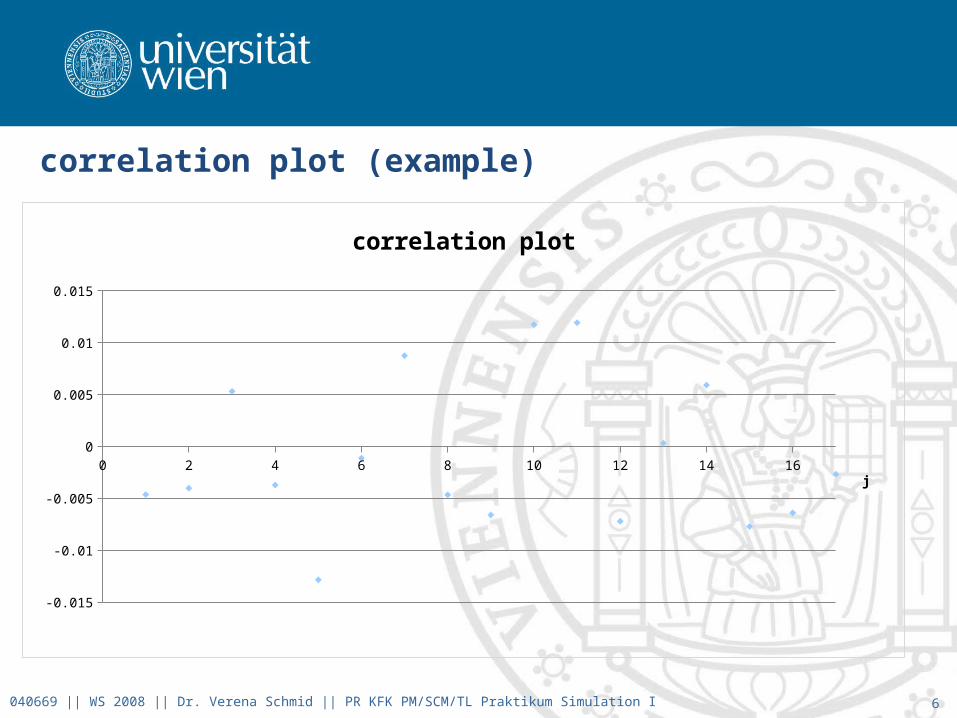
correlation plot
• graph of sample correlation
– estimate of the true correlation between two observations that are j
observations apart in time
– if observations X1, X2, … , Xn are independent
then ½j = 0 for j = 1, 2, …, n-1
- estimates won’t be exactly zero, even if Xi’s are independent, since its
an observation of a random variable
- if estimates differ from 0 by a significant amount, then its strong
evidence that the Xi’s are not independent040669 || WS 2008 || Dr. Verena Schmid || PR KFK PM/SCM/TL Praktikum Simulation I
6
correlation plot (example)
040669 || WS 2008 || Dr. Verena Schmid || PR KFK PM/SCM/TL Praktikum Simulation I
0 2 4 6 8 10 12 14 16
-0.015
-0.01
-0.005
0
0.005
0.01
0.015
correlation plot
j

7
correlation plot (example)
040669 || WS 2008 || Dr. Verena Schmid || PR KFK PM/SCM/TL Praktikum Simulation I
0 2 4 6 8 10 12 14 16 18 20
-0.4
-0.2
0
0.2
0.4
0.6
0.8
1
correlation plot
j
8
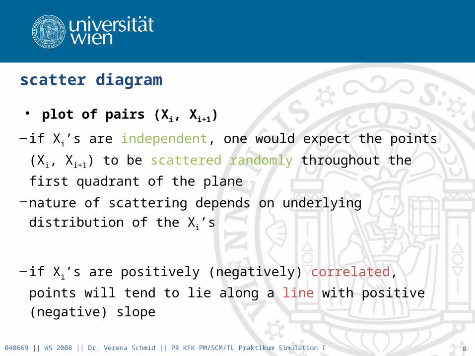
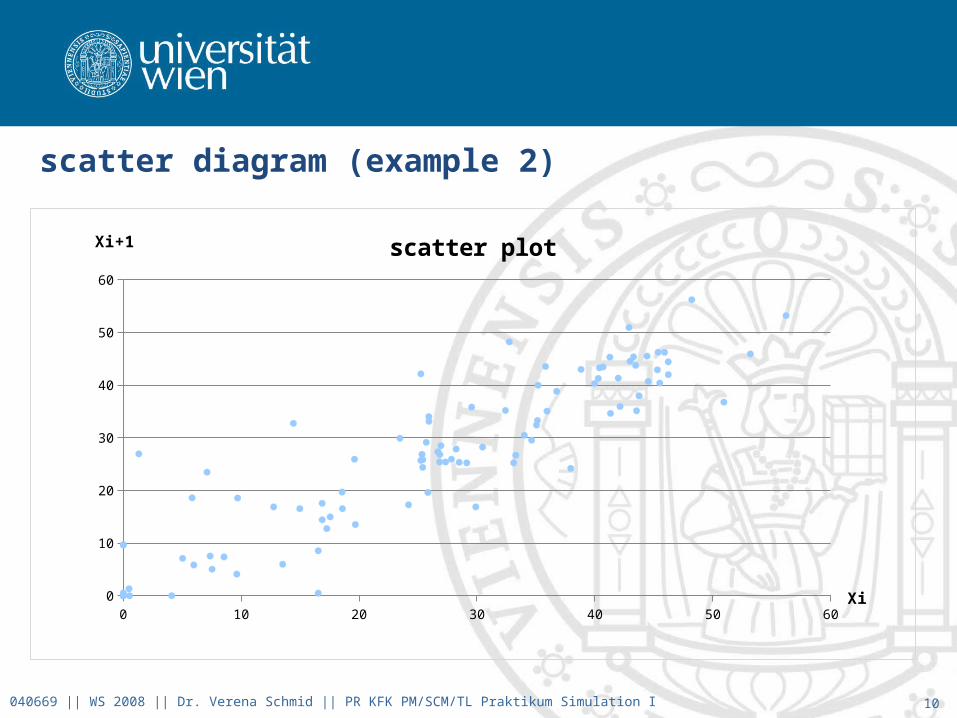
scatter diagram
• plot of pairs (Xi, Xi+1)
– if Xi’s are independent, one would expect the points (Xi, Xi+1) to be
scattered randomly throughout the first quadrant of the plane
–nature of scattering depends on underlying distribution of the Xi’s
– if Xi’s are positively (negatively) correlated, points will tend to lie along a
line with positive (negative) slope
040669 || WS 2008 || Dr. Verena Schmid || PR KFK PM/SCM/TL Praktikum Simulation I

9
scatter diagram (example)
040669 || WS 2008 || Dr. Verena Schmid || PR KFK PM/SCM/TL Praktikum Simulation I
0 0.5 1 1.5 2 2.5 3 3.5 4 4.50
0.5
1
1.5
2
2.5
3
3.5
4
4.5
scatter plot
Xi
Xi+1
10
scatter diagram (example 2)
040669 || WS 2008 || Dr. Verena Schmid || PR KFK PM/SCM/TL Praktikum Simulation I
0 10 20 30 40 50 600
10
20
30
40
50
60
scatter plot
Xi
Xi+1

Specifying Distributionuseful distributions
use values directly
define empirical distribution
fit theoretical distribution
040669 || WS 2008 || Dr. Verena Schmid || PR KFK PM/SCM/TL Praktikum Simulation I 11
12
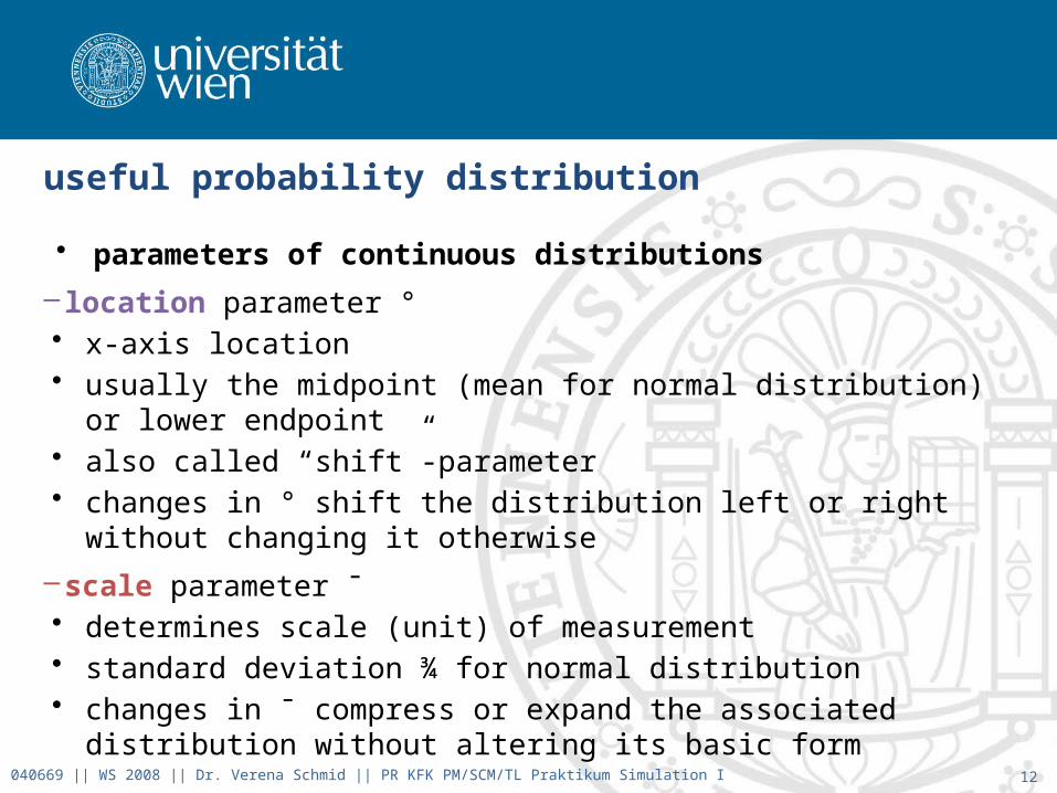
useful probability distribution
• parameters of continuous distributions
– location parameter °• x-axis location• usually the midpoint (mean for normal distribution) or lower endpoint• also called “shift”-parameter• changes in ° shift the distribution left or right without changing it
otherwise
–scale parameter ¯• determines scale (unit) of measurement• standard deviation ¾ for normal distribution• changes in ¯ compress or expand the associated distribution without
altering its basic form
040669 || WS 2008 || Dr. Verena Schmid || PR KFK PM/SCM/TL Praktikum Simulation I

13
useful probability distribution
• parameters of continuous distributions
–shape parameter ®• determines basic form or shape of a distribution within the general
family of distributions of interest• a change in ® generally alters a distribution’s properties (skewness)
more fundamentally than a change in location or scale
040669 || WS 2008 || Dr. Verena Schmid || PR KFK PM/SCM/TL Praktikum Simulation I
14
Approaches to specify distribution
• if data collection on an input random variable is possible
–use data values directly in simulation (trace driven)• only reproduces what happened• seldom enough data to make all simulation runs• useful for model validation
–define empirical distribution• at least (for continuous data) any value between min and max• no values outside the range can be generated • may have irregularities
– fit to theoretical distribution• preferred method• easy to change
040669 || WS 2008 || Dr. Verena Schmid || PR KFK PM/SCM/TL Praktikum Simulation I

Specifying Distributionuseful distributions
use values directly
define empirical distribution
fit theoretical distribution
040669 || WS 2008 || Dr. Verena Schmid || PR KFK PM/SCM/TL Praktikum Simulation I 15
16
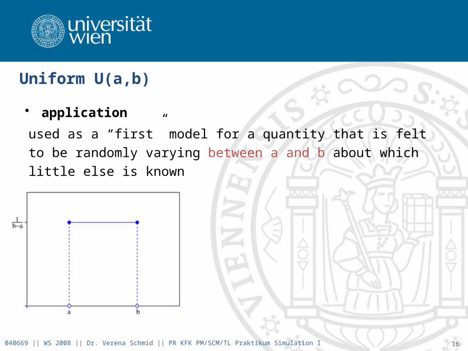
Uniform U(a,b)
• application
used as a “first” model for a quantity that is felt to be randomly varying
between a and b about which little else is known
040669 || WS 2008 || Dr. Verena Schmid || PR KFK PM/SCM/TL Praktikum Simulation I

17
exponential distribution exp(¸)
• application
– interarrival times of entities to a system that occur at a constant rate
– time to failure of a piece of equipment• parameters
– scale parameter ¸ > 0
040669 || WS 2008 || Dr. Verena Schmid || PR KFK PM/SCM/TL Praktikum Simulation I

18
gamma(k, µ)
• application
– time to complete some task (customer service, machine repair)• parameters
– shape parameter k > 0
– scale parameter µ > 0
040669 || WS 2008 || Dr. Verena Schmid || PR KFK PM/SCM/TL Praktikum Simulation I
19
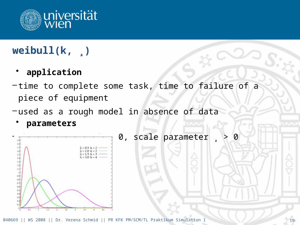
weibull(k, ¸)
• application
– time to complete some task, time to failure of a piece of equipment
–used as a rough model in absence of data• parameters
– shape parameter k > 0, scale parameter ¸ > 0
040669 || WS 2008 || Dr. Verena Schmid || PR KFK PM/SCM/TL Praktikum Simulation I

20
normal N(¹, ¾2)
• application
–errors of various types
–quantities that are the sum of a large number of other quantities• parameters
– location parameter -1 < ¹ < 1 scale parameter ¾ > 0
040669 || WS 2008 || Dr. Verena Schmid || PR KFK PM/SCM/TL Praktikum Simulation I
21
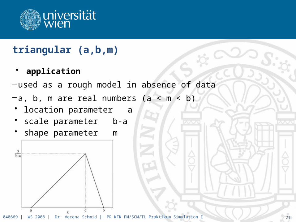
triangular (a,b,m)
• application
–used as a rough model in absence of data
–a, b, m are real numbers (a < m < b)• location parameter a• scale parameterb-a• shape parameter m
040669 || WS 2008 || Dr. Verena Schmid || PR KFK PM/SCM/TL Praktikum Simulation I

22
poisson(¸)
• application
–number of events that occur in an interval of time when events are
occurring at a constant rate
–number of items demanded from inventory
040669 || WS 2008 || Dr. Verena Schmid || PR KFK PM/SCM/TL Praktikum Simulation I

Specifying Distributionuseful distributions
use values directly
define empirical distribution
fit theoretical distribution
040669 || WS 2008 || Dr. Verena Schmid || PR KFK PM/SCM/TL Praktikum Simulation I 23

24
Empirical Distributions
• use observed data themselves to specify distribution directly
–generate random variables from empirical distribution
– (if no theoretical distribution can be fitted)
• define a continuous piecewise-linear distribution function
– sort Xj’s into increasing order
–X(i) denotes the ith smallest value of all Xj’s
040669 || WS 2008 || Dr. Verena Schmid || PR KFK PM/SCM/TL Praktikum Simulation I
25
Empirical Distribution (example)
observation: X1 = 3, X2 = 8, X3 = 18, X4 = 10, X5 = 13, X6 = 6
sorted observation: X(1) = 3, X(2) = 6, X(3) = 8, X(4) = 10, X(5) = 13, X(6) = 18
distribution
F(X(i))
F(X(i)) = (i-1)/(n-1)
F(X(1)) = F(3) = 0/5 = 0
F(X(2)) = F(6) = 1/5
F(X(3)) = F(8) = 2/5
etc…
040669 || WS 2008 || Dr. Verena Schmid || PR KFK PM/SCM/TL Praktikum Simulation I
F(X) if X(i) · X · X(i+1)
F(X) = (i-1)/(n-1) + (X –X(i))/((n-1)*(X(i+1)-X(i))
F(12) = ??interval: X(4) · 12 < X(5)
(n = 6, i = 4)F(12) = 3/5 + 2/(5*3) = 0.68

26
Empirical Distribution (example)
040669 || WS 2008 || Dr. Verena Schmid || PR KFK PM/SCM/TL Praktikum Simulation I
2 4 6 8 10 12 14 16 18 200
0.2
0.4
0.6
0.8
1
x
F(x)

Specifying Distributionuseful distributions
use values directly
define empirical distribution
fit theoretical distribution
040669 || WS 2008 || Dr. Verena Schmid || PR KFK PM/SCM/TL Praktikum Simulation I 27
28
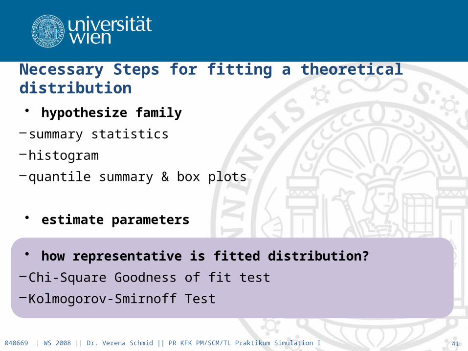
Necessary Steps for fitting a theoretical distribution
• hypothesize family
– summary statistics
–histogram
–quantile summary & box plots
• estimate parameters
• how representative is fitted distribution?
–Chi-Square Goodness of fit test
–Kolmogorov-Smirnoff Test
040669 || WS 2008 || Dr. Verena Schmid || PR KFK PM/SCM/TL Praktikum Simulation I
29
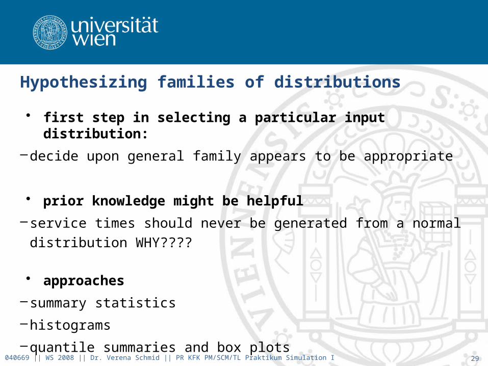
Hypothesizing families of distributions
• first step in selecting a particular input distribution:
–decide upon general family appears to be appropriate
• prior knowledge might be helpful
– service times should never be generated from a normal distribution
WHY????
• approaches
– summary statistics
–histograms
–quantile summaries and box plots
040669 || WS 2008 || Dr. Verena Schmid || PR KFK PM/SCM/TL Praktikum Simulation I
30
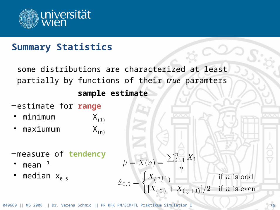
Summary Statistics
some distributions are characterized at least partially by functions of
their true paramters
sample estimate
–estimate for range• minimum X(1)
• maxiumum X(n)
–measure of tendency• mean ¹• median x0.5
040669 || WS 2008 || Dr. Verena Schmid || PR KFK PM/SCM/TL Praktikum Simulation I
31
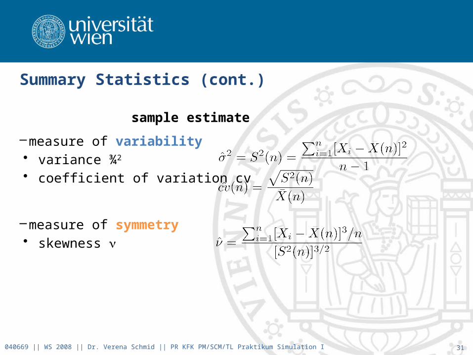
Summary Statistics (cont.)
sample estimate
–measure of variability• variance ¾2
• coefficient of variation cv
–measure of symmetry• skewness n
040669 || WS 2008 || Dr. Verena Schmid || PR KFK PM/SCM/TL Praktikum Simulation I

32
Histograms
• graphic estimate of the plot of the density function corresponding to the distribution of data
–density functions tend to have recognizable shapes in many cases
–graphical estimate of a density should provide a good clue to the
distribution that might be tried as a model for the data
040669 || WS 2008 || Dr. Verena Schmid || PR KFK PM/SCM/TL Praktikum Simulation I
33
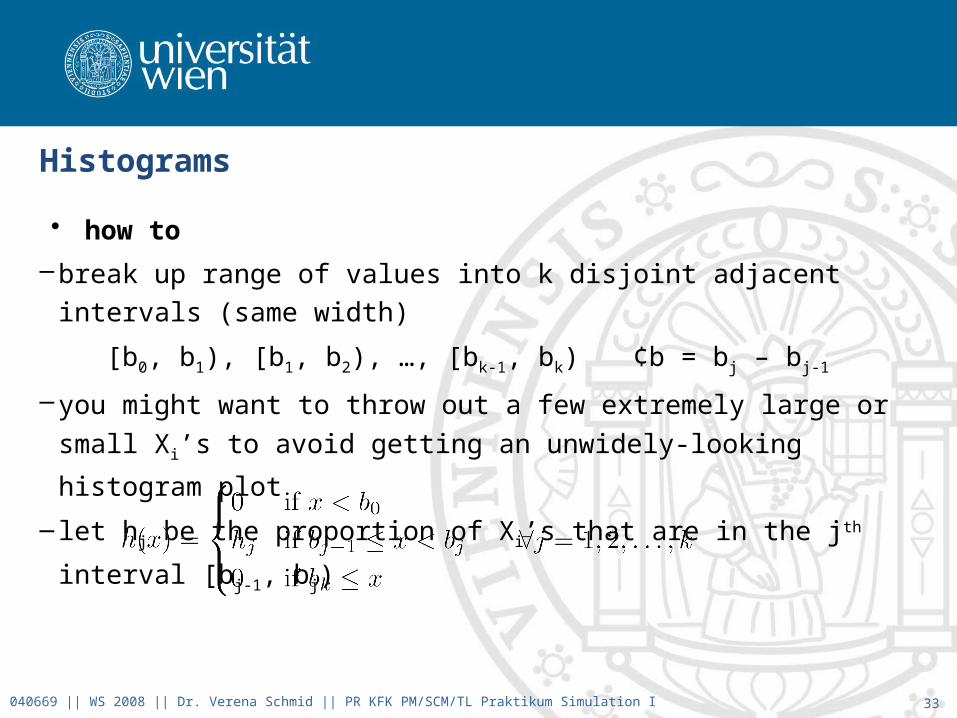
Histograms
• how to
–break up range of values into k disjoint adjacent intervals (same width)
[b0, b1), [b1, b2), …, [bk-1, bk) ¢b = bj – bj-1
– you might want to throw out a few extremely large or small Xi’s to avoid
getting an unwidely-looking histogram plot
– let hj be the proportion of Xi’s that are in the jth interval [bj-1, bj)
–hint: try several values of ¢b and choose the smallest one that gives a
“smooth” histogram040669 || WS 2008 || Dr. Verena Schmid || PR KFK PM/SCM/TL Praktikum Simulation I
34
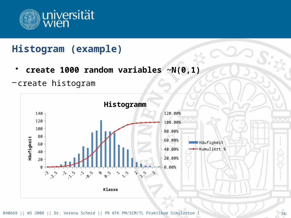
Histogram (example)
• create 1000 random variables ~N(0,1)
– create histogram
040669 || WS 2008 || Dr. Verena Schmid || PR KFK PM/SCM/TL Praktikum Simulation I
-3-2
.5 -2-1
.5 -1-0
.5 00.
5 11.
5 22.
5 30
20
40
60
80
100
120
140
0.00%
20.00%
40.00%
60.00%
80.00%
100.00%
120.00%
Histogramm
Häufigkeit
Kumuliert %
Klasse
Häu
fig
keit

35
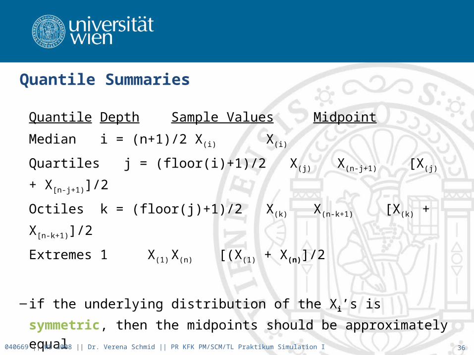
Quantile Summaries
• useful for determining whether the underlying probability density function is skewed to the right or left
– if F(x) is the distribution function for a continuous random variable
–q-quantile of F(x) is that number xq such that F(xq) = q
• median x0.5
• lower/upper quartiles x0.25 / x0.75
• lower/upper octiles x0.125 / x0.875
040669 || WS 2008 || Dr. Verena Schmid || PR KFK PM/SCM/TL Praktikum Simulation I
36
Quantile Summaries
Quantile Depth Sample Values Midpoint
Median i = (n+1)/2 X(i) X(i)
Quartiles j = (floor(i)+1)/2 X(j) X(n-j+1) [X(j) + X[n-j+1)]/2
Octiles k = (floor(j)+1)/2X(k) X(n-k+1) [X(k) + X[n-k+1)]/2
Extremes 1 X(1) X(n) [(X(1) + X(n)]/2
– if the underlying distribution of the Xi’s is symmetric, then the midpoints
should be approximately equal
– if the underlying distribution is skewed to the right (left), then the
midpoints should be increasing (decreasing)040669 || WS 2008 || Dr. Verena Schmid || PR KFK PM/SCM/TL Praktikum Simulation I

37
Box Plots (example)
• graphical representation of quantile summary
– fifty percent of observations fall within the horizontal boundaries of the
box [x0.25, x0.75]
040669 || WS 2008 || Dr. Verena Schmid || PR KFK PM/SCM/TL Praktikum Simulation I
1
0 0.5 1 1.5 2 2.5 3 3.5 4
box plot

38
Necessary Steps for fitting a theoretical distribution
• hypothesize family
– summary statistics
–histogram
–quantile summary & box plots
• estimate parameters
• how representative is fitted distribution?
–Chi-Square Goodness of fit test
–Kolmogorov-Smirnoff Test
040669 || WS 2008 || Dr. Verena Schmid || PR KFK PM/SCM/TL Praktikum Simulation I
39
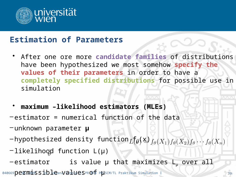
Estimation of Parameters
• After one ore more candidate families of distributions have been hypothesized we most somehow specify the values of their parameters in order to have a completely specified distributions for possible use in simulation
• maximum –likelihood estimators (MLEs)
–estimator = numerical function of the data
–unknown parameter µ
–hypothesized density function fµ(x)
– likelihood function L(µ)
–estimator is value µ that maximizes Lµ over all permissible values of µ
040669 || WS 2008 || Dr. Verena Schmid || PR KFK PM/SCM/TL Praktikum Simulation I

40
Estimation for Parameters (example)
• exponential distribution with unknown parameter ¯ (µ = ¯)
– f¯(x) = (1/¯) e-x/¯ for x ¸ 0
– likelihood function L(¯)
–we seek value of ¯ that maximizes L(¯) over all ¯ > 0
–easier to work with its logarithm
(maximize l(¯) instead of L(¯))
–maximize: set derivative equal to zero and solve for ¯
040669 || WS 2008 || Dr. Verena Schmid || PR KFK PM/SCM/TL Praktikum Simulation I
41
Necessary Steps for fitting a theoretical distribution
• hypothesize family
– summary statistics
–histogram
–quantile summary & box plots
• estimate parameters
• how representative is fitted distribution?
–Chi-Square Goodness of fit test
–Kolmogorov-Smirnoff Test
040669 || WS 2008 || Dr. Verena Schmid || PR KFK PM/SCM/TL Praktikum Simulation I
42
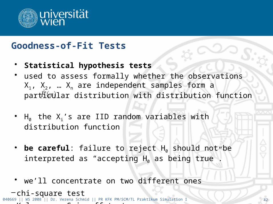
Goodness-of-Fit Tests
• Statistical hypothesis tests• used to assess formally whether the observations X1, X2, … Xn are
independent samples form a particular distribution with distribution function
• H0 the Xi’s are IID random variables with distribution function
• be careful: failure to reject H0 should not be interpreted as “accepting H0 as being true”.
• we’ll concentrate on two different ones
– chi-square test
–Kolmogorov-Smirnoff tests040669 || WS 2008 || Dr. Verena Schmid || PR KFK PM/SCM/TL Praktikum Simulation I

43
Chi-Square Goodness-of-Fit Test
• more formal comparison of a histogram with the fitted density or mass function
• how to
–divide range into k adjacent intervals [a0, a1), [a1, a2), …, [ ak-1, ak)
• how to choose number and size of intervals? ! equiprobable
–determine Nj (number of Xi’s in the jth interval [aj-1, aj)
– compute pj (expected proportion of the Xi’s that would fall in the jth
interval if we were sampling from the fitted distribution
–determine test statistic χ² and reject H0 if its too large
040669 || WS 2008 || Dr. Verena Schmid || PR KFK PM/SCM/TL Praktikum Simulation I
44
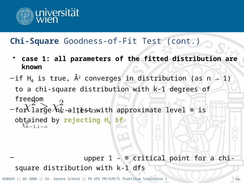
Chi-Square Goodness-of-Fit Test (cont.)
• case 1: all parameters of the fitted distribution are known
– if H0 is true, Â2 converges in distribution (as n → 1) to a chi-square
distribution with k-1 degrees of freedom
– for large n, a test with approximate level ® is obtained by rejecting H0 if
– upper 1 - ® critical point for a chi-square distribution with k-1 dfs
040669 || WS 2008 || Dr. Verena Schmid || PR KFK PM/SCM/TL Praktikum Simulation I

45
Chi-Square Goodness-of-Fit Test (cont.)
•case 2: m parameters had to be estimated to specify fitted distribution
– if H0 is true, then as n ! 1 the distribution function of 2 converges to a
distribution function that lies between the distribution function with k-
1 and k-m-1 degrees of freedom
– the upper 1 - ® critical point of the asymptotic distribution of 2
(in general not known)
– reject H0 if
–do not reject H0 if
–ambiguous situation if• recommendation reject H0 if (conservative)040669 || WS 2008 || Dr. Verena Schmid || PR KFK PM/SCM/TL Praktikum Simulation I
46
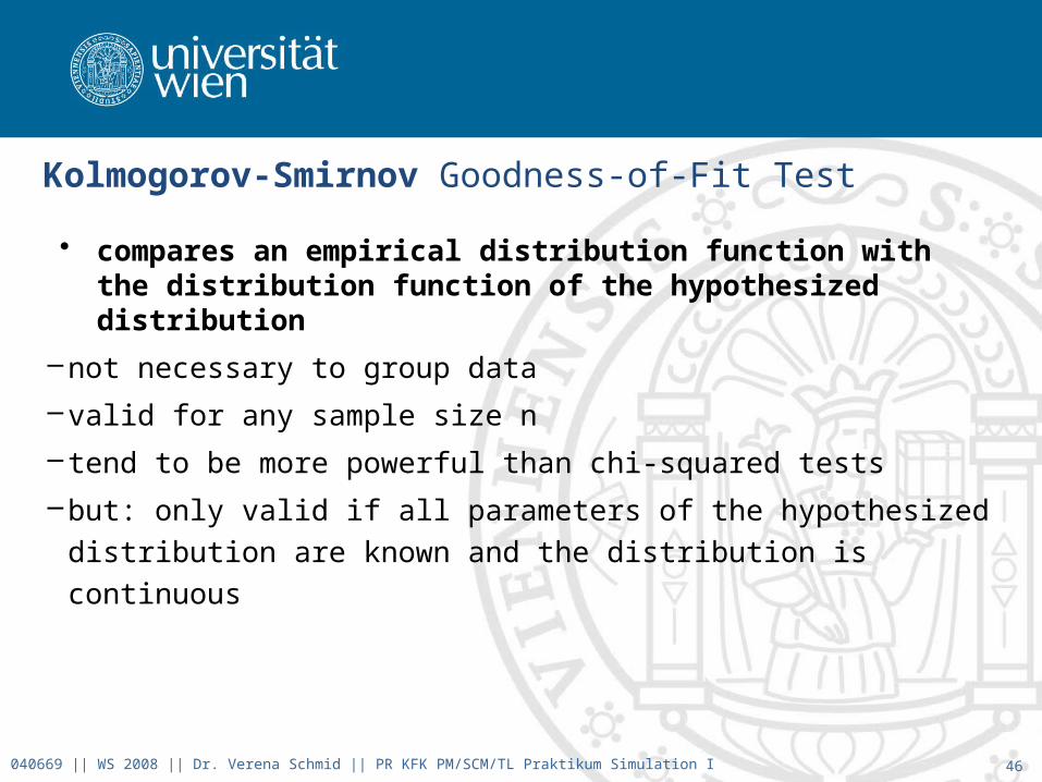
Kolmogorov-Smirnov Goodness-of-Fit Test
• compares an empirical distribution function with the distribution function of the hypothesized distribution
–not necessary to group data
– valid for any sample size n
– tend to be more powerful than chi-squared tests
–but: only valid if all parameters of the hypothesized distribution are
known and the distribution is continuous
040669 || WS 2008 || Dr. Verena Schmid || PR KFK PM/SCM/TL Praktikum Simulation I

47
Kolmogorov-Smirnov Goodness-of-Fit Test (cont.)
• compute tests statistics
–define empirical distribution function
– test statistic Dn corresponds to largest (vertical) distance between
Fn(x) and hypothesized distribution function of
040669 || WS 2008 || Dr. Verena Schmid || PR KFK PM/SCM/TL Praktikum Simulation I

48
Kolmogorov-Smirnov Goodness-of-Fit Test (cont.)
• case 1: all parameters of estimated distribution function are known
–distribution of Dn does not depend on (if is continuous)
– reject H0 if
–c1-® (does not depend on n) given in the following table
1 - ® 0.85 0.9 0.95 0.975 0.99
c1-® 1.138 1.224 1.358 1.48 1.628
040669 || WS 2008 || Dr. Verena Schmid || PR KFK PM/SCM/TL Praktikum Simulation I
49
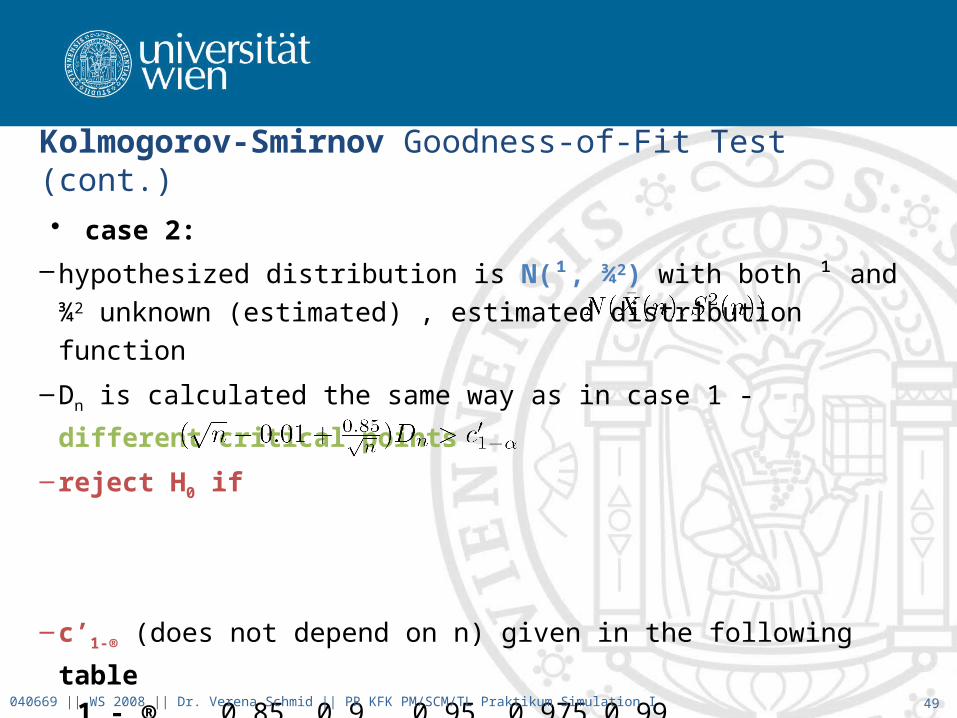
Kolmogorov-Smirnov Goodness-of-Fit Test (cont.)
• case 2:
–hypothesized distribution is N(¹, ¾2) with both ¹ and ¾2 unknown
(estimated) , estimated distribution function
–Dn is calculated the same way as in case 1 - different critical points
– reject H0 if
–c’1-® (does not depend on n) given in the following table
1 - ® 0.85 0.9 0.95 0.975 0.99
c’1-® 0.775 0.819 0.895 0.955 1.035
040669 || WS 2008 || Dr. Verena Schmid || PR KFK PM/SCM/TL Praktikum Simulation I

50
Kolmogorov-Smirnov Goodness-of-Fit Test (cont.)
• case 3
–hypothesized distribution is exponentially distributed (exp(¸))
–with ¸ unknown (estimated using )
–estimated distribution function
– reject H0 if
–c’’1-® (does not depend on n) given in the following table
1 - ® 0.85 0.9 0.95 0.975 0.99
c’1-® 0.926 0.990 1.094 1.19 1.308
040669 || WS 2008 || Dr. Verena Schmid || PR KFK PM/SCM/TL Praktikum Simulation I


