Selecting Instrumentation - download.ni.com

ni.com/automatedtest

CONTENTS

Introduction

Analog and RF Instrumentation

Digital Instrumentation

Form Factor

Next Steps

FuNDAmENTAlS OF BuIlDINg A TEST SySTEm

Selecting Instrumentation

http://ni.com/automatedtest

http://www.ni.com


Selecting Instrumentation2

IntroductionEngineers can generally agree on the high importance of the adage “pick the right tool for the job.” using the wrong tool can waste time and compromise quality, whereas the right tool can deliver the correct result in a fraction of the time.

When building automated test systems, the primary tools at your disposal come in the form of measurement instruments. These instruments include known commodities like digital mulitmeters (Dmms), oscilloscopes, and waveform generators as well as a variety of new and changing categories of products like vector signal transceivers and all-in-one oscilloscopes. To select instrumentation, a skilled test engineer must be knowledgeable and proficient in navigating:

■■ Technical measurement requirements of the device under test (DuT)■■ Key instrument specifications that will influence an application■■ Various categories of instrumentation available and the trade-offs in capabilities, size, price,

and so on■■ Nuanced differences between product models within a given instrument category

Picking the right tool for the job is much easier said than done, specifically when it comes to navigating and evaluating the many trade-offs at play. In this guide, see the major categories of instruments available, and learn about common selection criteria to help you narrow in on the best choice for your application.




Analog and RF InstrumentationThe landscape of analog and RF test instruments is very broad with thousands of models across hundreds of product categories. At the same time, it is also predictably governed by the laws of physics—specifically, the fundamentals of noise and bandwidth manifest in the form of amplifier technology and analog-to-digital converters (ADCs) that are used to create instruments. These fundamental physics limitations create a very discernable trade-off in the precision of a measurement compared to the speed at which it can be acquired. Shown below is a view of how that speed versus resolution trade-off has evolved over time as technology has progressed in both traditional and modular instruments.

Analog and RF Instrument CategoriesThe curve in Figure 1 represents examples from a variety of different instrument categories. Dmms provide high accuracy at low speeds at the top left of the chart, oscilloscopes provide high-frequency acquisitions at lower resolutions on the bottom right of the chart, and DAQ products offer higher channel densities and lower cost in the bottom left.

To narrow in on which category of instrument to begin looking into, first consider a couple of key questions about your measurement task:

■■ What is the direction of the signal? (input, output, or both)■■ What is the frequency of the signal? (DC, kilohertz, megahertz, or gigahertz)

given the answers to those two key questions on directionality and speed, there’s generally a natural starting point for the instrument category you should consider, which Table 1 can best describe.

Figure 1. Resolution Versus Sample Rate for Instrumentation

28

26

24

22

20

18

16

14

12

10

8

6

41 10 100 1K 10K 100K 1m 10m 100m 1g 10g 100g

SAmPlE RATES (SAmPlES/S)

RE

SO

luTI

ON

(BIT

S)

TRADITIONAl INSTRumENTS NI PRODuCTS

2016 1995

2016 RF 2016

2016RF




This chart, although helpful, is far from an exhaustive list of instrument types, especially regarding vertical or specific-purpose instruments. Some noteworthy areas that the table does not cover include:

■■ Specialty DC instruments such as electrometers, microohmmeters, nanovoltmeters, and so on■■ Audio band analysis and generation (also known as dynamic signal analyzers) ■■ Specialty analog products including pulse generators, pulser/receivers, and more

Key Specifications to ConsiderAfter you have narrowed a measurement task to a specific instrument category, the next step is to weigh the trade-offs among products within that category regarding requirements including:

■■ Signal ranges, isolation, and impedance—First, make sure an instrument’s input signal range is large enough to capture the signals of interest. Additionally, consider an instrument’s input impedance, which affects the loading and frequency performance of the measurement setup, and an instrument’s isolation from ground, which impacts noise immunity and safety.

■■ Analog bandwidth and sample rate—Next, make sure that the instrument can pass through the signals of interest based on their analog bandwidth (represented in kilohertz, megahertz, or gigahertz) and that the ADC can sample fast enough to capture the signal of interest (represented in samples per second such as kilosamples per second, million samples per second, or gigasamples per second).

■■ Measurement resolution and accuracy—Finally, evaluate multiple aspects in an instrument’s vertical specifications that influence the quality of the measurement such as ADC resolution (digital quantization of analog signals, generally between 8-bit up to 24-bit), measurement accuracy (maximum measurement error over time and temperature, generally expressed in percent or parts per million), and measurement sensitivity (the smallest detectable change, generally expressed in absolute units such as microvolts)

Table 1. Analog Instrumentation Categories

DC AND POWERlOW-SPEED

ANAlOgHIgH-SPEED

ANAlOgRF AND WIRElESS

INPuT, mEASuRE Digital multimeter Analog Input, Data Acquisition (DAQ)

Oscilloscope, Frequency Counter

RF Analyzer Power meter

(Spectrum Analyzer, Vector Signal Analyzer)

OuTPuT, gENERATEProgrammable Power Supply

Analog OutputFunction/Arbitrary

Waveform generator (FgEN, AWg)

RF Signal generator (Vector Signal

generator, CW Source)

INPuT AND OuTPuT ON THE SAmE

DEVICEDC Power Analyzer

multifunction Data Acquisition

(multifunction DAQ)

All-in-One Oscilloscope

Vector Signal Transceiver (VST)

INPuT AND OuTPuT ON THE SAmE PIN

Source measure unit (Smu)

lCR meter Impedance AnalyzerVector Network Analyzer (VNA)




Instruments that don’t comprise in these functional dimensions of range, accuracy, and speed will likely present other trade-offs in terms of price, size, power consumption, and channel density—all of which influence an instrument’s utility.

Figure 2 shows a simplified view of the analog input path of a generic measurement instrument with four key input stages, the instrument specs those stages influence, and the example instrument specifications of a typical Dmm and a typical oscilloscope as influenced by that stage.

The above simplification can be a helpful construct to sift through instrument specifications, which are often presented using a variety of different nomenclatures across instrument categories and across instrument vendors. These stages are often interdependent in influencing key specifications. For instance, the input amplifier can also influence the input bandwidth and the effective resolution of an instrument. Similarly, the input impedance of an instrument can have major effects on the bandwidth.

Figure 2. Analog Instrumentation Input Stages

INPuT ISOlATION AND TERmINATION

INPuT COuPlINg AND FIlTERINg

INPuT AmPlIFIERANAlOg-TO-DIgITAl CONVERTER (ADC)

Specifications Determined

Isolation Input Impedence

AC/DC Coupling Analog Bandwidth

Max Voltage Range Min Voltage Sensitivity

Sample Rate Resolution

Example Dmm:Isolated up to 300 V

Cat II 10 mΩ (Selectable)

DC coupled 200 kHz bandwidth

up to 300 V input down to 10 nV

sensitivity

10k Hz reading rate 6.5-digital (24-bit)

resolution

Example Oscilloscope:

ground referenced 50 Ω or 1 mΩ

(Selectable)

DC or AC coupled (Selectable)

350 mHz bandwidth

up to 40 Vpp input down to 1 mV

sensitivity

up to 5 gS/s sample rate 8-bit resolution

InputTo PC




Analog and RF Instrument CategoriesAs you compare the measurement requirements of your DuT and the capabilities of the instruments you’ll use to test them, keep in mind the following critical ratios.

Test Accuracy Ratio = 4:1When testing a component, such as a voltage reference, make sure that the accuracy of your measurement equipment is substantially larger than the accuracy of the component being measured. If this criterion is not satisfied, measurement error can be significantly caused by both the DuT and the test equipment, making it impossible to know the true source of error. Because of this, the concept of test accuracy ratio (TAR) is employed to illustrate the relative accuracy of the measurement equipment and the component under test.

Acceptable values for TAR are four and above, depending on the test being performed and the test certainty that is required.

TAR = Wanted Accuracy of the Component Under Test

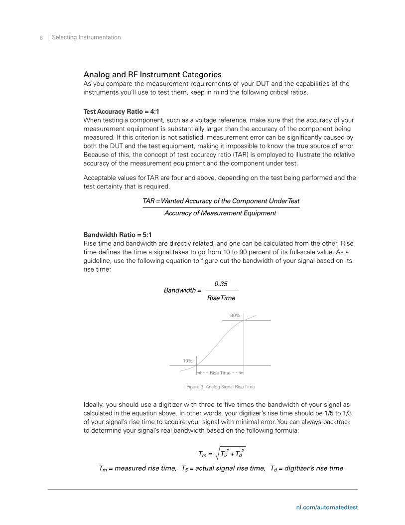
Bandwidth Ratio = 5:1Rise time and bandwidth are directly related, and one can be calculated from the other. Rise time defines the time a signal takes to go from 10 to 90 percent of its full-scale value. As a guideline, use the following equation to figure out the bandwidth of your signal based on its rise time:

0.35

Ideally, you should use a digitizer with three to five times the bandwidth of your signal as calculated in the equation above. In other words, your digitizer’s rise time should be 1/5 to 1/3 of your signal’s rise time to acquire your signal with minimal error. you can always backtrack to determine your signal’s real bandwidth based on the following formula:

Tm = T52 + Td

2

Tm = measured rise time, T5 = actual signal rise time, Td = digitizer’s rise time

Figure 3. Analog Signal Rise Time

Rise Time

90%

10%

Accuracy of Measurement Equipment

Rise TimeBandwidth =




Time Domain Sampling Ratio = 10:1Whereas bandwidth describes the highest frequency sine wave that can be digitized with minimal attenuation, sample rate is simply the rate at which the ADC in the digitizer or oscilloscope is clocked to digitize the incoming signal. Sample rate and bandwidth are not directly related; however, there is a general rule for the wanted relationship between these two important specifications:

Digitizer’s real-time sample rate = 10 times input signal bandwidth

Nyquist theorem states that to avoid aliasing, the sample rate of a digitizer needs to be at least twice as fast as the highest frequency component in the signal being measured. However, sampling at just twice the highest frequency component is not enough to accurately reproduce time-domain signals. To accurately digitize the incoming signal, the digitizer’s real-time sample rate should be at least three to four times the digitizer’s bandwidth. To understand why, look at the figure below and think about which digitized signal you would rather see on your oscilloscope.

Although the actual signal passed through the front-end analog circuitry is the same in both cases, the image on the left is undersampled, which distorts the digitized signal. On the contrary, the image on the right has enough sample points to accurately reconstruct the signal, which results in a more accurate measurement. Because a clean representation of the signal is important for time domain applications such as rise time, overshoot, or other pulse measurements, a digitizer with a higher sample benefits these applications.

Digital InstrumentationIn the context of electronic functional test, digital instrumentation serves the purpose of interfacing with digital protocols and testing the electrical characteristics and communication link characteristics of those protocols. One of most critical aspects influencing the available instrumentation for a given task is parallel versus serial digital communications.

Figure 4. The image on the right shows a digitizer with a sufficiently high sample rate to accurately reconstruct the signal, which will result in more accurate measurements.

Rise Time

90%

10%

Rise Time

90%

10%




Parallel Versus Serial StandardsSerial standards have been gaining in popularity because of the physical limitation on the clock rates of parallel buses at around 1 gHz to 2 gHz. This is because of skew introduced by individual clock and data lines that cause bit errors at faster rates. High-speed serial buses send encoded data that contains both data and clocking information in a single differential signal, allowing you to avoid speed limitations in parallel buses. Serializing the data and sending at faster speeds allows pin counts of integrated circuits (ICs) to be reduced, which helps decrease size. Furthermore, because the serial lanes can operate at a much faster clock speed, they can also achieve better data throughput than what was possible with parallel buses.

1 PCI 64-bit/33 mHz

2 PCI 64-bit/66 mHz

3 PCI 64-bit/100 mHz

4 Front Panel Data Port

5 EISA

6 PCI 32-bit/33 mHz

7 PCI 32-bit/66 mHz

8 IDE (ATA PIO 0)

9 ATA PIO 1

10 ATA PIO 2

11 ATA PIO 3

12 ATA PIO 3 ISA 16-bit/8.33 mHz

13 ultra-2 wide SCSI

14 RapidIO gen1.1

15 gPIB

16 SCSI ISA 8-bit/4.77 mHz

1 PCIe gen1x16

2 PCIe gen2x16

3 Serial RapidIO gen2

4 PCIe gen3x16

5 PCIe gen1x8

6 PCIe gen2x8

7 PCIe gen3x8

8 JESD204B

9 PCIe gen1x4

10 Serial RapidIO gen1.3

11 PCIe gen2x4

12 DisplayPort

13 PCIe gen3x4

14 HDmI 1.0 DVI

15 HDmI 1.3

16 HDmI 2.0

17 SD-SDI

18 gigabit Ethernet

19 SATA 1.0

20 Serial FPDP PCIe gen1x1

21 SATA 2.0 3g-SDI JESD204A 10 gigabit Ethernet

22 PCIe gen2x1 uSB 3.0

23 SATA 3.0

24 PCIe gen3x1

25 uSB 3.1

1

4

8 9 10 11 12 13

14 15 16

5 6 7

2 364

32

16

8

4

2

11 m 10 m 100 m 1,000 m 10,000 m 10,0000 m

ClOCK FREQ (Hz) or lINE RATE (bps)

Nu

mB

ER

OF

lAN

ES 1

5

9 10 1112 13

6 7

1415 16 17

18 19 20 212223 24 25 26 27

8

2 3 4

Parallel

Serial

BuS STANDARDS

Parallel Bus Serial Bus

Figure 5. This chart shows well-known bus standards and their respective numbers of lanes versus line rates. The serial standards are capable of much higher line rates than the parallel standards, leading to higher throughput.




Digital Instrument CategoriesAs with analog instrumentation, you can quickly narrow your options for digital instrumentation using a couple of key questions:

■■ What task do you need to accomplish? (digital interfacing, custom digital interfacing, or electrical and timing test)

■■ How fast is the link? (static and kilobit per second range, megabit per second, or gigabit per second)

Hardware Versus Software Timingyou can implement digital communication schemes using two main methods: software timing and hardware timing. Software-timed applications do not use any type of clock for input or output. The software controls the I/O, and a programming language controls the timing through software. This programming language typically runs on an OS, which could take up to milliseconds to execute software calls. For software timing, you use the OS timer to determine the rate of timed actions. generally, low-speed applications, such as monitoring and controlling alarms, motors, and enunciators, use software timing.

you can choose from two types of software-timed communication: deterministic control and nondeterministic control. using a real-time OS, you can achieve precision of up to 1 µs; however, real-time OSs do not make communications faster, only more deterministic. Non-real-time systems, such as microsoft Windows, are nondeterministic. In these systems, the time taken for software commands to execute in hardware is inconsistent and could take multiple milliseconds. Factors such as computer memory, processor speed, and other applications running on the OS could affect the execution time.

Table 2. Digital Instrumentation Categories

STATIC, lOW SPEEDSyNCHRONOuS AND

HIgH-SPEED PARAllEl (100 mBITS/S RANgE)

HIgH-SPEED SERIAl(10 gBITS/S RANgE)

INTERFACE(STANDARD)

low-Speed Standard Interface Card (I2C, C) Synchronous Protocol Interface

(ARINC 429, CAN, gPIB, I2C, SPI)

Interface Card (10 gigabit Ethernet, Fibre Channel, PCI Express, and

so on)

INTERFACE (CuSTOm) Digital I/O (gPIO)Digital Waveform generator/ Analyzer, Pattern generator

FPgA-Based High-Speed Serial Interface

Aurora, Serial Rapid I/O, JESD204b

ElECTRICAl TEST AND TImINg TEST

(BASIC INTERFACE)

Pin Electronics Digital, Per-Pin Parametric measurement unit (PPmu)

BERT, Oscilloscope




Hardware-timed devices, in contrast, use the rising or falling edges of a clock for deterministic generation or acquisition. you can use this kind of timing to acquire or generate digital data at rates in the gigabit per second range with very high determinism, and you can reliably output data at predetermined locations.

Applications that use hardware timing include the following:

■■ Chip testing■■ Protocol emulation and testing■■ Digital video and audio testing■■ Digital electronics testing

Clock RateAn important consideration for hardware-timed digital applications is clock speed. The maximum speed that a device can achieve is difficult to compensate for if it is inadequate. you can achieve up to 200 mHz sampling rates for single-ended signals and up to 200 mHz for differential signals using NI high-speed digital I/O devices, thus enabling tests including protocol, digital audio and video, and digital electronic. For scenarios where a device might not meet the necessary clock rate requirements on a serial data stream, you can use serializers/deserializers (SERDES) to acquire higher frequency digital signals. However, depending on the type of SERDES you use, incorporating a SERDES might reduce the number of available lines.

Figure 6. With hardware-timed operations, you can take advantage of real-time, deterministic digital signal output.

Data

Clock




Form FactorIn addition to understanding the analog front end required to physically make the correct measurement, you need your instruments to be stable, repeatable, fast, and PC-connected—that’s part of the job. This brings you to a decision regarding the setting/environment:

■■ For the bench and lab—Accuracy, repeatability, low-level control, ease of setup, and ability to automate for repetitive tests

■■ For the manufacturing floor—Speed, throughput, accuracy, optimization through programming interface, and debugging

Clearly, there are similarities and differences in how you’d select instrumentation across the lab versus the manufacturing floor. you typically evaluate instrument form factors across a set of key success criteria for the end deployment. Below is a typical set of evaluation criteria you might see for a manufacturing environment.

Selecting Bus TypeToday, uSB, PCI Express, and Ethernet/lAN have gained attention as attractive communication options for instrument control. Some test and measurement vendors and industry pundits have claimed that one of these buses, by itself, represents a solution for all instrumentation needs. In reality, it is most likely that multiple bus technologies will continue to coexist in future test and measurement systems because each bus has its own strengths.

Table 3. Hardware Deployment Checklist

FuNCTIONAl NEEDS TEST ENgINEERINg NOTES

Instrumentation, I/O needed?

Processing, compute needed?

Data throughput, storage?

Synchronization?

Future requirements?

Number of systems deployed over number of years?

years of planned sustainment?

Number of global sites replicating?

Environmental stability of deployment scenarios?

How is the initial setup, configuration, and repair managed?

Rack mounted?

Size, weight, and power?

Fixture and connectivity?




BandwidthWhen considering the technical merits of alternative buses, bandwidth and latency are two of the most important bus characteristics. Bandwidth measures the rate at which data is sent across the bus, typically in megabytes per second. A bus with high bandwidth can transmit more data in a given period than a bus with low bandwidth. most users recognize the importance of bandwidth because it affects whether their data can be sent across the bus to or from a shared host processor as fast as it is acquired or generated and how much onboard memory their instruments will need. Bandwidth is important in applications such as complex waveform generation and acquisition as well as RF and communications applications. High-speed data transfer is particularly important for virtual and synthetic instrumentation architectures. The functionality and personality of a virtual or synthetic instrument is defined by software; in most cases, this means data must be moved to a host PC for processing and analysis. Figure 7 charts the bandwidth (and latency) of all the instrumentation buses examined in this guide.

Latencylatency measures the delay in data transmission across the bus. By analogy, if you were to compare an instrumentation bus to a highway, bandwidth would correspond to the number of lanes and the speed of travel, while latency would correspond to the delay introduced at the on and off ramps. A bus with low (meaning good) latency would introduce less delay between the time data was transmitted on one end and processed on the other. latency, while less observable than bandwidth, has a direct impact on applications where a quick succession of short, choppy commands is sent across the bus, such as in handshaking between a Dmm and switch, and in instrument configuration.

Figure 7. Bandwidth Versus latency for Instrumentation Buses

10,000

1,000

100

10

110,000 1,000 100 10 1 0.1

DECREASINg lATENCy (µS)

RE

SO

luTI

ON

(BIT

S)

gOOD BETTER BEST

gigabit Ethernet

uSB 3.0

uSB 2.0

gPIB (HS 488)

gPIB (488.1)

PCI/PXI Express 3.0 (x8)



PCI/PXI

VmE/VXI




GPIBThe IEEE 488 bus—commonly known as gPIB—is a proven bus designed specifically for instrument control applications. gPIB has been a robust, reliable communication bus for 30 years and is still the most popular choice for instrument control because of its low latency and acceptable bandwidth. It currently enjoys the widest industry adoption with a base of more than 10,000 instrument models with gPIB connectivity.

With a maximum bandwidth of about 1.8 mbytes/s, it is best suited for communicating with and controlling stand-alone instruments. The more recent, high-speed revision, HS488, increased bandwidth up to 8 mbytes/s. Transfers are message-based, often in the form of ASCII characters. multiple gPIB instruments can be cabled together to a total distance of 20 m, and bandwidth is shared among all instruments on the bus. Despite relatively lower bandwidth, gPIB latency is significantly lower (better) than that of uSB and especially Ethernet. gPIB instruments do not autodetect nor autoconfigure when connected to the system; though gPIB software is among the best available, and the rugged cable and connector are suitable for the most demanding physical environments. gPIB is ideal for automating existing equipment or for systems requiring highly specialized instruments.

USBuSB has become popular in recent years for connecting computer peripherals. That popularity has spilled over into test and measurement with an increasing number of instrument vendors adding uSB device controller capabilities to their instruments. Though most laptops, desktops, and servers may have several uSB ports, those ports usually all connect to the same host controller, so the uSB bandwidth is shared among all the ports.

latency for uSB falls into the better category (between Ethernet at the slow end and PCI and PCI Express at the fast end), and cable length is limited to 5 m. uSB devices benefit from autodetection, which means that unlike other technologies, such as lAN or gPIB, uSB devices are immediately recognized and configured by the PC when a user connects them. uSB connectors are the least robust and least secure of the buses examined here. External cable ties may be needed to keep them in place.

uSB devices are well suited for applications with portable measurements, laptop or desktop data logging, and in-vehicle data acquisition. The bus has become a popular communication choice for stand-alone instruments because of its ubiquity on PCs and especially its plug-and-play ease of use. The uSB Test and measurement Class (uSBTmC) specification addresses the communication requirements of a broad range of test and measurement devices.




PCIPCI and PCI Express achieve the best bandwidth and latency specifications among all the instrumentation buses examined here. PCI bandwidth is 132 mbytes/s, with that bandwidth shared across all devices on the bus. PCI latency performance is outstanding—benchmarked at 700 ns, compared to 1 ms in Ethernet. PCI uses register-based communication. unlike the other buses mentioned here, PCI does not cable to external instruments. Instead, it is an internal PC bus used for PC plug-in cards and in modular instrumentation systems, such as PXI, so distance measures do not directly apply. Nonetheless, the PCI bus can be extended by up to 200 m by the use of NI fiber-optic mXI interfaces when connecting to a PXI system. Because the PCI connection is internal to the computer, it is probably fair to characterize the connector robustness as being constrained by the stability and ruggedness of the PC in which it resides.

PXI modular instrumentation systems, which are built around PCI signaling, enhance this connectivity with a high-performance backplane connector and multiple screw terminals to keep connections in place. Once booted with PCI or PXI modules in place, Windows automatically detects and installs the drivers for modules. In general, PCI instruments can achieve lower costs because they rely on the power source, processor, display, and memory of the PC that hosts them rather than incorporating that hardware in the instrument itself.

PCI ExpressPCI Express is similar to PCI. It is the latest evolution of the PCI standard. Therefore, much of the above evaluation of PCI applies to PCI Express as well.

The main difference between PCI and PCI Express performance is that PCI Express is a higher bandwidth bus and gives dedicated bandwidth to each device. Of all the buses covered in this guide, only PCI Express offers dedicated bandwidth to each peripheral on the bus. gPIB, uSB, and lAN divide bandwidth across the connected peripherals. Data is transmitted across point-to-point connections called lanes at 250 mbytes/s per direction for gen 1 link. Each PCI Express link can be composed of multiple lanes, so the bandwidth of the PCI Express bus depends on how it is implemented in the slot and device. A x1 (by 1) link provides 250 mbytes/s, a x4 link provides 1 gbyte/s, and a x16 link provides 4 gbytes/s dedicated bandwidth. PCI Express achieves software backward compatibility, meaning that users moving to the PCI Express standard can preserve their software investments in PCI. PCI Express is also extensible by external cabling.

High-speed, internal PC buses were designed for rapid communication. Consequently, PCI Express is an ideal bus choice for high-performance, data-intensive systems where large bandwidth is required and for integrating and synchronizing several types of instruments.




Ethernet/LAN/LXIEthernet has long been an instrument control option. It is a mature bus technology and has been widely used in many application areas outside test and measurement. 100BASE-T Ethernet has a theoretical max bandwidth of 12.5 mbytes/s. gigabit Ethernet, or 1000BASE-T, increases the max bandwidth to 125 mbytes/s. In all cases, Ethernet bandwidth is shared across the network. At 125 mbytes/s gigabit Ethernet is theoretically faster than Hi-Speed uSB, but this performance quickly declines when multiple instruments and other devices are sharing network bandwidth. Communication along the bus is message-based with communication packets adding significant overhead to data transmission. For this reason, Ethernet has the worst latency of the bus technologies featured in this guide.

Nonetheless, Ethernet remains a powerful option for creating a network of distributed systems. It can operate at distances up to 85 m to 100 m without repeaters and has no distance limits with repeaters. No other bus has this range of separation from the controlling PC or platform. As with gPIB, autoconfiguration is unavailable on Ethernet/lAN. you must manually assign an IP address and subnet configuration to your instrument. like uSB and PCI, Ethernet/lAN connections are ubiquitous in modern PCs. This makes Ethernet ideal for distributed systems and remote monitoring. It is often used in conjunction with other bus and platform technologies to connect measurement system nodes. These local nodes may themselves be composed of measurement systems relying on gPIB, uSB, and PCI. Physical Ethernet connections are more robust than uSB connections, but less so than gPIB or PXI.

lAN eXtenstions for Instrumentation (lXI) is an emerging lAN-based standard. The lXI standard defines a specification for stand-alone instruments with Ethernet connectivity that adds triggering and synchronization features.

Despite the conceptual convenience of designating a single bus or communication standard as the ultimate or ideal technology, history shows that several alternative standards are likely to continue to coexist, because each bus technology has unique strengths and weaknesses. Table 4 compiles the performance criteria from the previous section. It should be clear that no single bus is superior across all measures of performance.

BANDWIDTH (mByTES/S) lATENCy (µS)

RANgE (m) (WITHOuT

EXTENDERS)

SETuP AND INSTAllATION

CONNECTOR RuggEDNESS

gPIB1.8 (488.1) 8 (HS488)

30 20 good Best

uSB 60 (uSB 2.0) Analog Output 5 Best good

PCI (PXI) 132 0.7 Internal PC Bus BetterBetter

Best (for PXI)

PCI EXPRESS (PXI EXPRESS)

250 (x1) 4,000 (x16)

0.7 (x1) 0.7 (x4)

Internal PC Bus BetterBetter

Best (for PXI)

ETHERNET/ lAN/lXI

12.5 (Fast) 125 (gigabit)

1,000 (Fast) 1,000 (gigabit)

100 m good good

Table 4. Bus Performance Comparison




you can exploit the strengths of several buses and platforms by creating hybrid test and measurement systems that combine components from modular instrumentation platforms, such as PXI and stand-alone instruments, that connect across gPIB, uSB, and Ethernet/lAN. One key to creating and maintaining a hybrid system is implementing a system architecture that transparently recognizes multiple bus technologies and takes advantage of an open, multivendor computing platform, such as PXI, to achieve I/O connectivity.

The other key to successfully developing a hybrid system is ensuring that the software you choose at the driver, application, and test system management levels is modular. Though some vendors may offer vertical software solutions for specific instruments, the most useful system architecture is one that breaks up the software functions into interchangeable modular layers so that your system is neither tied to a particular piece of hardware or to a particular vendor. This layered approach provides the best code reuse, modularity, and longevity. For example, Virtual Instrument Software Architecture (VISA) is a vendor-neutral software standard for configuring, programming, and troubleshooting instrumentation systems comprising gPIB, serial (RS232/485), Ethernet, uSB, and/or IEEE 1394 interfaces. It is a useful tool because the API for programming VISA functions is similar for a variety of communication interfaces.

With hybrid systems, you can combine the strengths of many types of instruments, including legacy equipment and specialized devices. Despite the appeal of finding a one-size-fits-all solution for instrumentation, reality requires that you fit the instruments and associated bus technologies to your specific application needs.




Timing and Synchronizationyou can find a good example of integrated timing and synchronization between instruments in the PXI platform, a modular standard for test and measurement. PXI Express maintains the 10 mHz backplane clock as well as the single-ended PXI trigger bus and length-matched PXI star trigger signal that the original PXI specification provides. PXI Express also adds a 100 mHz differential clock and differential star triggers to the backplane to offer increased noise immunity and industry-leading synchronization accuracy (250 ps and 500 ps of module-to-module skew, respectively). NI timing and synchronization modules are designed to take advantage of the advanced timing and triggering technology featured in its PXI and PXI Express chassis.

Next Stepslearn more about the basics of using test and measurement instrumentation by reading the white paper series, Instrument Fundamentals. This series covers topics ranging from analog sampling theory to grounding considerations for improved measurements.

2016 National Instruments. All rights reserved. National Instruments, NI, and ni.com are trademarks of National Instruments. Other product and company names listed are trademarks or trade names of their respective companies.

Figure 8. Example of PXI Chassis Timing and Synchronization Features

NI PXI Express System

Controller

NI PXI Express System Timing

Controller

NI PXI Express Peripheral

NI Hybrid Peripheral

NI PXI-1 Peripheral

10 mHz Clock

SyNC 100

100 mHz Differential

Clock

Star Triggers

Differential Star Triggers

PXI TRIggER BuS (8TTl TRIggERS)

NI PXI-1 NI PXI EXPRESS


http://www.ni.com/white-paper/3214/en/

Date post:	16-Jan-2022
Category:	Documents
Upload:	others
View:	7 times
Download:	0 times

Selecting Instrumentation - download.ni.com

Documents