SAMPLING R. Salminen 1 , M.J. Batista 2 , A. Demetriades 3 , J. Lis 4 , and T. Tarvainen 1 , 1 Geological Survey of Finland, Espoo, Finland 2 Geological and Mining Institute of Portugal, Lisbon, Portugal 3 Institute of Geology and Mineral Exploration, Athens, Greece 4 Polish Geological Institute, Warszawa, Poland Sampling Strategy GTN grid cells The FOREGS sampling grid was based on GTN grid cells developed for the purpose of Global Geochemical Baseline mapping (Darnley et al. 1995). This grid divides the entire land surface of the Earth into 160 km x 160 km cells. The cells have their origin on the equator at the 0 o (Greenwich) meridian. European cells (Figure 1) have identifiers such as N36W01, which is defined as the 36th cell north of the equator and the first cell west of the meridian of Greenwich, each cell having a size of 160 km in north-south direction and on average 160 km in east-west direction Selecting sample sites The sampling procedures including the planning phase is described in detail in the field manual (Salminen, Tarvainen et al. 1998). A list of the GTN cells, which should be sampled was produced beforehand by the Geological Survey of Finland (GTK). On the list the country responsible for the coordination was indicated, too. If the Figure 1. Global Terrestrial Network (GTN) cells in the FOREGS countries. (from Salminen, Tarvainen et al. 1998, Fig. 1, p.11). After this original plan, more cells were introduced to Greece, Italy and Spain to cover the coastal areas.
Transcript
SAMPLING
R. Salminen1, M.J. Batista2, A. Demetriades3, J. Lis4, and T. Tarvainen1,
1Geological Survey of Finland, Espoo, Finland 2Geological and Mining Institute of Portugal, Lisbon, Portugal 3Institute of Geology and Mineral Exploration, Athens, Greece
4Polish Geological Institute, Warszawa, Poland
Sampling Strategy
GTN grid cells The FOREGS sampling grid was based on
GTN grid cells developed for the purpose of Global Geochemical Baseline mapping (Darnley et al. 1995). This grid divides the entire land surface of the Earth into 160 km x 160 km cells. The cells have their origin on the equator at the 0o
(Greenwich) meridian. European cells (Figure 1) have identifiers such as N36W01, which is defined as the 36th cell north of the equator and the first cell west of the meridian of Greenwich, each cell having a size of 160 km in north-south
direction and on average 160 km in east-west direction Selecting sample sites
The sampling procedures including the
planning phase is described in detail in the field manual (Salminen, Tarvainen et al. 1998). A list of the GTN cells, which should be sampled was produced beforehand by the Geological Survey of Finland (GTK). On the list the country responsible for the coordination was indicated, too. If the
Figure 1. Global Terrestrial Network (GTN) cells in the FOREGScountries. (from Salminen, Tarvainen et al. 1998, Fig. 1, p.11). After thisoriginal plan, more cells were introduced to Greece, Italy and Spain tocover the coastal areas.
GTN cell was located in more than one country, then the sampling of that particular cell was coordinated by the country (organisation) in which the centre of the cell was located, and the sampling was carried out according to mutual agreement of the neighbouring countries. Since some of the GTN cells in coastal areas consist of mostly water, it was agreed that in order to obtain as perfect coverage as possible these cells could be included in the sampling programme, but at least three sites should be sampled in order to fulfil the specifications of the IUGS/IAGC “Global Geochemical Baselines” mapping programme. However, in countries such as Greece and Italy, where islands and long coastal areas prevail, it was subsequently agreed to include even GTN cells, where only one or two sites could be sampled, in order to obtain a better coverage for the purposes of the European geochemical baselines atlas.
The GTK provided each country maps of GTN cells with five randomly generated numbered points (Figure 2), according to the following scheme. Point number 1 is located in the NE quadrant of the GTN grid cell, number 2 in the NW quadrant, number 3 in the SW quadrant, number 4 in the SE quadrant, and point number 5 is randomly located in anyone of the four quadrants of the 160 x 160 km grid cell.
Selection of small drainage basins in each GTN cell: The given randomly generated points were used to select the five nearest small drainage basins of <100 km2 in area. From the selected small drainage basins the site for stream water (W) (filtered and unfiltered) and stream sediment (S) sampling was chosen close to the confluence point with the main stream. The residual soil (top and subsoil, T and C), and humus (H) samples were collected from an appropriate site, within the area of the small drainage basin, representing the dominant residual soil type (Figure 3). In case the randomly generated point was situated in the sea or in an unreachable area, the nearest amenable small drainage basin was used. Selection of large drainage basins in each GTN cell: From the larger drainage basin (area 1000-6000 km2), to which the small drainage basin is connected (see Figures 3, 4, and 5), the floodplain
sediment samples, the uppermost 25 cm (F), and the optional lowermost (L) were collected, either from a suitable point near its outlet with the sea or the confluence point with another major river system. If no suitable large size drainage basin was available, the floodplain sediment samples were taken from a smaller drainage basin of minimum size >500 km2. Duplicate sampling
From each country at least one GTN cell was
randomly selected for duplicate sampling. Countries with nine or more GTN cells collected duplicate samples from 2 or more cells. Duplicate samples of each material were taken from one geologically representative small catchment (1, 2, 3, 4 or 5) of the selected GTN cell, and its corresponding floodplain. The procedure of collecting the duplicate samples was identical with that of the normal samples. For residual soil sampling a duplicate composite sample was collected from 3 to 5 new pits dug not further than 10 metres from the original soil sampling pits, and for floodplain sediment sampling a new pit was dug not further than 10 metres from the original floodplain sediment sampling pit.
Figure 2. Example of five randomly generatedsampling points within one 160 km x 160 km grid cell(from Salminen, Tarvainen et al. 1998, Fig. 2, p.13)
Figure 4. Block diagram showing possible sampling sites of GTN sampling media (fromSalminen, Tarvainen et al. 1998, Fig.4, p.14; modified after Strahler 1969).
Figure 3. Selection of sampling sites (modified after Darnley et al. 1995), a schematicoutline of drainage sampling pattern and soil sample pit for the geochemical referencenetwork. The sample pit applies to all residual soil locations. Deep sample near tothe parent rocks (C): a 25 cm thick section within a depth range of 50-200 cm (fromSalminen, Tarvainen et al. 1998, Fig. 3., p.13).
Figure 5. Block diagram showing overburden (soil), colluvium, old and presentday floodplain sediments (from Salminen, Tarvainen et al. 1998, Fig. 5, p.14;modified after Strahler 1969).
Sample identifiers Sample identifiers were formulated as
indicated in the following example. The sample code of the stream sediment sample is:
N43E09S4, where N43E09 = the 43rd GTN cell north of equator
and the 9th cell east of 0 meridian; S = Sample medium symbol for stream
sediment, which is replaced by “W” for stream water, “T” or “C” for top or bottom residual soil, “H” for humus, “F” or “L” for top or bottom floodplain sediment respectively;
4 = Drainage basin number. The letter D was used as a suffix for the
duplicate sample identifier of each sampling medium: N43E09S4D.
The identifier for filtered blank (or zero) water samples was a “0” suffix: N43E09W40.
Photographs
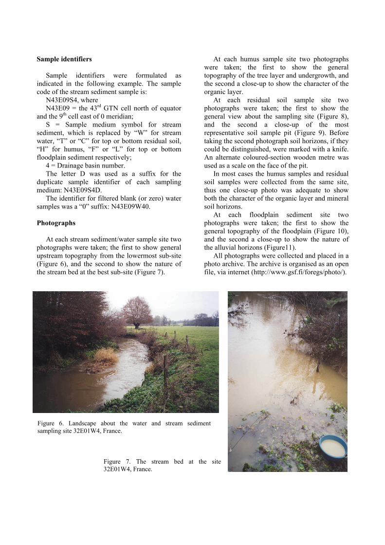
At each stream sediment/water sample site two
photographs were taken; the first to show general upstream topography from the lowermost sub-site (Figure 6), and the second to show the nature of the stream bed at the best sub-site (Figure 7).
At each humus sample site two photographs were taken; the first to show the general topography of the tree layer and undergrowth, and the second a close-up to show the character of the organic layer.
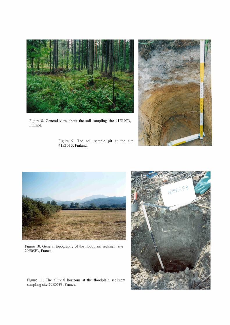
At each residual soil sample site two photographs were taken; the first to show the general view about the sampling site (Figure 8), and the second a close-up of the most representative soil sample pit (Figure 9). Before taking the second photograph soil horizons, if they could be distinguished, were marked with a knife. An alternate coloured-section wooden metre was used as a scale on the face of the pit.
In most cases the humus samples and residual soil samples were collected from the same site, thus one close-up photo was adequate to show both the character of the organic layer and mineral soil horizons.
At each floodplain sediment site two photographs were taken; the first to show the general topography of the floodplain (Figure 10), and the second a close-up to show the nature of the alluvial horizons (Figure11).
All photographs were collected and placed in a photo archive. The archive is organised as an open file, via internet (http://www.gsf.fi/foregs/photo/).
Figure 6. Landscape about the water and stream sedimentsampling site 32E01W4, France.
Figure 7. The stream bed at the site32E01W4, France.
Figure 8. General view about the soil sampling site 41E10T3,Finland.
Figure 9. The soil sample pit at the site41E10T3, Finland.
Figure 11. The alluvial horizons at the floodplain sedimentsampling site 29E05F3, France.
Figure 10. General topography of the floodplain sediment site29E05F3, France.
Sampling
Sampling was carried out in each country by
national teams. Normally one team sampled all sites in each country during one field season between 1997 and 2001. However, in some cases the work was divided in two field seasons as indicated in Table 1. Therefore, it can be stated that the FOREGS geochemical baselines mapping programme represents the end twentieth century state of the surficial environment in Europe.
The number of samples of each type varied
according to the local conditions very much. E.g. humus was not found in the most of
Mediterranean countries. The number of each sample type is summarized country by country in Table 2. Stream water
Running stream water was collected from the small, second order, drainage basins (<100 km2) at the same site as the active stream sediment. In dry terrain, such as Southern Europe, streams have no running water for most of the year. Hence, the sampling, whenever possible, was carried out during the winter and early spring months.
Table 1. Sampling time in each country Albania not reported Austria June 1998 – September 1998 Belgium September 1998 Croatia November 1998
May 1999 – September 1999 Czech Republic September 1998 Denmark September 1999 Estonia June 1999 – September 1999 Finland July 1997 – August 1997
June 1998 – August 1998 France November 1998 – December 1998
March 1999 – October 1999 Germany July 2001 – September 2001 Greece March 2000 – August 2000 Hungary August 1999 – October 1999 Ireland October 1998 Italy April – August 1998
February – March 2001 October 2001
Latvia August 1998 Lithuania September 1997
July 1998 (stream water and stream sediment)
The Netherlands August – September 2000 Norway August – October 1997 Poland May 1999 – September 1999 Portugal October 1998 – March 2000 Slovak Republic July 1998 – November 1998 Slovenia May 2001 Spain June 2000 – November 2000
January 2001 – July 2001 Sweden June, October 1998
October 1999 September – October 2004 (stream sediments)
Switzerland July 1998 – August 1998 UK August-October 1998
Four sub-samples of stream water were separately collected from each site:
• 500 ml bottle unfiltered water for major IC ion analysis,
• 100 ml bottle filtered water for ICP-MS and ICP-AES analysis
• 120 ml bottle unfiltered stream water for mercury analysis, and
• 100 ml bottle filtered water for DOC analysis. The regional laboratories provided the
following equipment to each country: • 500 ml new polyethylene bottles, • 120 ml hardened Nalgene™ trace element free
bottles, • 100 ml new polyethylene bottles,Disposable
Schuell pyrogen free), and • Droplet bottles made of teflon FEP
(fluorinated ethylene propylene). In some cases, instead of the centrally provided
bottles, local bottles were also used, and in a few countries bottles for mercury, ICP and DOC analysis were changed with each other.
Each participant purchased the following equipment:
• pH-meter (recommended device WTW pH90),
• EC-meter (recommended device WTW LF92),
• Hach Model 16900-01 digital titrator with solution delivery straws and appropriate titration cartridges, including 1.6 N and 0.16 N sulphuric acid or 1.6 N and 0.16 N H2SO4 solutions,
• Potassium dichromate solution for Hg preservation: 0.2 g of K2Cr2O7 (Pro analysis, PA, quality) / 100 ml nitric acid HNO3 (Suprapure quality),
• Buffer solutions for calibration of pH-meter, • Concentrated HNO3 65%, density 1.40 kg/l
(recommended Merck Suprapur (R) 100441), • Bromocresol green acid-base indicator
solution (0.1 g of bromocresol green in 14.3 ml of 0.01 M NaOH + 235.7 ml distilled and deionised water),
• Distilled and deionised water and a washing bottle,
• Volumetric flasks, capacity of 100 and 1000 ml,
• Burette or equivalent equipment, 10 ml capacity,
• Plastic 100 ml measuring cylinder (for alkalinity measurements),
• 250 ml plastic conical flask (for alkalinity measurements),
• 2 polyethylene (1 L) decanters for sample water to measure pH and EC,
• Disposable Pasteur-pipettes, • Permanent drawing ink markers, • Cool boxes and their batteries, or a car
refrigerator, and • Rubbish bags.
Table 2. The number of different sample types collected in each country.
Floodplain sediment Humus Sub soil Top soil Stream
Stream water sampling procedure Sampling during rainy periods and flood
events was avoided. The water sample was always taken before the stream sediment sample, for obvious reasons, i.e., during the collection of the stream sediment, fine-grained material is agitated and transported in suspension. The water sample was collected from the first, lowermost stream sediment sampling point (the stream sediment sample is a composite of 5-10 sub-samples taken over a distance of up to 500 m from the lowermost point).
Bottles, decanters, syringes and other equipment were rinsed twice with stream water. Sample identifiers and sample type were marked on the bottle with a permanent ink marker. Field observations were recorded on the field sheet, and sampling position marked on the map.
During sampling disposable plastic gloves were worn all the time on both hands. Further, in order to avoid any kind of metal contamination, no hand jewellery was allowed, and smoking or having the vehicle running during water sampling was strictly prohibited.
To begin with sample identifiers and sample type was marked on the bottle with a permanent ink marker. Bottles, decanters, syringes and other equipment were rinsed twice with unfiltered stream water, and bottles holding filtered water were rinsed twice with filtered stream water. One 500 ml polyethylene bottle and one 120 ml Nalgene™ (high density trace element free polyethylene) bottle, and two 100 ml polyethylene plastic bottles were filled with filtered stream water up to their neck (Figure 12).
pH and EC were measured, and alkalinity estimated by titration at the site.
Alkalinity was measured by titrating 100 ml of water with H2SO4 to pH 4.5. Two methods were used: (A) titration by Hach digital titrator and standard acid cartridges, and (B) titration by ordinary 10 ml burette. In both methods bromocresol green was used as indicator, and normality of sulphuric acid was in both methods either 1.6 N or 0.16 N. Total alkalinity was expressed as mg/l CaCO3. In some cases, sampled stream water was coloured, because of high humus contents, and the titration end-point was thus difficult to observe. In such cases, the pH-meter was used to determine the end-point of titration at a pH of 4.5.
The filled stream water sample bottles were placed in the field in a cool box or a car
refrigerator. One of the 100 ml filtered water samples was
acidified on the same day in the laboratory or in comparable conditions by adding 1.0 ml of conc. HNO3 acid with a droplet bottle. The sample in 120 ml Nalgene™ bottle was acidified and preserved by adding 5 ml of the prepared solution of nitric acid and potassium dichromate solution. Bottles were then stored in a refrigerator and sent to the laboratory soon after sampling.
A blank water sample was collected after every 20th sample (and at least one in every country). Distilled and deionised water was filtered in a 100 ml polyethylene bottle in the same manner as the normal stream water sample. This sample was treated (acidified and handled) like the normal stream water samples. The identifier for a filtered blank zero (0)-sample was: grid cell / W / sample no. / 0, for example, N43E09W40.
Figure 12. Filtration of a stream watersample (photo: Jari Väätäinen, GTK, fromSalminen, Tarvainen et al., 1998, Fig. 6,p.17)
Stream sediment
The active stream sediment sample was
collected from the small, second order, drainage basin (<100 km2) at a suitable site above its confluence point with the main, third order, channel of the large drainage basin, together with the stream water sample.
In order to avoid any kind of metal co
-metal eq
dis
am sediments, wh
mple comprises ma
The regional laboratories provided:
Eac articipant purchased the following
equvy duty elbow length rubber gloves,
en or plastic
• cket,
or containers with lids,
• ing tool - metal free, polyethylene (PE)
• logical hammer for dry areas countries),
• les).
tream sediment sampling procedure The exact site location of the first and last sub-
means of a s
ubber gloves were recommended for pling. All stream
sed
ntamination no hand jewellery or medical dressings were allowed to be worn during sampling. If medical dressings were worn, heavy duty rubber gloves were recommended to be worn at all times to avoid contamination of samples. Metal free polyethylene or unpainted wooden spade/scoop, metal free nylon sieve-mesh housed in an inert wooden or metal free plastic frame and metal free funnels and sample collection containers were used. If contamination sources were observed in the vicinity of the stream, the sampling site was moved to another place.
If it was not possible to use nonuipment (e.g., spades and sieve frames),
unpainted steel equipment was used, but aluminium and brass equipment was not allowed.
Sampling sites were selected at a sufficient tance upstream from confluence points with
higher order streams to avoid sampling sediment that may result from mixing of material from the two channels during flood events.
A system of wet sieving streerever possible, was recommended, but dry
sieving was an alternative method, if wet sieving was not feasible, as is the case of seasonal streams in Mediterranean countries.
Each stream sediment saterial taken from 5-10 points over a stretch of
250-500 m along the stream. Sites were located at least 100 m upstream of roads and settlements. Sampling was started from the stream water sampling point, and the other sub-samples were collected up-stream. A composite sample was made from sub-samples taken from beds of similar nature (ISO 5667-12:1995). Minimum amount of the stream sediment sample was 0.5 kg (dry weight) <0.150 mm material.
• Kraft paper bags, and • Polyethylene bags.
h pipment: • Hea• Metal free polyethylene funnel, • Sieve set with 2 preferably wood
frames containing nylon 2.0 mm mesh and nylon 0.150 mm mesh screens, Metal free gold pan or plastic bu
• Metal free plastic crates, • Metal free plastic buckets
• Metal free plastic or wooden rod, Trenchor polypropylene (PP),
• Permanent drawing ink marker (preferably black or blue),
samples was marked on the field map bymall line perpendicular to the stream flow.
Sampling using wet sieving R
protection throughout samiment sampling equipment (buckets, sieves,
Figure 13. Wet sieving of a stream sediment sample inthe UK (Photo: Fiona Fordyce, BGS from Salminenand Tarvainen et al. 1998, Fig. 7, p.21).
gold pans, funnel, gloves and spade) were thoroughly washed with stream water before and after sampling (Figure 13). In Mediterranean countries, where dry streams were sampled, all equipment was thoroughly washed with spring or tap water after sampling, and dried with clean white cotton waste.
The gold pan or collection bucket was set up in a s
k material int
material required varied sub
ve we
he bottom sieve was wa
ent had be
Sampling using dry sieving tive method used in
Me
other coarse grained ma
mall sea
isaggregated if nec
table position on the stream bank. The sieve with the 0.150 mm aperture nylon cloth was placed in a stable position resting on the gold pan or bucket. The sieve with the 2 mm aperture nylon cloth was set over the 0.150 mm sieve.
In rugged terrain, where collapse bano the channel was probable, sediment from as
near the centre of the stream as possible was collected to avoid sampling bank-slip material. Whereas, in areas of low relief, where active stream sediment in the centre of channels may be enriched in quartz, and depleted in clays was avoided, and other fine-grained material, deposited along stream margins during flood events was regarded as more suitable for sampling.
The amount of coarse stantially, depending on the up stream geology
and terrain. The buckets containing the coarse sediment were mixed thoroughly with a plastic or wooden stirring rod, and carried to the sieving location, where they were left to stand, before draining off excess water. Stream sediment was loaded into the top sieve with the spade or plastic scoop. If more than one bucket of coarse sediment was collected, equal amounts of sediment were loaded into the sieve from each bucket in turn.
The material was rubbed through the top siearing rubber gloves for protection. Large stones
were removed by hand. Once the bottom sieve contained a reasonable quantity of <2 mm sediment, the top sieve was removed and the >2 mm material was discarded.
The <2 mm sediment in tshed and rubbed through the sieve with the aid
of stream water and shaken down. In order to enhance the trace element signature, a minimum amount of water was used to wash the sediment through the bottom sieve, and all washing water was retained in the collection bucket, and the fine-grained sediment was allowed to settle.
Once enough wet fine-grained sedimen collected, the lid was placed securely on the
bucket. The sediment was then allowed to stand until all suspended material had settled, and clear
water sat on top of the sediment. Excess water was carefully decanted. The remaining sediment was thoroughly homogenised and mixed using the plastic stirring rod before being transferred into the Kraft sample bags. At the field base Kraft bags were air dried for as long as possible. Samples were completely dried at <40oC at the Survey base or laboratory. Freeze drying was recommended as this helps to disaggregate the samples.
Dry sieving is an alternaditerranean countries. Since, water was not
available to wet sieve the stream sediment to the required <0.150 mm fraction, a bulk composite sample from 5-10 points was collected. The total dry weight of the composite sample (free of stones and other coarse grained material) should be about 5 kg to ensure that the required amount of 500 grams of <0.150 mm material was obtained after sieving at the domestic lab.
The removal of stones andterial was normally achieved by sieving
through a 5 mm nylon sieve, and collecting the material in a plastic bowl. The use of the 2 mm nylon sieve was not recommended for dry sieving, because it is too small for clay agglomerates and slightly moist samples. However, in completely dry streams, it was possible to sieve enough dry fine-grained material through the 2 mm nylon sieve, and also through the 0.150 mm sieve by careful disaggregation of clay agglomerates.
A special case was the sampling of ssonal streams in Mediterranean countries,
which were sampled with extreme care. Some of the seasonal streams have had no water flow for many years, and the stream bed was covered with fallen bank material in which grass or other plants have grown. Since, active stream sediment must be sampled, the fallen bank material, covering the "old" active stream sediment, was removed by digging down to the old stream bed before taking the sample at each sub-site. The pits were dug near to the centre of the channel.
Stream sediment samples, dessary in a porcelain bowl and sieved through
a 2 mm aperture nylon sieve in the domestic laboratory, were shipped to the Slovak Republic for sieving through a 0.150 mm sieve, homogenisation and sampling of laboratory and archive sub-samples.
of large and small floodplains respectively, according to the catchment basin size distinction made by Darnley et al. (1995). Floodplain and overbank sediments are deposited during flood events in low energy environments (Ottesen et al. 1989, Alexander and Marriott 1999); they should, therefore, be devoid completely of pebbles, which indicate medium energy environments. The surficial floodplain and overbank sediments are normally affected by recent anthropogenic activities, and may be contaminated. Deeper samples, which are optional sample media, normally show the natural background variation. A floodplain sediment, representing the alluvium of the whole drainage basin was collected from the alluvial plain at the lowermost point (near to the mouth) of the large catchment basin (1000-6000 km2).
From eaodplain sediment (sampling depth 0-25 cm)
was collected (Figure 14). Collecting of bottom floodplain sediment from the very bottom layer (the lowermost 25 cm, actual depth noted on the field sheet) of the exposed section, just above the water level of the river was optional. These
samples were not included in the analytical program of the project. Bottom floodplain sediments were collected only in Austria, Belgium, France, Germany, Greece, Norway, Portugal, and Spain.
The amount of sampled sediment was enough to yield a minimum of 0.5 kg of <2 mm grain size sediment.
The regional laboratories provided the following equipment:
• Kraft bags for floodplain sediment, and • Disposable gloves (1 per sample).
Each participant purchased the following equipment:
Sampling tools should have been made of unpainted wood, polyethylene (plastic) or steel (unpainted spade). Containers should have been made of paper or strong polyethylene.
Figure 14. Floodplain sampling in southwestern Finland (Photo: Reijo Salminen, GTK).
Floodplain sediment sampling procedure
pled were noted on the eld observations sheet.
umus and residual soil samples
as not accepted as representing parent ma
44% of the total number of res
The regional laboratories provided the following equipment:
completely filled. A steel or plastic sampling tool
The floodplain sediment sequence was first studied carefully in order to select a suitable section with many layers of fine-grained material, e.g. silty-clay or clayey silt, deposited in a low energy environment. Sites adjacent to roads or ditches (minimum distance 10 m) were avoided. Living surface vegetation, and large roots were removed and a top floodplain sediment sample from 0-25 cm depth was collected preferably from a single floodplain sediment layer. If the layer was thinner than 25 cm, the actual thickness and the number of layers samfi H
Humus and residual or sedentary soil samples were collected at the same site from the small, second order, drainage basin (<100 km2) at a suitable site above its alluvial plain and base of slope, where alluvium and colluvium are respectively deposited. Residual soil developed either directly on bedrock or on till was accepted. Residual soil from areas with agricultural activities was avoided, since the top soil is usually affected by human activities. Colluvium or alluvium w
terial. In the study area, climatic and environmental
conditions for the development of a humus layer were suitable in only the northern European countries. Thus, it was possible to collect humus samples from only
idual soil sites.
• Plastic bags (PE) for humus, • Kraft bags for soil samples, and • Disposable gloves (1 per sample).
Each participant purchased the following equipment:
black or blue), and • Plastic boxes for sample bags.
Sampling tools should be made from unpainted wood, polyethylene (plastic) or steel (unpainted spade). Humus sampling procedure
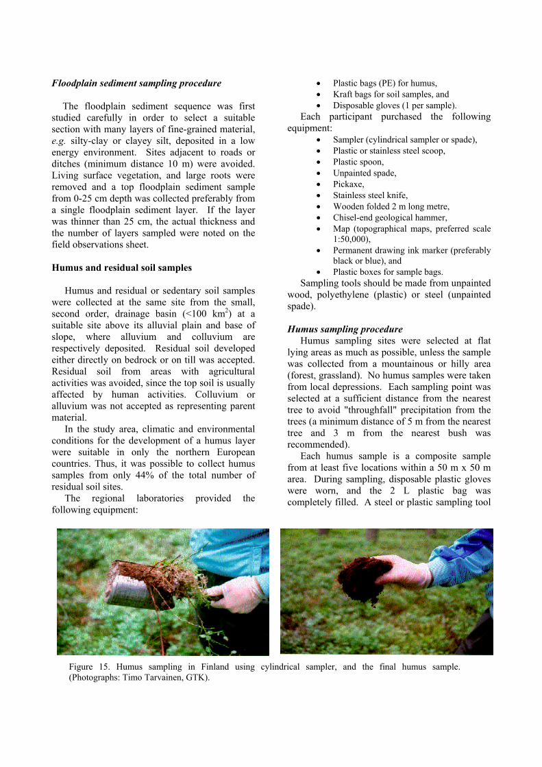
Humus sampling sites were selected at flat lying areas as much as possible, unless the sample was collected from a mountainous or hilly area (forest, grassland). No humus samples were taken from local depressions. Each sampling point was selected at a sufficient distance from the nearest tree to avoid "throughfall" precipitation from the trees (a minimum distance of 5 m from the nearest tree and 3 m from the nearest bush was recommended).
Each humus sample is a composite sample from at least five locations within a 50 m x 50 m area. During sampling, disposable plastic gloves were worn, and the 2 L plastic bag was
Figure 15. Humus sampling in Finland using cylindrical sampler, and the final humus sample.Tarvainen, GTK). (Photographs: Timo
was used for sampling (Figure 15). The living surface vegetation, fresh litter and large roots and rock fragments were carefully removed with plastic gloves. Only the uppermost 3 cm of humus was sampled. The mineral soil layer was carefully removed using a plastic spoon.
Samples were thoroughly air-dried at room temperature, which did not exceed 40oC; the sample was placed on the bag and turned over as necessary using gloves. When samples were properly dried, they were transferred to a new bag, if needed, sealed and sent to the agreed laboratory in The Netherlands.
Residual soil sampling procedure
Each residual soil sample was a composite of 3 to 5 sub samples collected from pits located at a distance of 10-20 metres from each other. Two different depth related samples were taken at each
site: a topsoil sample from 0-25 cm (excluding material from the organic layer where present), and a subsoil sample from a 25 cm thick section within a depth range of 50 to 200 cm (the C soil horizon).
The residual soil sample represents the dominant residual soil type of the selected catchment basin. Minimum distance to roads was 10 m and to ditches 5 m.
Living surface vegetation, fresh litter, large roots and rock fragments (stones) were removed by hand. In case the whole soil profile did not reach the depth of 75 cm, the lower sample was taken from a depth that can be undoubtedly identified as the BC- or C-horizon. The subsoil sample was always collected first, and then the topsoil sample. Thus, avoiding to clean up the surface of the subsoil from fallen top soil material.
References
Alexander, J. & Marriott, S.B., 1999. Introduction. In: S.B. Marriott & J. Alexander (Eds), Floodplains: Interdisciplinary Approaches. The Geological Society, London, Special Publ. No. 163, 1-13.
Darnley, A.G., Björklund, A., Bölviken, B., Gustavsson, N., Koval, P.V., Plant, J.A., Steenfelt, A., Tauchid, M. & Xie Xuejing,, 1995. A Global geochemical database for environmental and resource management. Final report of IGCP Project 259. Earth Sciences 19, UNESCO Publishing, Paris, 122 pp.
Ottesen, R.T., Bogen, J., Bølviken, B. & Volden, T., 1989. Overbank sediment: a representative sample medium for regional geochemical mapping. Journal
of Geochemical Exploration 32, 257-277. Salminen, R., Tarvainen, T., Demetriades, A., Duris,
M., Fordyce, F. M., Gregorauskiene, V., Kahelin, H., Kivisilla, J., Klaver, G., Klein, H., Larson, J. O., Lis, J., Locutura, J., Marsina, K., Mjartanova, H., Mouvet, C., O'Connor, P., Odor, L., Ottonello, G., Paukola, T., Plant, J.A., Reimann, C., Schermann, O., Siewers, U., Steenfelt, A., Van der Sluys, J., Vivo, B. de, & Williams, L., 1998. FOREGS geochemical mapping field manual. Geologian tutkimuskeskus, Espoo. Opas 47, 36 p. + 1 app.
Strahler, A.N., 1969. Physical Geography. 3rd edition. New York – London, John Wiley & Sons, Inc., 733 pp.