Departamento de Quím Facultad de Ciencias S S E E L L F F - - A A N N A A L L A A N N G G M M S S i i s s t t e e m m a a s s A A u u P P mica-Física Químicas A A S S S S E E M M B B L L E E D D S S Y Y S S T T E E M M A A N N O O M M A A T T E E R R I I A A L L S S O O N N M M U U I I R R - - B B L L O O D D G G E E T T T T F F I I u u t t o o - - e e n n s s a a m m b b l l a a d d o o s s d d e e N N a a n n o o m m a a t t e e r r P P e e l l í í c c u u l l a a s s L L a a n n g g m m u u i i r r - - B B l l o o d d g g e e t t t t B B e e a a t t r r i i z z M M a a S S a a l l a a m m a a n n M M S S O O F F N N I I L L M M S S r r i i a a l l e e s s e e n n a a r r t t í í n n G G a a r r c c í í a a n n c c a a 2 2 0 0 1 1 3 3
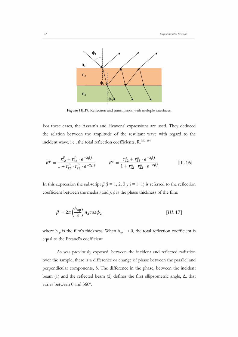
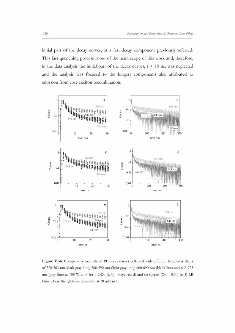
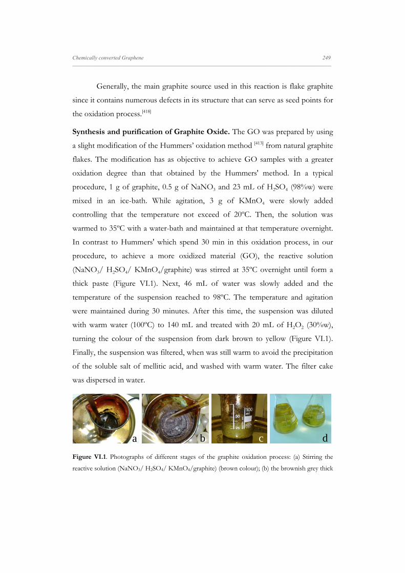
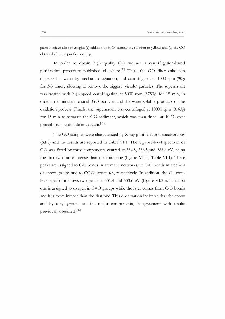
pyridine (PVP)[61]; or poly N-isopropyl acrylamide (NIPAM) [62]. Thus, the surface-
active nature of hydrophilic block promotes its spontaneous adsorption at the air-
water interface, although above a critical two-dimensional (2D) overlap density,
the solubility of this block causes it to become easily detached from the interface
and dissolved in the aqueous subphase. In order to combat this effect, the
hydrophobic block is required together the hydrophilic blocks to the surface
above the critical surface density.[41]
In addition, monolayers of polymeric surface features obtained by self-
assembly at the air-water interface can be easily transferred by the Langmuir-
Blodgett (LB) method to various solid substrates for potential applications. The
surface features obtained from LB films depend on factors such as the nature
(amphiphility, solubility, molecular weight, block ratio) of the blocks, surface
pressure, pH, temperature and concentration of the spreading solution.[63] For
example, the ionization of repeating units in block copolymers by changing the
pH or adding electrolytes in subphase, produces changes in the interfacial
behaviour an morphologies of Langmuir monolayers, precursors of the LB films.
I.2. Self-assembly of Nanoparticles at the Air-Water Interface
Self-assembly of nanoparticles is becoming a leading methodology in
fabrication of functional materials with unique optical, electronic, chemical, and
biological properties.[51, 64] In nanoparticle self-assembled structures, each
individual nanoparticle is the fundamental building-block that serves for
constructing the ordered structure. The understanding of the size- and shape-
dependent properties of individual nanoparticles, and the collective properties of
assemblies is interesting for their applications.[7]
State of the Art 13 _____________________________________________________________________________________________________________________
Focusing on the semiconductor nanoparticles, the most important factor
on their self-assembly is the organic ligands that are attached to its inorganic core
surface. Various organic ligands are used, such as phosphine oxides, phosphanes,
alkyl thiols, amines and carboxylic acids, and they drive the self-assembly of the
nanoparticles at the air-water interface. The controlled assembly of
semiconducting NPs into two-dimensional (2D) structures is a critical step toward
their use as functional elements in new materials because collective properties and
function are governed by nanoparticle organization on a combination of length
scales.[8, 65, 66] The air-water interface, and concretely the Langmuir monolayers,
provide a system that allows the manipulation of the nanoparticles and their
transfer to LB films.[67-69]
Moreover, the self-assembly of nanoparticles at the air-water interface can
be controlled by adding free excess of surfactant or amphiphilic block copolymer
molecules. The interfacial self-assembly of the mixed components leads to
different aggregates from which obtained from either pure components. Thus, it
is proposed as a technique that prevents the 3D aggregate formation and could
help to drive the 2D self-assembly process of the nanoparticles.[67, 70] The
formation of these new features is directed by the balance of interactions between
the molecules added and the nanoparticles’ ligands. [3, 14] This synergistic self-
assembly strategy results in highly stable hybrid surface features.[3] Moreover, the
better understanding of the interactions’ role is a key to build these systems.
In addition, in the case of block copolymers, self-assembly strategies offer
additional possibilities for tuning the mechanical, optical, electronic, magnetic and
catalytic properties of new nanostructured composites.[14, 71] In this case, the
different nature of the hydrophobic interaction between blocks of the copolymer
and the nanoparticle ligands directs the self-assembly of each component.[3, 14]
14 State of the Art _____________________________________________________________________________________________________________________
I.3. Self-assembly of Carbon Allotropes at the Air-Water
Interface
From fullerenes to carbon nanotubes, the ability of the air-water interface
has been demonstrated to build thin films of carbon derivatives. In the case of the
fullerenes, C60 not only form stable monolayers but also tend to 3D aggregates.
Therefore, two strategies were proposed: to use functionalized C60, that presents
amphiphilic character; and to mix C60 with a film-forming agent as surfactants or
polymers.[72, 73] On the other hand, for the single-wall carbon nanotubes (SWNTs)
the air-water interface is presented as a means that allows tube orientation and
thickness control.[74]
At present, it is the moment of the graphene-sheet derivatives.[75] Oxide
and partially reduced oxide few-layer thick graphene are viewed as unconventional
soft-materials, concretely, as 2D membrane-like colloids. Moreover, from a
scientific and technological point of view it is important to know how these thin
sheets assemble and how they behave when interacting which each other.[76] In this
type of colloid there are two kind of interactions: face-to-face (π-stacking) and
edge-to-edge. The last one controls the 2D self-assembly due to the electrostatic
repulsion promoted by the residual oxidation groups at the edges, mainly
carboxylic acid groups. Therefore, the air-water interface is suggested as an ideal
platform to investigate these interactions.[76]
II. A General Overview
A General Overview 15 _____________________________________________________________________________________________________________________
II. A General Overview
In this chapter some of the most important properties of the Langmuir
monolayers and Langmuir-Blodgett films formed by surfactants, polymers or
other soft materials are summarized. Langmuir monolayers are defined as films
formed by spreading of surface active molecules, such as surfactant, polymer or
other materials, on the clean aqueous interface without exchange of material
between the monolayer and the subphase.
II.1. Langmuir Monolayers
Langmuir monolayers are known since the Babylonians, 18th century B.C.,
who used them as form of divination based on pouring oil on water (or water on
oil) and observing the subsequent spreading. A thousand years later, this practice
was adopted by the Greeks.[77] However, the first recognized technical application
of the monolayers was in the ancient art of Japanese marbling, known as
suminagashi. This art has its origin in China over 2000 years ago, although the
Japanese began to practise it in the 12th century, converting a divinatory purpose
in an art. The technique consists of the application, on an aqueous surface, of an
ink-drop and so on other drop that disperses the other. They are blown across to
form delicate swirls, after which the image (network) was picked up by laying a
sheet of paper or silk on the ink-covered water surface.[78, 79
The first scientific investigation was made by Benjamin Franklin, in 1774,
who observed that when a small amount of oil is deposited on a water pond, the
oil spreads on the all surface.[80] However, was Lord Rayleigh, in the 19th century,
the first to carry out measurements of surface tension in olive oil monolayers
spread on water, and on from the area-density measurements, he estimated the
thickness of the oil film to be 16 Å.[81] During the following year, Agnes Pockels
made a systematic compression studies of oil monolayers on an aqueous subphase
by compressing layers with "barriers", in a "primitive" Langmuir trough, thus
16 A General Overview _____________________________________________________________________________________________________________________
observing that the surface tension fell rapidly when the monolayer was
compressed below a certain "area".[82] Later, Lord Rayleigh explained this
phenomenon by supposing that the oil molecules form a monomolecular film,
and that at this area the oil molecules were closely packed.[83] In 1917, Irving
Langmuir began to study interfaces of chemically pure substances and put
forward evidence for the monomolecular nature of the film as well as the
orientation of the molecules at the air-water interface.[84] A few years later,
Katharine Blodgett, working joined to Langmuir, showed that these monolayers
could be transferred onto solid substrates[85], and also carried out the sequential
transfer of monolayers onto the solid substrate to form multilayer films [86], which
are now referred to as Langmuir-Blodgett films.
Langmuir monolayers are formed from insoluble or a little soluble
amphiphilic molecules, as surfactants or polymers, by material deposition on the
interface, in which, there is not material exchange between the interface and the
liquid that supports the monolayer (subphase), that is usually water. Because of it,
it is possible to establish a relation between the surface concentration, Γ, and the
occupied area, A, according to the following expression:
1Γ
II. 1
Thus, from the expression, a reduction of the available area produces an
increase in the surface concentration. Therefore, by compression experiences
(area reduction), the material density deposited on the monolayer can be increased
finding a great variety of aggregation bi-dimensional states similar to the states
that exist in three-dimensions (3D).
In a monolayer the surface pressure, π, is related to the 3D pressure, P.
The surface pressure is a pressure distributed over the film thickness of the spread
material in the monolayer, Δℓ, that is usually around several nanometres.
A General Overview 17 _____________________________________________________________________________________________________________________
⁄Δℓ
2⁄ II. 2
The surface pressure, , is defined as the difference between the surface
tension of the pure liquid subphase, γ0, and the surface tension when the surface is
covered by a monolayer of adsorbed material, γ : .
The basic technique used in the study of the insoluble monolayers is the
Langmuir trough, that allows the measurement of the surface pressure as a
function of the available area at constant temperature. In this way, the Langmuir
isotherms can be obtained by compression, and in which the different states or
even surface aggregates have been reported.[1, 87]
In the case of materials of low molecular weight, the isotherm π-A can
present different quasi-bidimensional states when the available area decreases.
Some regions of phase coexistence can be observed in the Langmuir isotherms.
However, not all the isotherms present these regions. The position and the width
of them depend on the material and temperature.[87] Not all the phase transitions
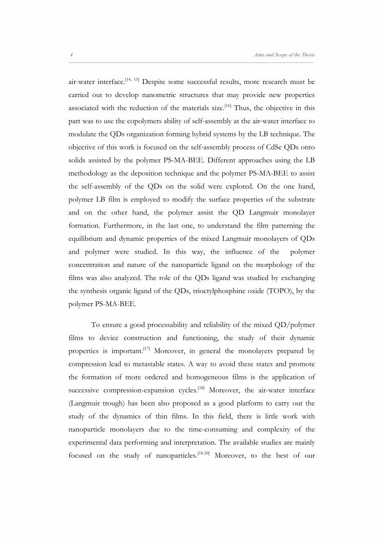
are presented in all the isotherms. Figure II.1. shows an ideal isotherm in which
are represented the majority of the possible surface states and some coexistence
regions.
18 A General Overview _____________________________________________________________________________________________________________________
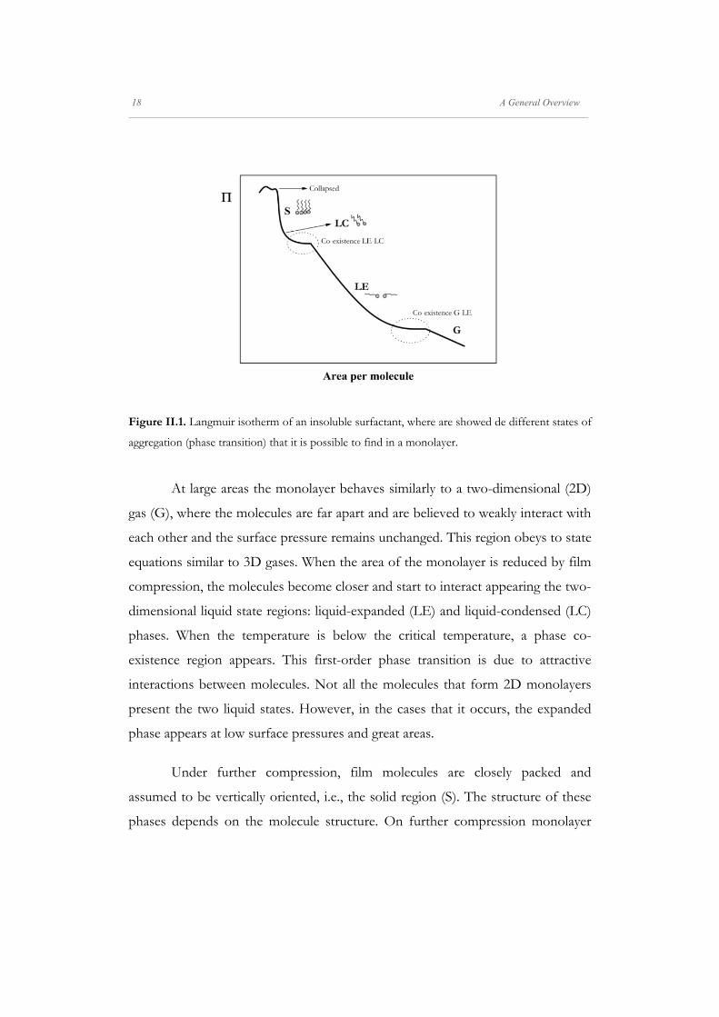
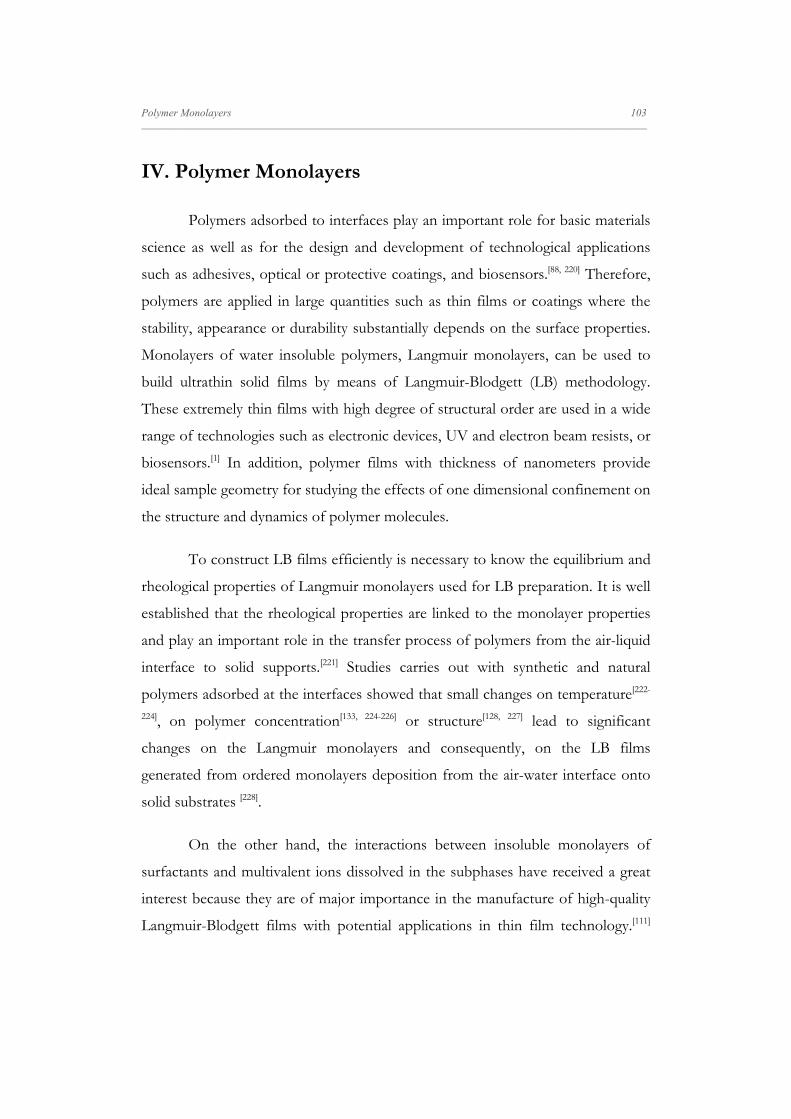
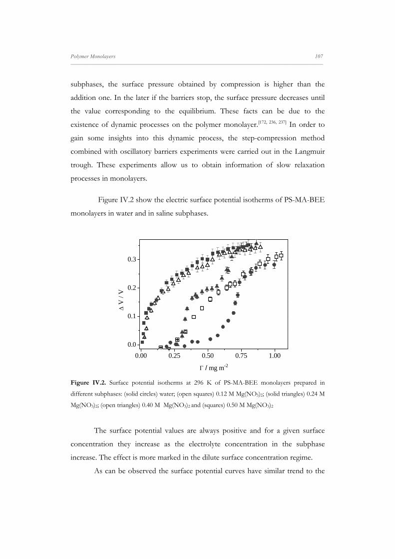
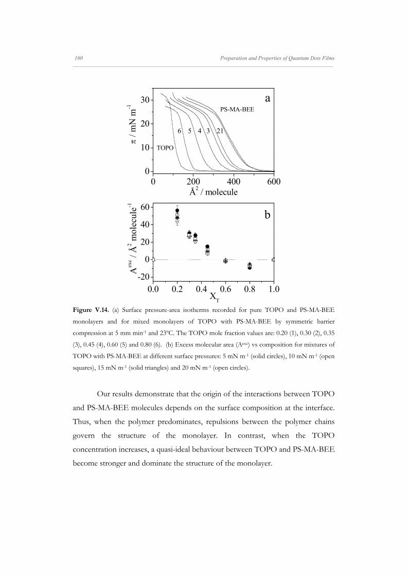
Figure II.1. Langmuir isotherm of an insoluble surfactant, where are showed de different states of
aggregation (phase transition) that it is possible to find in a monolayer.
At large areas the monolayer behaves similarly to a two-dimensional (2D)
gas (G), where the molecules are far apart and are believed to weakly interact with
each other and the surface pressure remains unchanged. This region obeys to state
equations similar to 3D gases. When the area of the monolayer is reduced by film
compression, the molecules become closer and start to interact appearing the two-
dimensional liquid state regions: liquid-expanded (LE) and liquid-condensed (LC)
phases. When the temperature is below the critical temperature, a phase co-
existence region appears. This first-order phase transition is due to attractive
interactions between molecules. Not all the molecules that form 2D monolayers
present the two liquid states. However, in the cases that it occurs, the expanded
phase appears at low surface pressures and great areas.
Under further compression, film molecules are closely packed and
assumed to be vertically oriented, i.e., the solid region (S). The structure of these
phases depends on the molecule structure. On further compression monolayer
A General Overview 19 _____________________________________________________________________________________________________________________
collapse occurs, and multilayers and non-homogeneous three-dimensional (3D)
structures are formed.[88]
The morphology of the isotherm, π-A, is influenced by many factors
including the experimental conditions and the chemical structure of the molecule.
Only the molecules that posses at least 12 carbon atoms can form an insoluble
Langmuir monolayer. The increasing of the number of carbon atoms leads to the
appearance of a great variety of liquid [89] and solid [90] phases. The polarity of the
molecule's head group also modifies its interaction with the aqueous subphase,
influencing the arrangements and the shape of the isotherm.[91]
The main properties that produce great changes in the structure of the
monolayers are: pH, the presence of ions in the aqueous subphase and the
temperature. The subphase pH mainly affects when the monolayer corresponds to
molecules with ionizable head groups, such as -COOH or -NH2.[87] In some cases,
when the head groups are completely ionized, the molecules at the interface are
dissolved in water subphase and the monolayer becomes instable. The effect of
the monolayer solubilisation in the subphase is the shift toward lower molecular
areas in comparison to the isotherm recorded for uncharged molecules, i.e,
obtaining more expanded isotherms. Therefore, in these cases it is necessary to
work at the subphase pH in which the ionisable groups are in its non-ionized
form.[92]
The addition of electrolytes in the subphase plays a critical role in the
stability of the monolayers. This effect is more accentuated in the case of
multivalent ions. The complexation of metal ions with the acid group of
amphiphiles generally causes isotherms more condensed.[93] Divalent metal ions
interact with the acid group (-COOH) in different ways, depending on their
electronegativity: the ions with high electronegativity interact covalently while
those with lower electronegativity interact electrostatically. The origin of the
interaction affects the alkyl chains packing.[94]
20 A General Overview _____________________________________________________________________________________________________________________
On the other hand, phase transitions are strongly influenced by the
subphase temperature, thus, when the temperature increases the co-existence
phase regions are shifted to higher pressures and they can disappear at sufficiently
high temperatures.[95]
One of the most important factor that affects the morphology of the
compression isotherm is the stability of the monolayer. To check the stability of
the monolayer, the surface pressure is registered during a period of time at
constant area after a barrier-compression.[96] In some cases, the monolayer does
not reach the equilibrium during the compression process, because it requires
some time after to reach the equilibrium state. In these cases after the
compression with the barriers stops the surface pressure evolves to the
equilibrium value, and when this value is reached, it remains constant. An
alternative method to check the monolayer stability is to prepare the monolayer by
addition, deposition method. Using this methodology the surface the density of
adsorbed molecules is modified by successive addition of the surfactant spreading
solution. After waiting time to solvent evaporation, the surface tension is
measured until it reaches a constant value. By comparing the surface pressure
values reached by two methods one may be able to infer on the stability of the
monolayer. Poor monolayer stability can be associated with slow material
dissolution into the subphase. However, aggregation or dynamic processes can be
responsible for differences between the surface pressure values obtained by both
methodologies.
Another way of checking monolayer stability is by performing hysteresis
experiments, where the monolayer is compressed to a fixed surface pressure or
area and subsequently expanded to the original state. Even for stable monolayers,
some hysteresis is normally observed, which is attributed either to differences
between the organization and disorganization processes or to the formation of
irreversible domains during compression process. For poorly stable monolayers,
A General Overview 21 _____________________________________________________________________________________________________________________
by applying consecutive compression-expansion cycles, usually a continuous shift
is observed in consecutive isotherms towards lower mean molecular areas.[97]
When aggregates are formed the domain size often depends on the initial surface
pressure of the monolayer.[98]
To gain insight into the states of the monolayers, the values of the
equilibrium elasticity modulus, which is the reciprocal of compressibility (CS), are
widely used:
II. 3
A useful method for classification of the monolayer phase is to examine the values
of equilibrium elasticity modulus, such dependencies are also of help in detecting
the phase transition, which appears as a characteristic minimum in the
compression modulus vs. surface pressure plots.[99]
II.2. Mixed Langmuir Monolayers
Mixed monolayers formed by co-spreading two different compounds have
important application in the formation of functional LB films. Thus, mixed
monolayers are an option adopted in many cases to improve monolayer stability [100, 101] and the film properties [102]. Mixed monolayers have also been useful for
constructing LB films with interlocking structures[103] and improving the
orientational order of molecules in films [104]. One of the most important aspect to
use accurately mixed monolayers is to study both the miscibility and the
interactions between the components. The methodology widely used to study the
interactions between components is to analyse the composition dependence of
the mean area per molecule (A12) expressed as [99]:
II. 4
22 A General Overview _____________________________________________________________________________________________________________________
Where A1, A2 are the molecular areas of single component at the same surface
pressure and X1, X2 are the mole fractions of components 1 and 2 in mixed films.
The way mean molecular areas depend on the composition of the mixture can be
used to infer possible interactions in the mixed monolayer. Thus, if two
components are ideally miscible or immiscible, A12 linearly depends on the
monolayer composition.[105-107] Deviations of this behaviour indicate attractive or
repulsive interactions between components.[108] In order to analyse the nature of
interactions between the components, the excess area of mixing (Aexc) defined as:
II. 5
is usually employed. Accordingly, positive Aexc values, positive deviation from the
ideal mixing, indicate repulsive interaction between components. While negative
values are signature of attractive interactions between them.[99, 109] However, it is
often difficult to obtain homogeneous and ordered mixed LB films, because
phase separation of the components is often observed. The mixed monolayers
and transferred multilayers generally give heterogeneous structures with small
domains of each component.[87]
II.3. Langmuir-Blodgett Films
As it has been mentioned above, Katherine Blodgett joined to Irving
Langmuir, was the first person able to transfer fatty acid monolayers from the air-
water interface onto solid substrates, forming as-called Langmuir-Blodgett (LB)
films.[85] The objective was to transfer, assemble and manipulate simple films,
previously prepared at the air-water interface. Since then, the possibilities that
offer this technique have increased due to the necessity of organized systems
construction by controlling the assembly of monolayers looking for the
development of molecular machines.[110] Nowadays, the LB technique is an useful
tool to build self-assembled systems with applications in several areas of the
Nanotechnology and in the development of new electronic and optoelectronic
devices.[1, 111]
A General Overview 23 _____________________________________________________________________________________________________________________
The LB method consists in placing a solid substrate on a support
perpendicularly to the air-water interface covered by the monolayer that will be
transferred by immersion or emersion of the solid. During the transfer process
the surface pressure is kept constant by barrier compression in order to
compensate the loss of molecules transferred onto the solid.
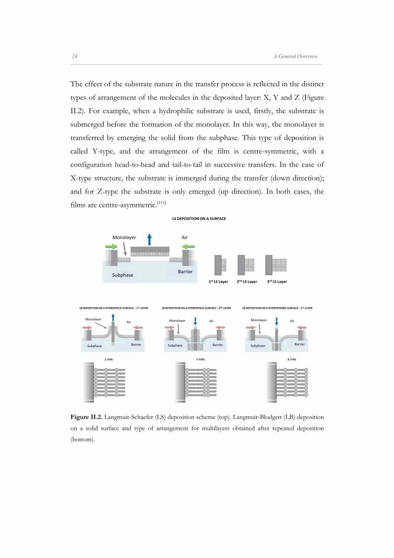
One variant of this methodology is the horizontal deposition technique,
named as Langmuir-Schaefer (LS) technique.[112] In this method, the solid
substrate, placed parallel to the air-water interface, is made to contact with the
surface of the monolayer. In other words, the deposition is done by dipping the
substrate horizontally through a floating monolayer from the gas phase (air)
toward the liquid phase (monolayer). In this way, the monolayer is transferred
with the hydrophobic part on the solid and the polar head in contact with the air.
Another possibility is the Kossi-Leblanc technique, where the substrate is placed
inclined with regard to the air-water interface, usually with an angle of 40º, and
then is submerged on the subphase. The transfer occurs by dipping up the
support as in the LB deposition.[113]
The understanding of the physicochemical phenomena (mechanisms) that
control the LB transfer are still understudy.[114, 115] The molecular interactions
involved in the air-water interface can be different than the interactions at the air-
solid interface. When the monolayer is transferred from the air-water interface
onto the solid the interface changes, and therefore, in the majority of the cases the
monolayer structure is not kept. Because of it, the construction of high quality
LB films requires a high degree of skill joined to a careful control of all the
experimental parameters, such as: stability and homogeneity of the monolayer;
subphase properties (composition, pH, presence of electrolytes and temperature);
substrate nature (structure and hydrophilic or hydrophobic character); solid speed
of immersion/emersion; angle of the substrate with the interface; surface pressure
during the deposition process; and number of transferred monolayers.[111]
24 A General Overview _____________________________________________________________________________________________________________________
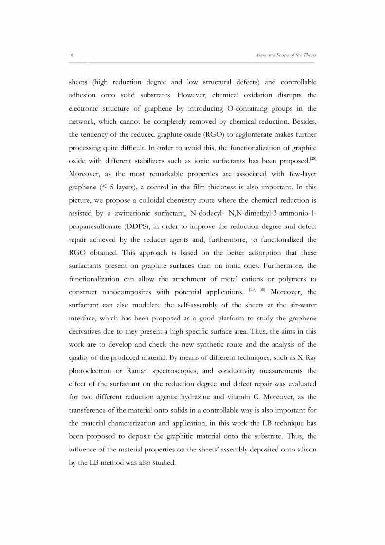
The effect of the substrate nature in the transfer process is reflected in the distinct
types of arrangement of the molecules in the deposited layer: X, Y and Z (Figure
II.2). For example, when a hydrophilic substrate is used, firstly, the substrate is
submerged before the formation of the monolayer. In this way, the monolayer is
transferred by emerging the solid from the subphase. This type of deposition is
called Y-type, and the arrangement of the film is centre-symmetric, with a
configuration head-to-head and tail-to-tail in successive transfers. In the case of
X-type structure, the substrate is immerged during the transfer (down direction);
and for Z-type the substrate is only emerged (up direction). In both cases, the
on a solid surface and type of arrangement for multilayers obtained after repeated deposition
(bottom).
LS DEPOSITION ON A SURFACE
SubphaseBarrier
AirMonolayer
1st LS Layer 2nd LS Layer 3rd LS Layer
Z‐TYPE Y‐TYPE X‐TYPE
Subphase Barrier Subphase BarrierBarrierSubphase
Air AirMonolayer Monolayer AirMonolayer
LB DEPOSITION ON A HYDROPHILIC SURFACE – 2ND LAYER LB DEPOSITION ON A HYDROPHOBIC SURFACE – 1ST LAYERLB DEPOSITION ON A HYDROPHILIC SURFACE – 1ST LAYER
A General Overview 25 _____________________________________________________________________________________________________________________
In the LB films, the molecular arrangement is not as perfect as in the
theoretical schemes. As it has been well established in a number of experiments,
the properties of transferred LB films may differ from those of the corresponding
Langmuir films, even for simple model amphiphilic molecules. This is not
unexpected, since the factors governing the equilibrium packing arrangement of
the molecules in Langmuir and LB films are presumably different. The molecules
can reorganize during or immediately after transfer to a more stable arrangement
on a solid support. A typical example is the observation of transition from a X-
type to a Y-type LB film during monolayer transfer, usually explained in terms of
an over-turning mechanism (detach-turnover-reattach) when the film is inside the
subphase water.[116] Moreover, several forces act during the dewetting promoting
the drying-mediated self-assemblies.[69]
A comparison between Langmuir and Langmuir-Blodgett films is still
possible, nevertheless, particularly if one accounts for the change of interface and
possibility of molecular over-turning due to processes such as dewetting [44, 45] that
occurs at the air-solid interface. However, there are some parameters such as level
of mixing between components in a mixed monolayer and the composition of the
monolayer and the degree of ionization of head groups, which can conveniently
be assumed as unchanged during the transfer process if there is no specific
interaction between the monolayer material and the substrate.[79]
After the construction of the LB films it is important to study the
architecture and organization of the molecules in order to establish the theoretical
molecular models in films: molecular orientation or interactions. For this purpose,
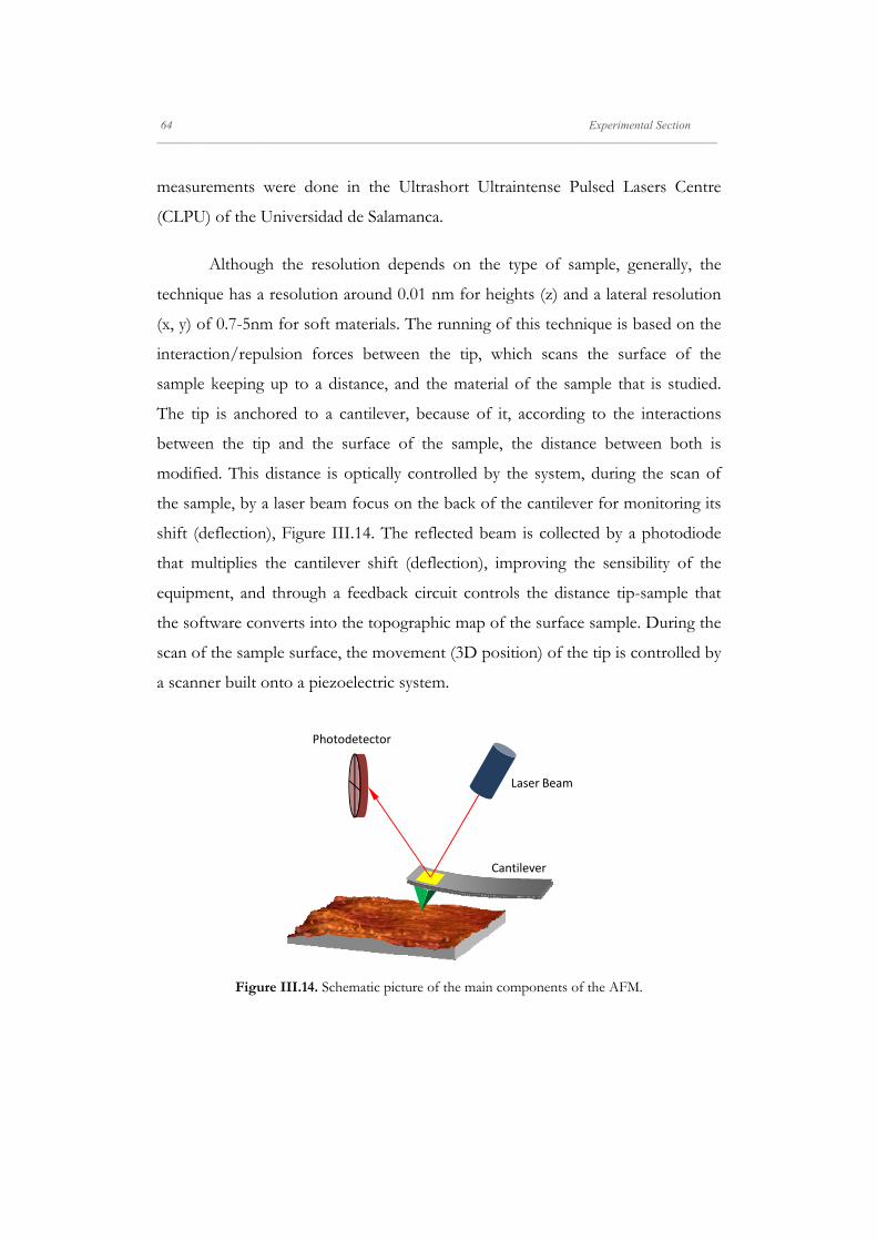
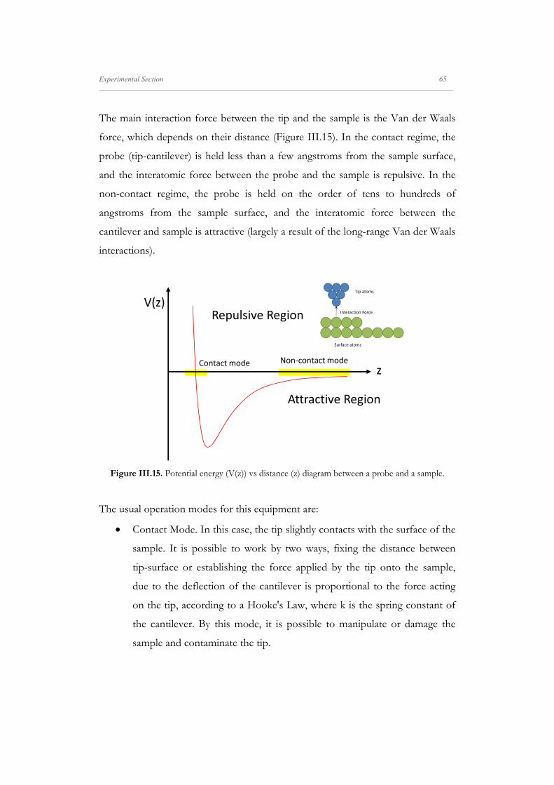
complementary techniques such as atomic force microscopy, transmission and
scanning electronic microscopy, ellipsometry and UV-vis, IR or Raman
spectroscopy, give information about the density of the adsorbed molecules,
structure, morphology and composition of the film [117], respectively.
26 A General Overview _____________________________________________________________________________________________________________________
II.4. Polymer Langmuir Monolayers
The study of insoluble monolayers constituted by polymers is important in
the basic material science and in several technological applications such as
adhesion, colloids stabilization and coatings. Polymers spread at the air-water
interface can be viewed as pseudo-two-dimensional systems of fundamental
interest for studying the effects of one-dimensional confinement on the structure
and dynamics of polymer molecules. On the other hand, polymer thin films are
relevant in the development of electronic devices or different kind of sensors
whose characteristics depend on the surface properties. It is necessary to
emphasize that despite the amount of studies in this matter, several questions in
the polymer systems spread at interfaces are not yet well understood.[118]
As in the case of polymers in solution, in the structure of adsorbed
polymers influence not only the concentration but also their interaction with the
subphase. For polymers in solution it is possible to establish several concentration
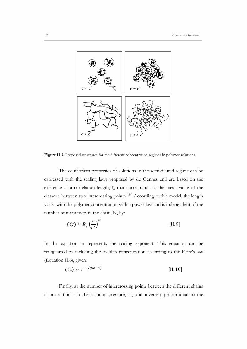
regimes, Figure II.3. Dilute solutions, where the polymer concentration is low
enough that the chains do not interact. If the polymer concentration increases and
the overlap concentration, c*, is reached the polymer chains began to interact
forming a network where solvent molecules are present, i.e., in semi-dilute
solutions. Thus, according with the interactions polymer-solvent, it is possible to
differentiate three behaviours: good-solvent, θ-solvent and poor-solvent. For
good-solvent conditions the polymer chains do not interpenetrate and are mixed
with the solvent. There is a repulsive potential between the chains due to the
volume excluded effect. At poor-solvent conditions there is a repulsive interaction
polymer-solvent, so the polymer conformation is closed in order to expulse the
solvent molecules. In the θ-solvent conditions, there are not interactions polymer-
solvent and the polymer chains are in a non-perturbed situation.
A General Overview 27 _____________________________________________________________________________________________________________________
In these systems the scaling-laws are applied [119] to predict the polymer-
interface behaviour. The overlap concentration, c*, is a parameter that allows us to
determine the polymeric chain radius of gyration (Rg, or Flory's radius) and the
solvent quality by:
∗~ II. 6
Where, N is the number of monomers in the chain, and d, the spatial
dimensionality (in two-dimension d = 2). Besides, the radius of gyration [120, 121] is
related to the number of monomers in the chain by the following expression:
~ II. 7
Where ν, is the Flory's scaling exponent, that is a measurement of the polymer-
solvent interactions and whose value depends on the dimensionality, d:
32
II. 8
Finally, when the polymer concentration reaches the double-overlap
concentration, i.e, in concentrated solutions, the chains are very closed and
consequently, there is low solvent content between the chains, lead to a semi-
crystalline, glassy or melt state.
28 A General Overview _____________________________________________________________________________________________________________________
Figure II.3. Proposed structures for the different concentration regimes in polymer solutions.
The equilibrium properties of solutions in the semi-diluted regime can be
expressed with the scaling laws proposed by de Gennes and are based on the
existence of a correlation length, ξ, that corresponds to the mean value of the
distance between two intercrossing points.[119] According to this model, the length
varies with the polymer concentration with a power-law and is independent of the
number of monomers in the chain, N, by:
∗ II. 9
In the equation m represents the scaling exponent. This equation can be
reorganized by including the overlap concentration according to the Flory's law
(Equation II.6), given:
⁄ II. 10
Finally, as the number of intercrossing points between the different chains
is proportional to the osmotic pressure, Π, and inversely proportional to the
c > c* c >> c*
c < c* c ~ c*
A General Overview 29 _____________________________________________________________________________________________________________________
intercrossing distance, ξ, the scaling law can be expressed for the osmotic pressure
as below:
Π~ ~ ⁄ II. 11
In order to establish the different states of the polymer molecules at the
monolayer, it is usual to apply the polymer in solution concentration regimes by
analogy with 3D polymer solution. Accordingly, it is possible to differentiate three
regimes in the polymer isotherms. The diluted regime where the surface pressure
slowly increases with the surface concentration. The semi-diluted region, that
begins at the overlap concentration (Γ*), in which the pressure increases quickly,
and the concentrated region. This region corresponds to the monolayer collapse
leading to 3D structures.
Spread polymer films do not show the variety isotherm behaviour as that
for compounds of low relative molecular weight. Depending on the isotherm
morphology, generally, two types are observed: liquid expanded and condensed
films.[88] In the expanded monolayers the increasing of surface pressure with the
concentration is less than in the condensed monolayers, Figure II.4. The surface
pressure isotherms for polymers are usually represented in terms of the surface
concentration (Γ), because the relative molecular weight of polymers is generally
not an unique value.
30 A General Overview _____________________________________________________________________________________________________________________
Figure II.4. Schematic surface pressure isotherms of the two major types encountered in spread
polymer films.
As it was mentioned, the surface property widely used to characterize the
polymer monolayers state at the interface, is the equilibrium elasticity, ε0, obtained
from the surface pressure isotherm [122]:
ΓΓ
II. 12
The equilibrium elasticity is related to the response of the monolayer to a
deformation and gives information about its conformational state. Thus, values
below 20 mN m-1 correspond to high disorder conformations that lead to high
flexibility states, while values above this value correspond to very rigid
conformations as in the case of condensed polymer random-coils.[88] In this sense,
the different states of the monolayer are characterized by the equilibrium elasticity
values as follows: liquid expanded states show values between 12.5 and 50 mN m-
1; liquid condensed films varying between 100 and 250 mN m-1; and solid
condensed states present values from 1000 to 2000 mN m-1. [123, 124]
A General Overview 31 _____________________________________________________________________________________________________________________
Generally, the equilibrium properties of adsorbed polymers in the semi-
dilute regime were interpreted by the scaling laws adapted to two-dimensional
systems.[125] However, it is not clear the validity of Flory scaling exponent in 2D,
because the theory of polymer solutions is based upon the existence of
entanglements between polymer chains and the existence of entanglements in
polymer quasi-2D systems is still a matter of controversy.[126-128]
The models for polymer in solution were later adapted to two-dimensional
systems, d=2. In this case the polymer concentration represents the polymer
surface concentration, Γ. Accordingly, the scaling law for polymeric monolayers
can be expressed as follows [129]:
Γ ~Γ II. 13
And for the surface pressure, π:
~Γ II. 14
The rheological properties of monolayers play an important role to predict
the behaviour of thin layers in technological processes, such as the transference of
polymer monolayers onto solid substrates, or natural processes, as the rheological
behaviour of lung surfactant responsible for facilitating breathing. Even thought
the rheological properties of monolayers have received great attention, the
physical mechanism involved in the dynamics of polymer chains at interfaces is
still a challenge.[130, 131]
The monolayers are subjected to external perturbations that originate
different kinds of movement or reorganization processes, therefore it is necessary
to know the dynamic properties. In order to study these phenomena, the
interfacial rheology is used. The basic methodology consists in producing a
deformation and studying the system response, i.e., the monolayer response.
32 A General Overview _____________________________________________________________________________________________________________________
From the relation between the amplitudes of the response and deformation is
used to obtain information about the processes involved in the deformation. In
the case of Langmuir monolayers, one resorts to mechanical deformations in the
Langmuir trough. The mechanical deformation can be carried out by two ways:
sudden step-compression/expansion or sinusoidal oscillatory experiments. These
experiments are in the frequency range of 1mHz-1 Hz. This low frequency causes
slow collective movements in the monolayer, accordingly, the information
obtained is related to these movements.[130]
The results available for polymer monolayers show that they present a
complex dynamics and the results can be interpreted from the models for
polymers in solution in the semi-dilute regime.[125, 132, 133]
II.5. Langmuir Monolayers of Nanoparticles
In recent years, nanoparticles have received much attention due to their
great potential to be used in biological and technological applications. This
possibility is related to their size dependent optical, electric and/or magnetic
properties.
The studies on nanoparticle materials at the air-water interface are relied
on traditional amphiphilic molecules. The nanoparticles (NPs) have a polar core
with a hydrophilic or hydrophobic surface. Consequently, the hydrophobic NPs
serve as the surface-active molecules to build a Langmuir monolayer, while the
hydrophilic ones can be dispersed in the aqueous subphase and incorporated to
the monolayer by attractive interactions with amphiphilic molecules adsorbed on
the air-water interface. Thus, the hydrophobic NPs form themselves the
Langmuir monolayer while the hydrophilic ones need additives. An alternative
method to obtain hydrophobic NPs from the hydrophilic ones is by capping alkyl
chains on the particle surfaces, either by via chemical grafting [134-136] or by physical
adsorption[137-139].
A General Overview 33 _____________________________________________________________________________________________________________________
Focus the attention on hydrophobic NPs, the surface pressure-area
isotherms of their monolayers present a characteristic behaviour. Thus, they
display a first transition plateau at negligible surface pressure. In this region, the
NPs are probably clustered as small islands floating on the subphase. A steep rise
in surface pressure follows as the islands begin to touch. The islands merge to
form a monolayer which can withstand surface pressures up to 65 mN m-1 before
collapsing.[140] Moreover, on hydrophobic NPs, ligand-ligand interactions play a
decisive role in the monolayers assembly and dynamics behaviour. For example,
shorter ligands lead to a more densely packed monolayers. In this sense, other
important factors that influence the NPs monolayer properties are: particle size[140,
141], material composition, nature of surface stabilizing molecules, and surrounding
environment [67]. In fact, the monolayer behaviour and quality have been reported
to be strongly dependent on the degree of surface hydrophobic character, as well
as the capping method used. Therefore, when such particles are spread at the air-
water interface, the weak particle-water interaction results in the formation of void
defects or 3D aggregates in the monolayer.[139, 142, 143] A possible solution is to
modulate the hydrophobic character by using mixed systems.
Besides, the π-A isotherms other measurements that are carried out in
these systems at the air-water interface to gain insight about the changes in the
film during compression, are the surface potential and the rheological properties.
Concerning to surface potential measurements, they allow to obtain information
about film morphology. At larger areas, the NPs are randomly distributed at the
air–water interface and as result, the total surface potential contribution is zero.
The film can be compressed with minimum particle–particle interactions. When
the monolayer is further compressed, the hydrophobic part of the NPs began to
stretch out of the water and the change of the dipole moment resulted in a rapid
increase of surface potential corresponding to the lifting point of the surface
pressure. The monolayer is in a state similar to a liquid condensed phase where
the NPs started to interact among them. From this point, a slight increase of the
34 A General Overview _____________________________________________________________________________________________________________________
surface potential was observed although the change of surface pressure was still
significant. This may be due to the reorientation of the NPs in order to maximize
the exposure of hydrophobic ligand moiety to the air. The maximum of the
surface potential corresponds to the solid phase region of the isotherm. At this
solid phase region of the isotherm, the surface potential curve changed its
slope.[139]
Moreover, mixed systems have been proposed with NPs, concretely, two
approach have been developed in mixed monolayers with NPs. One methodology
widely used is based on the mixture of different kind or size NPs to form
complex architectures [69] called superlattices. Multicomponent NPs superlattices
are proposed to create multifunctional materials by combining independently
tailored functional components.[9] Another option is the addition of a surfactant [67, 144-149] or polymer [14, 15, 148, 150] excess or even co-mixtures [151] in order to control
the NPs assemblage and can be also used to develop hybrid materials [9]. The
thermodynamic treatment of these mixed monolayers is similar to amphiphilic
molecules mixtures. The study of the mixed monolayers is based on the average
area and collapse pressure values behaviour. Thus, a non-linear area trend suggests
that the self-assembly of the two components is synergistic in nature, thus, the
presence of one component influences the surface conformation of the other.[150]
As in the case of amphiphilic mixed monolayers, the collapse pressure variation
with composition is other parameter to highlight the two-component miscibility.
Thus, if the NPs collapse pressure is maintained almost constant, the two
components of the mixed monolayer are immiscible and there is minimum
interdigitation among the NPs ligand and the co-spread molecules. However, a
change in the collapse surface pressure can be a result of miscibility and
interdigitation of the two components at the interface.[145]
The field of the dynamic properties of NPs monolayers at the air-water
interface is largely unexplored although is very remarkable for their
A General Overview 35 _____________________________________________________________________________________________________________________
applications.[152] In spite of their relevance, there is little detailed work in the
literature [19-21] and mainly focused on NP films without co-additives due to only
the understanding of the dynamical NPs behaviour requires a very complex study.
The first observation in the dynamic properties of NPs monolayers is the
hysteresis that their isotherms presents [70, 143, 145], indicating that the films are rigid
and interparticle interactions at the air-water interface are attractive [140, 143, 153]. The
hysteresis behaviour is also explained in terms of a low re-spreading ability of NPs
or a slow expansion rate of the NPs.[145] The overcompression cycles annealing the
NP monolayer structures so that the monolayer defects disappear. This is due to
the increase of the long and short-range order induced by the ligands converging
towards a homogeneous interdigitation fraction and compensating for NP core
size inhomogeneities.[18] Accordingly, there is a lot of interest to study the dynamic
properties in the case of NPs layer at the air-water interface, because is a good
methodology to self-assembly NPs in an ordered and homogeneous way.
However, one of the difficulties encountered with measurements on particle
monolayers is that they are solid-like, non-zero shear modulus, and the standard
data analysis is no longer valid. To illustrate this picture, in the rheological studies,
relaxation measurements and continuous or oscillatory deformations are carried
out by means of barrier movements in a Langmuir trough. In these experiments,
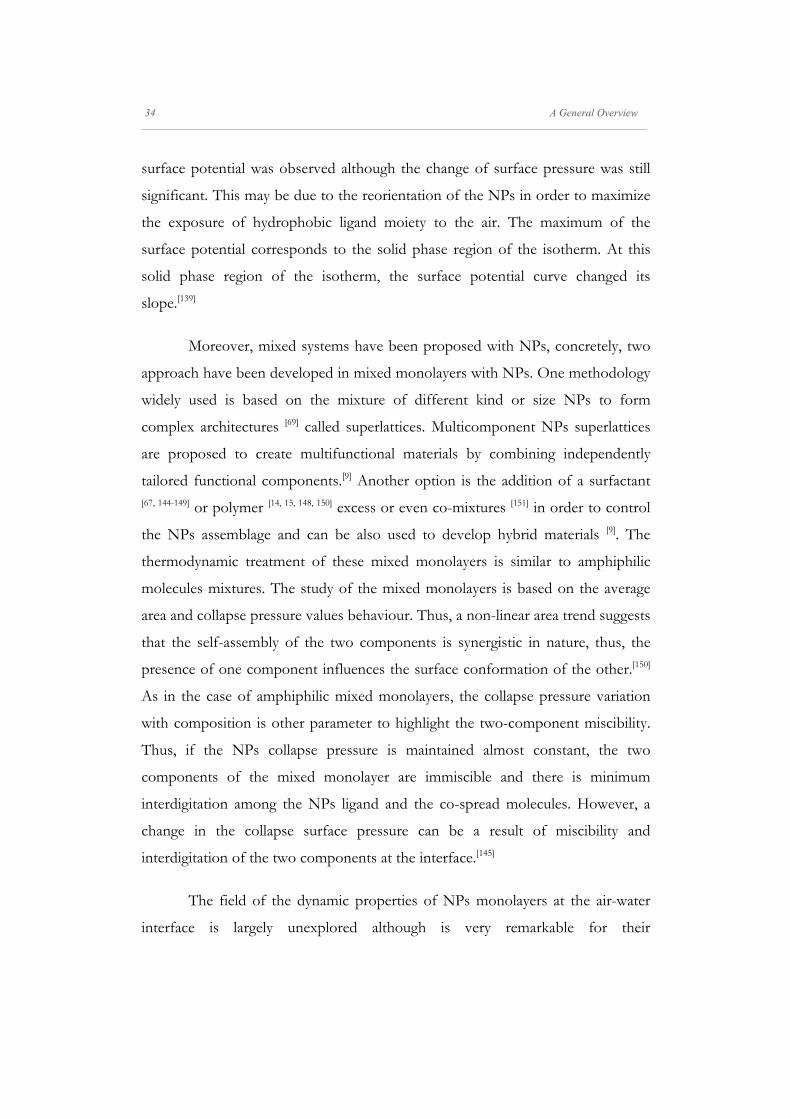
one observation is the surface pressure anisotropy effect. The effect consists in
measuring the different increase with compression of the surface pressure in the
perpendicular and parallel compression (push) direction for NP monolayers. This
anisotropy occurs when the water surface is fully covered by particles and
becomes more prominent with the increase of surface concentration. This effect
reflects the non-homogeneous distribution of particles at the interface, so that the
particle distance decrease in the parallel direction is much more prominent than
that in the perpendicular direction, leading to the non-homogeneous states of
particles distribution (Figure II.5).
36 A General Overview _____________________________________________________________________________________________________________________
Figure II.5. Dynamic mechanism of the nanoparticle monolayer. The scheme shows the
evolution of the surface pressure tensor. At the initial state (equilibrium) the surface pressure is a
symmetrical tensor. Under barrier unidirectional compression, particles are more condensed in
this push-direction and the surface pressure becomes unsymmetrical. After relaxation, the
particles rearrange reaching a new equilibrium state, then the surface pressure becomes
symmetrical again. (Adapted from Zang, 2010 [154]).
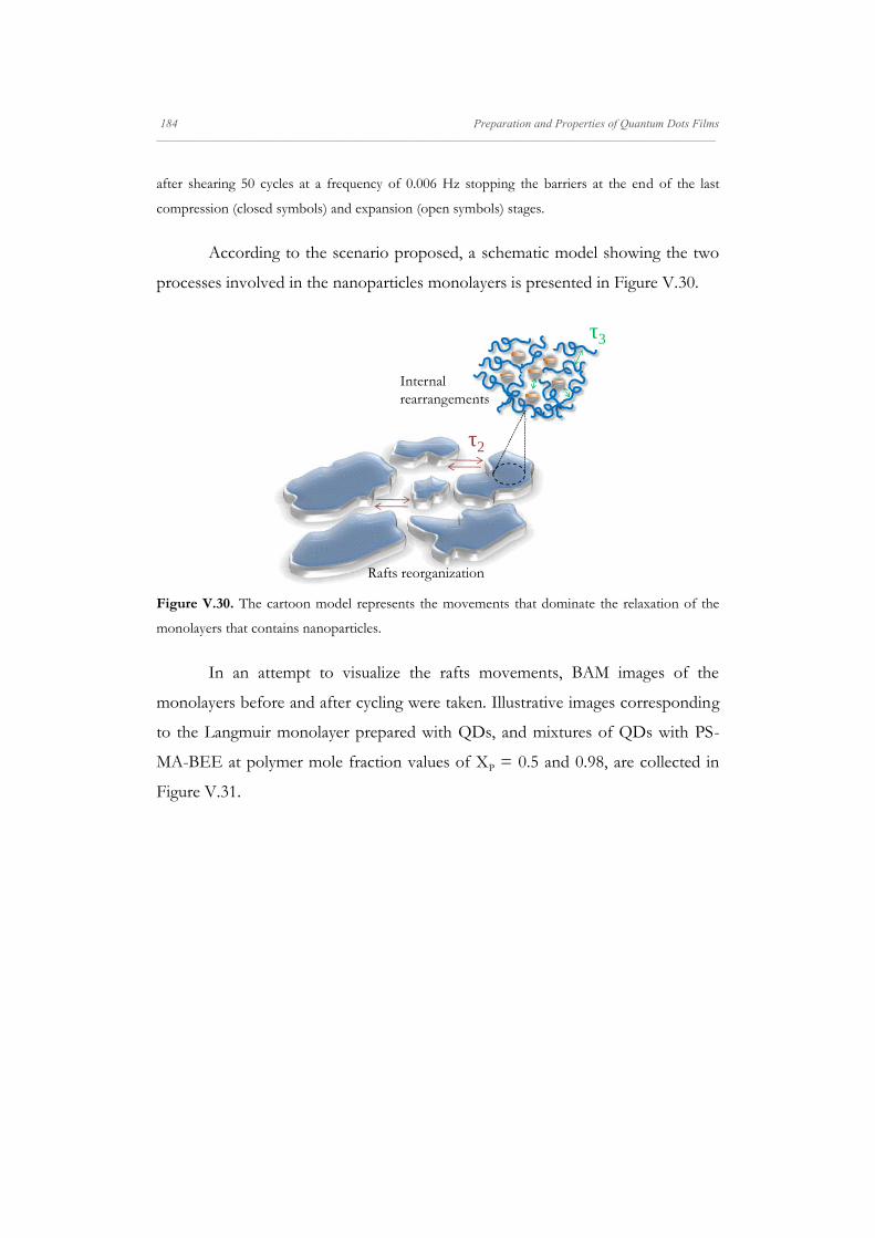
On the other hand, the NPs films present a complex relaxation of surface
pressure that involves three timescales which are related to the damping of surface
fluctuation, rearrangement of particle rafts and particle motion inside each raft.
Therefore, the particle layer posses a long relaxation time and a fast compression
brings the particle layer to a non-equilibrium state. While under oscillation,
additional energy is provided to the layer. This accelerates the decay dynamics
remarkably and the suppression of surface pressure decay. With the increase of
oscillation time, surface pressure response amplitude decays exponentially and
eventually reaches the equilibrium value. Upon long term barrier oscillation, the
particle aggregates organize parallel to the barrier and respond collectively to
compression.[20, 154]
Finally, recent dynamic studies have been carried out with NP/surfactant
mixed monolayers to evaluate the effect of NPs on the surfactant monolayer
properties. These investigations have important implications on technological
applications or biological studies such as modeling respiratory cycles in the
presence of particle pollutants with lung surfactants.[21, 155] The results point out
π//π ⱵPO
PO P
OP
O
PO
PO
POP
O
P O
PO
PO
P
O PO
PO
PO
PO
POP
O
P O
PO
PO
PO P
OP
O
PO
PO
POP
O
P O
PO
PO
P
O PO
PO
PO
PO
POP
O
P O
PO
PO
PO P
OP
O
PO
PO
POP
O
P O
PO PO
PO P
OP
O
PO
PO
POP
O
P O
PO
Initial state Barriers compression Relaxation
π//
π Ⱶ
Surface Pressure tensor components evolution
A General Overview 37 _____________________________________________________________________________________________________________________
that the presence of NPs induces significant changes in both the phase behaviour
and the dynamic response of surfactant monolayers due to the reduction of the
available area to the surfactant molecules at the interface and to the disruption of
the interfacial structure of the monolayer caused by the incorporation of the NPs.
Significant differences in the interfacial properties of these mixed systems have
been evidenced depending on the NP surface nature and concentration.[21, 155]
II.6. Langmuir Monolayers of Graphene Derivatives
From the graphene work performed by K. Novoselov and A. Geim in
2004, the graphene and its derivatives have extraordinary re-emerged and become
very important from a fundamental and applied point. Their excellent mechanical
and electrical properties favour their use in technologic and biological applications
such as the construction of solar cells, batteries and biosensors.[156] However, the
challenge is the graphene large scale production. In this way, the chemical routes
are one of the most promising approaches due to are cheap, processable and
scalable methods, although the graphene material obtained presents slightly
inferior properties than pristine graphene.[157] These approaches are based on the
oxidation of carbon materials obtaining graphene oxide and its subsequent
reduction to reduced graphene oxide. By continuing with this way, different liquid
phase exfoliation methods have been developed to produce dispersions of
graphene or graphene oxide sheets.[158] However, the next challenge to implement
the graphene is how to transfer the sheets formed from the dispersion onto a
substrate in a controlled manner at variable coverage on an arbitrary surface.[159]
Moreover, for practical application or simply for fundamental research purposes,
a good adhesion and an uniform and reproducible deposition of graphene to the
substrate is of great importance. Thus, recently Langmuir-Blodgett (LB) [75, 160] and
Langmuir-Schaefer (LS) deposition[159, 161] have shown promising results in
preparing graphene layers with high degree of control and under ambient
38 A General Overview _____________________________________________________________________________________________________________________
conditions in contrast to other techniques such as spin-coating [162] or drop
casting[163].
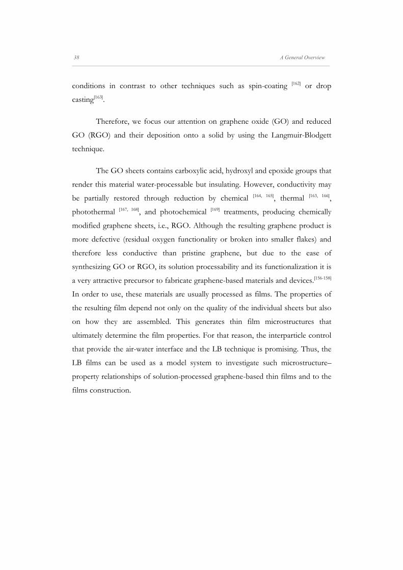
Therefore, we focus our attention on graphene oxide (GO) and reduced
GO (RGO) and their deposition onto a solid by using the Langmuir-Blodgett
technique.
The GO sheets contains carboxylic acid, hydroxyl and epoxide groups that
render this material water-processable but insulating. However, conductivity may
be partially restored through reduction by chemical [164, 165], thermal [163, 166],
photothermal [167, 168], and photochemical [169] treatments, producing chemically
modified graphene sheets, i.e., RGO. Although the resulting graphene product is
more defective (residual oxygen functionality or broken into smaller flakes) and
therefore less conductive than pristine graphene, but due to the ease of
synthesizing GO or RGO, its solution processability and its functionalization it is
a very attractive precursor to fabricate graphene-based materials and devices.[156-158]
In order to use, these materials are usually processed as films. The properties of
the resulting film depend not only on the quality of the individual sheets but also
on how they are assembled. This generates thin film microstructures that
ultimately determine the film properties. For that reason, the interparticle control
that provide the air-water interface and the LB technique is promising. Thus, the
LB films can be used as a model system to investigate such microstructure–
property relationships of solution-processed graphene-based thin films and to the
films construction.
A General Overview 39 _____________________________________________________________________________________________________________________
Scheme II.1. Chemical structures of the different graphene materials: graphene oxide (GO),
reduced graphene oxide (RGO) and pure graphene. The structures were calculated by molecular
mechanics, MM2, with the Chem 3D Ultra 9.0. software.
GO sheets can be considered amphiphilic with an edge-to-center
distribution of hydrophilic and hydrophobic domains. The edges of GO are
hydrophilic due to the ionizable -COOH groups, while its basal plane contains
many poly-aromatic islands of unoxidized graphene nanodomains that provides
hydrophobic character. Thus, GO can adhere to interfaces and lower interfacial
energy, acting as a surfactant. Due to its surface activity, it is possible to employ
molecular assembly methods as the Langmuir-Blodgett technique to create
monolayers in order to process the GO with a precise control over film thickness.
To spread GO at the air-water interface it is necessary to use a solvent.
Though typical spreading solvents are volatile and water-immiscible (e.g.,
chloroform, toluene), these solvents do not disperse GO well.[170] Since GO is
amphiphilic, it can be spread from alcohols that are even miscible with water, such
as methanol.[76] When methanol droplets are gently dropped on water surface, it
can first spread rapidly on the surface before mixing with water. In this way, the
GO surfactant sheets can be effectively trapped at the air–water interface. The
density of sheets can then be continuously tuned by moving the barriers and the
packing is controlled by the surface pressure. At zero surface pressure, the film
consists of dilute, well-isolated flat sheets. As compression continues, a gradual
increase in surface pressure begins to occur and the sheets start to close pack. If
GO RGOGraphene
40 A General Overview _____________________________________________________________________________________________________________________
the compression continues, the soft sheets are forced to fold and wrinkle at their
edges. This behaviour at the collapse region is different than the 3D aggregation
observed for surfactants or polymers. A technique used to observe the GO
assembly at the air-water interface is the Brewster angle microscopy (BAM). The
GO sheets are visible due to their large lateral dimension and optical contrast.
However, BAM imaging of a freshly prepared GO dispersion revealed little
material on the surface. This can be attributed to the different GO sheets
solubility on water. In this way, the large sheets are less hydrophilic and can float
on the water surface while small, more oxidized are more hydrophilic sheets and
therefore, sink into the subphase. Therefore, as the GO dispersion is usually
polydisperse, the water surface itself, without any features, can be used as a size-
separation method for GO sheets.[171] A way to minimize the GO sheets sinking is
to bubble a gas in the subphase. Thus, the process can be controlled by bubbling
air or nitrogen where the surface active sheets adhere to rising gas bubbles and
become trapped upon reaching the water surface.[160] When these monolayers are
transferred onto a solid, the LB assembly produces flat GO thin films with
uniform and continuously tunable coverage, thus avoiding the uncontrollable
wrinkles, overlaps, and voids in films fabricated by other techniques such as dip-
coating, spin coating, drop casting, etc.[156, 158]
In opposite of GO, the RGO has a more hydrophobic character due to
after the reduction step some oxygen groups are reduced. Accordingly, the RGO
sheets can be firstly dispersed and then spread at the air-water interface using
organic solvents such as 1,2-dichloroethane [75] or dimethylformamide [161] and can
float more easily. With respect to the RGO sheets, their packing behaviour
response to barrier compression and LB deposition process are similar to the GO.
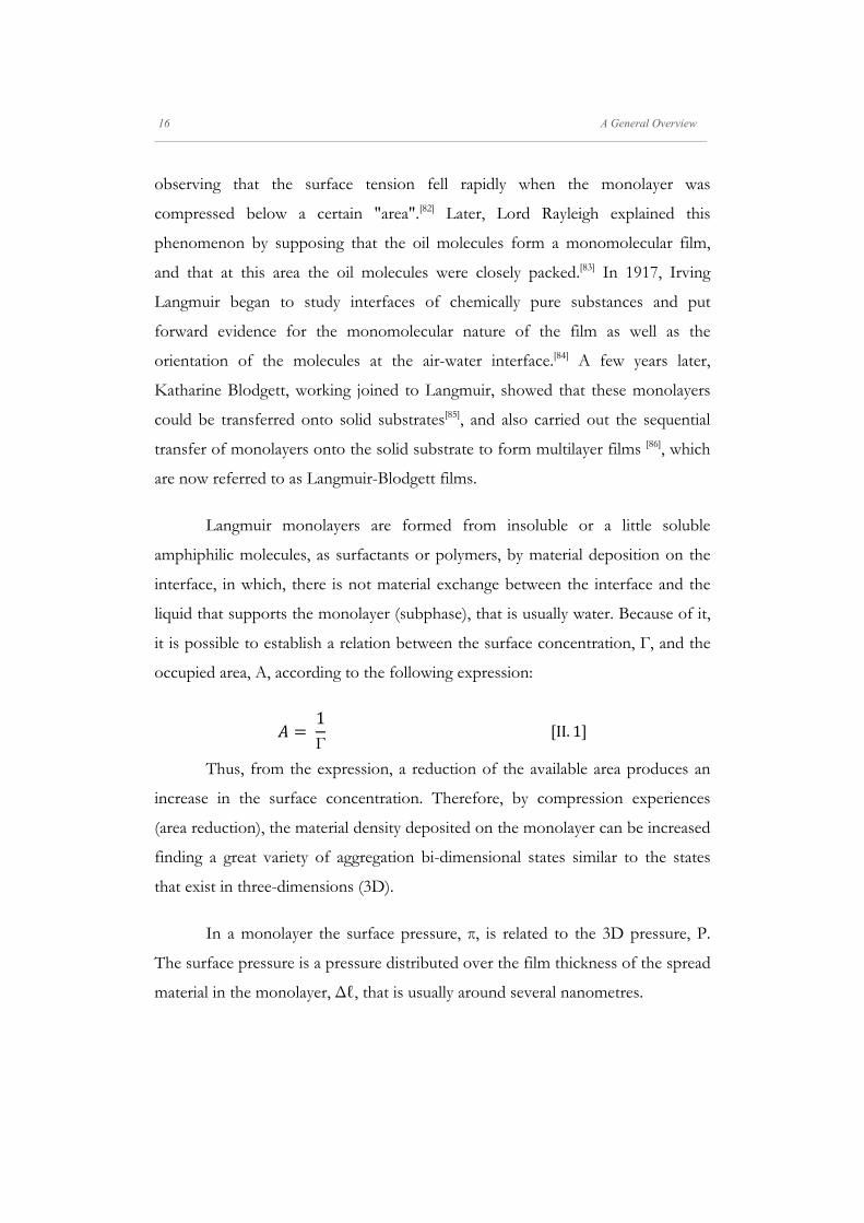
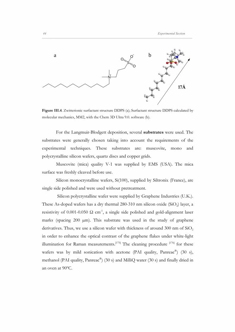
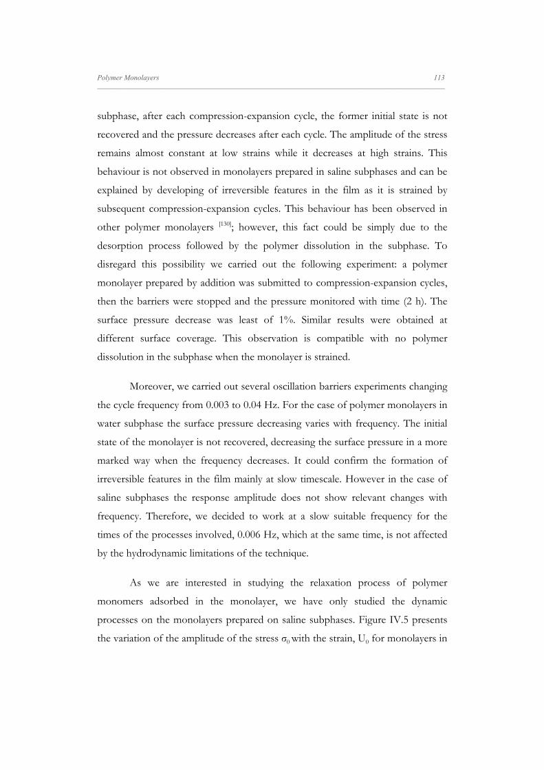
Figure IV.16. Elasticity modulus (a) and dilatational viscosity (b) variation with oscillatory
frequency for PS-b-MA monolayers on water subphase at 293K (squares) and 307K (circles).
Oscillatory barrier experiments were carried out at 10% strain and at a polymer surface
concentration of 1 mg m-2.
0.003 0.006 0.009 0.012 0.015 0.01860
65
70
75
Fluid-like
mod
ulus
/ m
N m
-1
/ Hz
Solid-like
0.003 0.006 0.009 0.012 0.015 0.0180
2000
4000
6000
8000
10000
0.005 0.01 0.015 0.02
1000
10000
/ m
N s
m-1
/ Hz
/ m
N s
m-1
/ Hz
a b
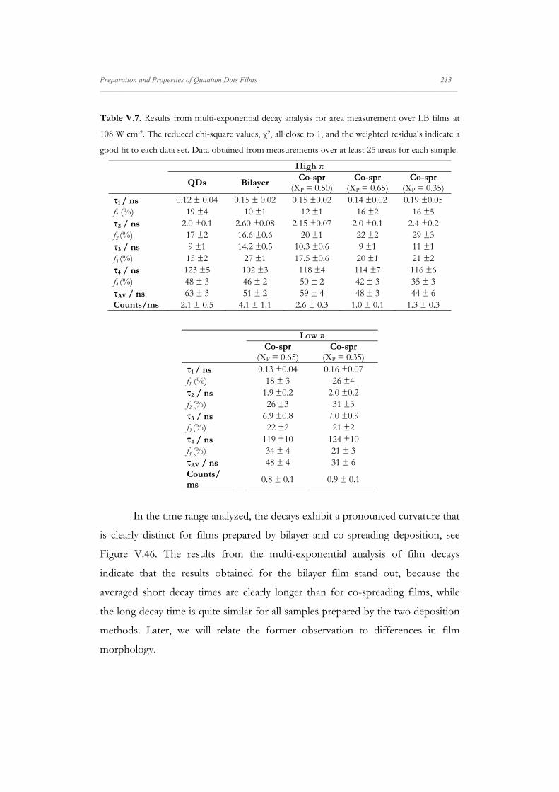
V. Preparation and Properties of QDs Films
Preparation and Properties of Quantum Dots Films 133 _____________________________________________________________________________________________________________________
V. Preparation and Properties of QDs Films
Semiconductor quantum dots (QDs) have attracted much attention in
recent years owing to their unique chemical and physical properties [7] and their
applications as building blocks for photovoltaic,[254, 255] optoelectronic[256] or
magnetic devices,[257] and for selective recognition of ions[258] or biomedical
applications[259]. Inside the QDs, the hydrophobic nanoparticles present higher
quantum efficiency than the hydrophilic ones.[260] The current interest in the
fabrication of nanodevices is focused on the incorporation of QDs in well defined
layers and their immobilization onto solid substrates to obtain good quality
devices.[37, 51] In this sense the interfacial self-assembly is a selective method to
provide well-organized structures with controlled size and shape for the
fabrication of optoelectronic devices with QDs.
Moreover, the nanoparticle-polymer blend systems have shown potential
applications based on the modulation of the hybrid material properties to achieve
significant enhancements.[8] However, many nanofillers used in nanocomposites
tend to agglomerate by attractive interactions[153, 261] decreasing the quality of
nanocomposites. Therefore, the most recent efforts involve the use of polymer or
surfactant molecules to minimize filler agglomeration. Despite the great interest
aroused in the last years, more work must be carried out to develop
multifunctional materials with novel electric, magnetic or optical properties.[63, 262,
263]
An important issue concerning the properties of filler deposited on solids is
to achieve control over the organization and assembly of nanoparticles at
interfaces. Many techniques have been used to achieve good-quality
nanocomposites.[264-266] For hydrophobic nanoparticles an effective method to
produce well-defined QDs monolayers could be the Langmuir-Blodgett technique
(LB). The LB methodology (LB) has been proposed as a platform that renders the
self-assembly process of different hydrophobic nanomaterials at the air-water
134 Preparation and Properties of Quantum Dots Films _____________________________________________________________________________________________________________________
interface under well controlled and reproducible conditions.[1, 2] Therefore, it
offers the possibility of preparing polymer and nanoparticle reproducible films
with the control of the interparticle distance necessary to exploit the
nanocomposites in technological applications. In addition, the dewetting
processes observed in the preparation of LB films can be employed to achieve
patterning without a defined template. Despite the above mentioned advantages,
when the hydrophobic nanoparticles were transferred from the air-water interface
onto glass, silicon or mica substrates without treatment to become the solid
surface hydrophobic, low coverage and nanoparticle agglomeration have been
observed in LB films.[69, 140] To solve this problem some authors have proposed
two approaches. In the first one, mixed Langmuir films of surfactants[67, 146-149] or
polymers[14, 15, 148, 267] and hydrophobic nanoparticles are transferred from the air-
water interface onto solid substrates by the LB method. This approach seeks to
control the assemblage of hydrophobic nanoparticles on water. In the case of
polymers, if the polymer is an amphiphilic block copolymer, the most hydrophilic
block can favour the nanoparticles spreading and the adsorption on the solid
avoiding the 3D aggregation. Moreover, because block copolymers can aggregate
at the interface[59, 63], the self-assembly of nanoparticles on these copolymers can
be proposed as a way to organize hybrid materials at nanometre scale[13, 267, 268]. The
second methodology proposed is the interchange of the stabilizer ligand, TOPO,
by thiols [269], alkylamines [270], alkylphosphoramines [7] and block copolymers [14, 150,
271, 272]. Even though some improvements have been achieved with this
methodology, the appropriate control of the self-assembly process remains still a
challenge. Despite the successful results reported, more efforts must be carried
out to develop nanometric structures that may provide new phenomena
associated with the size reduction of materials.[147] Thus, major advances in the
field of self-assembly must be made in order to achieve a better understanding of
the process to make use of the functionality offered by nanomaterials and to
improve their practical applications.
Preparation and Properties of Quantum Dots Films 135 _____________________________________________________________________________________________________________________
With this objective in mind, we focus our interest on the self-assembly of
CdSe QDs onto solid substrates assisted by the block copolymer PS-MA-BEE.
We choose this polymer because it self-assembly at the air-water interface at a
given polymer surface concentration.[273] Therefore, as polymer assembly modifies
the surface properties[274-277] it provides us an excellent way to study the role of the
surface properties of the precursor Langmuir monolayer on the LB film
architecture and photoluminescence properties. On the other hand,
styrene/maleic anhydride copolymers have shown potential application in optical
waveguides, electron beam resists and photodiodes.[5, 6] Therefore, it could be a
good candidate to prepare hybrid materials for optoelectronic devices
fabrication.[13, 267, 268]
To assist the QDs self-assembly, we use the polymer PS-MA-BEE in three
different ways. In the first strategy, we use the polymer as matrix to assist the
QDs self-assembly at the air-water interface. Thus, a QD/PS-MA-BEE mixed
Langmuir monolayer is transferred by the LB method onto the solid. In the
second one, a LB film constructed by the polymer PS-MA-BEE is used as coating
for the substrate to deposit the QDs Langmuir films. Here the polymer was used
in order to control the QDs adsorption on the solid. We use this polymer because
spreads well onto the substrates used. The presence of the polymer on the solid
essentially modifies the surface properties of the substrate and could allow tuning
the QDs film properties. In the third approach, the QD stabilizer, TOPO, is
exchanged by the polymer to analyze the effect of the ligand on the modulation of
self-assembly at the air-water interface. This polymer contains a free carboxylic
acid group that can interact with the Cd2+ localized in the surface of the QD
core.[8] The assemblies obtained with these QDs are transferred by the LB
methodology onto the solid wafer.
Accordingly, this chapter is organized in three parts. In the first one, we
prepare the LB films by the proposed strategies and study the different film
136 Preparation and Properties of Quantum Dots Films _____________________________________________________________________________________________________________________
morphologies by means of atomic force microscopy (AFM) and transmission
electron microscopy (TEM). Previously, we carried out the characterization of the
Langmuir monolayers which serve as precursors of the LB films by performing
the surface-pressure isotherms and by obtaining images of the monolayers using
the Brewster Angle Microscopy (BAM).
In the second part of the chapter, the dynamic properties of mixed
Langmuir films of PS-MA-BEE and QDs were studied. This part has a double
objective. On the one hand, the study of the influence of the shearing on the
QD/PS-MA-BEE film morphology and on the other hand, to analyze the
dynamic processes involved in the reorganization of the monolayers after shearing
due to the knowledge of the dynamic properties of these nanocomposites is
essential in order to guarantee the processability, reliability and stability of
QD/polymer devices.[17] In this sense, the effect of the mixture composition is
also investigated.
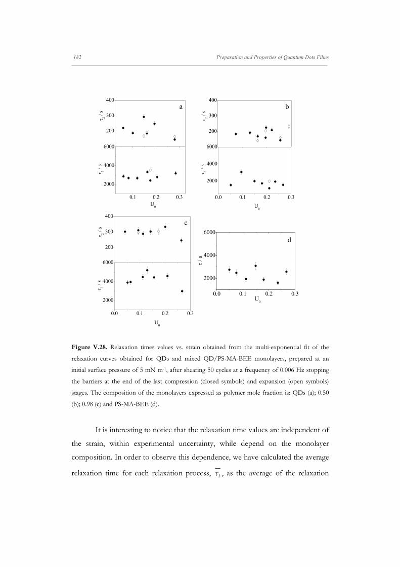
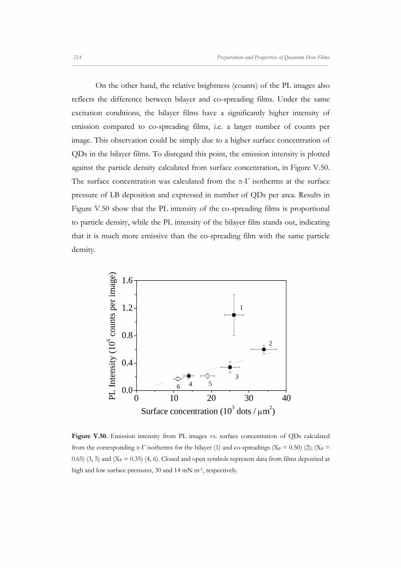
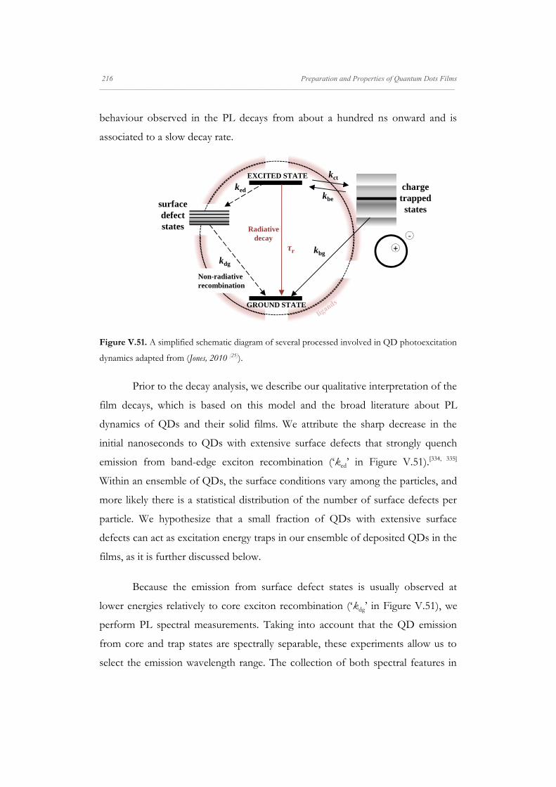
Finally, as the QDs emission can be used to fabricate LEDs, the
fluorescence properties of the QD films were studied analyzing the effect of the
self-assemblies morphology on the QD emission properties. This
photoluminescence characterization was performed by means of Fluorescence
Lifetime Imaging Microscopy (FLIM).
V.1. Experimental Section
In this section the synthesis, extraction and size characterization of the
TOPO-capped CdSe QDs used in this work is briefly presented.
The hydrophobic QDs were synthesized by the method proposed by Yu
and Peng.[278] This method uses cadmium oxide and selenium powders as
precursors. Firstly, a selenium precursor solution was prepared by mixing Se
(0.030 g), TOP (0.4 mL) and octadecene (5 mL). The solution is stirred and
Preparation and Properties of Quantum Dots Films 137 _____________________________________________________________________________________________________________________
warmed as much as necessary to speed dissolution of the Se, forming a colourless
solution of trioctylphosphine selenide (TOPSe) valid for five syntheses that was
stored at room temperature in a sealed container.
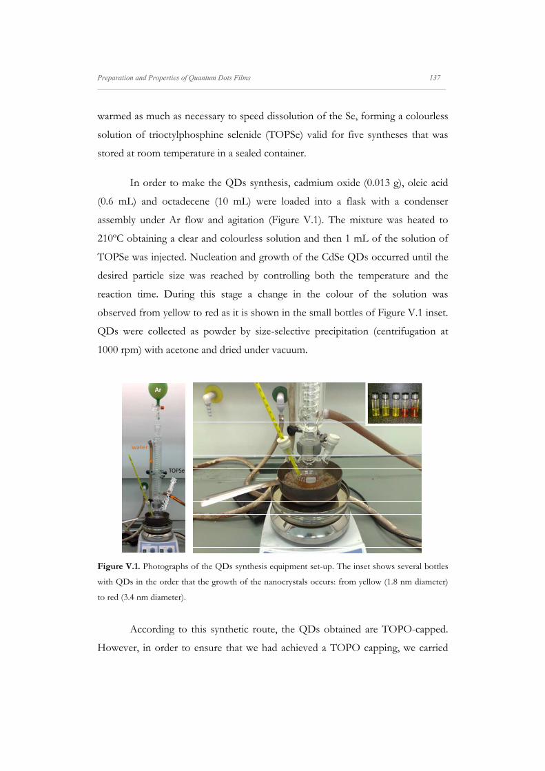
In order to make the QDs synthesis, cadmium oxide (0.013 g), oleic acid
(0.6 mL) and octadecene (10 mL) were loaded into a flask with a condenser
assembly under Ar flow and agitation (Figure V.1). The mixture was heated to
210ºC obtaining a clear and colourless solution and then 1 mL of the solution of
TOPSe was injected. Nucleation and growth of the CdSe QDs occurred until the
desired particle size was reached by controlling both the temperature and the
reaction time. During this stage a change in the colour of the solution was
observed from yellow to red as it is shown in the small bottles of Figure V.1 inset.
QDs were collected as powder by size-selective precipitation (centrifugation at
1000 rpm) with acetone and dried under vacuum.
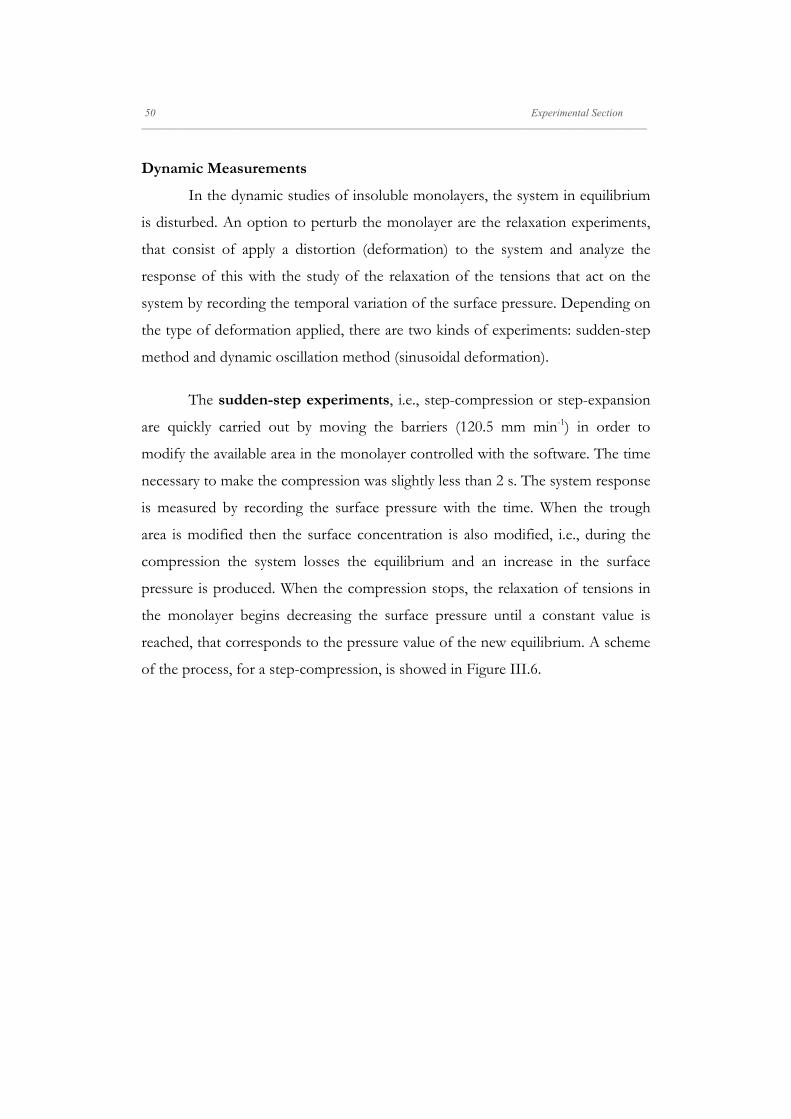
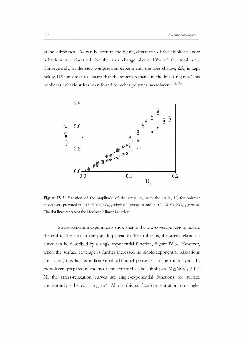
Figure V.1. Photographs of the QDs synthesis equipment set-up. The inset shows several bottles
with QDs in the order that the growth of the nanocrystals occurs: from yellow (1.8 nm diameter)
to red (3.4 nm diameter).
According to this synthetic route, the QDs obtained are TOPO-capped.
However, in order to ensure that we had achieved a TOPO capping, we carried
Ar
water
TOPSe
138 Preparation and Properties of Quantum Dots Films _____________________________________________________________________________________________________________________
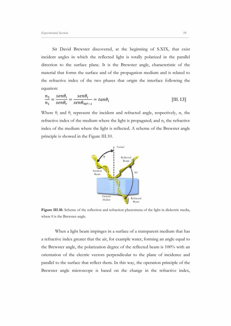
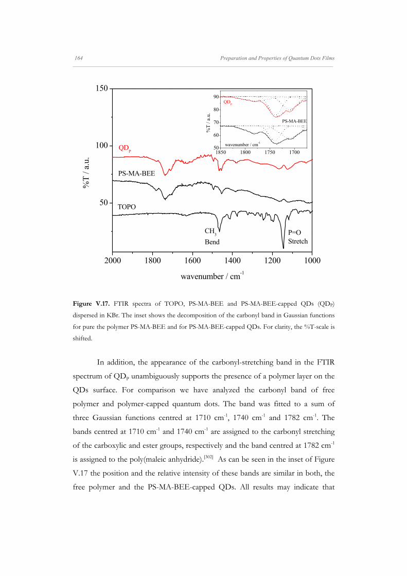
out FTIR measurements with QD powder and TOPO, Figure V.2. The FTIR
spectrum of nanoparticles presents peaks matching the TOPO spectrum, except
for the peak at 1144 cm-1 corresponding to the P=O stretch. It was demonstrated
that this peak is shifted between 20 and 60 cm-1 lower relative to bulk TOPO
upon complexation with CdSe.[279] Therefore, the peak centred at 1108 cm-1 in the
FTIR spectrum of QDs can be ascribed to the phosphonate molecules bound to
the nanoparticles surface. Thus, by comparing the QDs and TOPO FTIR spectra,
namely the P=O stretch frequency [280], we confirmed the presence of the
phosphonate ligand on the nanoparticle surface. Furthermore, latter studies
indicate that in similar syntheses [281] a thorough surface analysis reveals that the
nanoparticles are capped by octylphosphonate derivative ligands, which remain
bound to the surface (Cd2+ binding) after precipitation/washing steps.
1600 1400 1200 10000
20
40
60
80
100
CH3
Bend P-O Stretch
% T
/ a.
u.
wavenumber / cm-1
QDTOPO
TOPO
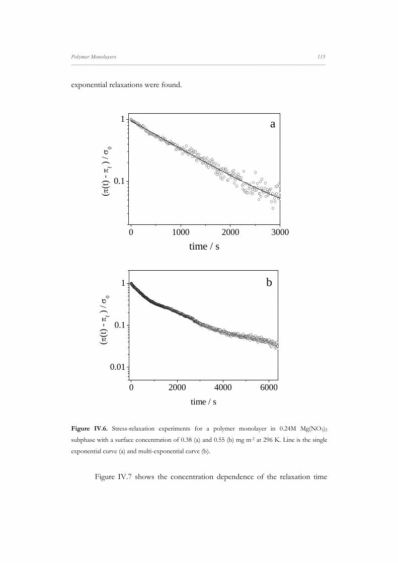
Figure V.2. FTIR spectra of TOPO and TOPO-capped QDs, (QDTOPO), dispersed in KBr. For
clarity, the %T-scale is shifted and the QDTOPO spectrum amplified.
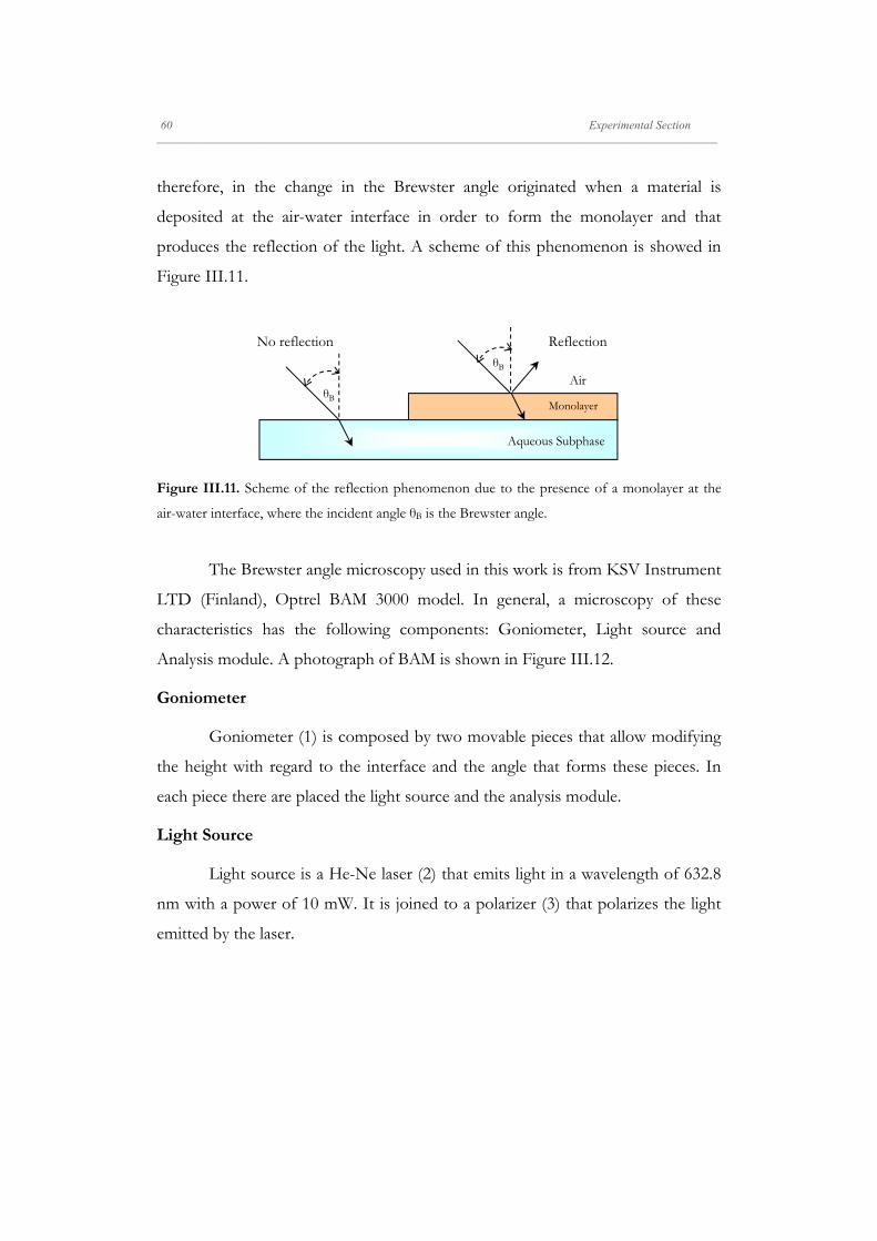
The diameter of the QDs was determined by the position of the maximum
of the visible spectrum of the QDs dispersed in chloroform [204], Figure V.3. The
Preparation and Properties of Quantum Dots Films 139 _____________________________________________________________________________________________________________________
value found was (566 ± 1 nm) that corresponds to a nanoparticle diameter of
(3.41 ± 0.05 nm), the red solution bottle in Figure V.1 inset. The QD size selected
is the most controllable size in the synthesis used as the nanocrystal growth and
population is controlled by time. Therefore, by this synthesis the maximum
diameter, ca. 4 nm, and the greatest QDs population are achieved at longer times.
The concentration of nanocrystals was calculated from the UV-Vis absorption
spectrum of the QDs solutions by using the extinction coefficient per mole of
nanocrystals at the first excitonic absorption peak.[204] UV-Vis absorption spectra
were recorded on a Shimadzu UV-2401PC spectrometer, Figure V.3.
400 500 600 700
UV
-Vis
abs
orba
nce
(a.u
.)
/ nm
3.4 nm
2.8 nm
2.2 nm
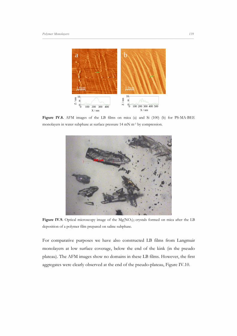
Figure V.3. Normalized absorption spectra of several CdSe QDs solutions in chloroform. The
diameter of the nanoparticles is also indicated.
V.2. Preparation of QDs Films
V.2.1. Langmuir and Langmuir-Blodgett Films of QDs and PS-MA-BEE
The first strategy employed was to use the polymer as matrix to assist the
QDs self-assembly. Therefore, we transfer mixed Langmuir monolayers of
140 Preparation and Properties of Quantum Dots Films _____________________________________________________________________________________________________________________
TOPO-capped CdSe QDs and PS-MA-BEE from the air-water interface onto
mica. As small changes on the composition of a mixed monolayer modify the
structure of the film,[172, 174, 250, 282] we study the effect of the polymer concentration
on the surface properties of the Langmuir films precursors of the LB films. The
characterization of these mixed monolayers allows us to select monolayers with
very different surface properties and to transfer them onto mica, in order to
investigate the role of these properties on both, the morphology of QDs films and
the self-assembly process.
The surface properties of the Langmuir monolayers were studied by
recording the surface pressure-concentration isotherms of the pure components
and mixtures of QDs and polymer at different composition. According to results
presented in chapter IV, the LB films obtained by transferring PS-MA-BEE
Langmuir monolayers prepared by addition consist of metastable states. Thus, we
prepare the Langmuir monolayers by compression because this method renders
the most reproducible and stable LB films in the case of the polymer. Figure V.4a
shows the isotherms of different mixtures and pure components, QDs and PS-
MA-BEE.
In the case of mixed monolayers it is well established that their surface
properties depend on the spreading technique.[172, 283, 284] Therefore, we test the
isotherm properties of monolayers obtained by spreading both components at the
interface, named as co-spreading, or adding the components separately. In all
cases the isotherms were very stable. A representative example for mixed
monolayers of polymer mole fraction XP = 0.50 is presented in Figure V.4b.
Significant differences between the isotherms can be observed. Thus, from the
three spreading procedures the densest monolayer is that obtained by co-
spreading. This behaviour was observed in other systems [172, 283] and ascribed to
the existence of attractive interactions between polymer and QDs molecules in
the spreading solution [283]. As was demonstrated in our previous work,[172, 284] the
Preparation and Properties of Quantum Dots Films 141 _____________________________________________________________________________________________________________________
co-spreading method proved to be the most reproducible technique and
consequently, was chosen to build the mixed QD/PS-MA-BEE monolayers.
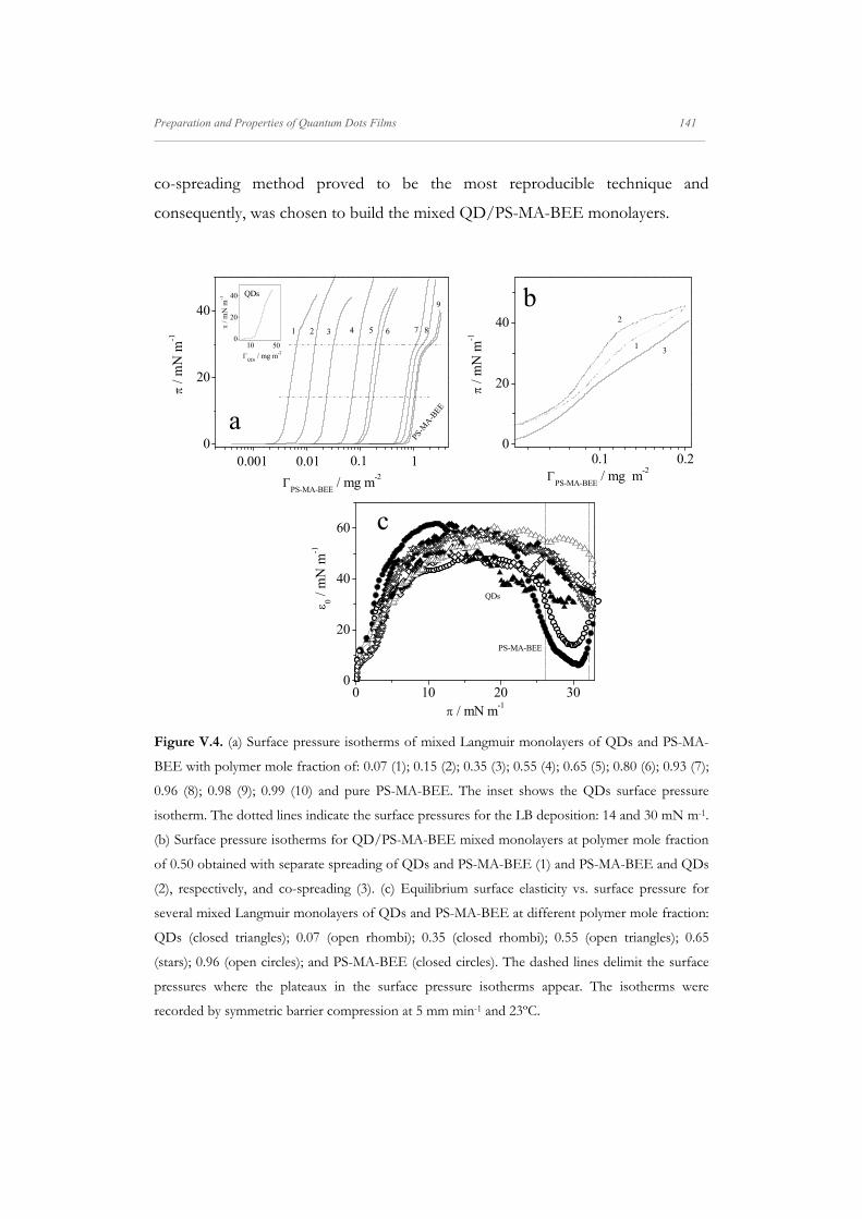
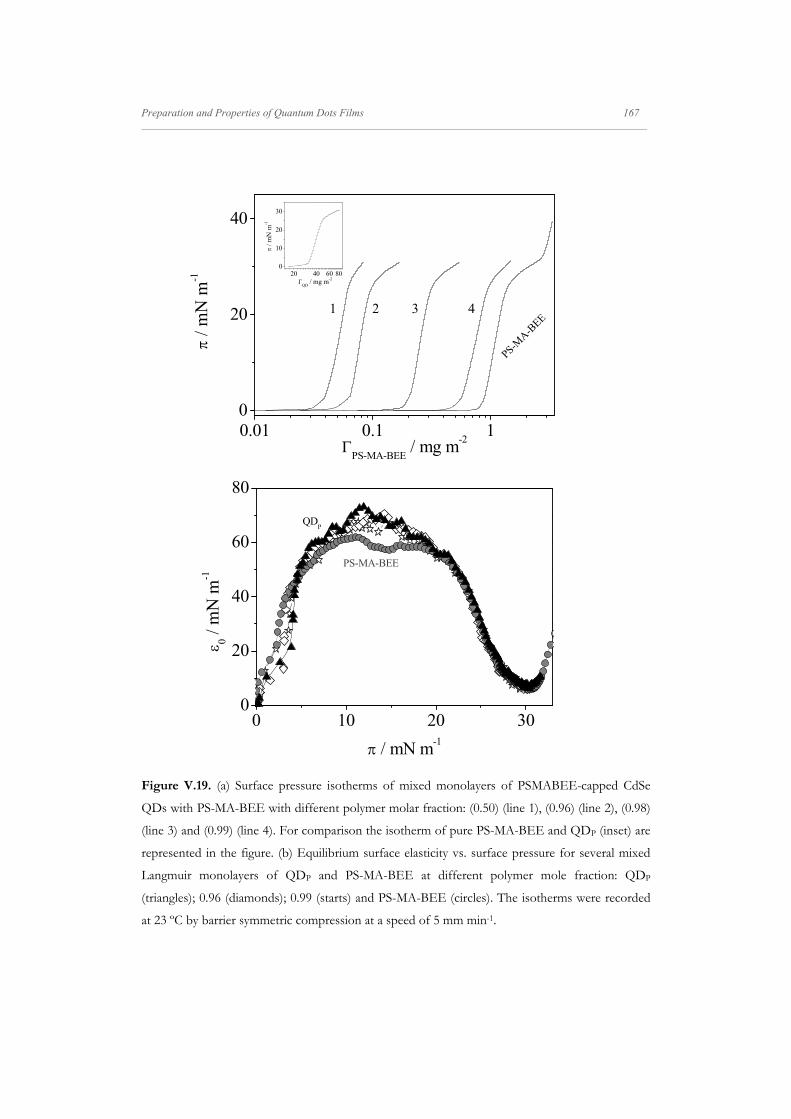
Figure V.4. (a) Surface pressure isotherms of mixed Langmuir monolayers of QDs and PS-MA-
(stars); 0.96 (open circles); and PS-MA-BEE (closed circles). The dashed lines delimit the surface
pressures where the plateaux in the surface pressure isotherms appear. The isotherms were
recorded by symmetric barrier compression at 5 mm min-1 and 23ºC.
0
20
40
10.10.001
100
20
40
/ m
N m
-1
QDs
/ mg m-2
50
9
875431 2
/ m
N m
-1
PS-MA-BEE
/ mg m-2
PS-M
A-B
EE
6
QDs
0.01 0.1 0.20
20
40
3
2
/ m
N m
-1
PS-MA-BEE / mg m-2
1
a
b
c
0 10 20 300
20
40
60
0 / m
N m
-1
/ mN m-1
PS-MA-BEE
QDs
142 Preparation and Properties of Quantum Dots Films _____________________________________________________________________________________________________________________
The QDs and PS-MA-BEE isotherms agree with those reported
previously.[67, 273] In mixed monolayers, at high polymer concentration, XP ≥ 0.95,
the isotherms present a plateau at the surface pressure value of 30 mN m-1. This
plateau could be related to phase coexistence and has been previously observed in
other block-copolymer isotherms.[57, 285, 286] To gain insight into the states of the
monolayers we have calculated the equilibrium elasticity modulus, 0, from the
surface pressure isotherms. For the sake of comparison the elasticity values are
represented against the surface pressure values in Figure V.4c. These results show
that the monolayer elasticity increases with the surface pressure and reaches a
maximum at a given surface pressure. The maximum position is shifted to higher
surface pressures for mixed monolayers. Beyond the maximum, when the surface
pressure is further increased, the elasticity decreases and for monolayers with
surface compositions XP ≥ 0.95 the elasticity goes through a minimum at the
surface pressure value of 30 mN m-1. The region around the elasticity minimum
corresponds to the plateau in the surface pressure isotherm. For comparative
purposes dashed lines in Figure V.4c delimit the plateau region.
Comparison between the elasticity and surface pressure isotherms of the
polymer PS-MA-BEE with those reported for other Langmuir monolayers of
block copolymers allowed us to obtain information about the polymer states at
the interface. Results in the literature demonstrated that at low surface pressures
the polymer blocks presents an almost flat conformation without tails protruding
from the subphase, in this regime the elasticity increases with the surface
concentration until it reaches the maximum value. In this state the monolayer can
be formed by aggregates with different features.[57, 248, 286] As it is discussed next,
the polymer PS-MA-BEE aggregates in stripes. At surface pressures beyond the
elasticity maximum, the polymer hydrophilic blocks protrude into the water
subphase and the elasticity values decrease until a minimum at which the polymer
brush conformation predominates. In this region the aggregates coexist with
brush structures, and it corresponds to the plateau in the surface pressure
Preparation and Properties of Quantum Dots Films 143 _____________________________________________________________________________________________________________________
isotherms. In our system the phase coexistence is between stripes and brushes.
For surface pressures beyond the elasticity minimum, is generally admitted that
interactions between the polymer blocks lead to a further increase of the surface
elasticity.[285, 287]
For mixed QD/polymer monolayers, the morphology of the elasticity
curves, Figure V.4c, also depends on the surface composition. From results in
Figure V.4c, it is possible to notice that the minimum in the elasticity curve
appears for mixed monolayers with high polymer concentration, XP ≥ 0.95.
Taking into account that the elasticity minimum also appears in the polymer
monolayer and it was ascribed to the polymer brush state, the behaviour observed
in mixtures seems to indicate that the brush regime is only reached in mixed
monolayers with high polymer concentration.
To gain insight into the morphology of QD/PS-MA-BEE monolayers, we
use the Brewster Angle Microscopy (BAM). Several images corresponding to
monolayers at two surface pressure values, 14 mN m-1 and 30 mN m-1 and
different surface compositions are collected in Figure V.5. BAM images of
monolayers at 14 mN m-1 and low polymer concentration, Figures V.5a and b,
show QD agglomerates. However, when the polymer concentration increases, the
QD agglomeration decreases, Figures V.5c and d. This behaviour can be
interpreted if one considers that, in the absence or at low polymer concentration,
the interactions between water subphase and the QDs stabilizer, TOPO, are too
weak, and they promote the agglomeration of nanoparticles at the air-water
interface [143, 153]. However, when the polymer concentration increases, attractive
interactions between the polymer hydrophobic block and the alkyl chains of
TOPO favour the QDs spreading on the water surface across the polymer
hydrophilic blocks avoiding the QDs agglomeration.[67, 243, 244]
144 Preparation and Properties of Quantum Dots Films _____________________________________________________________________________________________________________________
Figure V.5. BAM images (800x600 μm) at 14 mN m-1 for different QD/PS-MA-BEE mixed
monolayers with different polymer mole fractions: (a) pure QDs; (b) 0.50; (c) 0.96 and (d) 0.98.
BAM image of QD/PS-MA-BEE mixed monolayer at 30 mN m-1 and at polymer mole fraction of
0.96 (e).
Monolayers with high surface coverage (π = 30 mN m-1) are constituted by
domains so close-packed that BAM images do not allow us to visualize details of
its morphology. As illustrative example, we present in Figure V.5e the BAM image
of the mixed monolayer at 30 mN m-1 and XP = 0.96.
The next step was to transfer the polymer Langmuir monolayers from the
air-water interface onto mica by using the Langmuir-Blodgett technique. The
monolayers were transferred at the surface pressure values of 14 and 30 mN m-1.
We chose these monolayers because correspond to representative states of the
polymer monolayer. Thus, the monolayer at the surface pressure of 14 mN m-1 is
far from the brush regime and corresponds to the most elastic surface state, while
the monolayer at 30 mN m-1 corresponds to the polymer brush regime, minimum
in the elasticity curve. For the sake of comparison, we have also transferred QDs
monolayers at the same surface pressure values, 14 and 30 mN m-1, onto mica
without polymer.
Preparation and Properties of Quantum Dots Films 145 _____________________________________________________________________________________________________________________
The AFM images of QDs films are collected in Figures V.6a and b. As can
be seen in Figure V.6a the QDs film is mainly constituted by QDs 3D
agglomerates of different sizes and when the surface concentration of the QDs
transferred was further increased until a surface pressure value of 30 mN m-1, the
density of agglomerates increases and even more 3D aggregates are formed. This
fact can be interpreted if one considers that due to the low affinity of the QDs
stabilizer TOPO and the solid mica, the nanoparticles do not spread well. This
favours the QD 3D agglomeration.
On the other hand, the AFM images of polymer LB films, Figures V.6c
and d, revealed that the films obtained at different surface densities have different
morphologies. Thus, the polymer aggregates in stripes with a height profile of ~8-
10 nm when the surface pressure of the Langmuir monolayer transferred on mica
is 14 mN m-1, Figure V.6c, [273] while films with domains separated by holes were
observed when the surface coverage increases until 30 mN m-1, Figure V.6d. The
domain height profile found was ~ 2 nm, which agrees with the polymer
thickness calculated by means of molecular mechanic MM2 calculations (2.1 nm).
In polymer LB films the existence of two different features depending on
the polymer concentration points to two distinct dewetting mechanisms. Thus,
stripes and other 2D structures were previously observed and interpreted by
spinodal dewetting mechanism.[243-245] While, domains separated by holes were
observed in films in which the gravitatory effects are important.[44] In an attempt
to interpret the different behaviour observed it was necessary to analyze the
driving forces involved in the surface arrangement. Taking into account that the
molecular weight of this polymer is too low, one expects that the gravitatory
effects were neglected; however, it is necessary to compare this effect with that of
the capillary waves. It is well established that the damping coefficient passes
though a maximum at low elasticity values [288] and decreases when the elasticity
modulus increases. Accordingly, in the case of the most elastic monolayer (π = 14
146 Preparation and Properties of Quantum Dots Films _____________________________________________________________________________________________________________________
mN m-1), the capillary effects could predominate against the gravitatory ones and
the dewetting mechanism is driven by the capillary waves resulting in films
constituted by stripes. Conversely, in less elastic monolayer (π = 30 mN m-1), the
capillary waves are quickly damped and the polymer film breaks in domains
separated by holes due to gravitatory effects. Consequently, the growth of holes
dewetting mechanism predominates against the spinodal one in this monolayer
state.
Figure V.6. AFM images of QDs (a, b) and PS-MA-BEE (c, d) LB films deposited at the surface
pressures values of (a, c) 14 mN m-1 and (b, d) 30 mN m-1.
Preparation and Properties of Quantum Dots Films 147 _____________________________________________________________________________________________________________________
We transferred mixed monolayers of polymer PS-MA-BEE and CdSe
QDs from the air-water interface onto mica by the LB methodology. In order to
study the effect of the surface properties of the Langmuir monolayer precursors
of the LB films on the nanoparticles self-assembly, we have transferred Langmuir
monolayers at the surface pressure values of 14 mN m-1 and 30 mN m-1. As in the
case of pure components, we chose these values because correspond to
representative states of the polymer monolayer: stripes and brush-stripes phase
coexistence. To study the effect of surface composition on the self-assembly
process, we transfer monolayers containing different polymer concentration
expressed as polymer mole fraction, XP, at the two surface pressure values
selected, 14 and 30 mN m-1.
Figure V.7 shows the AFM and TEM images of some mixed LB films
prepared with Langmuir monolayers at the surface pressure value of 14 mN m-1
and different surface composition. Results presented in this figure indicate that,
even when the polymer concentration is low, Figures V.7a and b, mixed LB films
are denser than the LB films prepared by transferring exclusively QDs onto mica,
Figure V.6a. This can be interpreted by considering that the QDs interact with the
most hydrophobic block of the polymer, styrene block,[264] remaining adsorbed on
the polymer and, the hydrophilic blocks of the polymer favour the interaction
with the solid increasing the efficiency of the transfer process.
148 Preparation and Properties of Quantum Dots Films _____________________________________________________________________________________________________________________
Figure V.7. TEM (a, c) and AFM (b, d) images of mixed QD/PS-MA-BEE LB films deposited at
the surface pressure of 14 mN m-1. The film composition expressed as polymer mole fraction is:
0.35 (a, b); and 0.50 (c, d).
When the polymer concentration increased the film begins to break, see
Figures V.7c and d. Moreover, for polymer concentrations above XP > 0.5 the
QDs films presents the formation of domains distributed in islands, Figures V.8a
to c. Figure V.8d presents a high magnification AFM image of these domains,
showing that the islands are surrounded by polymer molecules. It is important to
note that the morphologies observed by AFM and TEM agree with each other
and that the domains height determined from AFM is independent of the polymer
concentration. The average height profile value of 4 nm is compatible with the
diameter of the QDs (3.41 ± 0.05 nm).
b
2.0µm
d
a
250 nm
c
0 1 2 30
4
8
Z /
nm
X / m
0 1 2 3 40
4
8
Z /
nm
X / m
Preparation and Properties of Quantum Dots Films 149 _____________________________________________________________________________________________________________________
Figure V.8. TEM (a, b) and AFM (c, d) images of mixed QD/PS-MA-BEE LB films deposited at
the surface pressure of 14 mN m-1. The film composition expressed as polymer mole fraction is:
0.65 (a); and 0.98 (b, c, d).
Our results also demonstrated that even when the QDs composition was
too small, the film morphology of QD/PS-MA-BEE mixed films is different to
that corresponding to the polymer PS-MA-BEE. This fact indicates that small
concentrations of QDs modify the interactions between the polymer molecules[289-
291] distorting the polymer film architecture.
To analyze the effect of the polymer concentration on the QD domain
size, a statistical analysis of domain dimensions was carried out. Results are
collected in Table V.1 and show that the domain size decreases as the polymer
mole fraction increases.
500 nm
ba
0 1 20
4
8
Z /
nm
X / m
c d
150 Preparation and Properties of Quantum Dots Films _____________________________________________________________________________________________________________________
Table V.1. Average values of the feature dimensions of QD/PS-MA-BEE mixed LB films
obtained from AFM measurements.
Domains (dots) at = 14 mN m-1 Holes at = 30 mN m-1
Reported values are averages and the error represents the standard deviation determined from at
least 50 surface features.
We have also transferred QD/PS-MA-BEE Langmuir films at the surface
pressure 30 mN m-1 from the air-water interface onto mica by LB technique.
Representative AFM and TEM images of these LB films are collected in Figures
V.9 and V.10. As was observed in mixed films at 14 mN m-1, the film coverage
increases with the polymer addition and the 3D agglomeration of nanoparticles is
avoided even at low polymer concentration, Figures V.9a and b. When the
polymer concentration increases two different behaviours can be observed
depending on the surface composition according to the LB films images. In the
first one, for LB films of polymer composition below XP < 0.95 shown in Figures
V.9c-f, the films are constituted by large QDs domains of height profile 3 nm.
The evolution of the domain size with the polymer concentration is similar to that
observed for films prepared from Langmuir monolayers at the surface pressure of
14 mN m-1. Thus, when the polymer concentration increases the film evolves to
small domains and the distance between domains increases.
Preparation and Properties of Quantum Dots Films 151 _____________________________________________________________________________________________________________________
Figure V.9. TEM (a, c, e) and AFM (b, d, f) images of mixed QD/PS-MA-BEE LB films at the
surface pressure of 30 mN m-1.The film composition expressed as polymer mole fraction is: 0.35
(a, b); 0.50 (c, d); and 0.65 (e, f).
The second behaviour, Figure V.10, was observed for monolayers with
high polymer concentration, XP ≥ 0.95. At this polymer concentration range the
surface pressure isotherms present a plateau and the elasticity values go through a
minimum. The AFM and TEM images of these films, Figures V.10a-d show well-
organized hexagonal networks. It is interesting to note that the height of rims
around the holes was 4 nm, which is compatible with the diameter of the CdSe
QDs dissolved in chloroform (3.4 nm). This fact indicates that the nanoparticles
are mainly localized in the rims [15] and do not form 3D aggregates. The hole size
250 nm
a
250 nm
c
b
f
0 1 2 30
2
4
Z /
nm
X / m
0 1 2 3 4 5048
Z /
nm
X / m
e
d
0 1 2 30
4
8
Z /
nm
X / m
152 Preparation and Properties of Quantum Dots Films _____________________________________________________________________________________________________________________
of the hexagonal domains was measured from the AFM images by taking an
average of at least 50 holes per sample and the statistical results are presented in
Table V.1. Results show that the hole size in the network decreases with the
polymer concentration. This behaviour agrees very well with results in previous
work corresponding to mixed LB films of the polymer PMAO and QDs.[284]
Finally, when the polymer concentration is further increased above XP ≥ 0.99, the
QDs concentration is too low and the film morphology is similar to that
corresponding to the polymer film, Figure V.10e, with regions of height 4 nm,
which indicates the presence of QDs.
Figure V.10. AFM (a, b, d, e) and TEM (c) images of mixed QD/PS-MA-BEE LB films at the
surface pressure of 30 mN m-1.The film composition expressed as polymer mole fraction is: 0.95
(a, b); 0.96 (c, d); and 0.99 (e).
The hexagonal network structures in this system are similar to those
observed for mixed QD/PMAO LB films,[284] and both are interpreted in terms of
nucleation and growth of holes dewetting processes [44]. Focus the attention on the
d
0 2 4 6 80
4
8
Z /
nm
X / m
f
1000 nm
c e
0 1 2 3 4 50
4
8
Z /
nm
X / m
0 1 2 3 4 50
4
8
Z /
nmX / m
a b
Preparation and Properties of Quantum Dots Films 153 _____________________________________________________________________________________________________________________
nucleation and growth of holes, this dewetting mechanism is driven by
gravitational effects, consequently, it is easy to understand that this effect
predominates in films containing high molecular weight material such as the
polymer PMAO (40 kDa).[284] However, it is not so evident in the QD/PS-MA-
BEE films because the polymer PS-MA-BEE (2.5 kDa) is too small. To interpret
this behaviour it is necessary to analyze the balance between the driving forces
involved in the surface arrangement: gravitational and capillary forces, Figure
V.11. As was mentioned, it is well established that the damping coefficient passes
though a maximum at low elasticity values[288, 292] and decreases when the elasticity
modulus increases. Thus, according to the elasticity curves, Figure V.4c, the
elasticity goes through a minimum for QD/PS-MA-BEE monolayers at the
surface pressure value of 30 mN m-1 and for polymer concentrations above 0.95.
Consequently, in these monolayers the capillary waves are quickly damped and the
film breaks in domains separated by holes due to gravitational effects. Conversely,
the capillary waves for monolayers with higher elasticity values (π = 14 mN m-1 or
π = 30 mN m-1 and XP < 0.95), do not damp so quickly and they drive the
dewetting mechanism. In these situations, the spinodal dewetting mechanism
predominates against the growth of holes process leading to circular QDs
domains.
154 Preparation and Properties of Quantum Dots Films _____________________________________________________________________________________________________________________
Figure V.11. Schematic representation of the time evolution of ruptured thin films by the two
dewetting mechanism: (a) Dewetting by nucleation, growth and coalescence of holes; (b) spinodal
dewetting. (Adapted from Gentili, 2012 [44])
V.2.2. Langmuir-Blodgett Films of QDs transferred onto a LB Film of
Polymer
An alternative approach to fabricate QDs films by using LB technique is
to use polymers as coating for the substrate to deposit the nanoparticles. The
methodology consists in transferring QDs from the air-water interface onto the
LB film constituted by a PS-MA-BEE film. As was shown in the previous
chapter, this polymer presents a good adhesion onto mica and forms different
features depending on the surface concentration. Accordingly, the deposition of
the polymer film onto the substrate modifies the surface properties of the solid
and therefore, could allow us to modulate the QDs self-assembly.
In previous section, we have characterized the Langmuir monolayers
precursors of the LB films by the surface pressure and elasticity isotherms. Thus,
a
b
substratetime
time
Preparation and Properties of Quantum Dots Films 155 _____________________________________________________________________________________________________________________
we choose the polymer LB film prepared from the Langmuir monolayer at the
surface pressure of 14 mN m-1, corresponding to the maximum elasticity state,
because it is composed by wide stripes that could favour the adsorption of the
QDs. At this state, a good polymer coverage is achieved. On the other hand, the
QDs elasticity isotherm obtained from the surface pressure isotherm also shows a
maximum at the surface pressure of 9 mN m-1. Thus, this surface pressure is
chosen for the QDs LB deposition together with a higher value, 30 mN m-1, in
order to evaluate the effect of QDs concentration on the film morphology. To
compare the effect of the polymer layer, Figure V.12 present the AFM and TEM
images of the QD LB film at 9 mN m-1 and 30 mN m-1 directly deposited onto
mica.
Figure V.12. AFM (a, b) and TEM (c, d) images of QDs LB films deposited at the surface
pressures of 9 (a, c) and 30 (b, d) mN m-1.
156 Preparation and Properties of Quantum Dots Films _____________________________________________________________________________________________________________________
We transfer the QDs onto the polymer LB film at two different surface
pressure values 9 and 30 mN m-1. Figure V.13 shows the AFM and TEM images
of these LB films. The images indicate that the film is mainly constituted by QD
domains with irregular architecture. The density of domains increases when the
surface pressure of the QDs Langmuir monolayer increases, Figure V.13d.
However, the increase of the population of domains does not modify the features
of QDs and island-like QDs aggregates are also observed. It is interesting to note
that the nanoparticles are randomly adsorbed on the polymer LB film.
Consequently, the stripes observed in the polymer LB film cannot be used as
pattern for nanoparticle deposition. Besides, the AFM height profiles in Figure
V.13 indicate that no 3D aggregates are formed. Thus, by comparing with QD
films directly deposited onto mica, Figure V.12, the polymer film avoids the QD
agglomeration.
Preparation and Properties of Quantum Dots Films 157 _____________________________________________________________________________________________________________________
Figure V.13. AFM (a, c) and TEM (b, d) images of QDs LB films deposited onto a PS-MA-BEE
LB film at the surface pressures of 9 (a, b) and 30 (c, d) mN m-1. The polymer LB film was
deposited at the surface pressure of 14 mN m-1.
To understand the differences observed between the QDs assembly on
the mica and on the polymer LB film, it is necessary to analyze the driving forces
involved in the surface arrangement. In the case of bare mica, the QD
agglomeration in the films deposited is mainly due to the preferential attractions
between the nanoparticles [143] in comparison with the QD-mica attractions. This
occurs in low energy substrates such as mica (0.38 mN m-1). However, when the
substrate is covered with the polymer, the surface energy is increased minimizing
the dewetting processes.[293, 294] In this situation, the nanoparticles assembly
process can be related to the interaction between the neighbouring layers.[295]
Accordingly, we interpret our results by analyzing the ability of QDs to wet the
100 nm
0 1 20
2
4
Z /
nm
X / m
0 2 40
2
4
Z /
nm
X / m
a b
c d
158 Preparation and Properties of Quantum Dots Films _____________________________________________________________________________________________________________________
polymer coating by means of the spreading parameter. The spreading parameter
has been used previously in LB films to evaluate their stability [296] and to interpret
the nanostructures formed by nanoparticles on substrates with different natures [297]. Moreover, it is established that the ability of a thin film to wet the substrate
and form smooth films is related to the interfacial energy when there is no specific
interactions between the layers.[298] Therefore, we analyze the spreading parameter
indicative of the balance between QD-polymer (adhesive forces) and QD-QD
(cohesive forces) intermolecular forces.
The spreading parameter, S, is calculated by:
/ ⁄ ⁄ ; where γpolymer/air, γQD/polymer
and γQD/air , represent the surface tensions at the polymer-air, QDs-polymer and
QDs-air, interfaces respectively.[44] The QDs surface tension value used in these
calculations was taken from the literature as γQD/air = 33 mN m-1.[13] To determine
the γpolymer/air , we consider the surface tension value of the hydrophobic moiety
exposed to the air. In this case, taking into account that it is a Y-type LB
deposition, the polystyrene (PS) block is oriented to the air, therefore γpolymer/air can
be approximated as the polystyrene/air surface tension 39.3 mN m-1.[299] On the
other hand, since the interface for PS-MA-BEE//QDs films is constituted by
styrene groups of the polymer PS-MA-BEE and the hydrocarbon chains
corresponding to the QDs stabilizer TOPO, the γQD/PSMABEE was taken as the
interfacial tension between polystyrene and polyethylene molecules [300], 8.3 mN
m-1 [299]. By using these interfacial tension values the spreading parameter S
estimated for the PS-MA-BEE//QDs system is negative. This means that the
QDs do not spread well on the PS-MA-BEE LB film.[44] This could be
consequence of weaker interaction between the nanoparticles stabilizer, TOPO,
and the polymer PS-MA-BEE deposited on the solid as compared with the QD-
QD interactions. Accordingly, the QD-QD attractive interaction prevails against
the PS//QD interaction promoting the QDs aggregation forming islands.
Preparation and Properties of Quantum Dots Films 159 _____________________________________________________________________________________________________________________
In order to gain insight into the interactions of the layers, QDs and
polymer, we analyze the properties of mixed Langmuir monolayers of TOPO, the
stabilizer molecule of QDs, and PS-MA-BEE. The aim is to study their
interaction in order to get a better understanding of the QD/PS-MA-BEE
miscibility at the air-water interface.
We study the properties of mixed Langmuir monolayers of PS-MA-BEE
and TOPO, containing different compositions by recording the surface-pressure
isotherms. Figure V.14a shows these isotherms. The isotherm recorded for
TOPO is in good agreement with that presented by other authors.[99] In order to
analyze the nature of interactions between TOPO and PS-MA-BEE we calculate
the dependence of the excess area, Aexc with the surface composition. Figure
V.14b shows the composition dependence of the Aexc with the TOPO mole
fraction at the interface, XT, for different states. From Figure V.14b it is possible
to conclude the existence of positive deviations from the ideality for mixtures
with XT < 0.6. Above this TOPO surface composition, the mixture is close to the
deviations indicate repulsive interactions between the two components, TOPO
and PS-MA-BEE, while Aexc values close to zero correspond to ideal mixtures or
immiscibility of components on the monolayer.[99, 301]
160 Preparation and Properties of Quantum Dots Films _____________________________________________________________________________________________________________________
0 200 400 6000
10
20
30
0.0 0.2 0.4 0.6 0.8 1.0-20
0
20
40
60
/ m
N m
-1
Å2 / molecule
PS-MA-BEE
TOPO
6 5 4 3 21
a
b
Aex
c / Å
2 mol
ecul
e-1
XT
Figure V.14. (a) Surface pressure-area isotherms recorded for pure TOPO and PS-MA-BEE
monolayers and for mixed monolayers of TOPO with PS-MA-BEE by symmetric barrier
compression at 5 mm min-1 and 23ºC. The TOPO mole fraction values are: 0.20 (1), 0.30 (2), 0.35
(3), 0.45 (4), 0.60 (5) and 0.80 (6). (b) Excess molecular area (Aexc) vs composition for mixtures of
TOPO with PS-MA-BEE at different surface pressures: 5 mN m-1 (solid circles), 10 mN m-1 (open
Our results demonstrate that the origin of the interactions between TOPO
and PS-MA-BEE molecules depends on the surface composition at the interface.
Thus, when the polymer predominates, repulsions between the polymer chains
govern the structure of the monolayer. In contrast, when the TOPO
concentration increases, a quasi-ideal behaviour between TOPO and PS-MA-BEE
become stronger and dominate the structure of the monolayer.
Preparation and Properties of Quantum Dots Films 161 _____________________________________________________________________________________________________________________
Although it is not possible to establish a direct comparison, the results
observed in mixed monolayers of PS-MA-BEE and TOPO point to the existence
of repulsions between the QD stabilizer, TOPO, and the polymer PS-MA-BEE.
This fact can be consistent with the spreading parameter value calculated above
and the formation of QD islands in the bilayer system.
Previous work demonstrated that the nature of the surface cap influences
the interactions between QDs and consequently, the properties of the
nanoparticles.[8] Therefore, to study the effect of the capping molecule on the
QDs self-assembly at the interface and to exploit the self-assembly properties of
copolymers at the air-water interface for the organization of QDs,[150] we prepare
QDs capped with the polymer PS-MA-BEE, QDP, hereafter. The surface
modification is achieved through surface ligand exchange reaction [139].
V.2.3.1. Surface Ligand Exchange Process
It has been reported that it is possible the surface ligand modification of
QDs by exchange reactions. In the case of TOPO ligand, it could be replaced by
free carboxylic (-COOH), amine (-NH2) or thiol (-SH) groups under mild
conditions such as sonication or reflux by interaction of the surface core Cd2+
with the oxygen, nitrogen or sulfur, respectively.[8] In our case, we could use the
polymer PS-MA-BEE because it has a free carboxylic group. Moreover, as the
polymer has an anhydride block, offers the possibility to open the maleic
anhydride ring by hydrolysis to form carboxylic acid groups that provides
functionality to the particles enabling the immobilization of other molecules such
as proteins on the QDs film surface.[70]
162 Preparation and Properties of Quantum Dots Films _____________________________________________________________________________________________________________________
To replace the TOPO surface ligand on the QDs by the polymer PS-MA-
BEE we use the method proposed by Xu and collaborators.[139] The method
consists in exposing the QDs stabilized by TOPO to a large excess of the
competing capping group. Thus, the TOPO-capped QDs powder was dissolved
in a PS-MA-BEE (17 mg mL-1) solution by using CHCl3/CH3OH (5:1, v/v) as
solvent and then were sonicated for 30 min, Figure V.15.
Figure V.15. Scheme of the different stages in the QDs surface ligand exchange process.
To remove the excess of ligands, TOPO and PS-MA-BEE, the solution was
precipitated with large amount of cold methanol followed by washing with
methanol and dried in vacuum. A scheme of this process is presented in Figure
V.16.
Figure V.16. Pictures of the precipitation stage in the QDs surface ligand exchange process: (a)
Beginning of the PS-MA-BEE capped-QDs precipitation with cold methanol; (b) Precipitation
after several washing steps with cold methanol; (c) QDs collected after remove the last methanol
washing by a slight centrifugation step at 1000 rpm.
In order to achieve a good removing of the free ligand excess, the PS-MA-
BEE excess and the TOPO ligands detached, we follow the washing steps by UV-
PO
PO P
OP
O
PO
PO
POP
O
P O
PO
SONICATION
Ligand Exchange in a two‐phase
polymer solution
PO
PO
PO
PO
PO
PO
PO
PO
PO
PO
PO
PO
Precipitation and washing
PS‐MA‐BEE
a b c
Preparation and Properties of Quantum Dots Films 163 _____________________________________________________________________________________________________________________
vis technique. We carry out the UV-vis spectrum of aliquots extracted of each
washing steps and continuous washing steps until the value of the absorbance
spectrum recorded is smaller enough (< 0.1 at 350 nm). Thus, more washing steps
do not allow us to remove more ligands and a stable situation is reached. This
corresponds to five or six washing steps. Finally, the PS-MA-BEE-capped QDs,
QDP, were dissolved in CHCl3/CH3OH (5:1, v/v) to prepare the spreading
solution.
FTIR was used as a probe of the efficiency of the ligand exchange process.
For the sake of comparison, Figure V.17 shows the FTIR spectra of pure TOPO
and PS-MA-BEE and PS-MA-BEE-capped nanocrystals, QDP. The FTIR
spectrum of TOPO presents a peak at 1144 cm-1 corresponding to the P=O
stretch. It was demonstrated that this peak is shifted to 1114 cm-1 upon
complexation with CdSe.[279] Therefore, the peak centred at 1124 cm-1 that appears
on the FTIR spectrum of QDP can be ascribed to the not exchanged TOPO
molecules upon the ligand exchange, bound to the nanoparticle surface. However,
the low intensity of this band indicates that a small amount of TOPO remains in
the QDP capping after the exchange process.
164 Preparation and Properties of Quantum Dots Films _____________________________________________________________________________________________________________________
2000 1800 1600 1400 1200 1000
50
100
150
1850 1800 1750 170050
60
70
80
90
TOPO
PS-MA-BEE
QDP
%T
/ a.
u.
wavenumber / cm-1
P=OStretch
CH3
Bend
%T
/ a.
u.
wavenumber / cm-1
QDP
PS-MA-BEE
Figure V.17. FTIR spectra of TOPO, PS-MA-BEE and PS-MA-BEE-capped QDs (QDP)
dispersed in KBr. The inset shows the decomposition of the carbonyl band in Gaussian functions
for pure the polymer PS-MA-BEE and for PS-MA-BEE-capped QDs. For clarity, the %T-scale is
shifted.
In addition, the appearance of the carbonyl-stretching band in the FTIR
spectrum of QDP unambiguously supports the presence of a polymer layer on the
QDs surface. For comparison we have analyzed the carbonyl band of free
polymer and polymer-capped quantum dots. The band was fitted to a sum of
three Gaussian functions centred at 1710 cm-1, 1740 cm-1 and 1782 cm-1. The
bands centred at 1710 cm-1 and 1740 cm-1 are assigned to the carbonyl stretching
of the carboxylic and ester groups, respectively and the band centred at 1782 cm-1
is assigned to the poly(maleic anhydride).[302] As can be seen in the inset of Figure
V.17 the position and the relative intensity of these bands are similar in both, the
free polymer and the PS-MA-BEE-capped QDs. All results may indicate that
Preparation and Properties of Quantum Dots Films 165 _____________________________________________________________________________________________________________________
TOPO molecules adsorbed at the QDs surface have been efficiently replaced by
the polymer PS-MA-BEE.
The nanoparticle size was calculated from the position of the maximum of
the first excitonic peak of the UV-Vis absorption spectrum, Figure V.18. The UV-
Vis spectrum of QDP in solution is blue-shifted 35 nm respect to the one
corresponding to QDs stabilized by TOPO. This fact indicates that the
replacement of TOPO by PS-MA-BEE decreases the QDs size. The diameter of
the QDP nanoparticles found was (2.8 ± 0.3) nm that corresponds to a
wavelength position of (542 ± 5) nm for the first excitonic absorption peak [204]
slightly influenced by the presence of methanol in the solution [303]. However this
size was confirmed by TEM measurements.
400 450 500 550 600 650 700
0
1
2
UV
-Vis
Abs
orba
nce
/ PL
Int
ensi
ty (
a.u.
)
/ nm Figure V.18. Absorption and emission spectra normalized of a PSMABEE-capped CdSe QDs
solution in CHCl3/CH3OH (5:1, v/v). Photoluminescence (PL) excitation at 405 nm.
V.2.3.2. Langmuir and Langmuir-Blodgett Films of PS-MA-BEE-capped
QDs
We use these modified QDP to construct the Langmuir films precursors of
the LB films. Therefore, we characterize the Langmuir monolayers by recording
166 Preparation and Properties of Quantum Dots Films _____________________________________________________________________________________________________________________
the surface pressure isotherms of pure QDP and mixtures of QDP with PS-MA-
BEE. Figure V.19a collects the isotherms obtained for different compositions and
pure QDP as inset. As can be seen in the figure the isotherms become more
condensed when the polymer concentration increases. The isotherms present a
plateau when the surface pressure reaches the value of 30 mN m-1. This behaviour
is similar to that observed for mixed monolayers containing PS-MA-BEE and
QDs stabilized with TOPO. Likewise, the equilibrium elasticity isotherms are
independent of the QDP concentration and similar to the polymer one presenting
a maximum at the surface pressure of 14 mN m-1 and a minimum at 30 mN m-1,
Figure V.19b. This fact indicates that the elasticity behaviour of these mixtures is
governed by the polymer. This behaviour was previously explained, in section
V.2.1, according to the existence of the polymer regimes: stripes and brush
conformation, respectively.
Preparation and Properties of Quantum Dots Films 167 _____________________________________________________________________________________________________________________
0.01 0.1 10
20
40
20 40 60 800
10
20
30
/ m
N m
-1
QD
/ mg m-2
/ m
N m
-1
PS-MA-BEE
/ mg m-2
PS-MA-B
EE 1 2 3 4
0 10 20 300
20
40
60
80
PS-MA-BEE
QDP
0 / m
N m
-1
/ mN m-1
Figure V.19. (a) Surface pressure isotherms of mixed monolayers of PSMABEE-capped CdSe
QDs with PS-MA-BEE with different polymer molar fraction: (0.50) (line 1), (0.96) (line 2), (0.98)
(line 3) and (0.99) (line 4). For comparison the isotherm of pure PS-MA-BEE and QDP (inset) are
represented in the figure. (b) Equilibrium surface elasticity vs. surface pressure for several mixed
Langmuir monolayers of QDP and PS-MA-BEE at different polymer mole fraction: QDP
(triangles); 0.96 (diamonds); 0.99 (starts) and PS-MA-BEE (circles). The isotherms were recorded
at 23 ºC by barrier symmetric compression at a speed of 5 mm min-1.
168 Preparation and Properties of Quantum Dots Films _____________________________________________________________________________________________________________________
The BAM images of several mixtures were taken to analyze the effect of
the polymer concentration on the morphology of the Langmuir films, Figure
V.20. As was observed for QD/PS-MA-BEE mixed monolayers, when the
polymer concentration at the air-water interface increases the QDs domains
become smaller. As in the case of TOPO-capped QDs the agglomeration is
promoted by the preferential QD-QD attractive interactions through the ligand,
PS, in contrast to the weak interaction with water subphase,[143, 153] Figure V.20a.
However, the polymer addition favours the nanoparticles spreading at the air-
water interface by its hydrophilic blocks[67, 70, 147], Figure V.20b-c.
Figure V.20. BAM images (image size 800x600 µm) of pure QDP (a) and mixed monolayers (b, c)
of the polymer PS-MA-BEE and QDP at the surface pressure of 14 mN m-1. The different
polymer mole fraction are: (b) 0.96 and (c) 0.99.
The next step was to transfer the Langmuir monolayers from the air-water
interface onto mica by LB technique. The surface pressure value of the monolayer
selected was 14 mN m-1, corresponding to the maximum elasticity states. Thus,
the results can be compared with those of mixed films of TOPO-capped QDs
and PS-MA-BEE deposited at 14 mN m-1. Figure V.21 presents AFM and TEM
images of LB films of pure QDP and mixed QDP/PS-MA-BEE. These images
show that the QDP LB films are formed by material around holes, Figure V.21a.
The height profile average value determined by AFM was 3 nm, which is
consistent with the QDP diameter ca. 2.8 nm. This fact indicates that nanoparticles
are mainly placed on the rims of holes.
a
100 μm
b
100 μm
c
100 μm
Preparation and Properties of Quantum Dots Films 169 _____________________________________________________________________________________________________________________
Figure V.21. AFM (a, c, d) and TEM (b) images of QDP and mixed QDP/ PS-MA-BEE films
deposited at the surface pressure of 14 mN m-1. The film composition expressed as polymer mole
fraction is: QDP (a, b) and 0.50 (c, d).
AFM and TEM images of mixed QDP/PS-MA-BEE LB films in Figures
V.21c-d and 22, show that the network is maintained when the polymer is added.
However, the network morphology depends on the polymer concentration. Thus,
when the polymer concentration increases the hole and rim sizes go through a
maximum at polymer mole fraction 0.5. When the polymer concentration is
further increased until XP > 0.97, AFM and TEM images show the smallest
network dimensions. TEM images magnification, Figures. V.22c and d, seem
indicate that the polymer molecules are preferentially located on rims, while the
nanoparticles are in different regions of the both rims and holes. To illustrate this
behaviour the statistical analysis of the network dimension is collected in Table
V.2. These results allow us to analyze changes on the morphology produced by
the polymer addition. Thus, when the polymer concentration increases the hole
size and the rim width decrease. In contrast, the rim height is independent of the
0 1 2 3 4 5 60
2
4
Z /
nm
X / m
c d
0.0 0.5 1.00
2
4
Z /
nm
X / m500 nm
a b
170 Preparation and Properties of Quantum Dots Films _____________________________________________________________________________________________________________________
polymer concentration with an average value of ca. 3 nm, similar to the QDP
diameter. Therefore, no 3D aggregation of nanoparticles occurs.
Figure V.22. AFM (a, b) and TEM (c, d) images of mixed QDP/PS-MA-BEE LB films deposited
at the surface pressure of 14 mN m-1. The film composition expressed as polymer mole fraction is:
0.98 (a, c) and 0.99 (b, d).
As it is well established, the network formation is due to nucleation and
growth of holes dewetting mechanism.[44] This mechanism was observed in
QDTOPO/PS-MA-BEE films obtained by transferring mixed Langmuir films in
which the polymer is in brush state corresponding to low elasticity values.
Accordingly, the behaviour observed for QDP films could be unexpected.
However, to interpret this picture, it is necessary to consider the different
molecular weight values of the two nanoparticles stabilizers, TOPO and PS-MA-
BEE. Thus, the molecular weight of PS-MA-BEE is seven times higher than the
TOPO one. Therefore, one can expect that the dewetting effect driven by
1.8µm 1.8µm
0 1 2 3024
Z /
nm
X / m
0 1 2 3024
Z /
nmX / m
a b
c d
1000 nm
Preparation and Properties of Quantum Dots Films 171 _____________________________________________________________________________________________________________________
gravitational effects, the growth of holes mechanism, prevailed over capillary
waves in nanoparticles with higher mass as QDP.
Table V.2. Average values of the feature dimensions of QDP/PS-MA-BEE mixed LB films
deposited at a surface pressure of 14 mN m-1 obtained from AFM measurements.
Reported values are averages and error represents the standard deviation determined from at least
20 surface features.
Finally, we have prepared a bilayer with QDP and PS-MA-BEE. The
methodology used is the same that in the case of nanoparticles stabilized with
TOPO. Firstly we prepared the polymer LB film transferring the PS-MA-BEE
monolayer at the surface pressure of 14 mN m-1 on mica. Then, the QDP
monolayer at the surface pressure of 14 mN m-1, was transferred onto this
polymer LB film. Figure V.23 presents the TEM and AFM images of this bilayer
system. As can be seen, the morphology of this film is different to both, the QDP
LB film, Figure V.21a, and the bilayer system prepared with TOPO-capped QDs,
Figure V.13a. By comparing with the QDP LB film, it can be concluded that the
polymer film used as coating avoids the dewetting processes observed in Figure
V.21a. On the other hand, conversely to the bilayer prepared with TOPO-capped
QDs, the PS-MA-BEE//QDP system presents a better QDs spreading leading to
a more homogeneous distribution and smaller domains. This makes sense if we
take into account that the polymer film used as template exposes the polystyrene
group and the possible distribution of the polymer capping around the
nanoparticle metal core. The polymer is bound to the surface of the CdSe crystal
by the carboxylic group, leaving the polystyrene group exposed. Consequently, the
affinity to the polymer coating is greater for the QDP than for the QDTOPO. In this
situation, γpolymer/air ~ γQD/air ~ γPS/air and γQD/polymer ~ 0. Therefore, the spreading
172 Preparation and Properties of Quantum Dots Films _____________________________________________________________________________________________________________________
coefficient calculated from: / ⁄ ⁄ [44] is
close to zero, indicating that cohesive and adhesion forces are balanced. This
renders to a good spreading for these nanoparticles on the polymer film.
Figure V.23. TEM (a) and AFM (b) images of QDP transferred from a Langmuir film at the
surface pressure of 14 mN m-1 directly onto a LB film of PS-MA-BEE. The PS-MA-BEE film was
constructed by transferring a polymer monolayer at the surface pressure of 14 mN m-1.
V.3. Dynamic Properties of QD/PS-MA-BEE Mixed Systems
In previous sections we have presented results concerning to the
fabrication of films prepared by transferring mixed Langmuir monolayers of CdSe
QDs and the polymer PS-MA-BEE onto solids by the Langmuir-Blodgett
methodology. Results highlighted the role of the composition in both, the
monolayer state and the dewetting mechanisms produced in the transfer process.
However, an important issue that must be also taking into account is the
methodology used to prepare the Langmuir monolayer precursor of the LB film.
In our experiments, the different states of Langmuir monolayers were obtained by
continuous compression of the mixture initially deposited at the air-water
interface. Thus, the surface pressure isotherms obtained relate the surface
pressure to the area or surface concentration that the molecules occupy at the
equilibrium. However, in several systems such as inorganic filler-polymer
monolayers these curves are idealized because, even for infinitely slow
compression, films often develop space-filling defects such as domain boundaries,
vacancies, etc.[1, 87, 111, 304] In the case of filler-polymer films, when the filler is in the
1.1µm
0.0 0.5 1.0 1.5 2.0 2.50
2
4
Z /
nm
X / m
25 nm
a b
Preparation and Properties of Quantum Dots Films 173 _____________________________________________________________________________________________________________________
order of the matrix molecular size, filler-polymer association can take place by
chains overlapping between the fillers stabilizer and polymer. Similar associations
were previously observed in polymers or nanoparticles (NPs). This kind of
association slow down the dynamics in spaces between components rending
transient metastable states that finally relax towards the minimum energy
configuration of the domain. [1, 87, 111, 304] A common strategy to achieve the stable
state is to apply successive compression-expansion cycles and then to stop the
barriers. After barriers stop, the system relaxes until it reaches a new stable state in
which the surface pressure value remains constant with time. Using this approach
more homogeneous and ordered nanoparticle (NP) monolayers can be
obtained.[18]
Accordingly, we study the surface dynamic properties in QDs and
polymer mixed films in order to improve the understanding of the hybrid system
response to mechanical stress related to the film composition and morphology. It
has been also proposed the employment of Langmuir monolayers as a platform to
analyze the dynamic properties of ultrathin films. Recent studies about NPs
dynamic behaviour have focused the investigations on the elastic and granular
character of floating pliolite particle rafts,[19] the silica NPs viscoelastic
properties[154] or as was mentioned, the induced organization of Au NPs with
shearing [18]. Moreover, mixed Langmuir monolayers were proposed to study the
modification of pulmonary surfactant interfacial properties due to the presence of
silica or carbon black NPs.[21, 155] In these studies, the authors demonstrated the
potential application of this technique to carry out nanocomposite dynamic
studies, and to best of our knowledge, showed a lack of studies for mixtures of
QDs and polymers.
In this section we analyze the effect of compression cycles on the
properties of mixed monolayers of QDs and the polymer PS-MA-BEE. The next
step was to transfer the different monolayers onto mica by LB technique to study
the morphology of the LB films after the compression cycles. On the other hand,
174 Preparation and Properties of Quantum Dots Films _____________________________________________________________________________________________________________________
the analysis of the relaxation curves obtained after the barriers stop allows us to
obtain information about the dynamic processes at the interface.
V.3.1. Effect of Shearing on Film Morphology and Monolayer
Reorganization
Previous to apply successive compression-expansion cycles it was
necessary to select the proper surface concentration. The selection criterion was
that after compression cycles the monolayers for QDs and mixtures were far from
the film collapse or far from the brush regime in the case of monolayers with
polymer concentration above XP > 0.95. Thus, the monolayers are in the same
state, concretely liquid expanded. Besides, the surface concentration should be in
the range where collective motions exist without film collapse, allowing the study
of interconnected films at high strains.[18] Using this criterion the surface
concentrations selected correspond to surface pressures values of 2.5 and 5 mN
m-1. We also analyze the effect of the surface composition on the elastic properties
of mixed monolayers before compression-expansion cycles at the surface
pressures selected, 2.5 and 5 mN m-1. The corresponding elasticity values of
polymer monolayers are higher than those of the QDs monolayers as was shown
in Figure V.4c. Taking into account that the equilibrium elasticity is related to the
system ability to store elastic energy, the behaviour observed indicates that in the
polymer monolayer the molecules are more packed and the mobility is more
limited than in the QDs monolayer. From this fact it is possible to conclude that
cohesive polymer-polymer interactions are stronger than the QD-QD ones.
Moreover, the elasticity values of mixed films are between the values
corresponding to the pure components, QDs and polymer monolayers, indicating
no synergistic effects in the mechanic properties of mixed monolayers.
Prior to the oscillatory barriers experiments, the stability of monolayers
after cycling was checked by recording the surface pressure in successive
compression-expansion cycles followed by a waiting step. An illustrative example
Preparation and Properties of Quantum Dots Films 175 _____________________________________________________________________________________________________________________
is shown in Figure V.24. Results in this figure correspond to the QDs monolayer
but a similar trend was observed for the other monolayers. In the experiment
represented in the figure, the barriers stop after the last expansion step. As can be
seen, in spite of the decrease of the surface pressure during the cycling period,
after the waiting step the system relaxes and reaches a constant surface pressure
value. On the other hand, results presented in Figure V.24 also show that the
amplitude of response decreases during the cycling period. This behaviour is
observed for high strains, U0 > 0.15, while for strain values below 0.15 the
amplitude of the response remains constant. Although, the value depends on the
mixture composition and the initial surface concentration. As example the strain
values for three different systems are collected in Table V.3.
0 5000 100000
5
10
15
20
25
5000 100000
2
4
(t)
/ m
N m
-1
time / s
(t)
/ m
N m
-1
time / s
Figure V.24. Oscillatory experiment results for a QDs monolayer combining successive
compression-expansion cycles with waiting steps. The experiment was carried out at a surface
pressure of 2.5 mN m-1, a strain amplitude of 0.35 and a frequency of 0.006 Hz. The inset shows a
zoom of the waiting stages.
176 Preparation and Properties of Quantum Dots Films _____________________________________________________________________________________________________________________
Table V.3. Strain values below which the amplitude of the system response remains constant at
the different mixture compositions and initial surface pressures.
Strain (U0)
XP Π = 2.5 mN m-1 Π = 5 mN m-1
QDs 0.16 0.160.50 0.25 0.210.98 0.18 0.15
The decrease of the surface pressure, observed during shearing, does not
occur since a certain number of cycles. Thus, the monolayer reaches a state where
the surface-pressure does not fall during the successive compression-expansion
cycles ranging from the cycle 40th to 49th, depending on the strain, monolayer
composition and surface concentration. In this way, when the strain and surface
concentration increase the total number of cycles necessary to reach a stable
situation of the surface-pressure decreases. Therefore, to reach this stable
situation, we established 50 cycles to perform the oscillatory experiments
The decrease of the surface pressure observed can be due to association
processes induced by shearing[18, 130, 305] or to monolayer dissolution in the
subphase. To settle this issue, several experiments in which 50 compression-
expansions followed by the barrier stop at the last expansion step at different
strains above 0.15 were carried out. If the cycling process induces monolayer
dissolution in the subphase, one expects that after the barriers stop the monolayer
relaxes until it reaches the new equilibrium state. These states must be different
for the distinct strains responsible for the dissolution process. Consequently, the
surface pressure after the relaxation must be different for the distinct strains
applied. Thus, the surface pressure values after the relaxation, referred as πend, for
monolayers of different composition were plotted against strains. For the sake of
clarity some results are represented in Figure V.25.
Preparation and Properties of Quantum Dots Films 177 _____________________________________________________________________________________________________________________
0.15 0.20 0.25 0.300
2
4
6
end /
mN
m-1
U0
Figure V.25. Variation of the surface pressure values reached after a waiting stage for several
monolayers at different polymer mole fraction: QDs (circles), 0.50 (squares) and 0.98 (stars), with
the strain applied in the previous oscillatory experiment. The oscillatory experiments (50 cycles)
were carried out at a frequency of 0.006 Hz and an initial surface pressure of 5 mN m-1.
As can be seen in the figure, the surface pressure value is independent of
the strain for each monolayer studied. This trend was observed for the rest of
monolayers. Accordingly, the surface pressure decrease after cycling cannot be
associated to monolayer dissolution, because even at the highest strain the
monolayer reaches a similar state to those reached with low strains. This fact can
be interpreted considering that the monolayer shearing induces aggregation
between the materials at the air-water interface, and after cycling stop, the
aggregates reach a new state. The nature of this new state seems to depend on the
film composition as revealed by the different surface pressure values achieved for
monolayers of the distinct composition.
All these experimental results point to complex dynamic processes at the
interface. Therefore, to gain insight into the dynamics of monolayers, the
178 Preparation and Properties of Quantum Dots Films _____________________________________________________________________________________________________________________
relaxation curves obtained after compression-expansion cycles were analyzed. To
select the proper oscillating frequency value several sinusoidal deformation
experiments at different oscillating frequency, ranging from 0.003 to 0.030 Hz,
were carried out. The surface pressure decrease expressed as: ∆ , where
π1 and πs represent the initial surface pressure and the final surface pressure after
50 cycles, respectively, is plotted against oscillatory frequency at different strains
in Figure V.26 for two representative compositions. As can be seen, Δπ is almost
independent of the frequency while increases as the strain increases. The response
amplitude does not significantly vary with the frequency in the range 0.003-0.012
Hz. A similar behaviour was observed for the rest of the monolayers studied.
Therefore, we selected a low frequency value, 0.006 Hz, to carry out the dynamic
study.
0.01 0.02 0.030
20
40
60
%
Frequency / Hz
Figure V.26. Decrease in the surface pressure with respect to the initial state (value) after 50
cycles with the oscillation frequency for several monolayers at different polymer mole fraction:
QDs (circles) and 0.98 (stars) and the strain applied: 0.04 (closed symbols) and 0.15 (open
symbols).
The dynamic study was carried out by performing two different
experiments. In the first one, 50 cycles of compression-expansion were applied
Preparation and Properties of Quantum Dots Films 179 _____________________________________________________________________________________________________________________
and the barriers were stopped at the end of the last compression. In the second
experiment, after 50 cycles the barriers were stopped at the end of the last
expansion. Then, the surface pressure was recorded with time until it reaches a
constant value. We establish that the new equilibrium state is reached when the
surface pressure is constant along the time. Figure V.27 presents representative
relaxation curves for the different monolayers. The curves do not follow the
exponential law and can be interpreted as a sum of three exponential functions for
all systems except for polymer relaxation. In the later, the curves are interpreted
by a sum of two exponential functions. Lines in the examples shown in Figure
V.27 are calculated with the sum of three exponentials and the relaxation time
values obtained in the fit procedure. Results in Figure V.27 represent an
illustrative example of two experiments stopped at the end of the last
compression for a QD/PS-MA-BEE mixed monolayer (XP = 0.98), Figure V.27a
and the last expansion for a QD monolayer, Figure V.27b. For clarity to observe
the continuous cycles in Figure V. 27, the horizontal axes of the insets are in
logarithmic scale and begin at 1000 s. Similar trends were observed for the rest of
experiments.
180 Preparation and Properties of Quantum Dots Films _____________________________________________________________________________________________________________________
0.1 1 10 100 1000 10000
0.0
0.5
1.0
1000 10000
4
6
8
((t
) - f)/
0
time / s
a
(t)
/ m
N m
-1
time / s
0.1 1 10 100 1000 10000
0.0
0.5
1.0
1000 10000
5
10
15
(t
) - 0)
/ 0
time / s
b
(t)
/ m
N m
-1
time / s
Figure V.27. A multi-exponential fit example of a QD/PS-MA-BEE mixed monolayer (XP =
0.98) relaxation after 50 cycles at the end of the last compression position at a strain of 0.06 (a). A
multi-exponential fit example of a QDs relaxation after 50 cycles at the end of the last expansion
position (strain 0.18) (b). Both, monolayers were prepared at a surface pressure of 5 mN m-1 and
oscillation experiments were carried out a frequency of 0.006 Hz.
Preparation and Properties of Quantum Dots Films 181 _____________________________________________________________________________________________________________________
The results fitting suggests at least three mechanisms that dominate the
relaxation process for QDs and QD/polymer monolayers and two relaxation
mechanisms for the polymer monolayer. The first process corresponds to
damping of surface fluctuation originated for the inertia of barriers sudden-stop
and has been observed by other authors in silica nanoparticle films [305]. This time
is the same for all systems at the different strains, U0, and has a value (time-scale)
of 20 ± 2 s. The second relaxation time, 2, is represented in Figure V.28 against
the strain for several systems prepared at different polymer mole fractions, XP,
and the values ranged from 200 to 400 s. This relaxation process was observed in
monolayers containing QDs and was not found in polymer monolayers. This
relaxation time can be related to rafts movements whose time-scale is about
several hundred seconds.[305, 306] The rafts formation can be promoted by
compression and could be responsible for the decrease of the surface pressure
observed after compression. Finally, the slowest process presents relaxation times
of several thousands of seconds and can be related to particle/polymer
movements inside the rafts.[305] The same behaviour was observed for relaxation
curves obtained when the cycling is stopped at the last expansion step, see Figure
V.28.
182 Preparation and Properties of Quantum Dots Films _____________________________________________________________________________________________________________________
200
300
400
0.0 0.1 0.2 0.3
2000
4000
6000
0.0 0.1 0.2 0.3
2000
4000
6000
200
300
400
0.0 0.1 0.2 0.3
2000
4000
6000
200
300
400
0.1 0.2 0.3
2000
4000
6000
2 / s
b
3 / s
U0
d
/ s
U0
2 / s
c
3 / s
U0
2 /
sa
3 / s
U0
Figure V.28. Relaxation times values vs. strain obtained from the multi-exponential fit of the
relaxation curves obtained for QDs and mixed QD/PS-MA-BEE monolayers, prepared at an
initial surface pressure of 5 mN m-1, after shearing 50 cycles at a frequency of 0.006 Hz stopping
the barriers at the end of the last compression (closed symbols) and expansion (open symbols)
stages. The composition of the monolayers expressed as polymer mole fraction is: QDs (a); 0.50
(b); 0.98 (c) and PS-MA-BEE (d).
It is interesting to notice that the relaxation time values are independent of
the strain, within experimental uncertainty, while depend on the monolayer
composition. In order to observe this dependence, we have calculated the average
relaxation time for each relaxation process, i , as the average of the relaxation
Preparation and Properties of Quantum Dots Films 183 _____________________________________________________________________________________________________________________
times calculated from curves obtained using different strains in each system. The
calculated values are plotted against the polymer mole fraction, XP, in Figure V.29.
For comparative purposes the relaxation times values obtained when the cycles
are stopped at the end of the expansion step are also included in the figure. As
can be seen in Figure V.29, the relaxation time found when cycles are stopped at
the end of the last compression and expansion steps agree with each others. This
fact indicates that the same processes are observed in the two experiments. The
relaxation time values ascribed to rafts movements, 2, indicate that the raft
movement becomes slightly slower when the polymer concentration increases. A
more significant dependence on composition is observed for the relaxation times,
3, corresponding to movements inside rafts and that can be related to
impediments due to the polymeric matrix. These motion impediments have been
proposed by theoretical models in nanoparticle/polymer mixtures, which are
based on the reduction of polymer mobility close to the nanoparticle surface that
promotes a local reorganization more structured. This behaviour is more marked
when the nanoparticle size is similar to the polymer chains since an enormous
interfacial area is involved.[22, 23, 307, 308] This could be in agreement with the increase
in the relaxation time observed for mixed films of the highest polymer
composition, XP=0.98, comparing to polymer monolayer , Figure V.29.
0.0 0.2 0.4 0.6 0.8 1.0
200
300
0.0 0.2 0.4 0.6 0.8 1.0
2000
3000
4000
5000
2 / s
XP
a
3 / s
XP
b
Figure V.29. Average relaxation times values vs. monolayer composition expressed as polymer
mole fraction, XP, obtained from the statistical treatment of the relaxation times obtained for QDs
and mixed QD/PS-MA-BEE monolayers, prepared at an initial surface pressure of 5 mN m-1,
184 Preparation and Properties of Quantum Dots Films_____________________________________________________________________________________________________________________
after shearing 50 cycles at a frequency of 0.006 Hz stopping the barriers at the end of the last
compression (closed symbols) and expansion (open symbols) stages.
According to the scenario proposed, a schematic model showing the two
processes involved in the nanoparticles monolayers is presented in Figure V.30.
Figure V.30. The cartoon model represents the movements that dominate the relaxation of the
monolayers that contains nanoparticles.
In an attempt to visualize the rafts movements, BAM images of the
monolayers before and after cycling were taken. Illustrative images corresponding
to the Langmuir monolayer prepared with QDs, and mixtures of QDs with PS-
MA-BEE at polymer mole fraction values of XP = 0.5 and 0.98, are collected in
Figure V.31.
Internalrearrangements
τ2
τ3
Rafts reorganization
Preparation and Properties of Quantum Dots Films 185 _____________________________________________________________________________________________________________________
Figure V.31. BAM images (800x600 μm) at the initial state of the monolayer, π = 2.5 mN m-1, (a,
b, c) and after shearing 50 cycles at high strains (U0 > 0.20) at the compression (d, e, f) and
expansion (g, h, i) stages for different QD/PS-MA-BEE monolayers with a polymer mole fraction:
QDs (a, d, g); 0.50 (b, e, h) and 0.98 (c, f, i).
BAM images of the pure polymer film show no contrast enough to
observe the monolayer morphology; consequently, we do not show images of this
film. The BAM images show that for films prepared with QDs, Figures V.31d and
g, and mixtures of polymer composition XP = 0.50, Figures V.31e and h, the
compression induces compact domains and after expansion step the film presents
cracks that propagate in the perpendicular direction to the applied stress. Mixed
films of polymer mole fraction 0.98 present domains less compacted and
consequently, the cracks produced after the expansions are greater than those
observed for other compositions.
100 μm 100 μm 100 μm
100 μm100 μm100 μm
a b c
g h i
100 μm100 μm100 μm d e f
186 Preparation and Properties of Quantum Dots Films _____________________________________________________________________________________________________________________
To confirm the raft movements, BAM images of monolayers after and
before compression are presented in Figure V.32. Arrows in the figure point to a
given raft to better visualize the raft movements. As can be clearly seen, in the
compression step the monolayers become more compact and some cracks
disappear. Conversely, the expansion step regenerates some cracks and the
monolayer becomes more expanded. The BAM images allow us to confirm rafts
movements during the shearing process. These movements present relaxation
times in the order of several hundred seconds determined from the relaxation
curves obtained after the cycling period.
Figure V.32. BAM images (800x600 μm) showing several rafts movements promoted in the
expansion stage (b, d, f) for different QD/PS-MA-BEE monolayers with a polymer mole fraction:
QDs (a, b); 0.50 (c, d) and 0.98 (e, f).
100 μm
a b
c d
e f
Preparation and Properties of Quantum Dots Films 187 _____________________________________________________________________________________________________________________
We are interested in analyzing the effect of compression cycles on the
morphology of the LB films by transferring the films after shearing 50 cycles at
low (U0=0.05) and high (U0=0.25) strain values at the end of the last compression
step. Figure V.33 shows the AFM images of different films. It is interesting to
notice that even the LB films containing small concentration of QDs (XP= 0.98),
Figures V.33e and f, present a film morphology quite different to that of the
polymer film, Figures V.33g and h. This fact indicates that QDs modify the
interactions between polymer molecules resulting in films with different
morphologies as a function of the QDs composition.[308] The AFM images also
confirm that the LB film becomes more close-packed after shearing. This fact is
more marked at high strains. For comparison, results in Table V.4 shows a
statistic study of the domain dimensions for the QD/PS-MA-BEE film at XP =
0.98 at low (0.05) and high (0.25) strains.
188 Preparation and Properties of Quantum Dots Films _____________________________________________________________________________________________________________________
Figure V.33. AFM images of QD/PS-MA-BEE LB films deposited after shearing 50 cycles at low
(0.05) (a, c, e, g) and high strains (0.25) (b, d, f, h) for monolayers prepared at different polymer
mole fraction, XP: QDs (a, b); 0.50 (c, d); 0.98 (e, f) and PS-MA-BEE (g, h). The initial surface
3.8µm
0 2 40246
Z /
nm
X / m
3.4µm
0 2 4024
Z /
nm
X / m
3.4µm
0 2 4024
Z /
nm
X / m
3.0µm
0 2 40246
Z /
nm
X / m
0 2 4 6 8 10024
Z /
nm
X / m
3.6µm
2.4µm
0 2 4 6024
Z /
nm
X / m
1.2µm
0 1 2024
Z /
nm
X / m
550nm
0.0 0.2 0.4024
Z /
nm
X / m
a b
c d
e f
gh
Preparation and Properties of Quantum Dots Films 189 _____________________________________________________________________________________________________________________
pressure of the monolayers was 2.5 mN m-1, except for PS-MA-BEE monolayers that was 3.5 mN
m-1.
Table V.4. Mean features dimensions of QD/PS-MA-BEE mixed LB film prepared at XP = 0.98
*Reported values are averages and error represents the standard deviation determined from at least
20 surface features.
The morphology of these films was analyzed by TEM. This technique
complements the AFM images because QDs can be observed in the TEM images.
Representative TEM images of films prepared by transferring Langmuir
monolayers after 50 compression-expansion cycles are collected in Figure V.34.
TEM images of QDs, Figs. V.34a and b, correspond to aggregates obtained by
using different strains. The images show that the domain size decreases when the
strain increases. This behaviour agrees with the information obtained from the
AFM images of these films. This picture is also consistent with a directional-stress
order in the film induced by X-deformation. This behaviour was previously
observed in monolayers containing BaCrO4 nanorods.[309] TEM images for the
mixed QD/polymer films indicate that, as expected, the QDs domain size also
decreases when the QDs concentration decreases. Figures V.34c and d show that
the LB films of Xp = 0.50 presents the closest domains. The images also
demonstrate that in this film when the strain increases the domains merge in big
domains, Figure V.34d. When the polymer mole fraction is further increased until
0.98 the polymer molecules predominate and the QDs domains become smaller
than the ones observed for film with high QDs concentration, Figure V.34e and f.
190 Preparation and Properties of Quantum Dots Films _____________________________________________________________________________________________________________________
Figure V.34. TEM images of QD/PS-MA-BEE LB films deposited after shearing 50 cycles at
low (0.05) (a, c, e) and high (0.25) (b, d, f) strain for monolayers prepared at a polymer mole
fraction: (a, b) QDs; (c, d) 0.50 and (e, f) 0.98. The initial surface pressure of the monolayers was
2.5 mN m-1.
In summary, the results are in excellent agreement with those observed by
other authors who observed that the inorganic filler monolayers develop
metastable filler aggregates probably due to chains overlapping of the fillers
stabilizer.[18, 304] In the current work, we apply successive compression-expansion
cycles [18] to prepare ordered QDs monolayers. The methodology used allows us
to obtain information of the different relaxation processes produced after the
compression-expansion cycles. Thus, two relaxation processes were observed for
100 nm
1000 nm
1000 nm
1000 nm
1000 nm
1000 nm
1000 nm
a b
c
e
d
f
Preparation and Properties of Quantum Dots Films 191 _____________________________________________________________________________________________________________________
QDs and mixed QD/polymer films. The fastest one was ascribed to rafts
movements, while the slowest was related to movements inside rafts. Moreover,
the time-scales of these processes are related to the film composition. Thus,
slower relaxations correspond to systems with high polymer mole fraction.
V.4. Photoluminescence of QDs in Langmuir-Blodgett Films
In previous sections we presented different methodologies to construct
CdSe QDs films: co-spreading and bilayer approaches. Our results showed that
the morphology of these films depends on the methodology employed to prepare
them. In this section the aim is to study the effect of the film morphology on the
photoluminescence properties since the understanding of the optical properties of
assembled QDs is important for their applications. This is an important issue for
the construction of optoelectronic devices, such as LEDs, photodetectors, solar
cells and nanosensors,[9, 310, 311] where highly-ordered structures with homogeneous
and known photophysical properties[7] are necessary. In this sense, it is important
to study the influence of the QDs’ density, environment (capping and mixed
systems), inter-dot distance and excitation energy in the photophysical properties
of QDs films. Within the different spectroscopic techniques, time-resolved
photoluminescence has the advantage of being a technique highly sensitive to
surface and environmental changes, but this information is often concealed by the
intrinsically complex excited-state dynamics of QDs.[25] Therefore, the
photoluminescence dynamics of QD/PS-MA-BEE films were measured by
confocal fluorescence lifetime microscopy by analyzing the decay curves and
fluorescence images. This technique is not available at the Universidad de
Salamanca, therefore this part of the work was performed during a short stay in
the Molecular Photochemistry Group (IST, Lisbon). The results show the
influence of the different self-assembly strategies with the polymer on the
fluorescence dynamics of QDs.
192 Preparation and Properties of Quantum Dots Films _____________________________________________________________________________________________________________________
Some optoelectronic applications take advantage of QDs properties
incorporating them into a polymeric matrix building nanocomposites. In these
cases, it is necessary to develop a controlled way to achieve good-quality polymer-
QDs hybrid films.[8, 311] In order to optimize these hybrid systems, several authors
have focused their attention on the effect of film matrix properties on the energy
transfer processes [312, 313] or the QDs photoluminescence intermittency (blinking
statistics)[314, 315].
On the other hand, it is also essential to understand and modulate the
energy transfer in a QD film. Some reports indicate that in monodispersed QD
layers there is an energy transfer (ET) not only between neighbour QDs but QDs
at longer distances also contribute.[316-318] This energy transfer is due to an overlap
of the first absorption peak with the PL emission of the QDs and is faster in non-
shell QDs capped with relatively short ligand molecules, (because of the r-6
distance dependence of the energy transfer). Two non-radiative mechanisms for
energy transfer between QDs have been proposed, the Dexter exchange
mechanism and the Förster resonant energy transfer (FRET) mechanism.
However, previous theoretical and experimental studies show that energy transfer
between nanocrystal QDs can be appropriately described by FRET theory in two
dimensions proposed to biological membranes.[317]
The photoluminescence (PL) decay dynamics of colloidal QD ensembles
present long lifetimes (tens of nanoseconds at room temperature to microseconds
at low temperature) and complex behaviour reflected on multi-exponential
fluorescence decays. Several explanations have been proposed to interpret the
multi-exponential behaviour [319] in the QD ensemble PL decay dynamics: (i) each
member of the ensemble has its own unique single-exponential (single-rate)
lifetime, (ii) the PL decay is an inherently complex process for each individual
QD, making the decay dynamics multi-exponential for each member of the
ensemble, or (iii) the PL decay of each member is single exponential at any given
Preparation and Properties of Quantum Dots Films 193 _____________________________________________________________________________________________________________________
moment but it fluctuates in time, so that the time-averaged PL decay of an
individual QD is multi-exponential. Alternative explanations invoke the role of
surface defects of the nanocrystal as charge trapping sites that give rise to charge-
trapped states that lie within the band gap. Usually these charged states are non-
emissive or emit in the infrared, which further complicates the emission dynamics.
Thus, fluctuations in the local electrostatic environment surrounding the QD can
play an important role. This behaviour was studied in QD clusters by Van Orden
and co-workers[320] that have shown that QDs clusters exhibit a behaviour not
observed in isolated QDs. The QDs clusters present an enhanced blinking and a
biexponential decay characterized by a prominent fast component and a slow
component characteristic of isolated QDs. Moreover, in solid films, the PL
complexity is further increased by the possibility of excitation energy transfer
between QDs, due to the short interparticle distances in close-packed films.
V.4.1. Experimental Details
The samples were prepared by the Langmuir-Blodgett technique
transferring QDs Langmuir monolayers at different surface pressures. Atomic
Force Microscopy and Transmission Electron Microscopy were used to analyze
the morphology of the films deposited onto quartz discs and Formvar®-carbon
coated copper grids, respectively. This study was necessary because we had to
change the mica substrate by quartz discs due to mica presents an important
fluorescence emission that interferes with the QDs photoluminescence. In this
sense, prior to the PL measurements, we check the quartz substrate cleaning and
the PS-MA-BEE contributions by FLIM measurements. The visualization in both
cases of images with only dark counts indicates that the RCA clean method used
for the quartz substrates is good for FLIM characterization and the polymer
purity meets the FLIM requirements, not interfering in the measurements at the
excitation wavelength selected, 482 nm.
194 Preparation and Properties of Quantum Dots Films _____________________________________________________________________________________________________________________
The photoluminescence properties of QDs are strongly dependent on the
presence of surface defects due to the large relation surface area-volume. Thus, in
order to avoid spurious effects from QD handling that could induce different
surface conditions of QDs,[321-324] we have established a protocol of preparation of
QDs solutions and films. One single batch of synthesized QDs was used for all
the experiments. All the QD powder necessary to prepare the spreading solutions
was extracted in a single purification. The QD concentration in the spreading
solutions was the same for all samples, ca. 10-6M (0.968 µM). The solutions were
freshly prepared just before the monolayer deposition. The LB films were dried
during 12 h and stored under vacuum. To ensure no aging effects, the waiting
time between LB films preparation and FLIM measurements was the same for all
samples.
The steady-state spectroscopy was carried out in a Perkin-Elmer Lambda
35 UV-vis spectrophotometer and in a Horiba Jobin Yvon IBH FluoroLog-3
spectrofluorimeter using front-face detection with an angle of 22.5º. The emission
spectra are the average of at least ten measurements. The light dispersed by the
films deposited onto quartz substrates was corrected by subtracting the
corresponding reference sample in the absorption spectra. For fluorescence
steady-state measurements the corrected spectra were obtained using the
correction file provided with the instrument. All the spectra were recorded at
room-temperature.
For the photoluminescence studies we employed the Fluorescence
Lifetime Imaging technique using a MicroTime200 time-resolved confocal
fluorescence microscope system from PicoQuant GmbH (Berlin, Germany).
Point and area measurements (80x80 µm2, 400x400 pixels, integration time of 1ms
per pixel) were carried out by using 482 nm excitation wavelength (2.5 MHz
repetition rate, 152 ps/channel resolution, objective x60 N.A. 1.2 of water
immersion) with a band-pass 550-690 nm filter to select emission. A pinhole of
Preparation and Properties of Quantum Dots Films 195 _____________________________________________________________________________________________________________________
30 μm was used to reject out-of-focus light. The emitted light is detected with a
single-photon counting avalanche photodiode (Perkin-Elmer) and digitized by
TimeHarp 200 TD-SPC PC board (PicoQuant GmbH). To preserve LB films
from water, we used a glass coverslip between the water drop and the sample. The
measurements in solution were carried out with a quartz cuvette sample holder
and an objective x40 N.A. 0.65 in air.
V.4.2. Selection of the Experimental Conditions by Steady-state
Measurements
We carried out a series of preliminary experiments to select adequate work
conditions. The wavelength laser excitation conditions were selected taking into
account the steady-state fluorescence results of QDs in chloroform solution and
on quartz substrates. To avoid the polymer excitation, the wavelength selected
was 482 nm. At this wavelength only the QDs are excited, not the polymer
keeping away from further complications in emission behaviour [325]. When mixed
QD/PS-MA-BEE films are excited at short wavelengths, e.g. 350 nm, it is
possible to observe the bands associated to each compound, Figure V.35. The
first band centred at ~425 nm corresponds to the polymer excimer emission [326]
characteristic of polystyrene copolymers thin films [327]. The second one
corresponds to the QDs emission. Although the QD concentration varies, the
individual position of the peaks and the intensity of the polymer peak are kept
indicating that no energy transfer is expected between the QD and polymer.
196 Preparation and Properties of Quantum Dots Films _____________________________________________________________________________________________________________________
400 450 500 550 6000
1
2
3
4
5
PL I
nten
sity
(a.
u.)
/ nm
Figure V.35. PL spectrum of a QD/PS-MA-BEE mixed LB film deposited at 30 mN m-1 and
prepared with a polymer mole fraction of 0.50. The excitation wavelength was 350 nm.
For the sake of comparison, the absorption and fluorescence spectra of
QD in solution and LB deposited onto quartz were recorded in Figure V.36. A
slight shift in the fluorescence spectra can be observed. This fact could be
attributed to dipole-dipole interactions between nearest neighbour QDs, i.e., an
energy transfer.[328]
400 500 600 7000
1
2
Abs
orba
nce
/ PL
Int
ensi
ty (
a.u.
)
/ nm
Figure V.36. Absorption and PL spectra for QD in chloroform solution (red line) and a QD LB
film deposited at 30 mN m-1 (black line).
Due to we study mixed films of QDs and PS-MA-BEE, we analyze the
effect of the presence of the polymer on the QDs fluorescence emission. Figure
V.37 shows the photoluminescence (PL) spectra of different QD/polymer
Preparation and Properties of Quantum Dots Films 197 _____________________________________________________________________________________________________________________
solutions by varying the polymer mole fraction, XP. Results show a possible
quenching from the polymer due to aromatic rings could be effective quenchers
of CdSe QDs emission, i.e., be capable of directly intercepting one of the charge
carriers disrupting the radiative recombination process,[329] as shown in Figure
V.37. However, this effect is only observed at high polymer concentrations, above
XP > 0.80.
500 600 7000
10
20
400 500 600 7000.0
0.1
0.2
0.3
PL
Int
ensi
ty (
a.u.
)
/ nm
IncreasingPS-MA-BEE
Abs
orba
nce
(a.u
.)
/ nm
Figure V.37. Absorption and PL spectra of mixed QD/PS-MA-BEE chloroform solutions at
different polymer molar ratios: QDs (black); (0.50) (dark gray); (0.96) (gray) and (0.98) (light gray).
The QDs concentration is the same for all solution as indicate the absorption spectra (inset) and is
ca. 10-6 M.
In summary, the steady-state measurements allow us to determine several
work conditions: the excitation wavelength, 482 nm, and the polymer mole
fraction, XP<0.90 in order to avoid the polymer influence on the QDs
photoluminescence dynamics study.
V.4.3. Photoluminescence Dynamics of QDs
As was previously commented the PL dynamics of QDs are complex and
can be affected by several experimental conditions. In the dynamic studies of
QDs, we can observe the effect of the QDs’ density, environment (polymer),
power excitation energy and exposure time on the fluorescence average lifetime
values for the different samples obtained from multi-exponential decay fit. The
198 Preparation and Properties of Quantum Dots Films _____________________________________________________________________________________________________________________
average lifetime values allow us to compare our results with the literature.
Therefore, a preliminary analysis of these variables on the PL dynamics becomes
necessary to establish adequate work conditions to a PL dynamic study in deep of
QDs LB films.
V.4.3.1. Photoluminescence Dynamics of QDs in Solution
Since the QD-polymer hybrid films are a complex system, we began to
study the mixtures in chloroform solution. However, differences between the
distinct systems are not visible in solution, the fluorescence lifetimes are similar
and around 35 ± 2 ns, close to the value for individual QDs, see Figure V.38 and
Table V.5. Besides, the average lifetime values are not dependent on power
excitation: 35 ± 2 ns (67 W cm-2); 35 ± 2 ns (134 W cm-2) and 35 ± 1 ns (244 W
cm-2). Thus, as the polymer addition has not a dramatic effect on the average
lifetimes and the first excitonic peak (absorption spectrum Figure V.37) of QDs,
the quenching observed in the PL spectra could be attributed to an excited-state
charge-transfer mechanism.[325, 330] In this type of mechanism a high polymer
concentration, XP > 0.80, causes a decrease in the PL emission intensity, as in
Figure V.37, but the lifetimes are not strongly influenced, Table V.5. Furthermore,
the PL decay curves below this polymer mole fraction agree with the QDs one,
Figure V.38. The proximity of polymer molecules to QDs allows that the polymer
acts as hole acceptor to several hole trapping emitting sites of the QDs surface,
eliminating fluorescence sites.[331, 332]
Preparation and Properties of Quantum Dots Films 199 _____________________________________________________________________________________________________________________
0 100 200 3001E-3
0.01
0.1
1
0 100 200 3001E-3
0.01
0.1
1
Cou
nts
time / ns
0.001
Cou
nts
time / ns
0.001
Figure V.38. Normalized PL decay curves for QDs (black line) and QD/PS-MA-BEE (XP =
0.80) mixture (gray line) in chloroform solution. The inset shows the tendency of PL decay curves
for QDs when the chloroform solution is diluted from black to dark yellow lines. The solid line in
green colour shows a representative fitting example of multi-exponential decay analysis.
Table V.5. Results from multi-exponential decay analysis for point measurement over QDs
chloroform solutions at 67 W cm-2. The reduced chi-square values, χ2, all close to 1, and the
corresponding weighted residuals indicated a good fit to each data set.
Results show that the decay curves exhibit a multi-exponential dynamics.
Previous studies[319, 333] indicated that the fastest decay components reflect the
emission from radiative relaxation of the excited electrons to the ground state, τr,
and can be attributed to the initially populated core-state recombination.
However, the conduction-band electrons can be localized in shallow trap states.
These electrons in shallow trap states may repopulate the conduction band or
200 Preparation and Properties of Quantum Dots Films _____________________________________________________________________________________________________________________
thermalize into deeper trap states, contributing to non-radiative relaxation
pathways. The longest lifetime components in the decay curve are attributed to
radiative recombination of carriers because they account for more and more of
the total luminescence when the quantum yield of the QDs is increased.[334]
Moreover, a distribution in decay times is expected as a result of the variation in
the non-radiative decay rates for different QDs due to a variation in type and
number of the quenching centres. A combination of all of these processes, along
with differences in shape and size between the individual nanocrystals in a
population, gives rise to multi-exponential emission dynamics.
If we compare the decay curves and components in solution vs. a LB film
of QDs, noteworthy differences are visible, see Figure V.39. The initial part of the
decay appears longer in solution where is less likely that energy transfer occurs
because of the low concentration (~ 10-6 M) and due to it is a system more fluid
than the film. On the other hand, the enhanced close-packed and rigid LB films
allow for the interactions between neighbour QDs as it is reflected in a faster
initial decay and also a longer decay tail.[316]
0 100 200 3001E-3
0.01
0.1
1
Cou
nts
time / ns
0.001
Figure V.39. Normalized PL decay curves for QDs in chloroform solution at 10-6 M (red line)
and a QDs LB film at high concentration (π = 30 mN m-1) onto quartz substrate (black line).
Preparation and Properties of Quantum Dots Films 201 _____________________________________________________________________________________________________________________
Moreover, the sharp decay at the initial ns for QD in solution could be ascribed to
surface defects promoted by a detachment of some ligand molecules when the
solution is diluted,[335] as shown inset Figure V.38. Besides the dielectric
environment has an influence on the radiative recombination lifetime, τr.[7] The τr
is related to the dielectric constant of the medium, 1, and for spherical QD longer
by the factor 2121 23 , where 2 is the semiconductor optical dielectric
constant.[336] Thus, the factor increases from ~2.6 for chloroform (1 ~2.1; 2 ~6)
to ~7 for the film (air) (1 ~1; 2 ~6), which is reflected in an increase of the τr
from 10 ns to 30 ns.
V.4.3.2. Effect of the Excitation Energy on QDs LB films
Focusing the attention on the QD LB films, we check the influence of the
excitation energy on the average lifetime and the integrated QDs intensity
(counts). Results in Figure V.40 show a non-linear dependence of the lifetime and
the integration QDs intensity (counts) with the excitation energy. Moreover, the
fast component is more prominent as the power excitation increases. These facts
can be attributed to multi-excitonic emission processes.
202 Preparation and Properties of Quantum Dots Films _____________________________________________________________________________________________________________________
0 100 200 300 4000
1
2
3
4
0 100 200 300 4000
4
8
12
0 100 200 3001E-3
0.01
0.1
1
Cou
nts
/ ms
I / W cm-2
b
c
% P
roba
bili
ty o
f m
ulti
-exc
iton
I / W cm-2
a
Cou
nts
time / ns
0.001
Figure V.40. (a) Normalized PL decays collected in the same area (80x80 µm2) for a QD LB film
at high and low power excitation: 31 W cm-2 (black line) and 369 W cm-2 (red line). (b)
Dependence of the intensity counts with the power excitation. (c) The multi-excitonic probability
vs. power excitation calculated from (Fisher, 2004 [319]).
To confirm this assumption we analyze the dependence of average lifetime on
power excitation. Some illustrative results are collected in Figures V.41 and 42 for
point and area measurements, respectively. As can be seen in these figures, the
average lifetime decreases when the excitation energy increases.[337] This fact was
checked in different systems: QDs, bilayer and co-spreading, Figure V.42, and at
different QD densities: high and low, Figure V.43. This behaviour is consistent
with the multi-exciton generation. We have calculated the probability of multi-
excitonic processes at different power excitations values assuming a Poisson
function for the excitation probability.[338, 339] Results are plotted in Figure V.40c.
Preparation and Properties of Quantum Dots Films 203 _____________________________________________________________________________________________________________________
0 100 200 300 400
46
48
50
52
0 100 200 300 400
10
15
AV /
ns
I / W cm-2
Cou
nts
/ ms
I / W cm-2
Figure V.41. Average lifetime and counts dependence with power excitation for a point
measurement (60 s) over a QD LB film deposited at 30 mN m-1.
0 100 200 300 400
50
60
70
0 100 200 300 4000
5
10
AV /
ns
I / W cm-2
Cou
nts
/ ms
I / W cm-2
Figure V.42. Variation of the average lifetime and counts with the power excitation for
measurements carried out over the same area in each system where the QDs are deposited at 30
204 Preparation and Properties of Quantum Dots Films _____________________________________________________________________________________________________________________
0 100 200 300 40030
40
50
60
70
0 100 200 300 4000
1
2
3
AV /
ns
I / W cm-2
Cou
nts
/ ms
I / W cm-2
Figure V.43. Variation of the average lifetime and counts with the power excitation (energy ramp)
for measurements carried out over the same area in co-spread (XP = 0.65) systems where the QDs
are deposited at 14 (open symbols) and 30 (closed symbols) mN m-1.
In summary, these experiments have allowed us to analyze the effect of
excitation energy on LB films. The average lifetime value decreases when the
power laser is increased due to a multi-exciton formation. In order to avoid multi-
excitonic relaxation processes that interfere in the analysis of the QDs PL
dynamics, we decided to measure at a low power excitation, 108 W cm-2, which at
the same time allows us to collect a PL decay with sufficient intensity counts to
minimize experimental uncertainty. In the case of the power energy selected, we
estimated that the formation of multi-excitonic states is low, ca. 3.1% (Figure
V.42c).
V.4.3.3. Effect of the Exposure Time on QDs LB films
In order to analyze the effect of the exposure time on the PL decay we
carried out several experiments by modifying this time. We performed two
different sets of measurements over points and areas. The point measurements in
different samples show that the PL decays vary during the exposure time,
Preparation and Properties of Quantum Dots Films 205 _____________________________________________________________________________________________________________________
resulting in longer lifetimes when increasing the measurement time, Figure V.44.
After the exposure, if we repeat the measure in the same zone we obtain a lifetime
value longer than in the beginning, i.e., the laser irradiation induces a process,
which is more pronounced in close-packed zones. To check this possible
enhanced PL, we analyzed the number of counts with the time. For comparison
in Figure V.44 are also presented the variation of the intensity (number of counts)
with the exposure time. Results demonstrate that the number counts increases as
the exposure time of the sample increases.[340, 341] This behaviour, referred as
photoenhancement of luminescence, could be ascribed to several process: (i)
fluctuations of non-radiative decays [342], (ii) heating effect over the capping
molecules leading to the enhancement of the non-radiative recombination,[340] and
(iii) water molecules adsorption on the QD surface that photo-passivates surface
Figure V.44. Average lifetime and counts evolution with the laser exposure time obtained during
a point measurement at 108 W cm-2 over a QD LB film deposited at 30 mN m-1.
Furthermore, this process is quasi-reversible. To prove this, we carried out the
following experiment collecting measurements in several points of the LB samples
with the sequence: exposure/waiting in darkness/exposure. The exposure was
206 Preparation and Properties of Quantum Dots Films _____________________________________________________________________________________________________________________
performed at different power excitations and therefore, the exposure time was
increased when a lower power excitation is used to achieve a similar effect. The
experimental procedure was the following: first, we take a FLIM image of the
zone (A) and then record the point measurement (τI, 1st exposure); immediately
after, we take other FLIM image of the zone (B) and left the sample at darkness
(shutter closed) during 30 min; just after, we take the third image (C) and make
other point measurement (τII, 2nd exposure) followed by the last FLIM image
capture (D). Thus, in these measurements we recorded the images of the zone at
the beginning and end of every period of laser irradiation and darkness waiting
period steps (30 min). As an example of the point laser exposure effect on the
samples, images of two different samples are shown in Figure V.45. After the laser
exposure the affected zone change in the colour scale (lifetime) from green to red
indicating an increasing in the lifetime. After waiting 30 min, we checked again the
zone, and the observed colour highlights a partial recover to the initial state, less
coloured red zone. The waiting time in darkness was established after several
proofs of successive 5 min waits and image captures. The effect in the image
becomes noticeable after 30 min, thus it is enough time to observe the behaviour
ensuring that the scanner position is kept stable.
Preparation and Properties of Quantum Dots Films 207 _____________________________________________________________________________________________________________________
Figure V.45. FLIM images showing the evolution of the exposed zone to laser irradiation (a, e)
zone selected; (b, f) after 5 min exposed (first laser irradiation); (c, g) after waiting 30 min; (d, h)
after 5 min exposed (second laser irradiation). The experimental conditions were: 430 W cm-2
applied over a selected point. The images correspond to: bilayer (a-d) and co-spreading (XP = 0.50)
(e-h) prepared at the surface pressure of 30 mN m-1.
The photo-induced process is quasi-reversible. To confirm this qualitative
observation, we analyze the average lifetime, τji at the different stages of the
experiment, where i, indicates the time range of laser illumination evaluated in the
decay curve and j the number of exposure. We evaluated the average lifetime
acquired at regular intervals during each illumination period to have an idea of the
sample point state at each moment. Our results show that τIbeginning < τI
end
highlighting the photoenhancement behaviour previously mentioned. Other fact
observed is that τIend > τII
beginning > τIbeginning, consistent with a quasi-reversible
process: the average lifetime for the initial state after waiting (2nd exposure) is
lower than the corresponding to the final state after the 1st exposure. In summary,
the average lifetime values and images (Table V.6, Figure V.45), both, agree with
the idea that the laser illumination induces a quasi-reversible process. After the
waiting in darkness, the average lifetime is decreased but it does not recover to the
initial value (sample state). In the case of the images, the colour of the zone
around the point exposed changes but never gets back to the initial state. This
a b c d
e f g h2 µm
2 µm
208 Preparation and Properties of Quantum Dots Films _____________________________________________________________________________________________________________________
indicates that the relaxation process implied is very slow or some irreversible
changes occurs in the QD surface.[303] The most plausible mechanism could be a
QD surface photo-passivation that stabilizes the surface trap states and therefore,
increases the lifetime of these non-radiative trap states.[303, 343]
Table V.6. Representative average lifetime values of bilayer sample at π = 30 mN m-1 obtained
from measurements of three different points at distinct power excitation. The waiting time
between laser exposures was 30 min. The values marked with a gray shadow compare the end state
after the first exposure with the beginning state after the waiting step.
In this way, these experiments have allowed us to observed a partially
photoactived PL enhancement. Thus, lengthening of the average lifetime is
produced when the sample is illuminated and shortening when it is kept in the
darkness due to a quasi-reversible photo-passivation of the particle surface.
According to these experiments, we decided to change the laser exposure
procedure and to measure over areas not points. By reducing the exposure time
on the surface to 1 ms per pixel, we have avoided variations in the average
lifetimes after several measurements on the same area. This fact was checked in
the different samples showing an average standard deviation of ~2 ns for at least
six measurements in each area. Thus, the lifetime value obtained from areas
(80x80 µm2) is more representative of the sample than from points. Besides for
each sample a total of 25 areas were measured in order to achieve a representative
sampling according to the homogeneity of the films.
Preparation and Properties of Quantum Dots Films 209 _____________________________________________________________________________________________________________________
V.4.4. Photoluminescence Dynamics of QD/PS-MA-BEE LB Films
For comparative purposes, we studied the influence of the film
preparation methodology (bilayer and co-spreading) and the QDs density in the
film by changing the surface pressure selected for the LB deposition. The
preliminary analysis based on average lifetimes and intensity for high density QD
systems, namely, QD film, bilayer and a polymer-QD mixed film indicate that the
concentration and packing of QDs affect to the lifetime, obtaining different
values for each system: QD film (63 ± 3 ns; 2.1 ± 0.5 counts/ms), bilayer (51 ± 2
ns; 4.1 ± 1.1 counts/ms) and QD-polymer (XP = 0.50) mixed film (59 ± 4 ns; 2.6
± 0.3 counts/ms). These differences are also reflected in the decay curves, see
Figure V.46, mainly in the short components.
0 100 200 3001E-3
0.01
0.1
1
Cou
nts
time / ns
0.001
Figure V.46. FLIM images and normalized PL decay curves for three different QDs systems: QD
film onto polymer LB film (bilayer system) (a, red line); QD/polymer mixed (XP = 0.50) LB film
(b, green line) and QDs LB film (c, black line). The QDs films were deposited at a surface pressure
10 µm10 µm10 µm
a b c
210 Preparation and Properties of Quantum Dots Films _____________________________________________________________________________________________________________________
of 30 mN m-1. Solid lines in grey colour show the fitting results with a multi-exponential decay
analysis.
To confirm that the decay curves obtained from different regions within
each sample agree with each other, we analyzed several PL decays in distinct areas.
An illustrative example is shown in Figure V.47, where three different regions of
the same sample are presented. The respective curves agree with each other.
Therefore the average lifetime values obtained are representative of each system.
0 100 200 3001E-3
0.01
0.1
1
30 40 50 60 700
5
10
Occ
urre
nce
AV
/ ns0 2 4 6 8 10
0
5
10
15
Occ
urre
nce
Counts /ms
Cou
nts
time / ns
0.001
Figure V.47. Comparative FLIM images and normalized PL decay curves for the bilayer system
over three different areas for each side of the lifetime values distribution: low (green line), medium
(black line) and high (red line) respectively. The histograms show the lifetime and counts
distribution in this sample.
10 µm 10 µm 10 µm
Preparation and Properties of Quantum Dots Films 211 _____________________________________________________________________________________________________________________
On the other hand, the dark zones observed in the FLIM images corresponding
to regions not covered were checked, and no emission was observed.
We also analyze the effect of the surface composition on the emission
properties. Thus, LB films of QD/PS-MA-BEE were prepared at different
polymer mole fractions, XP = 0.35, 0.50 and 0.65 at the surface pressure of 30 mN
m-1. By comparing the decays of the different co-spreading films shown in Figure
V.48, we observe that the main differences are in the slowest component. This
behaviour suggests that a different arrangement of QDs is obtained by varying the
polymer concentration The average lifetime and intensity counts values of each
system highlight this behaviour: (XP = 0.50) (59 ± 4 ns; 2.6 ± 0.3 counts/ms); (XP
Figure V.48. Comparative normalized PL decay curves for three different QD-polymer mixed LB
film at high surface pressure (30 mN m-1) with a polymer mole fraction: (0.35) (black line); (0.50)
(green line) and (0.65) (blue line).
212 Preparation and Properties of Quantum Dots Films _____________________________________________________________________________________________________________________
The effect of the surface pressure in the PL decays was also studied. As is
shown in Figure V.49 at low surface pressure the film PL decays point to a lower
contribution in the slow components corroborated by the lifetime average values:
Figure V.49. Comparative normalized PL decay curves for two different QD-polymer LB systems
at low (gray line) and high (black line) surface pressure (14 and 30 mN m-1) with a molar ratio: (XP
= 0.35) (a) and (XP = 0.65) (b).
As was mentioned the PL decays were analyzed by a multi-exponential
function that requires four exponential components to be properly fitted. Results
are collected in Table V.7.
Preparation and Properties of Quantum Dots Films 213 _____________________________________________________________________________________________________________________
Table V.7. Results from multi-exponential decay analysis for area measurement over LB films at
108 W cm-2. The reduced chi-square values, χ2, all close to 1, and the weighted residuals indicate a
good fit to each data set. Data obtained from measurements over at least 25 areas for each sample. High π
In the time range analyzed, the decays exhibit a pronounced curvature that
is clearly distinct for films prepared by bilayer and co-spreading deposition, see
Figure V.46. The results from the multi-exponential analysis of film decays
indicate that the results obtained for the bilayer film stand out, because the
averaged short decay times are clearly longer than for co-spreading films, while
the long decay time is quite similar for all samples prepared by the two deposition
methods. Later, we will relate the former observation to differences in film
morphology.
214 Preparation and Properties of Quantum Dots Films _____________________________________________________________________________________________________________________
On the other hand, the relative brightness (counts) of the PL images also
reflects the difference between bilayer and co-spreading films. Under the same
excitation conditions, the bilayer films have a significantly higher intensity of
emission compared to co-spreading films, i.e. a larger number of counts per
image. This observation could be simply due to a higher surface concentration of
QDs in the bilayer films. To disregard this point, the emission intensity is plotted
against the particle density calculated from surface concentration, in Figure V.50.
The surface concentration was calculated from the π-Γ isotherms at the surface
pressure of LB deposition and expressed in number of QDs per area. Results in
Figure V.50 show that the PL intensity of the co-spreading films is proportional
to particle density, while the PL intensity of the bilayer film stands out, indicating
that it is much more emissive than the co-spreading film with the same particle
density.
0 10 20 30 400.0
0.4
0.8
1.2
1.6
PL I
nten
sity
(10
6 cou
nts
per
imag
e)
Surface concentration (103 dots / m2)
1
2
34 56
Figure V.50. Emission intensity from PL images vs. surface concentration of QDs calculated
from the corresponding π-Γ isotherms for the bilayer (1) and co-spreadings (XP = 0.50) (2); (XP =
0.65) (3, 5) and (XP = 0.35) (4, 6). Closed and open symbols represent data from films deposited at
high and low surface pressures, 30 and 14 mN m-1, respectively.
Preparation and Properties of Quantum Dots Films 215 _____________________________________________________________________________________________________________________
V.4.4.1. Interpretation of the QDs Photoluminescence Dynamics
As was previously mentioned, the PL dynamics of QDs in the ns–µs
timescale are intrinsically complex due to the role of surface defect and charge
trapped states in excited-state relaxation.[319, 344-347] In the solid films, the
complexity is further increased by the possibility of excitation energy transfer
between QDs, because of the short interparticle distances in the closely-packed
film regions. Accordingly, several processes are involved in QD photoexcitation
dynamics that are depicted in a schematic diagram in Figure V.51. In addition to
radiative recombination process, there are other competing processes from the
excited state such as the carrier trapping at QD surface defects, ked; charge transfer
into ligand-based orbitals, kct, and relaxation to the ground state, kdg and kbg. The
QD surface defect states strongly quench emission from band-edge exciton
recombination, ked, promoting faster excited-state decay. The surface defects can
be arisen from native defect such as metal vacancies or dangling ligand bonds[348]
and can be also related to detachment of ligand molecules as occurs in diluted QD
solutions[335]. Other non-radiative recombination processes such as hot carrier
relaxation and multi-excitonic processes can also contribute to ultrafast excited-
state decay. Furthermore, in QD films the complexity is increased by the
possibility of energy migration and trapping between QDs due to a compact
particle arrangement in densely covered regions. Besides, the formation of small
QD clusters, which act as energy traps together with QD surface defects, and the
compact particle arrangement also promotes luminescence quenching due to
stabilization of non-emissive charged states by Coulomb interactions between
clustered QDs [320, 349-351] [349] [320, 350]. The Coulombic stabilization of charged states
only induces quenching if it favours charge recombination to ground state, kbe,
relative to excited state. Finally, the delayed luminescence from charge transfer
and trapping in the surrounding environment of the QD (kct and kbe) occurs and is
the main contribution from isolated QDs or compact regions without traps,
which do not suffer emission quenching. This emission explains the exponential
216 Preparation and Properties of Quantum Dots Films_____________________________________________________________________________________________________________________
behaviour observed in the PL decays from about a hundred ns onward and is
associated to a slow decay rate.
Figure V.51. A simplified schematic diagram of several processed involved in QD photoexcitation
dynamics adapted from (Jones, 2010 [25]).
Prior to the decay analysis, we describe our qualitative interpretation of the
film decays, which is based on this model and the broad literature about PL
dynamics of QDs and their solid films. We attribute the sharp decrease in the
initial nanoseconds to QDs with extensive surface defects that strongly quench
emission from band-edge exciton recombination (‘ked’ in Figure V.51).[334, 335]
Within an ensemble of QDs, the surface conditions vary among the particles, and
more likely there is a statistical distribution of the number of surface defects per
particle. We hypothesize that a small fraction of QDs with extensive surface
defects can act as excitation energy traps in our ensemble of deposited QDs in the
films, as it is further discussed below.
Because the emission from surface defect states is usually observed at
lower energies relatively to core exciton recombination (‘kdg’ in Figure V.51), we
perform PL spectral measurements. Taking into account that the QD emission
from core and trap states are spectrally separable, these experiments allow us to
select the emission wavelength range. The collection of both spectral features in
Radiativedecay
+-
chargetrapped
statessurfacedefectstates
kct
kbe
ked
kdg
kbgτr
GROUND STATE
EXCITED STATE
Non-radiativerecombination
Preparation and Properties of Quantum Dots Films 217 _____________________________________________________________________________________________________________________
the same time-trace makes the PL decay analysis more difficult.[346] In order to
obtain evidences, we record the PL emission at different wavelength ranges, at the
blue and red sides of the PL QDs spectrum maximum. The wavelength selection
is carried out using several band-pass filters placed in front of avalanche
photodiodes.
The emission spectra of the QDs dissolved in chloroform and in LB film
were recorded. As Figure V.52 shows, the QDs PL spectra consist of two
emission bands: a sharp band-edge at ~580 nm and a broad non-structured band
at longer wavelength. The band-edge emission is due to core recombination of the
exciton in the mostly delocalized states in QDs, while the broad band is ascribed
to the trap-state emission and due to surface defects on the interface between the
nanoparticle and the surrounding medium.[343, 344, 352] In the case of QDs in
solution, Figure V.52a shows the core recombination emission band, centred at ~
580 nm, and the broad non-structured band centred at wavelengths longer than ~
700 nm. It is interesting to note that the intensity corresponding to surface defect
states band is much lower than the one corresponding to the core recombination
band. This fact could indicate that no significant interference occurs from the
surface defects’ emission on the decay curves. In the case of QDs LB films,
Figure V.52b, the core exciton recombination band is also centred at ~ 580 nm,
but the main difference occurs in the surface defect emission band centred at ~
620 nm, which is more pronounced in the films than in solution. This
predominance of surface defect emission band in the spectra of QDs films has
been observed by other authors.[340]
218 Preparation and Properties of Quantum Dots Films _____________________________________________________________________________________________________________________
400 500 600 700
575 nm
695 nm
645 nm
Abs
orba
nce
/ PL
Int
ensi
ty (
a.u.
)
/ nm
545 nma
"trap-state" band
exc
= 482 nm
400 500 600 700
575 nm
695 nm
645 nm
Abs
orba
nce
/ PL
Int
ensi
ty (
a.u.
)
/ nm
545 nm
exc
= 482 nm
b
Figure V.52. Schematic graph to show the wavelength position of the excitation and emission
collected with the different band-pass filters: 545±17.5 nm (light blue); 575±15 nm (blue); 645±45
nm (light magenta) and 695±27.5 nm (magenta) for QD in solution (a) and in LB film (b). The
absorption (dotted line) and PL (solid line) spectra of QD are also show as reference.
In order to evaluate the effect of the surface defects emission on the PL
decay curves, we carried out measurements over areas of the QDs LB films at 108
W cm-2 with the following band-pass filters available: 545±17.5 nm (F1), 575±15
nm (F2), 645±45 nm (F3) and 695±27.5 nm (F4) depicted in Figure V.52. The
filters F1 and F2 select emission from core exciton recombination, whereas filter
F3 is already overlapping with surface defect emission.
First, we record the decay curves for the different systems to confirm that
the behaviour observed in the decay curves is independent of the QDs emission
Preparation and Properties of Quantum Dots Films 219 _____________________________________________________________________________________________________________________
wavelength collected. As can be seen in Figure V.53, the tendency observed in the
decay curves between the different methodologies of preparation, QDs, bilayer
and co-spreading, is kept in both sides of the QDs spectrum.
0 100 200 3001E-3
0.01
0.1
1
Cou
nts
time / ns
a
0.001
0 100 200 3001E-3
0.01
0.1
1
Cou
nts
time / ns
b
0.001
Figure V.53. Comparative normalized PL decay curves collected with a band-pass filter of 560-
590 nm (a) and 600-690 nm (b) for three different high QDs density systems: QD film onto
polymer LB film (bilayer system) (red line); QD/PS-MA-BEE mixed LB film (XP = 0.50) (green
line) and QDs LB film (black line).
Focusing the attention within each system, see Figure V.54, the results
show that the PL decays practically do not change in the emission range
monitored with the filters F1, F2 and F3, i.e. 528-690 nm, except for some minor
changes that may be attributed to sample heterogeneity. Thus, we select a
transmission filter in the range of 550-690nm to study the samples. This filter
allows us to collect the core recombination emission without almost interference
from trap-state emission that could complicate the PL decay interpretation.[346] On
the other hand, the quenching effect of surface defect states is observed in the
220 Preparation and Properties of Quantum Dots Films _____________________________________________________________________________________________________________________
initial part of the decay curves, as a fast decay component previously referred.
This fast quenching process is out of the main scope of this work and, therefore,
in the data analysis the initial part of the decay curves, t < 10 ns, was neglected
and the analysis was focused to the longest components also attributed to
emission from core exciton recombination.
0 10 20 300.01
0.1
1
545 nm
695 nm
645 nm
575 nm
Cou
nts
time / ns
a
0 100 200 3001E-3
0.01
0.1
1 b
575 nm 645 nm
545 nm
695 nm
Cou
nts
time / ns
0.001
0 10 20 300.01
0.1
1 c
Cou
nts
time / ns
575 nm
645 nm545 nm
695 nm
0 100 200 3001E-3
0.01
0.1
1 d
Cou
nts
time / ns
575 nm
645 nm545 nm
695 nm
0.001
0 10 20 300.01
0.1
1 e
Cou
nts
time / ns
575 nm 645 nm
545 nm
695 nm
0 100 200 3001E-3
0.01
0.1
1 f
Cou
nts
time / ns
575 nm
645 nm
545 nm
695 nm
0.001
Figure V.54. Comparative normalized PL decay curves collected with different band-pass filters
of 528-563 nm (dark gray line); 560-590 nm (light gray line); 600-690 nm (black line) and 668-723
nm (gray line) at 108 W cm-2 for a QDs (a, b); bilayer (c, d) and co-spread (XP = 0.50) (e, f) LB
films where the QDs are deposited at 30 mN m-1.
Preparation and Properties of Quantum Dots Films 221 _____________________________________________________________________________________________________________________
Finally, when we collect the emission decay in the range of surface defect
emission [343, 344, 352, 353] with the filter F4 that has a transmission window between
668-723 nm, slower components appear either in solution, Figure V.55, and LB
films. This behaviour is characteristic of the surface-defect emission.[352, 353]
0 100 200 3001E-3
0.01
0.1
1
Cou
nts
time / ns
695 nm
645 nm
0.001
Figure V.55. Comparative normalized PL decay curves collected with different band-pass filters
of 600-690 nm (black line) and 668-723 nm (gray line) at 67 W cm-2 for a QDs chloroform
solution.
In summary, the photoluminescence spectral measurements collected in
different zones of the QD spectrum allowed us to discard significant interference
from the surface defects emission on the decay curves in the wavelength range
selected. In this sense, the behaviour observed at long spectral wavelengths
highlighted the surface-defects emission and allows us to ensure that the
conditions selected to work are not almost influenced for this emission and collect
the core-recombination emission.
Going back to the study of the effect of the films morphology on the
photoluminescence properties, in an attempt to interpret the differences between
the emission properties of co-spreading and bilayer films, the TEM images of
222 Preparation and Properties of Quantum Dots Films _____________________________________________________________________________________________________________________
these films were analyzed. Representative TEM images are shown in Figure V.56.
The TEM images show regions densely covered along with other regions more
sparsely covered. Overall, the bilayer film shows a more regular particle
distribution than co-spreading films. It is also noticeable the presence of small
densely packed clusters of QDs, which could act as excitation energy traps. This
idea is supported by previous results that reported the existence of luminescence
quenching and enhanced blinking occurs in small QD clusters.[320] The
stabilization of non-emissive charged states by Coulomb interactions between
clustered QDs seems to be responsible for this behaviour.[320, 349-351].
Figure V.56. Examples of TEM images obtained for bilayer (a) and co-spreading deposition with
a QD-polymer molar ratio of XP = 0.50 (b) XP = 0.65 (c) and XP = 0.35 (d) at high pressure, π =
30 mN m-1; and co-spreading with ratios of XP = 0.65 (e) and XP = 0.35 (f) at low pressure, π = 14
Preparation and Properties of Quantum Dots Films 223 _____________________________________________________________________________________________________________________
mN m-1. The area shown in TEM images corresponds approximately to about 1 pixel in the FLIM
images.
The PL dynamics of the films are affected by the surface distribution of
particles, because in the regions densely covered the interparticle distances are
only a few nm and dot-dot excitation energy transfer is likely to occur within the
ensemble of closely packed particles. The migration of excitation energy affects
the observed decay because of sample heterogeneity and, in particular, due to
excitation energy traps that are commonly present in solid films. We attribute the
role of energy traps in our films to QDs with extensive surface defects and to
small aggregated QDs clusters, as mentioned above.
From about a hundred ns onward, the decays show an almost exponential
behaviour that is attributed to isolated QDs or to closely-packed regions without
energy traps, which do not suffer emission quenching. The PL of the QDs decays
very slowly with lifetime components longer than hundred ns, and even reaching
µs in chloroform solution. The long decay tail observed in the PL of QDs has
been attributed in the literature to a process of delayed luminescence from charge
transfer and trapping in the surrounding environment of the quantum dot.[345, 346]
Furthermore, it has also been associated with the power-law statistics of emission
intermittency of single-dots observed in the timescale of ms to s.[345, 354, 355] We
assume that delayed luminescence from charge transfer and trapping in the
surrounding environment is also responsible for the long decay tail observed in
the emission of our QDs (‘kct’ and ‘kbe’ in Figure V.51).
Alternatively to the multi-exponential analysis of QDs film decays, we
have adopted an approximate model to describe the PL dynamics in QD/polymer
films, in particular, the excitation energy migration and trapping processes in the
densely covered regions. The model considers two separate contributions from
sparse and compact regions of immobilized QDs in the films. This picture is
supported by the TEM images that show regions compactly covered with QDs
224 Preparation and Properties of Quantum Dots Films _____________________________________________________________________________________________________________________
along with other regions more sparsely covered. Therefore, the decay function
assumes two terms, and , that account separately for sparse and
compact regions of QDs,
1 V. 1
The term describes the intrinsic photophysics of QDs, which can be very
complex because core exciton states often interact with surface localized states
and the surrounding environment. In organically coated QDs, this type of
interaction can result in charge trapping on surface defect sites, or on ligand-based
orbitals, with the formation of an ionized core state that is usually non-emissive.
Therefore, charge transfer and trapping in the surrounding environment have an
important role in excited-state relaxation of QDs.[345, 346] On the other hand, the
term further accounts for interparticle energy migration and trapping
processes, because it describes the contribution from compact film regions. An
overview on the models selected for and , and their respective
parameters, is explained below. The term was assumed to be described by
the Tachiya-Mozumder model.[355, 356] This model considers a mechanism of
charge trapping by electron tunneling toward an uniform distribution of traps.
The decay function is calculated by numerical Laplace inversion of,
11 r⁄ ct
V. 2
with three adjustable parameters, the radiative recombination rate , the charge
transfer rate term , and a power-law exponent 1 . A value of 30 ns was
taken as initial guess for r in the fittings. This value was estimated from the r
fitted for decays of QDs dissolved in chloroform solution and corrected for the
dielectric screening in the films. The charge transfer rate term was varied to
fit the long time behaviour of the film decays. The initial guess for the power-law
exponent 1 ~ 2 was also based on our results of luminescence decays of QDs
Preparation and Properties of Quantum Dots Films 225 _____________________________________________________________________________________________________________________
in chloroform. Using 1 ~ 2, or equivalently ~ 1, then by Laplace inversion
of Equation V.2,
exp r 1 ct⁄ V. 3
Here, we notice that Equation V.3 predicts a decay law exponential, in agreement
with results observed at long times in the decays of Figure V.46.
For the term in Equation V.1 we have adopted results from the
theoretical method of diagrammatic expansion of the Green's function developed
by Fayer and co-workers.[357, 358] In the case of a two-dimensional random
distribution of donors and traps that interact through a dipolar transfer rate, the
Green's function s ′, for the probability that excitation is on the initially
excited site at time is given by the following self-consistent equation in Laplace
domain,
s 2 ⁄ 3 ⁄D⁄
D 2 ⁄T
s ⁄1⁄ 0 V. 4
with D, the donor lifetime, D and T, the donor and trap reduced
concentrations, as described below. From Equation 4 the probability D that
an excitation is in the donor ensemble at time is obtained from inverse
transform of,
D 0, s 1 2 ⁄ D 3 ⁄D⁄ s ⁄
V. 5
The corresponding decay law is obtained multiplying D by a decaying
exponential with the donor lifetime,
exp D⁄ D V. 6
When fitting the decays, we have assumed the approximation in Equation
3 for the individual QD decay in the timescale of hundreds of ns, which implies
that the donor lifetime is D~ r 1 ct . The reduced concentrations D and
T are defined by,
DDD
D , TDT
T V. 7
226 Preparation and Properties of Quantum Dots Films _____________________________________________________________________________________________________________________
with DD and DT, the Förster radius for donor-donor and donor-trap energy
transfer, D and T, the number densities of donors and traps, respectively.
Although the interparticle distance is comparable with the QD size, it has been
shown that the dipolar approximation in Förster theory describes reasonably well
the excitation energy transfer between QDs or even between QD and fluorescent
molecules.[359, 360] Using the theory, we estimate a Förster radius DD of 4.1 nm for
donor-donor energy transfer and assume a similar DT value for donor-trap
energy transfer. However, when fitting the decays no assumption was made about
DD and DT values by treating D and T as the adjustable parameters.
The decays of our QDs films are only approximately described by
Equation V.1 mainly because of two reasons: i) at very short times (below ten ns),
the surface defect states contribute predominantly to fast excited-state decay; and
ii) the model considered for the compact regions, , does not account for
boundary effects due to finite domain size. In spite of these limitations, the
approximate description of Equation V.1 allows to rationalize the
photoluminescence dynamics of the QDs films using only a few adjustable
parameters that afford physical insight about the systems studied.
The parameters obtained from fittings with Equation V.1 to the decays of
bilayer and co-spreading films are collected in Table V.8. For instance, the bilayer
film exhibits a decay curvature in the time range up to a hundred ns that is less
pronounced than those of co-spreading films. Accordingly, the concentration of
traps T for the bilayer film is about half of that from co-spreading films.
Moreover, the concentration of donors D is approximately the same for both
systems and it is close to the value of 3.3 particles within the area of a Förster
radius. This corresponds to a dense arrangement of QDs in the compact domains
as observed in TEM images. Indeed, considering the estimated Förster radius of
4.1 nm and the QD average size of 3.5 nm, then a hexagonal compact
arrangement would be achieved for a interparticle surface-to-surface distance of
Preparation and Properties of Quantum Dots Films 227 _____________________________________________________________________________________________________________________
about 0.7 nm, which compares well with the length of the TOPO coating
molecules. The TEM images of the bilayer film show compact regions with an
approximately geometrical arrangement of particles. To clarify this issue we have
calculated the radial distribution function (RDF) from the distribution of
interparticle centre distances in TEM images. This function provides information
about the short-range order inside the QDs domains. The RDF of the TEM
images from the bilayer film shows a profile with two peaks positioned at 5.1 ±
0.7 and 9.8 ± 0.7 nm. These features compare roughly with the peak positions for
the first two shells of an hexagonal compact arrangement with the particle size
and separation referred to above.[316] By contrast, the RDF of co-spreading films
shows a single peak at 6.2 ± 0.7 nm followed by a plateau. The differences in the
radial distribution function give support to a more regular structure in the bilayer
film, as previously inferred from a visual inspection of the TEM images, and
further reinforce the role of film morphology on the photoluminescence
properties of QD films.
Table V.8. Parameters fitted with the model proposed (Equation 1) to photoluminescence decays
of QDs in PS-MA-BEE mixed films for several deposition conditions.
High π Low π
Bilayer Co-spr
(XP = 0.50)
Co-spr
(XP = 0.65)
Co-spr
(XP = 0.35)
Co-spr
(XP = 0.65)
Co-spr
(XP = 0.35)
(ns) 30.0 30.0 30.1 30.0 30.0 30.0
1.99 1.92 1.99 1.97 2.00 2.01
1.98 1.92 1.96 1.96 1.92 1.97
0.345 0.172 0.195 0.197 0.136 0.074
D 3.30 3.34 3.34 3.28 3.34 3.29
T 0.281 0.670 0.536 0.443 0.566 0.640
228 Preparation and Properties of Quantum Dots Films _____________________________________________________________________________________________________________________
The decays from both bilayer and co-spreading films are approximately
exponential at long times with the same slope (Figure V.46). Thus, the model
parameters , , and 1 describing the decay of isolated QDs or
domains without energy traps, , are similar for bilayer and co-spreading films.
Only the relative contribution to the decay, , is different with the bilayer film
having a larger contribution of 34.5 % compared to 17.2 % in the QD-polymer
co-spreading film with XP = 0.50. We relate the larger contribution of in
bilayer deposition to a film structure that contains a lower number of small
aggregated QDs clusters that act as energy traps. The cluster formation has been
previously studied and was attributed to dewetting processes. The current work
further supports that nanoparticle clustering acts as energy traps thereby reducing
the PL emission, as it was proposed elsewhere.[320]
To evaluate the effect of the polymer concentration on the luminescence
properties, the photoluminescence decays of films with different polymer mole
fraction were analyzed according to the Equation V.1. The QD/polymer
compositions selected were XP = 0.35, 0.50 and 0.65. The parameter values
obtained from the decay fits show no significant differences, except for a small
increase of the contribution when the polymer mole fraction increases. More
significant is the emission brightness observed in these films that is related to the
distinct surface density of QDs as was previously noticed in the Figure V.50.
The effect of surface pressure in co-spreading deposition was also
evaluated. The fitted parameters obtained for decays curves of films prepared by
co-spreading method and surface pressure of 14 mN m-1 are collected in Table
V.8. From the parameter values it is possible to conclude that at low pressure the
film decays have a lower contribution from the long time exponential component
(Figure V.49), while the rest of fitted parameters are almost independent of the
polymer mole fraction. The decrease of the emission intensity found in these films
Preparation and Properties of Quantum Dots Films 229 _____________________________________________________________________________________________________________________
is also consistent with the decrease of the QDs surface concentration (Figure
V.50).
V.4.4.2. Effect of Capping Exchange on the QDs Photoluminescence
Dynamics: PSMABEE-capped QDs LB Films
The nature of the surfactant capping and passivation process is not yet
understood and affects the QD efficiency of radiative vs. non-radiative exciton
decay.[303] Therefore, in an attempt to analyze the capping ligand and the surface
passivation effect on the photophysical properties of QDs [329, 333] we proposed to
measure a new kind of system, polymer capped-QDs, QDP hereafter, in solution
and on LB films. Besides, QDs surface treatments have been shown to lead new
optical responses.[361] As was previously mentioned, the polymer causes QDs PL
quenching, however, QDs with hole accepting ligands have been proposed to
build photoelectric devices looking for an efficient hole transfer and charge
transport. Furthermore, the hole transfer is desirable to achieve a high power
conversion in photovoltaic cells but not for applications such as LEDs and
biosensing.[362] The hole accepting ligands not only enhances the QD PL
quenching but also their photoelectric properties generated under monochromatic
illumination.[329, 330]
First, the PL steady-state measurements allow us to observe the presence
of the polymer band and that the emission peak of the QDs is kept and excited at
482 nm, see Figure V.57. In this sense, the measurement conditions previously
established for QDTOPO LB film can be also used for this system.
230 Preparation and Properties of Quantum Dots Films _____________________________________________________________________________________________________________________
400 500 600 700
2
3
exc
= 480 nm
PL
Int
ensi
ty (
a.u.
)
/ nm
exc
= 275 nm
Figure V.57. PL spectra of a QDP LB film deposited at 14 mN m-1 at different excitation
wavelengths: 275 nm (dark gray) and 480 nm (black).
For comparative purposes, we also studied the QDP LB film at different
power excitation analyzing the decay curves obtained over areas by a multi-
exponential fit. The preliminary results: 108 W cm-2 (15 ± 8 ns; 0.41 ± 0.06
counts/ms) and 369 W cm-2 (11 ± 4 ns; 0.85 ± 0.10 counts/ms), show the same
effect than for QDTOPO, the average lifetime decreases with the laser intensity as a
consequence of multi-excitonic processes.[337] However, the most significant effect
observed is the reduction in the average lifetime and counts from (63 ± 3 ns; 2.1
± 0.5 counts/ms) for QDTOPO to (15 ± 8 ns; 0.41 ± 0.06 counts/ms) for QDP.
This behaviour is observed either in solution or onto quartz substrates PL decay
curves, Figure V.58.
Preparation and Properties of Quantum Dots Films 231 _____________________________________________________________________________________________________________________
0 100 200 3001E-3
0.01
0.1
1
QDP
Cou
nts
time / ns
QDTOPO
a
0.001
0 100 200 3001E-3
0.01
0.1
1
Cou
nts
time / ns
b
QDP
QDTOPO
0.001
Figure V.58. Normalized PL decay curves for different capped-QDs in solution at 10-6 M (a) and
QDs LB film onto quartz substrate (b). The QDs ligands are: TOPO (red line) and PS-MA-BEE
(black line). The LB films were transferred at π = 30 (QDTOPO) and 14 (QDP) mN m-1.
This highlight that the nanoparticle size, capping and surface defects affect
to the average lifetime. First, the capping exchange promotes a slight reduction in
the QD size due to a significant reconstruction of the nanocrystal surface (lattice)
ascribed to bond distortion. However, at the laboratory conditions, above 250K,
the exciton lifetime is independent of the particle size and strongly dependent on
the surfactant stabilizer.[363] Moreover, taking into account that the polymer
capping is carried out exchanging the TOPO molecules and that this process
leaves residual TOPO molecules in the capping as shows the QDP IR spectrum,
Figure V.17, it is expected that the QDP surface presents a high number of
defects. Besides, the PS-MA-BEE is bound to the Cd2+ atoms of the nanocrystal
by the C=O group that presents a weaker binding energy than P=O group. The
QD-PSMABEE binding energy is also reduced due to steric interactions between
neighbouring polymer molecules that are larger than TOPO molecules.[364] Finally,
232 Preparation and Properties of Quantum Dots Films _____________________________________________________________________________________________________________________
the styrene group interaction with QDs results in charge transfer quenching
decreasing the average lifetime and PL intensity (counts/ms).[329]
In this sense, the sharper decrease of the QDP decay (τshort = 2.9 ± 0.2 ns)
vs. QDTOPO one (τshort = 3.4 ± 0.1 ns) in the first nanoseconds reinforces the
previous idea to ascribe this behaviour with the existence of QDs with surface
defects that quench emission from band-edge exciton recombination. Where τshort
is the average lifetime of the first three components of the multi-exponential fit.
As the QD-polymer binding energy is lower than QD-TOPO, the loss of one
ligand in solution is favoured leading to the appearance of trap states inside of the
QDs band.[361] Likewise as at 482 nm the polymer is not excited, the shortening of
the average lifetime could be also due to a QD-polymer hole transfer.[330] On the
other hand the long component (τ4) is lengthened from (123 ± 5 ns) for QDTOPO
to (149 ± 30 ns) for QDP, Table V.9. Taking into account that this slow
component is attributed to surface charge states and trapping in the surrounding
environment of the QD, the lengthening is in agreement with a charge-
transfer/hole-transfer process between particle surface and polymer.[330, 332]
Table V.9. Results from multi-exponential decay analysis for area measurement over LB films at
108 W cm-2. The reduced chi-square values, χ2, are all close to 1, indicating a good fit to each data
set. Data obtained from measurements over at least 25 areas for each sample.
Preparation and Properties of Quantum Dots Films 233 _____________________________________________________________________________________________________________________
Finally, when we compare the QDP decay in solution vs. deposited onto
quartz, Figure V.59, the decrease in the first nanoseconds is slightly less sharp in
solution due to a polarity medium effect. The solvent used is a mixture of
chloroform and methanol (5:1), where the polar nature of the methanol
diminishes the ligand-loss effects by stabilizing the surface charge states. Thus,
surface traps and ligand-localized states are slightly minimized.[303, 364]
0 100 200 3001E-3
0.01
0.1
1
Cou
nts
time / ns
0.001
Figure V.59. Normalized PL decay curves for QDs in (chloroform : MeOH) solution at 10-6 M
(pink line) and a QDs LB film at low concentration (π = 14 mN m-1) onto quartz substrate (black
line).
In summary, the polymer capped-QDs allowed us to observe the effect of
an inefficient surface passivation (defects) and the ligand nature on the QDs
photoluminescence properties.
V.4.5. Imaging Characterization of mixed QD/PS-MA-BEE LB Films
The FLIM technique also offers the possibility of the observation of the
fluorescence material deposited by FLIM images, i.e., it can be used to determine
the distribution of surface luminescence at submicrometer resolution (~0.2 µm)
fixed by the diffraction limit of the excitation light. These images show the
234 Preparation and Properties of Quantum Dots Films _____________________________________________________________________________________________________________________
lifetime and intensity distributions. Thus, a colour-scale is assigned to decay times
and the brightness to the amplitudes.[365].
It is important to note that the films were deposited onto quartz.
Therefore, apart from the study of the material distribution, the preparation of the
same films in different substrates: mica (hydrophilic) and quartz (more
hydrophobic) allows us to compare the structures formed and the dewetting
mechanism that occurs on the substrate after the LB deposition.
The experimental conditions used to take the FLIM images are briefly
explained below. Areas measurements (80x80 μm2, 150x150 pixels, integration
time of 1 ms per pixel) were carried out by using 482 nm excitation wavelength
objective x60 N.A. 1.2 with water immersion) with the band-pass 550-690 nm
emission filter placed in front of avalanche photodiodes.
V.4.5.1. QDTOPO/PS-MA-BEE Langmuir-Blodgett Films
We analyze the polymer structure onto quartz. At the excitation
wavelength selected the polymer is not excited. Thus, the corresponding FLIM
image only shows dark counts, see Figure V.60a. However, as can be seen in the
AFM image of the polymer LB film shown in Figure V.60b. the morphology of
the film is different that on mica or silicon but the height profile is similar, around
10 nm vs 8 nm, respectively. On quartz the polymer forms vast areas while on
mica or silicon forms stripes. This fact could be attributed to the different nature
of substrates: mica/silicon (hydrophilic) and cleaned quartz (more hydrophobic),
and therefore, a dewetting effect of polymer blocks.[41] It is necessary to note that
the surface of the quartz substrate has a greater roughness than mica, due to the
fact that it is a polished surface. Therefore, there is more error in the AFM height
profile measurements on this substrate.
Preparation and Properties of Quantum Dots Films 235 _____________________________________________________________________________________________________________________
Figure V.60. FLIM (a) and AFM (b) images of the PS-MA-BEE LB film deposited at a surface
pressure of 14 mN m-1 onto quartz.
As was mentioned, taking into account that the stripes formation occurs in
both mica and silicon hydrophilic substrates, the different pattern observed for
the polymer LB film onto the quartz slide can be attributed to the substrate
surface properties. In fact, dewetting of thin polymer film on a heterogeneous
substrate shows a much different manner and final structure from that on a
homogenous substrate.[366, 367, 368] In our case, the quartz slides are polished and
present a more hydrophobic surface than mica or silicon. Therefore, the physical
small-scale surface heterogeneities, non-uniform roughness and less wettable
regions, can act as nuclei lowering the excess free energy per unit area. Thus, this
heterogeneity can induce the rupture of the film and therefore, promote the
formation of random holes by heterogeneous nucleation dewetting in the spinodal
regime.[366, 368]
If we turn to the FLIM images, we can observe that the adhesion of QDs
directly onto quartz (Figure V.61a) is better than on mica. In spite of the different
spatial resolution of the FLIM and TEM techniques a close-packed morphology is
observed (Figure V.61b). These different techniques allow us to obtain distinct
information about the QDs organization in the films at different scales. In the
case of bilayers formed by the LB deposition of QDs on a polymer LB film, the
homogeneity indicated by FLIM images (Figures V.61c and e) at long-scale is
analogous to that of TEM images at low-scale (Figures V.61d and f), showing a
10 µm
0 1 2 30
102030
Z /
nm
X / m
a b
236 Preparation and Properties of Quantum Dots Films _____________________________________________________________________________________________________________________
more compact film when the surface pressure increases (Figures V.61e vs f).
Moreover, comparing the intensity of the FLIM images for QDs (Figure V.61a)
and bilayer (Figure V.61e) at the same surface pressure of QDs, the bilayer would
show a similar coverage than QDs directly onto quartz but more emission
intensity. This picture could indicate that the polymer could improve the QDs
adhesion. However, the previous detailed study showed that the enhance emission
in the bilayer system is due to a more regular QDs arrangement with lower
amount of QD clustering.
Figure V.61. FLIM (a) and TEM (b) images of a QDs LB film deposited at 30 mN m-1. FLIM and
TEM images of a QDs LB film deposited at 9 mN m-1 (c, d) and 30 mN m-1 (e, f) onto a PS-MA-
BEE LB film.
10 µm
10 µm
a
c
10 µm
e
100 nm
f
100 nm
d
100 nmb
Preparation and Properties of Quantum Dots Films 237 _____________________________________________________________________________________________________________________
When we deposit the mixed QD/PS-MA-BEE films, the morphology of
the aggregates observed changes. The AFM images (Figures V.62e, h and j) show
the formation of circular-shape aggregates, whose diameter size decreases when
the polymer mole fraction increases. As in the case of polymer film, the AFM
image in Figure V.62e shows that at XP = 0.50 the quartz physical heterogeneities
can promote the continuous breakup of the film into holes.[368] While the circular
domain formation, observed by AFM for samples above XP > 0.50, is consistent
with the spinodal dewetting mechanism proposed in the case of mica substrate,
see Figures V.62h and j. However, the aggregates formed onto quartz present a
different size, although the AFM roughness (Figures V.62e, h and j) is similar and
close to 3-4 nm, approximately the QDs diameter. A possible explanation for the
formation of circular aggregates with smaller size, Table V.10, could be that as the
quartz is more hydrophobic than mica, cohesive interactions between the film and
the substrate predominate.[369]
Table V.10. Average values of the domains (dots) of QD/PS-MA-BEE mixed LB films deposited
at π = 14 mN m-1 onto mica and quartz substrates obtained from AFM measurements.
Mica Quartz
XP size / μm XP size / μm
0.96 1.10 ± 0.35 0.98 0.07 ± 0.05
0.99 0.52 ± 0.23 0.99 0.18 ± 0.17
*Reported values are averages and error represents the standard deviation determined from at least
25 surface features.
Moreover, the FLIM intensity (counts) indicates that when the polymer
concentration increases the intensity decreases, due to the fact that there are less
quantity of fluorescence material, QDs; and also maybe, the high polymer mole
fraction could affect the QDs luminescence. In fact, the photoluminescence
measurements in solution showed a possible quenching from the polymer due to
aromatic rings, [329] Figure V.37.
238 Preparation and Properties of Quantum Dots Films _____________________________________________________________________________________________________________________
Figure V.62. FLIM, TEM and AFM images of mixed QD/PS-MA-BEE LB films deposited at a
surface pressure of 14 mN m-1 for different polymer mole fractions: 0.35 (a, b); 0.5 (c, d, e); 0.98
(f, g, h); and 0.99 (i, j). The substrate for FLIM and AFM images was polished quartz wafers.
When the surface pressure is increased until 30 mN m-1. The FLIM and
TEM images presented in Figure V.63 show more dense films. It is important to
note that in contrast with low surface coverage, 14 mN m-1 (Figure V.62), at high
surface pressure, 30 mN m-1, the FLIM images brightness is similar when polymer
10 µm
10 µm
10 µm
0 2 4 6 80
4
8
Z /
nm
X / m
0 1 2 30
4
8
Z /
nm
X / m
0 1 20
2
4
Z /
nm
X / m
10 µm
a
c
f
i j
h
e
100 nm
b
100 nm
d
500 nm
g
Preparation and Properties of Quantum Dots Films 239 _____________________________________________________________________________________________________________________
mole fraction increases until exceed 0.65, from Figures V.63a, c and e to Figure
V.63g with XP =0.96.
Figure V.63. FLIM and TEM images of mixed QD/PS-MA-BEE LB films deposited at a surface
pressure of 30 mN m-1 for different polymer mole fractions: 0.35 (a, b); 0.5 (c, d); 0.65 (e, f); and
0.96 (g). The substrate for FLIM images was polished quartz wafers.
100 nm
10 µm
10 µm
10 µm
10 µm
a
c
e
g
d
100 nm
100 nm
f
b
240 Preparation and Properties of Quantum Dots Films _____________________________________________________________________________________________________________________
Finally, in reference to the lifetime scales showed in the FLIM images,
built in fast FLIM mode, they only indicate that the lifetimes are in the same range
order. For a detailed study, it is necessary to modify the measurement conditions,
mainly, laser intensity, repetition rate and channel resolution as was done in the
PL dynamics analysis.
V.4.5.2. QDP/PS-MA-BEE Langmuir-Blodgett Films
In the case of LB films built with the PS-MA-BEE-capped QDs, the
morphologies observed by FLIM are different than in TOPO-capped QDs. On
the one hand, the pure QDP and mixed QDP/PS-MA-BEE (XP =0.50) LB films
show a structure of rafts or blocks, see Figures V.64a and c. However, when the
polymer mole fraction increases in the mixture (Figures V.64d and e) the shape of
aggregates is better defined. As it was previously observed on mica (Figure V.22),
domains are formed (Figure V.64d) by nucleation and growth of holes dewetting
mechanism.[44] These FLIM and TEM images correspond to a mixed film with a
polymer molar fraction of 0.99.
Preparation and Properties of Quantum Dots Films 241 _____________________________________________________________________________________________________________________
Figure V.64. FLIM and TEM images of pure QDP (a, b) and mixed QDP/PS-MA-BEE LB films
deposited at a surface pressure of 14 mN m-1. For the mixed systems the polymer mole fractions
were: 0.5 (c); and 0.99 (d, e). The substrates for FLIM images were polished quartz wafers.
It is relevant to note that the intensity (counts) observed in the samples
with QDP (Figure V.64) is lower than for QDTOPO (Figure V.62). This observation
could be attributed to a loss in the luminescence properties with the ligand
exchange [8] due to a possible loss in the surface passivation (creating traps) and
the effect of polymer aromatic rings as quenchers of CdSe QDs emission [329].
10 µm
10 µm
10 µm
a
c
d
500 nmb
500 nm
e
242 Preparation and Properties of Quantum Dots Films _____________________________________________________________________________________________________________________
Finally, the use of another substrate for the LB deposition has allowed us
to highlight the influence of the physical surface heterogeneities of the substrate
To reduce the GO with Vitamin C, the pH of the GO aqueous
dispersions (0.1 mg mL-1, sonication time 1 h) was adjusted to 9-10 with an
ammonia solution of 25% and then, the reducer agent, Vitamin C (2 mM) was
added. The reactive solution was heated at 95ºC during 15 min.[405] The reduced
dispersion was processed by filtration with a PVDF membrane (0.2 µm pore size)
supplied by Filter-lab.
In this case, the reduction aqueous dispersion formed by the RGO
samples obtained from GO reduced by Vitamin C was stable during several
months.
VI.1.2.3. Chemical Reduction of GO assisted by the Surfactant DDPS
The chemical reduction was carried out in the presence of the DDPS
surfactant by using GO dispersed in surfactant solutions and the reduction
procedures previously described. Thus, the concentration of the reducers,
hydrazine and Vitamin C, and their respective reaction conditions (temperature
and time) were kept.
To form the GO/surfactant dispersion, first we prepared a stable water
dispersion of GO (0.5 mg mL-1) by ultrasonic treatment (1 h) exfoliating the GO.
Next, the surfactant was added and the dispersion was mechanically stirred during
2 h and finally again sonicated (1 h). In order to optimize the reduction of GO,
the DDPS concentration was modified above and below the CMC (1.1 mg mL-1) [174]. Surfactant concentrations below the CMC did not give stable dispersions, in
contrast surfactant solutions with concentrations above 2 mg mL-1 gave rise to
small precipitates after a few days. Therefore, we keep the surfactant
concentration in 1.7 mg mL-1 which is twice the CMC of DDPS and form stable
and clear GO dispersions during a few weeks. This result indicates that the
optimum surfactant concentration value required to stabilize the GO dispersion is