University of Texas at TylerScholar Works at UT Tyler

Computer Science Theses School of Technology (Computer Science &Technology)

Spring 3-13-2013

Self-Configuring Neural NetworksJustin M. Anderson

Follow this and additional works at: https://scholarworks.uttyler.edu/compsci_grad

Part of the Computer Sciences Commons

This Thesis is brought to you for free and open access by the School ofTechnology (Computer Science & Technology) at Scholar Works at UTTyler. It has been accepted for inclusion in Computer Science Theses by anauthorized administrator of Scholar Works at UT Tyler. For moreinformation, please contact tbianchi@uttyler.edu.

Recommended CitationAnderson, Justin M., "Self-Configuring Neural Networks" (2013). Computer Science Theses. Paper 2.http://hdl.handle.net/10950/105

SELF-CONFIGURING NEURAL NETWORKS

by

JUSTIN M. ANDERSON

A thesis submitted in partial fulfillment of the requirements for the degree of

Master of Science in Computer Science Department of Computer Science

Arun Kulkarni, Ph.D., Committee Chair

College of Engineering and Computer Science

The University of Texas at Tyler December 2012

The University of Texas at Tyler Tyler, Texas

This is to certify that the Master’s Thesis of

JUSTIN M. ANDERSON

has been approved for the thesis requirement on

November 27, 2012

for the Master of Science in Computer Science degree

Approvals:

__________________________________

Thesis Chair: Arun Kulkarni, Ph.D.

__________________________________

Member: Leonard Brown III, Ph.D.

__________________________________

Member: Kouider Mokhtari, Ph.D.

__________________________________

Chair, Department of Computer Science

__________________________________

Dean, College of Engineering and Computer Science

© Copyright by Justin M. Anderson 2012

All rights reserved

i

Table of Contents

List of Tables ..................................................................................................................... iii 

List of Figures ..................................................................................................................... v 

Abstract ............................................................................................................................. vii 

Chapter 1 - Introduction ...................................................................................................... 1 

1.1 Construction .............................................................................................................. 1 

1.2 Learning Algorithm ................................................................................................... 2 

1.3 Training ..................................................................................................................... 5 

1.4 Growth ....................................................................................................................... 6 

1.5 Live Data ................................................................................................................... 6 

Chapter 2 - Methodology .................................................................................................... 7 

Program Specification ..................................................................................................... 7 

2.1 Configuration File.................................................................................................. 7 

2.2 Training Data Set File............................................................................................ 9 

2.3 Testing Data Set File. .......................................................................................... 10 

2.4 Data File. ............................................................................................................. 10 

2.5 Neural Network Data File. ................................................................................... 11 

2.6 Command Line Interface. .................................................................................... 13 

Program Operation ........................................................................................................ 14 

2.7 Preprocessing. ...................................................................................................... 14 

2.8 Training. .............................................................................................................. 14 

2.9 Loop Training. ..................................................................................................... 16 

2.10 Over Training. ................................................................................................... 17 

2.11 Testing. .............................................................................................................. 17 

2.12 Live Data. .......................................................................................................... 18 

Chapter 3 – Results with Test Data Sets ........................................................................... 20 

Sample Data – Sample Data Set 1 ................................................................................. 20 

Sample Data – Sample Data Set 2 ................................................................................. 25 

ii

3.1 Mean Vector Training. ........................................................................................ 26 

3.2 Sample Set Training. ........................................................................................... 27 

Iris Data Set ................................................................................................................... 30 

3.3 Mean Vector Training. ........................................................................................ 30 

3.4 Sample Set Training. ........................................................................................... 31 

Breast Cancer Wisconsin (Diagnostic) Data Set ........................................................... 34 

3.5 Mean Vector Training. ........................................................................................ 34 

3.6 Sample Set Training. ........................................................................................... 38 

Chapter 4 – MARSI Data Set Analysis ............................................................................. 42 

4.1 Overall Accuracy ..................................................................................................... 43 

4.2 Data Reduction 1 ..................................................................................................... 46 

4.3 Data Reduction 2 ..................................................................................................... 48 

4.4 Data Reduction 3 ..................................................................................................... 50 

4.5 Data Reduction 4 ..................................................................................................... 52

4.6 Data Reduction 5 ..................................................................................................... 54 

4.7 MARSI Data Set Conclusion .................................................................................. 56 

Chapter 5 - Conclusion ..................................................................................................... 58 

5.1 Testing Results ........................................................................................................ 58 

5.2 Future Work ............................................................................................................ 59 

References ......................................................................................................................... 60 

iii

List of Tables

Table 1 - Parameter Descriptions ........................................................................................ 8 

Table 2 - Available Commands ........................................................................................ 13 

Table 3 – Error Matrix ...................................................................................................... 18 

Table 4 - Sample Data Set 1 Files ..................................................................................... 21 

Table 5 - Sample Data Set 1 Results ................................................................................. 25 

Table 6 - Sample Data Set 2 Files ..................................................................................... 27 

Table 7 - Sample Data Set 2 Files ..................................................................................... 28 

Table 8 - Sample Data Set 2 Results ................................................................................. 30 

Table 9 - Iris Mean Vector Data Files .............................................................................. 30 

Table 10 - Iris Sample Set Data Files ............................................................................... 31 

Table 11 - Iris Data Set Results ........................................................................................ 34 

Table 12 - Breast Cancer Wisconsin Mean Vector Data Files ......................................... 34 

Table 13 - Breast Cancer Wisconsin Sample Set Data Files ............................................ 38 

Table 14 - Breast Cancer Wisconsin Data Set Results ..................................................... 41 

Table 15 - MARSI PROB Data Files ................................................................................ 43 

Table 16 - MARSI PROB Data Reduction 1 Data Files ................................................... 46 

Table 17 - MARSI PROB Data Reduction 1 Removed Columns .................................... 46 

Table 18 - MARSI PROB Data Reduction 2 Data Files ................................................... 48 

Table 19 - MARSI PROB Data Reduction 2 Removed Columns .................................... 48 

Table 20 - MARSI PROB Data Reduction 3 Data Files ................................................... 50 

Table 21 - MARSI PROB Data Reduction 3 Removed Columns .................................... 50 

Table 22 - MARSI PROB Data Reduction 4 Data Files ................................................... 52 

Table 23 - MARSI PROB Data Reduction 4 Removed Columns .................................... 52 

Table 24 - MARSI PROB Data Reduction 5 Data Files ................................................... 54 

Table 25 - MARSI PROB Data Reduction 5 Removed Columns .................................... 54 

Table 26 - MARSI Results ................................................................................................ 56 

Table 27 - Best Testing Results ........................................................................................ 58 

v

List of Figures

Figure 1. Two Layer Neural Network ................................................................................. 1 

Figure 2. Three Layer Neural Network ............................................................................... 3 

Figure 3. Config.xml File ................................................................................................... 8 

Figure 4. XML Training File .............................................................................................. 9 

Figure 5. Excel Training File .............................................................................................. 9 

Figure 6. XML Data File .................................................................................................. 11 

Figure 7. Excel Data File .................................................................................................. 11 

Figure 8. Neural Network Data File ................................................................................. 12 

Figure 9. Fully Connected Neural Network ...................................................................... 15 

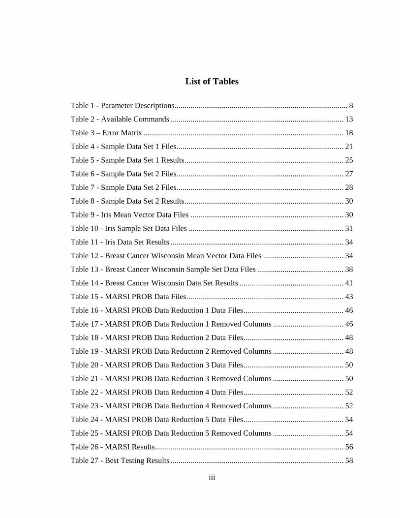
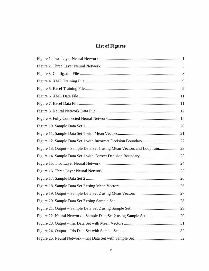
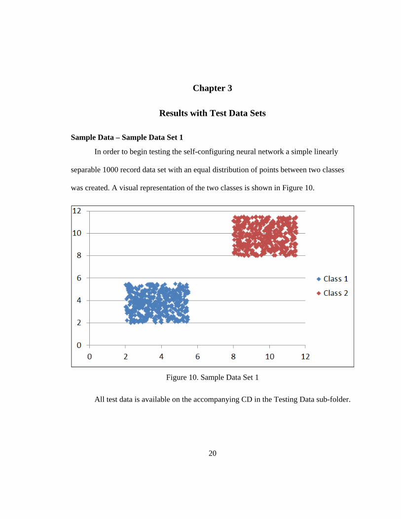
Figure 10. Sample Data Set 1 ........................................................................................... 20 

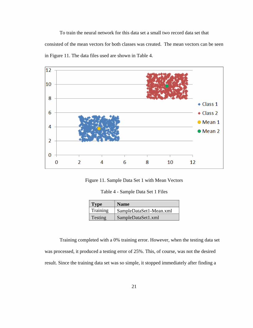
Figure 11. Sample Data Set 1 with Mean Vectors ............................................................ 21 

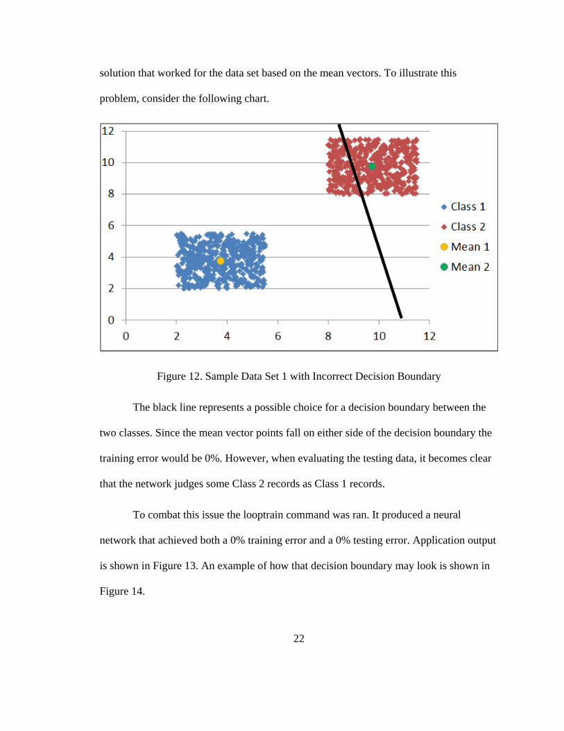
Figure 12. Sample Data Set 1 with Incorrect Decision Boundary .................................... 22 

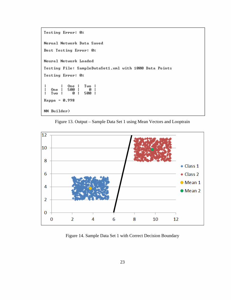
Figure 13. Output – Sample Data Set 1 using Mean Vectors and Looptrain .................... 23 

Figure 14. Sample Data Set 1 with Correct Decision Boundary ...................................... 23 

Figure 15. Two Layer Neural Network ............................................................................. 24 

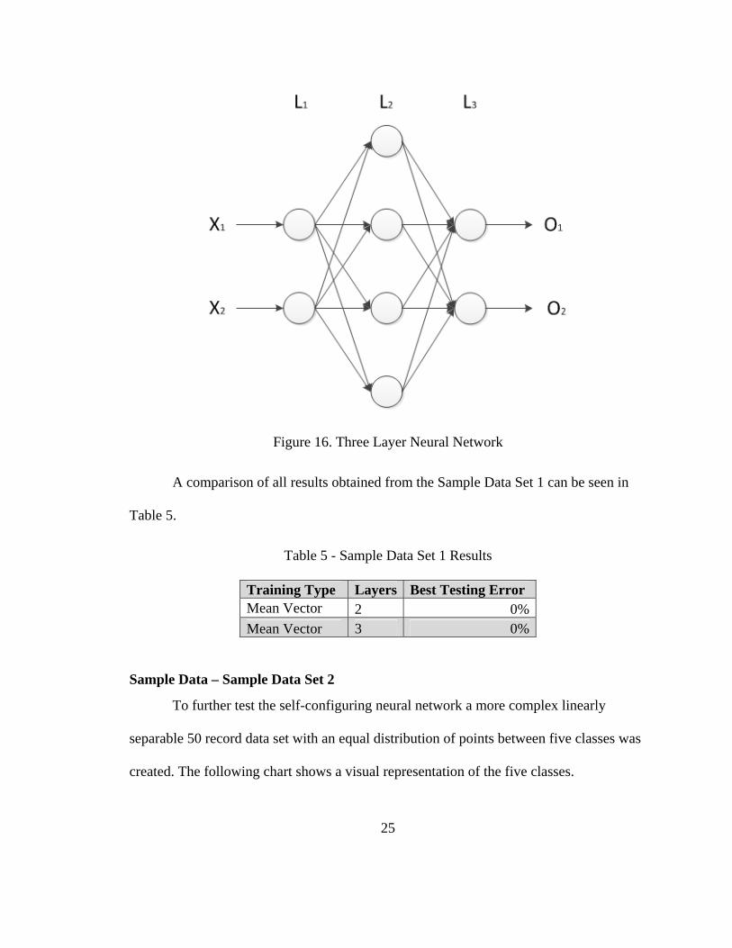
Figure 16. Three Layer Neural Network ........................................................................... 25 

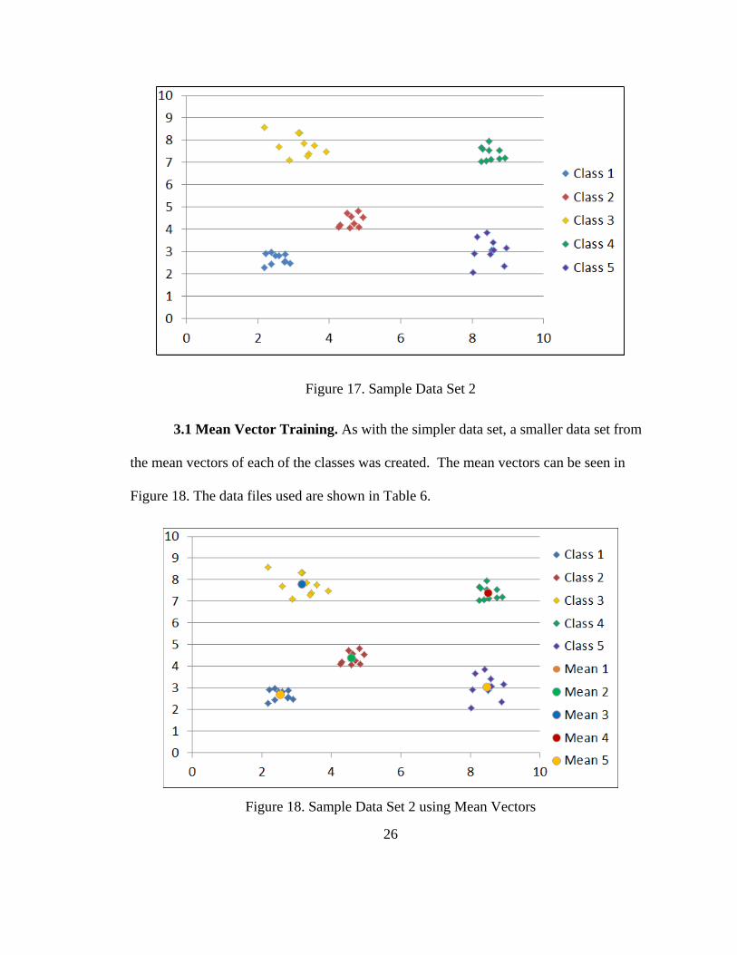
Figure 17. Sample Data Set 2 ........................................................................................... 26 

Figure 18. Sample Data Set 2 using Mean Vectors .......................................................... 26 

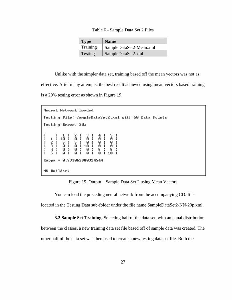
Figure 19. Output – Sample Data Set 2 using Mean Vectors ........................................... 27 

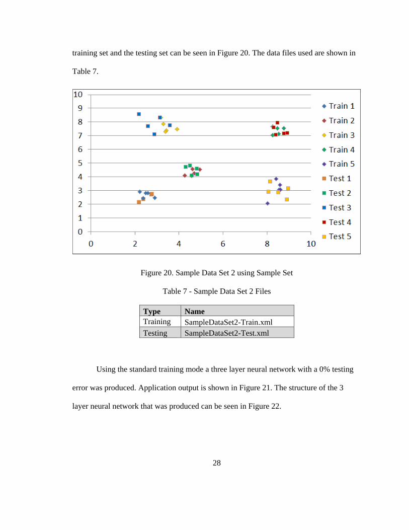
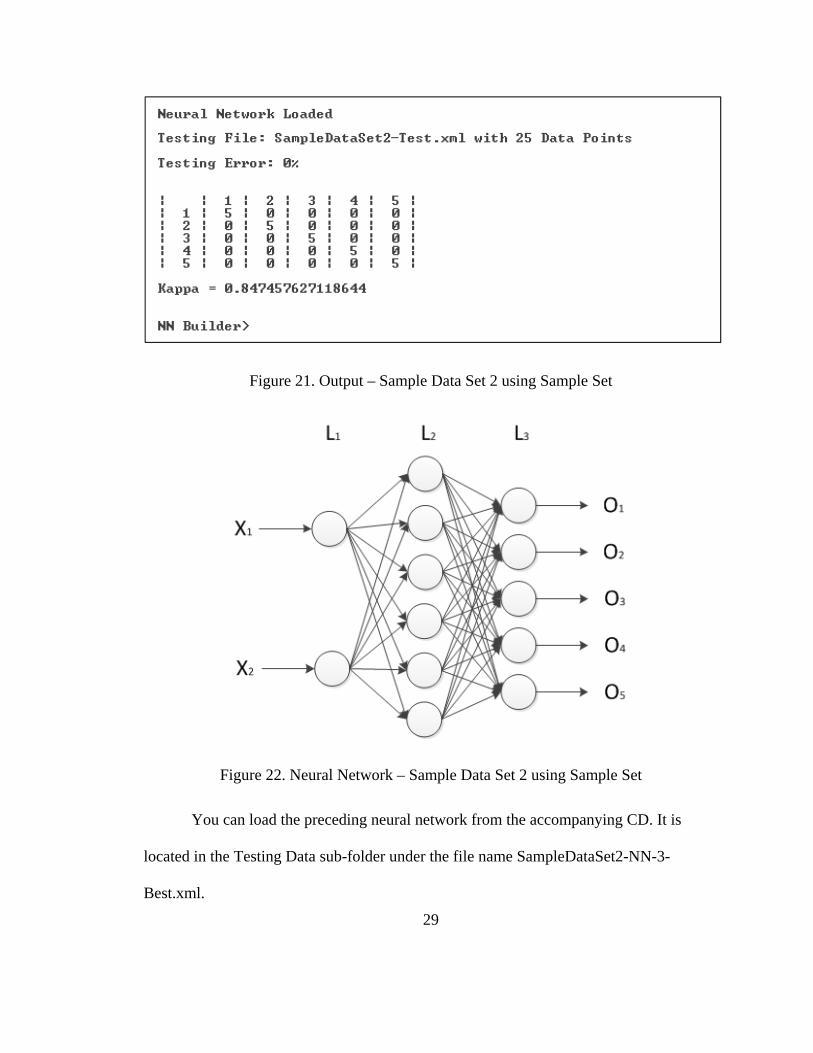
Figure 20. Sample Data Set 2 using Sample Set ............................................................... 28 

Figure 21. Output – Sample Data Set 2 using Sample Set ................................................ 29 

Figure 22. Neural Network – Sample Data Set 2 using Sample Set ................................. 29 

Figure 23. Output – Iris Data Set with Mean Vectors ...................................................... 31 

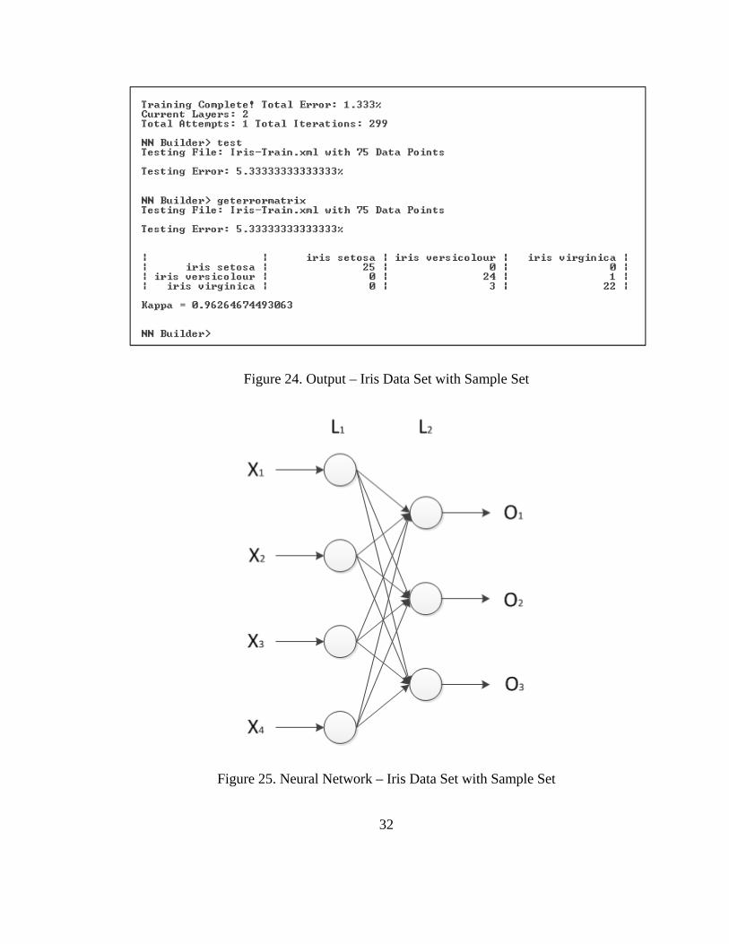
Figure 24. Output – Iris Data Set with Sample Set ........................................................... 32 

Figure 25. Neural Network – Iris Data Set with Sample Set ............................................ 32 

vi

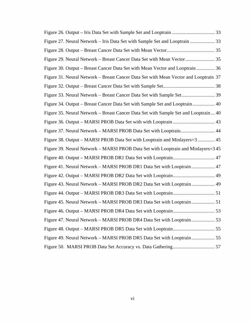
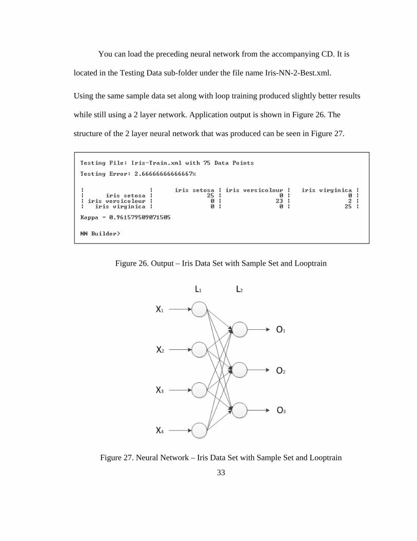
Figure 26. Output – Iris Data Set with Sample Set and Looptrain ................................... 33 

Figure 27. Neural Network – Iris Data Set with Sample Set and Looptrain .................... 33 

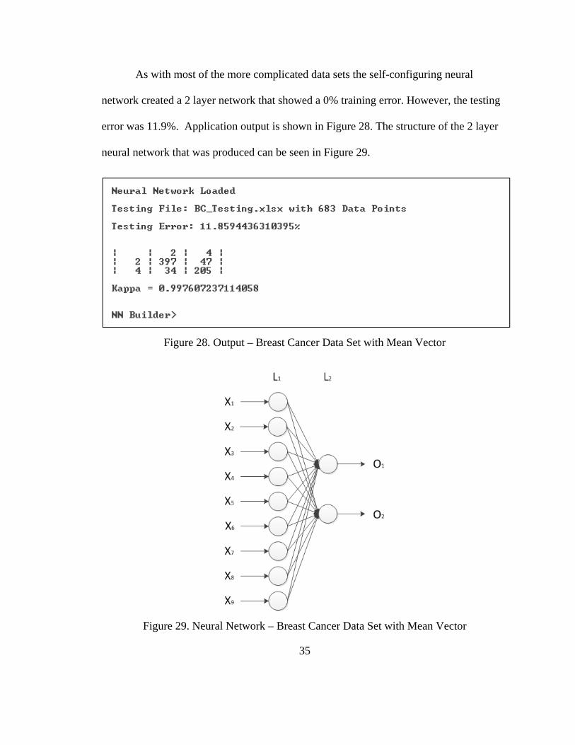
Figure 28. Output – Breast Cancer Data Set with Mean Vector ....................................... 35 

Figure 29. Neural Network – Breast Cancer Data Set with Mean Vector ........................ 35 

Figure 30. Output – Breast Cancer Data Set with Mean Vector and Looptrain ............... 36 

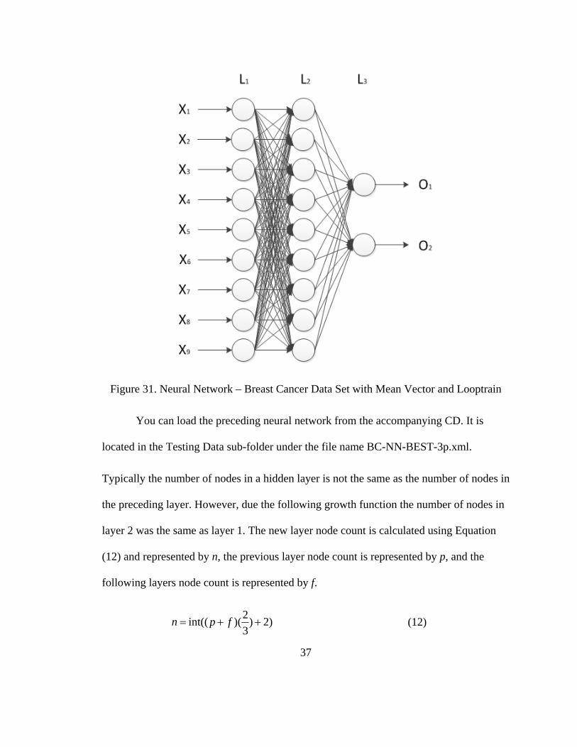
Figure 31. Neural Network – Breast Cancer Data Set with Mean Vector and Looptrain 37 

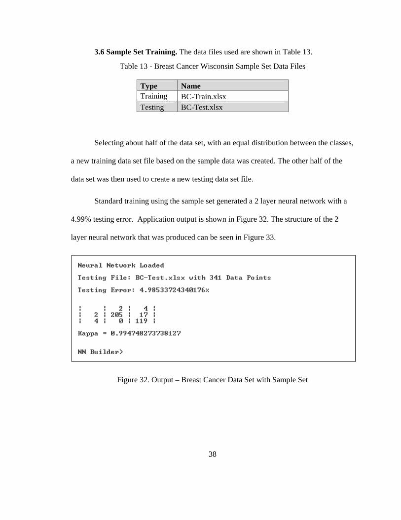
Figure 32. Output – Breast Cancer Data Set with Sample Set .......................................... 38 

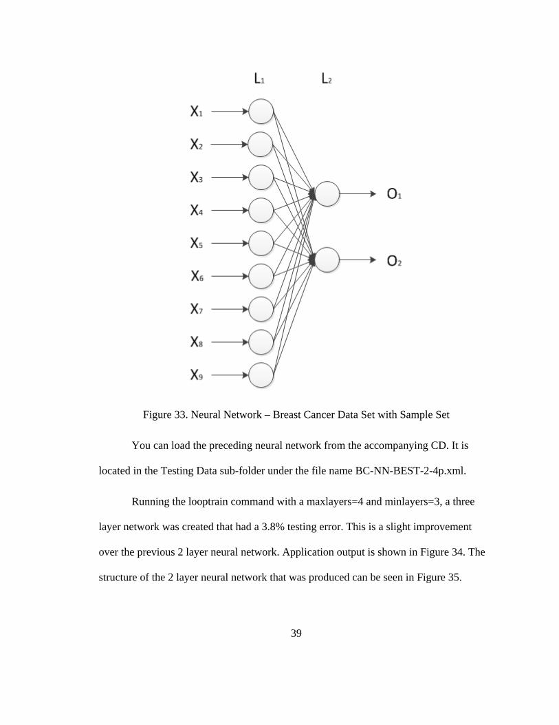
Figure 33. Neural Network – Breast Cancer Data Set with Sample Set ........................... 39 

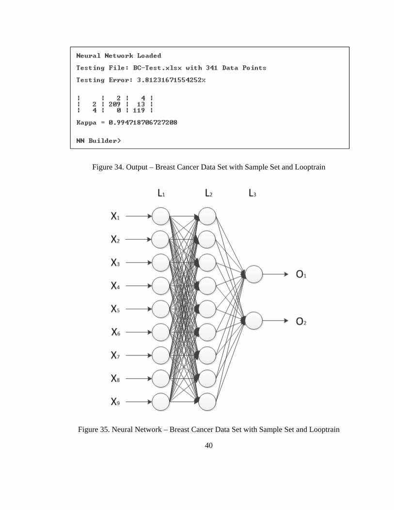
Figure 34. Output – Breast Cancer Data Set with Sample Set and Looptrain .................. 40 

Figure 35. Neural Network – Breast Cancer Data Set with Sample Set and Looptrain ... 40 

Figure 36. Output – MARSI PROB Data Set with with Looptrain .................................. 43 

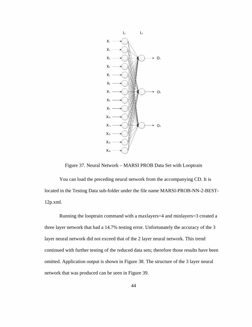
Figure 37. Neural Network – MARSI PROB Data Set with Looptrain ............................ 44 

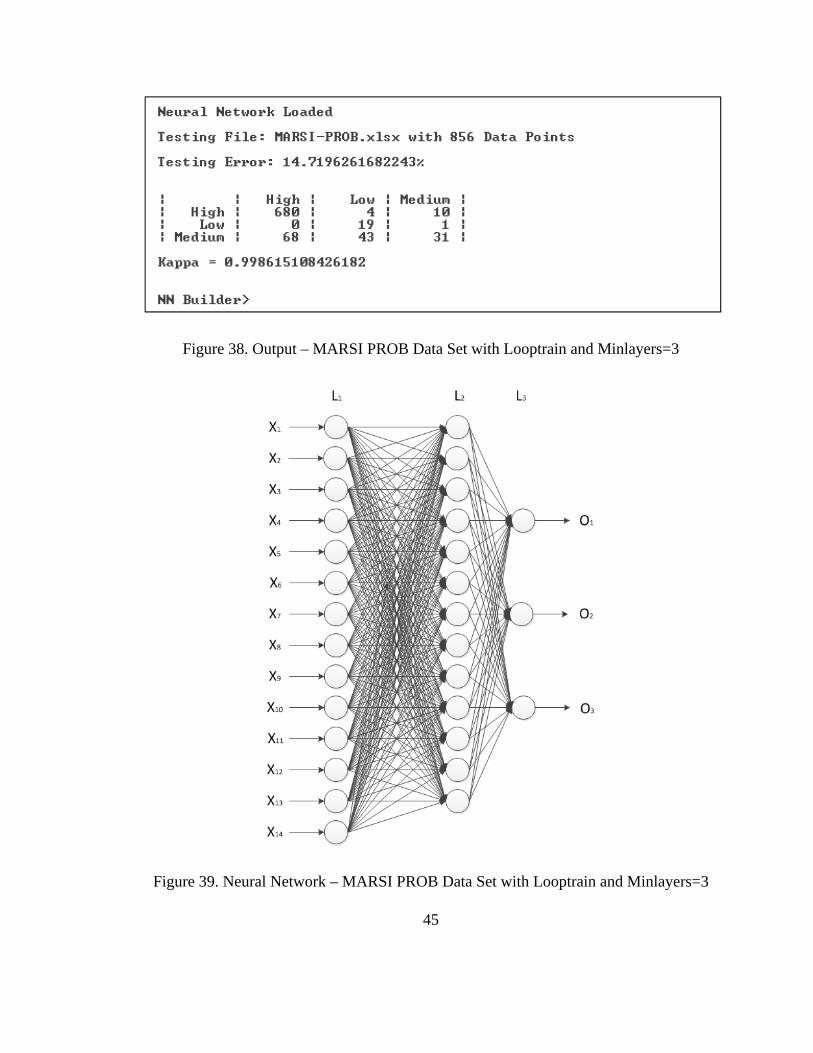
Figure 38. Output – MARSI PROB Data Set with Looptrain and Minlayers=3 .............. 45 

Figure 39. Neural Network – MARSI PROB Data Set with Looptrain and Minlayers=3 45 

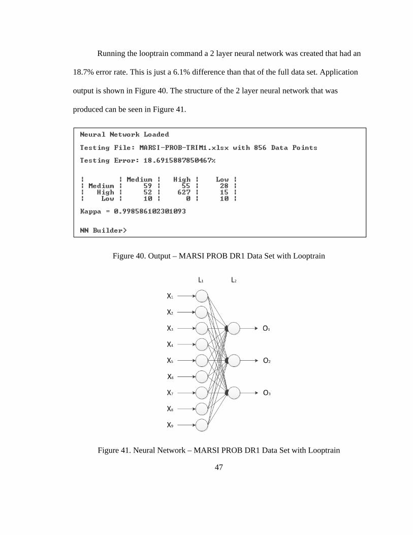
Figure 40. Output – MARSI PROB DR1 Data Set with Looptrain .................................. 47 

Figure 41. Neural Network – MARSI PROB DR1 Data Set with Looptrain ................... 47 

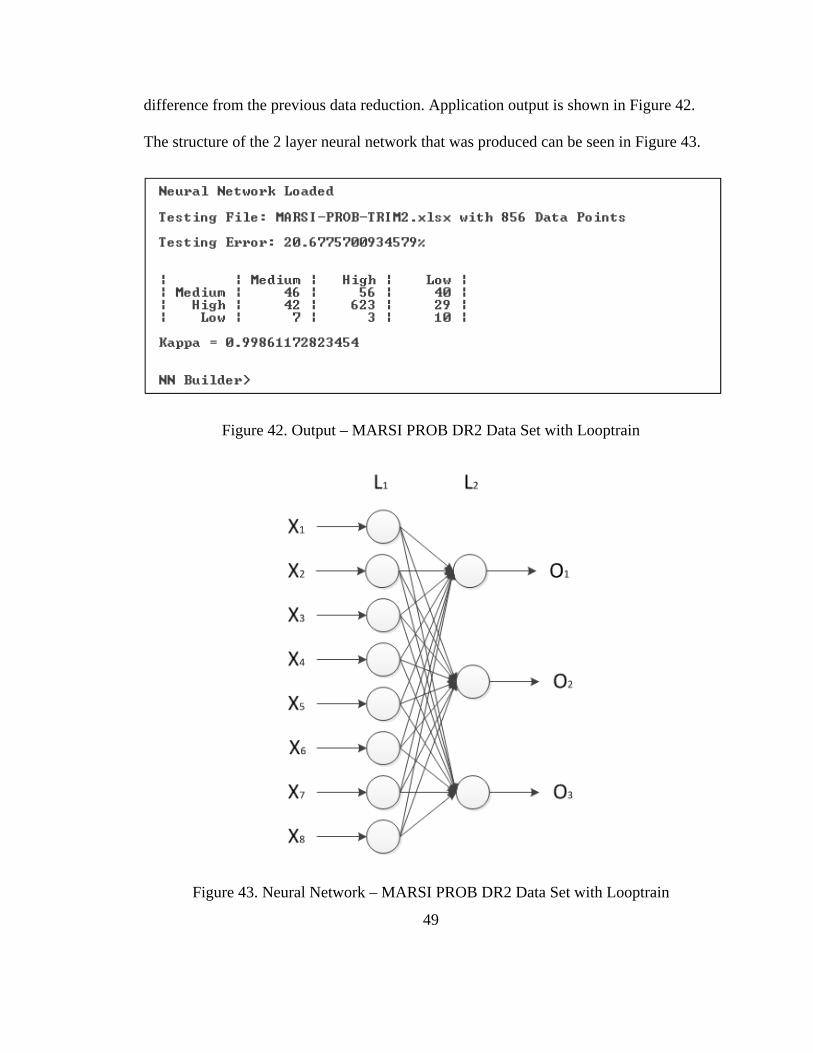
Figure 42. Output – MARSI PROB DR2 Data Set with Looptrain .................................. 49 

Figure 43. Neural Network – MARSI PROB DR2 Data Set with Looptrain ................... 49 

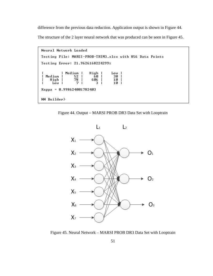
Figure 44. Output – MARSI PROB DR3 Data Set with Looptrain .................................. 51 

Figure 45. Neural Network – MARSI PROB DR3 Data Set with Looptrain ................... 51 

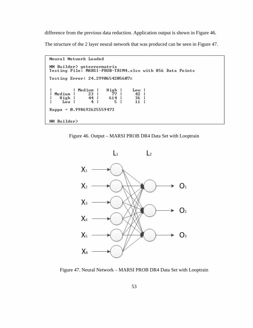
Figure 46. Output – MARSI PROB DR4 Data Set with Looptrain .................................. 53 

Figure 47. Neural Network – MARSI PROB DR4 Data Set with Looptrain ................... 53 

Figure 48. Output – MARSI PROB DR5 Data Set with Looptrain .................................. 55 

Figure 49. Neural Network – MARSI PROB DR5 Data Set with Looptrain ................... 55 

Figure 50. MARSI PROB Data Set Accuracy vs. Data Gathering .................................. 57 

vii

Abstract

SELF-CONFIGURING NEURAL NETWORKS

JUSTIN M. ANDERSON

Thesis Chair: Arun Kulkarni, Ph.D.

The University of Texas at Tyler

December 2012

Neural Networks are an effective means of classifying data; however they are usually

purpose built applications that are created for classifying a single data set. Programming

a neural network can be a time consuming and sometimes error prone process. To

alleviate both of these problems a self-configuring multilayer perceptron model was used

to create and train neural networks. This application can take any training data set that is

linearly or nonlinearly separable as input, then create the needed neural network structure

and train itself, thus saving programmers’ time and effort. The software has been tested

with several data sets including sample data sets, the Iris data set, and the MARSI data

set. The results indicate that once the network is created and trained, it can be used to

effectively classify data from many data sets.

1

Chapter 1

Introduction

Neural networks are primarily purpose built applications that are used to classify

data from a specific data set. Programming a neural network can be a time consuming

and sometimes error prone process. A self-configuring neural network can take any data

set that is separable as input and create the needed neural network configuration, thus

saving programmers’ time and effort. The only requirements are that the data set must be

separable and supports supervised learning.

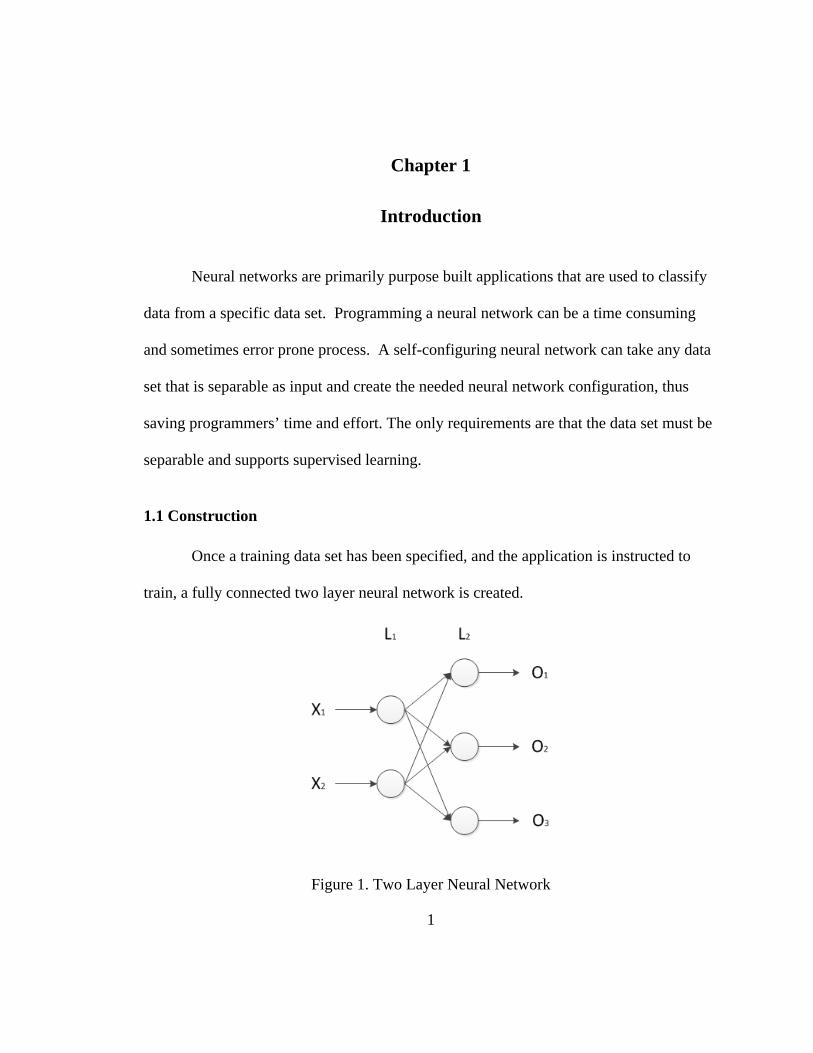
1.1 Construction

Once a training data set has been specified, and the application is instructed to

train, a fully connected two layer neural network is created.

Figure 1. Two Layer Neural Network

2

In L1 an artificial neuron (McCulloch & Pitts, 1943), or node, for each input in

the data set is created with the addition of a small randomized weight on each input.

Weights on the inputs help the neural network more easily adapt to data sets that contain

non-normalized values.

The second layer contains a node for each output class. Each output node is fully

connected to every input node using a small random weight. Once data is feed into the

network and has propagated to the output nodes, then the node with the highest value is

considered the winner.

1.2 Learning Algorithm

The back-propagation learning algorithm (Rumelhart, Hinton, & Williams, 1986)

is described below (Kulkarni, 2001).

Step 1: Initialize the weights. The weights between layers L1L2 and L2L3 are represented

by elements of matrices P and Q. These weights are initialized to small random values so

that the network is not saturated by large values of weights. Let n and m represent the

number of units in layers L1, and L2, respectively. Let l represent units in L3. In this case l

is equal to 1.

S

th

ca

In

re

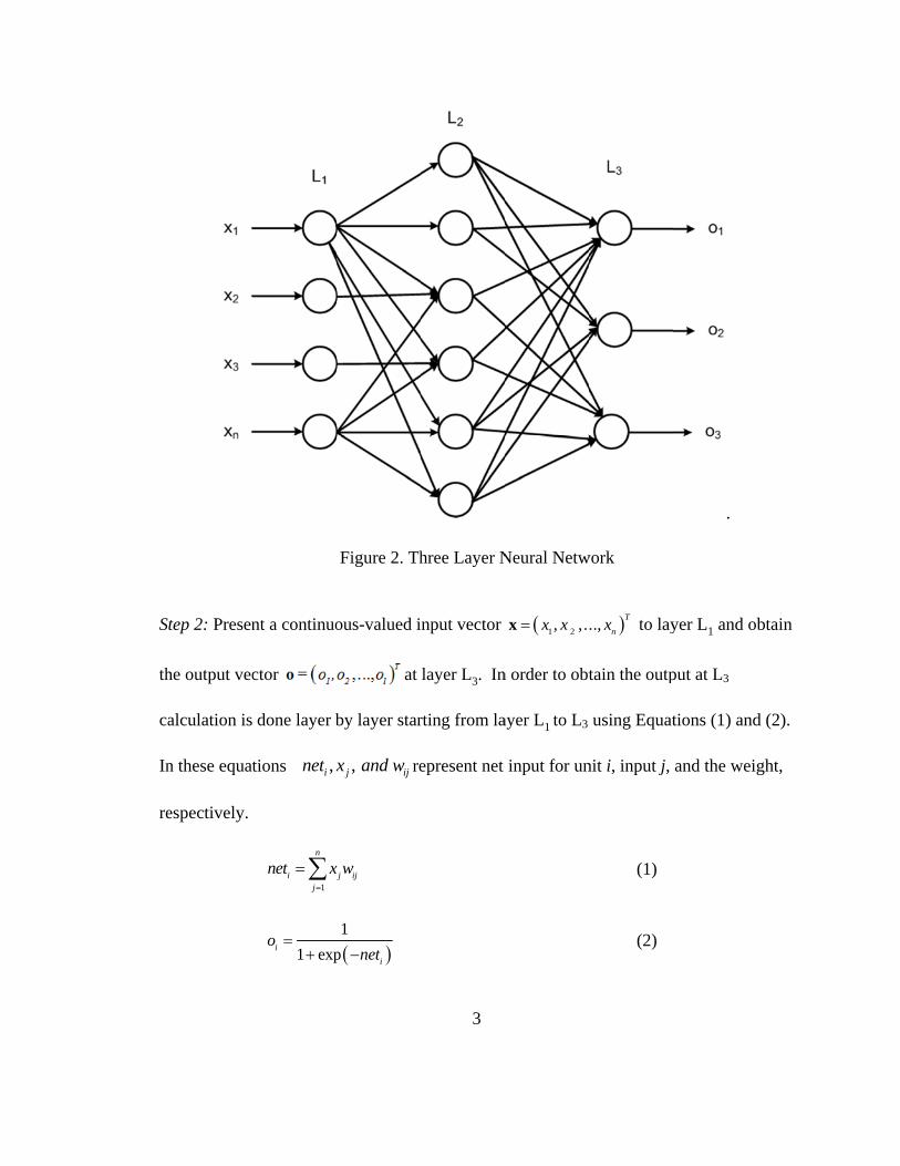
Step 2: Presen

he output vec

alculation is

n these equat

espectively.

nt a continuo

ctor

done layer b

tions ,inet x

1

n

i jj

net x=

=∑

1 expio =+

Figure 2. Th

ous-valued i

at

by layer star

,j ijx and w re

j ijx w

( )1

p inet−

3

hree Layer N

nput vector

layer L3. In

rting from la

epresent net

Neural Netw

( 1 2, ,..x x=x

n order to obt

ayer L1 to L3

input for un

work

).., T

nx to lay

tain the outp

using Equat

nit i, input j,

(1)

(2)

.

yer L1 and ob

put at L3

tions (1) and

and the weig

btain

d (2).

ght,

4

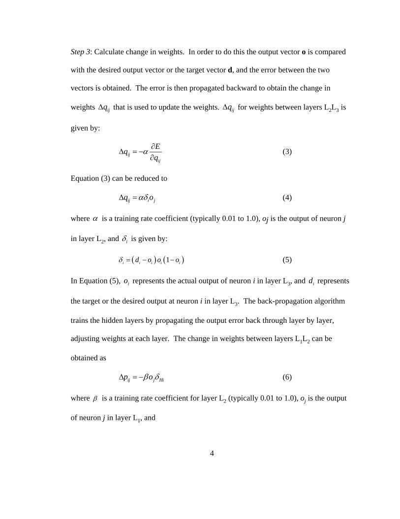
Step 3: Calculate change in weights. In order to do this the output vector o is compared

with the desired output vector or the target vector d, and the error between the two

vectors is obtained. The error is then propagated backward to obtain the change in

weights ijqΔ that is used to update the weights. ijqΔ for weights between layers L2L3 is

given by:

ijij

Eqq

α ∂Δ = −

∂ (3)

Equation (3) can be reduced to

ij i jq oαδΔ = (4)

where α is a training rate coefficient (typically 0.01 to 1.0), oj is the output of neuron j

in layer L2, and iδ is given by:

( ) ( )1i i i i id o o oδ = − − (5)

In Equation (5), io represents the actual output of neuron i in layer L3, and id represents

the target or the desired output at neuron i in layer L3. The back-propagation algorithm

trains the hidden layers by propagating the output error back through layer by layer,

adjusting weights at each layer. The change in weights between layers L1L2 can be

obtained as

ij j Hip oβ δΔ = − (6)

where β is a training rate coefficient for layer L2 (typically 0.01 to 1.0), oj is the output

of neuron j in layer L1, and

5

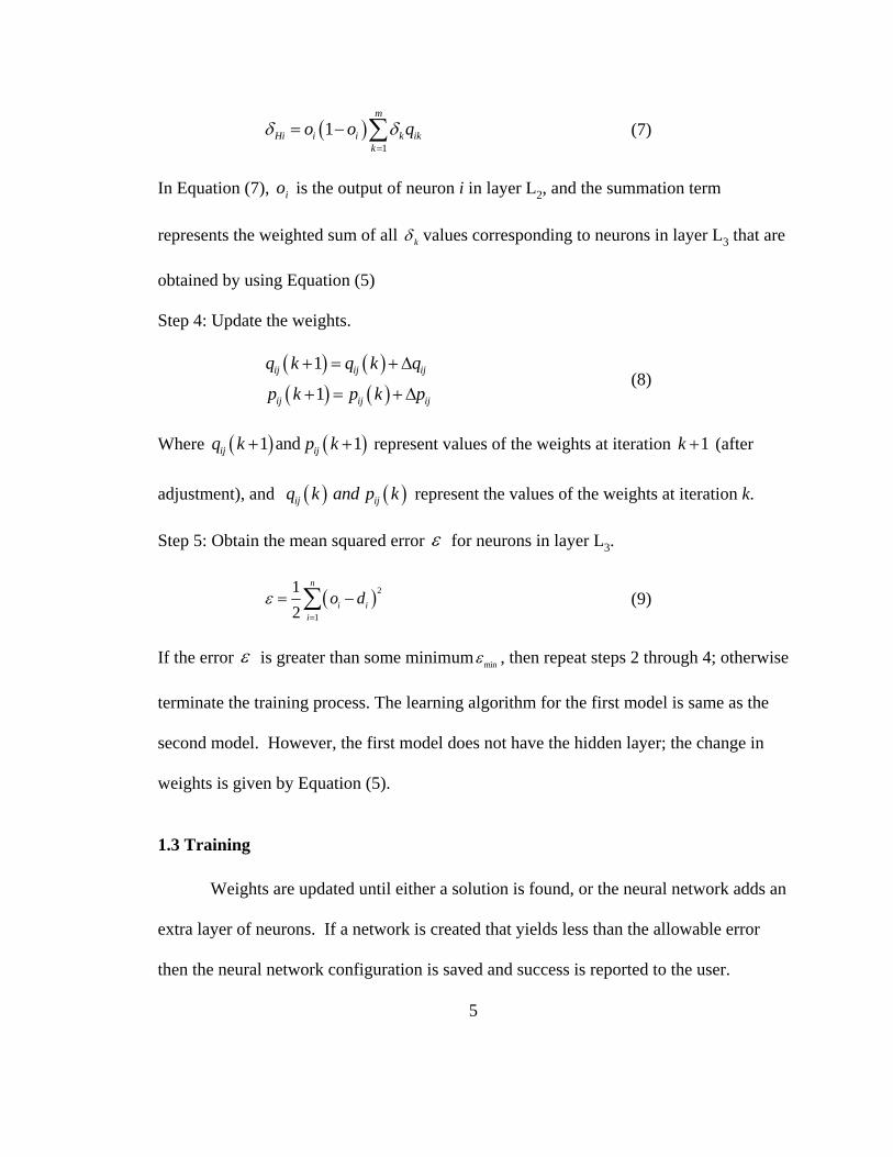
( )1

1m

Hi i i k ikk

o o qδ δ=

= − ∑ (7)

In Equation (7), io is the output of neuron i in layer L2, and the summation term

represents the weighted sum of all kδ values corresponding to neurons in layer L3 that are

obtained by using Equation (5)

Step 4: Update the weights.

( ) ( )( ) ( )

1

1ij ij ij

ij ij ij

q k q k q

p k p k p

+ = +Δ

+ = +Δ (8)

Where ( ) ( )1 and 1ij ijq k p k+ + represent values of the weights at iteration 1k + (after

adjustment), and ( ) ( )ij ijq k and p k represent the values of the weights at iteration k.

Step 5: Obtain the mean squared error ε for neurons in layer L3.

( )2

1

12

n

i ii

o dε=

= −∑ (9)

If the error ε is greater than some minimum minε , then repeat steps 2 through 4; otherwise

terminate the training process. The learning algorithm for the first model is same as the

second model. However, the first model does not have the hidden layer; the change in

weights is given by Equation (5).

1.3 Training

Weights are updated until either a solution is found, or the neural network adds an

extra layer of neurons. If a network is created that yields less than the allowable error

then the neural network configuration is saved and success is reported to the user.

6

1.4 Growth

If the training algorithm processes through the entire training set for the specified

iterations and did not find a neural network that produces less than the configured

allowable error, then an extra layer of neurons is added, and all the weights are

randomized. At this point the system would run through the training process again until

either a solution is found, or the neural network adds an extra layer or neurons.

1.5 Live Data

Once a neural network has been created and trained it can be used to process live

data. Once the data is processed it is saved to a separate file.

7

Chapter 2

Methodology

Program Specification

In order to use the Self-Configuring Neural Network, several files must be

prepared first.

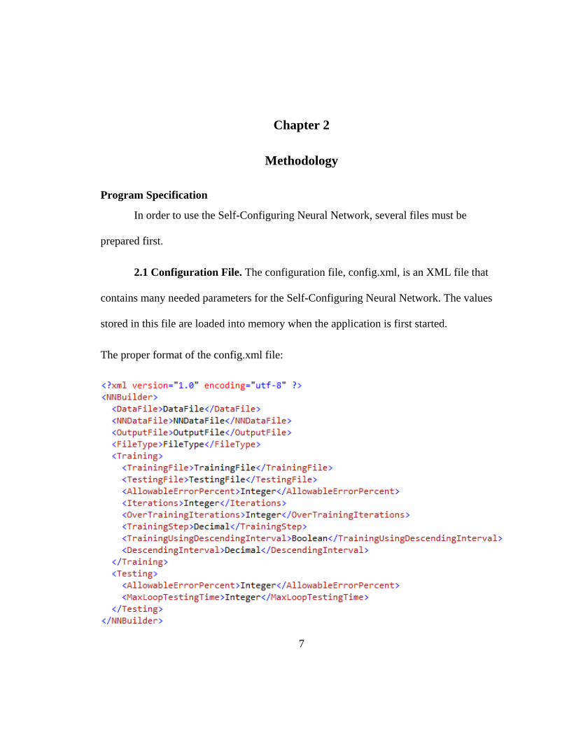
2.1 Configuration File. The configuration file, config.xml, is an XML file that

contains many needed parameters for the Self-Configuring Neural Network. The values

stored in this file are loaded into memory when the application is first started.

The proper format of the config.xml file:

8

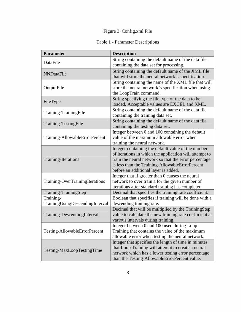
Figure 3. Config.xml File

Table 1 - Parameter Descriptions

Parameter Description

DataFile String containing the default name of the data file containing the data set for processing.

NNDataFile String containing the default name of the XML file that will store the neural network’s specification.

OutputFile String containing the name of the XML file that will store the neural network’s specification when using the LoopTrain command.

FileType String specifying the file type of the data to be loaded. Acceptable values are EXCEL and XML.

Training-TrainingFile String containing the default name of the data file containing the training data set.

Training-TestingFile String containing the default name of the data file containing the testing data set.

Training-AllowableErrorPercent Integer between 0 and 100 containing the default value of the maximum allowable error when training the neural network.

Training-Iterations

Integer containing the default value of the number of iterations in which the application will attempt to train the neural network so that the error percentage is less than the Training-AllowableErrorPercent before an additional layer is added.

Training-OverTrainingIterations Integer that if greater than 0 causes the neural network to over train a for the given number of iterations after standard training has completed.

Training-TrainingStep Decimal that specifies the training rate coefficient. Training-TrainingUsingDescendingInterval

Boolean that specifies if training will be done with a descending training rate.

Training-DescendingInterval Decimal that will be multiplied by the TrainingStep value to calculate the new training rate coefficient at various intervals during training.

Testing-AllowableErrorPercent Integer between 0 and 100 used during Loop Training that contains the value of the maximum allowable error when testing the neural network.

Testing-MaxLoopTestingTime

Integer that specifies the length of time in minutes that Loop Training will attempt to create a neural network which has a lower testing error percentage than the Testing-AllowableErrorPercent value.

9

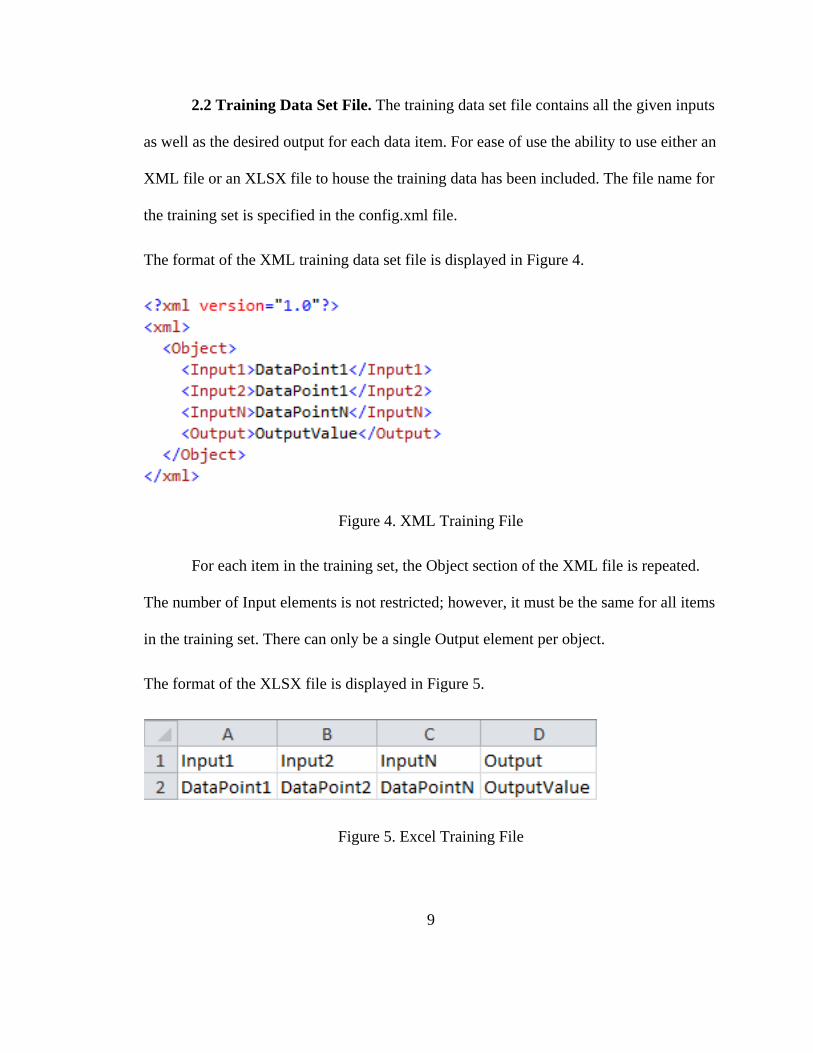
2.2 Training Data Set File. The training data set file contains all the given inputs

as well as the desired output for each data item. For ease of use the ability to use either an

XML file or an XLSX file to house the training data has been included. The file name for

the training set is specified in the config.xml file.

The format of the XML training data set file is displayed in Figure 4.

Figure 4. XML Training File

For each item in the training set, the Object section of the XML file is repeated.

The number of Input elements is not restricted; however, it must be the same for all items

in the training set. There can only be a single Output element per object.

The format of the XLSX file is displayed in Figure 5.

Figure 5. Excel Training File

10

The first row contains the input variable names and also specifies the Output

value. For each item in the training set, a new row is added below the first row. Similar to

its XML counterpart the number of Input elements is not restricted; however, it must be

the same for all items in the training set. There can only be a single Output element per

item.

2.3 Testing Data Set File. The testing data set file has the same structure as the

train data set file. It contains all the given inputs as well as the desired output for each

data item. For ease of use the ability to use either an XML file or an XLSX file to house

the testing data has been included. The file name for the testing data set file is specified in

the config.xml file.

2.4 Data File. The data file contains the data that needs to be classified. It very

similar to both the training and testing data set files with the exception of not including

the output values. The data file contains all the given inputs for each data item. For ease

of use the ability to use either an XML file or an XLSX file to house the data has been

included. The file name for the data file is specified in the config.xml file.

The proper format of the XML file is displayed in Figure 6.

11

Figure 6. XML Data File

For each item in the data set, the Object section of the XML file is repeated. The

number of Input elements is not restricted; however, it must be the same for all items in

the training set.

The proper format of the XLSX file is displayed in Figure 7.

Figure 7. Excel Data File

The first row contains the Input Variable names. For each item in the training set,

a new row is added below the first row. Similar to its XML counterpart, the number of

Input elements is not restricted; however, it must be the same for all items in the training

set.

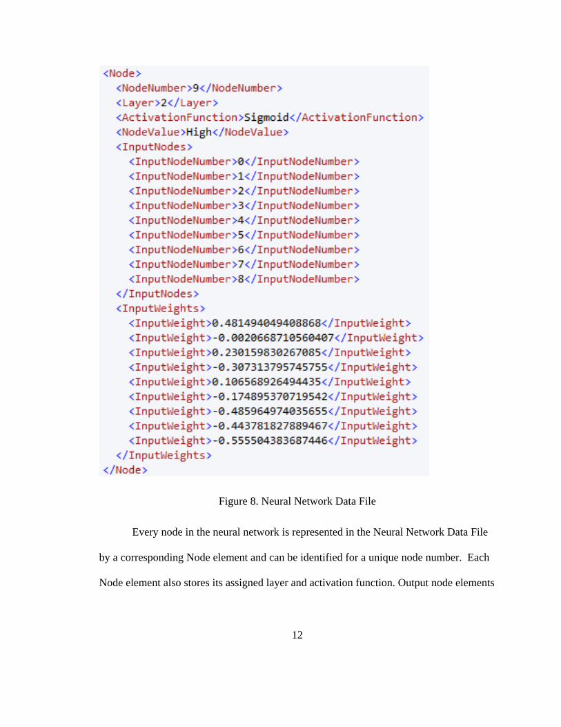
2.5 Neural Network Data File. The Neural Network Data File, or NNDataFile, is

an XML representation for the neural network created during training. This allows us to

create and train a self-configuring neural network and then save its structure for later use.

An excerpt from a Neural Network Data File is displayed in Figure 8.

12

Figure 8. Neural Network Data File

Every node in the neural network is represented in the Neural Network Data File

by a corresponding Node element and can be identified for a unique node number. Each

Node element also stores its assigned layer and activation function. Output node elements

13

also contain the value of their class. A list of input nodes and their input weights is

stored. From this data a complete neural network can be created.

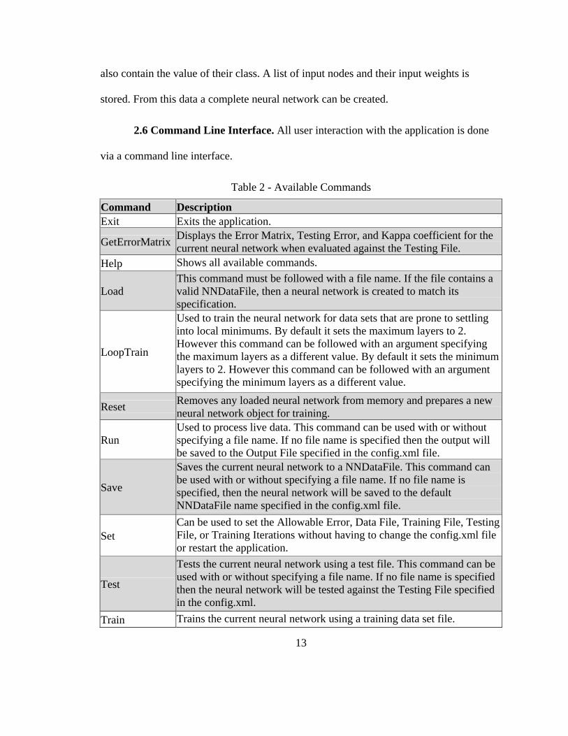
2.6 Command Line Interface. All user interaction with the application is done

via a command line interface.

Table 2 - Available Commands

Command Description Exit Exits the application.

GetErrorMatrix Displays the Error Matrix, Testing Error, and Kappa coefficient for the current neural network when evaluated against the Testing File.

Help Shows all available commands.

Load This command must be followed with a file name. If the file contains a valid NNDataFile, then a neural network is created to match its specification.

LoopTrain

Used to train the neural network for data sets that are prone to settling into local minimums. By default it sets the maximum layers to 2. However this command can be followed with an argument specifying the maximum layers as a different value. By default it sets the minimum layers to 2. However this command can be followed with an argument specifying the minimum layers as a different value.

Reset Removes any loaded neural network from memory and prepares a new neural network object for training.

Run Used to process live data. This command can be used with or without specifying a file name. If no file name is specified then the output will be saved to the Output File specified in the config.xml file.

Save

Saves the current neural network to a NNDataFile. This command can be used with or without specifying a file name. If no file name is specified, then the neural network will be saved to the default NNDataFile name specified in the config.xml file.

Set Can be used to set the Allowable Error, Data File, Training File, Testing File, or Training Iterations without having to change the config.xml file or restart the application.

Test

Tests the current neural network using a test file. This command can be used with or without specifying a file name. If no file name is specified then the neural network will be tested against the Testing File specified in the config.xml.

Train Trains the current neural network using a training data set file.

14

Program Operation

This self-configuring neural network uses a very specialized training function.

While most neural networks’ training functions just alter the weights on the inputs to

nodes in their networks, this training function also has the ability to grow the network by

adding additional neurons and layers.

2.7 Preprocessing. Before the training phase begins training data must be

available in an acceptable format, which is either XML or Excel as specified earlier.

Using the test data to generate mean vectors was the preferred method of training due to

the reduced training set, which in turn speeds up neural network creation. Thus the mean

vectors become the Training File and the original training data becomes the Testing File.

2.8 Training. In order to create a neural network for a new data set, the training

data set’s file name needs to first be entered into the config.xml file, and the file should

be placed in the same folder as the application. Next run the SCNN.exe application, and

type in the command “train”.

The first step of the training is to load all data from the training data set file into a

.NET DataTable. Next the number of inputs and the number and type of outputs classes is

derived from the provided training data. This information is then used to instantiate a new

fully connected back-propagation (Kulkarni, 2001) neural network with randomized input

weights as shown in Figure 9.

15

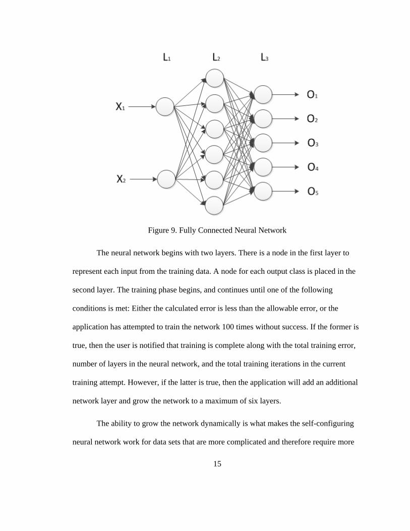
Figure 9. Fully Connected Neural Network

The neural network begins with two layers. There is a node in the first layer to

represent each input from the training data. A node for each output class is placed in the

second layer. The training phase begins, and continues until one of the following

conditions is met: Either the calculated error is less than the allowable error, or the

application has attempted to train the network 100 times without success. If the former is

true, then the user is notified that training is complete along with the total training error,

number of layers in the neural network, and the total training iterations in the current

training attempt. However, if the latter is true, then the application will add an additional

network layer and grow the network to a maximum of six layers.

The ability to grow the network dynamically is what makes the self-configuring

neural network work for data sets that are more complicated and therefore require more

16

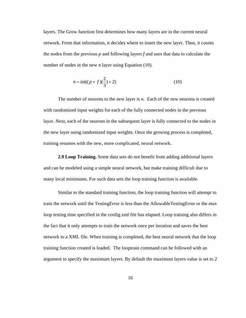
layers. The Grow function first determines how many layers are in the current neural

network. From that information, it decides where to insert the new layer. Then, it counts

the nodes from the previous p and following layers f and uses that data to calculate the

number of nodes in the new n layer using Equation (10).

)2)32)(int(( ++= fpn (10)

The number of neurons to the new layer is n. Each of the new neurons is created

with randomized input weights for each of the fully connected nodes in the previous

layer. Next, each of the neurons in the subsequent layer is fully connected to the nodes in

the new layer using randomized input weights. Once the growing process is completed,

training resumes with the new, more complicated, neural network.

2.9 Loop Training. Some data sets do not benefit from adding additional layers

and can be modeled using a simple neural network, but make training difficult due to

many local minimums. For such data sets the loop training function is available.

Similar to the standard training function, the loop training function will attempt to

train the network until the TestingError is less than the AllowableTestingError or the max

loop testing time specified in the config.xml file has elapsed. Loop training also differs in

the fact that it only attempts to train the network once per iteration and saves the best

network to a XML file. When training is completed, the best neural network that the loop

training function created is loaded. The looptrain command can be followed with an

argument to specify the maximum layers. By default the maximum layers value is set to 2

17

for loop training. The looptrain command can also be followed with an argument to

specify the minimum layers. By default the minimum layers value is set to 2 for loop

training. Setting the minimum layers is useful when training with mean vectors on more

complex data sets. When set to a value greater than 2, it keeps the generated neural

network from being overly simplistic.

2.10 Over Training. Over Training, when enabled via the config.xml file, allows

the neural network to be trained using a smaller training step after the original allowable

error percentage is achieved. When enabled, on some data sets, the testing error is

reduced by a noticeable amount. Once over training mode is entered, the training step, or

alpha, is reduced to a tenth or its original value. Also the upper training limit is changed

from 0.7 to 0.9. Likewise the lower training limit is changed from 0.3 to 0.1. This fine

tuning of the neural networks can help to achieve a more accurate model.

2.11 Testing. The Test function loads the test data set from the file specified in

the config.xml file into a .NET DataSet object. Next it runs the data set though the loaded

neural network and compares the output value specified in the testing data set file to that

of the neural network. Once all records from the testing data set file are processed, the

data is then used to calculate an overall testing error, which is then displayed in the

interface.

A more advanced test function can be accessed by running the geterrormatrix

command. This function is the same as the regular test function but also includes an error

matrix and the kappa coefficient.

18

An error matrix, also called a confusion matrix (Kohavi & Provost, 1998), is a

square matrix that shows the performance of a classification algorithm in a table. Each

column of the matrix represents the instances in a predicted class, while each row

represents the instances in an actual class. Table 3 shows an example error matrix for a

100 item set consisting of two classes.

Table 3 – Error Matrix

actual \ predicted Negative Positive Negative 47 3 Positive 14 36

The kappa coefficient is a statistical measure of inter-rater agreement or inter-

annotator agreement (Bishop, Fienberg, & Holland, 1975) for categorical items. It is

calculated using Equation (11).

where K is the kappa coefficient, r is the number of rows, xii is the number of

observations in row I and column I, xi+ is the total of row I, x+i is the total of column I,

and N is the total number of observations.

2.12 Live Data. The Run command is used to process live data though the neural

network. It can be used with or without specifying a file name. If no file name is

specified then the output will be saved to the Output File specified in the config.xml file.

(11)

19

The structure of the output file should be the same as the input file with the addition of an

output column.

20

Chapter 3

Results with Test Data Sets

Sample Data – Sample Data Set 1

In order to begin testing the self-configuring neural network a simple linearly

separable 1000 record data set with an equal distribution of points between two classes

was created. A visual representation of the two classes is shown in Figure 10.

Figure 10. Sample Data Set 1

All test data is available on the accompanying CD in the Testing Data sub-folder.

21

To train the neural network for this data set a small two record data set that

consisted of the mean vectors for both classes was created. The mean vectors can be seen

in Figure 11. The data files used are shown in Table 4.

Figure 11. Sample Data Set 1 with Mean Vectors

Table 4 - Sample Data Set 1 Files

Type Name Training SampleDataSet1-Mean.xml Testing SampleDataSet1.xml

Training completed with a 0% training error. However, when the testing data set

was processed, it produced a testing error of 25%. This, of course, was not the desired

result. Since the training data set was so simple, it stopped immediately after finding a

22

solution that worked for the data set based on the mean vectors. To illustrate this

problem, consider the following chart.

Figure 12. Sample Data Set 1 with Incorrect Decision Boundary

The black line represents a possible choice for a decision boundary between the

two classes. Since the mean vector points fall on either side of the decision boundary the

training error would be 0%. However, when evaluating the testing data, it becomes clear

that the network judges some Class 2 records as Class 1 records.

To combat this issue the looptrain command was ran. It produced a neural

network that achieved both a 0% training error and a 0% testing error. Application output

is shown in Figure 13. An example of how that decision boundary may look is shown in

Figure 14.

23

Figure 13. Output – Sample Data Set 1 using Mean Vectors and Looptrain

Figure 14. Sample Data Set 1 with Correct Decision Boundary

24

In the example shown in Figure 14 both the mean vector points and their

associated data sets fall on either side of the decision boundary. Therefore both the

training error and testing error is 0%.

Both 2 layer and 3 layer neural networks were generated as solutions to this data

set over the course of testing. The structure of the 2 layer neural network that was

produced can be seen in Figure 15. The 3 layer neural network is shown in Figure 16.

Figure 15. Two Layer Neural Network

You can load the these neural networks from the accompanying CD. They are

located in the Testing Data sub-folder under the file names SampleDataSet1-NN-2-

Best.xml and SampleDataSet1-NN-3-Best.xml, respectively.

25

Figure 16. Three Layer Neural Network

A comparison of all results obtained from the Sample Data Set 1 can be seen in

Table 5.

Table 5 - Sample Data Set 1 Results

Training Type Layers Best Testing Error Mean Vector 2 0% Mean Vector 3 0%

Sample Data – Sample Data Set 2

To further test the self-configuring neural network a more complex linearly

separable 50 record data set with an equal distribution of points between five classes was

created. The following chart shows a visual representation of the five classes.

26

Figure 17. Sample Data Set 2

3.1 Mean Vector Training. As with the simpler data set, a smaller data set from

the mean vectors of each of the classes was created. The mean vectors can be seen in

Figure 18. The data files used are shown in Table 6.

Figure 18. Sample Data Set 2 using Mean Vectors

27

Table 6 - Sample Data Set 2 Files

Type Name Training SampleDataSet2-Mean.xml Testing SampleDataSet2.xml

Unlike with the simpler data set, training based off the mean vectors was not as

effective. After many attempts, the best result achieved using mean vectors based training

is a 20% testing error as shown in Figure 19.

Figure 19. Output – Sample Data Set 2 using Mean Vectors

You can load the preceding neural network from the accompanying CD. It is

located in the Testing Data sub-folder under the file name SampleDataSet2-NN-20p.xml.

3.2 Sample Set Training. Selecting half of the data set, with an equal distribution

between the classes, a new training data set file based off of sample data was created. The

other half of the data set was then used to create a new testing data set file. Both the

28

training set and the testing set can be seen in Figure 20. The data files used are shown in

Table 7.

Figure 20. Sample Data Set 2 using Sample Set

Table 7 - Sample Data Set 2 Files

Type Name Training SampleDataSet2-Train.xml Testing SampleDataSet2-Test.xml

Using the standard training mode a three layer neural network with a 0% testing

error was produced. Application output is shown in Figure 21. The structure of the 3

layer neural network that was produced can be seen in Figure 22.

29

Figure 21. Output – Sample Data Set 2 using Sample Set

Figure 22. Neural Network – Sample Data Set 2 using Sample Set

You can load the preceding neural network from the accompanying CD. It is

located in the Testing Data sub-folder under the file name SampleDataSet2-NN-3-

Best.xml.

30

A comparison of all results obtained from the linearly separable with multiple

classes data set can be seen in Table 8.

Table 8 - Sample Data Set 2 Results

Training Type Layers Best Testing Error Mean Vector 2 20% Sample Set 3 0%

Iris Data Set

To further refine the neural network’s growing and learning algorithms, a copy of

the Iris Data Set (Fisher, 1988) was procured. A reference to this data set can be found in

a great deal of pattern recognition literature. The data set contains 3 classes of 50

instances each, where each class refers to a type of iris plant. One class is linearly

separable from the other 2; the latter are not linearly separable from each other (Fisher,

1936).

3.3 Mean Vector Training. The data files used are shown in Table 9.

Table 9 - Iris Mean Vector Data Files

Type Name Training Iris-Mean.xml Testing Iris.xml

Standard training using the mean vectors was completed with a 0% training error.

However, like Sample Data Set 2, using the mean vectors alone produce a large testing

31

error. For this data set, the best testing error achieved using mean vectors was 36.7%.

Application output is shown in Figure 23.

Figure 23. Output – Iris Data Set with Mean Vectors

3.4 Sample Set Training. The data files used are shown in Table 10.

Table 10 - Iris Sample Set Data Files

Type Name Training Iris-Train.xml Testing Iris-Test.xml

Selecting half of the data set, with an equal distribution between the classes, a

new training data set file based on sample data was created. The other half of the data set

was then used to create a new testing data set file.

Using the standard training mode a two layer neural network with a 5.3% testing

error was created. Application output is shown in Figure 24. The structure of the 2 layer

neural network that was produced can be seen in Figure 25.

32

Figure 24. Output – Iris Data Set with Sample Set

Figure 25. Neural Network – Iris Data Set with Sample Set

33

You can load the preceding neural network from the accompanying CD. It is

located in the Testing Data sub-folder under the file name Iris-NN-2-Best.xml.

Using the same sample data set along with loop training produced slightly better results

while still using a 2 layer network. Application output is shown in Figure 26. The

structure of the 2 layer neural network that was produced can be seen in Figure 27.

Figure 26. Output – Iris Data Set with Sample Set and Looptrain

Figure 27. Neural Network – Iris Data Set with Sample Set and Looptrain

34

You can load the preceding neural network from the accompanying CD. It is

located in the Testing Data sub-folder under the file name Iris-NN-2-BEST-2p.xml.

A comparison of all results obtained from the Iris Data Set can be seen in Table 11.

Table 11 - Iris Data Set Results

Training Type Looptrain Enabled Layers Best Testing Error Mean Vector No 2 36.67%Sample Set No 2 5.33%Sample Set Yes 2 2.67%

Breast Cancer Wisconsin (Diagnostic) Data Set

To further refine the Self-Configuring Neural Network’s ability to work with real

world data, it was used to process the Breast Cancer Wisconsin (Diagnostic) Data Set

(Street, 1995). This data set is comprised of features computed from a digitized image of

a Fine Needle Aspirate (FNA) of a breast mass. They describe characteristics of the cell

nuclei present in the image. A diagnosis of each breast mass, either malignant or benign,

was later determined and assigned to the corresponding record. The diagnosis is used at

the output class for training and testing.

3.5 Mean Vector Training. The data files used are shown in Table 12.

Table 12 - Breast Cancer Wisconsin Mean Vector Data Files

Type Name Training BC_Training-Mean.xlsx Testing BC.xlsx

35

As with most of the more complicated data sets the self-configuring neural

network created a 2 layer network that showed a 0% training error. However, the testing

error was 11.9%. Application output is shown in Figure 28. The structure of the 2 layer

neural network that was produced can be seen in Figure 29.

Figure 28. Output – Breast Cancer Data Set with Mean Vector

Figure 29. Neural Network – Breast Cancer Data Set with Mean Vector

36

The previous result was acceptable; therefore a more complicated neural network

was tested to evaluate if it could do better. The problem is that the mean vector data set is

only comprised of 2 records. When the looptrain algorithm evaluated the mean vectors, it

easily found a 2 layer network that could model them and therefore never had to create a

more complicated network. In order to work around this issue the looptrain algorithm was

updated as to allow setting a minimum layers value so that it could skip training less

complicated networks and move on to larger ones.

Running the looptrain command with a maxlayers=4 and minlayers=3, a three

layer network was created that had a 0% training error and a 3.5% testing error. This is a

vast improvement over the previous results. Application output is shown in Figure 30.

The structure of the 3 layer neural network that was produced can be seen in Figure 31.

Figure 30. Output – Breast Cancer Data Set with Mean Vector and Looptrain

37

Figure 31. Neural Network – Breast Cancer Data Set with Mean Vector and Looptrain

You can load the preceding neural network from the accompanying CD. It is

located in the Testing Data sub-folder under the file name BC-NN-BEST-3p.xml.

Typically the number of nodes in a hidden layer is not the same as the number of nodes in

the preceding layer. However, due the following growth function the number of nodes in

layer 2 was the same as layer 1. The new layer node count is calculated using Equation

(12) and represented by n, the previous layer node count is represented by p, and the

following layers node count is represented by f.

)2)32)(int(( ++= fpn (12)

38

3.6 Sample Set Training. The data files used are shown in Table 13.

Table 13 - Breast Cancer Wisconsin Sample Set Data Files

Type Name Training BC-Train.xlsx Testing BC-Test.xlsx

Selecting about half of the data set, with an equal distribution between the classes,

a new training data set file based on the sample data was created. The other half of the

data set was then used to create a new testing data set file.

Standard training using the sample set generated a 2 layer neural network with a

4.99% testing error. Application output is shown in Figure 32. The structure of the 2

layer neural network that was produced can be seen in Figure 33.

Figure 32. Output – Breast Cancer Data Set with Sample Set

39

Figure 33. Neural Network – Breast Cancer Data Set with Sample Set

You can load the preceding neural network from the accompanying CD. It is

located in the Testing Data sub-folder under the file name BC-NN-BEST-2-4p.xml.

Running the looptrain command with a maxlayers=4 and minlayers=3, a three

layer network was created that had a 3.8% testing error. This is a slight improvement

over the previous 2 layer neural network. Application output is shown in Figure 34. The

structure of the 2 layer neural network that was produced can be seen in Figure 35.

40

Figure 34. Output – Breast Cancer Data Set with Sample Set and Looptrain

Figure 35. Neural Network – Breast Cancer Data Set with Sample Set and Looptrain

41

You can load the preceding neural network from the accompanying CD. It is

located in the Testing Data sub-folder under the file name BC-NN-3-BEST-3.8p.xml.

A comparison of all results obtained from the Breast Cancer Wisconsin Data Set can be

seen in Table 14.

Table 14 - Breast Cancer Wisconsin Data Set Results

Training Type Network Layers Best Testing Error Mean Vector 2 11.86% Mean Vector 3 3.51% Sample Set 2 4.99% Sample Set 3 3.81%

42

Chapter 4

MARSI Data Set Analysis

Metacognitive Awareness-of-Reading Strategies Inventory (MARSI) (Mokhtari &

Reichard, 2002) is a 30-item instrument which was completed by 865 middle school

students. After removing records with missing data, 856 are remaining. MARSI is

specifically designed for measuring students’ metacognitive awareness and use of reading

strategies while reading academic or school-assigned materials. The following data was

collected from the participants’ demographics (e.g., age, grade level, gender, ethnicity,

and perceptions of their ability to read), and perceived awareness and use of reading

strategies, which are organized in three categories, namely global, problem-solving, and

support reading strategies (Anderson, Mokhtari, & Kulkarni, 2012). Using the data

gathered, participants are placed into one of three categories based on the average score

of the perceived awareness section. The three categories are High Level of Awareness

(3.5 or higher), Medium Level of Awareness (2.5-3.4), and Low Level of Awareness (2.4

or lower). This can be calculated overall or based on each category.

The data related to demographics and problem-solving skills was the primary

focus. The goal was to reduce the amount of information needed to be gathered in order

to accurately predict the participants’ categories.

43

Please note all the neural networks for the following MARSI data sets were

training using the overtraining option as it usually reduced the testing error by 0.5-2.0%.

4.1 Overall Accuracy

Table 15 - MARSI PROB Data Files

Type Name Training MARSI-PROB-Mean.xlsx Testing MARSI-PROB.xlsx

To get a baseline for the accuracy, all the data related to global and support

reading strategies was removed and the looptrain algorithm was ran on the remaining

data set. This resulted in a 2 layer neural network with a 12.6% testing error. Application

output is shown in Figure 36. The structure of the 2 layer neural network that was

produced can be seen in Figure 37.

Figure 36. Output – MARSI PROB Data Set with with Looptrain

44

Figure 37. Neural Network – MARSI PROB Data Set with Looptrain

You can load the preceding neural network from the accompanying CD. It is

located in the Testing Data sub-folder under the file name MARSI-PROB-NN-2-BEST-

12p.xml.

Running the looptrain command with a maxlayers=4 and minlayers=3 created a

three layer network that had a 14.7% testing error. Unfortunately the accuracy of the 3

layer neural network did not exceed that of the 2 layer neural network. This trend

continued with further testing of the reduced data sets; therefore those results have been

omitted. Application output is shown in Figure 38. The structure of the 3 layer neural

network that was produced can be seen in Figure 39.

45

Figure 38. Output – MARSI PROB Data Set with Looptrain and Minlayers=3

Figure 39. Neural Network – MARSI PROB Data Set with Looptrain and Minlayers=3

46

You can load the preceding neural network from the accompanying CD. It is

located in the Testing Data sub-folder under the file name MARSI-PROB-NN-3-BEST-

14p.xml.

4.2 Data Reduction 1

Table 16 - MARSI PROB Data Reduction 1 Data Files

Type Name Training MARSI-PROB-TRIM1-Mean.xlsx Testing MARSI-PROB-TRIM1.xlsx

In order to determine if a participants’ MARSI Problem Solving Category can be

determined with similar accuracy using less data, the bottom 4 columns when ranked by

standard deviation (STDp) were removed. The columns that were removed are PROB16,

PROB27, PROB8, and PROB 21.

Table 17 - MARSI PROB Data Reduction 1 Removed Columns

Column Name STDp Removed PROB30 1.166650809 No PROB18 1.117007546 No PROB13 1.112050745 No PROB11 1.069847924 No PROB21 1.032826568 Yes PROB8 1.002556318 Yes PROB27 0.945886622 Yes PROB16 0.928966057 Yes

47

Running the looptrain command a 2 layer neural network was created that had an

18.7% error rate. This is just a 6.1% difference than that of the full data set. Application

output is shown in Figure 40. The structure of the 2 layer neural network that was

produced can be seen in Figure 41.

Figure 40. Output – MARSI PROB DR1 Data Set with Looptrain

Figure 41. Neural Network – MARSI PROB DR1 Data Set with Looptrain

48

You can load the preceding neural network from the accompanying CD. It is

located in the Testing Data sub-folder under the file name MARSI-PROB-Trim1-NN-2-

BEST-18p.xml.

4.3 Data Reduction 2

Table 18 - MARSI PROB Data Reduction 2 Data Files

Type Name Training MARSI-PROB-TRIM2-Mean.xlsx Testing MARSI-PROB-TRIM2.xlsx

For further testing the next lowest column, PROB11, when ranked by standard

deviation was removed.

Table 19 - MARSI PROB Data Reduction 2 Removed Columns

Column Name STDp Removed PROB30 1.166650809 No PROB18 1.117007546 No PROB13 1.112050745 No PROB11 1.069847924 Yes PROB21 1.032826568 Yes PROB8 1.002556318 Yes PROB27 0.945886622 Yes PROB16 0.928966057 Yes

Running the looptrain command a 2 layer neural network was created that had a

20.7% error rate. This is just an 8.1% difference than that of the full data set and 2%

49

difference from the previous data reduction. Application output is shown in Figure 42.

The structure of the 2 layer neural network that was produced can be seen in Figure 43.

Figure 42. Output – MARSI PROB DR2 Data Set with Looptrain

Figure 43. Neural Network – MARSI PROB DR2 Data Set with Looptrain

50

You can load the preceding neural network from the accompanying CD. It is

located in the Testing Data sub-folder under the file name MARSI-PROB-Trim2-NN-2-

BEST-20.7.xml.

4.4 Data Reduction 3

Table 20 - MARSI PROB Data Reduction 3 Data Files

Type Name Training MARSI-PROB-TRIM3-Mean.xlsx Testing MARSI-PROB-TRIM3.xlsx

For further testing the next lowest column, PROB13, when ranked by standard

deviation was removed.

Table 21 - MARSI PROB Data Reduction 3 Removed Columns

Column Name STDp Removed PROB30 1.166650809 No PROB18 1.117007546 No PROB13 1.112050745 Yes PROB11 1.069847924 Yes PROB21 1.032826568 Yes PROB8 1.002556318 Yes PROB27 0.945886622 Yes PROB16 0.928966057 Yes

Running the looptrain command a 2 layer neural network was created that had a

22.0% error rate. This is just a 9.4% difference than that of the full data set and 1.3%

51

difference from the previous data reduction. Application output is shown in Figure 44.

The structure of the 2 layer neural network that was produced can be seen in Figure 45.

Figure 44. Output – MARSI PROB DR3 Data Set with Looptrain

Figure 45. Neural Network – MARSI PROB DR3 Data Set with Looptrain

52

You can load the preceding neural network from the accompanying CD. It is

located in the Testing Data sub-folder under the file name MARSI-PROB-Trim3-NN-2-

BEST-22.0.xml.

4.5 Data Reduction 4

Table 22 - MARSI PROB Data Reduction 4 Data Files

Type Name Training MARSI-PROB-TRIM4-Mean.xlsx Testing MARSI-PROB-TRIM4.xlsx

For further testing the next lowest column, PROB18, when ranked by standard

deviation was removed.

Table 23 - MARSI PROB Data Reduction 4 Removed Columns

Column Name STDp Removed PROB30 1.166650809 No PROB18 1.117007546 Yes PROB13 1.112050745 Yes PROB11 1.069847924 Yes PROB21 1.032826568 Yes PROB8 1.002556318 Yes PROB27 0.945886622 Yes PROB16 0.928966057 Yes

Running the looptrain command a 2 layer neural network was created that had a

24.3% error rate. This is just an 11.7% difference than that of the full data set and 2.3%

53

difference from the previous data reduction. Application output is shown in Figure 46.

The structure of the 2 layer neural network that was produced can be seen in Figure 47.

Figure 46. Output – MARSI PROB DR4 Data Set with Looptrain

Figure 47. Neural Network – MARSI PROB DR4 Data Set with Looptrain

54

You can load the preceding neural network from the accompanying CD. It is

located in the Testing Data sub-folder under the file name MARSI-PROB-Trim4-NN-2-

BEST-24.3.xml.

4.6 Data Reduction 5

Table 24 - MARSI PROB Data Reduction 5 Data Files

Type Name Training MARSI-PROB-TRIM5-Mean.xlsx Testing MARSI-PROB-TRIM5.xlsx

For further testing the next lowest column, PROB30, when ranked by standard

deviation was removed. Thus removing all problem solving related data columns and

only leaving the demographic data and the reader perception value.

Table 25 - MARSI PROB Data Reduction 5 Removed Columns

Column Name STDp Removed PROB30 1.166650809 Yes PROB18 1.117007546 Yes PROB13 1.112050745 Yes PROB11 1.069847924 Yes PROB21 1.032826568 Yes PROB8 1.002556318 Yes PROB27 0.945886622 Yes PROB16 0.928966057 Yes

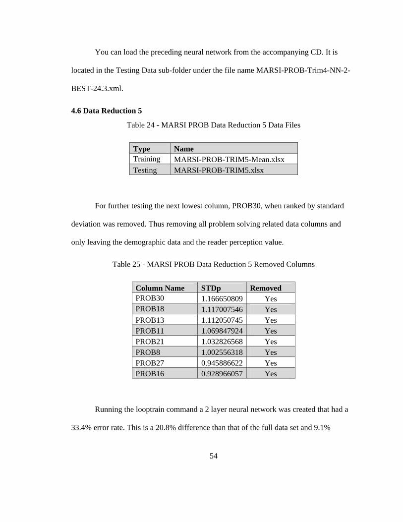
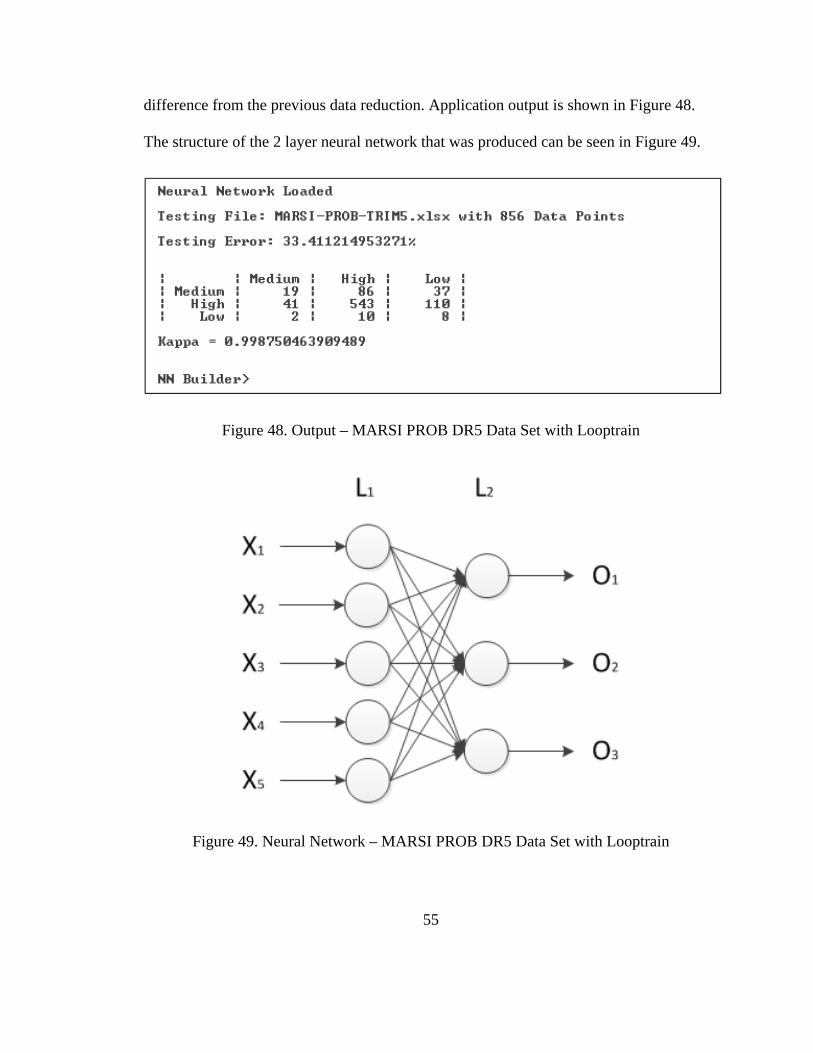
Running the looptrain command a 2 layer neural network was created that had a

33.4% error rate. This is a 20.8% difference than that of the full data set and 9.1%

55

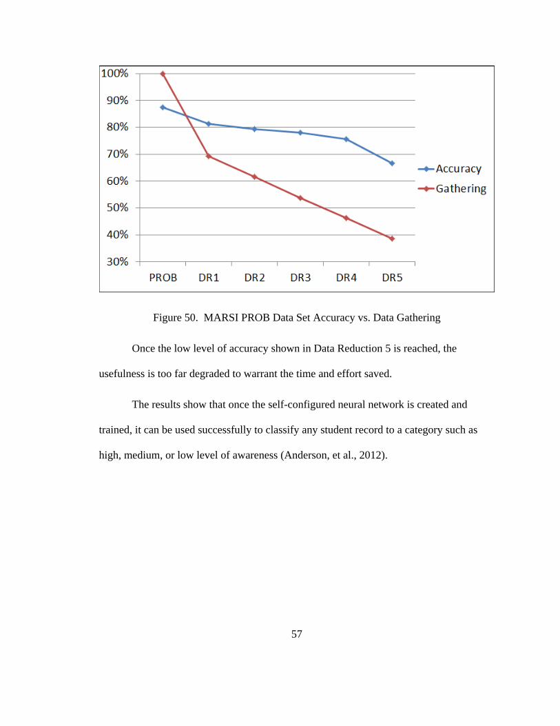
difference from the previous data reduction. Application output is shown in Figure 48.

The structure of the 2 layer neural network that was produced can be seen in Figure 49.

Figure 48. Output – MARSI PROB DR5 Data Set with Looptrain

Figure 49. Neural Network – MARSI PROB DR5 Data Set with Looptrain

56

You can load the preceding neural network from the accompanying CD. It is

located in the Testing Data sub-folder under the file name MARSI-PROB-Trim5-NN-2-

BEST-33.4.xml.

4.7 MARSI Data Set Conclusion

Table 26 - MARSI Results

Data Set Total Columns Best Testing Error MARSI PROB 13 12.62%MARSI PROB DR1 9 18.69%MARSI PROB DR2 8 20.68%MARSI PROB DR3 7 21.96%MARSI PROB DR4 6 24.30%MARSI PROB DR5 5 33.41%

From the results in Table 26 you can see that as the number of data columns is

reduced, so is the overall accuracy. This is a tradeoff that must be given in order to

reduce the data gathering requirements. The selection of the appropriate data model to

use would depend greatly on the study’s requirements and what is an acceptable

accuracy.

Relatively speaking, the difference in overall accuracy of the network created for

Data Reduction 1 and the original network using the full demographic and problem

solving data set is only 6.1%. However it reduced the data gathering requirements by

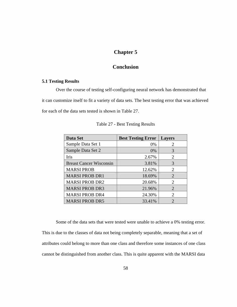
over 30%. In the following chart you can see that this trend continues.

57

Figure 50. MARSI PROB Data Set Accuracy vs. Data Gathering

Once the low level of accuracy shown in Data Reduction 5 is reached, the

usefulness is too far degraded to warrant the time and effort saved.

The results show that once the self-configured neural network is created and

trained, it can be used successfully to classify any student record to a category such as

high, medium, or low level of awareness (Anderson, et al., 2012).

58

Chapter 5

Conclusion

5.1 Testing Results

Over the course of testing self-configuring neural network has demonstrated that

it can customize itself to fit a variety of data sets. The best testing error that was achieved

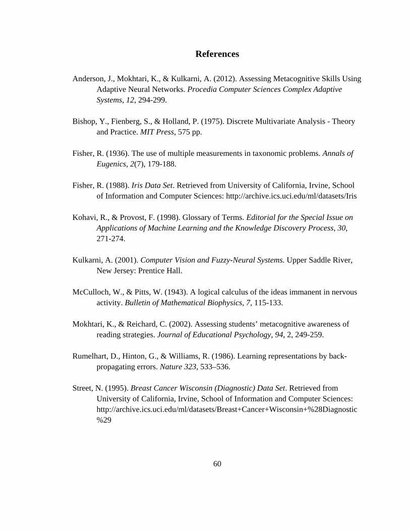
for each of the data sets tested is shown in Table 27.

Table 27 - Best Testing Results

Data Set Best Testing Error Layers Sample Data Set 1 0% 2 Sample Data Set 2 0% 3 Iris 2.67% 2 Breast Cancer Wisconsin 3.81% 3 MARSI PROB 12.62% 2 MARSI PROB DR1 18.69% 2 MARSI PROB DR2 20.68% 2 MARSI PROB DR3 21.96% 2 MARSI PROB DR4 24.30% 2 MARSI PROB DR5 33.41% 2

Some of the data sets that were tested were unable to achieve a 0% testing error.

This is due to the classes of data not being completely separable, meaning that a set of

attributes could belong to more than one class and therefore some instances of one class

cannot be distinguished from another class. This is quite apparent with the MARSI data

59

set and could be due to the nature of the data itself. With the other real world data sets,

the data is measured and repeatable. The MARSI data set, on the other hand, is based off

of a student’s personal feelings about themselves and could vary depending on their

mood and therefore leads to less consistent data.

5.2 Future Work

Adding the ability to execute multiple threads simultaneously would increase this

application’s speed on systems with multi-core CPUs. Each neural node would run in its

own thread and would increase the rate at which data was processed through an existing

network. In addition, multiple training threads could be run at the same time, thus

possibly cutting down on training time.

This application has value in the marketplace. This concept will be further

expanded into an Application Programming Interface (API) and packaging it as a .NET

Dynamic Link Library (DLL). This would allow other programmers to add functionality

from the self-configuring neural network DLL into their own applications. Therefore,

they would be able to take advantage of the accuracy and time savings that a self-

configuring neural network has to offer.

60

References

Anderson, J., Mokhtari, K., & Kulkarni, A. (2012). Assessing Metacognitive Skills Using Adaptive Neural Networks. Procedia Computer Sciences Complex Adaptive Systems, 12, 294-299.

Bishop, Y., Fienberg, S., & Holland, P. (1975). Discrete Multivariate Analysis - Theory and Practice. MIT Press, 575 pp.

Fisher, R. (1936). The use of multiple measurements in taxonomic problems. Annals of Eugenics, 2(7), 179-188.

Fisher, R. (1988). Iris Data Set. Retrieved from University of California, Irvine, School of Information and Computer Sciences: http://archive.ics.uci.edu/ml/datasets/Iris

Kohavi, R., & Provost, F. (1998). Glossary of Terms. Editorial for the Special Issue on Applications of Machine Learning and the Knowledge Discovery Process, 30, 271-274.

Kulkarni, A. (2001). Computer Vision and Fuzzy-Neural Systems. Upper Saddle River, New Jersey: Prentice Hall.

McCulloch, W., & Pitts, W. (1943). A logical calculus of the ideas immanent in nervous activity. Bulletin of Mathematical Biophysics, 7, 115-133.

Mokhtari, K., & Reichard, C. (2002). Assessing students’ metacognitive awareness of reading strategies. Journal of Educational Psychology, 94, 2, 249-259.

Rumelhart, D., Hinton, G., & Williams, R. (1986). Learning representations by back-propagating errors. Nature 323, 533–536.

Street, N. (1995). Breast Cancer Wisconsin (Diagnostic) Data Set. Retrieved from University of California, Irvine, School of Information and Computer Sciences: http://archive.ics.uci.edu/ml/datasets/Breast+Cancer+Wisconsin+%28Diagnostic%29