BULLETIN OF THE POLISH ACADEMY OF SCIENCESTECHNICAL SCIENCESVol. 55, No. 2, 2007

Self-diffusion effects in micro scale liquids. Numerical studyby a dissipative particle dynamics method

J. CZERWIŃSKA∗

Institute of Fundamental Technological Research, Polish Academy of Science, 21 Świętokrzyska St., 00-049 Warsaw, Poland

Abstract. Mesoscale flows of liquid are of great importance for various nano- and biotechnology applications. Continuum modeldo not properly capture the physical phenomena related to the diffusion effects, such as Brownian motion. Molecular approachon the other hand, is computationally too expensive to provide information relevant for engineering applications. Hence, theneed for a mesoscale approach is apparent. In recent years many mesoscale models have been developed, particularly to studyflows of gas. However, mesoscale behaviour of liquid substantially differs from that of gas. This paper presents a numerical studyof micro-liquids phenomena by a Voronoi Dissipative Particle Dynamics method. The method has its origin from the materialscience field and is one of very few numerical techniques which can describe correctly molecular diffusion processes in mesoscaleliquids. This paper proves that correct prediction of molecular diffusion effects plays predominant role on the correct predictionof behaviour of immersed structures in the mesoscopic flow.

Key words: micro- and nanofluidics, mesoscale simulations.

1. Introduction

Reynolds number defines the characteristic of the fluidflow for the continuum medium. If the compressibility ofthe gas was neglected, then gas and liquid can be treatedin similar way. However, from the molecular point of view,the two fluids behave very differently. The average dis-tance between gas molecules is at least one order of mag-nitude higher than in liquids. The interaction in gases ismostly defined by bilateral collisions. In contrary, liquidmolecules are tightly packed and they interact by inter-molecular potential causing cohesion of liquids. Hence, thedifferences between behaviour of liquids and gasses willappear in mesoscale and this leads to requirement for adifferent theoretical and numerical treatments of the twomedia. In the last few years, the research interest hadbeen mostly focused on modelling of micro-flow of gases.Some examples are presented in [1] and [2]. However, theincreasing interest in understanding of bio-processes andthe development of bioengineering requires more compre-hensive study of mesoscale behaviour of liquids. Hence,the present paper will focus on a new numerical develop-ment applicable to liquids.

The question that naturally arises first would be thedefinition of mesoscale. For gases Knudsen number, basedon the molecular mean free path, helps to define bound-aries. Cohesion of liquids, however, makes a counterpartparameter difficult to define. Solids, similarly to liquids,are also characterized by cohesion. Molecules in solids re-main localized in the vicinity of the equilibrium latticeposition (rigidity of solids), and will very rarely jump be-tween neighbours. In liquids molecules will drift apart.

Einstein relation describes the mean square displacementat time t of the molecule from the initial point in timet = 0

< |x(t) − x(0)|2 >= 6 D t, (1)

where D – is self-diffusion parameter. Molecular diffusionis the consequence of the thermal fluctuation and a prop-erty of irreversibility. In contrary to viscous flow, molec-ular diffusion appear spontaneously without presence ofexternal forces, and for liquid, it is typically of the or-der of D ∼ 10−9m2/s. The difference between solids andliquids, which manifests itself in the molecular drift pro-cesses, helps estimate one border of the mesoscale descrip-tion. Due to the fact that molecular diffusion is not limitedby any space or time restriction, this property will definethe upper-bond of the mesoscale. Thermal fluctuations ef-fects (Brownian motion) are prominent on the scale of theorder of micro- and nano-meters. However, on the largerscale and for very long time, the process can be averagedand neglected.

The lower limit of the mesoscale can be derived fromthe differences between gas and liquid at the molecularlevel. The radial distribution function g(r) is a quantita-tive measure of molecular order. It provides the informa-tion about the local density ρ(r) of molecules around agiven molecule. Figure 1 shows radial distribution func-tion for a gas and a liquid. Gas molecules are sparseand bilateral collisions determined transport processes be-tween them. However, liquids on the molecular level arevery different. The radial distribution function has severallocal maxima. This means that behaviour of the singlemolecule is influenced by the closer and also by the rela-

∗e-mail: jczer@ippt.gov.pl

159

J. Czerwińska

tively distant neighbours. The size of the molecules as wellas the strength of the interaction will be limiting factorof various liquid behaviour. Several maxima in radial dis-tribution function can explain the self-organization andclustering mechanism, which occur on the order of nano-meter scale, as illustrated in [3]. By changing the sizeof liquid molecules (polymers, complex molecules in [4])and the strength of interaction (electro-magnetic field in[5]) molecular effects beyond the nano-meter scale have tobe consider. Non-Newtonian behaviour of some liquids isone of the effect connected with the intermolecular scalelength. For most common liquids the changes in theseeffects start to be noticeable on the order of few nano-meters and on the larger scale inter particle interactionsphenomena in liquids are similar to the continuum de-scription. Hence, the intermolecular interaction providesguidelines for the definition of the lower bound of themesoscale.

Fig. 1. Sketch of typical radial distribution function g(r) fora gas and a liquid; σ is the size of the molecule. In liquidsmolecules are tightly packed. Hence, the presence of several

local maxima in the radial distribution function

Concluding, cohesion and molecular drift in liquidsallow the definition of limits on the scale, which laterherein will be referred to as a mesoscale. Molecular de-scription (microscale) is limited by the relevance of thetime and space scales related to the changes in the interparticle potential effects. This describes lower bound ofthe mesoscale. The continuum approach (macroscale) hasits lower bound limited by the influence of the thermalfluctuation phenomena and it provides upper limit of themesoscale. Various phenomena important for the bio- andnanotechnology are taking place in such defined mesoscaleregime. Examples in [6–8]. Due to that fact there is a needfor efficient and accurate simulation techniques which willenhance understanding of mesoscale processes in liquidsas well as provide help in designing micro-devices.

2. Fundamental physics of the mesoscaleliquids

The borders of the mesoscale have been defined in in-troduction section. The lower bound of the scale is es-

tablished by short range changes in intermolecular forceinteraction. However, the interaction is very complex innature and can represent itself in various ways. Neglectingthe possible electromagnetic effects the following phenom-ena are related to the intermolecular potential:

1) interaction between the same fluid molecules – viscouseffects;

2) interaction between molecules of different fluids – im-miscibility, surface tension;

3) interaction between fluid and solid molecules – slip orno-slip phenomena;

4) interaction between two fluids and solid molecules –wetting phenomena.

Fig. 2. Diagram represents comparison of important time andspace scales for liquids. The lines indicate that the consid-ered phenomenon is time dependent on the scale of the orderof femto-seconds, therefore time influence can be neglected;points refer to the specific time and space occurrence of thephenomenon. Indexes on figure represent as follow: 1) Molecu-lar Dynamics study of changes in the surface tension due to thethermal fluctuations (0.9 nm) in [9]; 2) Molecular Dynamicsslip effects in binary mixtures (∼ 2 interaction lengths, 2 nm)in [10]; 3) Molecular Dynamics study of the effect of the rough-ness of the surface on the viscosity of the film (3.89 nm) in [11];4) Molecular Dynamics study of the effect of the length of themolecule on the slip (7.9 nm) in [11]; 5) Molecular Dynam-ics study of the solid-fluid interface boundary condition (upto 10nm) in [12]; 6) Charged colloidal suspension nucleation,self organized structures (320 nm) in [13]; 7) DNA fluctuations(DNA length - 10µm) in [14]; 8) Ecoli RNA fluctuations in [15];9) Colloidal hard spheres suspension in [16]; 10) DNA fluctu-ations (DNA length - 0.1µm) in [17]; 11) Brownian particlesin polymer solutions in [18]; 12) Brownian motion of yeast cell

walls in [19]

Figure 2 shows experimental and numerical data forvarious effects in the mesoscale liquids. The phenomenarelated to the intermolecular forces are generally not timedependant (if time scale is larger than femto-seconds),

160 Bull. Pol. Ac.: Tech. 55(2) 2007

Self-diffusion effects in micro scale liquids. Numerical study by a dissipative particle dynamics method

therefore are marked as a straight lines. The intermolec-ular processes have to be described by microscale (atom-istic) models in the range of several nano-meters. Largerscales do not require such modelling and continuum ap-proach is sufficient. The second type of phenomena relatedto molecular drift will, however, show their strength de-pending on the time and space scale of the problem con-sidered. For complex fluidics such as polymers or colloidsit can be noticeable up to few millimetres. Figure 2 showsthe molecular diffusion effects by dots. Majority of effectswill appear as a Brownian motion of immersed structuresin the flow. It can be noted that some of the data (7–10,12)are correlated as straight line, with the slope being of thevalue of the order of the water diffusion coefficient. Point(11) consider complex polymer colloids. Hence, moleculardiffusion coefficient differs.

In summary, Fig. 2 provides the guideline in decidingthe modelling approach for mesoscale liquids. If the flowphenomena were of the scale larger than several nano-meters, molecular potential interaction is well describedby continuum equations. Molecular drift effects howeverare significant and present on the larger scales. Some phe-nomena such as Brownian motion or molecular mixing areexamples of molecular drift related effects and can showthe influence on various space and time scales. Thus, thetime scale difference in which the intermolecular forcesand self-diffusion phenomena achieve equilibrium statedefines the upper border of the mesoscale. The Schmidtnumber

Sc =ν

D(2)

represents relation of viscous effects (ν -viscosity of fluid)to the mass transfer effects (D self-diffusion). Large Sc(typically for water ∼ 1000) indicate that the equilibriumstate related to the viscous effects is obtained much fasterthan the one corresponding to the molecular drift pro-cesses. Another way to estimate space and time relationlimiting mesoscale physical effects is to define quantitysimilar to the Mach number

M =s/t

a, (3)

where a is speed of sound and instead of the flow velocitythe space s and time t relation of considered problem ispresent. The speed of sound defines the speed of propa-gation of small disturbances in the medium. This can berelated on more fundamental atomic level to the fluctua-tions, example in [20]. Hence if the space and time relationfor a considered problem leads to M ∼ 1, small distur-bances effects will influence the flow. As it can be notedin the characteristic space/time relation from equation 1and from equation 3 for water are of the similar order(7.7 ·10−5 −8.3 ·10−4m/s). Thus, for some circumstancessuch define Mach number maybe easier to estimate thanlocal Schmidt number.

Molecular diffusion will be the predominate factor dif-ferentiating meso- and macroscale. Hence, the numeri-

cal approach to model mesoscale liquids has to describemolecular diffusion processes correctly.

3. Numerical methods and coarsegraining procedure

Mesoscale numerical modelling of liquids requires differ-ent approach from the continuum or molecular simula-tions. Continuum models do not take to account fun-damental phenomenon relevant on such scales such asrandom molecular drift. Molecular simulation, exampleMolecular Dynamics in [21], conceptually also have sev-eral other limitations. The first of which lies in the re-liance of computational part. With the fastest comput-ers to date, the number of liquid molecules reach about10−14 of Avogadro number. Hence, Molecular Dynamicsdescribes very small volume of liquid. The second limita-tion, as indicated by [22], rest on the molecular diffusionprocess itself and the question, if they can be correctlyrepresented by Molecular Dynamics. Thus, restrictions in-dicate that more visible approach is to perform some typesof coarse graining procedure. This can be achieved in sev-eral ways. The most common of which increase the timeand space scales by simplification of interaction properties- Lattice Boltzmann Method in [23]. Generally moleculardiffusion effects are neglected, however some variationsof the Lattice Boltzmann Method allow fluctuation part,example in [24]. Due to the fact, that the motion is re-stricted to the rigidity lattice certain difficulties arise suchas Galilean invariance problem. An alternative approachto coarse graining procedure is to treat the particle as amesocopic object interacting with prescribed interaction- Dissipative Particle Dynamics. The degrees of freedom,which are lost during the coarse graining process, are com-pensated by a respective random forces. This approachwill be presented here and will be described in more de-tails in the next section.

4. Dissipative Particle Dynamicsformulation

The Dissipative Particle Dynamics was originally pro-posed by Hoogerbrugge and Koelman [25] as a combina-tion of Lattice Gas Simulation and Brownian Dynamics.The method is based on the modification of Molecular Dy-namics potential (Lennard-Jones type) from hard spheresto the soft repulsion. This alternation allowed to makelarger time steps possible. However, the removal of thehard core has lead to the drawbacks in modelling vis-cous effects in fluids. The hard core is responsible for thecaging effect. It means that a particle encounters manycollisions before it is transported (similarly like in realfluids). The soft repulsion increases significantly (about1000 times in [27]) mobility of the particles. The Schmidtnumber is Sc ∼1. This implies that viscous time scaleis comparable with the diffusion time scale. Thus, themethod is very inefficient for viscous flows and simulations

Bull. Pol. Ac.: Tech. 55(2) 2007 161

J. Czerwińska

require averaging over significant number of time steps,example in [28] and [29]. Lowe [30] proposed modifica-tion, which allows flow field modelling more efficiently, byusing Maxwellian distribution to strictly control temper-ature and velocity is sampled by Andersen Monte Carlothermostat. This leads to significantly higher viscosityof fluids, hence any Schmidt number can be simulated.However, the low viscosity case becomes difficult to ob-tain using this method. Another drawback of the classicalDissipative Particle Dynamics formulation is that it doesnot include energy equation, thus certain processes can-not be properly modelled. Bonet Avalos and Mackie [31]proposed altered Dissipative Particle Dynamics with en-ergy conservation, however the same problem consider-ing Schmidt number is present and in this case velocitysampling termostat cannot be used. Several other limit-ing factors of classical Dissipative Particle Dynamics needto be mentioned. A small Schmidt number indicates thatthe speed of the propagation of the small disturbances isinvalid (speed of sound is much lower). This will manifestitself in the high speed flows, where the shock wave oc-curs for much lower speeds than in real fluids, but also,it is very important for micro-fluidics. The amplitude ofBrownian motion will be much larger that the one of thereal fluids. Consequently, the average of the flows withimmersed structures are not properly captured. Moreover,the time scale of the Brownian motion for non-equilibriumeffects will be incorrect. As it was mentioned earlier, thesevery phenomena are of the great interest for micro-fluidicsapplications. Next inconvenience is related to the fact thatall dissipative particles are of the same size. The simula-tion of the effects which require various length scales arerestricted by the smallest scale. Hence, this may lead tovery large number of particles. Finally another inconve-nience is connected with the implementation of bound-ary condition. The soft potential allows penetration of aboundary. The introduction of the frozen layer of parti-cles helps in establishing the no-slip wall boundary condi-tion, however it causes clustering of the particles near theboundary. This represents itself as a large density fluctu-ations in the vicinity of the wall (of the order of the valueitself in [28]).

The alternative approach to model fluid is to describea set of volume particles. The origin of this approach is inthe Lagrangian solvers for visco-elastic fluids proposed by[32]. Moving Voronoi mesh describes fluid flow based onthe Navier-Stokes equations. This approach is sufficient,as it was mentioned earlier, to represent all the intermolec-ular related processes (such as viscosity, thermal conduc-tivity). However, molecular drift effects are not taken intoaccount. Hence, additionally fluctuating term has beenadded to ensure a correct value of the molecular diffusioncoefficient. Such formulation has various advantages. Forexample it ensures that the Schmidt number is similar tothat of the real fluids. Moreover, the wall boundary condi-tion can be modelled correctly. There is no density jumpon the wall.

Fig. 3. Voronoi cell i and the quantities defining the discreti-sation algorithm; Aij - length of the edge i j; Rij – distancebetween two particles centres; τij – vector defining changesbetween mass centre of particles i j and the edge centre; ωij –normalized vector indicating relative movement of the centres

of the particles i j; Vi – volume of the particle

Several ways of the derivation of the equations can befound: bottom-up approach in [33] and [34] and top-downderivation in [35,36].

4.1. Basic description – continuum terms. The dis-sipative particle will be defined as a Voronoi cell. Conse-quently, space can be divided completely into conjunctedcells. The density of the particle, in contrary to classi-cal Dissipative Particle Dynamics, will be associated withparticle volume and can be defined as

ρi ≡1Vi

∫Vt

dr ρ(r), (4)

where particle volume is given by relation

Vi ≡∫

Vt

dr. (5)

To discretise a continuum equation into the Voronoi cellsome additional assumptions are needed.

The average of any variable Q is:

[Q]i ≡1Vi

∫Vt

drQ(r). (6)

Following above approximation gradient of variable canbe written as

[∇Q]i =1Vi

∑j

Ωij [Q]j , (7)

where vector Ωij is related to the inter particle mass cen-tre rotation and is given by equation

Ωij ≡ 12Aij ωij . (8)

162 Bull. Pol. Ac.: Tech. 55(2) 2007

Self-diffusion effects in micro scale liquids. Numerical study by a dissipative particle dynamics method

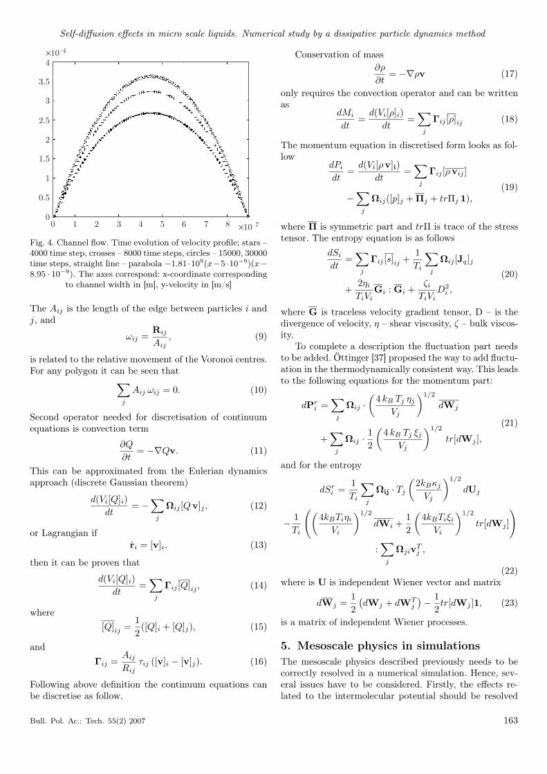
Fig. 4. Channel flow. Time evolution of velocity profile; stars –4000 time step, crosses – 8000 time steps, circles – 15000, 30000time steps, straight line – parabola −1.81 ·109(x−5 ·10−9)(x−8.95 · 10−9). The axes correspond: x-coordinate corresponding

to channel width in [m], y-velocity in [m/s]

The Aij is the length of the edge between particles i andj, and

ωij =Rij

Aij, (9)

is related to the relative movement of the Voronoi centres.For any polygon it can be seen that∑

j

Aij ωij = 0. (10)

Second operator needed for discretisation of continuumequations is convection term

∂Q

∂t= −∇Qv. (11)

This can be approximated from the Eulerian dynamicsapproach (discrete Gaussian theorem)

d(Vi[Q]i)dt

= −∑

j

Ωij [Qv]j , (12)

or Lagrangian ifri = [v]i, (13)

then it can be proven that

d(Vi[Q]i)dt

=∑

j

Γij [Q]ij , (14)

where[Q]ij =

12([Q]i + [Q]j), (15)

andΓij =

Aij

Rijτij ([v]i − [v]j). (16)

Following above definition the continuum equations canbe discretise as follow.

Conservation of mass∂ρ

∂t= −∇ρv (17)

only requires the convection operator and can be writtenas

dMi

dt=

d(Vi[ρ]i)dt

=∑

j

Γij [ρ]ij (18)

The momentum equation in discretised form looks as fol-low

dPi

dt=

d(Vi[ρv]i)dt

=∑

j

Γij [ρvij ]

−∑

j

Ωij([p]j + Πj + trΠj 1),(19)

where Π is symmetric part and trΠ is trace of the stresstensor. The entropy equation is as follows

dSi

dt=

∑j

Γij [s]ij +1Ti

∑j

Ωij [Jq]j

+2ηi

TiViGi : Gi +

ζi

TiViD2

i ,

(20)

where G is traceless velocity gradient tensor, D – is thedivergence of velocity, η – shear viscosity, ζ – bulk viscos-ity.

To complete a description the fluctuation part needsto be added. Öttinger [37] proposed the way to add fluctu-ation in the thermodynamically consistent way. This leadsto the following equations for the momentum part:

dPri =

∑j

Ωij ·(

4 kB Tj ηj

Vj

)1/2

dWj

+∑

j

Ωij ·12

(4 kB Tj ξj

Vj

)1/2

tr[dWj ],

(21)

and for the entropy

dSri =

1Ti

∑j

Ωij · Tj

(2kBκj

Vj

)1/2

dUj

− 1Ti

((4kBTiηi

Vi

)1/2

dWi +12

(4kBTiξi

Vi

)1/2

tr[dWj ]

):∑

j

ΩjivTj ,

(22)where is U is independent Wiener vector and matrix

dWj =12

(dWj + dWT

j

)− 1

2tr[dWj ]1, (23)

is a matrix of independent Wiener processes.

5. Mesoscale physics in simulationsThe mesoscale physics described previously needs to becorrectly resolved in a numerical simulation. Hence, sev-eral issues have to be considered. Firstly, the effects re-lated to the intermolecular potential should be resolved

Bull. Pol. Ac.: Tech. 55(2) 2007 163

J. Czerwińska

properly. As it was noted above for the space scale largerthan 10 nm the continuum approach for such effects issufficient and consistent with experiments. Therefore, asa validation the simulation for the Poiseuille flow was per-formed. For all calculations, the chosen liquid was water.To estimate the parameters of the liquid such as a massof one particle the assumption was made that the dis-tance of the molecules of water in 2-D dissipative particleis the same as in the normal conditions in 3-D volume.From that specific number of molecules was calculated.The channel size was 1500 nm length and 900 nm width.The single dissipative particle here is of the order of 10 nmand the total number of dissipative particles is 10800. Asit can be seen from Fig. 4 the velocity corresponds to thatone of the continuum prediction. It should be emphasizedthat all particles in the flow are shown as the presentationis not a cross-section or result of an averaging procedure.The particles aligned with the flow one behind another,therefore all cross-sections would look identical. The den-sity and entropy, are not plotted, but for this case thereare straight lines with the same constant value and thereis no jump in the vicinity of the wall boundaries. The mainconclusion for this first test is that the continuum scale isresolved correctly even in the range of nano-meters. How-ever, this computations did not involve fluctuation term,which as was indicated earlier is important for mesoscaleliquids.

The influence of the fluctuations on the channel flowcan be seen in Fig. 5a. The plot represents velocity inthe y-direction. The line in the middle refers to the con-tinuum flow for which fluctuation is not included. All re-maining points correspond to the same channel flow withfluctuations. For this case fluctuations in y-velocity arethree orders of magnitude smaller than the velocity in x-direction. Hence, the general velocity profile will not beaffected by fluctuations. However, for smaller flow veloc-ities this tendency will change. Second part of the Fig.5 shows the difference in y-velocity fluctuations for threedifferent channel geometries. First one is as the one above,second is 10 times larger in each direction – 1.5 µm × 0.9µm and the third is 15 µm × 9 µm. As it was expectedBrownian motion of the particles depends on the mass andheavier particles will have smaller fluctuations. Anotherconclusion from the figure is that the centre of the channelseems to be affected less by fluctuations than regions nearthe boundary. This is due to the flow reinforcement andactually will have the influence on the immersed struc-tures behaviour, which will be discussed in details later.

Figure 5 confirms the fact that the Brownian particles(example dissipative particle form computations) moveslower when they are heavier. However, the mean velocityof the drift should stay the same. This is due to the factthat the mean displacement defines self-diffusion coeffi-cient. To estimate the self-diffusion coefficient of the parti-cles another test was performed. Equations 21 and 22 pro-vide information about fluctuation. However, the precisevalue of the term is estimated based on the fluctuation-

dissipation theorem. In macroscopic description it usuallypresents itself as a relation connecting fluctuating termswith dissipative part. Equation 1 can be considered as aone of the very simple example. It connects random fluc-tuations with the macroscopic parameter of self-diffusioncoefficient. Another example of fluctuation-dissipation re-lation is

D =kBT

6πηR, (24)

Fig. 5. Channel flow with fluctuations; a) Velocity in y-direction in the function of y-coordinate, middle line corre-sponds to flow without fluctuations, the dots are representingthe same case with fluctuating term; b) Velocity in y-directionin the function of y-coordinate (normalized to the channelwidth). The middle line represents the largest channel, 15 µm× 9 µm, light points – 1.5 µm × 0.9 µm, black dots – 1200 nm

× 900 nm

which relates random motion to the viscous effects. TheDissipative Particle Dynamics formulation have differentfluctuation-dissipation theorem (details are in [34,35]),

164 Bull. Pol. Ac.: Tech. 55(2) 2007

Self-diffusion effects in micro scale liquids. Numerical study by a dissipative particle dynamics method

which ensures momentum and energy conservation. How-ever, the fluctuation-dissipation theorem also providesseveral other physically significant points. From the mi-croscopic point of view fluctuation will be present inthe system in thermodynamical equilibrium. Onsager hasproven that the system response to the external perturba-tion is correlated with the equilibrium fluctuations. Thediffusion coefficient obtained from studying the equilib-rium correlations is the same as the one in continuummodels for time scale sufficiently longer than relaxationtime. Hence, the fluctuation-dissipation theorem will en-sure that for long time scale the self-diffusion coefficientis constant. Moreover, the speed of sound waves, as a re-sponse of the system to the external perturbation, willalso be controlled by the fluctuation-dissipation theorem.Thus, Eqs. 1 and 3 are indeed representing similar phe-nomena connected to the response of the system to theperturbation. This leads to the realization that correctcalculation of the speed of sound especially on the shorttime scales is crucial for the micro-liquids. To ascertainif the model presented here is correctly behaving in thepresence of disturbance, the following simulation is per-formed. The box 10 µm × 10 µm with 1600 particles ofwater was initially perturbed with small force and thanthe behaviour of the mean particle drift was studied. Fig-ure 6 presents the drift behaviour over time. As it wasexpected in the liquid without fluctuations the diffusioncoefficient based on the particle drift is zero. This occursafter time, when initial disturbance was dumped. The liq-uid with fluctuations behaves differently. Firstly, the veryshort time scale, shows that the motion of the particlesis uncorrelated and its initial rise corresponds to the onewhich is obtained from the simple Langevin equation, ex-ample in [20]. However, longer times lead to correlationbetween particles and this shows in the plateau. For verylong time, however, the constant diffusion coefficient isrecovered. It has to be mentioned, that conservation ofthe mass does not have the fluctuation term. The in-fluence is indirect, through the momentum and entropyequations. Hence, in general the self-diffusion effects canbe estimated correctly without mass exchange betweenparticles. In the simulations one of the curved representsthe behaviour, for particles when mass changes are notallowed. In such a case the diffusion coefficient is largerto compensate mass transfer effects. The diffusion coeffi-cient can be calculated from 24 - 2.19 ·10−14m2/s and forboth cases is in the range of the theoretical prediction forspherical particles (1.85 · 10−14 m2/s; 1.03 · 10−14 m2/s).Hence, the diffusion processes for the small time scales arerepresented correctly by fluctuation-dissipation theoremand for the long time the value is ensured by continuumapproach.

Another aspect which should be considered is if thetime scale between diffusion and viscous process is re-solved correctly. This will be especially important formolecular mixing processes. However, as can be notedfrom the Schmidt number definition 1, if viscosity and

self-diffusion coefficient are known and resolved correctly,the time scale is then estimated correctly.

Fig. 6. Response of the liquid to the small perturbation. (a)two cases, one in which the mass transfer between particles wasnot allowed (higher curve) and second when the mass transferwas present; (b) average mass changes between particles; (c)

the continuum equations without fluctuation term

Finally, after estimating the size of fluctuations andthe relevant time scale, the remaining question is thento ascertain the importance of diffusion processes formesoscale liquids. From the channel flow above with ve-locity Vx = 10−4 m/s and Reynolds number based on the

Bull. Pol. Ac.: Tech. 55(2) 2007 165

J. Czerwińska

channel length Re = 10−4 the size of fluctuation remainsfairly small. Hence, it seems that the fluctuations after allmight not be of primary importance for many engineer-ing applications. The Reynolds number is usually muchlarger and the one of the order of 10−7 would be difficultto obtain. However, this is very misleading. The fluctua-tion impact depends on the space/time scales relation andthe mass of the particle. One of the cases, which is veryinteresting for bioengineering application is the manipu-lation of DNA molecules. As it will be shown below forsuch application self-diffusion effects will influence processsignificantly.

Fig. 7. Channel flow with the DNA chain; a) x-Velocity in thefunction of y-coordinate; all particles are plotted. Main flowmaintain parabolic profile far from the DNA; normalized mass

in the function of y-coordinate; all particles are plotted

5.1. Immersed structures in the flow and Brown-ian effects. A case study to examine the influence of theBrownian effects on the immersed structure is performedby considering the channel flow with DNA chain. Mostof the experimental studies are concerned with stretching

of the DNA, as exemplified in [38–41]. However, here theimportance of the of the flow structures on the stretchingprocess will be underlined. Due to the fact that, the con-sideration are restricted to the estimation of self-diffusioneffects in liquids, the simple model of DNA is sufficientfor such a case study. In general, DNA – fluid interactionis modelled on the atomistic level and the mesoscale de-scription is highly simplified and do not take to accountvarious important phenomena [42]. The mesoscale DNAmodel presented here will be combination of the Dissipa-tive Particle Dynamics and classical FENE approach, andthe way to obtain it is by similar patter as it is performedin the Brownian Dynamics simulations, example in [43].

To model polymer the non-Hookean FENE springmodel was chosen. The force is obeying relation

FFENE =HL

1 − (L/L0)2, (25)

where H is spring constant. The spring cannot extend be-yond L2

0 = 1.2 l2, l is the initial length. The mass centresare associate with every Voronoi centre and the deforma-tion follows similar rules as the one for dissipative particle.

The position of the each bead is calculated simi-larly to the Ermak-McCammon algorithm differentiatingLangevin equation in high friction limit, where inertiaterm are neglected. In our case inertia term will be resultof the DPD integration and will be implicitly influencingbehaviour of the polymer

ri = r0i +

∆t

kT

∑j

D0ij · F0

j + v0i · ∆t, i = 1, .., N. (26)

Generally the chain-solvent interaction is approximatedby the fluctuation part. However, the fluctuation term isnot explicitly present to affect deformation by the velocityof the Dissipative Particle. Such formulation ensures thatdiffusion effects influencing DNA are indeed the same asmodelled in liquid. The diffusion tensor for deformationpart is as presented

D(αβ)0ii =

kT

ζδαβ , i = 1, .., N ;

D(αβ)0ij = 0, i 6= j = 1, .., N ;

(27)

where viscous friction is related to fluid viscosity as

ζ = 6πη 0.257l. (28)

There is another assumption made in considering thestretching mechanism. If the stretched length is muchlonger than the maximum length, the DNA should break.However, in the current simulation, the DNA will stayin fixed position, when stretched to its material propertylimit. The assumption was made to avoid considerationsregarding the material properties in the DNA stretch-ing mechanism. There are several issues considering DNAmodelling, which require detailed studies that are beyondscope of this paper.

To estimate Brownian motion effects following simu-lations were performed. Channel flow 1.2 µm × 0.9 µm

166 Bull. Pol. Ac.: Tech. 55(2) 2007

Self-diffusion effects in micro scale liquids. Numerical study by a dissipative particle dynamics method

with 6300 particles and the DNA is constructed from the87 of Voronoi particles. The Reynolds number based onthe channel length is 6 · 10−5. Accordingly to the Eq. 3the fluctuations will affect time scales around 10−9 s. Atime step was chosen accordingly as 10−10 s, and the totaltime was 4000 time step.

Fig. 8. Velocity distribution in the channel flow during theDNA stretching procedure. The DNA is attached by fixingthe position of the first particle on the left end of the chain.Top picture represents case without fluctuations. Bottom pic-ture shows the same flow with the Brownian effects enhancing

the DNA stretching procedure

Figure 7 presents the example of x-velocity in the func-tion of y-coordinate profile for all particles in the chan-nel. It can be seen that parabolic profile is recovered inthe global channel, as well as in the flow between DNA.The presence of the DNA influences the changes of themass of the particles 7, however the effect is connectedto the numerical error and more information about thiscan be found in the appendix. Figure 8 shows the veloc-ity field for two cases : top one is for without fluctua-tions and the bottom, includes stochastic interaction. Asit can be noted, global velocity field is very similar, how-ever there are significant differences in the vicinity of theDNA chain. The main difference is for non-Brownian flowthe stretching is mostly performed in the direction of theflow. The deformation is smaller, however the stretchinglength is about the same as for the Brownian motion in-fluenced DNA chain. The differences in the behaviour canbe seen even more clearly in Fig. 9. The first part presents

instantaneous resultant x-displacement for every bead ofthe chain. As it can be seen, the Brownian effects increasemovement of the DNA significantly. The second part ofthe figure presents the average displacement of the chainin the flow in the function of time. The average displace-ment should be a function of the mean flow velocity, henceboth curves have similar profile. However, there is signif-icant difference in the behaviour of both cases. The plotcould be considered as a estimation of the diffusion con-stant of the polymer. However, the flow is enforced andthe average displacement also is influenced by the flowitself. Therefore, for the estimation of the diffusion coef-ficient for this case the equation from [42] will be used.The relation between diffusion coefficient of the monomerparticle Dm and polymer chain Dp is

Dp

Dm=

1N

+Rm

Rp, (29)

Fig. 9. The influence of the fluctuations on the DNA stretch-ing procedure; a) the instantienous plot of the x-direction dis-placement for the time 3 · 10−7s as a function of the particlenumber in the chain; stars – correspond to the case withoutfluctuations; circles – displacement with the fluctuations; b)the time evolution of the mean displacement; red, dotted line

– flow without fluctuations, black – flow with fluctuations

Bull. Pol. Ac.: Tech. 55(2) 2007 167

J. Czerwińska

where N is the number of the bead, Rm the radius of themonomer particle, Rp – radius of the polymer. This rela-tion leads for the DNA case to ratio Dp/Dm = 0.048. Thisagain confirms the fact that heavier Brownian particlesis affected by smaller fluctuations. However the averagedisplacement still remains significant, as the DNA-liquidinteraction is reflected in the second part of the equation.Hence, the liquid self-diffusion coefficient will have domi-nating influence on the long polymer chains.

6. ConclusionsThis paper presents a new modelling approach for simu-lating mesoscale phenomena in liquids. As it was shown onsuch a scale the self-diffusion related effects are predomi-nant. Various important nano- and bioengineering appli-cations need to resolve such phenomena, example molec-ular mixing, manipulation of polymers or cells. However,the understanding of following process is still in progress.Experimental approach in some cases, do not providecomplete information. For example, on nano-meter scale,there is difficulty in obtaining the information about theflow field phenomena. Hence, a realistic numerical simula-tion can provide crucial help in bridging the experimentalinformation gap. However, there are very few numericalmethods, which can efficiently cope with this task. Here,the Voronoi Dissipative Particle Dynamics was presentedwith a very satisfying result. The imposing of flux bound-ary condition on the fluid-solid interface and Voronoiadaptivity has significantly reduced density jump on theboundaries, which is present in many particle methodsand which alters significantly flow structure.

Mesoscale phenomena are the resultants of two majoreffects in liquids, namely the intermolecular potential andrandom molecular drift. Both of these aspects help to de-fine the mesoscale borders and also need to be resolvedcorrectly by any numerical approach. Voronoi DissipativeParticle Dynamics, due to the fact that the Schmidt num-ber is similar to that one of the real liquids, models theprocesses accurately and in very efficient way. The pre-sented method, due to the fact that the the time averag-ing is not require to obtain the flow field is few order ofmagnitude faster than other applications of DPD.

It was shown that self-diffusion effects can influenceflow in various ways. In some cases such as channel flow,the fluctuations do not play an important role. However,in the presence of any immersed structure the situationschange drastically. As a example the DNA chain stretch-ing case was chosen. The fluctuation influence alters sig-nificantly this procedure.

Appendix

Numerical procedure, accuracyand efficiency.There are several issues related to the numerical proce-dure. First is related to the movement of the Voronoi

lattice. Voronoi diagram is a tool to describe proximityof neighbouring points U = P1, ..., Pn. The perpendicularbisector is defined as

Bij = x ∈ <2 | d(x, Pi) = d(x, Pj) , (A1)

where d(x, Pi) is the distance between any point x andVoronoi center Pi. The Voronoi polygon of Pi is definedas

V (Pi) = x ∈ <2 | ∀i 6=j d(x, Pi) ≤ d(x, Pj) . (A2)

Set of Voronoi points defines Voronoi diagram, dual graphto the Delaunay triangulation. Due to the movement ofVoronoi centres the diagram requires reconstruction. Twoassumptions are important: first that points do not col-lide and second that initial diagram is actually a Voronoidiagram. In such a case there are three types of events.The appearance (or disappearance) of additional Voronoipoint in the neighbouring vicinity of point Pi. If the pointPi is on the wall, therefore does not move or is on theperiodic boundary, in such case the mirror image of pointPi is created. Therefore the problem is confined to consid-eration of movement of the Voronoi lattice on the torus.It can be shown that the change in the Voronoi lattice ischaracterized by topological diagram shown in Fig. 11.

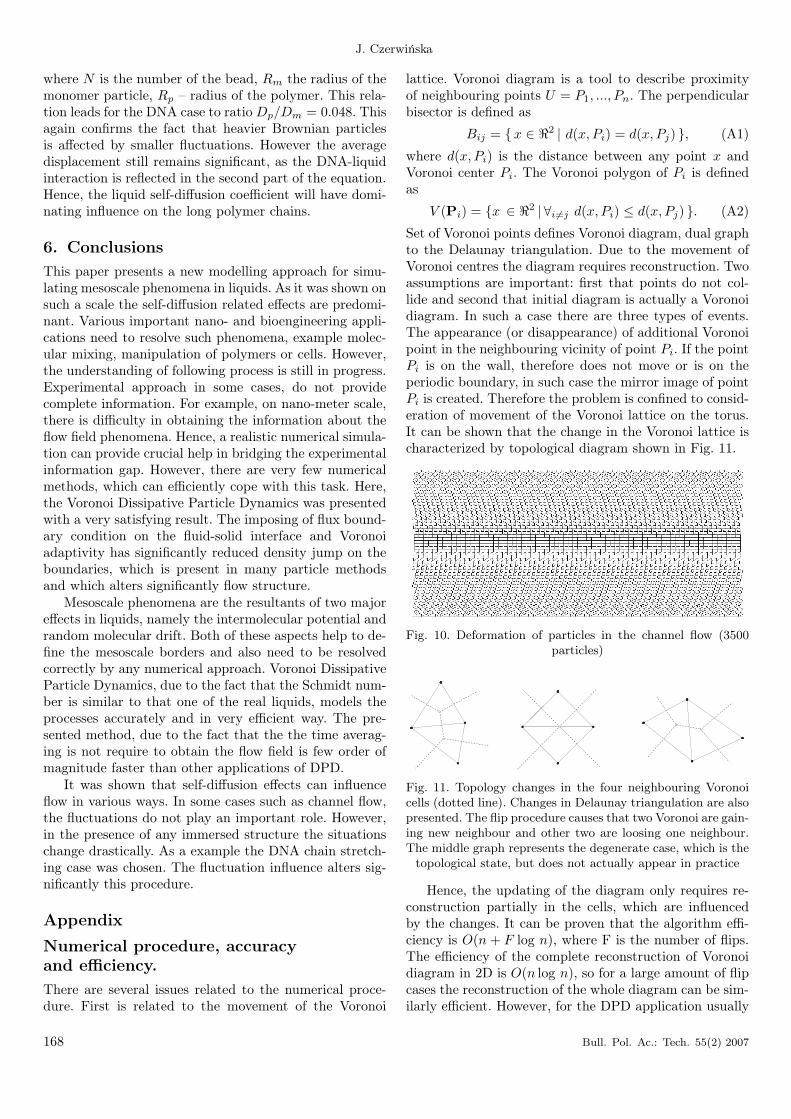
Fig. 10. Deformation of particles in the channel flow (3500particles)

Fig. 11. Topology changes in the four neighbouring Voronoicells (dotted line). Changes in Delaunay triangulation are alsopresented. The flip procedure causes that two Voronoi are gain-ing new neighbour and other two are loosing one neighbour.The middle graph represents the degenerate case, which is the

topological state, but does not actually appear in practice

Hence, the updating of the diagram only requires re-construction partially in the cells, which are influencedby the changes. It can be proven that the algorithm effi-ciency is O(n + F log n), where F is the number of flips.The efficiency of the complete reconstruction of Voronoidiagram in 2D is O(n log n), so for a large amount of flipcases the reconstruction of the whole diagram can be sim-ilarly efficient. However, for the DPD application usually

168 Bull. Pol. Ac.: Tech. 55(2) 2007

Self-diffusion effects in micro scale liquids. Numerical study by a dissipative particle dynamics method

time step is limited by entropy grow and the changes ofparticles size are small, requires very few flips (less than5%) in every time step.

More details about the construction of moving Voronoidiagram can be found in [44].

Fig. 12. Mass change due to the Voronoi lattice motion

Fig. 13. DNA in the channel flow. Changes in density due tothe adaptation of the volume of the particles to the flow struc-

tures

The example of the particle deformation in a chan-nel flow is given in figure 10. It should be noted that themovement of the particles depends on the flow velocity.Thus, for a given geometry, in some cases the mesh willdeform more and in other cases, they will stay mostlyin the original position. The original mesh is build fromequally distributed points, which are slightly perturbatedto obtain Voronoi diagram. In the case of channel flowspresented in the paper the mesh did not deform notice-ably. The disadvantage of the deformation is that the ac-curacy of the integration is lower and the numerical errorincreases. Example is given for the channel flow, for thesame channel geometry which was considered for DNAflow, except that DNA chain is not present. The time is4 times longer than DNA simulation. Figure 12 presentschanges in the normalized mass of the particles in the

presence of extensive motion. It needs to be indicated thatit is strictly numerical error and can be reduced to anysmall value by reducing the time step size. However, forthe flow with the DNA chain the extensive deformationmakes the changes in the DNA position faster. Hence, thecompromise has to be determined between accuracy re-quirement and the desired speed of considered process.Next computational issue is related to the boundary con-ditions. Classical Dissipative Particle Dynamics representno-slip boundary condition with the frozen particle layer.However, it leads to clustering of particles in the vicinityof the boundaries and this is responsible for large den-sity jump. To model wall boundary condition also frozenparticles layer was assumed. However, the mass exchangebetween particles is allowed, as does entropy change. Thisleads to very different result than the one obtained inmany particle methods. The boundary is represented ac-curately, and there is no density jump. However, whenthe immersed structures are present, some complex flowpatters cause density changes. The mass as it was shownin Fig. 7b) does not change significantly, but the volumeof the particles does. This can be seen in Fig. 13. This nu-merical inconvenience can be reduced by imposing certainrules on the particle splitting or creation in the vicinityof stagnation and wake region.

Another computational issue is related to the chan-nel flow, for which periodic boundary conditions wereimposed and the flow was driven by the force. Periodicboundary is represented in the way that the Voronoi edgenodes have the same index, however two different actualpositions. The nodes, however have one position and onlycommunicate fact that some neighbours may have distantposition. This leads to the fact, that there are no extraghosts cells in the system and all particle seen on figuresare indeed the all particles of the fluid.

Finally, remaining issue considers time integrationand algorithm efficiency. For the time integration Runge-Kutta method was used. Due to the fact that the Schmidtnumber is of the same order as real fluids, stochastic partin many cases is very small. Hence, the integration errorfor that part is small as well. In the case when the fluctu-ation term is larger the appropriate stochastic integrationscheme should be used. The stability of the algorithm isestimated by the two factors Γij and Ωij . Parameter Γij

indicates changes in the shape of the Voronoi cells, whileΩij is related to the relative movement of the mass cen-tres of two interacting particles. Due to the fact that theconservation of mass 18 needs to be fulfilled with as smallerror as possible the parameter Γij will restrict the timestep. Reversible part will be determining the time step,also when the irreversible processes are present. How-ever, parameter Ωij determines how many time steps areneeded to obtain fully developed flow profile. Hence, thedifference between these two parameters is responsible forthe fact that in some cases the mesh moves extensivelyand in some the flow can be established without notice-able deformation of Voronoi lattice.

Bull. Pol. Ac.: Tech. 55(2) 2007 169

J. Czerwińska

Time efficiency can be also studied from the differ-ent aspect. Schmidt number has influence not only onthe physical aspect of the flow. It determines how easilythe flow structures can be obtained. In case presented in[28] to obtain channel flow 2.5 107 timesteps were needed(2500 timesteps and every time step was averaged over104 timesteps) with the calculations performed withoutenergy conservation. The energy equation makes parti-cles more mobile, example in [29] and requires even longeraveraging. Here, however the flow in some cases can beobtained after as low as 4000 timesteps with the sameamount of particles (10800) and this include energy equa-tion. Thus, despite of inconvenience in requirement forthe move of the complex geometrical structures such asVoronoi cells, the method is very time efficient.

References

[1] M. Gad-el-Hak, “The fluid mechanics of microdevices thefreeman scholar lecture”, J. Fluids Eng. 121, 533 (1999).

[2] H. Herwig, “Flow and heat transfer in micro systems: iseverything different or just smaller?”, Z. Angew. Math.Mech. 82, 579586 (2002).

[3] K. Pohl, M.C. Bartelt, J. de la Figuera, N.C. Bartelt, J.Hebek, and R.Q. Hwang, “Identifying the forces responsi-ble for self-organization of nanostructures at crystal sur-faces”, Nature 397, 238241 (1999).

[4] W. Dzwinel and D. A. Yueny, “A two-level, discrete-particle approach for simulating ordered colloidal struc-tures”, J. Coll. Interf. Sc. 225, 179190 (2000).

[5] I. Aranson, S.B. Meerson, P.V. Sasorov, and V.M. Vi-nokur, “Phase separation and coarsening in electrostati-cally driven granular media”, Phys. Rev. Lett. 88, 204301–204314 (2002).

[6] A.A. Darhuber and S.M. Troian, “Principles of microflu-idic actuation by modulation of surface tension”, Annu.Rev. Fluid Mech. 37, 425455 (2005).

[7] C.-M. Ho and Y.-C. Tai, “Micro-electro-mechanical-systems (MEMS) and fluid flows”, Annu. Rev. FluidMech. 30, 579612 (1998).

[8] H.A. Stone, A.D. Stroock, and A. Ajdari, “Engineeringflows in small devices: microfluidics towards a lab-on-a-chip”, Annu. Rev. Fluid Mech. 36, 381411 (2004).

[9] S. Senapati and M.L. Berkowitz, “Computer simulationstudy of the interface width of the liquid /liquid inter-face”, Phys. Rev. Lett. 87 (17), 176101–176114, (2001).

[10] C. Denniston and M. O. Robbins, “Molecular and con-tinuum boundary conditions for a miscible binary fluid”,Phys. Rev. Lett. 87 (17), 178302–178314 (2001).

[11] A. Jabbarzadeh, J.D. Atkinson, and R. I. Tanner, “Effectof the wall roughness on slip and rheological properties ofhexadecane in molecular dynamics simulation of Couetteshear flow between two sinusoidal walls”, Phys. Rev. E 61(1), 690699 (2000).

[12] M. Cieplak, J. Koplik, and J.R. Banavar, “Boundary con-ditions at a fluid-solid interface”, Phys. Rev. Lett. 86 (5),803806 (2001).

[13] M. Knott and I.J. Ford, “Surface tension and nucleationrate of phases of a charged colloidal suspension”, Phys.Rev. E 65, 061401–061413, (2002).

[14] D.E. Smith, H. P. Babcock, and S. Chu, “Single-polymer

dynamics in steady shear flow”, Science 283, 17241727(1999).

[15] R.J. Davenport, G.J.L. Wuite, R. Landick, and C. Bus-tamante, “Single-molecule study of transcriptional paus-ing and arrest by E. coli RNA polymerase”, Science 287,24972500 (2000).

[16] W.K. Kegel and A. van Blaaderen, “Direct observationof dynamical heterogeneities in colloidal hard-sphere sus-pensions”, Science 287, 290293 (2000).

[17] D. Nykypanchuk, H.H. Strey, and D.A. Hoagland, “Brow-nian motion of DNA confined within a two-dimensionalarray”, Science 297, 987990 (2002).

[18] J. van der Gucht, N.A.M. Besseling, W. Knoben, L.Bouteiller, and M.A. Cohen Stuart, “Brownian particlesin supramolecular polymer solutions”, Phys.Rev. E 67,051106–051110 (2003).

[19] A.E. Pelling, S. Sehati, E.B. Gralla, J.S. Valentine,and J.K. Gimzewski, “Local nanomechanical motion ofthe cell wall of Saccharomyces Cerevisiae”, Science 305,11471150 (2004).

[20] J.-L. Barrat and J.-P. Hansen, Basic Concepts for Simpleand Complex Liquids, Univ. Press, Cambridge, 2003.

[21] P. Koumoutsakos, “Multiscale flow simulations using par-ticles”, Annu. Rev. Fluid Mech. 37, 457487 (2005).

[22] H. Brenner, “Is the tracer velocity of a fluid continuumequal to its mass velocity?”, Phys. Rev. E 70, 061201–061210 (2004).

[23] S. Chen and G.D. Doolen, “Lattice Boltzmann method forfluid flows”, Annu. Rev. Fluid Mech. 30, 329364 (1998).

[24] A.J.C. Ladd, “Short time motion of colloidal particles:Numerical simulations via a fluctuating lattice Boltz-mann equation”, Phys. Rev. Lett. 70, 1330–1342 (1993).

[25] P.J. Hoogerbrugge and J.M.V.A. Koelman, “Simulatingmicroscopic hydrodynamics phenomena with dissipativeparticle dynamics”, Europhys. Lett. 19, 155160 (1992).

[26] C.L. Henry, C. Neto, D.R. Evansa, S. Biggs, and V.S.J.Craig, “The effect of surfactant adsorption on liquidboundary slippage”, Physica A 339, 6065 (2004).

[27] R.D. Groot, “Application of dissipative particle dynam-ics”, Lect. Notes Phys. 640, 538 (2004).

[28] X. Fan, N. Phan-Thien, N.T. Yong, X.Wu, and D. Xu,“Microchannel flow of a macromolecular suspension”,Phys. Fluids 51, 1121 (2003).

[29] U. Salecker, J. Czerwinska, N.A. and Adams, “Modellingof micro-cavity flow ba a Dissipative Particle Dynamicsmethod”, Proceed. GAMM (2004).

[30] C.P. Lowe, “Alternative approach to dissipative particledynamics”, Europhys. Lett. 47, 145151 (1999).

[31] J. Bonet Avalos and A.D. Mackie, “Dissipative particledynamics with energy conservation”, Europhys. Lett. 40,141146 (1997).

[32] X.F. Yuan, R.C. Ball, and S.F. Edwards. “A new ap-proach to modelling voscpelastic fluid flows”, J. Non-Newtonian Fluid Mech. 46, 331350 (1993).

[33] E.G. Flekkøy and P. V. Coveney, “From Molecular Dy-namics to Dissipative Particle Dynamics”, Phys. Rev.Lett. 83, 17751778 (1999).

[34] E.G. Flekkøy, P.V. Coveney, and G. De Fabritiis, “Foun-dations of dissipative particle dynamics”, Phys. Rev. E62, 21402157(2000).

[35] M. Serrano, G. De Fabritiis, P. Español, E. G. Flekkøy,and P.V. Coveney, “Mesoscopic dynamics of Voronoi fluid

170 Bull. Pol. Ac.: Tech. 55(2) 2007

Self-diffusion effects in micro scale liquids. Numerical study by a dissipative particle dynamics method

particles”, J. Phys. A: Math. Gen. 35, 16051625 (2002).[36] M. Serrano and P. Español, “Thermodynamically consis-

tent mesoscopic fluid particle model”, Phys. Rev. E 64,046115–046118 (2001).

[37] H. C. Öttinger, “General projection operator formalismfor the dynamics and thermodynamics”, Phys. Rev. E 57,1416 (1999).

[38] A. Crut, D. Lasne, J.-F. Allemand, M. Dahan, andP. Desbiolles, “Transverse fluctuations of single DNAmolecules attached at both extremities to a surface”,Phys.Rev. E 67, 051910-051916 (2003).

[39] P.S. Doyle, E.S.G. Shaqfeh, and A. P. Gast, “Dynamicsimulation of freely draining flexible polymers in steadylinear flows”, J. Flid Mech. 334, 251291 (1997).

[40] R.M. Jendrejack, E.T. Dimalanta, D.C. Schwartz, M.D.Graham, and J.J. de Pablo, “DNA dynamics in a mi-crochannel”, Phys. Rev. E 91 (3), 038102-038114 (2003).

[41] B. Ladoux and P. S. Doyle, “Stretching tethered DNAchains in shear flow”, Euro Phys. Lett. 52, 511517 (2000).

[42] C.P. Lowe and M.W. Dreischor, “Simulating the dynamicsof the mesoscopic systems”, Lett. Notes Phys. 640, 3968(2004).

[43] A.V. Lyulin, D.B. Adolf, and G.R. Davies, “Brownian dy-namics simulations of linear polymers under shear flow”,J. Chem. Phys. 111 (2), 758771 (1999).

[44] G. Albers, J.S.B. Mitchell, L.J. Guibas, and T. Roos,“Voronoi diagram of moving points”, 3rd SWAT 92 (1992).

Bull. Pol. Ac.: Tech. 55(2) 2007 171