University of South Florida University of South Florida Scholar Commons Scholar Commons Graduate Theses and Dissertations Graduate School 11-14-2003 Self-interference Handling in OFDM Based Wireless Self-interference Handling in OFDM Based Wireless Communication Systems Communication Systems Tevfik Yücek University of South Florida Follow this and additional works at: https://scholarcommons.usf.edu/etd Part of the American Studies Commons Scholar Commons Citation Scholar Commons Citation Yücek, Tevfik, "Self-interference Handling in OFDM Based Wireless Communication Systems" (2003). Graduate Theses and Dissertations. https://scholarcommons.usf.edu/etd/1511 This Thesis is brought to you for free and open access by the Graduate School at Scholar Commons. It has been accepted for inclusion in Graduate Theses and Dissertations by an authorized administrator of Scholar Commons. For more information, please contact [email protected].
Transcript
University of South Florida University of South Florida
Scholar Commons Scholar Commons
Graduate Theses and Dissertations Graduate School
11-14-2003
Self-interference Handling in OFDM Based Wireless Self-interference Handling in OFDM Based Wireless
Communication Systems Communication Systems
Tevfik Yücek University of South Florida
Follow this and additional works at: https://scholarcommons.usf.edu/etd
Part of the American Studies Commons
Scholar Commons Citation Scholar Commons Citation Yücek, Tevfik, "Self-interference Handling in OFDM Based Wireless Communication Systems" (2003). Graduate Theses and Dissertations. https://scholarcommons.usf.edu/etd/1511
This Thesis is brought to you for free and open access by the Graduate School at Scholar Commons. It has been accepted for inclusion in Graduate Theses and Dissertations by an authorized administrator of Scholar Commons. For more information, please contact [email protected].
4.3.6.1 Cancellation in modulation 574.3.6.2 Cancellation in demodulation 584.3.6.3 A diverse self-cancellation method 60
4.3.7 Tone reservation 614.4 ICI cancellation using auto-regressive modeling 62
4.4.1 Algorithm description 624.4.1.1 Auto-regressive modeling 624.4.1.2 Estimation of noise spectrum and whitening 63
4.4.2 Performance results 644.5 Conclusion 65
CHAPTER 5 ICI CANCELLATION BASED CHANNEL ESTIMATION 665.1 Introduction 665.2 System model 675.3 Algorithm description 67
5.3.1 Properties of interference matrix 685.3.2 Channel frequency correlation for choosing the best hypothesis 695.3.3 The search algorithm 705.3.4 Reduced interference matrix 71
5.4 Results 725.5 Conclusion 75
CHAPTER 6 CONCLUSION 76
REFERENCES 78
ii
LIST OF FIGURES
Figure 1. Basic multi-carrier transmitter. 2
Figure 2. Power spectrum density of transmitted time domain OFDM signal. 7
Figure 3. Power spectrum density of OFDM signal when the subcarriers at the sidesof the spectrum and at DCis set to zero. 8
Figure 4. Illustration of cyclic prefix extension. 9
Figure 5. Responses of different low-pass filters. 11
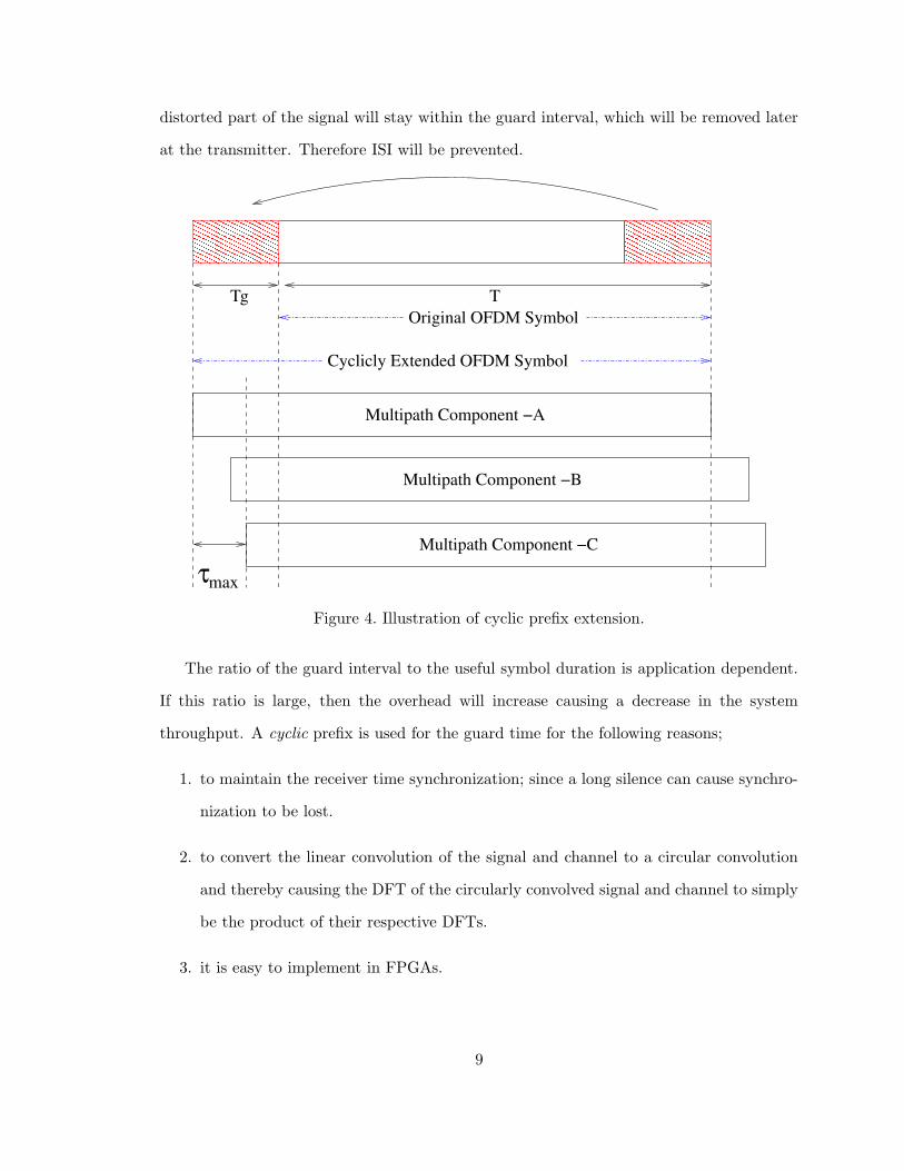
Figure 6. Spectrum of an OFDM signal with three channels before and after band-pass filtering. 12
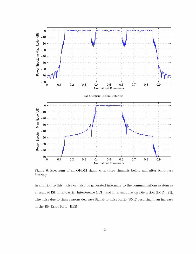
Figure 7. An example 2D channel response. 14
Figure 8. Block diagram of an OFDM transceiver. 15
Figure 9. Moose’s frequency offset estimation method. 16
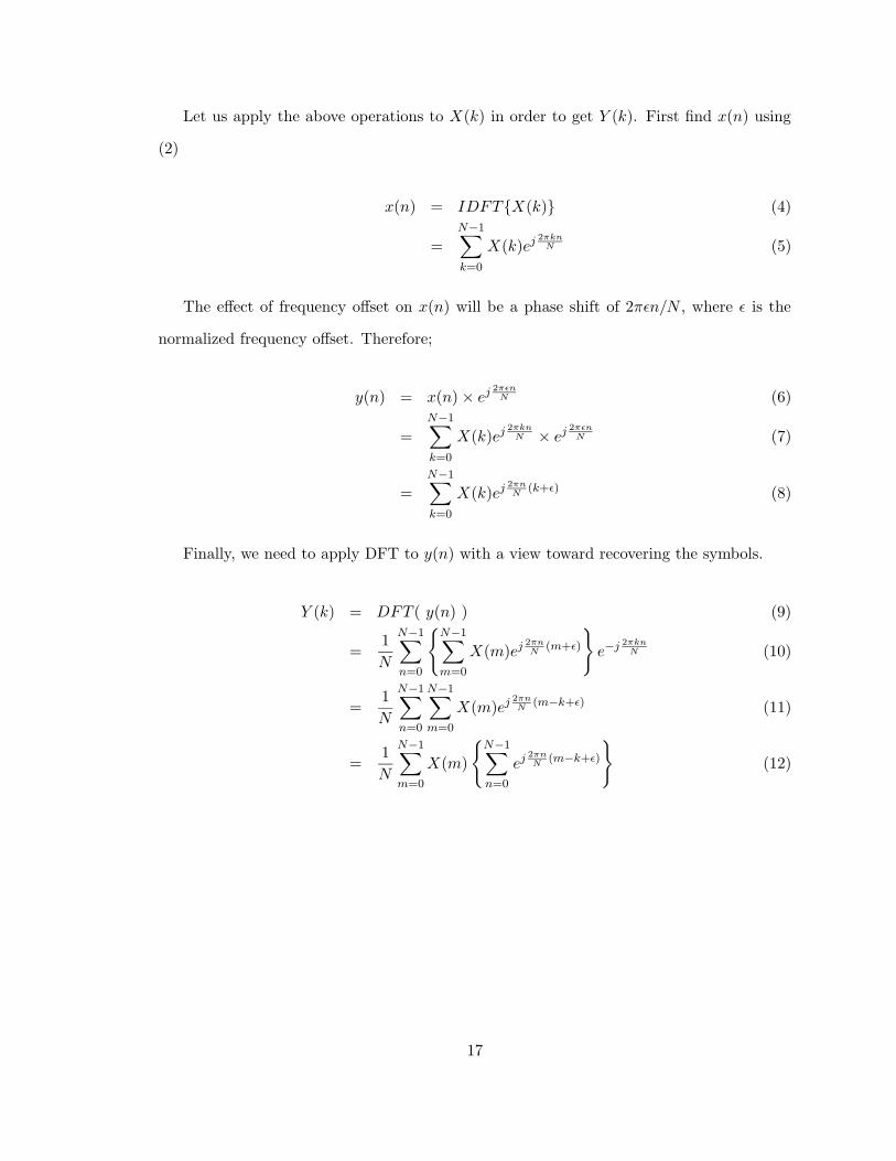
Figure 10. Constellation of received symbols when 5% normalized frequency offset ispresent. 19
Figure 11. The probability that the magnitude of the discrete-time OFDM signalexceeds a threshold x0 for different modulations. 25
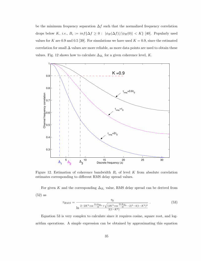
Figure 12. Estimation of coherence bandwidth Bc of level K. 35
Figure 13. RMS delay spread versus coherence bandwidth. 36
Figure 14. Sampling of channel frequency response. 42
Figure 15. Normalized mean squared error versus channel SNR for different samplingintervals. 43
Figure 16. Comparison of the estimated frequency correlation with the ideal correla-tion for different RMS delay spread values. 44
Figure 17. Normalized mean-squared-error performance of RMS delay spread estima-tion for different averaging sizes. 45
Figure 18. Different power delay profiles that are used in the simulation. 46
iii
Figure 19. Normalized mean-squared-error performance of RMS delay spread estima-tion for different power delay profiles. 47
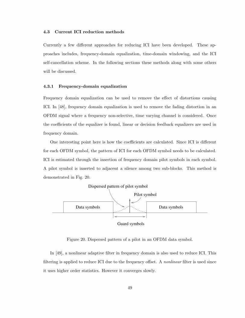
Figure 20. Dispersed pattern of a pilot in an OFDM data symbol. 49
Figure 21. Position of carriers in the DFT filter bank. 51
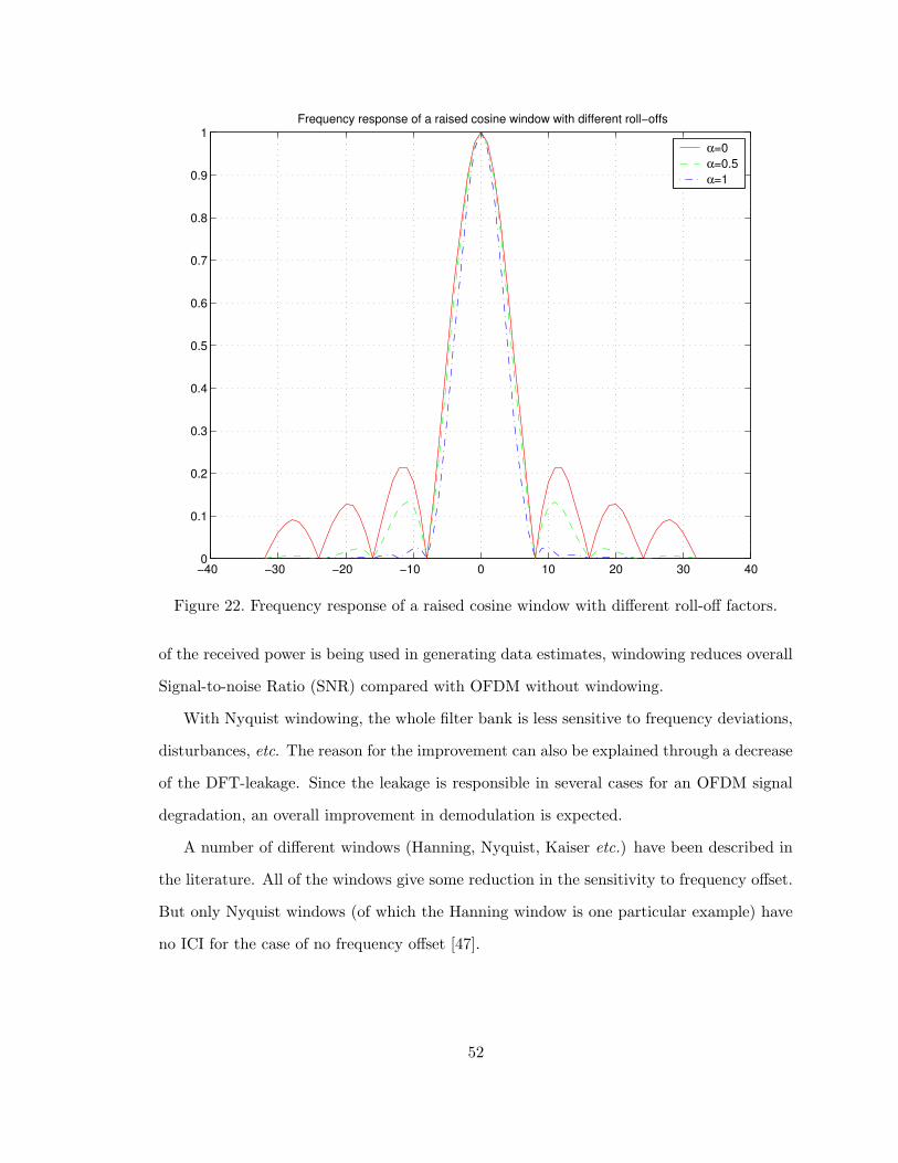
Figure 22. Frequency response of a raised cosine window with different roll-off factors. 52
Figure 23. All possible different signal constellation for 4-ZPSK. 56
Figure 24. Real and imaginary parts of ICI coefficients for N=16. 57
Figure 25. Comparison of K(m, k), K ′(m, k) and K ′′(m, k). 59
Figure 26. Power spectral density of the original and whitened versions of the ICIsignals for different AR model orders. 64
Figure 27. Performance of the proposed method for different model orders. ε = 0.3. 65
Figure 28. Magnitudes of full and reduced interference matrices for different fre-quency offsets. 72
Figure 29. Variance of the frequency offset estimator. 73
Figure 30. Estimated and correct (normalized) frequency offset values. 74
Figure 31. Mean-square error versus SNR for conventional LS and proposed CFRestimators. 75
iv
LIST OF ACRONYMS
ACI Adjacent Channel Interference
ADSL Asymmetric Digital Subscriber Line
AR Auto-regressive
AWGN Additive White Gaussian Noise
BER Bit Error Rate
BPSK Binary Phase Shift Keying
CCI Co-channel Interference
CFC Channel Frequency Correlation
CFR Channel Frequency Response
CIR Channel Impulse Response
DAB Digital Audio Broadcasting
DC Direct Current
DFE Decision Feedback Equalizer
DFT Discrete Fourier Transform
DVB-T Terrestrial Digital Video Broadcasting
FFT Fast Fourier Transform
FPGA Field-Programmable Gate Array
GSM Global System for Mobile Communications
ICI Inter-carrier Interference
IDFT Inverse Discrete Fourier Transform
IEEE Institute of Electrical and Electronics Engineers
Figure 13. RMS delay spread versus coherence bandwidth. The approximation and actualresults are shown for two different coherence levels, K=0.5 and K=0.9.
36
Some relations between coherence bandwidth and RMS delay spread is also defined
in [39, 40]. The true relationship between Bc and τRMS is an uncertainty relationship and
is given in [40] as
Bc ≥cos−1 K
2πτRMS(55)
which can also be written as
BcτRMS ≥ cos−1 K
2π, (56)
putting a lower bound on the product of coherence bandwidth and RMS delay spread. The
values of the constant C, which is obtained by simulation, is found to be always above this
lower limit.
3.3.3 Effect of impairments
3.3.3.1 Additive noise
Additive noise is one of common limiting factors for most algorithms in wireless communi-
cations and it is often assumed to be white and Gaussian distributed. In our system model
we have also made the same assumptions. The effect of noise on the CFC is given in (42),
where it appears as a DC term whose magnitude depends on noise variance. Extrapolation
is used to calculate the actual value of DC term using the correlation values around DC
value. This way, some inherent information about the channel SNR can also be obtained.
Inter-carrier Interference (ICI) is biggest impairment in OFDM systems which can be
caused by carrier frequency offset, phase noise, Doppler shift, multipath, symbol timing
errors and pulse shaping. It is commonly modeled as white Gaussian noise [41, 42], and
considered as part of AWGN.
3.3.3.2 Carrier-dependent phase shift in channel
Timing offset is another impairment in OFDM which is also folded into the channel. It
introduces a sub-carrier dependent phase offset on the channel [43, 44]. Channel frequency
37
response that includes the effect of timing offset can be written as
Hm(k) = Hm(k)e−j 2πkθN , (57)
where θ is time offset value.
Using (57), CFC in the presence of timing error can be calculated as
φH(∆) = Em,k{Hm(k)H∗m(k + ∆)}
= φH(∆)e−j 2π∆θN . (58)
This equation shows that timing error causes a constant phase shift in the CFC. However,
this does not affect the proposed algorithm since the magnitude of CFC, which is not
affected from timing offset, is used.
3.4 Short term parameter estimation
In the previous sections, an algorithm to find the global parameters of wireless channel
were described. However, some applications may require instantaneous parameters for
adaptation. Especially, in low mobility scenarios, where wireless channel does not change
frequently, instantaneous channel parameters should be used. In this section, a method for
obtaining the instantaneous channel parameters in a computationally effective way by using
the CFR is explained and the effects of OFDM impairments on this method are discussed.
Time domain parameters, e.g. RMS delay spread, can be calculated if CIR is known.
Therefore, we will concentrate on the calculation of CIR effectively in the next section.
3.4.1 Obtaining CIR effectively
Channel frequency response for an OFDM system can be calculated using DFT of time
domain CIR. Assuming that we have an L tap channel, and the value of lth tap for the mth
38
OFDM symbol is represented by hm(l). Then CFR can be found as
Hm(k) =1
N
N−1∑
l=0
hm(l)e−j2πkl/N 0 ≤ k ≤ N − 1 . (59)
The reverse operation can be done as well, i.e. CIR can be calculated from CFR with IDFT
operation.
Channel estimation in frequency domain is studied extensively for OFDM systems [45,
46]. We can use estimated CFR of received samples, (40), to calculate time domain CIR.
This method is used in [11] to obtain the coefficients of channel estimation filter adaptively.
However, it requires IDFT operation with a size equal to the number of subcarriers.
CFR can be sampled to reduce the computational complexity. In this case, we need to
sample CFR according to Nyquist theorem in order to prevent aliasing in time domain. We
can write this as
τmax∆fSf ≤ 1 , (60)
where τmax is maximum excess delay of the channel, ∆f is subcarrier spacing in frequency
domain, and Sf is the sampling interval. Note that the right hand side of the above equation
is 1 and not 1/2. This is because PDP is nonzero between 0 and τmax. We can represent
frequency spacing in terms of OFDM symbol duration (∆f = 1/Tu), then we can re-write
(60) as
τmax ≤ Tu
Sf. (61)
From the above equation by assuming worst case maximum excess delay, sampling rate
can easily be calculated. Alternatively, sampling rate can also be adaptively calculated by
using maximum excess delay calculated in the previous steps instead of using the worst case
maximum excess delay of the channel.
39
Using (40) and (59), estimate of CFR can be written as
Hm(k) = Hm(k) + Wm(k)
=1
N
L−1∑
l=0
hm(l)e−j2πkl/N + Wm(k) , (62)
where Wm(k) are independent identically distributed complex Gaussian noise variables.
Note that we have replaced the upper bound of summation with L − 1 since hm(l) is zero
for l ≥ L.
The CFR estimate is sampled with a spacing of Sf . The sampled version of the estimate
can, then, be written as
H ′m(k) =
1
N
L−1∑
l=0
hm(l)e−j2π(Sf k)l/N + Wm(Sfk) 1 ≤ k ≤ N
Sf. (63)
Without loss of generality, we can assume NSf
= L. Now, CIR can be obtained by
taking IDFT of the sampled estimate CFR. IDFT size is reduced from N to N/Sf by using
sampling. As a result of this reduction, the complexity of the IDFT operation will decrease
at least Sf times. For wireless LAN (IEEE 802.11a), for example, the worst case scenario
Sf would be 4 (assuming a maximum excess delay equal to guard interval, 0.8µs), which
decreases original complexity by at least 75 percent.
An IDFT of size N/Sf = L is applied to (63) in order to obtain the estimate of CIR as
hm(l) = IDFT
{
1
N
L−1∑
n=0
hm(n)e−j2πkn/L + Wm(Sfk)
}
= hm(l) + w′
m(l) , (64)
where w′
m(l) is the IDFT of the noise samples.
Equation 64 gives the instantaneous CIR. Having this information, PDP can be calcu-
lated by averaging the magnitudes of instantaneous CIR over OFDM symbols.
40
Channel estimation error will result in additive noise on the estimated CIR. The signal-
to-estimation error ratio for CIR will be equal to signal-to-estimation error ratio for CFR
since IDFT is a linear operation.
3.4.2 Effect of impairments
3.4.2.1 Additive noise
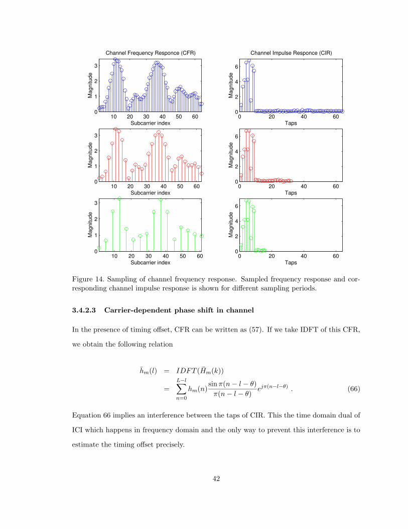
The errors on the frequency domain channel estimation, which can be modeled as white
noise, will effect the calculated CIR which in turn will effect the estimated parameters. Only
the taps where energy is concentrated will be used for CIR after IDFT is taken. Therefore,
for small sampling periods, i.e. small Sf , noise power will be spread over more taps while
CIR power is concentrated in the same number of taps always, increasing SNR. This can
be understood more clearly by analyzing Fig. 14. Sampled CFRs and corresponding CIRs
obtained by taking IDFT are shown in this figure. When no sampling is performed, noise
power is spread over 64 taps while signal power (CIR) is concentrated in the first 16 taps. As
more sampling is performed, the same noise power is now spread over less taps, increasing
MSE. This observation matches with the results shown in Fig. 15.
3.4.2.2 Constant phase shift in channel
A constant phase shift in the CFR will not change when IDFT operation is applied. Hence,
if there is a phase offset, Φ, in the CFR, the CIR calculated using the sampled version of
this channel will be
hm(l) = hm(l)ejΦ . (65)
This phase shift in the CIR has no significance since the statistics like RMS delay spread
and maximum excess delay depends only on the magnitude of CIR.
41
10 20 30 40 50 600
1
2
3
Subcarrier index
Mag
nitu
de
Channel Frequency Responce (CFR)
0 20 40 600
2
4
6
Channel Impulse Responce (CIR)
Taps
Mag
nitu
de
10 20 30 40 50 600
1
2
3
Subcarrier index
Mag
nitu
de
0 20 40 600
2
4
6
Taps
Mag
nitu
de
10 20 30 40 50 600
1
2
3
Subcarrier index
Mag
nitu
de
0 20 40 600
2
4
6
Taps
Mag
nitu
de
Figure 14. Sampling of channel frequency response. Sampled frequency response and cor-responding channel impulse response is shown for different sampling periods.
3.4.2.3 Carrier-dependent phase shift in channel
In the presence of timing offset, CFR can be written as (57). If we take IDFT of this CFR,
we obtain the following relation
hm(l) = IDFT (Hm(k))
=L−l∑
n=0
hm(n)sin π(n − l − θ)
π(n − l − θ)ejπ(n−l−θ) . (66)
Equation 66 implies an interference between the taps of CIR. This the time domain dual of
ICI which happens in frequency domain and the only way to prevent this interference is to
estimate the timing offset precisely.
42
0 5 10 15 20 250
0.2
0.4
0.6
0.8
1
1.2
1.4
Channel SNR (dB)
Mea
n sq
uare
d er
ror
Sf=1, Sim
Sf=1, Theo
Sf=2, Sim
Sf=2, Theo
Sf=4, Sim
Sf=4, Theo
Sf=5, Sim
Figure 15. Normalized mean squared error versus channel SNR for different sampling inter-vals. Simulation results and theoretical results are shown.
3.5 Performance results
Performance results of the proposed algorithms are obtained by simulating an OFDM system
with 64 subcarriers. Wireless channel is modeled with a 16-tap symbol-spaced CIR with
an exponentially decaying PDP. The channel taps are obtained by using a modified Jakes’
model [22]. Speed of the mobile is assumed to be 30 km/h.
Fig. 16 shows the difference between the frequency correlation estimates and ideal cor-
relation values for different RMS delay spreads. Ideal channel frequency correlation is
obtained by taking the Fourier transform of PDP. As can be seen, the correlation estimates
are very close to the ideal correlation values.
As described in previous sections, correlation estimate is used to find the coherence
bandwidth for a given correlation value of K. This is illustrated in Fig. 12. Notice that
43
2 4 6 8 10 12 14 16 18 200.1
0.2
0.3
0.4
0.5
0.6
0.7
0.8
0.9
1
Frequency ( x 1/TOFDM
Hz)
Cha
nnel
freq
uenc
y co
rrel
atio
n
IdealEstimated
τrms
=τ0
τrms
=2τ0
τrms
=3τ0
Figure 16. Comparison of the estimated frequency correlation with the ideal correlation fordifferent RMS delay spread values. 4000 OFDM symbols are averaged and mobile speedwas 30km/h.
as RMS delay spread increases, coherence bandwidth decreases. Three different coherence
bandwidth estimates that corresponds to three different RMS delay spread values are shown
in this figure for K = 0.9.
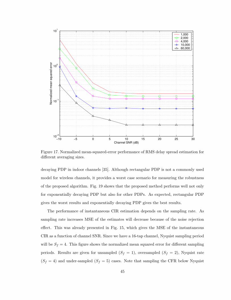
Fig. 17 shows the performance of the proposed RMS delay spread estimator as a function
of channel SNR. Normalized MSE performances are given for different number of OFDM
symbols that are used to obtain the CFC. As expected, the estimation error decreases as
the number of averages increases since calculated CFC is closer to the actual one.
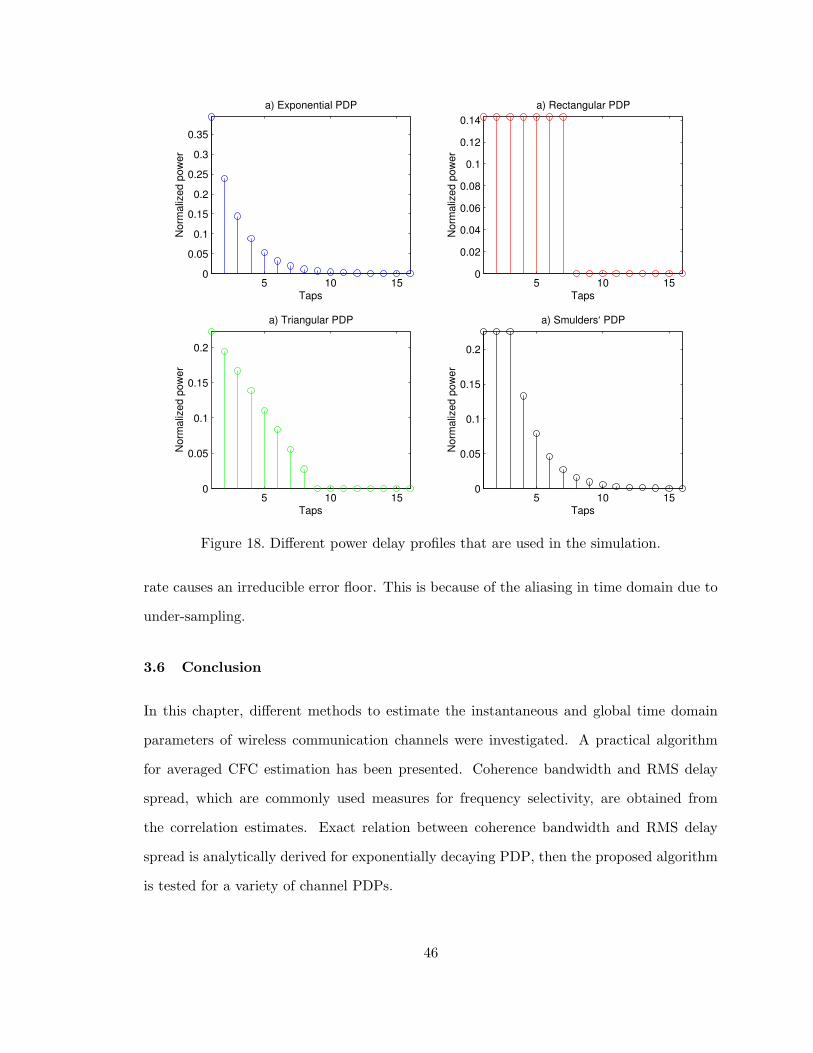
Figures 18 and 19 show PDPs used in the simulations and corresponding MSE per-
formances of the delay spread estimator respectively. Different PDPs are used in order
to test the robustness of the proposed method in different environments. Smulders’ PDP
is included as it has been considered by many authors as an alternative to exponentially
where a1, a2, . . . , aM are constants called the AR parameters, and v(n) is a white-noise
process.
Equation 84 implies that if we know the parameters, a1, a2, . . . , aM , then we can whiten
the signal u(n) by convolving it with the sequence of parameters am.
62
The relationship between the parameters of the model and the autocorrelation function
of u(n), rxx(l), is given by the Yule-Walker equations
rxx(l) =
∑Mk=1 akrxx(l − k) for n ≥ 1
∑Mk=1 akrxx(−k) + σ2
v for n = 0(85)
where σ2v = E{|v(n)|2}.
Therefore if we are know the input sequence u(n), we can obtain the autocorrelation
and we can solve for the model parameters, ak, by using Levinson-Durbin algorithm.
4.4.1.2 Estimation of noise spectrum and whitening
ICI samples of different carriers are correlated since the summation in (68) depends on the
same transmitted symbols, which makes ICI colored. Fig. 26 shows the Power Spectral
Density (PSD) of ICI sequence, which has low-pass characteristics. In Fig. 26, the spectral
power densities of ICI sequences whitened with AR filters of different model orders is also
given. As model order increases the spectrum becomes less colored, however this increases
the computational complexity.
We whiten the ICI signal since the receivers will perform much better in the presence
of white noise. Since ICI for each OFDM symbol depends on the instantaneous carrier
frequency offset or Doppler shift, we need to estimate the ICI samples for each OFDM
symbol independently. A two stage detection technique will be employed. In the first stage,
tentative symbol decisions will be performed using initially received signal. Then, these
initial estimates will be used to estimate the ICI present on the current OFDM symbol.
These estimates, then, will be used to find the AR model parameters and to whiten the
interference. After this process, the received signal with white noise will be used in a second
stage to provide symbol decisions.
Since we can not distinguish ICI from other impairments (e.g. additive noise, CCI, ACI,
etc.), we calculated ICI + other interferences and whitened this sum. Assuming we made
correct symbol decisions in the first stage and assuming perfect channel knowledge, we can
63
−1 −0.8 −0.6 −0.4 −0.2 0 0.2 0.4 0.6 0.8 1
x 107
−40
−35
−30
−25
−20
−15
−10
Frequency (Hz)
PS
D (d
B)
ICI signalAR 1AR 2AR 15
Figure 26. Power spectral density of the original and whitened versions of the ICI signalsfor different AR model orders.
find the total impairments by subtracting the re-modulated symbols from the impaired
received symbols.
We fit the spectrum of colored noise by an AR stochastic process of order M and
calculated the AR parameters. Having the AR filter coefficients, we can whiten the colored
noise by passing it through the AR filter. Although, filtering will whiten the colored signal,
it will effect the desired signal also. To recover the desired signal back, we can use M tap
Decision Feedback Equalizer (DFE), with M is equal to the order of the AR filter.
4.4.2 Performance results
The gain obtained using the proposed algorithm is proportional to the AR model order.
However, as the model order increases the computational complexity is also increasing.
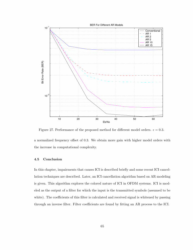
Fig. 27 shows the bit error rate for different AR model orders. This figure is obtained with
64
10 20 30 40 50 60
10−2
10−1BER For Different AR Models
Bit
Err
or R
ate
(BE
R)
Eb/No
ConventionalAR 1AR 2AR 5AR 10AR 15
Figure 27. Performance of the proposed method for different model orders. ε = 0.3.
a normalized frequency offset of 0.3. We obtain more gain with higher model orders with
the increase in computational complexity.
4.5 Conclusion
In this chapter, impairments that causes ICI is described briefly and some recent ICI cancel-
lation techniques are described. Later, an ICI cancellation algorithm based on AR modeling
is given. This algorithm explores the colored nature of ICI in OFDM systems. ICI is mod-
eled as the output of a filter for which the input is the transmitted symbols (assumed to be
white). The coefficients of this filter is calculated and received signal is whitened by passing
through an inverse filter. Filter coefficients are found by fitting an AR process to the ICI.
65
CHAPTER 5
ICI CANCELLATION BASED CHANNEL ESTIMATION
5.1 Introduction
Channel estimation is one of the most important elements of wireless receivers that em-
ploys coherent demodulation. For Orthogonal Frequency Division Multiplexing (OFDM)
based systems, channel estimation has been studied extensively. Approaches based on
Least Squares (LS), Minimum Mean-square Error (MMSE) [45], and Maximul Likelihood
(ML) [59] estimation are studied by exploiting the training sequences that are transmitted
along with the data. The previous channel estimation algorithms treat Inter-carrier Inter-
ference (ICI) as part of the additive white Gaussian noise and these algorithms perform
poorly when ICI is significant. Linear Minimum Mean-square Error (LMMSE) estimator is
analyzed in [46] to suppress the ICI due to mobility (Doppler spread). However, it is shown
that non-adaptive LMMSE estimator given in [46] is not capable of reducing ICI and the
design of an adaptive LMMSE is relatively difficult since both Doppler profile and noise
level need to be known. A channel estimation scheme which uses time-domain filtering to
mitigate the ICI effect of time-varying channel is proposed in [60].
This chapter presents a novel channel estimation method that eliminates ICI by jointly
finding the frequency offset and Channel Frequency Response (CFR). The proposed method
finds channel estimates by hypothesizing different frequency offsets and chooses the best
channel estimate using correlation properties of CFR. In the rest of this chapter, the pro-
posed algorithm will be described briefly and simulation results will be given.
66
5.2 System model
Time domain representation of OFDM signal is given is (3). This signal is cyclically ex-
tended to avoid Inter-symbol Interference (ISI) from previous symbol and transmitted.
At the receiver, the signal is received along with noise. After synchronization, down
sampling, and removal of cyclic prefix, the baseband model of the received frequency domain
samples can be written in matrix form as
y = SεpXh + z , (86)
where y is the vector of received symbols, X is a diagonal matrix with the transmitted
(training) symbols on its diagonal, h = [H(1) H(2) · · ·H(N)]T is the vector representing
the CFR to be estimated, and z is the additive white Gaussian noise vector with mean
zero and variance of σ2z . The N × N matrix, Sεp , is the interference (crosstalk) matrix
that represents the leakage between subcarriers, i.e. ICI. If there is no frequency offset, i.e.
εp = 0, Sεp becomes S0 = I, which implies no interference from neighboring subcarriers. If
ICI is assumed to be caused only by frequency offset, entries of Sεhcan be found using the
following formula [47]
Sεp(m, n) =sin π(m − n + εp)
N sin πN (m − n + εp)
ejπ(m−n+εp) , (87)
where εp is the present normalized carrier frequency offset (the ratio of the actual frequency
offset to the inter-subcarrier spacing).
5.3 Algorithm description
The interference matrix Sεp is not known to the receiver as it depends on the unknown
carrier frequency offset, εp. In this section, we will try to match to Sεp by Sεh, where εh is
the hypothesis for the true frequency offset.
67
The estimate of CFR is obtained by multiplying both sides of (86) with (SεhX)−1 as
(SεhX)−1
y = (SεhX)−1
SεpXh + (SεhX)−1
z
hεh= X−1Sεh
−1SεpXh + zεh. (88)
The inversion of the matrix SεhX is simple since the interference matrix Sεh
is unitary
and the data matrix X is diagonal. In this chapter, we assume that all of the sub-carriers are
used in training sequence i.e., no virtual carriers. This assumption ensures the invertibility
of training data matrix X.
Equation 88 will yield several channel estimates for different frequency offset hypothe-
ses. For the offset hypothesis, εh, which is closest to the actual frequency offset, εp, (88) will
yield the best estimate of the CFR. For choosing the best hypothesis, channel frequency
correlation is used as a decision criteria. In the rest of this section, properties of the interfer-
ence matrix will be described first. Then, the method for choosing the best hypothesis will
be explained followed by the description of the search algorithm to find the best hypothesis.
5.3.1 Properties of interference matrix
The following properties related to the interference matrix can be derived using (87).
1. SHS = I : Interference matrix is a unitary matrix. Therefore, the inverse of the
interference matrix can be calculated easily by taking the conjugate transpose since
S−1 = SH . Note that the superscript H represents conjugate transpose.
2. Sε1Sε2 = Sε1+ε2 : If two interference matrices corresponding to two different frequency
offsets are multiplied, another interference matrix corresponding to the sum can be
obtained. This property is exploited in the search algorithm.
3. S−ε = SHε : The interference matrix for a negative frequency offset can be obtained
from the interference matrix corresponding to a positive frequency offset with the
same magnitude by finding the complex transpose.
68
5.3.2 Channel frequency correlation for choosing the best hypothesis
The multiplication of two interference matrices in (88) can be written using the properties
of interference matrix as
S−1εh
Sεp = S−εhSεp = Sεp−εh
= Sεr , (89)
where εr is the difference between the actual frequency offset and frequency offset hypothesis,
i.e. residual frequency error.
Using (88) and (89), the estimate of the channel frequency response can be written as
Hεh(k) =
1
Xk
N∑
l=1
X(l)H(l)Sεr(k, l)
+1
Xk
N∑
l=1
z(l)Sεh(k, l) 1 ≤ k ≤ N . (90)
Using (90), the frequency correlation of the estimated channel for each OFDM symbol
can be calculated as
φhεh(∆) =
1
N − 2∆
N−∆∑
k=∆+1
{
Hεh(k)H∗
εh(k − ∆)
}
=1
N − 2∆
N−∆∑
k=∆+1
{
1
X(k)
N∑
l=1
X(l)H(l)Sεr(k, l)
· 1
X∗(k − ∆)
N∑
u=1
X∗(u)H∗(u)S∗εr
(k − ∆, u)
+1
X(k)
N∑
l=1
z(l)Sεh(k, l)
· 1
X∗(k − ∆)
N∑
u=1
z∗(u)Sεh(k − ∆, u)
}
. (91)
69
If we assume that the number of subcarriers, N , is large, (91) can be simplified as
φhεh(∆) =
φh(0) + σ2z
σ2s
∆ = 0
φh(∆)|Sεr(0)|2 ∆ 6= 0(92)
where |Sεr(0)| = sin (πεr)N sin (πεr/N) is the magnitude of the diagonal element of interference matrix
of residual frequency offset, Sεr and σ2s is the variance of the received signal. Note that as
the residual frequency offset increases, the value of |Sεr(0)| decreases, causing the correlation
to decrease.
As (92) implies, the correlation magnitude of the CFR depends on the residual fre-
quency offset. For a given CFR, channel frequency correlation becomes maximum when
the frequency offset hypothesis, εh, matches to the actual frequency offset. Therefore, the
correlation values can be used as a decision criteria for choosing the best hypothesis. For
choosing the best hypothesis among several hypotheses, this criteria is used in the search
algorithm
According to (92), all the lags of channel correlation can be used for obtaining the
best hypothesis. However, as ∆ increases channel correlation decreases, this degrades the
performance of the estimation since the ratio of useful signal power to the noise power
becomes smaller. Also, for large ∆ values, correlations are more noisy since less samples
are used to obtain these correlations. Moreover, increasing the number of lags increases the
computational complexity as more correlations need to be estimated. Therefore, selection
of the number of lags to be used is a design criteria and needs to be further investigated.
In our simulation, only the first correlation value, φhεh(1), is used. However, better
results can be obtained by effectively combining the information from other correlation
lags.
5.3.3 The search algorithm
Finding the frequency domain channel for all of the hypotheses and choosing the best hy-
pothesis require enormous computation. The interference matrices for each frequency offset
70
hypothesis should also be precomputed and stored in memory. However, these require-
ments can be relaxed by employing an optimum search algorithm. Instead of trying all
possible frequency offsets, the correct frequency offset is calculated by using a binary search
algorithm.
The magnitude of the correlation is estimated at the maximum and minimum expected
frequency offset values first. If the value at the minimum point is smaller, correct frequency
offset is expected to be at the bottom half of the initial interval. Therefore, maximum point
is moved to the point between the previous two points and minimum is not changed. If
maximum point is smaller, opposite operation is performed. In the second step the same
operation is repeated for the new interval. Then, this process is repeated for a predefined
number of iterations. Note that CFR needs to be obtained only for one more hypothesis
in each iteration after the first iteration. Therefore the total number of CFRs estimated is
total number of iterations plus one.
To calculate the CFR for a hypothesis, we do not need to have all the interference
matrices. If the interference matrices for εmax, εmax/2, εmax/4, εmax/8, . . . are calculated,
where εmax is the maximum expected frequency offset, the required interference matrices
can be found by using the second property of interference matrix. Moreover, CFR estimates
can be calculated without having all of the interference matrices. In (88), received symbols
are multiplied by S−1εh
and then multiplied with the diagonal matrix X−1. The result of
multiplication with S−1εh
can be stored and multiplied with S−1ε2 in the next step to obtain
the same result which would be obtained by multiplying S−1εh+ε2 .
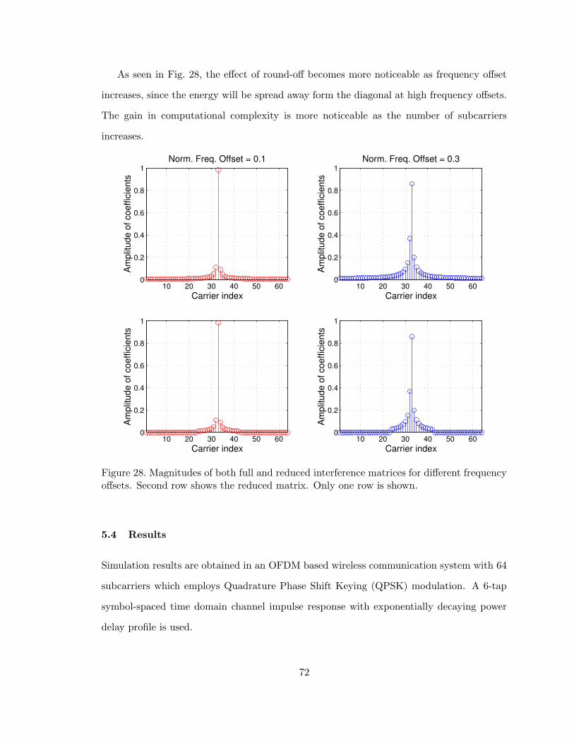
5.3.4 Reduced interference matrix
The interference matrix S is an N ×N matrix. However, most of the energy is concentrated
around the diagonal, i.e. interference is mostly due to neighboring subcarriers. The entries
away from the diagonal are set to zero in order to decrease the number of multiplications
and additions performed during the search algorithm. This will also decrease the memory
requirement. The amplitudes of the full and reduced interference matrices are shown in
Fig. 28 for normalized frequency offsets of 0.1 and 0.3.
71
As seen in Fig. 28, the effect of round-off becomes more noticeable as frequency offset
increases, since the energy will be spread away form the diagonal at high frequency offsets.
The gain in computational complexity is more noticeable as the number of subcarriers
increases.
10 20 30 40 50 600
0.2
0.4
0.6
0.8
1
Carrier index
Am
plitu
de o
f coe
ffici
ents
Norm. Freq. Offset = 0.3
10 20 30 40 50 600
0.2
0.4
0.6
0.8
1
Carrier index
Am
plitu
de o
f coe
ffici
ents
10 20 30 40 50 600
0.2
0.4
0.6
0.8
1
Carrier index
Am
plitu
de o
f coe
ffici
ents
Norm. Freq. Offset = 0.1
10 20 30 40 50 600
0.2
0.4
0.6
0.8
1
Carrier index
Am
plitu
de o
f coe
ffici
ents
Figure 28. Magnitudes of both full and reduced interference matrices for different frequencyoffsets. Second row shows the reduced matrix. Only one row is shown.
5.4 Results
Simulation results are obtained in an OFDM based wireless communication system with 64
subcarriers which employs Quadrature Phase Shift Keying (QPSK) modulation. A 6-tap
symbol-spaced time domain channel impulse response with exponentially decaying power
delay profile is used.
72
Number of iterations for the search algorithm was 8, which means that CFR is estimated
for 8 + 1 = 9 different frequency offset hypotheses to find the best CFR.
Fig. 29 shows the variance of the frequency offset estimator as a function of Signal-to-
noise Ratio (SNR). Results for full and reduced interference matrices are shown. Reduced
matrix is obtained using the 32 entries of full interference matrix, reducing computational
complexity by 50%. The Cramer-Rao bound [61]
CRB(ε) =1
2π2
3(SNR)−1
N(1 − 1/N2)(93)
is also provided for comparison. As can be seen from this figure, truncating the interference
matrix has little effect on the performance.
5 10 15 20 25 30 3510−7
10−6
10−5
10−4
10−3
SNR (dB)
Mea
n sq
uare
d er
ror
Full MatrixReduced MatrixCR Bound
Figure 29. Variance of the frequency offset estimator. Results obtained by using full andreduced interference matrices and Cramer-Rao lower bound is shown.
73
The frequency range in which the frequency offset is being searched is chosen adaptively
depending on the history of the estimated frequency offsets. If the variance of previous
frequency offset estimates is small, the range is decreased to increase the performance with
the same number of iterations; and if it is large the range is increased in order to be able
to track the variations of the frequency offset. Fig. 30 shows the correct and estimated
frequency offset values that are obtained by fixing the frequency offset range and changing
it adaptively. It can be seen from this figure that the algorithm converges to the correct
frequency offset and changing the range adaptively helps tracing the frequency offset.
0 20 40 60 80 100 120−0.2
0
0.2
0.4
0.6
0.8
1
1.2
OFDM frames
Nor
mal
ized
freq
uenc
y of
fset
Corect frequency offsetAdaptive offset rangeFixed offset range
Figure 30. Estimated and correct (normalized) frequency offset values at 10 dB. Results foradaptive and fixed initial frequency offset ranges are shown.
Mean-square error performances of the proposed and conventional LS estimators are
shown in Fig. 31 as a function of SNR, where a normalized frequency offset of 0.05 is used.
Obtained channel estimates can be further processed to decrease the mean-square error,
however this is out of the scope of this this study.
74
5 10 15 20 25 30 3510−3
10−2
10−1
100
SNR (dB)
Mea
n sq
uare
d er
ror
Least Squares MethodProposed Method
Figure 31. Mean-square error versus SNR for conventional LS and proposed CFR estimators.Normalized carrier frequency is 0.05.
5.5 Conclusion
A novel frequency-domain channel estimator which mitigates the effects of ICI by jointly
finding the frequency offset and CFR is described in this chapter. Unlike conventional
channel estimation techniques, where ICI is treated as part of the noise, the proposed
approach considers the effect of frequency offset in estimation of CFR. Methods to find the
best CFR effectively with low complexity is discussed. It is shown via computer simulations
that the proposed method is capable of reducing the effect of ICI on the frequency domain
channel estimation.
75
CHAPTER 6
CONCLUSION
The demand for high data rate wireless communication has been increasing dramatically
over the last decade. One way to transmit this high data rate information is to employ well-
known conventional single-carrier systems. Since the transmission bandwidth is much larger
than the coherence bandwidth of the channel, highly complex equalizers are needed at the
receiver for accurately recovering the transmitted information. Multi-carrier techniques can
solve this problem significantly if designed properly. Optimal and efficient design leads to
adaptive implementation of multi-carrier systems. Examples to adaptive implementation
methods in multi-carrier systems include adaptation of cyclic prefix length, sub-carrier
spacing etc. These techniques are often based on the channel statistics which need to be
estimated.
In this thesis, methods to estimate parameters for one of the most important statistics
of the channel which provide information about the frequency selectivity has been studied.
These parameters can be used to change the length of cyclic prefix adaptively depending
on the channel conditions. They can also be very useful for other transceiver adaptation
techniques.
Although multi-carrier systems handle the dispersion in time, they bring about other
problems like Inter-carrier Interference (ICI). In this thesis, ICI problem is studied for
improving the performance of both data detection and channel estimation at the receiver.
ICI problem is created to solve the problem with time dispersion, i.e., Inter-symbol
Interference (ISI). Depending on the application and the channel statistics, one problem
will be more significant than the other. For example for high data rate applications, ISI
appears to be more significant problem. On the other hand, for high mobility applications,
76
ICI is a more dominant impairment. For high data rate and high mobility applications,
the systems should be able to handle these interference sources efficiently, as they will
appear one way or another. Adaptive system design and adaptive interference cancellation
techniques, therefore, are very important to achieve this goal.
Current applications of Orthogonal Frequency Division Multiplexing (OFDM) do not
require high mobility. For next generation applications, however, it is crucial to have systems
that can tolerate high Doppler shifts caused by high mobile speeds. Current OFDM systems
assume that the channel is time-invariant over OFDM symbol. As mobility increases, this
assumption will not be valid anymore, and variations of the channel during the OFDM
symbol period will cause ICI as explained in Chapter 2. In the proposed channel estimation
method given in Chapter 5, only ICI due to frequency offset is considered. ICI due to time-
varying channel should be investigated further and effective channel estimation methods
that are immune to ICI due to mobility should be developed to have OFDM ready for high
mobility applications.
77
REFERENCES
[1] B. Saltzberg, “Performance of an efficient parallel data transmission system,” IEEETrans. Commun., vol. 15, no. 6, pp. 805–811, Dec. 1967.
[2] S. B. Weinstein and P. M. Ebert, “Data transmission by frequency-division multiplexingusing the discrete fourier transform,” IEEE Trans. Commun., vol. 19, no. 5, pp. 628–634, Oct. 1971.
[3] Radio broadcasting systems; Digital Audio Broadcasting (DAB) to mobile, portable andfixed receivers, ETSI – European Telecommunications Standards Institute Std. EN 300401, Rev. 1.3.3, May 2001.
[4] Digital Video Broadcasting (DVB); Framing structure, channel coding and modulationfor digital terrestrial television, ETSI – European Telecommunications Standards In-stitute Std. EN 300 744, Rev. 1.4.1, Jan. 2001.
[5] Asymmetric Digital Subscriber Line (ADSL), ANSI – American National StandardsInstitute Std. T1.413, 1995.
[6] Broadband Radio Access Networks (BRAN); HIPERLAN Type 2; Physical (PHY)layer, ETSI – European Telecommunications Standards Institute Std. TS 101 475,Rev. 1.3.1, Dec. 2001.
[7] Supplement to IEEE standard for information technology telecommunications and in-formation exchange between systems - local and metropolitan area networks - specificrequirements. Part 11: wireless LAN Medium Access Control (MAC) and PhysicalLayer (PHY) specifications: high-speed physical layer in the 5 GHz band, The Instituteof Electrical and Electronics Engineering, Inc. Std. IEEE 802.11a, Sept. 1999.
[8] Broadband Mobile Access Communication System (HiSWANa), ARIB – Association ofRadio Industries and Businesses Std. H14.11.27, Rev. 2.0, Nov. 2002.
[9] “IEEE 802.15 wpan high rate alternative PHY task group 3a (tg3a) website.” [Online].Available: http://www.ieee802.org/15/pub/TG3a.html
[10] M. Sternad, T. Ottosson, A. Ahlen, and A. Svensson, “Attaining both coverage andhigh spectral efficiency with adaptive OFDM downlinks,” in Proc. IEEE Veh. Technol.Conf., Orlando, FL, Oct. 2003.
[11] F. Sanzi and J. Speidel, “An adaptive two-dimensional channel estimator for wirelessOFDM with application to mobile DVB-T,” IEEE Trans. Broadcast., vol. 46, no. 2,pp. 128–133, June 2000.
78
[12] H. Arslan and T. Yucek, “Delay spread estimation for wireless communication sys-tems,” in Proc. IEEE Symposium on Computers and Commun., Antalya, TURKEY,June/July 2003, pp. 282–287.
[13] ——, “Estimation of frequency selectivity for OFDM based new generation wirelesscommunication systems,” in Proc. World Wireless Congress, San Francisco, CA, May2003.
[14] ——, “Frequency selectivity and delay spread estimation for adaptation of OFDMbased wireless communication systems,” EURASIP Journal on Applied Signal Pro-cessing, submitted for publication.
[15] K. Sathananthan and C. Tellambura, “Performance analysis of an OFDM system withcarrier frequency offset and phase noise,” in Proc. IEEE Veh. Technol. Conf., vol. 4,Atlantic City, NJ, Oct. 2001, pp. 2329–2332.
[16] H. Cheon and D. Hong, “Effect of channel estimation error in OFDM-based WLAN,”IEEE Commun. Lett., vol. 6, no. 5, pp. 190–192, May 2002.
[17] T. Yucek and H. Arslan, “ICI cancellation based channel estimation for OFDM sys-tems,” in Proc. IEEE Radio and Wireless Conf., Boston, MA, Aug. 2003, pp. 111–114.
[18] S. K. Mitra, Digital Signal Processing: A Computer-Based Approach, 2nd ed. NewYork, NY: McGraw-Hill, 2000.
[19] W. Henkel, G. Taubock, P. Odling, P. Borjesson, and N. Petersson, “The cyclic prefixof OFDM/DMT - an analysis,” in International Zurich Seminar on Broadband Com-munications. Access, Transmission, Networking., Zurich, Switzerland, Feb. 2002, p.1/3.
[20] F. Tufvesson, “Design of wireless communication systems – issues on synchronization,channel estimation and multi-carrier systems,” Ph.D. dissertation, Lund University,Aug. 2000.
[21] E. P. Lawrey, “Adaptive techniques for multiuser OFDM,” Ph.D. dissertation, JamesCook University, Dec. 2001.
[22] P. Dent, G. Bottomley, and T. Croft, “Jakes fading model revisited,” IEE Electron.Lett., vol. 29, no. 13, pp. 1162–1163, June 1993.
[23] P. H. Moose, “A technique for orthogonal frequency division multiplexing frequencyoffset correction,” IEEE Trans. Commun., vol. 42, no. 10, pp. 2908–2914, Oct. 1994.
[24] A. G. Armada, “Understanding the effects of phase noise in orthogonal frequencydivision multiplexing (OFDM),” IEEE Trans. Broadcast., vol. 47, no. 2, pp. 153–159,June 2002.
[25] T. May and H. Rohling, “Reducing the peak-to-average power ratio in OFDM ra-dio transmission systems,” in Proc. IEEE Veh. Technol. Conf., vol. 3, Ottawa, Ont.,Canada, May 1998, pp. 2474–2478.
79
[26] S. Muller and J. Huber, “A comparison of peak power reduction schemes for OFDM,”in Proc. IEEE Global Telecommunications Conf., vol. 1, Phoenix, AZ, USA, Nov. 1997,pp. 1–5.
[27] H. Ochiai and H. Imai, “On the distribution of the peak-to-average power ratio inOFDM signals,” IEEE Trans. Commun., vol. 49, no. 2, Feb. 2001.
[28] E. Lawrey and C. Kikkert, “Peak to average power ratio reduction of OFDM signalsusing peak reduction carriers,” in Signal Processing and Its Applications, 1999. ISSPA’99. Proceedings of the Fifth International Symposium on, vol. 2, Brisbane, Qld., Aus-tralia, Aug. 1999, pp. 737–740.
[29] J.-T. Chen, J. Liang, H.-S. Tsai, and Y.-K. Chen, “Joint MLSE receiver with dynamicchannel description,” IEEE J. Select. Areas Commun., vol. 16, pp. 1604–1615, Dec.1998.
[30] L. Husson and J.-C. Dany, “A new method for reducing the power consumption ofportable handsets in TDMA mobile systems: Conditional equalization,” IEEE Trans.Veh. Technol., vol. 48, pp. 1936–1945, Nov. 1999.
[31] H. Schober, F. Jondral, R. Stirling-Gallacher, and Z. Wang, “Adaptive channel es-timation for OFDM based high speed mobile communication systems,” in Proc. 3rdGeneration Wireless and Beyond Conf., San Francisco, CA, May/June 2001, pp. 392–397.
[32] M. Engels, Ed., Wireless OFDM systems: How to make them work?, ser. The Kluwerinternational series in engineering and computer sience. Kluwer Academic Publishers,May 2002.
[33] D. Harvatin and R. Ziemer, “Orthogonal frequency division multiplexing performancein delay and Doppler spread channels,” in Proc. IEEE Veh. Technol. Conf., vol. 3,no. 47, Phoenix, AZ, May 1997, pp. 1644–1647.
[34] K. Witrisal, Y.-H. Kim, and R. Prasad, “Rms delay spread estimation technique usingnon-coherent channel measurements,” IEE Electron. Lett., vol. 34, no. 20, pp. 1918–1919, Oct. 1998.
[35] ——, “A new method to measure parameters of frequency selective radio channel usingpower measurements,” IEEE Trans. Commun., vol. 49, pp. 1788–1800, Oct. 2001.
[36] K. Witrisal and A. Bohdanowicz, “Influence of noise on a novel rms delay spreadestimation method,” in Proc. IEEE Int. Symposium on Personal, Indoor and MobileRadio Commun., vol. 1, London, U.K., Sept. 2000, pp. 560–566.
[37] H. Schober and F. Jondral, “Delay spread estimation for OFDM based mobile com-munication systems,” in Proc. European Wireless Conf., Florence, Italy, Feb. 2002, pp.625–628.
[38] C. Athaudage and A. Jayalath, “Delay-spread estimation using cyclic-prefix in wirelessOFDM systems,” in Proc. IEEE Int. Conf. on Acoust., Speech, and Signal Processing,vol. 4, Apr. 2003, pp. 668–671.
80
[39] W. Jakes, Microwave Mobile Communications, 1st ed. 445 Hoes Lane, Piscataway,NJ: IEEE Press, 1993.
[40] B. H. Fleury, “An uncertainty relation for WSS process and its application to WSSUS,”IEEE Trans. Commun., vol. 44, pp. 1632–1634, Dec. 1996.
[41] P. Robertson and S. Kaiser, “The effect of Doppler spreads in OFDM(A) mobile radiosystems,” in Proc. IEEE Veh. Technol. Conf., vol. 1, Amsterdam, The Netherlands,Sept. 1999, pp. 329–333.
[42] M. Russell and G. L. Stuber, “Interchannel interference analysis of OFDM in a mobileenvironment,” in Proc. IEEE Veh. Technol. Conf., vol. 2, Chicago, IL, July 1995, pp.820–824.
[43] L. Hazy and M. El-Tanany, “Synchronization of OFDM systems over frequency selec-tive fading channels,” in Proc. IEEE Veh. Technol. Conf., vol. 3, no. 47, Phoenix, AZ,May 1997, pp. 2094–2098.
[44] D. Matic, T. A. Coenen, F. C. Schoute, and R. Prasad, “OFDM timing synchronization:Possibilities and limits to the usage of the cyclic prefix for maximum likelihood estima-tion,” in Proc. IEEE Veh. Technol. Conf., vol. 2, no. 50, Amsterdam, The Netherlands,Sept. 1999, pp. 668–672.
[45] J.-J. van de Beek, O. Edfors, M. Sandell, S. Wilson, and P. Borjesson, “On channelestimation in OFDM systems,” in Proc. IEEE Veh. Technol. Conf., vol. 2, Chicago,IL, July 1995, pp. 815–819.
[46] A. Hutter, R. Hasholzner, and J. Hammerschmidt, “Channel estimation for mobileOFDM systems,” in Proc. IEEE Veh. Technol. Conf., vol. 1, Amsterdam, The Nether-lands, Sept. 1999, pp. 305–309.
[47] J. Armstrong, “Analysis of new and existing methods of reducing intercarrier interfer-ence due to carrier frequency offset in OFDM,” IEEE Trans. Commun., vol. 47, no. 3,pp. 365–369, Mar. 1999.
[48] J. Ahn and H. S. Lee, “Frequency domain equalization of OFDM signals over frequencynonselective rayleigh fading channels,” IEE Electron. Lett., vol. 29, no. 16, pp. 1476–1477, Aug. 1993.
[49] S. Chang and E. J. Powers, “Cancellation of inter-carrier interference in OFDM systemsusing a nonlinear adapive filter,” in Proc. IEEE Int. Conf. Commun., vol. 2, NewOrleans, LA, 2000, pp. 1039–1043.
[50] C. Muschallik, “Improving an OFDM reception using an adaptive Nyquist windowing,”IEEE Trans. Consumer Electron., vol. 42, no. 3, pp. 259–269, Aug. 1996.
[51] S. H. Muller-Weinfurtner, “Optimum Nyquist windowing in OFDM receivers,” IEEETrans. Commun., vol. 49, no. 3, pp. 417–420, Mar. 2001.
[52] K. Sathananthan and C. Tellambura, “Reducing intercarrier interference in OFDMsystems by partial transmit sequence and selected mapping,” in Proc. Int. Symposiumon DSP for Commun. Syst., Manly-Sydney, Australia, Jan. 2002, pp. 234–238.
81
[53] ——, “Novel adaptive modulation scheme to reduce both PAR and ICI of and OFDMsignal,” in Proc. Int. Symposium on DSP for Commun. Syst., Manly-Sydney, Australia,Jan. 2002, pp. 229–233.
[54] Y. Zhao, J.-D. Leclercq, and S.-G. Haggman, “Intercarrier interference compression inOFDM communications systems by using correlative coding,” IEEE Commun. Lett.,vol. 2, no. 8, pp. 214–216, Aug. 1998.
[55] Y. Zhao and S.-G. Haggman, “Intercarrier interference self-cancellation scheme forOFDM mobile communications systems,” IEEE Trans. Commun., vol. 49, no. 7, pp.1185–1191, July 2001.
[56] J. Armstrong, P. M. Grant, and G. Povey, “Polynomial cancellation coding of OFDM toreduce intercarrier interference due to Doppler spread,” in Proc. IEEE Global Telecom-munications Conf., vol. 5, Sydney, NSW, Australia, Nov. 1998, pp. 2771–2776.
[57] K. Sathananthan and C. Tellambura, “New ICI reduction schemes for OFDM systems,”Proc. IEEE Veh. Technol. Conf., vol. 2, no. 54, pp. 834–838, 2001.
[58] K. Sathananthan and R. Rajatheva, “Analysis of OFDM in the presence of frequencyoffset and a method to reduce performance degradation,” Proc. IEEE Global Telecom-munications Conf., vol. 1, pp. 2078–2079, 2000.
[59] P. Chen and H. Kobayashi, “Maximum likelihood channel estimation and signal de-tection for OFDM systems,” in Proc. IEEE Int. Conf. Commun., vol. 3, 2002, pp.1640–1645.
[60] A. Stamoulis, S. Diggavi, and N. Al-Dhahir, “Estimation of fast fading channels inOFDM,” in Proc. IEEE Wireless Commun. and Networking Conf., vol. 1, Orlando,FL, Mar. 2002, pp. 465–470.
[61] M. Morelli and U. Mengali, “An improved frequency offset estimator for OFDM appli-cations,” IEEE Commun. Lett., vol. 3, no. 3, pp. 75–77, Mar. 1999.