Self-similar asymptotics in evolution equations Grzegorz Karch Instytut Matematyczny, Uniwersytet Wroc lawski, pl. Grunwaldzki 2/4, 50-384 Wroclaw, Poland [email protected]http://www.math.uni.wroc.pl/∼karch Notes based on the series of lectures presented by the author in Faculty of Mathematics, Informatics and Mechanics of University of Warsaw in March– May, 2011. Abstract. A function is called a self-similar solution of an evolution equation if its value at a given time t 0 (e.g. at t 0 = 1 ) it sufficient to calculate this function for all other values of time t> 0 via so-called self-similar transformation. Self-similar solutions have always played in important role in the study of properties of other solutions to linear and nonlinear evolution equations. Very often, one can find explicit self-similar solutions which describe typical properties of other solutions. For example, the Gauss-Weierstrass kernel G(x, t) = (4πt) -n/2 e -|x| 2 /(4t) is the most famous solution of the heat equation u t =Δu. This explicit solution appears in the asymptotic expansions as t →∞ of other solutions to the initial value problem for the heat equation. In this series of lecture, participants will learn methods how to find for self-similar solutions of different nonlinear problem and how to use them to understand properties of other solutions.
Transcript
Self-similar asymptoticsin evolution equations
Grzegorz Karch
Instytut Matematyczny, Uniwersytet Wroc lawski,pl. Grunwaldzki 2/4, 50-384 Wroclaw, Poland
Notes based on the series of lectures presented by the author in Faculty ofMathematics, Informatics and Mechanics of University of Warsaw in March–May, 2011.
Abstract. A function is called a self-similar solution of an evolution equation if itsvalue at a given time t0 (e.g. at t0 = 1 ) it sufficient to calculate this function for allother values of time t > 0 via so-called self-similar transformation. Self-similar solutionshave always played in important role in the study of properties of other solutions to linearand nonlinear evolution equations. Very often, one can find explicit self-similar solutionswhich describe typical properties of other solutions. For example, the Gauss-Weierstrasskernel
G(x, t) = (4πt)−n/2e−|x|2/(4t)
is the most famous solution of the heat equation ut = ∆u. This explicit solution appearsin the asymptotic expansions as t→∞ of other solutions to the initial value problem forthe heat equation.
In this series of lecture, participants will learn methods how to find for self-similarsolutions of different nonlinear problem and how to use them to understand properties ofother solutions.
First, we consider the Cauchy problem for the heat equation
ut(x, t) = ∆u(x, t) for x ∈ Rn and t > 0 (1.1.1)
u(x, 0) = u0(x). (1.1.2)
A solution of the initial value problem (1.1.1)-(1.1.2) is represented by
u(x, t) =
∫
RnG(x− y, t)u0(y) dy for x ∈ Rn and t > 0, (1.1.3)
with the Gauss-Weierstrass kernel
G(x, t) =1
(4πt)n/2exp
(−|x|
2
4t
)for x ∈ Rn and t > 0. (1.1.4)
In these lecture notes,
for x ∈ Rn, we have always denoted |x| =√x21 + ...+ x2n.
The following theorem gathers typical properties of the solution u = u(x, t) defined in(1.1.3).
Theorem 1.1.1. Assume that u0 ∈ L1(Rn) and define u = u(x, t) by (1.1.3). Then
1. u ∈ C∞(Rn × (0,∞)),
2. u satisfies equation (1.1.1) for all x ∈ Rn and t > 0,
3. ‖u(·, t)− u0(·)‖1 → 0 when t→ 0,
4. ‖u(·, t)‖1 ≤ ‖u0(·)‖1 for all t ≥ 0.
This is the unique solution of problem (1.1.1)-(1.1.2) satisfying these properties.
The proof of this theorem can be found in the Evans book [8, Ch. 2.3].
1
21.1 Asymptotic Behavior of Solutions Near Time Infinity 5
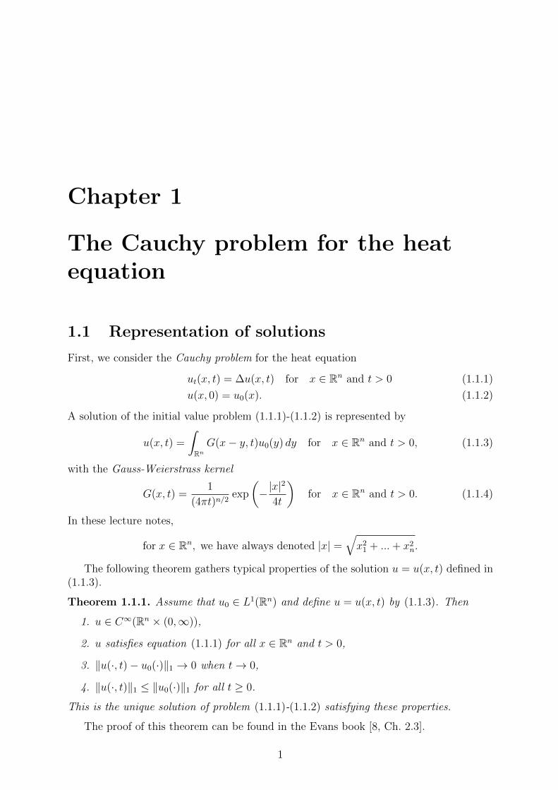
Figure 1.1. A few examples of the graph of Gt(x) as a function of x for n = 1.
or
u(x1, . . . , xn, t) =
∫ ∞
−∞· · ·∫ ∞
−∞Gt(x1 − y1, x2 − y2, . . . , xn − yn, t)
· f(y1, . . . , yn) dy1dy2 · · ·dyn
using the Gauss kernel
Gt(x) =1
(4πt)n/2exp
(−|x|2
4t
), x ∈ Rn, t > 0,
if the absolute value |f(x)| of the function f(x) does not grow too much atspace infinity. See figure 1.1.
Throughout this book, Gt denotes the Gauss kernel and exp z denotes theexponential function ez, where e is the base of the natural logarithm. Forx ∈ Rn, |x| denotes the Euclidean norm (x2
1 + x22 + · · · + x2
n)1/2 of x. Thefunction u of (1.3) is differentiable to any order with respect to x1, x2, . . . , xn
and t > 0, satisfies the heat equation (1.1) (See Exercise 1.1 (i) and 7.2 and§4.1.6), and satisfies (1.2) in the sense of limt→0 u(x, t) = f(x) (see §4.2) if,for example, f is continuous and f is equal to zero outside a large ball in Rn.We denote the set of such functions f by C0(Rn). See Figure 1.2. In Chapter 1,unless otherwise mentioned we assume that the initial data f is in C0(Rn),so that the solution u of (1.1), (1.2) is represented by (1.3). Although it isimportant to examine whether there exist other solutions satisfying (1.1),(1.2), we do not consider such a problem in this section. This is postponed to§4.4. When t → ∞ (i.e., t goes to infinity), to what function of x does u(x, t)
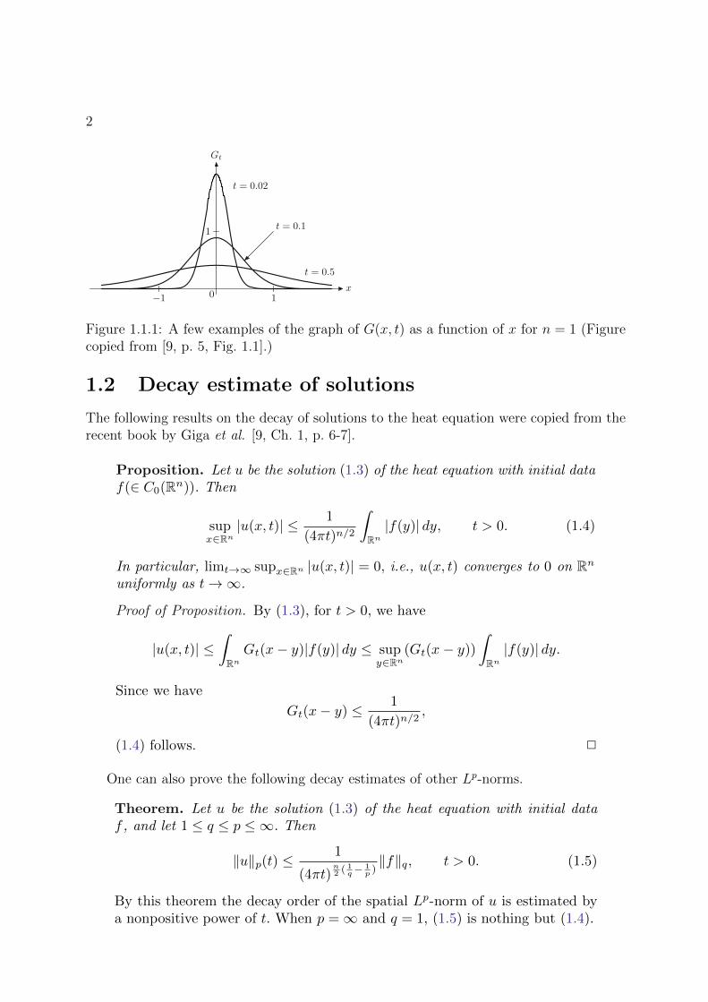
Figure 1.1.1: A few examples of the graph of G(x, t) as a function of x for n = 1 (Figurecopied from [9, p. 5, Fig. 1.1].)
1.2 Decay estimate of solutions
The following results on the decay of solutions to the heat equation were copied from therecent book by Giga et al. [9, Ch. 1, p. 6-7].
6 1 Behavior Near Time Infinity of Solutions of the Heat Equation
Figure 1.2. An example of the graph of f ∈ C0(R).
tend? We guess that u(x, t) tends to zero as t → ∞, since f is in C0(Rn)and there is no heat source. In the following, we prove that this observationis correct.
In this chapter unless otherwise specified, f belongs to C0(Rn), since thenthe integral of f can be regarded as an integral of a continuous functionon a sufficiently large ball, which is finite, so that it is easy to handle (seeExercise 1.1 (ii)). Of course, we may consider more general f . Inequalities in§1.1.1–§1.1.3 are also valid if the integral is well defined. For example, we mayconsider f as a continuous function such that the Riemann integral on theright-hand side of the inequality is finite, or more generally we may consider aLebesgue measurable function f with finite Lebesgue integral. In both cases,the inequalities in §1.1.1–§1.1.3 are valid. Here, to check the differentiabilityunder the integral is a good exercise in analysis, but we do not check it inthis chapter. Instead, see §4.1.4, §4.1.6, §7.2.1 and exercises at the end ofChapter 7.
1.1.1 Decay Estimate of Solutions
Proposition. Let u be the solution (1.3) of the heat equation with initial dataf(∈ C0(Rn)). Then
supx∈Rn
|u(x, t)| ≤ 1
(4πt)n/2
∫
Rn
|f(y)| dy, t > 0. (1.4)
In particular, limt→∞ supx∈Rn |u(x, t)| = 0, i.e., u(x, t) converges to 0 on Rn
uniformly as t → ∞.
1.1 Asymptotic Behavior of Solutions Near Time Infinity 7
Before giving the proof, we recall the notation sup, which represents thesupremum of a set. For any subset A of R, the real numberM that satisfies thefollowing two conditions is called the supremum of the set A, and is denotedby supA (if A is bounded from above, the existence of such a number Mfollows from the definition of the real numbers):
(i) We have a ≤ M for any element a of A (i.e., a ∈ A). (Such an M is calledan upper bound of the set A.)
(ii) For any M ′ less than M (i.e., M ′ < M), there exists an element a′ of Asuch that a′ > M ′.
In other words, M is the minimal upper bound of A. For a set A with noupper bound we set supA = ∞, and for the empty set A we set supA = −∞.If A is the image of a real-valued function h defined on a set U , instead ofwriting supA as suph(x) : x ∈ U we may write
supx∈U
h(x) or simply supUh.
Its value is called the supremum of the function h in U . If there exists x0 ∈ Usatisfying
supx∈U
h(x) = h(x0),
supU h is called the maximum of h in U and is denoted by maxU h.In general such an x0 does not always exist, and even if it exists, showing its
existence may not be easy. On the other hand, the supremum is always definedfor any real-valued function, which makes it a convenient notion. If supU |h|is finite, h is said to be bounded in U .
Similarly, the infimum infU h of a function h on U is defined by
infx∈U
h(x) = − supx∈U
(−h(x)).
We sometimes write the range of the independent variables of a function hdirectly under “sup” or “inf” as in §1.3.3.
Proof of Proposition. By (1.3), for t > 0, we have
|u(x, t)| ≤∫
Rn
Gt(x− y)|f(y)| dy ≤ supy∈Rn
(Gt(x − y))
∫
Rn
|f(y)| dy.
Since we have
Gt(x− y) ≤ 1
(4πt)n/2,
(1.4) follows.
By this result we observe that u converges to 0 uniformly with order atleast t−n/2 as t → ∞. We next ask whether the space integral of |u| or its
One can also prove the following decay estimates of other Lp-norms.
8 1 Behavior Near Time Infinity of Solutions of the Heat Equation
power also decays. For this purpose we first define the Lp-norm and L∞-normof continuous functions f on Rn as
‖f‖p =
(∫
Rn
|f(y)|p dy)1/p
, 1 ≤ p < ∞ (p a constant),
‖f‖∞ = supy∈Rn
|f(y)|.
For simplicity, ‖f‖∞ denotes ‖f‖p with p = ∞. (This convention is natural bythe fact of Exercise 2.3.) Although ∞ and −∞ are not real numbers, we regard∞, −∞ as symbols that satisfy −∞ < a < ∞ for any real number a so thatwe are able to handle various inequalities in a synthetic way. Moreover, we usethe convention 1
∞ = 0, a + ∞ = ∞, since it is useful to shorten statements.For function u(x, t) with variable (x, t) ∈ Rn × (0,∞), ‖u‖p(t) denotes theLp-norm of u(x, t) as a function of x, i.e.,
‖u‖p(t) =
⎧⎪⎨⎪⎩
(∫
Rn
|u(x, t)|p dx)1/p
, 1 ≤ p < ∞, t > 0,
supx∈Rn |u(x, t)|, p = ∞, t > 0.
A more general estimate than in §1.1.1 holds.
1.1.2 Lp-Lq Estimates
Theorem. Let u be the solution (1.3) of the heat equation with initial dataf , and let 1 ≤ q ≤ p ≤ ∞. Then
‖u‖p(t) ≤ 1
(4πt)n2 ( 1
q − 1p )
‖f‖q, t > 0. (1.5)
By this theorem the decay order of the spatial Lp-norm of u is estimated bya nonpositive power of t. When p = ∞ and q = 1, (1.5) is nothing but (1.4).
Although the proof of this theorem is more complicated than that of (1.4),it can be proved easily using the Young inequality for convolutions (see §4.1.2).
We have studied the decay of the value of u. We ask whether the derivativesof u decay to 0 as t → ∞.
1.1.3 Derivative Lp-Lq Estimates
Theorem. Let u be the solution (1.3) of the heat equation with initial dataf . For 1 ≤ q ≤ p ≤ ∞ there exists a constant C = C(p, q, n) depending onlyon p, q, n such that
∥∥∥∥∂u
∂xj
∥∥∥∥p
(t) ≤ C
tn2 ( 1
q − 1p )+ 1
2
‖f‖q, j = 1, . . . , n, t > 0, (1.6)
3
Although the proof of this theorem is more complicated than that of (1.4), it can beproved easily using the Young inequality for convolutions.
Now, we recall a results on the decay of derivatives of a solution to problem (1.1.1)-(1.1.2), cf. [9, Ch. 1, p. 8-10].
8 1 Behavior Near Time Infinity of Solutions of the Heat Equation
power also decays. For this purpose we first define the Lp-norm and L∞-normof continuous functions f on Rn as
‖f‖p =
(∫
Rn
|f(y)|p dy)1/p
, 1 ≤ p < ∞ (p a constant),
‖f‖∞ = supy∈Rn
|f(y)|.
For simplicity, ‖f‖∞ denotes ‖f‖p with p = ∞. (This convention is natural bythe fact of Exercise 2.3.) Although ∞ and −∞ are not real numbers, we regard∞, −∞ as symbols that satisfy −∞ < a < ∞ for any real number a so thatwe are able to handle various inequalities in a synthetic way. Moreover, we usethe convention 1
∞ = 0, a + ∞ = ∞, since it is useful to shorten statements.For function u(x, t) with variable (x, t) ∈ Rn × (0,∞), ‖u‖p(t) denotes theLp-norm of u(x, t) as a function of x, i.e.,
‖u‖p(t) =
⎧⎪⎨⎪⎩
(∫
Rn
|u(x, t)|p dx)1/p
, 1 ≤ p < ∞, t > 0,
supx∈Rn |u(x, t)|, p = ∞, t > 0.
A more general estimate than in §1.1.1 holds.
1.1.2 Lp-Lq Estimates
Theorem. Let u be the solution (1.3) of the heat equation with initial dataf , and let 1 ≤ q ≤ p ≤ ∞. Then
‖u‖p(t) ≤ 1
(4πt)n2 ( 1
q − 1p )
‖f‖q, t > 0. (1.5)
By this theorem the decay order of the spatial Lp-norm of u is estimated bya nonpositive power of t. When p = ∞ and q = 1, (1.5) is nothing but (1.4).
Although the proof of this theorem is more complicated than that of (1.4),it can be proved easily using the Young inequality for convolutions (see §4.1.2).
We have studied the decay of the value of u. We ask whether the derivativesof u decay to 0 as t → ∞.
1.1.3 Derivative Lp-Lq Estimates
Theorem. Let u be the solution (1.3) of the heat equation with initial dataf . For 1 ≤ q ≤ p ≤ ∞ there exists a constant C = C(p, q, n) depending onlyon p, q, n such that
∥∥∥∥∂u
∂xj
∥∥∥∥p
(t) ≤ C
tn2 ( 1
q − 1p )+ 1
2
‖f‖q, j = 1, . . . , n, t > 0, (1.6)
1.1 Asymptotic Behavior of Solutions Near Time Infinity 9
∥∥∥∥∂u
∂t
∥∥∥∥p
(t) ≤ C
tn2 ( 1
q − 1p )+1
‖f‖q, t > 0. (1.7)
Moreover, for higher derivatives, there exists a constant C = C(p, q, n, k, α)such that
‖∂kt ∂
αx u‖p(t) ≤ C
tn2 ( 1
q − 1p )+k+ |α|
2
‖f‖q, t > 0. (1.8)
(Here k is a natural number or 0 and α is a multi-index (α1, . . . , αn); αi
(1 ≤ i ≤ n) is a natural number or 0. We use the convention
∂αx = ∂α1
x1∂α2
x2· · ·∂αn
xn, ∂xi =
∂
∂xi, ∂t =
∂
∂t,
|α| = α1 + · · · + αn,
∂0xiu = u, ∂0
t u = u.
In other words, |α| is the order of the derivative ∂αx in the spatial direction.)
We remark that one can choose the constants C in (1.6)–(1.8) independentof p and q.
By (1.6), (1.7), and (1.8), we observe that the power of t increases by 1/2by differentiating once in the spatial variables, and that it increases by 1 bydifferentiating in the time variable. Since the proof of ((1.8) for general cases issomewhat time-consuming, we shall prove (1.6) only when p = ∞ and q = 1,and leave the remaining proof to the reader. (See §4.1.2 and Exercise 4.3.)
Proof of (1.6) (In the case of p = ∞, q = 1). Differentiating (1.3) under theintegral, we have
∂xju(x, t) =
∫
Rn
(∂xjGt)(x− y)f(y) dy.
The symbol (∂xjGt)(x − y) is the quantity obtained by differentiating Gt(x)in xj and evaluating at x− y. A calculation shows that
∂xjGt(x) =1
(4πt)n/2
(−2xj
4t
)exp
(−|x|2
4t
).
The power of t seems to increase not by 1/2 but by 1. However, setting z =|x|/(2t1/2), we have
∣∣∣∣xj
2texp
(−|x|2
4t
)∣∣∣∣ ≤ 1
t12
z exp(−z2).
Fortunately, z exp(−z2) is a bounded function in z ≥ 0. In fact, z exp(−z2)attains its maximum C1 = 1/
√2e at z = 1/
√2. (See Exercise 1.2.) We obtain
4
1.1 Asymptotic Behavior of Solutions Near Time Infinity 9
∥∥∥∥∂u
∂t
∥∥∥∥p
(t) ≤ C
tn2 ( 1
q − 1p )+1
‖f‖q, t > 0. (1.7)
Moreover, for higher derivatives, there exists a constant C = C(p, q, n, k, α)such that
‖∂kt ∂
αx u‖p(t) ≤ C
tn2 ( 1
q − 1p )+k+ |α|
2
‖f‖q, t > 0. (1.8)
(Here k is a natural number or 0 and α is a multi-index (α1, . . . , αn); αi
(1 ≤ i ≤ n) is a natural number or 0. We use the convention
∂αx = ∂α1
x1∂α2
x2· · ·∂αn
xn, ∂xi =
∂
∂xi, ∂t =
∂
∂t,
|α| = α1 + · · · + αn,
∂0xiu = u, ∂0
t u = u.
In other words, |α| is the order of the derivative ∂αx in the spatial direction.)
We remark that one can choose the constants C in (1.6)–(1.8) independentof p and q.
By (1.6), (1.7), and (1.8), we observe that the power of t increases by 1/2by differentiating once in the spatial variables, and that it increases by 1 bydifferentiating in the time variable. Since the proof of ((1.8) for general cases issomewhat time-consuming, we shall prove (1.6) only when p = ∞ and q = 1,and leave the remaining proof to the reader. (See §4.1.2 and Exercise 4.3.)
Proof of (1.6) (In the case of p = ∞, q = 1). Differentiating (1.3) under theintegral, we have
∂xju(x, t) =
∫
Rn
(∂xjGt)(x− y)f(y) dy.
The symbol (∂xjGt)(x − y) is the quantity obtained by differentiating Gt(x)in xj and evaluating at x− y. A calculation shows that
∂xjGt(x) =1
(4πt)n/2
(−2xj
4t
)exp
(−|x|2
4t
).
The power of t seems to increase not by 1/2 but by 1. However, setting z =|x|/(2t1/2), we have
∣∣∣∣xj
2texp
(−|x|2
4t
)∣∣∣∣ ≤ 1
t12
z exp(−z2).
Fortunately, z exp(−z2) is a bounded function in z ≥ 0. In fact, z exp(−z2)attains its maximum C1 = 1/
√2e at z = 1/
√2. (See Exercise 1.2.) We obtain
10 1 Behavior Near Time Infinity of Solutions of the Heat Equation
‖∂xjGt‖∞ ≤ 1
(4πt)n2
C1
t12
.
Similarly as in the proof of (1.4), we have
∥∥∥∥∂u
∂xj
∥∥∥∥∞
≤ ‖∂xjGt‖∞
∫
Rn
|f(y)| dy ≤ C
tn2 + 1
2
‖f‖1, C = C11
(4π)n2,
which proves (1.6).
We call the estimate in §1.1.1 a decay estimate by focusing at the behaviorfor large t; however, the estimate also shows a decrease in smoothness of u ast tends to 0. For this reason, in §1.1.2–§1.1.3 we call the estimate not a decayestimate but an Lp-Lq-estimate.
In the above we have observed decay orders of various norms for thesolution of the initial value problem of the heat equation (1.1) with (1.2).How does u(x, t) converges to 0 as t tends to infinity? We already know thatthe solution u decays as ‖u‖∞ ≤ (4πt)−n/2‖f‖1 by (1.4). So, if we can find asimple well-known (nonzero) function v such that the L∞-norm ‖u− v‖∞(t)goes to 0 faster than t−n/2 as t → ∞, then we may say that u behaves likev for large t. In this situation v is called a leading term of the decay of u.What function is the leading term of the decay of the solution of the heatequation (1.1) with (1.2)? We would like to choose the function v as simple aspossible. The next result states that we may choose v as a constant multipleof the Gauss kernel.
1.1.4 Theorem on Asymptotic Behavior Near Time Infinity
Theorem. Let u be the solution (1.3) of the heat equation with initial dataf ∈ C0(Rn). Let m =
∫Rn f(y) dy. Then
limt→∞
tn/2‖u−mg‖∞(t) = 0, (1.9)
where g(x, t) = Gt(x) is the Gauss kernel.
This theorem shows that u has a similar behavior as mg to that of t → ∞when m = 0. Therefore (1.9) is often called an asymptotic formula, and wewrite
u ∼ mg (t → ∞).
This notation is good for intuitive understanding of the behavior of u; however,for a rigorous expression we need a formula like (1.9). Whenm = 0, (1.9) showsthat ‖u‖∞(t) goes to zero faster than t−n/2. In this case (1.9) does not give aleading term. We now prove the asymptotic formula (1.9).
1.3 Weak form of the initial value problem for the
heat equation
The following part is copied from [9, Ch. 1.4.2, p. 29-30]. Notice that, below, C∞0 (Rn ×[0,∞)) denotes the set of all functions from C∞(Rn × [0,∞)) with compact supports inRn × [0,∞). During lectures, such a set is denoted by C∞c (Rn × [0,∞))
5
1.4 Characterization of Limit Functions 29
This proposition is easily proved in a similar way as it is proved that u(x, t)defined by (1.3) converges to f(x) as t → 0, and we shall prove it in §4.2.5.In other words, fk converges to the m multiple of the Dirac δ distribution(δ measure) in the sense of measures (or distributions). The Dirac δ distri-bution can be regarded as the map that evaluates a continuous function atx = 0, i.e.,
δ : f → f(0)
for f ∈ C(Rn). When the initial data is not a function as in this case, how dowe interpret the initial condition?
1.4.2 Weak Form of the Initial Value Problem for the HeatEquation
Multiplying the heat equation ∂tu − Δu = 0 by ϕ ∈ C∞0 (Rn × [0,∞)), and
then integrating on Rn × (0,∞), we obtain
0 =
∫ ∞
0
∫
Rn
ϕ(∂tu−Δu) dx dt.
Using integration by parts (§4.5.3), for u ∈ C∞(Rn × [0,∞)) we have∫ ∞
0
ϕ∂tu dt = [ϕ(x, t)u(x, t)]∞t=0 −∫ ∞
0
u∂tϕdt
= −ϕ(x, 0)u(x, 0) −∫ ∞
0
u∂tϕdt,
∫
Rn
ϕΔudx = −∫
Rn
〈∇ϕ,∇u〉 dx =
∫
Rn
(Δϕ)u dx,
which yields1
0 = −∫
Rn
ϕ(x, 0)u(x, 0) dx −∫ ∞
0
∫
Rn
(∂tϕ+Δϕ)u dx dt. (1.16)
We do not carry out the justification of commutation of integrals in thischapter; in fact, the last equality is justified by Fubini’s theorem in §7.2.2.Of course, for u ∈ C∞(Rn × [0,∞)) it is sufficient to consider the Riemannintegral. Here, by definition, ϕ is zero for large t and for large |x|; however,we note that ϕ(x, 0) may not be identically zero (but belongs to C∞
0 (Rn)).Conversely, if u is smooth in Rn × (0,∞) and continuous in Rn × [0,∞)(i.e., u ∈ C∞(Rn × (0,∞)) ∩ C0(Rn × [0,∞)), and (1.16) holds for any ϕ ∈C∞
0 (Rn × [0,∞)), then u is a solution of the heat equation with initial datau(x, 0) (Exercise 1.8). Thus, we define weak solutions of the heat equation asfollows.1 The equation (1.16) also holds if u is continuous in Rn × [0, ∞) and smooth in
Rn × (0, ∞). In this case, we do not assume the continuity of ∂tu at t = 0; hence∫∞0
ϕ∂tu dt is not necessarily finite. So, we replace the time interval of integration(0, ∞) to (ε, ∞) (ε > 0) and integrate by parts then we obtain (1.16) by lettingε → 0.
30 1 Behavior Near Time Infinity of Solutions of the Heat Equation
1.4.3 Weak Solutions for the Initial Value Problem
Definition. Assume that u is locally integrable in Rn × [0,∞).
(i) Assume that f is locally integrable in Rn. A function u is called a weaksolution of the heat equation (1.1) with initial data f if for any ϕ ∈C∞
0 (Rn × [0,∞)),
0 =
∫
Rn
ϕ(x, 0)f(x) dx +
∫ ∞
0
∫
Rn
(∂tϕ+Δϕ)u dx dt. (1.17)
(ii) Instead of (1.17), if
0 = mϕ(0, 0) +
∫ ∞
0
∫
Rn
(∂tϕ+Δϕ)u dx dt (1.18)
holds for any ϕ ∈ C∞0 (Rn × [0,∞)), then u is called a weak solution of
the heat equation (1.1) with initial data mδ (m times the δ distribution).Here m is a real number.
We shall give a general definition of local integrability of functions in §4.1.1.We here describe the notion for the above functions u and f in the followingway. First we remark that the function u defined in Rn × [0,∞) is locallyintegrable in Rn × [0,∞) if for any positive number R and T ,
I(R, T ) =
∫ T
0
∫
|x|≤R
|u(x, t)| dx dt < ∞.
Of course, if u ∈ C(Rn × [0,∞)), then u is locally integrable in Rn × [0,∞).If u ∈ C(Rn × (0,∞)), u is not assumed to be continuous up to t = 0, so thatu is not necessarily bounded in BR × (0, T ) hence I(R, T ) is not necessarilyfinite. We can interpret I(R, T ) as an improper Riemann integral for suchfunctions. Weak solutions that appear in this book belong to C(Rn × (0,∞)).We also note that f is locally integrable in Rn if and only if for any positivenumber R > 0 the integral of |f | over BR is finite.
Of course, by the arguments in §1.4.2, a classical solution1 of (1.1) withinitial data f ∈ C0(Rn) is a weak solution. More generally, when the initialdata f is a Radon measure μ, one obtains a definition of a weak solution withinitial data μ by replacing the right-hand side of (1.17) by
∫Rn ϕ(x, 0) dμ(x).
From this point of view we can interpret (i) and (ii) synthetically by regardingf(x) dx as dμ(x). But we wrote statements (i) and (ii) as above to avoid anunnecessarily difficult notion. (For the notion of measures see the book ofW. Rudin [Rudin 1987].) In this definition we assume that the function u islocally integrable, so that the second term of the right-hand side of (1.17) is
1 The function u is called a classical solution if ∂kt ∂α
x u is continuous in Rn × (0, ∞),|α| + 2k ≤ 2, and u satisfies (1.1), and moreover, u is continuous in Rn × [0, ∞)and satisfies (1.2).
6
1.4 Singular initial conditions
We conclude this chapter by considering the following initial value problem
ut = ∆u (1.4.1)
u(x, 0) = Mδ0. (1.4.2)
Theorem 1.4.1. The multiple of the Gauss-Weierstrass kernel MG(x, t) is a weak solu-tion of the heat equation (1.4.1) with the initial datum Mδ0.
Proof. Obviously, G ∈ C∞(Rn × (0,∞)). For fixed ε > 0, we repeat the calculations onthe previous page (see (1.16)) to obtain
0 = −∫
Rnϕ(x, ε)MG(x, ε) dx−
∫ ∞
ε
∫
Rn(∂tϕ+ ∆ϕ)MGdxdt.
Now, we use the self-similar form: G(x, ε) = ε−n/2G(x/ε1/2, 1). Hence, by the change ofvariables and the Lebesgue dominated convergence theorem we conclude
∫
Rnϕ(x, ε)G(x, ε) dx =
∫
Rnϕ(yε1/2, ε)G(y, 1) dy → ϕ(0, 0) as ε 0.
In fact, the Gauss-Weierstrass kernelG = G(x, t) is the unique solution of this problem.In the following, we need the following Fundamental Uniqueness Theorem which wascopied here from [9, Ch. 4, p.164-166].
164 4 Various Properties of Solutions of the Heat Equation
4.4 Uniqueness of Solutions of the Heat Equation
Concerning the initial value problem for the heat equation
∂tu−Δu = 0, t > 0, x ∈ Rn; u(x, 0) = f(x), x ∈ Rn,
u = Gt ∗ f is a solution if, e.g., f ∈ C0(Rn). In fact, in §4.2.1 and §4.2.5we proved that u approaches the initial value f as t → 0. Furthermore, as adirect consequence of differentiation under the integral sign, it can be provedthat u satisfies the equation for t > 0 (Exercise 7.2). It remains to show thatthere are no other solutions. It is well known that uniqueness for the aboveproblem might fail if u is rapidly growing at space infinity. The problem ofshowing that there is just one solution is called the uniqueness problem.For continuous initial values, for example, the following growth condition issufficient to guarantee uniqueness: For any T > 0,
sup
log(|u(x, t)| + 1)
|x|2 + 1;x ∈ Rn, 0 ≤ t < T
< ∞
(see [Widder 1975]). From this condition we immediately see that uniquenessholds if u is bounded on Rn × [0, T ). The purpose of this section is to give aproof of a uniqueness theorem for weak solutions that covers also a class ofdiscontinuous initial data (as in §1.4.6), such as for example mδ. Recall thatin §1.4.6 we assume that v satisfies the growth condition supt>0 ‖v‖1(t) < ∞.However, observe that this condition requires a sort of decay at space infinity.
4.4.1 Proof of the Uniqueness Theorem 1.4.6
We consider two weak solutions v1 and v2 and will show that v1 = v2. Firstnote that by the principle of superposition and the definition of weak solutions,w = v1 − v2 is a weak solution of the heat equation with zero initial value.Hence, it suffices to prove the following uniqueness theorem.
4.4.2 Fundamental Uniqueness Theorem
Theorem. If a function w ∈ C(Rn × (0,∞)) satisfies (i) supt>0‖w‖1(t)<∞and (ii) for any ϕ ∈ C∞
0 (Rn × [0,∞)),∫ ∞0
∫Rn(∂tϕ +Δϕ)w dx dt = 0, then
w ≡ 0.
Remark. If ∞ is replaced by a finite T > 0 in each appearing time interval andcondition (i) by sup0<t<T ‖w‖1(t) < ∞, we have that w ≡ 0 on Rn × (0, T ).
Proof. For functions h1 and h2 defined on Rn × (0,∞), we define the L2-innerproduct by 〈h1, h2〉2 =
∫ ∞0
∫Rnh1(x, t)h2(x, t)dx dt, and write (ii) as
〈Aϕ,w〉2 = 0,
74.4 Uniqueness of Solutions of the Heat Equation 165
with A = ∂t +Δ. We will show that w = 0 if this equality is satisfied for anyϕ ∈ C∞
0 (Rn × [0,∞)). This will follow if we can prove that the image of theoperator A applied to C∞
0 (Rn × [0,∞)) is a dense subset of L2(Rn × [0,∞)).Then w is orthogonal to any function in L2(Rn × [0,∞)), which implies thatw = 0. In other words, this means we need to show that for any ψ in anappropriate dense subset, the equation Aϕ = ψ is solvable. For this, we willuse the existence theorem for the inhomogeneous equation proved in §4.3.2.For a rigorous proof, however, we first have to introduce suitable classes forψ and ϕ.
The First Step
First we prove that the equality (ii) still holds for ϕ ∈ C∞(Rn × [0,∞))satisfying
supt>0 ‖∂tϕ‖∞(t) < ∞, supt>0 ‖∂α
xϕ‖∞(t) < ∞ (|α| ≤ 2) and
there exists T ′ > 0 such that suppϕ ⊂ Rn × [0, T ′).
Note that for this purpose we will need condition (i).Let us show that ϕ can be approximated by C∞-functions with compact
support in Rn × [0,∞). Pick a function θ ∈ C∞(R) such that 0 ≤ θ ≤ 1 and
θ(τ) =
0, τ ≥ 2,
1, τ ≤ 1.
(For example,
q(s) =
e−1/s, s > 0,
0, s ≤ 0.
Then q ∈ C∞(R), and we may set θ(τ) = q(2 − τ)/q(2 − τ) + q(τ − 1).)Next, for j = 1, 2, . . . we set
θj(x) = θ (|x|/j) , x ∈ Rn.
This implies θj ∈ C∞0 (Rn) and θj(x) = 1 for |x| ≤ j. For j → ∞, θj(x)
converges to 1 pointwise for any x ∈ Rn. Now we define ϕj as
ϕj(x, t) = θj(x)ϕ(x, t), (x, t) ∈ Rn × [0,∞).
Then ϕj ∈ C∞0 (Rn × [0,∞)), and we have
∫ ∞
0
∫
Rn
(∂tϕj +Δϕj)w dx dt = 0.
8166 4 Various Properties of Solutions of the Heat Equation
Thus, to prove (ii) for ϕ it remains to show that
∫ ∞
0
∫
Rn
(∂tϕj)w dx dt →∫ ∞
0
∫
Rn
(∂tϕ)w dx dt, (4.7)
∫ ∞
0
∫
Rn
(Δϕj)w dx dt →∫ ∞
0
∫
Rn
(Δϕ)w dx dt (4.8)
as j → ∞. By the definition of ϕj , obviously (∂tϕj)w → (∂tϕ)w pointwise onRn × (0,∞) and we have
|(∂tϕj)w|(x, t) ≤ |w|(t, x) supt>0
‖∂tϕ‖∞(t) (x, t) ∈ Rn × (0,∞).
Therefore, the assumptions on ϕ and w and the dominated convergencetheorem (§7.1.1) imply (4.7). In order to see (4.8), we divide the integralinto the three parts I, II and III according to
∫ ∞
0
∫
Rn
(Δϕj)w dx dt
=
∫ ∞
0
∫
Rn
(Δϕ)θjw + 2〈∇θj ,∇ϕ〉w + ϕ(Δθj)wdx dt.
Using (i) and supt>0 ‖∂αxϕ‖(t) < ∞ (|α| ≤ 2), analogously to the proof of
(4.7) it follows that I converges to
∫ ∞
0
∫
Rn
(Δϕ)w dx dt
as j → ∞. For the convergence of II, observe that
∂xθj =
1
jθ′
( |x|j
)x
|x| , x ∈ Rn, = 1, 2, . . . , n.
This yields that ‖∂βxθj‖∞ ≤ C/j (|β| = 1) with C independent of j. By (i) and
the assumptions on ϕ in the first step we obtain
|II| ≤∫ ∞
0
∫
Rn
2|∇θj| |∇ϕ| |w|dx dt ≤ 2√nC
j
∫ T ′
0
∫
Rn
|∇ϕ| |w|dx dt
≤ 2√nC
jC′T ′ sup
s≥0‖w‖1(s) → 0 (j → ∞).
Here C′ satisfies supt>0 ‖∂αxϕ‖∞(t) ≤ C′ for all α with |α| = 1. In a very
similar way it can be shown that III → 0 as j → ∞. Hence (4.8) follows.
94.4 Uniqueness of Solutions of the Heat Equation 167
The Second Step
For T > 0 and for ψ ∈ C∞0 (Rn × R) with suppψ ⊂ Rn × (0, T ), we denote by
ϕ the solution of ∂tϕ+Δϕ = ψ, t < T, x ∈ Rn,
ϕ(x, T ) = 0 x ∈ Rn.
By the substitution τ = T − t the above problem transforms to a standardinhomogeneous heat equation for the variables (x, τ) as treated in §4.3.2. Thus,by Proposition 4.3.2 there exists a solution ϕ ∈ C∞(Rn × [0, T ]) to the aboveproblem satisfying
sup0<t<T
‖∂αx ∂
kt ϕ‖∞(t) < ∞
for any multi-index α and for any nonnegative integer k. Moreover, representa-tion (4.5) shows that there exists an ε > 0 such that ϕ is zero on Rn×[T−ε, T ].We extend ϕ as ϕ(x, t) = 0 for t > T . Then this extended ϕ satisfies allconditions in the first step. Therefore, we may substitute ϕ into (ii) to obtain
0 =
∫ ∞
0
∫
Rn
(∂tϕ+Δϕ)w dx dt =
∫ T
0
∫
Rn
ψw dx dt.
Since this holds for all ψ ∈ C∞0 (Rn × (0, T )), the remark in Exercise 1.8
implies that w is identically zero on Rn × (0, T ). By the fact that T > 0 isarbitrary, w is identically zero on Rn × (0,∞). The proof is now complete.
4.4.3 Inhomogeneous Equation
Using the fundamental uniqueness theorem, we may prove that the solutionof the inhomogeneous equation (4.3) is given by formula (4.6) under suitableassumptions on h and f . For example, it is easy to show that the solutionw constructed in Proposition 4.3.2 and Theorem 4.3.4 is unique, providedsupt>0 ‖w‖1(t) < ∞. However, here we just give a weaker version of theseresults as it is applied in §2.4.2 and §2.5.3.
Theorem. Assume that the vector-valued function h = (h1, . . . , hn) satisfiesthe assumptions of Theorem 4.3.4. Then there exists a unique weak solutionu of
∂tu−Δu = div h in Rn × (0,∞)
with initial value f ∈ C0(Rn) satisfying supt>0 ‖u‖1(t) < ∞. Furthermore, uis given by
u(t) = etΔf +
∫ t
0
div (e(t−s)Δh(s))ds, t > 0.
If the initial value is f = mδ for m ∈ R, there exists a unique weak solutionu of the above inhomogeneous equation satisfying supt>0 ‖u‖1(t) < ∞ and
10
Chapter 2
Self-similar asymptotics of solutionsof the heat equation
2.1 Asymptotic behavior of solutions as t→∞
Using the explicit formula for u(x, t) from (1.1.3) we can prove the following results onthe large time behavior of solutions to the heat equation.
Theorem 2.1.1. Let u be the solution (1.1.3) of the heat equation (1.1.1) with initialdatum f ∈ L1(Rn). Let m = M =
∫Rn f(y) dy. Then
limt→∞
t(n/2)(1−1/p)‖u(·, t)−mg(·, t)‖p = 0, (2.1.1)
where g(x, t) = G(x, t) is the Gauss-Weierstrass kernel.
Below, we copy the proof of this theorem from the book [9, Ch. 1, p. 10-12] in theparticular case of p =∞. One should deal for other p ∈ [1,∞) in a completely analogousway.
Notice that the label “(1.9)” in the proof below corresponds to “(2.1.1)” from Theorem2.1.1.
First, however, we recall a classical and important result (see [9, Ch. 1, p. 12-13], forthe proof).
11
12
12 1 Behavior Near Time Infinity of Solutions of the Heat Equation
Since the right-hand side of this inequality is independent of x, taking thesupremum of both sides yields
tn/2‖u−mg‖∞(t) ≤ C1
(4π)n2 t
12
∫
Rn
|y| |f(y)| dy, t > 0. (1.12)
Since the assumption f ∈ C0(Rn) guarantees that
∫
Rn
|y||f(y)| dy
is finite, we can take the limit t → ∞ in (1.12) to get the asymptotic formula(1.9).
In the asymptotic formula (1.9) we have estimated the L∞-norm of thedifference between u and mg. A more general formula
limt→∞
tn(1−1/p)/2‖u−mg‖p(t) = 0, 1 ≤ p ≤ ∞,
can be proved by a similar argument (using §4.1.1); however, we do not carrythis out here. (See [Giga Kambe 1988].)
1.1.6 Integral Form of the Mean Value Theorem
Theorem. Assume that a function h is continuous in Rn up to all its firstorder partial derivatives ∂xih (1 ≤ i ≤ n) i.e., h belongs to the C1-class onRn. Then
h(x) − h(x− y) =
∫ 1
0
〈(∇h)(x − (1 − τ)y), y〉 dτ, x, y ∈ Rn, (1.13)
where 〈·, ·〉 is the standard inner product in Rn. Applying the Schwarz inequa-lity on Rn (|〈a, b〉| ≤ |a| |b|, a, b ∈ Rn) to the right-hand side yields
|h(x − y) − h(x)| ≤ |y|∫ 1
0
|(∇h)(x − (1 − τ)y)| dτ, x, y ∈ Rn.
These statements are also valid if Rn is replaced by a convex subset of Rn.
This theorem is very useful, as is the differential form of the mean valuetheorem for a function of one variable:
“There exists θ ∈ (0, 1) such that h(x) − h(x − y) = h′(x − θy)y,” whereh′ denotes the derivative of h. The proof is elementary.
Proof. We set F (s) = h(x − y + sy). The fundamental theorem of calculusyields
h(x) − h(x− y) = F (1) − F (0) =
∫ 1
0
F ′(τ) dτ.
13
Proof of Theorem 2.1.1
1.1 Asymptotic Behavior of Solutions Near Time Infinity 11
1.1.5 Proof Using Representation Formula of Solutions
By m =∫
Rn f(y) dy we have
(4πt)n/2u(x, t) −mg(x, t)
=
∫
Rn
exp
(−|x− y|2
4t
)f(y) dy − exp
(−|x|2
4t
)∫
Rn
f(y) dy
=
∫
Rn
(hη(x − y) − hη(x))f(y) dy,
withhη(x) = exp(−η|x|2), η = 1/(4t) (> 0),
which implies
(4πt)n/2|u(x, t) −mg(x, t)|
≤∫
Rn
|hη(x− y) − hη(x)| |f(y)| dy, x ∈ Rn, t > 0. (1.10)
We use the integral form of the mean value theorem (see §1.1.6) to get
|hη(x− y) − hη(x)| ≤ |y|∫ 1
0
|(∇hη)(x − (1 − τ)y)| dτ, x, y ∈ Rn, (1.11)
where ∇ denotes the gradient, i.e.,
∇ϕ = (∂x1ϕ, . . . , ∂xnϕ),
for a function ϕ on Rn. Since
∇hη(x) = −2ηxhη(x),
a similar argument as in the proof of (1.6) in §1.1.3 yields
|∇hη(x)| ≤ 2η1/2z exp(−|z|2) ≤ 2η1/2C1, C1 = 1/√
2e
with z = η1/2|x|. By this inequality and (1.11) we get
|hη(x − y) − hη(x)| ≤ 2|y|η1/2C1.
Applying this to (1.10), we have
(4πt)n/2|u(x, t) −mg(x, t)| ≤∫
Rn
2η1/2C1|y| |f(y)| dy
=C1
t1/2
∫
Rn
|y| |f(y)| dy.
1412 1 Behavior Near Time Infinity of Solutions of the Heat Equation
Since the right-hand side of this inequality is independent of x, taking thesupremum of both sides yields
tn/2‖u−mg‖∞(t) ≤ C1
(4π)n2 t
12
∫
Rn
|y| |f(y)| dy, t > 0. (1.12)
Since the assumption f ∈ C0(Rn) guarantees that
∫
Rn
|y||f(y)| dy
is finite, we can take the limit t → ∞ in (1.12) to get the asymptotic formula(1.9).
In the asymptotic formula (1.9) we have estimated the L∞-norm of thedifference between u and mg. A more general formula
limt→∞
tn(1−1/p)/2‖u−mg‖p(t) = 0, 1 ≤ p ≤ ∞,
can be proved by a similar argument (using §4.1.1); however, we do not carrythis out here. (See [Giga Kambe 1988].)
1.1.6 Integral Form of the Mean Value Theorem
Theorem. Assume that a function h is continuous in Rn up to all its firstorder partial derivatives ∂xih (1 ≤ i ≤ n) i.e., h belongs to the C1-class onRn. Then
h(x) − h(x− y) =
∫ 1
0
〈(∇h)(x − (1 − τ)y), y〉 dτ, x, y ∈ Rn, (1.13)
where 〈·, ·〉 is the standard inner product in Rn. Applying the Schwarz inequa-lity on Rn (|〈a, b〉| ≤ |a| |b|, a, b ∈ Rn) to the right-hand side yields
|h(x − y) − h(x)| ≤ |y|∫ 1
0
|(∇h)(x − (1 − τ)y)| dτ, x, y ∈ Rn.
These statements are also valid if Rn is replaced by a convex subset of Rn.
This theorem is very useful, as is the differential form of the mean valuetheorem for a function of one variable:
“There exists θ ∈ (0, 1) such that h(x) − h(x − y) = h′(x − θy)y,” whereh′ denotes the derivative of h. The proof is elementary.
Proof. We set F (s) = h(x − y + sy). The fundamental theorem of calculusyields
h(x) − h(x− y) = F (1) − F (0) =
∫ 1
0
F ′(τ) dτ.
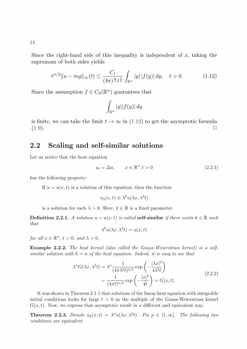
2.2 Scaling and self-similar solutions
Let us notice that the heat equation
ut = ∆u, x ∈ Rn, t > 0 (2.2.1)
has the following property:
If u = u(x, t) is a solution of this equation, then the function
uλ(x, t) ≡ λku(λx, λ2t)
is a solution for each λ > 0. Here, k ∈ R is a fixed parameter.
Definition 2.2.1. A solution u = u(x, t) is called self-similar if there exists k ∈ R suchthat
λku(λx, λ2t) = u(x, t)
for all x ∈ Rn, t > 0, and λ > 0.
Example 2.2.2. The heat kernel (also called the Gauss-Weierstrass kernel) is a self-similar solution with k = n of the heat equation. Indeed, it is easy to see that
λnG(λx, λ2t) = λn1
(4πλ2t)n/2exp
(−|λx|
2
4λ2t
)
=1
(4πt)n/2exp
(−|x|
2
4t
)= G(x, t).
(2.2.2)
It was shown in Theorem 2.1.1 that solutions of the linear heat equation with integrableinitial conditions looks for large t > 0 as the multiple of the Gauss-Weierstrass kernelG(x, t). Now, we express that asymptotic result in a different and equivalent way.
Theorem 2.2.3. Denote uλ(x, t) = λnu(λx, λ2t). Fix p ∈ [1,∞]. The following twoconditions are equivalent
15
1. limt→∞ t(n/2)(1−1/p)‖u(·, t)−MG(·, t)‖p = 0
2. for every t0 > 0,uλ(·, t0)→MG(·, t0), as λ→∞,
where the convergence is in the usual norm of Lp(Rn).
Proof. First, one should notice the following scaling property of the Lp-norm
‖v(λ·)‖p = λ−n/p‖v‖p, (2.2.3)
which can be easily proved by changing variables in the integral defining the norm.Now, using this scaling property together with identity (2.2.2) we obtain
The equivalence from Theorem 2.2.3 allows us to prove the asymptotic formula fromTheorem 2.1.1 in a different way. During these lectures, this idea will be called the FourStep Method and it will be used to show asymptotic properties of solutions to nonlinearequations. Now, we sketch the new proof of Theorem 2.1.1 based on the Four StepsMethod.
Step 1. Scaling. We introduce the rescaled family of functions
uλ(x, t) = λnu(λx, λ2t) for every λ > 0.
This is usually the most difficult part of this method: we have to choose the proper scalingof the model, which we study.
Step 2. Estimates and compactness. We show that the embedding
uλ(·, t)λ>0 ⊂ Lp(Rn) is compact for every t > 0.
Here, we derive those estimates using equation satisfied by uλ.
Step 3. Passage to the limit. By compactness there exists a sequence λn →∞ and afunctions u(x, t) such that
uλn(·, t)→ u(·, t) in Lp(Rn) for every t > 0.
Since uλ satisfies the heat equation (2.2.1), one can show that u is a weak solution of theheat equation, as well.
Step 4. Identification of the limit. The limit function u corresponds to Mδ0 (the Diracdelta) as an initial condition. The is the consequence of the the following lemma.
16
Lemma 2.3.1. Let u0 ∈ L1(Rn). For every test function ϕ ∈ C∞c (Rn) we have
∫
Rnλnu0(λx)ϕ(x) dx→Mϕ(0) as λ→∞,
where M =∫Rn u0(x) dx.
Proof. This is an immediate consequence of the Lebesgue dominated convergence theorem,because ∫
Rnλnu0(λx)ϕ(x) dx =
∫
Rnu0(x)ϕ(x/λ) dx,
by a simple change of variables.
Now, since the singular initial value problem (1.4.1)-(1.4.2) has a unique weak solutionby Theorem 1.4.1, we immediately obtain that
u(x, t) = MG(x, t).
Moreover, by the uniqueness of the limit, we have the following limit relation for the wholefamily
uλ(·, t)→MG(·, t) in Lp(Rn) for every t > 0.
Now, it suffices to use the equivalence from Theorem 2.2.3, to complete the proof ofTheorem 2.1.1.
Conclusion. This Four Steps Method is very useful to study asymptotic properties ofsolutions to nonlinear partial differential equations. We show details of this reasoning ina much more general case. Detailed proofs of results stated in Steps 1-4 in the case of thelinear heat equation can be found in [9, Ch. 1].
Chapter 3
Self-similar asymptotics of solutionsto convection-diffusion equation
3.1 The initial value problem
We are going to show the Four Step Method “in action”, by applying it to the initial valueproblem for the nonlinear convection diffusion equation
ut − uxx + (uq)x for x ∈ R, t > 0, (3.1.1)
u(x, 0) = u0(x) for x ∈ R, (3.1.2)
where q > 1 is a fixed parameter.
3.2 Existence of solutions
Let us first sketch proof on the global-in-time existence of solutions to problem (3.1.1)-(3.1.2).
Theorem 3.2.1 (Existence of global-in-time solution). Assume that
u0 ∈ L1(R) ∩ L∞(R) ∩ C(R). (3.2.1)
Suppose also that u0 ≥ 0. Then the initial value problem (3.1.1)–(3.1.2) has a nonnegative,global-in-time solution u ∈ C2,1(R × (0,∞)). This solution has the following regularityproperty
u ∈ C1((0,∞), Lp(R)) ∩ C((0,∞),W 2,p(R)))
for each p ∈ [1,∞]. Moreover, the solution conserves the integral (“mass”)
M ≡ ‖u(t)‖1 =
∫
Ru(x, t) dx =
∫
Ru0(x) dx = ‖u0‖1 for all t ≥ 0. (3.2.2)
This is a unique solution in the class of functions satisfying supt>0 ‖u(t)‖1 <∞.
17
18
3.2.1 Local existence via the Banach contraction principle
We construct local-in-time mild solutions of (3.1.1)–(3.1.2) which are solutions of thefollowing integral equation
u(t) = G(·, t) ∗ u0 +
∫ t
0
∂xG(·, t− s) ∗ uq(s) ds (3.2.3)
with the heat kernel G(x, t) = (4πt)−1/2 exp(− |x|2/(4t)
). In our reasoning, we use the
following estimates which result immediately from the Young inequality for the convolu-tion:
‖G(·, t) ∗ f‖p ≤ Ct−12( 1
q− 1p)‖f‖q, (3.2.4)
‖∂xG(·, t) ∗ f‖p ≤ Ct−12( 1
q− 1p)−
12‖f‖q (3.2.5)
for every 1 ≤ q ≤ p ≤ ∞, each f ∈ Lq(R), and C = C(p, q) independent of t, f . Noticethat C = 1 in inequality (3.2.4) for p = q because ‖G(·, t)‖L1 = 1 for all t > 0.
Lemma 3.2.2 (Local existence). Assume that
u0 ∈ L1(R) ∩ L∞(R) ∩ C(R).
Then there exists T = T (‖u0‖1, ‖u0‖∞) > 0 such that the integral equation (3.2.3) has theunique solution in the space
YT = C([0, T ], L1(R)) ∩ C([0, T ], L∞(R)),
supplemented with the norm ‖u‖YT = sup0≤t≤T ‖u‖1 + sup0≤t≤T ‖u‖∞.Proof. Here, it suffices to apply the Banach contraction principle to the internal equation(3.2.3). For sufficiently small T the right hand side of this equation defines the contractionin the space YT . Details of such a reasoning, in the case of a slightly different equationcan be found in [15, 14].
3.2.2 Regularity and comparison principle
One can show that a local in time solution is nonnegative, if an initial condition is so.Moreover, this solution has the following regularity property
u ∈ C1((0,∞), Lp(R)) ∩ C((0,∞),W 2,p(R)))
for each p ∈ [1,∞].
3.2.3 Global-in-time solutions
Below, in the proof of Theorem 3.3.2, we show that the solution satisfies the following apriori estimates for each p ∈ [1,∞]:
‖u(·, t)‖p ≤ ‖u0‖p for all t > 0.
Hence, by a standard reasoning, we can show that the solution is global in time.
19
3.3 Self-similar large time behavior of solutions
The main result on the self-similar large time behavior of solutions to problem (3.1.1)–(3.1.2) is stated in the following theorem.
Theorem 3.3.1 (Self-similar asymptotics). Under the assumptions of Theorem 3.2.1,every solution u = u(x, t) of problem (3.1.1)–(3.1.2) has a self-similar asymptotic profileas t→∞. More precisely,
i. if q > 2, we have
t(1−1/p)/2‖u(t)−MG(t)‖p → 0 as t→∞ (3.3.1)
for every p ∈ [1,∞], where M =∫R u0(x) dx and G(x, t) = 1√
4πtexp
(− |x|2
4t
)is the
heat kernel.
ii. On the other hand, if q = 2, we have
t(1−1/p)/2‖u(t)− UM(t)‖p → 0 as t→∞ (3.3.2)
for every p ∈ [1,∞], where UM(x, t) = 1√tUM(x√t, 1)
is the so-called nonlinear dif-fusion wave and is defined as the unique self-similar solution of the initial valueproblem for the viscous Burgers equation
Ut = Uxx −(U2)x, for x ∈ R, t > 0, (3.3.3)
U(x, 0) = Mδ0, (3.3.4)
where δ0 is the Dirac measure.
Let us recall properties of solutions to (3.3.3)-(3.3.4) which will be useful in the proofof Theorem 3.3.1. It is well-known that the Hopf-Cole transformation allows us to solvethis initial value problem to obtain the following explicit solution
UM(x, t) =t−1/2 exp (−|x|2/(4t))
CM + 12
∫ x/√t0
exp (−ξ2/4) dξ, (3.3.5)
where CM is a constant which is determined uniquely as a function of M by the condition∫R UM,A(η, 1) dη = M . The important point to note here is that for every M ∈ R the
function UM is a unique solution to equation (3.3.3) in the space C((0,∞);L1(R)) havingthe properties ∫
RUM(x, t) dx = M for all t > 0
and ∫
RUM(x, t)ϕ(x) dx→Mϕ(0) as t→ 0
for all ϕ ∈ C∞c (R) ([6, Sec. 4]). Such a solution is called a fundamental solution in thelinear theory and a source solution in the nonlinear case (cf. [7, 6]).
20
3.3.1 Rescaled family of functions
In the proof of Theorem 3.3.1, we study the behavior, as λ → ∞, of the rescaled familyof functions
uλ(x, t) = λu(λx, λ2t) for every λ > 0, (3.3.6)
which satisfy the initial value problems
∂tuλ = ∂2xuλ − λ2−q∂xuqλ, (3.3.7)
uλ(x, 0) = u0,λ(x) = λu0(λx). (3.3.8)
Notice that if u = u(x, t) is a nonnegative solution of problem (3.1.1)–(3.1.2) obtained inTheorem 3.2.1, then by (3.2.2) and by a simple change of variables, the following identity
‖uλ(t)‖1 = ‖u0‖1 (3.3.9)
holds true for all t > 0 and all λ > 0.
3.3.2 Optimal Lp-decay of solutions
Theorem 3.3.2. Under the assumptions of Theorem 3.2.1, the solution of problem (3.1.1)–(3.1.2) satisfies
‖u(·, t)‖p ≤ Ct−(1−1/p)/2‖u0‖1for each p ∈ [1,∞], a constant C = C(p) and all t > 0.
Proof. We sketch the proof for p = 2, only. Other p ∈ [1,∞] can be treated in a completelyanalogous way, see eg. [14, Thm. 2.3] and [11, Lemma 5.1].
Multiplying equation (3.1.1) by u and integrating the resulting equation over R wehave
1
2
d
dt
∫
Ru2 dx = −
∫
R|ux|2 dx. (3.3.10)
Here, we have used an elementary equalities
∫
Ruqx(x, t)u(x, t) dx =
1
q + 1
∫
R(uq+1(x, t))x dx = 0
if u(x, t)→ 0 when |x| → ∞.Now, by the Nash inequality
‖v‖2 ≤ C‖vx‖1/32 ‖v‖2/31 , (3.3.11)
which is valid for all v ∈ L1(R) such that vx ∈ L2(R), (since the L1-norm of the solutionis constant in time by (3.2.2)) we obtain the differential inequality
d
dt‖u(t)‖22 + C‖u0‖−41
(‖u(t)‖22
)3 ≤ 0, (3.3.12)
which implies ‖u(t)‖2 ≤ Ct−1/4 for all t > 0 and C > 0 independent of t.
21
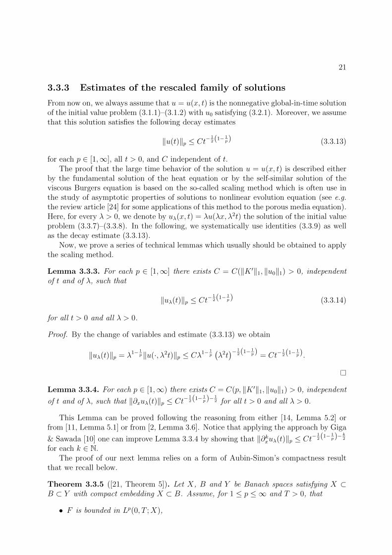
3.3.3 Estimates of the rescaled family of solutions
From now on, we always assume that u = u(x, t) is the nonnegative global-in-time solutionof the initial value problem (3.1.1)–(3.1.2) with u0 satisfying (3.2.1). Moreover, we assumethat this solution satisfies the following decay estimates
‖u(t)‖p ≤ Ct−12(1− 1
p) (3.3.13)
for each p ∈ [1,∞], all t > 0, and C independent of t.The proof that the large time behavior of the solution u = u(x, t) is described either
by the fundamental solution of the heat equation or by the self-similar solution of theviscous Burgers equation is based on the so-called scaling method which is often use inthe study of asymptotic properties of solutions to nonlinear evolution equation (see e.g.the review article [24] for some applications of this method to the porous media equation).Here, for every λ > 0, we denote by uλ(x, t) = λu(λx, λ2t) the solution of the initial valueproblem (3.3.7)–(3.3.8). In the following, we systematically use identities (3.3.9) as wellas the decay estimate (3.3.13).
Now, we prove a series of technical lemmas which usually should be obtained to applythe scaling method.
Lemma 3.3.3. For each p ∈ [1,∞] there exists C = C(‖K ′‖1, ‖u0‖1) > 0, independentof t and of λ, such that
‖uλ(t)‖p ≤ Ct−12(1− 1
p) (3.3.14)
for all t > 0 and all λ > 0.
Proof. By the change of variables and estimate (3.3.13) we obtain
‖uλ(t)‖p = λ1−1p‖u(·, λ2t)‖p ≤ Cλ1−
1p(λ2t)− 1
2(1− 1p) = Ct−
12(1− 1
p).
Lemma 3.3.4. For each p ∈ [1,∞) there exists C = C(p, ‖K ′‖1, ‖u0‖1) > 0, independent
of t and of λ, such that ‖∂xuλ(t)‖p ≤ Ct−12(1− 1
p)−12 for all t > 0 and all λ > 0.
This Lemma can be proved following the reasoning from either [14, Lemma 5.2] orfrom [11, Lemma 5.1] or from [2, Lemma 3.6]. Notice that applying the approach by Giga
& Sawada [10] one can improve Lemma 3.3.4 by showing that ‖∂kxuλ(t)‖p ≤ Ct−12(1− 1
p)−k2
for each k ∈ N.The proof of our next lemma relies on a form of Aubin-Simon’s compactness result
that we recall below.
Theorem 3.3.5 ([21, Theorem 5]). Let X, B and Y be Banach spaces satisfying X ⊂B ⊂ Y with compact embedding X ⊂ B. Assume, for 1 ≤ p ≤ ∞ and T > 0, that
• F is bounded in Lp(0, T ;X),
22
• ∂tf : f ∈ F is bounded in Lp(0, T ;Y ).
Then F is relatively compact in Lp(0, T ;B) (and in C(0, T ;B) if p =∞).
Lemma 3.3.6 (Compactness in L1loc(R) ). For every 0 < t1 < t2 <∞ and every R > 0,
the set uλλ>0 ⊆ C([t1, t2], L1([−R,R])) is relatively compact.
Proof. We apply Theorem 3.3.5 with p =∞, F = uλλ>0, and
X = W 1,1([−R,R]), B = L1([−R,R]), Y = W−1,1([−R,R]),
where R > 0 is fixed and arbitrary, and Y is the dual space of W 1,10 ([−R,R]). Obviously,
the embedding X ⊆ B is compact by the Rellich-Kondrashov theorem.By Lemmas 3.3.3 and 3.3.4 with p = 1, the sets uλλ>0 ⊆ L∞ ([t1, t2], L
1([−R,R]))and ∂xuλλ>0 ⊆ L∞ ([t1, t2], L
1([−R,R])) are bounded.To check the second condition of Aubin-Simon’s compactness criterion, it is suffices
to show that there is a positive constant C which independent of λ > 0 such thatsupt∈[t1,t2] ‖∂tuλ‖Y ≤ C. Here, it suffices to use the duality argument, see [14, Lemma5.5]. Hence, Lemma 3.3.6 is proved.
Lemma 3.3.7 (Compactness in L1(R) ). For every 0 < t1 < t2 <∞, the set uλλ>0 ⊆C([t1, t2], L
1(R)) is relatively compact.
Proof. Let ψ ∈ C∞(R) be nonnegative and satisfy ψ(x) = 0 for |x| < 1 and ψ(x) = 1 for|x| > 2. Put ψR(x) = ψ(x/R) for every R > 0. Since u is nonnegative, in view of Lemma3.3.6, using a standard diagonal argument, it suffices to show that
supt∈[t1,t2]
‖uλ(t)ψR‖1 → 0 as R→∞, uniformly in λ ≥ 1. (3.3.15)
Hence, multiplying the both sides of equation (3.3.7) by ψR and integrating over R andfrom 0 to t, we complete the proof as in [14, Lemma 5.6], [2, Lemma 3.10].
Lemma 3.3.8 (Initial condition). For every test function φ ∈ C∞c (R), there exists C =C(φ, ‖K ′‖1, ‖u0‖1) independent of λ such that
∣∣∣∣∫
Ruλ(x, t)φ(x) dx−
∫
Ru0,λ(x)φ(x) dx
∣∣∣∣ ≤ C(t+ t1/2
). (3.3.16)
Proof. Here, it suffices to follow [2, Lemma 3.9] and [14, Lemma 5.7]
Now, we are in a position to prove our main result on the large time behavior ofsolutions to problem (3.1.1)-(3.1.2).
Proof of Theorem 3.3.1. By Lemma 3.3.7, for every 0 < t1 < t2 <∞, the family uλλ>0
is relatively compact in C([t1, t2], L1(R)) for any 0 < t1 < t2 < ∞. Consequently, there
exists a subsequence of uλλ>0 (not relabeled) and a function u ∈ C((0,∞), L1(R)) suchthat
uλ → u in C([t1, t2], L1(R)) as λ→∞. (3.3.17)
23
Passing to a subsequence, we can assume that
uλ(x, t)→ u(x, t) as λ→∞ (3.3.18)
almost everywhere in (x, t) ∈ R× (0,∞).Now, multiplying equation (3.3.7) by a test function φ ∈ C∞c (R × (0,∞)) and inte-
grating the resulting equation over R× (0,∞), we obtain the identity
−∫
R
∫ ∞
0
uλφt dsdx =
∫
R
∫ ∞
0
uλφxx dsdx+ λ2−q∫
R
∫ ∞
0
uqλφx dsdx. (3.3.19)
Therefore, passing to the limit λ→∞ in equality (3.3.19) and using the properties of thesequence uλλ>0 stated in (3.3.17) and (3.3.18), we obtain that u(x, t) is a weak solutionof the equation
ut = uxx − (u2)x
if q = 2.Now, notice that, by the change of variables and the dominated convergencetheorem, we obtain
∫R u0,λ(x)φ(x) dx =
∫R u0(x)φ(x/λ) dx → Mφ(0) as λ → ∞. Hence,
it follows from Lemma 3.3.8 that u(x, 0) = Mδ0 in the sense of bounded measures. Thus,u is a weak solution of the initial value problem
ut = uxx − (u2)x, (3.3.20)
u(x, 0) = Mδ0. (3.3.21)
Since problem (3.3.20)-(3.3.21) has a unique solution (see e.g. [6, Sec. 4]), the wholefamily uλλ>0 converge to u in C((0,∞), L1(R)).
Obviously, if q > 2, this limit function is a solution to the linear problem
ut = uxx, (3.3.22)
u(x, 0) = Mδ0. (3.3.23)
So, it is the multiple of Gauss-Weierstrass kernel
u(x, t) = MG(x, t) = M1√4πt
exp(− |x|
2
4t
). (3.3.24)
Hence, by (3.3.17), we have
limλ→∞‖uλ(1)− u(1)‖1 = 0
and, after setting λ =√t and using the self-similar form of u(x, t) = t−1/2u(xt−1/2, 1), we
obtainlimt→∞‖u(t)− u(t)‖1 = 0. (3.3.25)
The convergence of u(·, t) towards the self-similar profile in the Lp-norms for p ∈ (1,∞)is the immediate consequence of the Holder inequality, the decay estimate (3.3.13) withp =∞, and (3.3.25). Indeed, we have
‖u(t)− u(t)‖p ≤(‖u(t)‖∞ + ‖u(t)‖∞
)1−1/p‖u(t)− u(t)‖1/p1 = o(t−(1−1/p)/2) (3.3.26)
24
as t→∞.To complete the proof of Theorem 3.3.1, it remains to show the convergence in the L∞-
norm. Here, however, it suffices notice the decay estimate ‖ux(t)‖2 ≤ Ct−3/4, providedby Lemma 3.3.4 with λ = 1, and the identity ‖ux(t)‖2 = t−3/4‖ux(1)‖2 resulting fromthe explicit formulas (3.3.24) and (3.3.5). Hence, by the Gagliardo-Nirenberg-Sobolevinequality and by (3.3.26) with p = 2, we obtain
‖u(t)− u(t)‖∞ ≤ C(‖ux(t)‖2 + ‖ux(t)‖2
)1/2‖u(t)− u(t)‖1/22 = o(t−1/2)
as t→∞.
Chapter 4
Pseudo-measures and large timeasymptoics
4.1 Statement of the problem
In this chapter, we shall describe a method invented by M. Cannone and the author ofthese lecture notes [4] which allows to construct global-in-time solutions for small initialconditions. In this approach, self-similar solutions and stationary solutions are treatten inthe same way. In the following, we consider the initial value problem for the converction-diffusion equation
ut −∆u+ a · ∇u2 = F, x ∈ R3, t > 0 (4.1.1)
u(0) = u0. (4.1.2)
Here, F = F (x, t) is a given function and a ∈ R3 is a fixed vector.
4.1.1 Navier–Stokes equations
In [4], in fact, we consider the famous Navier–Stokes equations, describing the evolutionof the velocity field u and pressure p of a three-dimensional incompressible viscous fluidat time t and the position x ∈ R3. These equations are given by
ut −∆u+ (u · ∇)u+∇p = F, (4.1.3)
∇ · u = 0, (4.1.4)
u(0) = u0. (4.1.5)
where the external force F and initial velocity u0 are assigned.In [4], we study global-in-time solutions u = u(x, t) to the Cauchy problem in R3 for
the incompressible Navier–Stokes equations (4.1.3)–(4.1.4). As far as u = u(x, t) is asufficiently regular function, the equations (4.1.3)–(4.1.4) can be rewritten as
ut −∆u+∇ · (u⊗ u) +∇p = F, ∇ · u = 0.
25
26
If we recall that the Leray projector on solenoidal vector fields is given by the formula
Pv = v −∇∆−1(∇ · v) (4.1.6)
for sufficiently smooth functions v = (v1(x), v2(x), v3(x)), we formally transform the sys-tem (4.1.1)–(4.1.4) into
ut −∆u+ P∇ · (u⊗ u) = PF, ∇ · u = 0.
To give a meaning to the Leray projector P (defined in (4.1.6)), let us first recallthat the Riesz transforms Rj are the pseudodifferential operators defined in the Fourier
variables as Rkf(ξ) = iξk|ξ| f(ξ). Here and in what follows the Fourier transform of an
integrable function v is given by v(ξ) ≡ (2π)−n/2∫Rn e
−ix·ξv(x) dx. Using these well-known operators we define
(Pv)j = vj +3∑
k=1
RjRkvk;
moreover, in our considerations below, we shall often denote by P(ξ) the symbol of thepseudodifferential operator P which is the matrix with components
(P(ξ))j,k = δjk −ξjξk|ξ|2 .
All these components are bounded on R3, more precisely, we have
max1≤j,k≤3
supξ∈R3\0
|(P(ξ))j,k| = 1. (4.1.7)
To present the main ideas from [4], we limitt ourselves in these lecture notes to thesimpler problem (4.1.1)–(4.1.2).
4.2 Definitions and spaces
First, let us emphasize that we shall study the problem (4.1.1)–(4.1.2) via the followingintegral equation obtained from the Duhamel principle
u(t) = S(t)u0 −∫ t
0
S(t− τ)a · ∇u2(τ) dτ (4.2.1)
+
∫ t
0
S(t− τ)F (τ) dτ,
where S(t) is the heat semigroup given as the convolution with the Gauss–Weierstrasskernel: G(x, t) = (4πt)−3/2 exp(−|x|2/(4t)).
We are now in a position to introduce the Banach functional spaces relevant to ourstudy of solutions of the Cauchy problem for the system (4.1.1)–(4.1.2):
PMa ≡ v ∈ S ′(Rd) : v ∈ L1loc(Rd), ‖v‖PMa ≡ ess sup
ξ∈R3
|ξ|a|v(ξ)| <∞,
27
where a ∈ [0, 3) is a given parameter. The notation PM stands for pseudomeasure,and the classical space of pseudomeasures introduced in harmonic analysis (i.e. thosedistributions whose Fourier transforms are bounded) corresponds to a = 0.
Definition 4.2.1. By a solution of (4.1.1)–(4.1.2) we mean in this chapter a functionu = u(x, t) belonging to the space X = Cw([0, T );PM2), 0 < T ≤ ∞, and such that
u(ξ, t) = e−t|ξ|2
u(ξ, 0) +
∫ t
0
e−(t−τ)|ξ|2
ia · ξ(u2)
(ξ, τ) dτ (4.2.2)
+
∫ t
0
e−(t−τ)|ξ|2
F (ξ, τ) dτ
for all 0 ≤ t ≤ T .
Remark 2.1 Given f ∈ S ′(R3) ∩ L1loc(R3) we denote the rescaling fλ(x) = f(λx). In
a standard way, we extend this definition to all tempered distributions. It follows fromelementary calculations that fλ(ξ) = λ−3f(λ−1ξ). Hence, for every λ > 0, we obtain thescaling property of the norm in PMa
‖fλ‖PMa = λa−3‖f‖PMa . (4.2.3)
In particular, the norm PM2 is invariant under rescaling f 7→ λf(λ ·). Moreover, itfollows from (4.2.3) that for a = 3(1 − 1/p) the norms ‖ · ‖PMa and ‖ · ‖Lp(R3) have thesame scaling property.
Remark 2.2 The letter Cw denotes, as usual (cf. [3]), the space of vector-valued functionswhich are weakly continuous as distributions in t. This is an additional difficulty causedby the fact that the heat semigroup (S(t))t≥0 is not strongly continuous on the spaces ofpseudomeasures but only weakly continuous (cf. Lemma 4.3.2, below).
Remark 2.3 Usually, a mild solution of an evolution equation like (4.1.1)–(4.1.2) is definedas a solution to the integral equation (4.2.1) and the integral is understood as the Bochnerintegral.
Nevertheless, a distributional solution of system (4.1.1)–(4.1.2) is a solution of theintegral equation of (4.2.2), and vice versa. This equivalence can be proved by a stan-dard reasoning, and we refer the interested reader to [25, Th. 5.2] for details of suchcomputations.
To simplify the notation, the quadratic term in (4.2.1) will be denoted by
B(u, v)(t) = −∫ t
0
S(t− τ)a · ∇u(τ)v(τ) dτ, (4.2.4)
where u = u(t) and v = v(t) are functions defined on [0, T ) with values in a vector space(here most frequently PM2).
28
4.3 Global-in-time solutions
4.3.1 Construction of solutions
The proof of our basic theorem on the existence, uniqueness and stability of solutions tothe problem (4.1.1)–(4.1.2) is based on the following abstract lemma, whose slightly moregeneral form is taken from [17].
Lemma 4.3.1. Let (X , ‖ · ‖X ) be a Banach space and B : X ×X → X a bounded bilinearform satisfying ‖B(x1, x2)‖X ≤ η‖x1‖X‖x2‖X for all x1, x2 ∈ X and a constant η > 0.Then, if 0 < ε < 1/(4η) and if y ∈ X such that ‖y‖ < ε, the equation x = y+B(x, x) hasa solution in X such that ‖x‖X ≤ 2ε. This solution is the only one in the ball B(0, 2ε).Moreover, the solution depends continuously on y in the following sense: if ‖y‖X ≤ ε,x = y +B(x, x), and ‖x‖X ≤ 2ε, then
‖x− x‖X ≤1
1− 4ηε‖y − y‖X .
Proof. Here, the reasoning is based on the standard Picard iteration technique completedby the Banach fixed point theorem. For other details of the proof, we refer the reader to[17, Th. 13.2].
Our goal is to apply Lemma 4.3.1 in the space
X = Cw([0,∞),PM2) (4.3.1)
to the integral equation (4.2.1) which has the form u = y + B(u, u), where the bilinearform is defined in (4.2.4) and y = S(t)u0 +
∫ t0S(t− τ)F (τ) dτ . We need some preliminary
estimates.
Lemma 4.3.2. Given u0 ∈ PM2, we have S(·)u0 ∈ X .
Proof. By the definition of the norm in PM2, it follows that
‖S(t)u0‖PM2 = ess supξ∈R3
|ξ|2∣∣∣e−t|ξ|2u0(ξ)
∣∣∣ ≤ ess supξ∈R3
|ξ|2|u0(ξ)| = ‖u0‖PM2 ,
so, S(·)u0 ∈ L∞([0,∞),PM2).Now, let us prove the weak continuity with respect to t, and, by the semigroup property
of S(t), it suffices to do this for t = 0 only. For every ϕ ∈ S(R3), by the Plancherel formula,we obtain
|〈S(t)u0 − u0, ϕ〉| =
∣∣∣∣∫ (
e−t|ξ|2 − 1
)u0(ξ)ϕ(ξ) dξ
∣∣∣∣
≤ t ess supξ∈R3
∣∣∣∣∣e−t|ξ|
2 − 1
t|ξ|2
∣∣∣∣∣ ‖u0‖PM2‖ϕ‖L1R3 → 0 as t 0.
29
Lemma 4.3.3. Given F ∈ Cw([0,∞),PM), it follows that
w ≡∫ t
0
S(t− τ)F (τ) dτ ∈ X .
Moreover, ‖w‖X ≤ ‖F‖Cw([0,∞),PM).
Proof. Similarly as in the proof of Lemma 4.3.2 we get
‖w(t)‖PM2 = ess supξ∈R3
|ξ|2∣∣∣∣∫ t
0
e−(t−τ)|ξ|2
F (ξ, τ) dτ
∣∣∣∣
≤ |ξ|2∫ t
0
e−(t−τ)|ξ|2
dτ‖F‖Cw([0,∞),PM)
≤ ‖F‖Cw([0,∞),PM).
Let us skip the proof of the weak continuity of w(t) because the reasoning is more or lessstandard. Similar arguments can be found e.g. either in [19, Ch. 18, Lemma 24] or in [25,Th. 3.1].
The goal of the next proposition is to prove that the bilinear form B(·, ·) defined in(4.2.4) is continuous on the space X = Cw([0,∞),PM2).
Proposition 4.3.4. The bilinear operator B(·, ·) is continuous on the space X defined in(4.3.1). Hence, there exists a constant η > 0 such that for every u, v ∈ X , it follows
‖B(u, v)‖X ≤ η‖u‖X‖v‖X .Proof. We do all the calculations in the Fourier variables and we use equation (4.1.7).Using elementary properties of the Fourier transform we obtain
∣∣∣(uv)(ξ, τ)∣∣∣ ≤ C
∫
R3
dz
|ξ − z|2|z|2 ‖u(τ)‖PM2‖v(τ)‖PM2
=η
|ξ|‖u(τ)‖PM2‖v(τ)‖PM2 .
In the computations above, we use the equality |ξ|−2 ∗ |ξ|−2 = π3|ξ|−1. A detailed analysisconcerning such convolutions can be found in [18, Th. 5.9] or [22, Ch. V, Sec.1, (8)].
Now, the boundedness of the bilinear form on X results from the following estimates
|ξ|2∣∣∣∣∫ t
0
e−(t−τ)|ξ|2
ia · ξ · (uv)(ξ, τ)
∣∣∣∣ dτ
≤ η|ξ|2∫ t
0
e−(t−τ)|ξ|2
dτ ‖u‖X‖v‖X≤ η‖u‖X‖v‖X .
It remains to show the weak continuity of B(u, v)(t) with respect to t, but this followsagain from standard arguments, cf. the remark at the end of the proof of Lemma 4.3.3.
Now, the main theorem of this section results immediately from Lemma 4.3.1 combinedwith Lemmata 4.3.2–4.3.3 and Proposition 4.3.4.
30
Theorem 4.3.5. Assume that u0 ∈ PM2 and F ∈ Cw([0,∞),PM) satisfy ‖u0‖PM2 +‖F‖Cw([0,∞),PM) < ε for some 0 < ε < 1/(4η) where η is defined in Proposition 4.3.4.There exists a global-in-time solution of (4.1.1)–(4.1.2) in the space X = Cw([0,∞),PM2).This is the unique solution satisfying the condition ‖u‖Cw([0,∞),PM2) ≤ 2ε. Moreover,this solution depends continuously on initial data and external forces in the sense ofLemma 4.3.1.
4.3.2 Self-similar solutions
Assume, for a moment, that F ≡ 0. Homogeneity properties of the problem (4.1.1)–(4.1.4) imply that if u solves the Cauchy problem, then the rescaled function uλ(x, t) =λu(λx, λ2t) is also a solution for each λ > 0. Thus, it is natural to consider solutionswhich satisfy the scaling invariance property uλ ≡ u for all λ > 0, i.e. forward self-similar solutions. By the very definition, they are global-in-time, and one may expectthat they describe the large time behavior of general solutions of (4.1.1)–(4.1.2). Indeed,if limλ→∞ λu(λx, λ2t) = U(x, t) in an appropriate sense, then tu(xt1/2, t) → U(x, 1) ast → ∞ (take t = 1, λ = t1/2), and U ≡ Uλ is scale invariant. Hence U is a self-similarsolution, and
U(x, t) = t−1/2U(x/t1/2, 1) (4.3.2)
is thus determined by a function of d variables U(y) ≡ U(y, 1), y = x/t1/2 being theBoltzmann substitution.
If uλ ≡ u for all λ > 0, then from the self-similar form (4.3.2), the initial condition(4.1.2) limt0 u(x, t) is a distribution homogeneous of degree −1 at the origin.
Remark 3.1 Self-similar solutions can be obtained directly from Theorem 4.3.5 by takingu0 homogeneous of degree−1 of small PM2 norm. By the uniqueness property of solutionsof the Cauchy problem constructed in Theorem 4.3.5, they have the form (4.3.2).
The same reasoning can be applied to the case when external forces are present.Indeed, if the initial datum u0 is homogeneous of degree −1 and if the external forceF (x, t) satisfies
λ3F (λx, λ2t) = F (x, t) for all λ > 0 (4.3.3)
(here, the scaling is understood in the distributional sense), the solution obtained inTheorem 4.3.5 is self-similar. Note that, in particular, we can take
F (x, t) = F (x) = (b1δ0, b2δ0, b3δ0)
(the multiples of the Dirac delta) for sufficiently small |b|.Proceeding in this way we arrive at
Corollary 4.3.6. Suppose that the initial condition u0 ∈ PM2 is homogeneous of degree−1 and F ∈ Cw([0,∞),PM) satisfies (4.3.3). Let u0 and F satisfy, moreover, the assump-tions of Theorem 4.3.5. The corresponding unique solution constructed in Theorem 4.3.5is self-similar.
Remark 3.2 The self-similar solutions constructed in such a way can have singularitiesfor any time. This is the case, for instance, for the self-similar (stationary) solutions by
31
Landau and Tian and Xin described in [4]. On the other hand, when using the two normsapproach of Kato as in [3], the self-similar solutions that arise from this construction areinstantaneously smoothed out for t > 0 and the only singularity (of the type ∼ 1/|x|) canbe found at t = 0.
Remark 3.3 The existence and the stability results from this section are closely relatedto those from the paper by Yamazaki [25] where he studied the Navier–Stokes system inthe weak Lp-spaces in an exterior domain Ω. In those considerations, Yamazaki appliedthe Kato algorithm in the space Cw([0,∞), L3,∞(Ω)) without a priori assumptions on thedecay of solutions. Our approach involving the PM2 space is much more elementary thanthat from [25]. Moreover, we can treat more singular external forces, and we obtain akind of asymptotic stability of solutions (see the next section).
4.4 Asymptotic behavior of solutions
In our investigations concerning the large time behavior of solutions to problem (4.1.1)–(4.1.2) we need the following improvement of Lemma 4.3.3.
Lemma 4.4.1. Assume that F ∈ Cw([0,∞),PM) satisfies limt→∞ ‖F (t)‖PM = 0. Then
limt→∞
∥∥∥∥∫ t
0
S(t− τ)F (τ) dτ
∥∥∥∥PM2
= 0.
Proof. It follows from the definition of the norm ‖ · ‖PM2 and from (4.1.7) that∥∥∥∥∫ t
0
S(t− τ)F (τ) dτ
∥∥∥∥PM2
≤ supξ∈R3
∫ t
0
|ξ|2e−(t−τ)|ξ|2‖F (τ)‖PM dτ
≤ supξ∈R3
∫ t/2
0
... dτ + supξ∈R3
∫ t
t/2
... dτ.
Using the substitution ξ = w√t− τ , we first obtain
supξ∈R3
∫ t/2
0
|ξ|2e−(t−τ)|ξ|2‖F (τ)‖PM dτ ≤∫ t/2
0
(t− τ)−1 supw∈R3
|w|2e−|w|2‖F (τ)‖PM dτ
≤ C
∫ t/2
0
(t− τ)−1‖F (τ)‖PM dτ
= C
∫ 1/2
0
(1− s)−1‖F (ts)‖PM dτ.
Now, the right-hand side of the above inequality tends to 0 as t → ∞ by the LebesgueDominated Convergence Theorem.
We estimate the term containing the integral∫ tt/2... dτ in the most direct way by
(supξ∈R3
∫ t
t/2
|ξ|2e−(t−τ)|ξ|2 dτ)
supt/2≤τ≤t
‖F (τ)‖PM ≤ C supt/2≤τ≤t
‖F (τ)‖PM → 0
as t→∞ by the assumption on F .
32
Theorem 4.4.2. Let the assumptions of Theorem 4.3.5 hold true. Assume that u andv are two solutions of (4.1.1)–(4.1.2) constructed in Theorem 4.3.5 corresponding to theinitial conditions u0, v0 ∈ PM2 and external forces F,G ∈ Cw([0,∞),PM), respectively.Suppose that
limt→∞‖S(t)(u0 − v0)‖PM2 = 0 and lim
t→∞‖F (t)−G(t)‖PM = 0. (4.4.1)
Then
limt→∞‖u(·, t)− v(·, t)‖PM2 = 0 (4.4.2)
holds.
This result means that if the difference of the solutions of the heat equation issuedfrom u0, v0 becomes negligible as t→∞ (e.g., if the difference of the initial data u0−v0 isnot too singular) and if F (t) and G(t) have the same large time asymptotics, the solutionsof the nonlinear problem u(t), v(t) behave similarly for large times. It can be interpretedas a kind of asymptotic stability result if the choice of v0 is restricted to the initial datain a neighborhood of u0 satisfying additionally (4.4.1). It is easy to verify that the firstcondition in (4.4.1) is satisfied if, e.g., |ξ|2(u0(ξ)− v0(ξ))→ 0 as ξ → 0.
Proof of Theorem 4.4.2. First, let us recall that, by Theorem 4.3.5, we have
supt≥0‖u(t)‖PM2 ≤ 2ε <
1
2ηand sup
t≥0‖v(t)‖PM2 ≤ 2ε <
1
2η. (4.4.3)
We subtract the integral equation (4.2.1) for v from the analogous expression for u. Next,computing the norm ‖·‖PM2 of the resulting equation and repeating the calculations fromthe proof of Proposition 4.3.4 we obtain the following inequality
In the term on the right-hand side of (4.4.4) containing the integral∫ δt0... dτ , we
change the variables τ = ts and we use the identity
supξ∈R3
|ξ|2e−(1−s)t|ξ|2 = ((1− s)t)−1 supw∈R3
|w|2e−|w|2 = ((1− s)t)−1e−1
33
in order to estimate it by
η supξ∈R3
∫ δ
0
t|ξ|2e−(1−s)t|ξ|2‖u(ts)− v(ts)‖PM2 ds
×(
supτ>0‖u(τ)‖PM2 + sup
τ>0‖v(τ)‖PM2
)(4.4.5)
≤ 4εηe−1∫ δ
0
(1− s)−1‖u(ts)− v(ts)‖PM2 ds.
We deal with the term in (4.4.4) containing∫ tδt... dτ estimating it directly by
η
(supξ∈R3
∫ t
δt
|ξ|2e−(t−τ)|ξ|2 dτ)(
supδt≤τ≤t
‖u(τ)− v(τ)‖PM2
)4ε (4.4.6)
= 4εη supδt≤τ≤t
‖u(τ)− v(τ)‖PM2 ,
since supξ∈R3
∫ tδt|ξ|2e−(t−τ)|ξ|2 dτ = supξ∈R3
(1− e−(δt)|ξ|2
)= 1.
Now, we denote
g(t) = ‖S(t)(u0 − v0)‖PM2 +
∥∥∥∥∫ t
0
S(t− τ)(F (t)−G(t)) dτ
∥∥∥∥PM2
,
and it follows from the assumptions, (4.4.1) and Lemma 4.4.1 that
g ∈ L∞(0,∞) and limt→∞
g(t) = 0. (4.4.7)
Hence, applying (4.4.5) and (4.4.6) to (4.4.4) we obtain
‖u(t)− v(t)‖PM2 ≤ g(t) + 4εηe−1∫ δ
0
(1− s)−1‖u(ts)− v(ts)‖PM2 ds (4.4.8)
+4εη supδt≤τ≤t
‖u(τ)− v(τ)‖PM2
for all t > 0.Next, we put
A = lim supt→∞
‖u(t)− v(t)‖PM2 ≡ limk∈IN,k→∞
supt≥k‖u(t)− v(t)‖PM2 .
The number A is nonnegative and finite because both u, v ∈ L∞([0,∞),PM2), and ourclaim is to show that A = 0. Here, we apply the Lebesgue Dominated ConvergenceTheorem to the obvious inequality
supt≥k
∫ δ
0
(1− s)−1‖u(ts)− v(ts)‖PM2 ds ≤∫ δ
0
(1− s)−1 supt≥k‖u(ts)− v(ts)‖PM2 ds,
and we obtain
lim supt→∞
∫ δ
0
(1− s)−1‖u(ts)− v(ts)‖PM2 ds ≤ A
∫ δ
0
(1− s)−1 ds = A log
(1
1− δ
). (4.4.9)
34
Moreover, since
supt≥k
supδt≤τ≤t
‖u(τ)− v(τ)‖PM2 ≤ supδk≤τ<∞
‖u(τ)− v(τ)‖PM2 ,
we havelim supt→∞
supδt≤τ≤t
‖u(τ)− v(τ)‖PM2 ≤ A. (4.4.10)
Finally, computing lim supt→∞ of the both sides of inequality (4.4.8), and using (4.4.7),(4.4.9), and (4.4.10) we get
A ≤(
4εηe−1 log
(1
1− δ
)+ 4εη
)A.
Consequently, it follows that A = lim supt→∞ ‖u(t)− v(t)‖PM2 = 0 because
4εη
(e−1 log
(1
1− δ
)+ 1
)< 1,
for δ > 0 sufficiently small, by the assumption of Theorem 4.3.5 saying that 0 < ε <1/(4η). This completes the proof of Theorem 4.4.2.
As a direct consequence the proof of Theorem 4.4.2, we have also necessary conditionsfor (4.4.2) to hold. We formulate this fact in the following corollary.
Corollary 4.4.3. Assume that u, v ∈ Cw([0,∞),PM2) are solutions to system (4.1.1)–(4.1.2) corresponding to initial conditions u0, v0 ∈ PM2 and external forces F,G ∈Cw([0,∞),PM), respectively. Suppose that
limt→∞‖u(t)− v(t)‖PM2 = 0. (4.4.11)
Then
limt→∞
∥∥∥∥S(t)(u0 − v0) +
∫ t
0
S(t− τ)(F (τ)−G(τ)) dτ
∥∥∥∥PM2
= 0.
Proof. As in the beginning of the proof of Theorem 4.4.2, we subtract the integral equation(4.2.1) for v from the same expression for u, and we compute the PM2-norm
The first term on the right-hand side of (4.4.12) tends to zero as t→∞ by (4.4.11). Toshow the decay of the second one, it suffices to repeat calculations from (4.4.4), (4.4.5),(4.4.6), and (4.4.9). Here, however, one should remember that now it is assumed thatA = 0 and supt>0 ‖u(t)‖PM2 <∞ and supt>0 ‖v(t)‖PM2 <∞.
35
Remark 4.1 In the setting of the Lp-spaces and the homogeneous Besov spaces, the studyof the asymptotic stability of self-similar solutions to the Navier–Stokes system begunwith the paper [20] of F. Planchon (see also the presentation of Planchon’s results in [17,Ch. 23.3]). As illustrated in the book by Y. Giga and M.-H. Giga [?] those ideas are quiteuniversal and were used for other partial differential equations (e.g. the porous medium,the nonlinear Schrodinger and the KdV equations); they were applied for instance tostudy asymptotic properties of solutions to a large class of nonlinear parabolic equations[11] as well as of solutions with zero mass to viscous conservation laws [13]. In this section,we extend them on solutions which not necessarily decay to 0 as t→∞.
4.5 Stationary solutions
Our approach, described in previous sections, to study global-in-time solutions to theproblem (4.1.1)–(4.1.2), as well as their large time behavior, can be also applied to sta-tionary solutions. Below, we briefly describe some consequences of Theorems 4.3.5 and4.4.2. The following proposition contains two equivalent integral equations satisfied bystationary solutions.
Proposition 4.5.1. Assume that u = u(x) ∈ PM2 and F ∈ PM. The following twofacts are equivalent
1) u = u(x) is a stationary mild solution of system (4.1.1)–(4.1.4) in the sense ofDefinition 4.2.1. Hence, u is the solution of the integral equation
u = S(t)u−∫ t
0
S(t− τ)a · ∇u2 dτ +
∫ t
0
S(τ)F dτ (4.5.1)
for every t > 0;
2) u satisfies the integral equation
u = −∫ ∞
0
S(τ)a · ∇u2 dτ +
∫ ∞
0
S(τ)F dτ, (4.5.2)
where the integrals above should be understood in the Fourier variables for almostevery ξ.
Proof. By Definition 4.2.1, the integral equation (4.5.1) can be rewritten as
u(ξ) = e−t|ξ|2
u(ξ)−∫ t
0
e−(t−τ)|ξ|2
dτ ia · ξ(u2)(ξ)
+
∫ t
0
e−(t−τ)|ξ|2
dτ F (ξ) (4.5.3)
= e−t|ξ|2
u(ξ)− 1− e−t|ξ|2
|ξ|2 ia · ξ(u2)(ξ) +1− e−t|ξ|2
|ξ|2 F (ξ).
for every t > 0. Passing to the limit as t→∞ in (4.5.3) and using the identity
1
|ξ|2 =
∫ ∞
0
e−τ |ξ|2
dτ for ξ 6= 0,
36
we obtain equation (4.5.2) in the Fourier variables.
Now, assume that u solves (4.5.2). Repeating the arguments above in the reverseorder, we obtain that u is the solution of the equation
u(ξ) = − 1
|ξ|2 (ξ)ia · ξ(u2)(ξ) +1
|ξ|2 F (ξ). (4.5.4)
If we subtract from this equality the same expression multiplied by e−t|ξ|2
we get (4.5.3)which obviously is equivalent to (4.5.1).
Theorem 4.5.2. Assume that F ∈ PM satisfies ‖F‖PM < ε < 1/(4η). There existsa stationary solution u∞ to the Navier–Stokes system in the space PM2 with F as theexternal force. This is the unique solution satisfying the condition ‖u‖PM2 ≤ 2ε.
Proof. This theorem results immediately from Lemma 4.3.1 applied to the integral equa-tion (4.5.2) (or its equivalent version (4.5.4)). The bilinear form
B(u, v) =
∫ ∞
0
S(τ)a · ∇uv dτ
is bounded on the space PM2 and the proof of this property of B(·, ·) is completelyanalogous to the one of Proposition 4.3.4. Let us also skip an easy proof that y =∫∞0S(τ)F dτ satisfies ‖y‖PM2 = ‖F‖PM.
Now, the application of Theorem 4.4.2 gives the following result on the asymptoticstability of stationary solutions.
Corollary 4.5.3. Assume that u∞ is the stationary solution constructed in Theorem 4.5.2corresponding to the external force F . Suppose that v0 ∈ PM2 and G ∈ Cw([0,∞),PM)satisfy ‖v0‖PM2 + ‖G‖Cw([0,∞),PM) ≤ ε < 1/(4η) and, moreover,
limt→∞‖S(t)(v0 − u∞)‖PM2 = 0, lim
t→∞‖G(t)− F‖PM = 0.
Then, the solution v = v(x, t) of system (4.1.1)–(4.1.2) corresponding to v0 and G con-verges toward the stationary solution u∞ in the following sense
limt→∞‖v(t)− u∞‖PM2 = 0.
Proof. Here, it suffices only to note that stationary solutions belong to the space
Cw([0,∞),PM2)
(treated as constant functions on [0,∞) with values in PM2) and satisfy the integralequation (4.2.1) (see Proposition 4.5.1). So, Theorem 4.4.2 is applicable in this case.
37
4.6 Smooth solutions
Solutions of problem (4.1.1)–(4.1.2) constructed in the space X = Cw([0,∞),PM2) are,in fact, more regular for sufficiently regular external forces. The goal of this section isto clarify this remark. First, let us recall that, in [3], solutions of (4.1.1)–(4.1.2) wereconstructed for sufficiently small initial conditions from the homogeneous Besov spaceB−1+3/p,∞p (R3) with 3 < p <∞. The usual way of defining a norm in this space is based
on the dyadic decomposition of tempered distributions. Here, however as in [11] we preferthe equivalent norm whose definition involves the heat semigroup
‖v‖B−α,∞p (R3) ≡ supt>0
tα/2‖S(t)v‖Lp(R3).
Connections between PM2 and homogeneous Besov spaces are described in the followinglemma.
Lemma 4.6.1. For every p ∈ (3,∞] the following imbeddings PM2 ⊂ B−1+3/p,∞p (R3)
hold true and are continuous. Hence, there exists a constant C = C(p) such that
supt>0
t(1−3/p)/2‖S(t)u0‖Lp(R3) ≤ C‖u0‖PM2
for all t > 0 and u0 ∈ PM2.
Proof. Here, our tool is the Hausdorff–Young inequality. For 1/p+ 1/q = 1 we obtain
‖S(t)u0‖qLp(R3) ≤ C
∫
R3
∣∣∣e−t|ξ|2u0(ξ)∣∣∣q
dξ
≤ C
(ess supξ∈R3
|ξ|2|u0(ξ)|)q ∫
R3
∣∣∣∣∣e−qt|ξ|
2
|ξ|2q
∣∣∣∣∣ dξ
= C‖u0‖qPM2t−3/2+q
∫
R3
∣∣∣∣∣e−q|w|
2
|w|2q
∣∣∣∣∣ dw.
In the calculations above, we assume that 2q < 3 which is equivalent to p > 3. Since,1/q = 1− 1/p and (3/2)(1− 1/p)− 1 = (1/2)(1− 3/p), we obtain
t(1/2)(1−3/p)‖S(t)u0‖Lp(R3) ≤ C‖u0‖PM2 .
Note that this proof requires an obvious modification for p =∞ and q = 1. One canalso recall here the embedding of any “critical space” into the Besov space B−1,∞∞ (R3),see [19, 3].
Now, given u0 ∈ PM2 with sufficiently small PM2-norm, we may apply the theorydescribed in [3] to get the solution u = u(x, t) which is unique in the space
Cw([0,∞), B−1+3/p,∞p (R3)) ∩ v : t(3/p−1)/2‖v(t)‖Lp(R3) <∞
corresponding to u0 as the initial condition and the zero external force. Moreover, thissolution is smooth for all t > 0. On the other hand, our Theorem 4.3.5 gives a solutionu = u(x, t) in Cw([0,∞),PM2).
38
Both constructions lead, in fact, to the same solution, and we show this by analyzingthe parabolic regularization effect in problem (4.1.1)–(4.1.2) in the scale of spaces PMa.We begin by a definition.
Definition 4.6.2. Let 2 ≤ a < 3. We define the Banach space
Ya ≡ Cw([0,∞),PM2) (4.6.1)
∩ v : (0,∞)→ PMa : |||v|||a ≡ supt>0
ta/2−1‖v(t)‖PMa <∞.
The space Ya is normed by the quantity ‖v‖Ya = |||v|||2 + |||v|||a. Of course, Y2 ≡ X withthis definition.
Remark 6.1 The norm ||| · |||a is invariant under the rescaling uλ(x, t) = λu(λx, λ2t) forevery λ > 0. This can be easily checked using the scaling property of the norm ‖ · ‖PMa ,see (4.2.3).
First we show an improvement of Proposition 4.3.4.
Proposition 4.6.3. Let 2 ≤ a < 3. There exists a constant ηa > 0 such that for everyu ∈ Cw([0,∞),PM2) and v ∈ v(t) ∈ PMa : |||v|||a <∞ we have
|||B(u, v)|||a ≤ ηa|||u|||2|||v|||a.Proof. First note that as in the proof of Proposition 4.3.4 we have
|(u⊗ v)(ξ, t)| ≤∫
R3
1
|ξ − z|2|z|a dz ‖u(t)‖PM2‖v(t)‖PMa
= C|ξ|1−a‖u(t)‖PM2‖v(t)‖PMa .
Thus, for every ξ 6= 0 we obtain
|ξ|a∣∣∣∣∫ t
0
e−(t−τ)|ξ|2
(ξ)ia · ξ(uv)(ξ, τ) dτ
∣∣∣∣ ≤ C
∫ t
0
|ξ|2e−(t−τ)|ξ|2τ 1−a/2 dτ |||u|||2|||v|||a.
The proof will be completed by showing that for every a ≥ 2 the quantity
ta/2−1∫ t
0
|ξ|2e−(t−τ)|ξ|2τ 1−a/2 dτ (4.6.2)
is bounded by a constant independent of ξ and t. Here, we decompose the integral with
respect to τ into two parts∫ t0... dτ =
∫ t/20
... dτ +∫ tt/2... dτ, and we deal with the each
term separately.In case of the integral over [0, t/2], we estimate the above quantity by
ta/2−1|ξ|2e−(t/2)|ξ|2∫ t/2
0
τ 1−a/2 ds = C(t/2)|ξ|2e−(t/2)|ξ|2 ≤ C
where C is independent of ξ and t. For the interval [t/2, t], the quantity is bounded by
Next, we show that that the heat semigroup regularizes distributions from PM2.
39
Lemma 4.6.4. For every u0 ∈ PM2 and t > 0, it follows that S(t)u0 ∈ PMa with a ≥ 2.Moreover, there exists C depending on the exponent a only such that
supt>0
(ta/2−1‖S(t)u0‖PMa
)≤ C‖u0‖PM2 .
Proof. Simple estimates (cf. Lemma 4.3.2) give
supt>0
(ta/2−1‖S(t)u0‖PMa
)≤ ‖u0‖PM2 sup
ξ∈R3
(ta/2−1|ξ|a−2e−t|ξ|2
)
= C‖u0‖PM2
where C = supw∈R3
(|w|a−2e−|w|2
).
Let us also explain how to handle more regular external forces in the scale of the spacesPMa.
Lemma 4.6.5. Let 2 ≤ a < 3. Assume that F (t) ∈ PMa−2 for all t > 0 and
supt>0
ta/2−1‖F (t)‖PMa−2 <∞. (4.6.3)
There exists a constant C such that for w(t) =∫ t0S(t− τ)F (τ) dτ it follows that
|||w|||a ≤ C supt>0
ta/2−1‖F (t)‖PMa−2 .
Proof. As in the proof of Lemma 4.6.4, we obtain
‖w(t)‖PMa ≤ ess supξ∈R3
|ξ|a∫ t
0
∣∣∣e−(t−τ)|ξ|2F (ξ, τ)∣∣∣ dτ
≤∫ t
0
|ξ|2e−(t−τ)|ξ|2τ 1−a/2 dτ supt>0
ta/2−1‖F (t)‖PMa−2 .
From now on, it suffices to repeat the reasoning which leads to the estimates of thequantity in (4.6.2).
Theorem 4.6.6. Let a ∈ [2, 3). There exists ε > 0 such that for every u0 ∈ PM2 andF ∈ Cw([0,∞),PM) satisfying (4.6.3) with
‖u0‖PM2 + ‖F‖Cw([0,∞),PM) + supt>0
ta/2−1‖F (t)‖PMa−2 < ε,
the solution constructed in Theorem 4.3.5 satisfies |||u|||a ≤ 2ε.
Proof. It suffices to repeat the reasoning leading to Theorem 4.3.5 in the space
Ya = Cw([0,∞),PM2) ∩ u : supt>0
ta/2−1‖u(t)‖PMa <∞
involving Lemma 4.3.1. Here, the required estimate of the bilinear form B(·, ·) is provedin Propositions 4.3.4 and 4.6.3. Moreover, Lemmata 4.6.4 and 4.6.5 guarantee that y =S(t)u0 +
∫ t0S(t− τ)F (τ) dτ belongs to Ya.
Let us formulate an interpolation inequality involving Lq and PMa norms.
40
Lemma 4.6.7. Fix a ∈ (2, 3). For every q ∈(3, 3
3−a
)there exists a constant C = C(a, q)
such that‖v‖Lq(R3) ≤ C‖v‖1−βPM2‖v‖βPMa (4.6.4)
for all v ∈ PM2 ∩ PMa, where β = 1a−2
(1− 3
q
).
Proof. Assume that v is smooth and rapidly decreasing. Using the Hausdorff–Younginequality (with 1/p + 1/q = 1 and p ∈ [1, 2)) and the definition of the PMa-norm weobtain
‖v‖pq ≤ C‖v‖pp ≤ C‖v‖pPM2
∫
|ξ|≤R
1
|ξ|2p dξ + C‖v‖pPMa
∫
|ξ|>R
1
|ξ|ap dξ
≤ C‖v‖pPM2R3−2p + C‖v‖pPMaR3−ap (4.6.5)
for all R > 0 and C independent of v and R. In these calculations, we require 2p < 3which is equivalent to q > 3. Moreover, we have to assume that ap > 3 which leads tothe inequality q < 3/(3 − a). Now, we optimize inequality (4.6.5) with respect to R toget (4.6.4).
Corollary 4.6.8. Under the assumptions of Theorem 4.6.6 the constructed solution sat-isfies
‖u(·, t)‖Lq(R3) ≤ Ct−(1−3/q)/2
for each 3 < q < 3/(3− a), all t > 0, and C independent of t.
Proof. It follows from Theorem 4.6.6 that the solution u satisfies ‖u(·, t)‖PMa ≤ Ct1−a/2
for a ∈ [2, 3). Hence, to complete the proof of this corollary, it suffices to apply Lemma4.6.7.
Let us finally prove that the difference of two (singular) solutions corresponding to thesame external force is more regular than each term separately. This fact is in a perfectagreement with the regularity result for the bilinear term obtained in [?].
Theorem 4.6.9. Assume that u, v ∈ X are solutions to (4.1.1)–(4.1.2) constructed inTheorem 4.3.5 corresponding to initial conditions u0, v0 ∈ PM2 and the same externalforce F ∈ Cw([0,∞),PM). For every 2 ≤ a < 3 there exists ε > 0 such that for ‖u0 −v0‖PM2 < ε we have
|||u− v|||a ≡ supt>0
ta/2−1‖u(t)− v(t)‖PMa <∞.
Moreover, supt>0 t(1−3/q)/2‖u(t)− v(t)‖Lq(R3) <∞ for every 3 < q < 3/(3− a).
Proof. Here, the reasoning is similar to that presented above, hence we shall be brief indetails. First, we subtract integral equations (4.2.1) for u and v to obtain
We denote z(t) = u(t) − v(t) and z0 = u0 − v0, and we find the solution of the equationz = S(·)z0+B(u, z)+B(z, v) via the Banach fixed point theorem in the space Ya defined in
41
(4.6.1). Here, Lemma 4.6.4 guarantees that S(·)z0 ∈ Ya for every 2 ≤ a < 3. Moreover,Propositions 4.3.4 and 4.6.3 allow us to show the contractivity of the mapping z 7→S(·)z0 + B(u, z) + B(z, v) for sufficiently small ε > 0 because, by Theorem 4.3.5, u andv satisfy (4.4.3). The second part of this theorem is deduced immediately from Lemma4.6.7.
We conclude this section by stressing again that the two norms approach by Kato [16]imposes a priori a regularization effect on solutions we look for. In other words, they areconsidered as fluctuations around the solution of the heat equation S(t)u0. The solutionsappear to be unique locally in the space of more regular functions. The approach withthe only one norm in Theorem 4.3.5 gives the local uniqueness in the larger space which,in our case, may contain genuinely singular solutions which are not smoothed out by theaction of the nonlinear semigroup associated with (4.1.1)–(4.1.2).
42
Chapter 5
Entropy method and self-similarsolutions
5.1 Fokker-Planck equation
Assume that u = u(x, t) is a solution to the one dimensional heat equation
ut = uxx, x ∈ R, t > 0, (5.1.1)
u(x, 0) = u0(x). (5.1.2)
We define the new function
v(x, t) = etu(xet, 2(e2t − 1)). (5.1.3)
Theorem 5.1.1. If u = u(x, t) is a solution to problem (5.1.1)-(5.1.2), then the functionv = v(x, t) given by (5.1.3) is a solution to
vt = vxx + (xv)x (5.1.4)
v(x, 0) = v0(x) = u0(x). (5.1.5)
Proof. A direct calculation.
The equation vt = vxx+(xv)x is the simples example of the so-called the Fokker-Planck,and during this lecture, we presented a method of studying the large time asymptotics ofits solutions
Remark 5.1.2. In the following, we have always assume that
v0 ∈ L1(R), v0 ≥ 0,
∫
Rv0(x) dx = 1,
which implies
v(·, t) ∈ L1(R), v(x, t) ≥ 0,
∫
Rv(x, t) dx = 1
for all t ≥ 0.
43
44
5.1.1 Stationary solutions
We look for solutions to (5.1.4)-(5.1.5) independent of t. Hence, we should solve theordinary differential equation
(vx + xv)x = 0.
After integrating we have vx + xv = C, where C is an arbitrary constant. We integrateagain to get (vex
2/2)x = Cex2/2, which gives
v(x) = v(0)e−x2/2 + Ce−x
2/2
∫ x
0
es2/2 ds.
We require v ∈ L1(R), hence C = 0. Moreover, we want∫R v(x) dx = 1, thus
1 =
∫
Rv(x) dx = v(0)
∫
Re−x
2/2 dx =√
2πv(0).
Finally, we obtain the unique stationary solution
v∞(x) =1√2πe−x
2/2 (5.1.6)
satisfying the condition∫R v∞ dx = 1.
5.2 Entropy method
There is a new method of showing the exponential convergence of solutions to (5.1.4)-(5.1.5) towards the steady state v∞ defined in (5.1.6). Below, we skip all details, becausethey can be found in the lecture notes [12]. Those lecture notes can be found also on thewebsite of the author.
Results sketched in [12] can be generalized in many different directions. The interestedreader is reffed to the papers by
• G. Toscani [23], where the heat equation ut = ∆u is studied by the entropy method.
• A. Arnold et al. [1], where ideas of Toscani are generalized in the context of theequation vt = ∇ · (D(x)∇v + v∇A(x)).
• J.A. Carrillo i G. Toscan [5], where the large time asymptotics of solutions to thenonlinear equation vt = ∇ · (∇vm + xv) is studied.
5.2.1 Relative entropy
We begin by fundamental definitions.
Definition 5.2.1. We say that the function ψ ∈ C([0,∞)) ∩ C4((0,∞)) generates arelative entropy if it satisfies
i) ψ(1) = 0;
45
ii) ψ′′ ≥ 0 and ψ′′ ≡/ 0 on (0,∞);
iii) (ψ′′′)2 ≤ 12ψ′′ψiv.
Definition 5.2.2. For every two functions f, g ∈ L1(R), f ≥ 0, g ≥ 0, such that∫R f(x) dx =
∫R g(x) dx = 1 we define the relative entropy of f with respect to g by
the formula
Σψ(f, g) = Σ(f, g) ≡∫
Rψ
(f(x)
g(x)
)g(x) dx.
Remark 5.2.3. Using the Jensen inequality, one can show that Σ(f, g) ≥ 0. Indeed, sinceψ is convex, we have
0 = ψ(1) = ψ
(∫f dx
)= ψ
(∫f(x)
g(x)g(x) dx
)Jensen
≤
∫ψ
(f(x)
g(x)
)g(x) dx.
Let us give some examples of functions generating a relative entropy. We begin withthe physical entropy:
and in particular, ψp(s) = sp− 1− p(s− 1). For p = 2, the function generating a relativeentropy has the form
ψ2(s) = α(s− 1)2 for every α > 0.
5.3 Main convergence results
The main theorem says that the entropy of a solution to (5.1.4)-(5.1.5) with respect tothe steady state v∞ decreases in tome
Theorem 5.3.1. Let v = v(x, t) be a solution to problem (5.1.4)-(5.1.5) with an initialcondition v0 satisfying v0 ∈ L1(R), v0 ≥ 0,
∫v0 dx = 1. Recall that v∞ is given by
the formula v∞(x) = (2π)−1/2 exp(−x2/2). For every function ψ generating the relativeentropy we have
d
dtΣψ(v(·, t), v∞) ≤ 0.
Corollary 5.3.2. Under the assumptions of Theorem 5.3.1, there exists a constant C > 0such that
‖v(t)− v∞‖1 ≤ C√
Σ(v0, v∞)e−t for all t > 0.
The proofs of these theorems, examples, and additional comments can be found in thelecture notes [12].
46
Bibliography
[1] A. Arnold, P. Markowich, G. Toscani, and A. Unterreiter, On convexSobolev inequalities and the rate of convergence to equilibrium for Fokker-Planck typeequations, Comm. Partial Differential Equations, 26 (2001), pp. 43–100.
[2] P. Biler, G. Karch, and W. A. Woyczynski, Critical nonlinearity exponentand self-similar asymptotics for Levy conservation laws, Ann. Inst. H. Poincare Anal.Non Lineaire, 18 (2001), pp. 613–637.
[3] M. Cannone, Harmonic analysis tools for solving the incompressible Navier-Stokesequations, in Handbook of mathematical fluid dynamics. Vol. III, North-Holland,Amsterdam, 2004, pp. 161–244.
[4] M. Cannone and G. Karch, Smooth or singular solutions to the Navier-Stokessystem?, J. Differential Equations, 197 (2004), pp. 247–274.
[5] J. A. Carrillo and G. Toscani, Asymptotic L1-decay of solutions of the porousmedium equation to self-similarity, Indiana Univ. Math. J., 49 (2000), pp. 113–142.
[6] M. Escobedo, J. L. Vazquez, and E. Zuazua, Asymptotic behaviour andsource-type solutions for a diffusion-convection equation, Arch. Rational Mech. Anal.,124 (1993), pp. 43–65.
[7] M. Escobedo and E. Zuazua, Large time behavior for convection-diffusion equa-tions in RN , J. Funct. Anal., 100 (1991), pp. 119–161.
[8] L. C. Evans, Partial differential equations, vol. 19 of Graduate Studies in Mathe-matics, American Mathematical Society, Providence, RI, second ed., 2010.
[9] M.-H. Giga, Y. Giga, and J. Saal, Nonlinear partial differential equations,Progress in Nonlinear Differential Equations and their Applications, 79, BirkhauserBoston Inc., Boston, MA, 2010. Asymptotic behavior of solutions and self-similarsolutions.
[10] Y. Giga and O. Sawada, On regularizing-decay rate estimates for solutions to theNavier-Stokes initial value problem, in Nonlinear analysis and applications: to V.Lakshmikantham on his 80th birthday. Vol. 1, 2, Kluwer Acad. Publ., Dordrecht,2003, pp. 549–562.
47
48
[11] G. Karch, Large-time behaviour of solutions to non-linear wave equations: higher-order asymptotics, Math. Methods Appl. Sci., 22 (1999), pp. 1671–1697.
[12] , The heat equation, in Workshop on Partial Differential Equations (Polish),vol. 4 of Lect. Notes Nonlinear Anal., Juliusz Schauder Cent. Nonlinear Stud., Torun,2003, pp. 31–65.
[13] G. Karch and M. E. Schonbek, On zero mass solutions of viscous conservationlaws, Comm. Partial Differential Equations, 27 (2002), pp. 2071–2100.
[14] G. Karch and K. Suzuki, Spikes and diffusion waves in a one-dimensional modelof chemotaxis, Nonlinearity, 23 (2010), pp. 3119–3137.
[15] , Blow-up versus global existence of solutions to aggregation equations, Applica-tiones Mathematicae, to appear (2011).
[16] T. Kato, Strong Lp-solutions of the Navier-Stokes equation in Rm, with applicationsto weak solutions, Math. Z., 187 (1984), pp. 471–480.
[17] P. G. Lemarie-Rieusset, Recent developments in the Navier-Stokes problem,vol. 431 of Chapman & Hall/CRC Research Notes in Mathematics, Chapman &Hall/CRC, Boca Raton, FL, 2002.
[18] E. H. Lieb and M. Loss, Analysis, vol. 14 of Graduate Studies in Mathematics,American Mathematical Society, Providence, RI, second ed., 2001.
[19] Y. Meyer, Wavelets, paraproducts, and Navier-Stokes equations, in Current de-velopments in mathematics, 1996 (Cambridge, MA), Int. Press, Boston, MA, 1997,pp. 105–212.
[20] F. Planchon, Asymptotic behavior of global solutions to the Navier-Stokes equationsin R3, Rev. Mat. Iberoamericana, 14 (1998), pp. 71–93.
[21] J. Simon, Compact sets in the space Lp(0, T ;B), Ann. Mat. Pura Appl. (4), 146(1987), pp. 65–96.
[22] E. M. Stein, Singular integrals and differentiability properties of functions, Prince-ton Mathematical Series, No. 30, Princeton University Press, Princeton, N.J., 1970.
[23] G. Toscani, Kinetic approach to the asymptotic behaviour of the solution to diffu-sion equations, Rend. Mat. Appl. (7), 16 (1996), pp. 329–346.
[24] J. L. Vazquez, Asymptotic beahviour for the porous medium equation posed in thewhole space, J. Evol. Equ., 3 (2003), pp. 67–118. Dedicated to Philippe Benilan.
[25] M. Yamazaki, The Navier-Stokes equations in the weak-Ln space with time-dependent external force, Math. Ann., 317 (2000), pp. 635–675.