1

Semi-Markov model for the oxidation degradation mechanism in

gas turbine nozzles

M.Compare1, F. Martini2, S. Mattafirri3, F. Carlevaro3, E. Zio1,2,4

1Aramis s.r.l., Milano, Italy*

2Dipartimento di Energia, Politecnico di Milano, Italy

3General Electric-Nuovo Pignone, Italy

4Chair on Systems Science and Energetic Challenge, European Foundation for New Energy-Electricité de

France, Ecole Centrale Paris and Supelec, Paris, France

*corresponding author: michele.compare@aramis3d.com

Abstract

This paper presents the statistical characterization of the oxidation degradation mechanism affecting

the nozzles of turbines operated in Oil&Gas utilities. The degradation mechanism is modelled as a

four-state, continuous-time semi-Markov process with Weibull distributed transition times. Maximum

Likelihood Estimation is used to infer the parameters of the model from an available set of field data,

whereas a numerical approach to estimate the Fisher information matrix is used to characterize the

uncertainty in the estimates. The estimates obtained are, then, utilized to compute the probabilities

of occupying the four degradation states over time and the corresponding uncertainties. A case study

is shown, dealing with real field data.

1. Introduction

Multi-state degradation modelling has recently received considerable attention in the domain of

reliability and maintenance engineering (e.g., [1]-[10]). There are several reasons to justify such a

growing interest. First, multi-state models offer more granularity for tracing the evolutions of the

degradation phenomena more precisely than binary models, which “lump” the degradation process

description into just two (extreme) states, ‘good’ and ‘failed’: indeed, such binary-state assumption

is not adequate in most real-life situations. For example, system consisting of different units that have

a cumulative effect on the entire system performance has to be modelled as a Multi-State system [11].

Indeed, the performance rate of the overall system depends on the availability of its units, as the

different numbers of the available units can provide different levels of task performance.

Also, multi-state degradation models offer more coherence with the descriptive maintenance data

acquired on the operating systems. Maintenance teams in different industrial fields often assign a

2

qualitative tag to describe the current health condition in which equipment is found at inspection.

Thus, multi-state modelling is adopted by maintenance engineers to describe, for example, the

evolution of degradation processes affecting components of the electrical industry [1]-[2], the

membranes of pumps operating in nuclear power plants [4], [5]. In this study, we propose a case study

from the Oil&Gas industry.

Furthermore, the evolution of some degradation processes can often be sub-divided into successive

phases, characterized by physically different degradation mechanisms. This suggests adopting a

multi-state model to describe the degradation progression. In this respect, the creep mechanism

affecting the blades of turbines, the degradation in piping systems of nuclear power plants, etc., are

typical examples of four-state degradation models. Every state corresponds to a different physical

behaviour. For example, primary, secondary and tertiary creep, and failure are the different

phenomena experienced by turbine blades [12], whereas no damage, micro-crack, flaw and rupture

are the states that give rise to physically different mechanisms on pipes [13], [14].

Multi-state modelling is also useful in support of the setting of advanced maintenance paradigms,

such as Condition-Based Maintenance (CBM) and Predictive Maintenance (PrM, [15], [16]). Indeed,

the description by multiple states offers different alternatives to define thresholds at which the

equipment needs to undergo different types of maintenance care: this setting is at the basis of any

CBM approach. Moreover, the equipment Residual Useful Life (RUL) can be supported by multi-

state modelling and this gives the opportunity for PrM with potential for improvement in the

organization of the maintenance and workshop activities, logistics, spare part management, etc. [6],

[7].

The characterization of the stochastic transitions among the states is fundamental in multi-state

modelling. In this work, we assume that the transitions can occur from one state to the next degraded

state, only, which is typical of degradation mechanisms driven by cumulative damage, with no

shocks. In fact, cumulative degradation processes successively visit the degradation states and jumps

of more than one degradation step.

Moreover, the transition times are assumed to obey Weibull distributions. From the engineering point

of view, this choice is justified by the flexibility of the Weibull distribution, which allows encoding

hazard functions both increasing and decreasing over time, with different speeds. From the

mathematical point of view, this translates in describing the transition processes among the states,

which do not follow the memory-less property of Markov processes (i.e., exponential-distributed

transition times): the probability that an equipment, which has spent X time units in the i-th state, will

3

spend an additional time Y, depends only on Y (not on X), and is identical to the probability of

remaining Y time units in the same i-th state of an equipment just arrived in that state [17]. Certainly,

this property does not apply to mechanical systems, which suffer from aging and/or infant mortality.

On the contrary, the Weibull distribution accounts for the dependence of the state-departing transition

time on the time spent in the state, thus offering a way to describe the degradation behaviour which

is more realistic. Then, the multi-state model we propose for describing the degradation mechanism

can be framed as a semi-Markov process.

The model used to describe the transitions among the multi states, relies on parameters (e.g., scale

and shape factors, failure rates, etc.) whose values must be inferred from the available data. The

Maximum Likelihood Estimation (MLE) is a well-known statistical technique, commonly used to

estimate parameters of the probability distributions [18]. However, in multi-state models when the

number of states becomes large (e.g., ≥ 4) and their transition times are not exponentially distributed,

the application of the MLE technique is not straightforward, as it requires solving complex integrals

which encode the probabilities associated with all the possible states (e.g., outcomes of the turbine

visual inspections after a given working time, in our case study).

In this work, we develop a numerical approach to solve the MLE problem for multi-state degradation

models, which combines the numerical computation of the involved integrals with an optimization

algorithm to find the maximum of the log-likelihood function. Moreover, a procedure is proposed for

characterizing the uncertainty in the MLE parameters, which is based on a bootstrap technique [19]

to estimate the Fisher Information Matrix (FIM, [18]). Finally, the ML estimate and the estimated

FIM are used to propagate the uncertainty onto the probabilities of occupying the possible degradation

states over time.

The results of the methodology are fundamental for the end users of the degradation model, who are

decision makers interested in taking robust business decisions by calculating the economic risk

associated with a given maintenance service contract, based on the system life cycle cost. In fact, the

degradation model can be embedded into a PrM or CBM maintenance model to estimate the

performance indicators of interest (e.g., unavailability, profitability, quality in production, total costs,

etc.), with the corresponding uncertainty. These outcomes are at the basis of the optimization

algorithm, which identifies the set of optimal maintenance settings in the presence of uncertainty

([20], [21]). On this basis, the decision maker selects the preferred maintenance solution.

4

The proposed methodology is applied to a practical case study concerning the oxidation mechanism

affecting the inner part of the nozzles of gas turbines operated in energy production plants by General

Electric (GE).

The contribution of the work is threefold: first, it provides a comprehensive development pathway to

build a semi-Markov degradation model, from the estimation of its parameters up to the estimation

of the probabilities of occupying the states in time, together with corresponding uncertainties; then,

it paves the way for the development and use of computational methods to optimize CBM strategies

in presence of uncertainty ([20]-[21]); finally, it illustrates an application of the multi-state modeling

approach to a real industrial application concerning the nozzle system of Gas Turbines (GTs), which

represents a novelty in that specific domain.

The remainder of the paper is organized as follows. Section 2 describes the considered degradation

model and its assumptions, Section 3 proposes a numerical algorithm to estimate the parameters of

the model, whereas in Section 4 bootstrap is applied to estimate the uncertainty in the parameter

estimates. The application of the methodology to a GE gas turbine is shown and discussed in Section

5. Concluding remarks are given in Section 6.

2. Model Assumptions

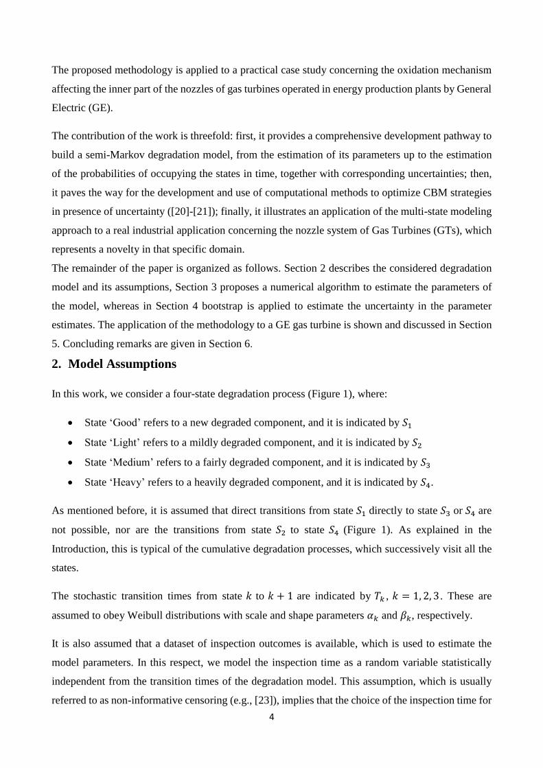
In this work, we consider a four-state degradation process (Figure 1), where:

State ‘Good’ refers to a new degraded component, and it is indicated by 𝑆1

State ‘Light’ refers to a mildly degraded component, and it is indicated by 𝑆2

State ‘Medium’ refers to a fairly degraded component, and it is indicated by 𝑆3

State ‘Heavy’ refers to a heavily degraded component, and it is indicated by 𝑆4.

As mentioned before, it is assumed that direct transitions from state 𝑆1 directly to state 𝑆3 or 𝑆4 are

not possible, nor are the transitions from state 𝑆2 to state 𝑆4 (Figure 1). As explained in the

Introduction, this is typical of the cumulative degradation processes, which successively visit all the

states.

The stochastic transition times from state 𝑘 to 𝑘 + 1 are indicated by 𝑇𝑘 , 𝑘 = 1, 2, 3 . These are

assumed to obey Weibull distributions with scale and shape parameters 𝛼𝑘 and 𝛽𝑘, respectively.

It is also assumed that a dataset of inspection outcomes is available, which is used to estimate the

model parameters. In this respect, we model the inspection time as a random variable statistically

independent from the transition times of the degradation model. This assumption, which is usually

referred to as non-informative censoring (e.g., [23]), implies that the choice of the inspection time for

5

each component in the dataset is not influenced by any information collected during the component

life (ongoing detections, measurements, etc.), which could have revealed, directly or indirectly, the

evolution of its degradation state. The justification of such an assumption again relates to the specific,

real case study considered in this paper (for further details, see [24]).

Figure 1: Scheme of the degradation mechanism

We assume that N inspections are conducted during the study period and 𝑛 components are inspected

each time. The i-th inspection outcome reports the degradation states of these 𝑛 components, which

have behaved independently of each other. Thus, the available dataset of inspection outcomes is made

up of N records, each one containing (Table 1):

1. The time at which the system has been inspected.

2. The number of components found in state 𝑆𝑠, (𝑖. 𝑒. , 𝑛𝑠) 𝑠 = 1, … ,4, where 𝑛 = ∑ 𝑛𝑠4𝑠=1 .

Finally, we assume that upon inspection, the n-components system is removed from operation, to be

submitted to the proper repair actions, which depend on the degradation states of the individual

components. These actions are assumed to always bring the system back to an As Good As New

(AGAN) state. This assumption is made because of its direct relation to the specific, real case study

considered in this work, which concerns modular GTs: when a GT module is removed, it is sent back

to the workshop to undergo a maintenance overhaul, while an AGAN module replaces it on the GT.

Table 1: example of Part Life Data Base (n=22)

Record Time inspec. 𝑛1 𝑛2 𝑛3 𝑛4

1 130 4 5 9 4

2 180 0 10 11 1

… … … … …

N 200 15 5 1 1

In this context, the aim of this work is to:

Light Medium Heavy Good

6

- Apply the MLE technique on the available dataset to infer the values of the parameters of the

four-state degradation model.

- Implement a technique to estimate the FIM, which is then used to estimate the confidence

intervals on the estimated semi-Markov model parameters.

- Implement a technique for propagating the estimated uncertainties (confidence intervals) onto

the probabilities of occupying the degradation states over time. This allows estimating the

component future failure behavior and support the business department in the estimation of the

costs of maintenance service contracts to be offered to the customers.

3. Parameter Estimation

The aim of this section is to determine the analytical expression of the likelihood function 𝐿(𝑻; 𝜽),

where the vector 𝑻 contains the three stochastic transition times 𝑇𝑘, 𝑘 = 1,… , 3 we are interested in.

To do this, we need to compute the probability of finding the component in state 𝑆1 at inspection

time 𝑡𝑖 , 𝑖 = 1,… ,𝑁, which is defined as:

𝑃1𝑖 = 𝑅1(𝑡𝑖; 𝛼1, 𝛽1 ) = 𝑃(𝑇1 > 𝑡𝑖; 𝛼1, 𝛽1) (1)

Where 𝑅1(𝑡𝑖; 𝛼1, 𝛽1 ) is the Complementary Cumulative Distribution Function (CCDF, also referred

to as survival function) of the transition time 𝑇1, whose parameters are 𝛼1, 𝛽1 .

The probability 𝑃2𝑖 of finding the component in state 𝑆2 at inspection time 𝑡𝑖 is given by:

𝑃2𝑖 = ∫ 𝑓1(𝜏)𝑅2( 𝑡𝑖 − 𝜏; 𝛼2, 𝛽2 )𝑑𝜏

𝑡𝑖0

(2)

where 𝑓1( 𝑡) represents the probability density function (pdf) of the transition time 𝑇1 from state 𝑆1

‘Good’ to state 𝑆2 ‘Light’, whereas 𝑅2( 𝑡𝑖; 𝛼2, 𝛽2 ) is the CCDF of the transition time 𝑇2 , with

parameters 𝛼2, 𝛽2.

The probability 𝑃3𝑖 of finding the component in state 𝑆3 ‘Medium’ at inspection at time 𝑡𝑖 reads:

𝑃3𝑖 = ∫ ∫ 𝑓1(𝜏1)𝑓2(𝜏2 − 𝜏1)𝑅3( 𝑡𝑖 − 𝜏2; 𝛼3, 𝛽3 )𝑑𝜏2𝑑𝜏1

𝑡𝑖𝜏1

𝑡𝑖0

(3)

where 𝑓2( 𝑡) represents the pdf of 𝑇2, whereas 𝑅3( 𝑡𝑖; 𝛼3, 𝛽3 ) is the CCDF of the transition time 𝑇3,

with parameters 𝛼3, 𝛽3.

Finally, the probability 𝑃4𝑖 of finding the component in state Heavy at inspection is derived from the

constraint that the four probability values 𝑃𝑠𝑖, 𝑠 =1,…, 4 must sum to one:

𝑃4𝑖 = 1 − 𝑃1

𝑖 − 𝑃2𝑖 − 𝑃3

𝑖 (4)

7

The parameter estimation problem considered in this work is concerned to inferring the values

(𝛼𝑘, 𝛽𝑘) of the scale and shape parameters, respectively, of the Weibull distribute transition time 𝑇𝑘

from state 𝑆𝑘 to state 𝑆𝑘+1, 𝑘 = 1, 2, 3. These parameters are arranged in the vector 𝜽 =

(𝛼1, 𝛽1 , 𝛼2, 𝛽2, 𝛼3, 𝛽3).

The likelihood function is multinomial distribution, which reads:

𝐿(𝑻; 𝜽) = ∏𝑛!

𝑛1𝑖 !𝑛2

𝑖 !𝑛3𝑖 !(1−𝑛1

𝑖−𝑛2𝑖−𝑛3

𝑖 )!

𝑁𝑖=1 (𝑃1

𝑖)𝑛1𝑖(𝑃2𝑖)𝑛2

𝑖(𝑃3𝑖)𝑛3

𝑖(1 − 𝑃1

𝑖 − 𝑃2𝑖 − 𝑃3

𝑖)𝑛−𝑛1𝑖−𝑛2

𝑖−𝑛3𝑖 (5)

where

𝑛𝑠𝑖 represents the number of components in state 𝑆𝑠 at inspection time 𝑡𝑖, 𝑠 =

1, … . , 4, 𝑖 = 1,… ,𝑁.

𝑛 is the total number of components in the same turbine inspected at each time.

Finally, as usual [18], instead of the likelihood function L(𝑻; 𝜽), one can maximize the log-likelihood

function l(𝑻; 𝜽), which is its natural logarithm. In fact, l(𝑻; 𝜽) tends to be simpler than L(𝑻; 𝜽), as

when we take logs, products are changed to sums.

The analytical solution of such MLE problem is impracticable, because the log-likelihood function is

made up of convolution integrals, for which there is no solution in closed form. Thus, we first use the

adaptive quadrature method ([22]) to numerically calculate the integrals in Eqs (2-3). Then, a

combination of optimization algorithms available in the MATLAB Global Optimization toolbox

([25]-[28]) is used to find the maximum of the log-likelihood function. In this respect, notice that the

search space in which the optimization algorithm is asked to find the maximum value of the log-

likelihood function is very large, as it has M=6 dimensions, and there may be local maxima and flat

regions. Thus, it may happen that after running any of the optimization algorithms contained in the

toolbox (i.e., genetic algorithms, active set method, Nelder-Mead simplex algorithm, etc. [25]-[28])

with a large number of iterations, we get an incorrect ML estimate (a local minimum), or even a Not

a Number.

The strategy proposed to overcome this problem is to successively run, for a relatively large number

of times (e.g., 5 times), different optimization algorithms. That is, an optimization algorithm is

initially run, which provides a first solution in the 6D solution space. Then, each of these 6 entries is

multiplied by a number randomly sampled from {0.75, 1.25} (i.e., 25% more or less than the proposed

solution). This new, modified point, not far from the starting point, indicates the region of the search

space where the MLE values have to be sought, and it is the starting point from which the next,

possibly different, optimization algorithm begins the search we take as final optimum point the one

8

indicated as optimum by the majority of the algorithm runs. The repeated application of different

optimization algorithms starting from different points is done to reduce the risk of finding a local

maximum (future research work will focus on the potential use of the ensemble of optimization

algorithms for searching the log-likelihood global maximum).

4. Confidence Intervals

To estimate the uncertainty in the MLE values, we exploit the asymptotic properties of the ML

estimator, which hold under mild regularity conditions [18], [30]. That is, if �̂� = (𝜃1, … . , 𝜃𝑀), with

𝑀 ≥ 1 number of parameters to be estimated, is a unique solution to the maximization problem of

𝑙(𝑇; 𝜽), then:

1) E(�̂�) → 𝜽

2) �̂� �̂� = (�̂�𝜽𝟏 , … . . , �̂�𝜽𝑴) → (�̂�𝜽𝟏 , … . . , �̂�𝜽𝑴)𝑪𝑹 (6)

where (�̂�𝜽𝟏 , … . . , �̂�𝜽𝑴)𝑪𝑹 is the Cramer-Rao lower bound of the standard deviations of any

unbiased estimator of 𝜽 [18]. That is, any choice of an unbiased estimator of 𝜽 brings a

variability in �̂� necessarily larger than �̂�𝑪𝑹.

3) �̂� is asymptotically normal; that is, �̂� − 𝜽~𝑁(0, 𝑭−1(�̂�)).

where 𝑭(�̂�) is the expected FIM calculated at the MLE point. The generic (𝑚, 𝑗) entry of 𝑭(𝜽), 𝑚,

𝑗 = 1, . . . . , 𝑀, is:

𝐹𝑚𝑗 = 𝐸 [ 𝜕𝑙(𝑻; 𝜽)

𝜕𝜗𝑚∙𝜕𝑙(𝑻; 𝜽)

𝜕𝜗𝑗 ] (7)

Under mild regularity conditions, FIM is equal to the average of the Hessian of 𝑙(𝑻; 𝜽):

−

(

𝐸 [

𝜕2𝑙(𝑻; 𝜽)

𝜕𝜗12 ] ⋯ 𝐸 [

𝜕2𝑙(𝑻; 𝜽)

𝜕𝜗1𝜕𝜗𝑀 ]

⋮ ⋱ ⋮

𝐸 [ 𝜕2𝑙(𝑻; 𝜽)

𝜕𝜗𝑀𝜕𝜗1 ] ⋯ 𝐸 [

𝜕2𝑙(𝑻; 𝜽)

𝜕𝜗𝑀2 ])

(8)

Notice that the second derivatives give a measure of how quickly the log-likelihood changes when

we change the parameter values in the proximity of the ML estimate. Then, if the Fisher information

is large, the distribution changes quickly when we move from the MLE value of the parameter. This

entails that we should be able to properly estimate �̂� based on the data. On the other hand, if Fisher

9

information is small, this means that the distribution is ’very similar’ to distributions with parameter

not so close to �̂� and, thus, more difficult to distinguish; thus, our estimation will be worse.

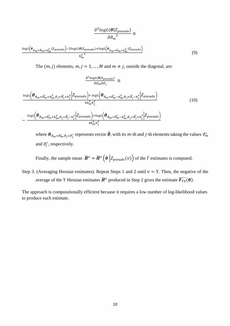
However, the computation of the FIM in the present case study is even more difficult than that of the

MLE, as it requires computing the derivatives of 𝑙(𝑻; 𝜽), for which analytical solutions are not

practicable. Thus, the computer resampling approach proposed in [29] is considered in this work to

estimate 𝑭(𝜽), which uses a computationally efficient and easy-to-implement method for Hessian

estimation.

The underlying idea of the method is to produce a large number of Simultaneous Perturbation (SP)

estimates of the Hessian matrix of 𝑙(𝑻; 𝜽) and, then, average the negative of these estimates to obtain

an approximation to 𝑭(𝜽) (Figure 2).

The algorithm is presented in detail below:

Step 0. (Initialization). Set the number Υ of pseudo-data vectors that will be generated, and inizialize

𝑣=1.

Step 1. (Generating pseudo-data). Based on the ML Estimate �̂�, generate the 𝑣-th pseudo-dataset

𝑍𝑝𝑠𝑒𝑢𝑑𝑜(𝑣) of N records. Namely, to produce the SP Hessian estimates, we implement the

following procedure to generate a dataset similar to the original:

1. Set i=1.

2. Consider the inspection time of the i-th record in the available dataset.

3. Simulate the histories of the n components in the i-th record, assuming that the parameters of

the stochastic process take their ML estimate �̂�.

4. Store the outcomes.

5. i=i+1.

6. Repeat steps 2-4 until i >N.

Step 2. (Hessian estimation): With the 𝑣-th pseudo-data vector in Step 1, compute the Γ Hessian

estimates �̂�𝛾, 𝛾 = 1… , Γ . To do this, we first build the perturbation vector ℎ𝛾 =

(ℎ1𝛾, … . , ℎ𝑀

𝛾), whose elements are uniformly distributed zero-mean random variables with

bounds satisfying the condition 𝐸 [|1

ℎ𝑚𝛾 |] < ∞, 𝑚 = 1,… ,𝑀 . Then, we use the finite

difference method [31] for estimating the second derivatives. In particular, the m-th element

on the diagonal of �̂�𝛾 is:

10

𝜕2𝑙𝑜𝑔𝐿(𝜽|𝑍𝑝𝑠𝑒𝑢𝑑𝑜)

𝜕𝜗𝑚2 ≅

𝑙𝑜𝑔𝐿(𝜽𝜗𝑚=�̂�𝑚+ℎ𝑚

𝛾 |𝑍𝑝𝑠𝑒𝑢𝑑𝑜)−2𝑙𝑜𝑔𝐿(𝜽|𝑍𝑝𝑠𝑒𝑢𝑑𝑜)+𝑙𝑜𝑔𝐿(𝜽𝜗𝑚=�̂�𝑚+ℎ𝑚𝛾 |𝑍𝑝𝑠𝑒𝑢𝑑𝑜)

ℎ𝑚𝛾 2

(9)

The (𝑚, 𝑗) elements, 𝑚, 𝑗 = 1,… ,𝑀 and 𝑚 ≠ 𝑗, outside the diagonal, are:

𝜕2𝑙𝑜𝑔𝐿(𝜽|𝑍𝑝𝑠𝑒𝑢𝑑𝑜)

𝜕𝜗𝑚𝜕𝜗𝑗 ≅

𝑙𝑜𝑔𝐿(𝜽𝜗𝑚=𝜗�̂�+ℎ𝑚

𝛾,𝜗𝑗=𝜗�̂�+ℎ𝑗

𝛾|𝑍𝑝𝑠𝑒𝑢𝑑𝑜)+ 𝑙𝑜𝑔𝐿(𝜽𝜗𝑚=𝜗�̂�−ℎ𝑚𝛾,𝜗𝑗=𝜗�̂�−ℎ𝑗

𝛾|𝑍𝑝𝑠𝑒𝑢𝑑𝑜)

4ℎ𝑚𝛾ℎ𝑗𝛾 (10)

− 𝑙𝑜𝑔𝐿(𝜽𝜗𝑚=𝜗�̂�+ℎ𝑚

𝛾,𝜗𝑗=𝜗�̂�−ℎ𝑗

𝛾|𝑍𝑝𝑠𝑒𝑢𝑑𝑜)+𝑙𝑜𝑔𝐿(𝜽𝜗𝑚=𝜗�̂�−ℎ𝑚𝛾,𝜗𝑗=𝜗�̂�+ℎ𝑗

𝛾|𝑍𝑝𝑠𝑒𝑢𝑑𝑜)

4ℎ𝑚𝛾ℎ𝑗𝛾

where 𝜽𝜗𝑚=𝜗𝑚∗ ,𝜗𝑗=𝜗𝑗∗ represents vector �̂�, with its 𝑚-th and 𝑗-th elements taking the values 𝜗𝑚

∗

and 𝜗𝑗∗, respectively.

Finally, the sample mean �̅�𝑣 = �̅�𝑣 (𝜽 |𝑍𝑝𝑠𝑒𝑢𝑑𝑜(𝑣)) of the Γ estimates is computed.

Step 3. (Averaging Hessian estimates). Repeat Steps 1 and 2 until 𝑣 = Υ. Then, the negative of the

average of the Υ Hessian estimates �̅�𝑣 produced in Step 2 gives the estimate 𝑭ΓΥ̅̅ ̅̅ ̅(𝜽).

The approach is computationally efficient because it requires a low number of log-likelihood values

to produce each estimate.

11

Figure 2: Synoptic of the overall procedure and, in particular, of the bootstrap approach to estimate the Fisher

Information Matrix

4.1. Construction of the confidence intervals

Approximate confidence intervals for the model parameters can be obtained by using the asymptotic

property of the MLE estimators, that is the distribution is normal with means equal to the MLE values

and covariance matrix equal to the inverse of the FIM [18].

Dataset

Loglikelihood Calculation

Pseudo data input

Hessian estimates �̂�𝛾 �̅�𝛾(𝜐)

= average of �̂�𝛾

𝑍𝑝𝑠𝑒𝑢𝑑𝑜(𝜐 = 1)

𝑍𝑝𝑠𝑒𝑢𝑑𝑜(𝜐 = 2)

𝑍𝑝𝑠𝑒𝑢𝑑𝑜(𝜐 = Υ)

…

�̂�1, �̂�2,…, �̂�Γ

�̂�1, �̂�2,…, �̂�Γ

�̂�1, �̂�2,…, �̂�Γ

…

�̅�1

�̅�2

�̅�Υ

Ne

gative average of 𝐻

(𝜐)

Information Matrix Estimate

�̅�ΓΥ

Uncertainty estimation

ML-Estimation

Monte-Carlo Propagation

12

On this basis, an approximate 100(1 − 𝛼)% normal-theory, Wald confidence region for �̂� is the set

of all the 𝜽 in the ellipsoid ([32], [33]):

(�̂� − 𝜽) ∙ 𝑭−𝟏(�̂�) ∙ (�̂� − 𝜽)′ ≤ 𝝌𝟐(1 − 𝛼,𝑀) (11)

where 𝝌𝟐(1 − 𝛼,𝑀) is the (1 − 𝛼)𝑡ℎ quantile of the chi-square distribution with 𝑀 degrees of

freedom, and 𝑀 is the number of parameters (i.e., 𝑀 = 6 in the considered case study).

On the other hand, for a positive definite parameter (e.g., one of the parameters of the Weibull

distribution), the normal approximation is sometimes unsatisfactory because the distribution centred

in the MLE values may have the tails in the negative parts of the hyper-space, thus giving negative

lower bounds of the confidence intervals. In this case, the delta method [34] is adopted, which

improves the quality of the approximation by applying a suitable re-parameterization of the

parameters (i.e., a transformation of the parameters to a new scale). The algorithm is presented in

detail below.

The delta method states that we can work, instead of 𝜽, with a differentiable non-zero valued function

𝜙(𝜽), which is again asymptotically normally distributed around 𝜙(�̂�), with adjusted variance value

σ̂2{𝜙(�̂�)} = 𝜙′(�̂�)𝑇𝑭−𝟏(�̂�)𝜙′(�̂�), where 𝜙′(�̂�) is the diagonal matrix of the partial derivatives of 𝜙

with respect to the parameters in 𝜽, calculated in �̂�. That is:

𝜙(𝜽) ~𝑁(𝜙(�̂�), 𝜙′(�̂�)𝑭−𝟏(�̂�)𝜙′(�̂�)𝑇) (12)

In this work we consider the function identity for the parameters with positive distribution whereas,

in according to [33], 𝜙(∙) = ln(∙) for those parameters with negative tails.

5. Case Study

GE offers to its customers a maintenance service on GTs. This service include maintaining the nozzles

of the GTs, which are affected by high-temperature oxidation. This mechanism occurs when nickel-

based super alloys are exposed to temperatures higher than 538°C. Oxygen in the gas stream reacts

with the nickel alloy to form a nickel-oxide layer on the airfoil surface. When subjected to vibration

and start-stop thermal cycles during operation, this nickel oxide layer tends to crack and spall. This

phenomenon may also occur on the inner surfaces of blade cooling passages and result in blade failure

[12].

13

When nozzles are removed from the turbine system upon a scheduled or opportunistic maintenance

action, they are delivered to the GE workshop. There, GE experts check the component and classify

its health state into ‘Good’, ‘Light’, ‘Medium’ and ‘Heavy’ ordinal categories, by comparing the

amount of degradation (i.e., the oxidized area) with three thresholds Tg, Tl, Tm:

If the oxidized area is smaller than Tg, then the nozzle is not maintained.

If the oxidized area indicator is larger than Tm, then the component is replaced.

If the oxidized area is between Tg and Tl, then a maintenance action based on brazing is

performed.

If the oxidized area is between Tl and Tm, then a welding repair action is performed.

Depending on the degradation state, different workshop activities are carried out to send back to the

customer the nozzle system in an As Good As New (AGAN), or even new, state.

A number of physical models have been proposed to describe the behaviour of the oxidation

mechanism, which emphasize the dependence of the degradation evolution on the type of substance

that creates oxidation ([37], [38]). This information is at the basis of the development of the proposed

multi-state degradation model, to describe the dynamics of stochastic transition among the 4

degradation states identified by the maintenance operators. Given the cumulative, incremental nature

of the degradation process under study, we assume that the transitions in the model can occur from

one degradation state to the next degraded state, only, and, as mentioned before, at Weibull-

distributed stochastic time instants.

The information about the nozzle system operating life and the result of the workshop classification

are stored in a Part Life Data Base (PLDB) for reliability life data analysis. In particular, with regards

to the oxidation mechanism, the PLDB contains a set of 𝑁 = 30 records of field observations of the

nozzle systems of turbines operated by GE. We anticipate that the data considered in this paper came

from real GE field experience, but they have been re-scaled in arbitrary time units to respect the GE

policy on confidential information.

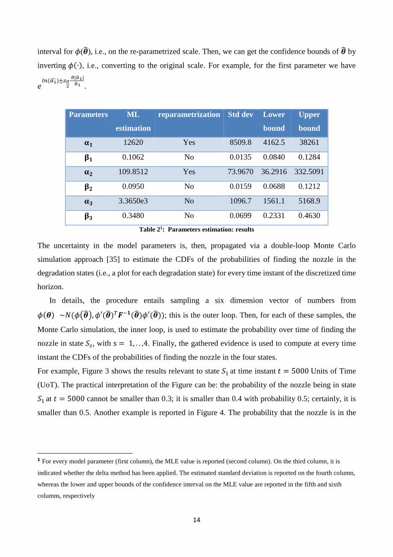
Table 2 reports the ML estimate of 𝜽 (second column) and the parameters on which the delta method

has been applied (third column). That is, in this case study 𝜙(𝜽) = [ ln(α1), β1, ln(α2), β2, 𝛼3, β3],

and the diagonal of 𝜙′ is 𝑑𝑖𝑎𝑔(𝜙′(𝜽)) = [ 1/α1, 1, 1/α2, 1, 1, 1]. The fourth column gives the value

of the standard deviations, which are the square roots of the elements of the diagonal of 𝑭−𝟏(�̂�).

Finally, the last two columns show the 90% confidence bounds of �̂�. To find these values, we have

used the common formula 𝜙(�̂�) ± 𝑧𝛼2∙ σ̂{𝜙(�̂�)}, for estimating the equal-tails 1 − 𝛼 confidence

14

interval for 𝜙(�̂�), i.e., on the re-parametrized scale. Then, we can get the confidence bounds of �̂� by

inverting 𝜙(∙), i.e., converting to the original scale. For example, for the first parameter we have

𝑒𝑙𝑛(α1̂)±𝑧𝛼

2∙σ̂{α̂1}

α̂1 .

Parameters ML

estimation

reparametrization Std dev Lower

bound

Upper

bound

𝛂𝟏 12620 Yes 8509.8 4162.5 38261

𝛃𝟏 0.1062 No 0.0135 0.0840 0.1284

𝛂𝟐 109.8512 Yes 73.9670 36.2916 332.5091

𝛃𝟐 0.0950 No 0.0159 0.0688 0.1212

𝛂𝟑 3.3650e3 No 1096.7 1561.1 5168.9

𝛃𝟑 0.3480 No 0.0699 0.2331 0.4630

Table 21: Parameters estimation: results

The uncertainty in the model parameters is, then, propagated via a double-loop Monte Carlo

simulation approach [35] to estimate the CDFs of the probabilities of finding the nozzle in the

degradation states (i.e., a plot for each degradation state) for every time instant of the discretized time

horizon.

In details, the procedure entails sampling a six dimension vector of numbers from

𝜙(𝜽) ~𝑁(𝜙(�̂�), 𝜙′(�̂�)𝑇𝑭−𝟏(�̂�)𝜙′(�̂�)); this is the outer loop. Then, for each of these samples, the

Monte Carlo simulation, the inner loop, is used to estimate the probability over time of finding the

nozzle in state 𝑆𝑠, with s = 1, . . ,4. Finally, the gathered evidence is used to compute at every time

instant the CDFs of the probabilities of finding the nozzle in the four states.

For example, Figure 3 shows the results relevant to state 𝑆1 at time instant 𝑡 = 5000 Units of Time

(UoT). The practical interpretation of the Figure can be: the probability of the nozzle being in state

𝑆1 at 𝑡 = 5000 cannot be smaller than 0.3; it is smaller than 0.4 with probability 0.5; certainly, it is

smaller than 0.5. Another example is reported in Figure 4. The probability that the nozzle is in the

1 For every model parameter (first column), the MLE value is reported (second column). On the third column, it is

indicated whether the delta method has been applied. The estimated standard deviation is reported on the fourth column,

whereas the lower and upper bounds of the confidence interval on the MLE value are reported in the fifth and sixth

columns, respectively

15

fourth state at time 𝑡 = 5000 UoT is smaller or equal to 0.46 with probability almost 1. Similar plots

are produced for 𝑆2 and 𝑆3 .

Figure 3: CDF of the probability of state 𝑺𝟏 at t=5000 UoT

Figure 4: CDF of the probability of state S4 at t=5000 UoT

Figure 4 shows the link between the CDF of the state probability at a given time instant and the time-

dependent state probability, with associated confidence interval.

16

Figure 5: Link between CDF of the state probability at a specific time instant and time-depended state

probability, with associated confidence interval of 90%. The extreme points of this interval (i.e., 5th and

95th percentiles) are reported on the time axis.

Figure 6 shows the time-depended probability values of the nozzle being in the four degradation

states, which is useful information to make decisions. It emerges that:

In the initial part of the component life, the items are healthy, with probability of

finding the nozzle in state 1 at time 0 equal to 1.

In the successive time instants, the nozzle starts to increase the probability of

leaving state 𝑆1 to reach state 𝑆2; the first three plots in Figure 6 show that the

sojourn times in states 𝑆1 , 𝑆2 and 𝑆3 are on average very small, with a large

variance, due to the small values of the shape parameters.

As time goes on, the probability that the nozzle undergoes a transition from state

𝑆2 to state 𝑆3 does not significantly increase.

Finally, as the time evolves, the nozzle reaches the failure state.

From these considerations, it emerges that further practical work must be spent on investigating

whether the degradation mechanism should be modelled as a three-state system. In fact, the smaller

number of parameters to be estimated may provide parameter MLE affected by a small amount of

uncertainty. However, this investigation does not concern looking at the results that one would get if

two of the four states were merged together; rather, GE engineers should find two new threshold

values for the oxidized area, based on their physical knowledge of the degradation phenomenon: once

a PLDB with respect to these new threshold values is available, then a 3-state system model can be

developed.

17

Figure 6: Time-depended state probability, with associated confidence interval of 90%.

The output of the proposed procedure, summarized in Figure 6, can be exploited in approaches like

those developed by the authors to optimize CBM strategies ([20], [21]) based on multi-state models

of degradation, with uncertain parameters. In particular, two techniques based on Multi Objective

Genetic Algorithms have been proposed in [21] to solve the problem of the optimal inspection

scheduling within a CBM strategy. Both techniques rely on an innovative algorithm for sorting

probability distributions and on a new definition of Pareto dominance. The first technique is based

on the NSGA-II algorithm, whereas the second is a combination of NSGA-II and the CVaR index.

Yet, a similar solution has been proposed in [20], where the uncertainty is handled within the

framework of the Dempster-Shafer theory of evidence. From these studies, it also emerges the added

value of giving due account to uncertainty when making maintenance decisions: it gives the

18

possibility of choosing maintenance settings which would be otherwise discarded if the decision

maker looks at the expected values only.

6. Conclusion

In this paper, a methodology to build a four-state semi-Markov model of degradation has been

developed. In particular, the methodology proposed allows estimating the model parameters,

characterizing the related uncertainty and propagating it onto the probabilities of occupying the

different states over time.

This output has paved the way for the development of advanced computational techniques to optimize

maintenance policies in the presence of uncertainty and imprecisions.

A practical case study has been considered, which concerns the oxidation degradation mechanism

that affects the nozzles of gas turbines. The case study has shown the potential of the method and, at

the same time, has uncovered the practical possibility of describing the degradation process in three

states.

Future research work will focus on the development of Bayesian methods for estimating the

parameters of the multi-state degradation model.

7. Reference

[1]. Baraldi, P., Balestrero, A., Compare, M., Benetrix, L., Despujols, A., Zio, E., “A modeling

framework for maintenance optimization of electrical components based on fuzzy logic and

effective age”, Quality and Reliability Engineering International. Vol. 29, No. 3, pp. 385-405,

2013.

[2]. Baraldi, P., Compare, M., Zio, E., “Uncertainty analysis in degradation modeling for

maintenance policy assessment”, Proceedings of the Institution of Mechanical Engineers, Part

O: Journal of Risk and Reliability, Vol. 227, No. 3, pp. 267-278, 2013.

[3]. Baraldi P., Compare, M., Zio, E., “Maintenance policy performance assessment in presence

of imprecision based on Dempster–Shafer Theory of Evidence”, Information Sciences. Vol.

245, pp. 112-131, 2013.

[4]. Baraldi, P., Compare, M., Zio, E., “A practical analysis of the degradation of a nuclear

component with field data, in Reliability and Risk analysis: Beyond the Horizon”, Eds.

R.D.J.M. Steenbergen, P.H.A.J.M. van Gelder, S. Miraglia, A.C.W.M. Vrouwenvelder, CRC

Press, 2013.

[5]. Baraldi, P., Compare, M., Despujols, A., Zio, E., “Modelling the effects of maintenance on

the degradation of a water-feeding turbo-pump of a nuclear power plant”, Proceedings of the

19

Institution of Mechanical Engineers, Part O: Journal of Risk and Reliability, Vol. 225, No. 2,

pp. 169-183, 2011.

[6]. Moghaddass, R., Zuo, M.J., “A parameter estimation method for a multi-state deteriorating

system with incomplete information”, Proceeding of the Seventh International Conference on

Mathematical Methods in Reliability: Theory, Methods, and Applications (MMR 2011), pp.

34-42, 2011.

[7]. Moghaddass, R., Zuo, M.J., “Multi-state degradation analysis for a condition monitored

device with unobservable states”, Proceedings of 2012 International Conference on Quality,

Reliability, Risk, Maintenance, and Safety Engineering, ICQR2MSE 2012, pp. 549-554,

2012.

[8]. Levitin, G., Lisnianski, A., Ushakov I. “Reliability of Multi-State Systems: A Historical

Overview,” Mathematical and statistical methods in reliability, Lindqvist, Doksum (eds.),

World Scientific, pp. 123-137, 2003.

[9]. Zuo, M. J., Huang, J. and Kuo, W. "Multi-state k-out-of-n Systems," Reliability Engineering

Handbook, (H. Pham, ed.), Springer-Verlag, London, September 2001.

[10]. Vrignat, P., Avila, M., Duculty, F., Aupetit, S., Slimane, M., Kratz, F. “Maintenance

policy: degradation laws versus Hidden Markov Model availability indicator,” Proceedings

of the Institution of Mechanical Engineers, Part O: Journal of Risk and Reliability Vol. 226,

No. 2, pp. 137-155, 2011.

[11]. Lisnianski, A., Levitin, G. “Multi-State System Reliability: Assessment, Optimization

and Applications,” Series on Quality, Reliability and Engineering Statistics: Volume 6, World

Scientific, 2003.

[12]. Greenfield, P., “Creep of Metals at High Temperatures,” M&B Monograph ME/9,

Mills and Boon Ltd., London, England, 1972.

[13]. Fleming, K.N., “Markov models for evaluating risk-informed in-service inspection

strategies for nuclear power plant piping systems,” Reliability Engineering and System

Safety, Vol. 83, No. 1, pp. 27-45 2004.

[14]. Di Maio, F., Colli, D., Zio, E., Tong, J., “A multi-state Approach for the Reliability

Assessment of Nuclear Power Plants Piping Systems, submitted for publication.

[15]. Zio, E., Compare, M., “Evaluating maintenance policies by quantitative modeling and

analysis”, Reliability Engineering and System Safety, Vol. 109, pp. 53-65, 2013.

[16]. Zio, E., Compare, M., “A snapshot on maintenance modeling and applications. Marine

Technology and Engineering”, Vol. 2, pp. 1413-1425, 2013.

20

[17]. Zio, E., “Computational Methods for Reliability and Risk Analysis”, World Scientific

Publishing, Singapore, 2009.

[18]. Papoulis, A. And Pillai S.U. 2002. “Probability, Random Variables and Stochastic

Processes”, 4th edition, International Edition, Mc-Graw-Hill.

[19]. Efron B., Tibshirani R.J. “An introduction to the bootstrap”, Chapman & Hall, New

York, 1993.

[20]. Compare, M., Zio, E., “Genetic algorithms in the framework of Dempster-Shafer

theory of evidence for maintenance optimization problems,” IEEE Transactions on

Reliability, Vol. 64, No. 2, pp. 645-660, 2015.

[21]. Compare, M., Martini, F., Zio, E., “Genetic algorithms for condition-based

maintenance optimization under uncertainty,” European Journal of Operational Research,

Vol. 244, No. 2, pp. 611-623, 2015.

[22]. Gander, W. and W. Gautschi, “Adaptive Quadrature – Revisited,” BIT, Vol. 40, pp.

84-101, 2000.

[23]. Christensen, R., Johnson, W., Branscum, A., Hanson, T., “Bayesian Ideas and Data

Analysis: An Introduction for Scientists and Statisticians,” CRC Press, 2010.

[24]. Di Maio, F., Compare, M., Mattafirri, S., Zio, E. “A double-loop Monte Carlo

approach for Part Life Data Base reconstruction and scheduled maintenance improvement,”

Safety and Reliability: Methodology and Applications - Proceedings of the European Safety

and Reliability Conference, ESREL 2014, pp. 1877-1884, 2015.

[25]. Lagarias, J.C., Reeds, J. A., Wright, M. H., Wright, P.E., “Convergence Properties of

the Nelder-Mead Simplex Method in Low Dimensions,” SIAM Journal of Optimization, Vol.

9, No. 1, pp. 112-147, 1998.

[26]. Powell, M.J.D., “A Fast Algorithm for Nonlinearly Constrained Optimization

Calculations,” Numerical Analysis, ed. G.A. Watson, Lecture Notes in Mathematics,

Springer-Verlag, Vol. 630, 1978.

[27]. Powell, M.J.D., “The Convergence of Variable Metric Methods For Nonlinearly

Constrained Optimization Calculations,” Nonlinear Programming 3 (Mangasarian, Meyer,

and Robinson, eds.), Academic Press, 1978.

[28]. Waltz, R.A., Morales, J.L., Nocedal, J., Orban, D., “An interior algorithm for nonlinear

optimization that combines line search and trust region steps,” Mathematical Programming,

Vol. 107, No. 3, pp. 391–408, 2006.

21

[29]. Spall, J.C. “Monte Carlo Computation of the Fisher Information Matrix in

Nonstandard Settings”, Journal of Computational and Graphical Statistics, Vol. 14, No. 4, pp.

889–909, 2005.

[30]. Kendall, M. and Stuart A., “The Advanced Theory of Statistics,” Vol. 2, Charles

Griffin and Company limited, London & High Wycombe, 1979

[31]. Quarteroni, A. “Modellistica Numerica per Problemi Differenziali”, 4th Edition,

Springer 2008.

[32]. Cox, D.R., Hinkley, D. V., “Theoretical Statistics”, Chapman and Hall, London, 1974.

[33]. Meeker, W.Q., Escobar, L.A., “Teaching About Approximate Confidence Regions

Based on Maximum Likelihood Estimation”, The American Statistician, Vol. 49, No. 1, pp.

48-53, 1995.

[34]. Giorgio, M., Guida, M., Pulcini, G., “An age- and state-dependent Markov model for

degradation processes”, IIE Transactions, Vol. 43, No. 9, pp. 621-632, 2011.

[35]. Zio, E., “The Monte Carlo Simulation Method for System Reliability and Risk

Analysis”, Springer, 2013.

[36]. Zio, E., “An introduction to the basics of reliability and risk analysis”, WorldScientific

Publishing Company, Singapore, 2007.

[37]. Wood, I.H., Foster, A.D., Schilke, P.W., “High Temperature Coating for Improved

Oxidation/Corrosion Protection," GE Turbine Reference Library Publication GER 3597,

1990.

[38]. Kurz, R., Brun, K., “Degradation in Gas Turbine System”, The American Society Of

Mechanical Engineers, ASME paper 2000-GT-345.