56
Semi-Supervised Learning in Gigantic Image Collections Rob Fergus (New York University) Yair Weiss (Hebrew University) Antonio Torralba (MIT)
| Date post: | 10-Dec-2015 |
| Category: |
Documents |
| Upload: | gavin-newman |
| View: | 215 times |
| Download: | 0 times |
Semi-Supervised Learning in Gigantic Image Collections
Rob Fergus (New York University)
Yair Weiss (Hebrew University)Antonio Torralba (MIT)
What does the world look like?
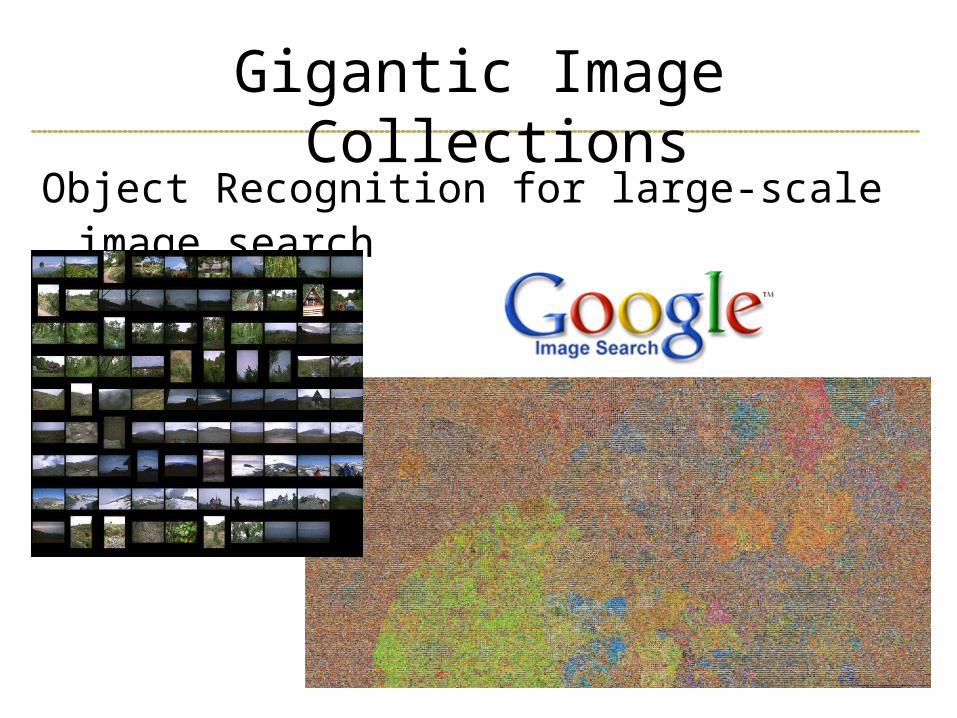
High level image statisticsObject Recognition for large-scale image search
Gigantic Image Collections
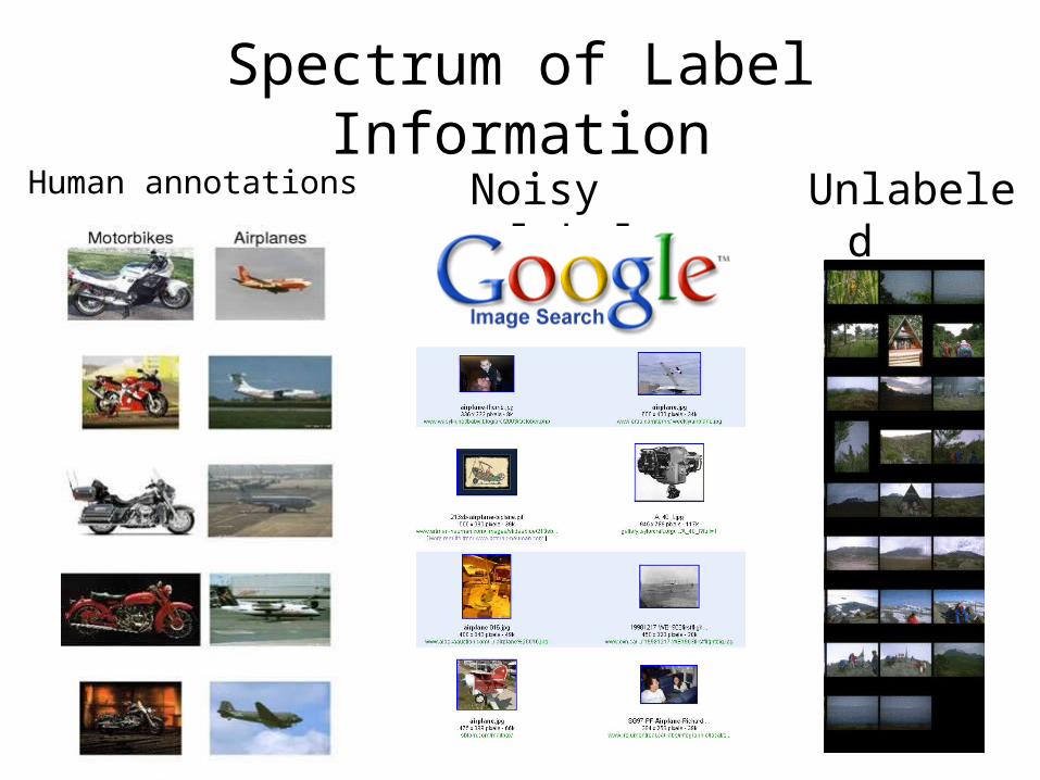
Spectrum of Label InformationHuman annotations Noisy
labelsUnlabele
d
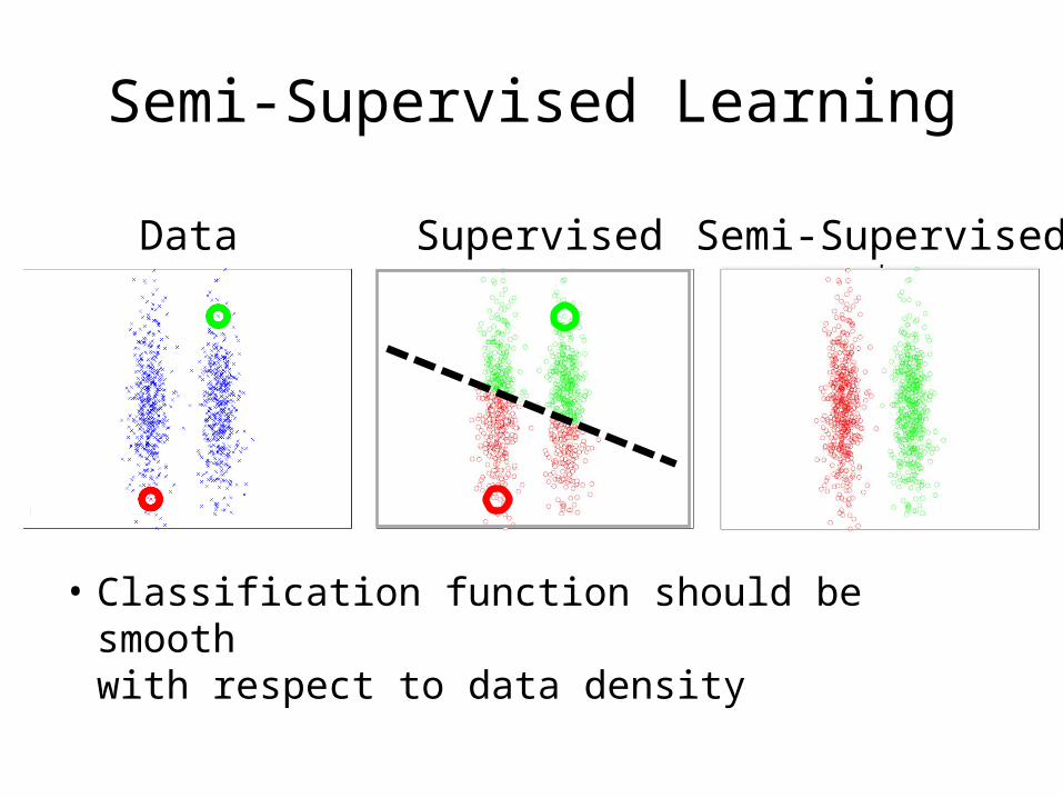
Semi-Supervised Learning
• Classification function should be smooth with respect to data density
Data Supervised Semi-Supervised
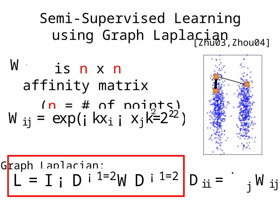
Semi-Supervised Learning using Graph Laplacian
is n x n affinity matrix (n = # of points)
Wi j = exp(¡ kxi ¡ xj k=2²2)
Di i =P
j Wi jL = D ¡ 1=2LD ¡ 1=2 = I ¡ D ¡ 1=2WD ¡ 1=2Graph Laplacian:
[Zhu03,Zhou04]
Wi j = exp(¡ kxi ¡ xj k=2²2)
L = D ¡ 1=2LD ¡ 1=2 = I ¡ D ¡ 1=2WD ¡ 1=2
Wi j = exp(¡ kxi ¡ xj k=2²2)
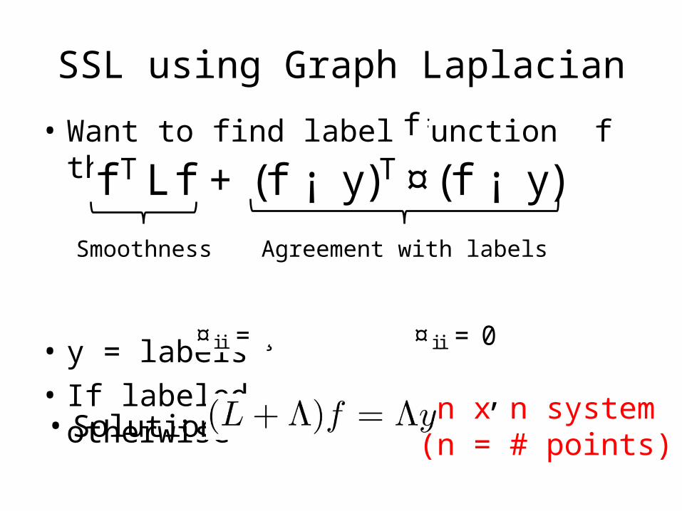
• Want to find label function f that minimizes:
• y = labels• If labeled, , otherwise
SSL using Graph Laplacian
f T Lf + (f ¡ y)T ¤(f ¡ y)
¤i i = ¸ ¤i i = 0
• Solution:
Smoothness Agreement with labels
f = U®
n x n system(n = # points)

• Smooth vectors will be linear combinations of eigenvectors U with small eigenvalues:
Eigenvectors of Laplacian
f = U®U = [Á1; : : : ;Ák]
[Belkin & Niyogi 06, Schoelkopf & Smola 02, Zhu et al 03, 08]
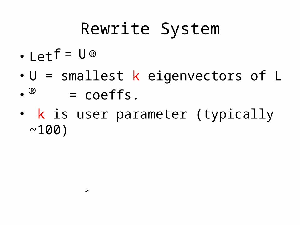
Rewrite System
• Let • U = smallest k eigenvectors of L• = coeffs. • k is user parameter (typically ~100)
• Optimal is now solution to k x k system:
®
(§ + UT ¤U)®= UT ¤y
f = U®
®
Computational Bottleneck
• Consider a dataset of 80 million images
• Inverting L– Inverting 80 million x 80 million matrix
• Finding eigenvectors of L– Diagonalizing 80 million x 80 million
matrix
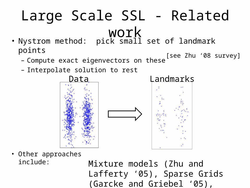
Large Scale SSL - Related work• Nystrom method: pick small set of landmark points
– Compute exact eigenvectors on these– Interpolate solution to rest
• Other approaches include:
[see Zhu ‘08 survey]
Data Landmarks
Mixture models (Zhu and Lafferty ‘05), Sparse Grids (Garcke and Griebel ‘05), Sparse Graphs (Tsang and Kwok ‘06)

Our Approach

Overview of Our Approach• Compute approximate eigenvectors
Data LandmarksDensity
Reduce n
Limit as n ∞
Nystrom
Ours
Linear in number of data-points
Polynomial in number of landmarks
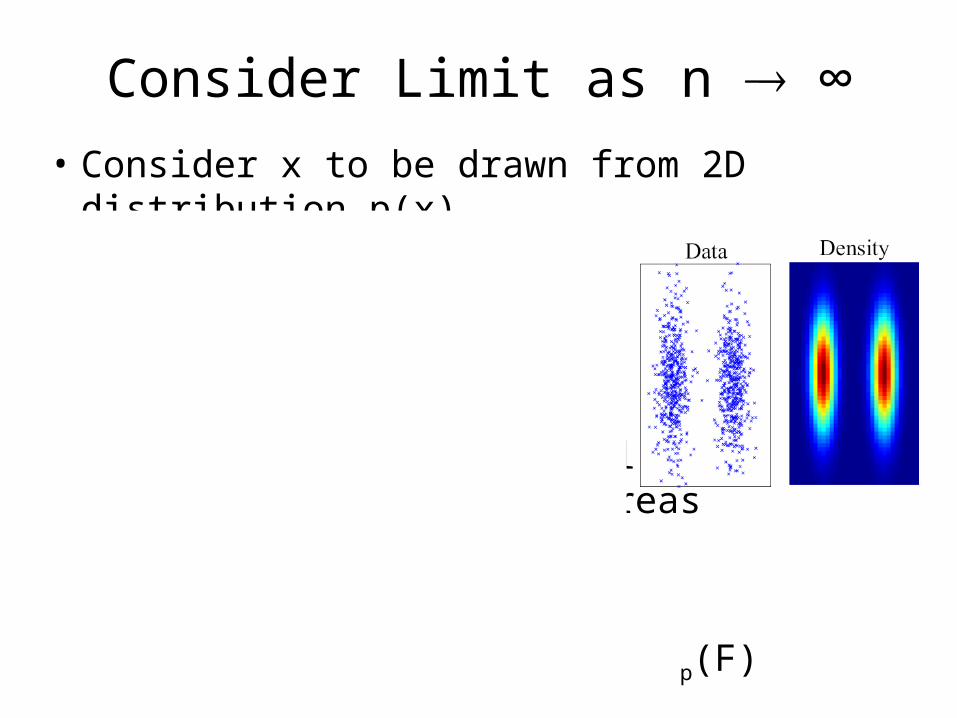
Consider Limit as n ∞
• Consider x to be drawn from 2D distribution p(x)
• Let Lp(F) be a smoothness operator on p(x), for a function F(x)
• Smoothness operator penalizesfunctions that vary in areasof high density
• Analyze eigenfunctions of Lp(F)
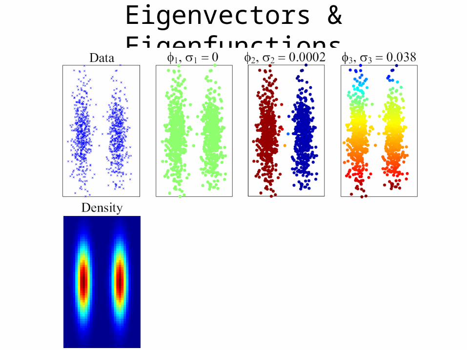
Eigenvectors & Eigenfunctions
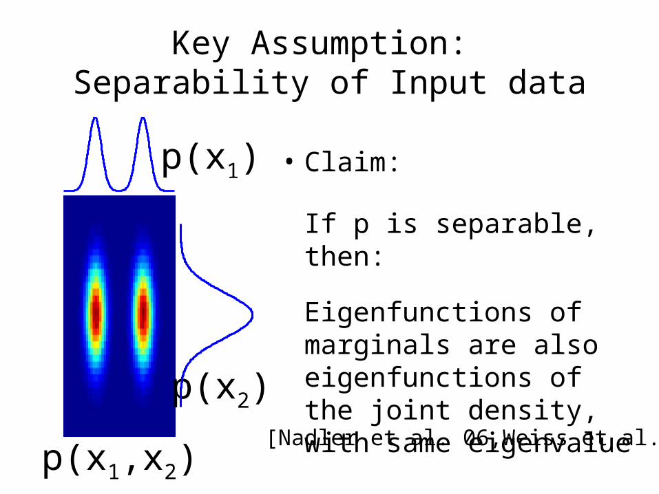
• Claim:
If p is separable, then:
Eigenfunctions of marginals are also eigenfunctions of the joint density, with same eigenvalue
p(x1,x2)
p(x1)
p(x2)
Key Assumption: Separability of Input data
[Nadler et al. 06,Weiss et al. 08]
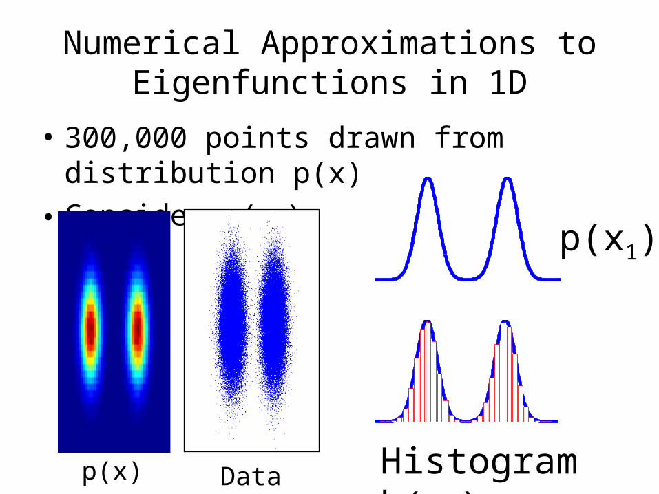
Numerical Approximations to Eigenfunctions in 1D
• 300,000 points drawn from distribution p(x)
• Consider p(x1)
p(x) Data
p(x1)
Histogram h(x1)
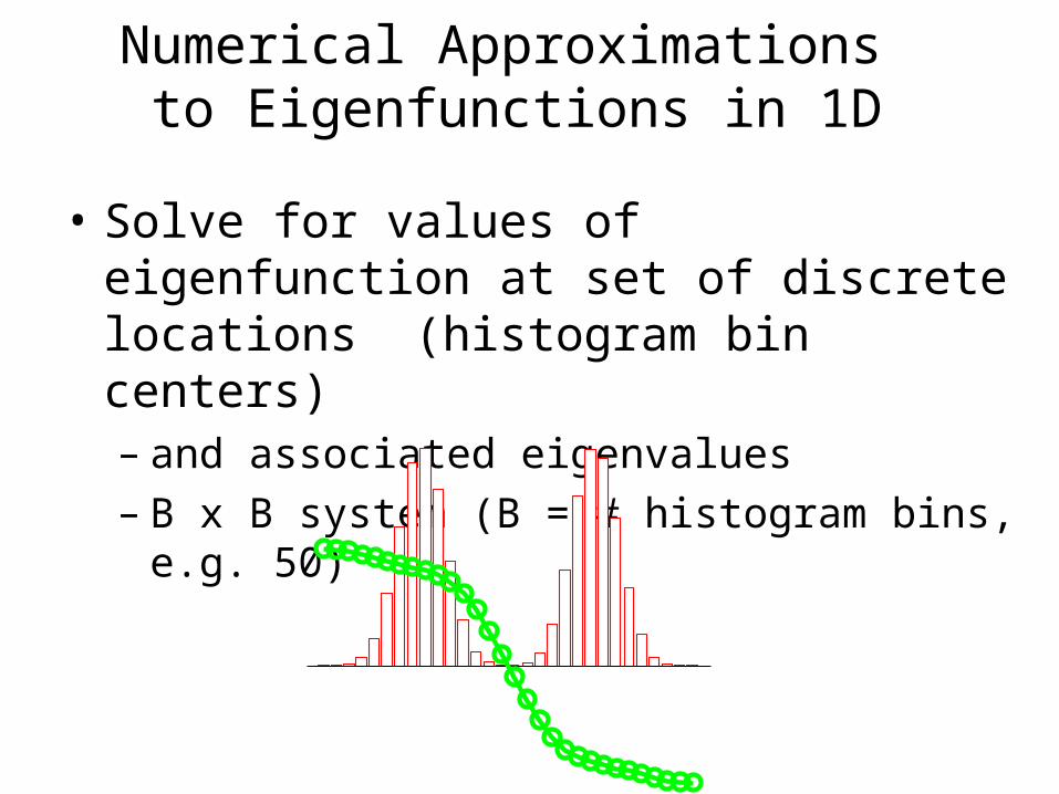
• Solve for values of eigenfunction at set of discrete locations (histogram bin centers)– and associated eigenvalues– B x B system (B = # histogram bins, e.g.
50)
Numerical Approximations to Eigenfunctions in 1D
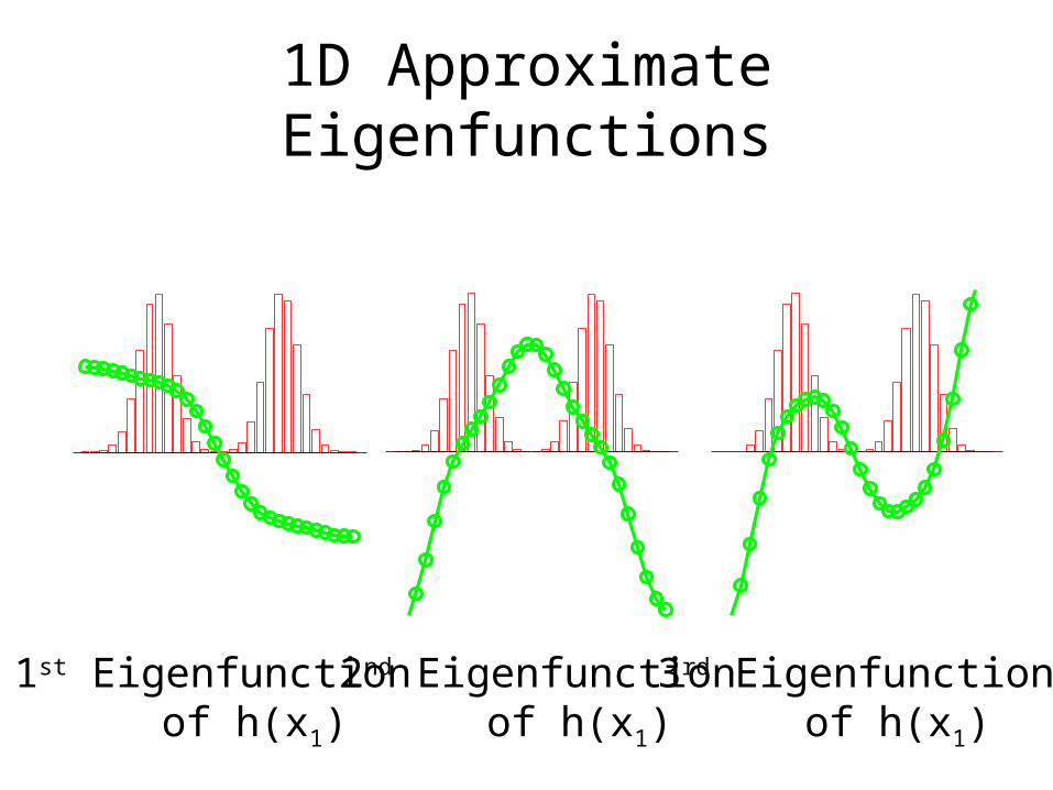
1D Approximate Eigenfunctions
1st Eigenfunction of h(x1)
2nd Eigenfunction of h(x1)
3rd Eigenfunction of h(x1)

Separability over Dimension
• Build histogram over dimension 2: h(x2)
• Now solve for eigenfunctions of h(x2)
1st Eigenfunction of h(x2)
2nd Eigenfunction of h(x2)
3rd Eigenfunction of h(x2)
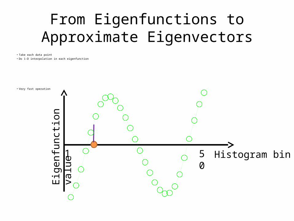
• Take each data point• Do 1-D interpolation in each eigenfunction
• Very fast operation
From Eigenfunctions to Approximate Eigenvectors
Histogram bin1 50
Eig
enfu
nct
ion
valu
e
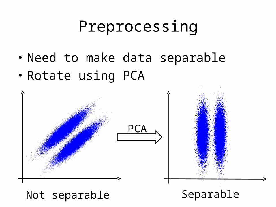
Preprocessing
• Need to make data separable• Rotate using PCA
Not separable Separable
PCA
Overall Algorithm1. Rotate data to maximize separability (currently
use PCA)
2. For each of the d input dimensions:– Construct 1D histogram– Solve numerically for eigenfunctions/values
3. Order eigenfunctions from all dimensions by increasing eigenvalue & take first k
4. Interpolate data into k eigenfunctions– Yields approximate eigenvectors of Laplacian
5. Solve k x k least squares system to give label function

Experimentson Toy Data
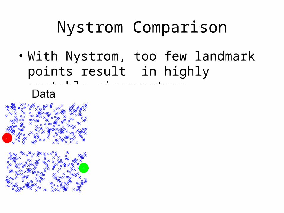
Nystrom Comparison
• With Nystrom, too few landmark points result in highly unstable eigenvectors

Nystrom Comparison
• Eigenfunctions fail when data has significant dependencies between dimensions
Experimentson Real Data
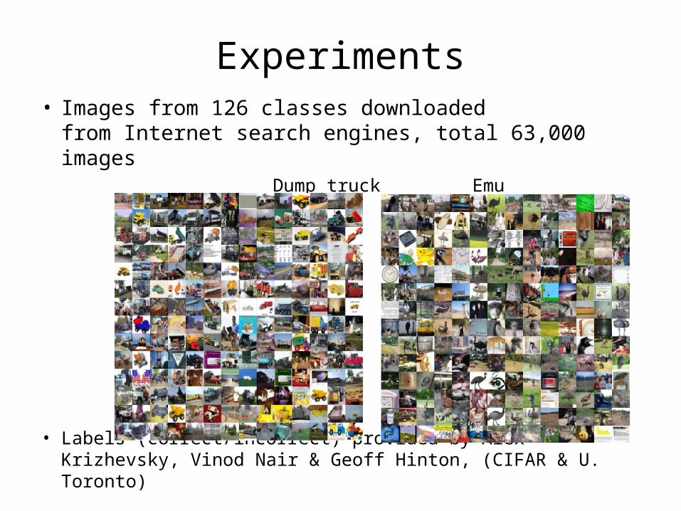
Experiments• Images from 126 classes downloaded
from Internet search engines, total 63,000 images Dump truck Emu
• Labels (correct/incorrect) provided by Alex Krizhevsky, Vinod Nair & Geoff Hinton, (CIFAR & U. Toronto)
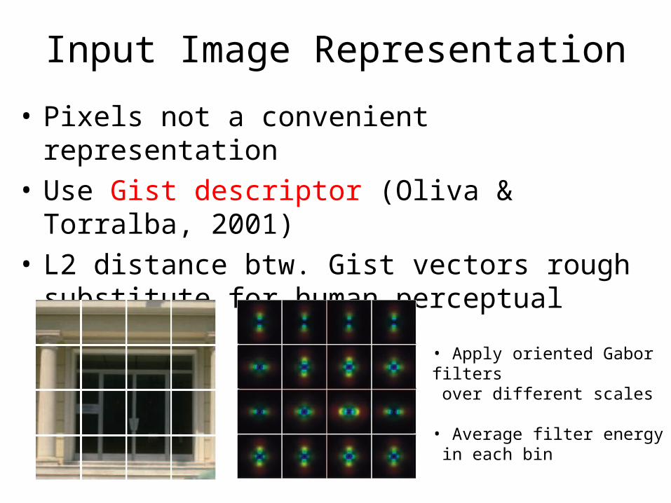
Input Image Representation
• Pixels not a convenient representation• Use Gist descriptor (Oliva & Torralba, 2001)• L2 distance btw. Gist vectors rough
substitute for human perceptual distance
• Apply oriented Gabor filters over different scales
• Average filter energy in each bin
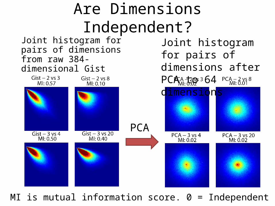
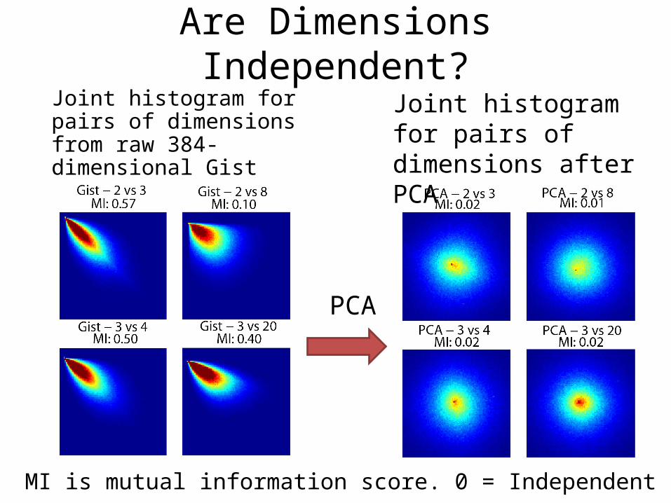
Are Dimensions Independent?Joint histogram for pairs of dimensions from raw 384-dimensional Gist
PCA
Joint histogram for pairs of dimensions after PCA to 64 dimensions
MI is mutual information score. 0 = Independent
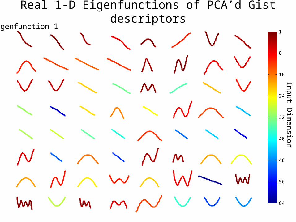
Real 1-D Eigenfunctions of PCA’d Gist descriptors
64
56
48
40
32
24
16
8
1Eigenfunction 1
Inp
ut D
imensio
n
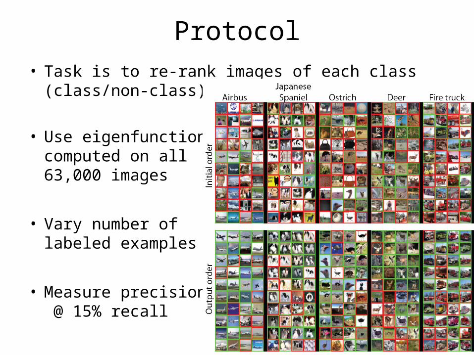
Protocol• Task is to re-rank images of each class
(class/non-class)
• Use eigenfunctionscomputed on all63,000 images
• Vary number of labeled examples
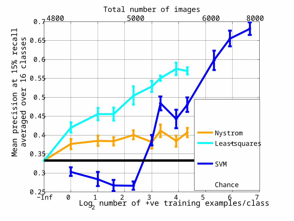
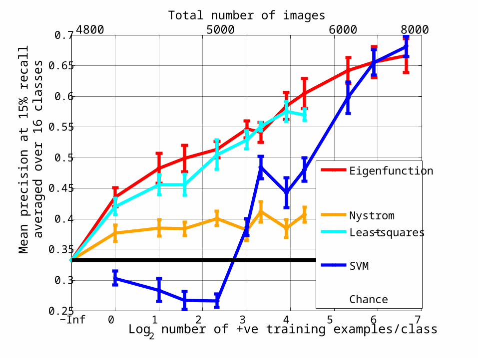
• Measure precision @ 15% recall

−Inf 0 1 2 3 4 5 6 70.25
0.3
0.35
0.4
0.45
0.5
0.55
0.6
0.65
0.7
Log2 number of +ve training examples/class
Mean
pre
cisi
on
at
15
% r
eca
ll a
vera
ged
over
16
cla
sses
Least−squares
SVM
Chance
Total number of images4800 5000 80006000
−Inf 0 1 2 3 4 5 6 70.25
0.3
0.35
0.4
0.45
0.5
0.55
0.6
0.65
0.7
Log2 number of +ve training examples/class
Mean
pre
cisi
on
at
15
% r
eca
ll a
vera
ged
over
16
cla
sses
Nystrom
Least−squares
SVM
Chance
Total number of images4800 5000 80006000
−Inf 0 1 2 3 4 5 6 70.25
0.3
0.35
0.4
0.45
0.5
0.55
0.6
0.65
0.7
Log2 number of +ve training examples/class
Mean
pre
cisi
on
at
15
% r
eca
ll a
vera
ged
over
16
cla
sses
Eigenfunction
Nystrom
Least−squares
SVM
Chance
Total number of images4800 5000 80006000

−Inf 0 1 2 3 4 5 6 70.25
0.3
0.35
0.4
0.45
0.5
0.55
0.6
0.65
0.7
Log2 number of +ve training examples/class
Mean
pre
cisi
on
at
15
% r
eca
ll a
vera
ged
over
16
cla
sses
Eigenfunction
Nystrom
Least−squares
Eigenvector
SVM
NN
Chance
Total number of images4800 5000 80006000

80 Million Images
Running on 80 million images
• PCA to 32 dims, k=48 eigenfunctions
• For each class, labels propagating through 80 million images
• Precompute approximate eigenvectors (~20Gb)
• Label propagation is fast <0.1secs/keyword
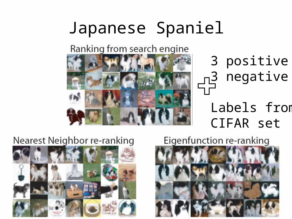
Japanese Spaniel
3 positive3 negative
Labels from CIFAR set
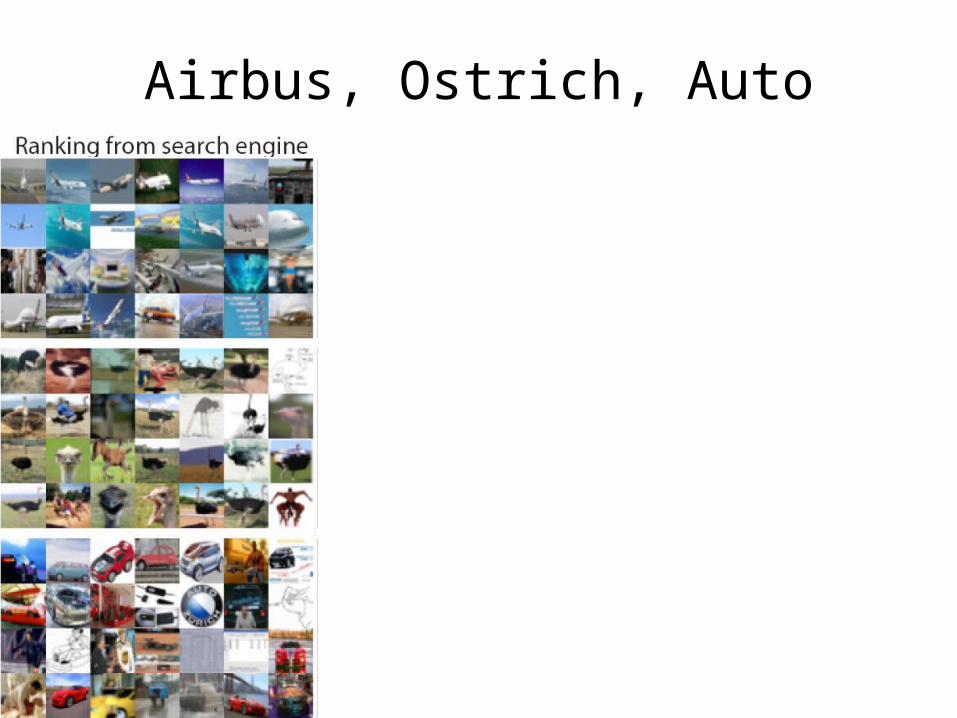
Airbus, Ostrich, Auto
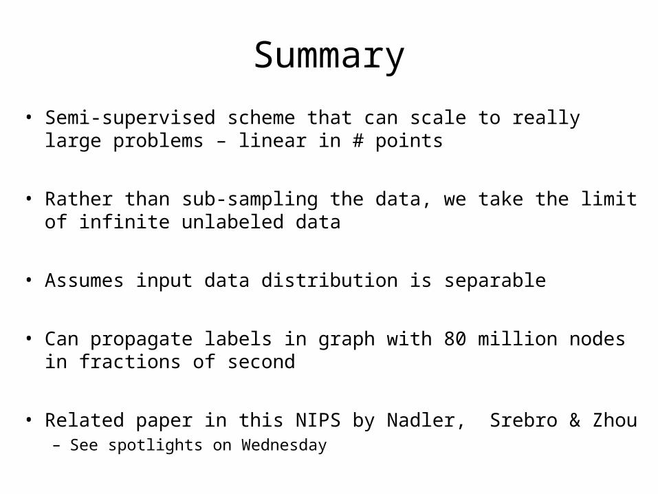
Summary
• Semi-supervised scheme that can scale to really large problems – linear in # points
• Rather than sub-sampling the data, we take the limit of infinite unlabeled data
• Assumes input data distribution is separable
• Can propagate labels in graph with 80 million nodes in fractions of second
• Related paper in this NIPS by Nadler, Srebro & Zhou– See spotlights on Wednesday

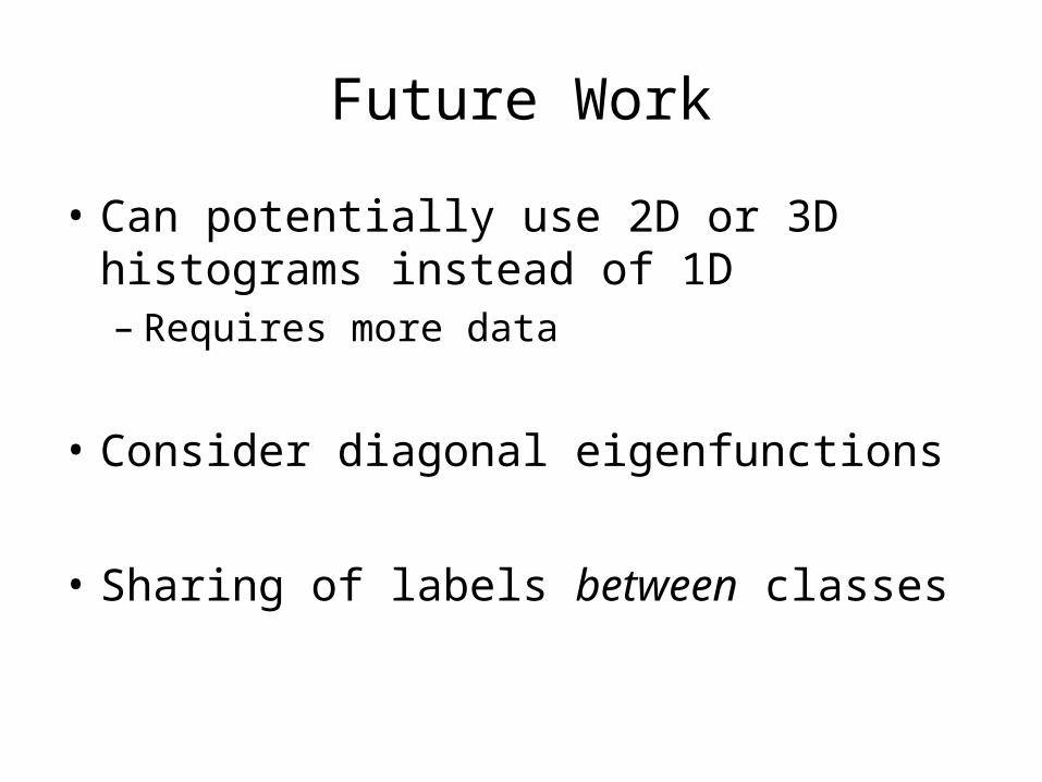
Future Work
• Can potentially use 2D or 3D histograms instead of 1D– Requires more data
• Consider diagonal eigenfunctions
• Sharing of labels between classes
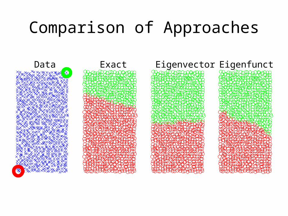
Comparison of Approaches
Data Exact Eigenvector Eigenfunction
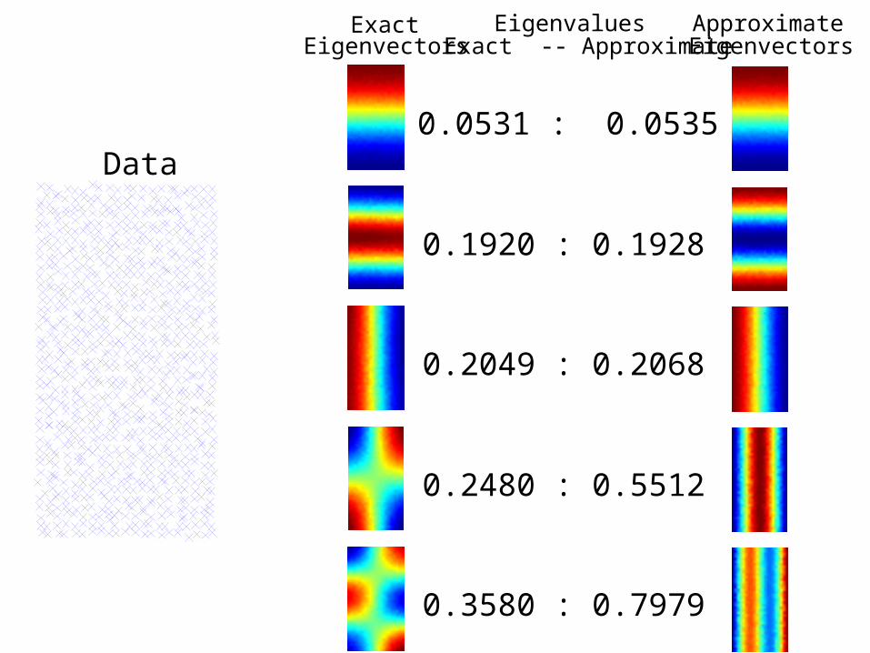
Data
ExactEigenvectors
0.0531 : 0.0535
Exact -- ApproximateEigenvalues Approximate
Eigenvectors
0.1920 : 0.1928
0.2049 : 0.2068
0.2480 : 0.5512
0.3580 : 0.7979
Are Dimensions Independent?Joint histogram for pairs of dimensions from raw 384-dimensional Gist
PCA
Joint histogram for pairs of dimensions after PCA
MI is mutual information score. 0 = Independent
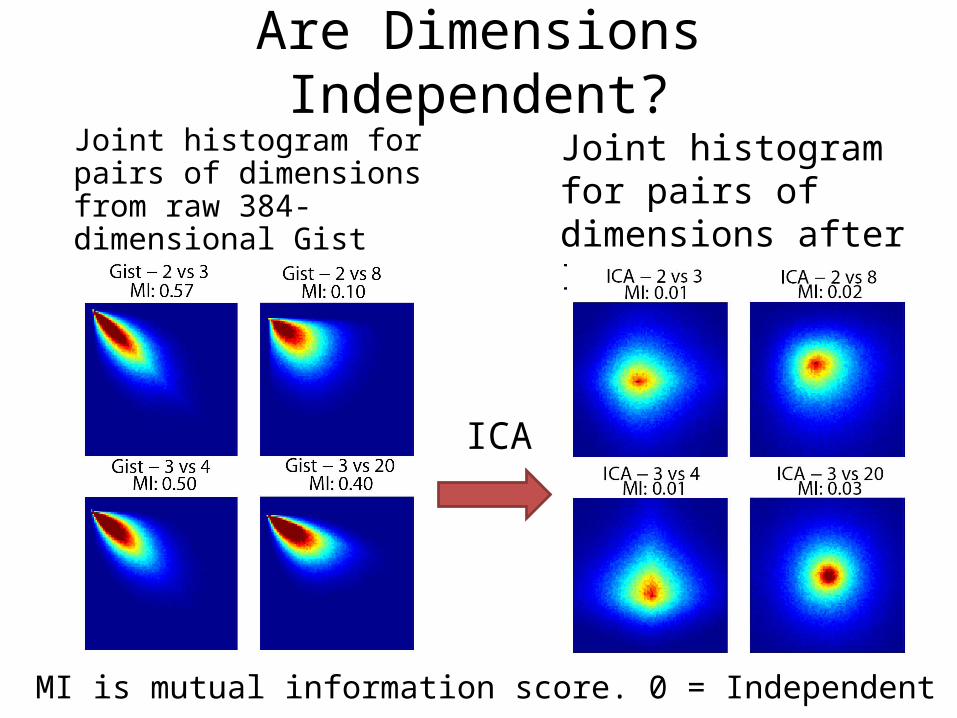
Are Dimensions Independent?Joint histogram for pairs of dimensions from raw 384-dimensional Gist
ICA
Joint histogram for pairs of dimensions after ICA
MI is mutual information score. 0 = Independent
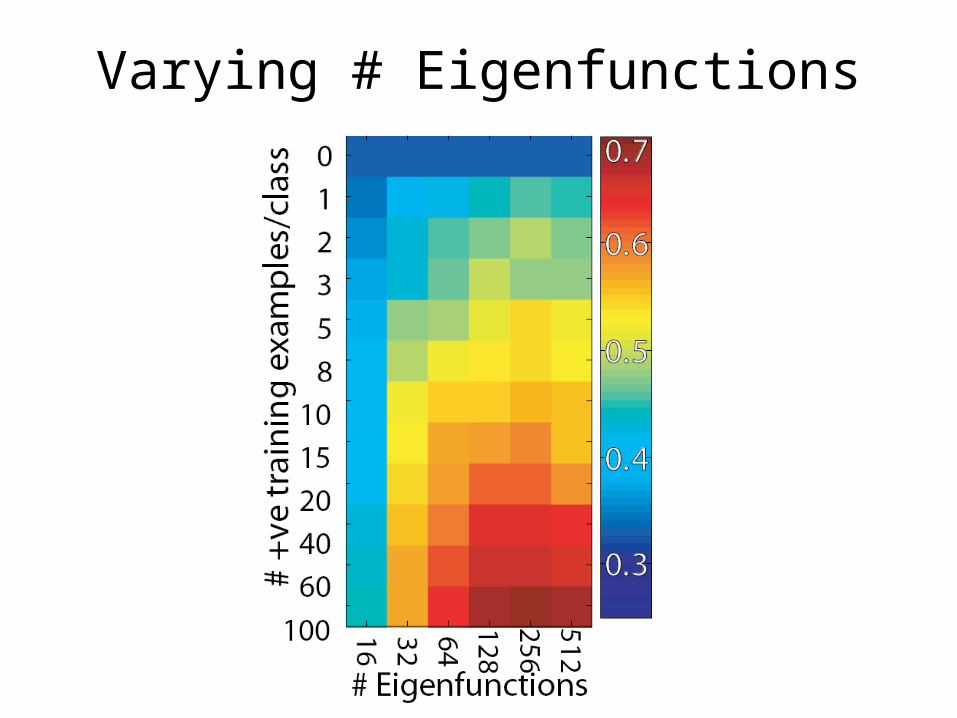
Varying # Eigenfunctions
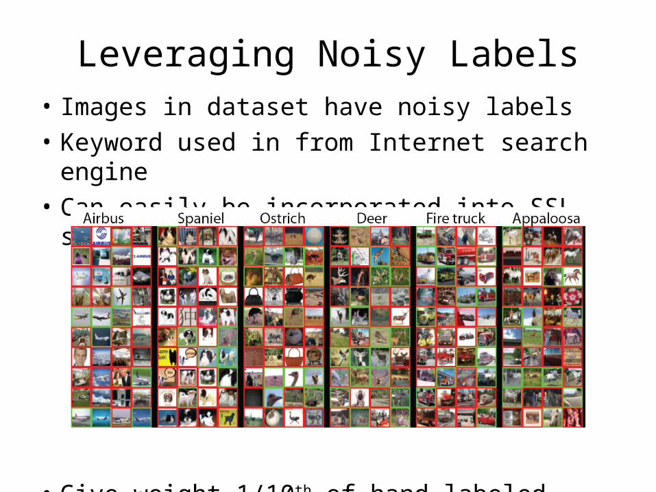
Leveraging Noisy Labels• Images in dataset have noisy labels• Keyword used in from Internet search
engine• Can easily be incorporated into SSL
scheme
• Give weight 1/10th of hand-labeled example
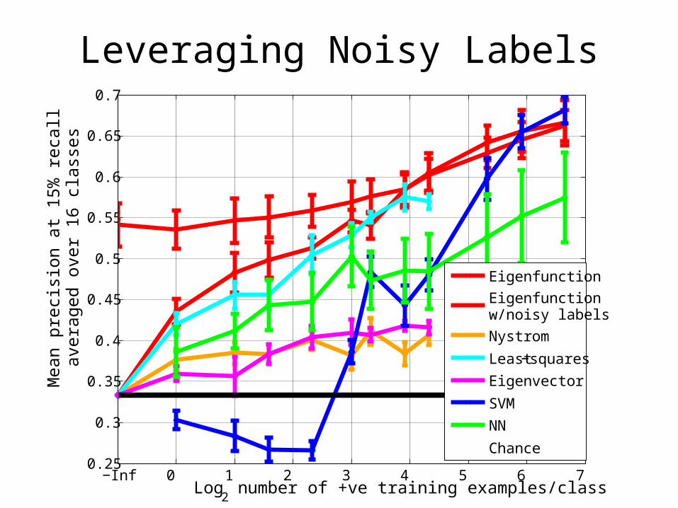
Leveraging Noisy Labels
−Inf 0 1 2 3 4 5 6 70.25
0.3
0.35
0.4
0.45
0.5
0.55
0.6
0.65
0.7
Log2 number of +ve training examples/class
Mean
pre
cisi
on
at
15
% r
eca
ll a
vera
ged
over
16
cla
sses
Eigenfunction
Eigenfunctionw/noisy labels
Nystrom
Least−squares
Eigenvector
SVM
NN
Chance
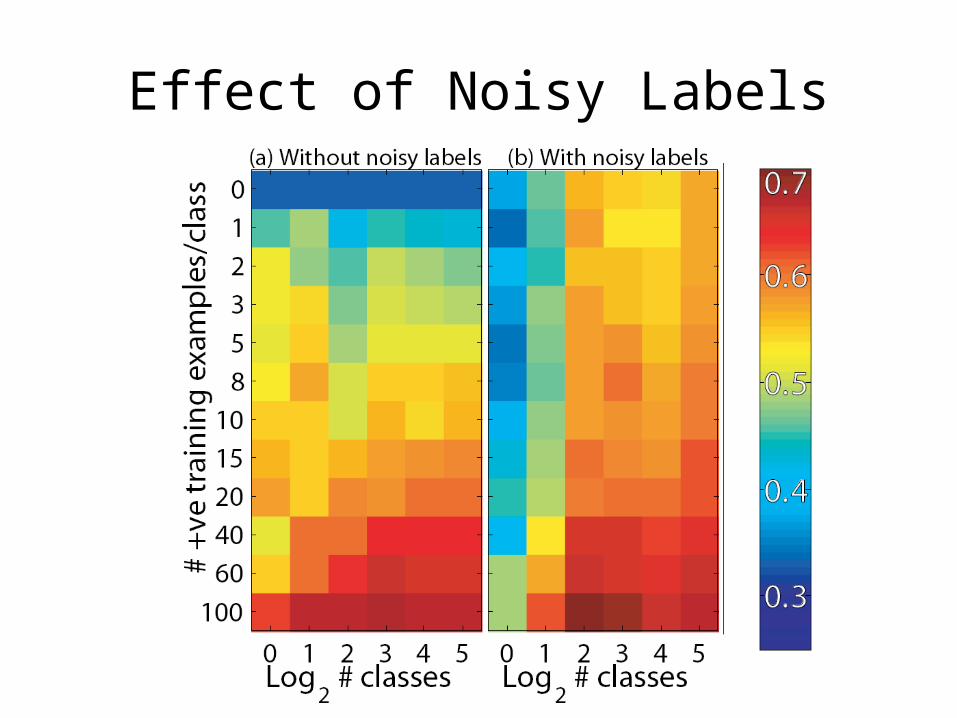
Effect of Noisy Labels
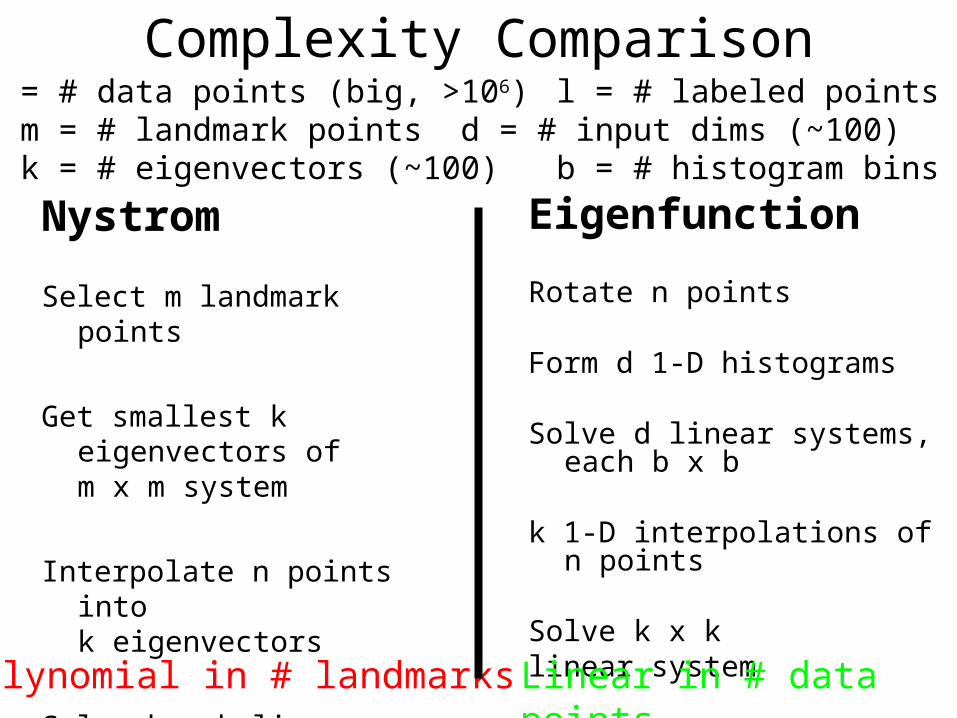
Complexity Comparison
Nystrom
Select m landmark points
Get smallest k eigenvectors of m x m system
Interpolate n points into k eigenvectors
Solve k x k linear system
Eigenfunction
Rotate n points
Form d 1-D histograms
Solve d linear systems, each b x b
k 1-D interpolations of n points
Solve k x k linear system
Key: n = # data points (big, >106) l = # labeled points (small, <100) m = # landmark points d = # input dims (~100) k = # eigenvectors (~100) b = # histogram bins (~50)
Polynomial in # landmarks Linear in # data points
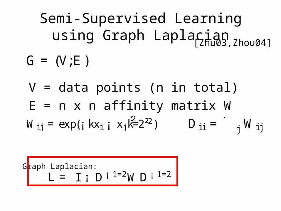
Semi-Supervised Learning using Graph Laplacian
V = data points (n in total)E = n x n affinity matrix W
G = (V;E )
Wi j = exp(¡ kxi ¡ xj k=2²2) Di i =P
j Wi j
L = D ¡ 1=2LD ¡ 1=2 = I ¡ D ¡ 1=2WD ¡ 1=2Graph Laplacian:
[Zhu03,Zhou04]
Wi j = exp(¡ kxi ¡ xj k=2²2)
L = D ¡ 1=2LD ¡ 1=2 = I ¡ D ¡ 1=2WD ¡ 1=2
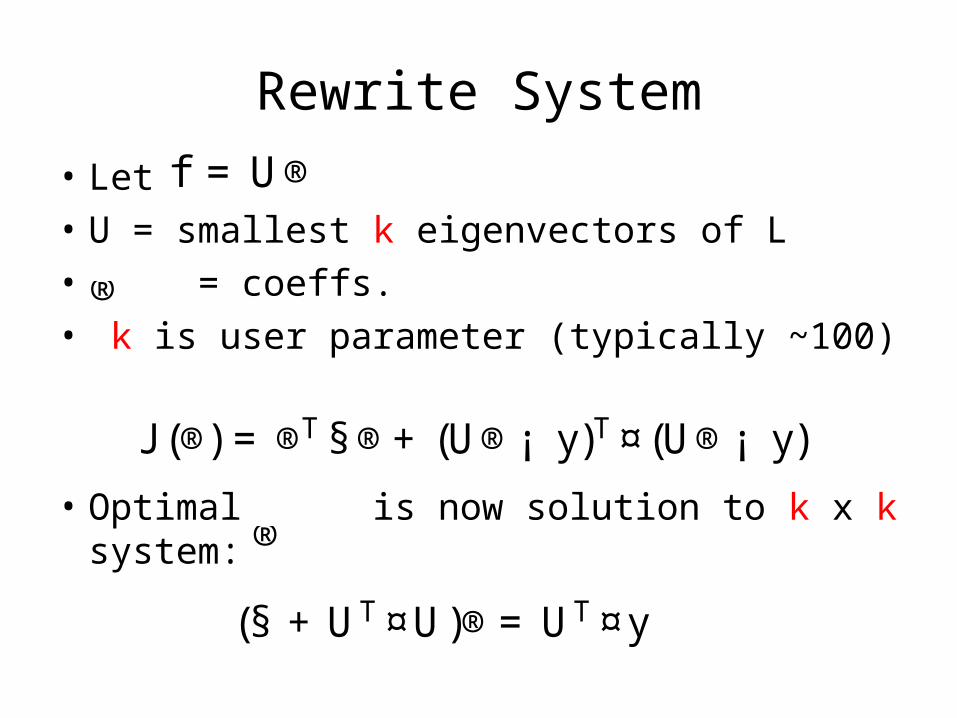
Rewrite System
• Let • U = smallest k eigenvectors of L• = coeffs. • k is user parameter (typically ~100)
• Optimal is now solution to k x k system:
J (®) = ®T § ®+ (U®¡ y)T ¤(U®¡ y)
®
(§ + UT ¤U)®= UT ¤y
f = U®
®
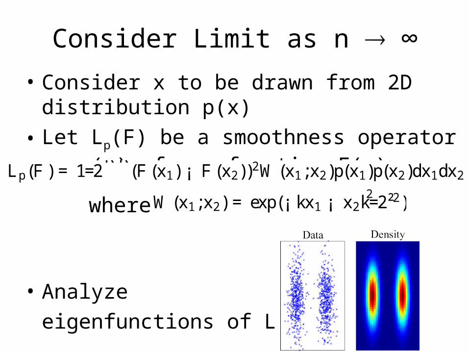
Consider Limit as n ∞
• Consider x to be drawn from 2D distribution p(x)
• Let Lp(F) be a smoothness operator on p(x), for a function F(x):
• Analyze eigenfunctions of Lp(F)
Lp(F ) = 1=2RR
(F (x1) ¡ F (x2))2W(x1;x2)p(x1)p(x2)dx1dx2
W(x1;x2) = exp(¡ kx1 ¡ x2k=2²2)where2
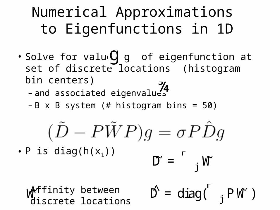
• Solve for values g of eigenfunction at set of discrete locations (histogram bin centers)– and associated eigenvalues– B x B system (# histogram bins = 50)
• P is diag(h(x1))
Numerical Approximations to Eigenfunctions in 1D
~D =P
j~W
~W D̂ = diag(P
j P ~W)
¾
Affinity between discrete locations
P ( ~D ¡ ~W)P g= ¾P D̂g

Real 1-D Eigenfunctions of PCA’d Gist descriptors
64
56
48
40
32
24
16
8
1Eigenfunction 1
Eigenfunction 256
Inp
ut D
imensio
n


