This article was downloaded by: [Indian Institute of Technology - Delhi]On: 22 February 2015, At: 19:33Publisher: Taylor & FrancisInforma Ltd Registered in England and Wales Registered Number: 1072954 Registeredoffice: Mortimer House, 37-41 Mortimer Street, London W1T 3JH, UK

Click for updates

International Journal of RemoteSensingPublication details, including instructions for authors andsubscription information:http://www.tandfonline.com/loi/tres20

Cloud climatology over the oceanicregions adjacent to the IndianSubcontinent: inter-comparisonbetween passive and active sensorsSagnik Deya, Nidhi Nishanta, Kamalika Senguptaa & Sudipta Ghosha

a Centre for Atmospheric Sciences, Indian Institute of TechnologyDelhi, Hauz Khas, New Delhi 110016, IndiaPublished online: 17 Feb 2015.

To cite this article: Sagnik Dey, Nidhi Nishant, Kamalika Sengupta & Sudipta Ghosh (2015) Cloudclimatology over the oceanic regions adjacent to the Indian Subcontinent: inter-comparisonbetween passive and active sensors, International Journal of Remote Sensing, 36:3, 899-916

To link to this article: http://dx.doi.org/10.1080/01431161.2014.1001082

PLEASE SCROLL DOWN FOR ARTICLE

Taylor & Francis makes every effort to ensure the accuracy of all the information (the“Content”) contained in the publications on our platform. However, Taylor & Francis,our agents, and our licensors make no representations or warranties whatsoever as tothe accuracy, completeness, or suitability for any purpose of the Content. Any opinionsand views expressed in this publication are the opinions and views of the authors,and are not the views of or endorsed by Taylor & Francis. The accuracy of the Contentshould not be relied upon and should be independently verified with primary sourcesof information. Taylor and Francis shall not be liable for any losses, actions, claims,proceedings, demands, costs, expenses, damages, and other liabilities whatsoever orhowsoever caused arising directly or indirectly in connection with, in relation to or arisingout of the use of the Content.

This article may be used for research, teaching, and private study purposes. Anysubstantial or systematic reproduction, redistribution, reselling, loan, sub-licensing,systematic supply, or distribution in any form to anyone is expressly forbidden. Terms &

Conditions of access and use can be found at http://www.tandfonline.com/page/terms-and-conditions

Dow

nloa

ded

by [

Indi

an I

nstit

ute

of T

echn

olog

y -

Del

hi]

at 1

9:33

22

Febr

uary

201

5

Cloud climatology over the oceanic regions adjacent to the IndianSubcontinent: inter-comparison between passive and active sensors

Sagnik Dey*, Nidhi Nishant†, Kamalika Sengupta‡, and Sudipta Ghosh

Centre for Atmospheric Sciences, Indian Institute of Technology Delhi, Hauz Khas, New Delhi110016, India

(Received 25 June 2014; accepted 27 November 2014)

Understanding the cloud vertical structure and its variation in space and time is importantto reduce the uncertainty in climate forcing. Here, we present the cloud climatology overthe oceanic regions (Arabian Sea, Bay of Bengal, and South Indian Ocean) adjacent to theIndian subcontinent using data from the Multiangle Imaging Spectroradiometer (MISR),Moderate Resolution Imaging Spectroradiometer (MODIS), GCM-Oriented CALIPSOCloud Product (GOCCP), and International Satellite Cloud Climatology Project (ISCCP).Fractional cloud cover (fc) shows stronger seasonal variations over the Arabian Sea (meanannual fc lies in the range 0.5–0.61) and Bay of Bengal (mean annual fc lies in the range0.69–0.75) relative to the South Indian Ocean (mean annual fc lies in the range 0.64–0.71).Inter-comparison of statistics from passive (MISR, MODIS and ISCCP) and active(GOCCP) sensors reveals the challenges in interpreting satellite data for climate implica-tions. While MISR detects more low clouds because of its stereo technique, MODIS andISCCP detect more high clouds because of their radiometric techniques. Therefore, acombination of these two techniques in passive sensors may lead to more realistic under-standing of the cloud vertical structure. GOCCP (active sensor) can detect multilayercloud, but accuracy reduces if the high clouds are optically thick. A dominance of low andhigh clouds throughout the year is observed in these regions, where cumulus and cirrusdominate among low and high clouds, respectively.

1. Introduction

Aerosol–cloud–radiation interaction continues to be the largest source of uncertainty inquantifying anthropogenic climate change (IPCC 2007; Goren and Rosenfeld 2014;Altaratz et al. 2014). Large discrepancy among climate models in simulating clouds poses achallenge in resolving this critical problem (e.g. Zhang et al. 2005; Probst et al. 2012; Kleinet al. 2013). Evaluation of model-simulated cloud distribution against satellite-based observa-tion (e.g. Randall et al. 2003) at global and regional scales and inter-comparison of statisticsfrom various sensors are required to address this issue (Stubenrauch et al. 2013). In addition tothe cloud fraction, cloud vertical distribution (relative to aerosol vertical distribution) isequally important for improved estimates of radiative forcing.

Ground-based active remote sensing (e.g. lidar or radar) can be utilized to study thevertical distribution of clouds (Xi et al. 2010), but its limited spatial coverage, particularlyover oceanic regions, restricts its applicability for regional scale study. Numerous passive

*Corresponding author. Email: sagnik@cas.iitd.ac.in†Present address: Climate Change Research Center, University of New South Wales, Sydney,Australia.‡Present address: School of Earth and Environment, University of Leeds, LS2 9JT, Leeds, UnitedKingdom.

International Journal of Remote Sensing, 2015Vol. 36, No. 3, 899–916, http://dx.doi.org/10.1080/01431161.2014.1001082

© 2015 Taylor & Francis

Dow

nloa

ded

by [

Indi

an I

nstit

ute

of T

echn

olog

y -

Del

hi]

at 1

9:33

22

Febr

uary

201

5

sensors (e.g. sensors considered for the International Satellite Cloud Climatology Project(ISCCP), the Advanced Very High Resolution Radiometer (AVHRR), and the ModerateResolution Imaging Spectroradiometer (MODIS)) have been using radiometric techniquesfor cloud retrieval, but they cannot retrieve cloud vertical structure at high vertical resolution.Retrieval of cloud vertical structure by passive remote sensing became possible with theadvent of the stereo technique of the Multiangle Imaging Spectroradiometer (MISR) (DiGirolamo et al. 2010), which has been compared against the other passive (e.g. Naudet al. 2004; Marchand et al. 2010) and ground-based active sensors (Marchand, Ackerman,and Moroney 2007). Launches of Cloud-Aerosol Lidar and Pathfinder Satellite Observations(CALIPSO) and CloudSat in 2006 have provided a great opportunity to address this issue atvarious spatial and temporal scales (Anselmo et al. 2007; Verlinden, Thompson, andStephens 2011; Nair et al. 2011; Meenu et al. 2010, 2011); however, the sampling noisedue to the narrow swaths of the active space-borne sensors may be a concern in such inter-comparison. More observations over the years will resolve the sampling issue for the activesensors. Since cloud detection is a challenging task due to the influences of many remote-sensing artefacts such as misclassification of clear and cloudy pixels, shadow effect, and sunglint, as summarized in Loeb and Schuster (2008), there is a need to inter-compare multi-sensor data sets utilizing different retrieval techniques to understand the strengths andweaknesses of individual sensors. The importance of the issue led to an international effortinitiated in 2005 under the umbrella of Global Energy and Water Cycle Experiment, whichpublished its first coordinated inter-comparison of global cloud properties (Stubenrauchet al. 2013). More regional analysis (Jin, Hanesiak, and Barber 2007; Kühnlein et al. 2013),particularly in the regions affected by seasonal cycle of synoptic meteorology (e.g. Indiansubcontinent), is warranted to fully understand the utility of satellite-based cloud products. Inthe present work, we utilize ten years of passive and five years of active remote-sensing data toexamine the vertical distribution of clouds and its space-time variability over the oceanicregions adjacent to the Indian subcontinent.

The study area became a test bed for examining aerosol–cloud interaction, forwhich cloud vertical distribution is an important parameter (Chand et al. 2009), eversince the Indian Ocean Experiment (Ramanathan, Crutzen, Kiehl, et al. 2001). TheArabian Sea, Bay of Bengal and South Indian Ocean experience a reversal in winddirection from southwesterly during June to September to northeasterly during thewinter months. The contrasting synoptic meteorology controls the precipitation patternin the subcontinent and modulates aerosol characteristics by transporting polluted airfrom the land to the ocean during the winter season (Ramanathan, Crutzen, Kiehl,et al. 2001). Also, cloud detection is easier over ocean relative to land due tohomogeneous surface reflectance (excluding the glint-affected areas), and hence, theinter-comparison will help better understanding of the strength and weakness of theretrieval techniques in detecting cloud vertical structure.

Variability of clouds over global oceans has been examined from 55 years ofsurface observations (Eastman, Warren, and Hahn 2011). However, very few studiesexist in the Indian Continental Tropical Convergence Zone. Combined analysis ofISCCP and Earth Radiation Budget Experiment flux data for the period 1985–1988was carried out by Rajeevan and Srinivasan (1999) to understand the variability ofcloud radiative forcing (CRF) in this region. Using the same data sets, Patil andYadav (2005) have estimated much larger shortwave (SW) cooling than longwave(LW) warming for the monsoon clouds over the Indian region. The resulting netcooling at the top-of-the-atmosphere (TOA) was found to be larger over the Bay ofBengal relative to the Arabian Sea in the monsoon season due to a larger fractional

900 S. Dey et al.

Dow

nloa

ded

by [

Indi

an I

nstit

ute

of T

echn

olog

y -

Del

hi]

at 1

9:33

22

Febr

uary

201

5

cloud cover (fc) facilitated by the upper tropospheric easterly jet (Sathiyamoorthy, Pal,and Joshi 2011). From a satellite point of view, fc is defined as the fraction of cloudypixels in the total number of pixels within a given domain. Wonsick, Pinker, andGovaerts (2009) examined the diurnal variation of fc over the Indian region usingMeteosat observations and observed that the daytime diurnal cycles are flat, U-shaped,and ascending towards an afternoon peak during the pre-monsoon, monsoon, and post-monsoon seasons, respectively. Meenu et al. (2010, 2011) examined the variability ofhigh clouds over the subcontinent using CALIPSO data and reported occurrence of thedeepest clouds (12 K lower than other deep convective regions) over the northern Bayof Bengal during June–August. Nair et al. (2011) found a ‘pool of inhibited cloudi-ness’ over the Bay of Bengal during the monsoon months by combining CloudSat andAVHRR data. Most of these studies used satellite data of limited period of time. Forexample, Bony, Collins, and Fillmore (2000) examined the variability of low clouds inthe winter season during 1986–1989 and observed that the Arabian Sea and Bay ofBengal are dominated by cumulus clouds, while the South Indian Ocean is dominatedby stratocumulus clouds. Moreover, they are confined to mostly passive remotesensing. Therefore, there is a need to understand the space–time variability of cloudsfor a longer period of time, and more particularly, their vertical distributions in theIndian monsoon region in the recent years. Changes in precipitation pattern over theIndian monsoon region in the recent years (Goswami et al. 2006; Dash et al. 2009)further emphasize the importance to understand the variability of cloud verticalstructure.

Here, we present a monthly climatology of fc over the Arabian sea, Bay ofBengal, and South Indian Ocean derived from MISR and MODIS for the periodMarch 2000–February 2010, GCM-Oriented CALIPSO Cloud Product (GOCCP) forthe period June 2006–December 2010, and ISCCP for the period January 2000–December 2007. Further, ISCCP data for the period 2000–2007 have been used toexamine the relative abundance of individual cloud types. This will help in inter-preting the observed variability in cloud distribution statistics from passive andactive sensors. The applicability of such climatological statistics for climate studiesis discussed in view of the strengths and weaknesses of the retrieval techniques.

2. Analysis

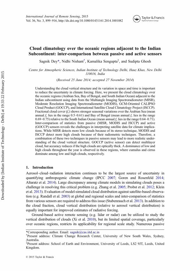
Since our objective is to understand the variability of cloud vertical distribution overthe oceans surrounding the Indian subcontinent, we chose the domain as follows: theArabian Sea bounded by 20° N to the equator and 58–73° E longitude, the Bay ofBengal bounded by 20° N to the equator and 86–94° E, and the South Indian Oceanbounded by the equator to 20° S and 58–94° E longitude (Figure 1). We analysedMISR cloud fraction by altitude (CFbA) and MODIS cloud products for ten years(March 2000–February 2010), GOCCP-fc for five years (June 2006–December 2010)and ISCCP data for eight years (January 2000–December 2007). Mean monthlystatistics have been generated for fc, its vertical distribution, and relative abundanceof various individual cloud types. fc may vary simply because of different clouddetection techniques (Stubenrauch et al. 2013) and/or different pixel resolutions ofvarious sensors (Zhao and Di Girolamo 2006). While comparing climatology of fcand cloud vertical distribution, only daytime retrievals are considered because MISRcan detect clouds only in daytime. Brief descriptions of the satellite and other dataare provided below.

International Journal of Remote Sensing 901

Dow

nloa

ded

by [

Indi

an I

nstit

ute

of T

echn

olog

y -

Del

hi]

at 1

9:33

22

Febr

uary

201

5

2.1. MISR Data

MISR, on board EOS-Terra, crosses the equator at ~10:30/22:30 local time. It has ninecameras at 0°, ±26.1°, ±45.6°, ±60°, and ±70.5°. Choosing a multi-angle view over asingle nadir viewing sensor ensures almost an order of magnitude improvement in theaccuracy of individual scene albedo and better probing into the cloud vertical height.Cloud top height is determined using the three near nadir cameras 0° and ±26° usingthe stereo technique at 1.1 km × 1.1 km resolution at sufficient spatial contrastbetween cloud and underlying surface (Marchand et al. 2010). This technique doesnot rely on atmospheric thermal structure and is less sensitive to radiometric calibra-tion error (Di Girolamo et al. 2010). The relative frequency of cloud tops at each0.5 km vertical resolution is processed as level 3 daily (and subsequently as monthlyby averaging all daily values) CFbA products gridded globally at 0.5° × 0.5° spatialresolution between the surface and 20 km altitude (Di Girolamo et al. 2010). Detaileddiscussion about the quality of MISR cloud top height retrieval is available in theliterature (e.g. Marchand, Ackerman, and Moroney 2007, 2010; Naud et al. 2004). Inbrief, the major source of error in cloud top height detection stems from ‘windcorrection’ with each 1 m s‒1 error in the along-track wind leading to an error of~100 m in the cloud top height (Marchand et al. 2010). It must be mentioned here thatthis technique relies on the optical depth threshold and thus fails to identify thin(cloud optical depth (COD) in the range 0.1–0.3) and sub-visual cirrus (COD < 0.1)(Prasad and Davies 2012). However, this also allows detection of low-level cloudsbeneath thin cirrus. To compare with columnar fc from MODIS and ISCCP, MISR fcvalues of each altitude bin are summed to derive the columnar fc.

Figure 1. Locations of the study area: the Arabian Sea, Bay of Bengal, and South Indian Ocean.

902 S. Dey et al.

Dow

nloa

ded

by [

Indi

an I

nstit

ute

of T

echn

olog

y -

Del

hi]

at 1

9:33

22

Febr

uary

201

5

2.2. MODIS Data

MODIS is flying on board EOS-Terra along with MISR and also on Aqua (which crossesthe equator at ~13:30/1:30 local time). It uses both SW and thermal infrared bands only atthe nadir view to detect clouds. Multispectral retrieval mitigates the concern of inap-propriate cloud classification while encountering snow and ice conditions. Additionally aCO2 slicing technique (Wylie, Menzel, and Strabala 1994) is employed to distinguishtransmissive clouds from opaque clouds and thus helps to report thin cirrus clouds, whichare often missed by the other sensors (e.g. Ackerman et al. 2002). Cloud masking is doneat 1 km × 1 km resolution and fc is calculated as the ratio of cloudy pixels to the totalnumber of pixels within a domain of 10 km × 10 km (Level 2 data) (Platnick et al. 2003).The level 2 fc is further averaged over 1° × 1° spatial resolution to produce a daily andmonthly level 3 fc product. In the present study, daytime Terra-MODIS derived fc data areanalysed for comparison with MISR-derived fc.

2.3. ISCCP Data

Cloud-type information has been derived from the ISCCP D2 data set (Rossow andSchiffer 1999). ISCCP uses up to five geostationary and two polar orbiting satellites tocalculate fc at three hour intervals. The clouds detected are further classified into ninetypes according to cloud top pressure (CTP) and COD. Clouds are first categorized as‘low clouds’ (when CTP is below 680 hPa altitude), ‘mid-level clouds’ (when CTP liesbetween 440 hPa and 680 hPa altitude), and ‘high clouds’ (when CTP exceeds 440 hPaaltitude). Each of these three cloud types are further subdivided into three categories basedon COD. Low clouds with COD < 3.6, 3.6 < COD < 23, and COD > 23 are classified ascumulus, stratocumulus, and stratus, respectively. The corresponding classes for mid-levelclouds are altocumulus, altostratus, and nimbostratus; while the classes are cirrus, cirros-tratus, and deep convective, respectively, for high clouds. The D2 data set is an improve-ment over the previous data sets because of the reduction of the bias in retrieved cloud toptemperature and pressure. This has been achieved by including effects of infrared scatter-ing, improved low-level cloud sensitivities during the sunrise and sunset, and by changingthe visible radiance threshold test to a visible reflectance threshold test (Rossow andSchiffer 1999). However, very thin clouds (COD < 0.1 over ocean) may be missed byISCCP. In the present study, we analysed ISCCP data at 6 UTC (11:30 am local time),which is in between Terra (10:30 am local time) and CALIPSO (~1:30 pm local time)overpass times to facilitate inter-comparison.

2.4. GOCCP data

Cloud vertical distributions are also available from the GOCCP data sets. The detailedalgorithm is discussed by Chepfer et al. (2010). First, clouds are detected based on thescattering ratio (SR) thresholds in the measured vertical profiles at 333 m resolution below8 km and at 1 km resolution above 8 km. For example, cloudy (SR > 5), clear(0.01 < SR < 1.2), fully attenuated (SR < 0.01), and unclassified (1.2 < SR < 5) layersare identified in the profiles. Then it is determined whether the profile contains at least one‘low cloud’ (CTP below 680 hPa altitude), ‘mid-level cloud’ (440 < CTP <680 hPa), and‘high cloud’ (CTP above 440 hPa altitude). Monthly fc is computed at 40 vertical levelsbetween surface to 19.2 km at 480 m interval, for each 1° × 1° grid box by considering thenumber of cloudy profiles in total SR profiles in one month. Note that this definition is

International Journal of Remote Sensing 903

Dow

nloa

ded

by [

Indi

an I

nstit

ute

of T

echn

olog

y -

Del

hi]

at 1

9:33

22

Febr

uary

201

5

different from the definition of fc (i.e. fraction of cloudy pixels to total number of pixelswithin a scene) in the passive remote sensing. The fully attenuated profiles are notconsidered in generating cloud vertical distributions in GOCCP data sets. This is doneto increase the signal-to-noise ratio and minimize false cloud detection (Chepferet al. 2010). This data set was produced with the view of making satellite observationsof the cloud field more coherent with the ensemble GCM and lidar simulator-simulatedcloud fields (with respect to horizontal and vertical resolution, cloud detection, and clouddiagnostics) so that a comparison between the two could bring out the shortcomings of themodel performance rather than the differences in the methods applied by the model andsimulator outputs and the observations. Thus like most GCMs, this data set has the cloudvertical distribution at 40 altitude bins making it suitable for comparison with MISR.Since CALIOP is an active remote sensor, both day and night-time cloud verticaldistributions are available. For the comparison with other data sets, only daytimeGOCCP data version 2.69 is analysed.

3. Results

3.1. Variability of fcThe temporal variability of fc from various sensors is shown in Figure 2, while the mean (±1standard deviation, σ) monthly statistics are summarized in Table 1. The climatology wasderived from the multi-sensor observations within a 3-hour window (10:30 am–1:30 pm) tominimize the influence of diurnal variability on fc. The seasonal variability of fc is strongover the Arabian Sea and Bay of Bengal, with highest values of fc (0.7–0.9) in the monsoon

1.00.80.60.40.20.0

f c

1.00.80.60.40.20.0

f c

1.0

South Indian Ocean

Bay of Bengal

Arabian Sea

MODIS

MISR

ISCCP

GOCCP

0.80.60.40.20.0

Jun

-00

Jun

-01

Jun

-02

Jun

-03

Jun

-04

Jun

-05

Jun

-06

Jun

-07

Jun

-08

Jun

-09

Dec

-00

Dec

-01

Dec

-02

Dec

-03

Dec

-04

Dec

-05

Dec

-06

Dec

-07

Dec

-08

Dec

-09

f c

Figure 2. Temporal variability of fc from MISR and MODIS (during March 2000–February 2010),ISCCP (during January 2000–December 2007), and GOCCP (during June 2006–February 2010)over the Arabian Sea, Bay of Bengal, and South Indian Ocean.

904 S. Dey et al.

Dow

nloa

ded

by [

Indi

an I

nstit

ute

of T

echn

olog

y -

Del

hi]

at 1

9:33

22

Febr

uary

201

5

Table1.

Mean(±1σ)mon

thly

statisticsof

f cfrom

variou

ssensorsov

ertheArabian

Sea

(1strow),Bay

ofBengal(2nd

row),andSou

thIndian

Ocean

(3rd

row).

MODIS-fc(day)

MISR-fc(day)

ISCCP-fc(day)

GOCCP-fc(day)

GOCCP-fc(night)

MODIS-fc(night)

Tim

eperiod

March

2000–F

ebruary

2010

March

2000–F

ebruary

2010

Janu

ary20

00–D

ecem

ber

2007

June

2006–F

ebruary

2010

June

2006–F

ebruary

2010

March

2000–F

ebruary

2010

January

0.53

±0.05

0.53

±0.04

0.44

±0.05

0.43

±0.07

0.46

±0.04

0.51

±0.05

0.64

±0.04

0.57

±0.05

0.61

±0.06

0.53

±0.03

0.48

±0.05

0.55

±0.02

0.71

±0.06

0.68

±0.06

0.66

±0.04

0.59

±0.02

0.62

±0.04

0.73

±0.02

February

0.40

±0.06

0.43

±0.06

0.44

±0.07

0.38

±0.08

0.35

±0.11

0.39

±0.10

0.52

±0.08

0.45

±0.05

0.49

±0.10

0.51

±0.13

0.45

±0.11

0.50

±0.12

0.70

±0.07

0.67

±0.06

0.65

±0.06

0.65

±0.06

0.69

±0.08

0.78

±0.05

March

0.36

±0.06

0.38

±0.03

0.29

±0.05

0.31

±0.06

0.28

±0.04

0.32

±0.07

0.56

±0.07

0.51

±0.05

0.54

±0.05

0.45

±0.10

0.46

±0.12

0.54

±0.10

0.65

±0.04

0.65

±0.03

0.64

±0.06

0.61

±0.06

0.63

±0.06

0.73

±0.03

April

0.45

±0.06

0.44

±0.03

0.23

±0.09

0.35

±0.06

0.33

±0.05

0.39

±0.05

0.66

±0.06

0.61

±0.07

0.62

±0.06

0.57

±0.07

0.56

±0.06

0.68

±0.05

0.66

±0.06

0.67

±0.03

0.65

±0.06

0.57

±0.04

0.59

±0.04

0.70

±0.04

May

0.66

±0.04

0.65

±0.05

0.55

±0.05

0.58

±0.07

0.57

±0.08

0.66

±0.06

0.84

±0.04

0.81

±0.05

0.75

±0.05

0.77

±0.03

0/76

±0.04

0.86

±0.04

0.61

±0.06

0.67

±0.04

0.64

±0.04

0.57

±0.07

0/59

±0.03

0.65

±0.06

June

0.86

±0.05

0.85

±0.04

0.74

±0.08

0.80

±0.08

0.81

±0.08

0.84

±0.08

0.90

±0.03

0.88

±0.03

0.81

±0.04

0.84

±0.05

0.88

±0.02

0.94

±0.02

0.69

±0.04

0.74

±0.03

0.63

±0.06

0.67

±0.03

0.69

±0.06

0.74

±0.03

July

0.89

±0.03

0.87

±0.03

0.73

±0.05

0.83

±0.03

0.81

±0.05

0.87

±0.03

0.90

±0.03

0.89

±0.02

0.81

±0.03

0.86

±0.04

0.91

±0.03

0.96

±0.02

0.73

±0.03

0.78

±0.03

0.64

±0.04

0.67

±0.04

0.71

±0.03

0.76

±0.03

Augu

st0.79

±0.03

0.80

±0.02

0.64

±0.03

0.79

±0.04

0.77

±0.03

0.80

±0.03

0.90

±0.03

0.88

±0.07

0.81

±0.07

0.85

±0.02

0.90

±0.06

0.95

±0.03

0.71

±0.02

0.77

±0.02

0.64

±0.04

0.69

±0.05

0.73

±0.03

0.77

±0.03

September

0.70

±0.08

0.71

±0.08

0.61

±0.09

0.67

±0.10

0.67

±0.10

0.71

±0.09

0.88

±0.03

0.83

±0.04

0.80

±0.03

0.84

±0.05

0.89

±0.03

0.93

±0.04

0.70

±0.02

0.77

±0.03

0.65

±0.06

0.67

±0.02

0.72

±0.04

0.77

±0.02

(Con

tinued)

International Journal of Remote Sensing 905

Dow

nloa

ded

by [

Indi

an I

nstit

ute

of T

echn

olog

y -

Del

hi]

at 1

9:33

22

Febr

uary

201

5

Table

1.(Con

tinued).

MODIS-fc(day)

MISR-fc(day)

ISCCP-fc(day)

GOCCP-fc(day)

GOCCP-fc(night)

MODIS-fc(night)

Tim

eperiod

March

2000–F

ebruary

2010

March

2000–F

ebruary

2010

Janu

ary20

00–D

ecem

ber

2007

June

2006–F

ebruary

2010

June

2006–F

ebruary

2010

March

2000–F

ebruary

2010

Octob

er0.56

±0.06

0.58

±0.05

0.50

±0.07

0.49

±0.06

0.48

±0.08

0.55

±0.06

0.82

±0.07

0.73

±0.08

0.76

±0.07

0.74

±0.10

0.75

±0.09

0.84

±0.07

0.70

±0.04

0.74

±0.02

0.62

±0.04

0.66

±0.05

0.72

±0.05

0.76

±0.05

Nov

ember

0.54

±0.09

0.54

±0.07

0.54

±0.10

0.47

±0.10

0.43

±0.10

0.55

±0.06

0.73

±0.07

0.67

±0.07

0.73

±0.05

0.63

±0.10

0.64

±0.09

0.75

±0.03

0.70

±0.04

0.73

±0.03

0.65

±0.05

0.65

±0.02

0.70

±0.02

0.76

±0.02

Decem

ber

0.56

±0.09

0.53

±0.07

0.49

±0.09

0.48

±0.04

0.50

±0.07

0.59

±0.03

0.70

±0.06

0.65

±0.06

0.67

±0.05

0.65

±0.09

0.69

±0.06

0.71

±0.06

0.69

±0.08

0.69

±0.07

0.65

±0.04

0.67

±0.09

0.71

±0.07

0.78

±0.07

906 S. Dey et al.

Dow

nloa

ded

by [

Indi

an I

nstit

ute

of T

echn

olog

y -

Del

hi]

at 1

9:33

22

Febr

uary

201

5

(June–September) season as expected, and lowest values (0.4–0.5) in the winter season(December–February) as revealed by the passive (MODIS, MISR, and ISCCP) and active(GOCCP) sensors (Figure 2). GOCCP shows a slight low bias in fc in the monsoon season,which may stem from the way fc is defined as a direct consequence of the lidar limitation.The monsoon season is characterized by the development of optically thick convectiveclouds. If the lidar signal becomes attenuated due to penetration through optically thickclouds, the number of times low-level clouds are detected within a grid will be reduced andthus fc will also be reduced. The passive sensors detect the cloud tops and calculate fc bycounting the number of cloudy pixels within the grid. Seasonal variability of fc is muchlower over the South Indian Ocean compared to the Arabian Sea and Bay of Bengal asshown by the passive and active sensors (Table 1). This may be attributed to less seasonalvariability of synoptic scale meteorology and low aerosol concentration, thereby lessinfluence on cloud formation, over the South Indian Ocean. The mean (±1σ) annual fcvalues over the Arabian Sea are 0.61 ± 0.18, 0.61 ± 0.17, 0.5 ± 0.17, and 0.55 ± 0.19 asestimated by MODIS, MISR, ISCCP, and GOCCP, respectively. The corresponding valuesfor the Bay of Bengal are 0.75 ± 0.14, 0.71 ± 0.16, 0.70 ± 0.12, and 0.69 ± 0.16, and for theSouth Indian Ocean are 0.69 ± 0.06, 0.71 ± 0.06, 0.64 ± 0.05, and 0.64 ± 0.06, respectively.We note here that some difference in the statistics (Table 1) between the active and passivesensors may arise from different time periods of observations (Wu et al. 2009). Moreregional scale analysis may resolve this issue, but this further emphasizes the importanceof understanding height-stratified cloudiness in interpreting the cloud variability(Stubenrauch et al. 2013).

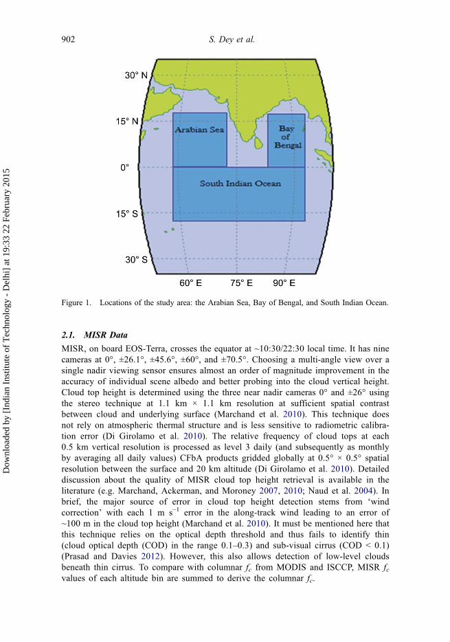
Figure 3 shows the inter-comparison between fc from MISR (fc,MISR) and MODIS(fc,MODIS) over the three oceanic regions. fc,MISR retrieved using the stereo technique andfc,MODIS retrieved using radiometric technique match very well throughout the entireten-year period with a high degree of correlations (correlation coefficients (R) are 0.98,0.96, and 0.77, respectively, for the Arabian Sea, Bay of Bengal, and South Indian Ocean,which are significant at 99% confidence interval). The maximum difference is ~3% overthe Arabian Sea and ~10% over the Bay of Bengal during the winter season and 7–9%

1.0AS:

SIO:BoB:

AS

SIOBoB

0.9

0.8

0.7

0.6

0.5

0.4

0.4 0.5 0.6 0.7 0.8 0.9 1.0fc,MISR

f c,M

OD

IS

0.30.3

fc,MODIS = 1.04 × fc,MISR – 0.03 (R = 0.98)

fc,MODIS = 0.74 × fc,MISR + 0.16 (R = 0.77)fc,MODIS = 0.88 × fc,MISR + 0.13 (R = 0.96)

Figure 3. Correlations between MISR and MODIS-derived fc over the Arabian Sea (AS), Bay ofBengal (BoB), and South Indian Ocean (SIO) for the same period. The correlation coefficients andequations of the best-fit lines are also given. The solid line represents the 1:1 line.

International Journal of Remote Sensing 907

Dow

nloa

ded

by [

Indi

an I

nstit

ute

of T

echn

olog

y -

Del

hi]

at 1

9:33

22

Febr

uary

201

5

during the monsoon season over the South Indian Ocean (Table 1). Several factors maylead to this observed discrepancy. Note that fc is dominated by low clouds (mostlycumulus and stratocumulus) during these periods in the respective regions; hence the‘resolution effect’ may contribute to the discrepancy (Zhao and Di Girolamo 2006). Theview angle geometry of MODIS may be another factor (Maddux, Ackerman, andPlatnick 2010). Different cloud detection techniques and sampling frequency in generat-ing the climatology may also contribute to this discrepancy. For example, a large amountof cirrus clouds are detected by GOCCP and ISCCP over the South Indian Ocean duringthe monsoon season, which may be missed by MISR (Prasad and Davies 2012) anddetected by MODIS due to their respective cloud detection techniques.

Although the sensors show some discrepancy in the absolute values of fc, theseasonality shows appreciable match between all sensors. The seasonality in fc overthese regions is influenced by synoptic meteorology and aerosols. Aerosol opticaldepth, AOD at 558 nm wavelength is obtained from MISR. Quality and applicabilityof MISR AOD in this region were discussed in earlier studies (Dey and DiGirolamo 2010). Large AOD (>0.25) over the Arabian Sea and Bay of Bengal(compared to typical background maritime AOD of <0.15, Smirnov et al. 2009) mayfacilitate cloud formation within a favourable SST range, but fc becomes saturated athigh SST (Gadgil, Joseph, and Joshi 1984; Nair et al. 2011). During the winter season,a large fraction of AOD is absorbing components transported from the Indian land-mass (Kedia et al. 2012), which co-exist with cumulus clouds in the same altituderange (Ramanathan et al. 2007). Cumulus dominates among the low-level clouds inthis region (Bony, Collins, and Fillmore 2000 and also observed in ISCCP climatologyas shown in Figure 5), thus the chance of aerosol–cloud interaction is high (Deyet al. 2011) in this season. Very low aerosol concentration throughout the year overthe South Indian Ocean implies a stronger connection of clouds with meteorology thanwith aerosols. Eastman, Warren, and Hahn (2011) observed that fc does not alwaysshow direct positive correlation with SST because of the competing influences of othermeteorological parameters and aerosols. For example, formation of low clouds (mostlycumulus; Bony, Collins, and Fillmore 2000) may continue over the Arabian Sea andBay of Bengal even during the development of high clouds, probably due to thepresence of larger aerosol concentration. Examining aerosol–cloud-meteorology inter-play is not the focus of this work; however, the contrasting seasonality in observed fcover the Arabian Sea and Bay of Bengal, and the South Indian Ocean signifies theimportance of understanding the climatology of cloud vertical structure in this region.This is required to improve our understanding of aerosol–cloud interaction in allseasons in these regions, since the relative vertical distributions of aerosols and cloudsinfluence aerosol–cloud interaction (Chand et al. 2009).

3.2. Climatology of cloud vertical distribution

MISR-derived mean monthly fc from surface to 20 km altitude at 0.5 km altitude bins isshown in the top panel of Figure 4. Dominance of low-level clouds in the first 3 km overall the three ocean basins is noticeable throughout the year. Mid-to-high-level clouds areobserved to evolve over the Arabian Sea and Bay of Bengal during the monsoon season.On the contrary, the South Indian Ocean shows no seasonality in mid-to-high-levelclouds; instead, there is an increment in the low clouds during the monsoon season(June–September). Mean (±1σ) annual fc of low clouds (summing fc up to 3.5 km altitude)over the Arabian Sea, Bay of Bengal, and South Indian Ocean are 0.34 ± 0.06,

908 S. Dey et al.

Dow

nloa

ded

by [

Indi

an I

nstit

ute

of T

echn

olog

y -

Del

hi]

at 1

9:33

22

Febr

uary

201

5

0.24 ± 0.05, and 0.39 ± 0.11, respectively. Corresponding values for the mid-level (sum offc between 3.5 and 6.5 km) and high clouds (sum of fc above 6.5 km) are 0.08 ± 0.02,0.08 ± 0.01, and 0.16 ± 0.15 and 0.19 ± 0.07, 0.32 ± 0.07, and 0.21 ± 0.10, respectively.Annually, low clouds contribute 57%, 34%, and 55% to fc (in relative terms with respectto columnar fc as reported in Table 1) over the Arabian Sea, Bay of Bengal, and SouthIndian Ocean, respectively, while the corresponding relative contributions of high cloudsare 31%, 46%, and 30%, respectively.

Since ground truth data do not exist in this case to evaluate the MISR statistics, thevertical structure of clouds is examined using GOCCP data (bottom panel of Figure 4).The active sensor can detect multilayer clouds within the same pixel and hence can beconsidered as more accurate than a passive sensor. Our analysis reveals a large amount(fc > 0.3) of high-level clouds at ~14–16 km over the Arabian Sea and Bay of Bengal,especially during the monsoon season. More uniform monthly fc at this altitude range isobserved over the South Indian Ocean relative to the other two regions. In the tropics,large fc at such high altitudes may be attributed to the anvil cirrus (Folkins, Oltmans, and

Figure 4. Mean monthly climatology of fc at 0.5 km altitude bins from the surface to 20 kmaltitude using MISR data for the period March 2000–February 2010 (top panel) and at 0.8 kmaltitude bins from the surface to 19.2 km using GOCCP data for the period June 2006–February2010 (bottom panel) over the Arabian Sea, Bay of Bengal, and South Indian Ocean. Months (in X-axis) are represented by numbers starting from 1 (January) to 12 (December).

International Journal of Remote Sensing 909

Dow

nloa

ded

by [

Indi

an I

nstit

ute

of T

echn

olog

y -

Del

hi]

at 1

9:33

22

Febr

uary

201

5

Thompson 2000), which was confirmed by GOCCP SR profiles. MISR fails to detectcirrus clouds whose optical depth is below 0.3 (Prasad and Davies 2012), while theGOCCP detects clouds with COD > 0.07 (Chepfer et al. 2010). Instead, MISR can seethrough thin cirrus clouds and detect low clouds by the stereo technique. We note thatGOCCP values theoretically represent frequency occurrence of clouds at each altitude bin,which should be kept in mind while carrying out direct comparison between absolutevalues of fc from MISR and GOCCP. During the monsoon season, there is an overallincrease in fc over the Arabian Sea and Bay of Bengal. The increase in fc with height,especially over the Arabian Sea and Bay of Bengal where cloud heights reach 10–15 km,is an indication of the formation of deep convective clouds over these basins. The high-intensity winds transport moisture northwards from the South Indian Ocean leading tolarge convective activity over the Arabian Sea and Bay of Bengal resulting in theformation of convective clouds (Mohanty et al. 2002). However, such seasonal changein cloud vertical structure is not observed over the South Indian Ocean. Monthly varia-tions of fc of low-level clouds are similar for MISR and GOCCP. Slightly high bias inMISR statistics relative to GOCCP may be attributed to the ‘clear conservative’ cloudmask approach of MISR (Zhao and Di Girolamo 2006), which detects any pixel ascompletely cloudy even if it is partially filled by clouds. Hence, this approach over-estimates fc in the tropical regions dominated by small cumulus clouds (e.g. Jones, DiGirolamo, and Zhao 2012). Low bias in low-level cloudiness in GOCCP data may alsoresult from the masking effect of high clouds, as noted by Konsta, Chepfer, andDufresne (2012). Climatology of cloud vertical structure from MISR for the same periodas of GOCCP does not change the overall conclusion.

To gain further understanding of the multilayer cloud field over the oceans as seen fromGOCCP and MISR statistics, the ISCCP D2 data set is also analysed to derive mean monthlycontributions of each individual cloud type to fc (Figure 5). Climatologically, differences inmean annual fc of low, mid-level, and high clouds from ISCCP and MISR are −9%, 3%, and8%, respectively, over the Arabian Sea. Over the Bay of Bengal, ISCCP- andMISR-retrieved fcof low clouds are similar, while ISSCP overestimates mid-level cloud by 9% and underestimateshigh clouds by 5% relative to MISR. ISCCP underestimates the fc of low, mid-level, and high

Figure 5. Monthly statistics of relative abundance of the individual cloud types from ISCCPover the (a) Arabian Sea, (b) Bay of Bengal, and (c) South Indian Ocean for the period January2000–December 2007. Months (in X-axis) are represented by numbers starting from 1 (January)to 12 (December). ‘Cu’, ‘Sc’, ‘St’, ‘Ac’, ‘As’, ‘Ns’, ‘Ci’, ‘Cs’, and ‘Dc’ represent ‘cumulus’,‘stratocumulus’, ‘stratus’, ‘altocumulus’, ‘altostratus’, ‘nimbostratus’, ‘cirrus’, ‘cirrostratus’, and‘deep convective’ clouds, respectively.

910 S. Dey et al.

Dow

nloa

ded

by [

Indi

an I

nstit

ute

of T

echn

olog

y -

Del

hi]

at 1

9:33

22

Febr

uary

201

5

clouds by 7%, 3%, and 5%, respectively, relative to MISR over the South Indian Ocean. On theother hand, high clouds are found to occur more frequently (similar to GOCCP) than other cloudtypes, with the mean annual values of 65% over the Bay of Bengal, 61% over the Arabian Sea,and 51% over the South Indian Ocean (Figure 5). Cirrus dominates among the high cloudsthroughout the year (as also shown byMeenu et al. (2010)). However, the relative abundance ofdeep convective clouds shows a strong seasonal cycle consistent with the monsoon circulationin this region. Cumulus and altocumulus dominate among the low- and mid-level clouds,respectively, and their relative abundances are higher during the post-monsoon and winterseasons over the Arabian Sea and Bay of Bengal compared to other seasons (Bony, Collins, andFillmore 2000). Reduction in relative abundances of cumulus and stratocumulus clouds in theISCCP data during the monsoon season may be attributed to evolution of deep convectiveclouds. Over the South Indian Ocean, the high clouds in ISCCP data do not show muchvariation seasonally (Figure 5(c)), consistent with the GOCCP data, while the increment in lowclouds (as observed in both MISR and GOCCP data in Figure 4) during June–September isattributed to increase in cumulus and stratocumulus clouds (Figure 5(c)).

Overall, the cloud climatology derived from ISCCP complements the MISR-derivedclimatology. Since cloud is detected by a radiometric technique in the ISCCP data set,low-level clouds are difficult to identify if there is an appreciable amount of high-levelclouds such as cirrus in the same pixel. MISR, on the other hand, uses the calibration-insensitive stereo technique, and thus can detect low clouds beneath thin cirrus. Thus bycombining passive sensors MISR and ISCCP, a multilayer cloud field can be interpretedas seen in the GOCCP data set (active sensor) in this region (Marchand et al. 2010).However, we note that the cloud detection thresholds are different in these data sets. Forexample, sub-visual cirrus may still cause a bias in quantitative comparison betweenISCCP-MISR combined climatology and GOCCP climatology.

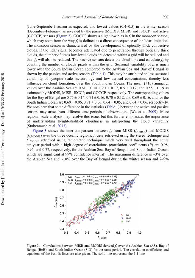
The cloud distributions in day and night-time over these regions are also examinedusing the GOCCP data. The mean seasonal differences in fc vertical structure over theArabian Sea, Bay of Bengal, and South Indian Ocean are shown in Figure 6. The diurnalvariation in day and night-time fc vertical distribution is largest (with fc larger in daytimeby >20%) in the monsoon season below 8 km over all the three regions. The diurnal

–800

5

10

15

(a) (b) (c)20

800–40

Alt

itu

de

(km

)

40 –80 800–40 40 –80 80

MonsoonPre-monsoon

Post-monsoon

Winter

0

Δfc (in %)Δfc (in %)Δfc (in %)

–40 40

Figure 6. Variation of Δfc (difference in night-time fc with respect to daytime fc, in %) with altitudefor four seasons over the (a) Arabian Sea, (b) Bay of Bengal, and (c) South Indian Ocean.

International Journal of Remote Sensing 911

Dow

nloa

ded

by [

Indi

an I

nstit

ute

of T

echn

olog

y -

Del

hi]

at 1

9:33

22

Febr

uary

201

5

variation is almost similar in all the seasons over the Arabian Sea and Bay of Bengal(Figures 6(a) and (b)), while it is larger in the monsoon relative to other seasons over theSouth Indian Ocean above 8 km (Figure 6(c)). Larger fc of low clouds is observed innight-time relative to daytime over the Arabian Sea during the winter season and over theSouth Indian Ocean (between 1 and 3 km altitudes) during all the seasons. The seasonalityin diurnal difference of cloud vertical structure is overall weaker over the South IndianOcean than the other two ocean basins. Throughout the year, night-time fc from passivesensor (MODIS) is observed to be slightly larger relative to the statistics from the active(GOCCP) sensor over the three ocean basins (Table 1).

4. Discussion and Conclusions

In this article, we have presented the climatology of cloud vertical structure over theoceanic regions adjacent to the Indian subcontinent using multi-year passive and activeremote-sensing data. Such multi-sensor comparison helps in understanding the realistic3-D distribution of clouds in view of the strengths and limitations of the sensors and theirdifferent retrieval techniques, as advocated by Stubenrauch et al. (2013). The verticaldistribution of clouds shows strong seasonal variability that may have several implicationsfor the regional climate. Previously, during the Indian Ocean Experiment (Ramanathan,Crutzen, Lelieveld, et al. 2001) and afterwards (e.g. Chylek et al. 2006), strong evidenceof aerosol indirect and semi-direct effect over the North Indian Ocean was reported. Amore recent study (Dey et al. 2011) found evidence of a transition from aerosol indirect tosemi-direct effect on shallow cumulus clouds in this region. The possible influence ofchanges in cumulus cloud cover in response to aerosol forcing on the formation of deepconvection needs to be examined in future. Moreover, the large amount of low clouds(along with larger aerosol loading) in our climatology over the Arabian Sea and Bay ofBengal relative to the South Indian Ocean during the post-monsoon and winter seasonsmay result in a latitudinal asymmetry in SST due to radiative feedback. Whether thisinterpretation holds true, and if yes, whether that influences the monsoon circulation,requires detailed investigation. Many researchers (e.g. Ramanatahn et al. 1989; Rajeevanand Srinivasan 1999) have shown that the net CRF (i.e. balance between SW cooling andLW warming) depends on the cloud vertical distribution. Therefore, the statistics pre-sented here may help in better interpretation of the seasonal variation of net CRF (animportant component of the climate forcing) in this region. These results will further helpin understanding the climate model performances in simulating clouds in this region,which is critical to quantify the cloud radiative feedback (Soden and Vecchi 2011). Forexample, large overestimation of high clouds by the CAM4 model is observed over theBay of Bengal (Zhang et al. 2012). However, for such a comparison, it should be notedthat satellite data are not ground truth; and in fact, considerable discrepancy may exist inobserved vertical structure (although columnar fc may be similar) as reported here. Themulti-sensor statistics presented here will be useful for this purpose.

The major conclusions of the present study are as follows.

(1) fc shows strong seasonal variability over the Arabian Sea and Bay of Bengal withthe highest values (>0.7) during June–July and the lowest values (0.3–0.4) duringFebruary–March. It remains greater than 0.6 throughout the year over the SouthIndian Ocean without much seasonal variability as shown by both passive andactive sensors. This may be attributed to lack of development of convective

912 S. Dey et al.

Dow

nloa

ded

by [

Indi

an I

nstit

ute

of T

echn

olog

y -

Del

hi]

at 1

9:33

22

Febr

uary

201

5

clouds during June–September as opposed to other seasons, as observed in theArabian Sea and Bay of Bengal.

(2) The true cloud vertical structure is better resolved by active sensors (such asGOCCP). MISR detects low clouds beneath thin cirrus using the stereo technique,but underestimates cirrus clouds with respect to GOCCP. ISCCP detects thin cirrususing a radiometric technique, but fails to detect low clouds beneath them. Thus, acombination of passive remote-sensing data from MISR and ISCCP qualitativelycomplements the cloud vertical structure as seen by GOCCP in this region.

(3) Low clouds (mostly cumulus and stratocumulus) increase, while cirrus decreasesover the South Indian Ocean during the northern hemispheric summer monsoonseason. On the other hand, the relative contribution of high clouds (mostlycirrostratus and deep convective clouds) increases over the Arabian Sea andBay of Bengal (larger increase over the Bay of Bengal relative to the ArabianSea) during the monsoon season. Annually, cumulus, altocumulus, and cirrusdominate the low, mid-level, and high clouds, respectively, in all the three regionswith strong seasonal cycle.

(4) Diurnal variation (day vs. night comparison) in fc vertical structure is similar in allfour seasons over the South Indian Ocean, while it is larger in the monsoonseason over the Arabian Sea and Bay of Bengal. During the monsoon, fc duringdaytime below 8 km altitude is larger (by >40%) than that in night-time over theseregions.

(5) The multi-sensor statistics presented here suggest that climate model perfor-mances in simulating cloud vertical structure in this region should not be eval-uated against one particular passive sensor. Even for an active sensor, there maybe a low bias in ‘low cloud’ if optically thick clouds exist aloft.

AcknowledgementsWe acknowledge the comments from two anonymous reviewers that helped in improving the earlierversion of the manuscript.

FundingThis research is supported by the Ministry of Earth Sciences, Government of India under the CTCZprogramme (MoES/CTCZ/16/28/10) through a research grant operational at IIT Delhi (IITD/IRD/RP02479). MISR, MODIS, ISCCP and CERES data are obtained from the NASA Langley ResearchCenter and GOCCP data are obtained from LMD/IPSL (http://climserv.ipsl.polytechnique.fr/cfmip-obs/Calipso_goccp.html).

ReferencesAckerman, S., K. Strabala, P. Menzel, R. Frey, C. Moeller, L. Gumley, B. Baum, S. W. Seeman, and

H. Zhang. 2002. Discriminating Clear-Sky from Cloud with MODIS Algorithm TheoreticalBasis Documents (MOD35), MODIS Documentation. http://modis.gsfc.nasa.gov/data/atbd/atbd_mod06.pdf

Altaratz, O., I. Koren, L. A. Remer, and E. Hirsch. 2014. “Review: Cloud Invigoration by Aerosols-Coupling between Microphysics and Dynamics.” Atmospheric Research 140–141: 38–60.doi:10.1016/j.atmosres.2014.01.009.

Anselmo, T., R. Cliton, W. Hunt, K.-P. Lee, T. Murray, K. Powell, S. D. Rodier, M. Vaughan,O. Chomette, M. Viollier, O. Hagolle, A. Lifermann, A. Garnier, J. Pelon, J. C. Currey, M Pitts,

International Journal of Remote Sensing 913

Dow

nloa

ded

by [

Indi

an I

nstit

ute

of T

echn

olog

y -

Del

hi]

at 1

9:33

22

Febr

uary

201

5

and D.Winker. 2007.Cloud-Aerosol LIDAR Infrared Pathfinder Satellite Observations (CALIPSO)Data Products Catalog. http://csyotc.cira.colostate.edu/documentation/CALIOP/CALIPSO_DPC_Rev2x4.pdf

Bony, S., W. D. Collins, and D. Fillmore. 2000. “Indian Ocean Low Clouds during the WinterMonsoon.” Journal of Climate 13: 2028–2043. doi:10.1175/1520-0442(2000)013<2028:IOLCDT>2.0.CO;2.

Chand, D., R. Wood, T. L. Anderson, S. K. Satheesh, and R. J. Charlson. 2009. “Satellite-DerivedDirect Radiative Effect of Aerosols Dependent on Cloud Cover.” Nature Geoscience 2:181–184. doi:10.1038/ngeo437.

Chepfer, H., S. Bony, D. Winker, G. Cesana, J. L. Dufresne, P. Minnis, C. J. Stubenrauch, andS. Zeng. 2010. “The GCM Oriented CALIPSO Cloud Product (CALIPSO-GOCCP).” Journalof Geophysical Research 115: D00H16. doi:10.1029/2009JD012251.

Chylek, P., M. K. Dubey, U. Lohmann, V. Ramanathan, Y. J. Kaufman, G. Lesins, J. Hudson, G.Altmann, and S. Olsen. 2006. “Aerosol Indirect Effect over the Indian Ocean.” GeophysicalResearch Letters 33: L06806. doi:10.1029/2005GL025397.

Dash, S. K., M. A. Kulkarni, U. C. Mohanty, and K. Prasad. 2009. “Changes in the Characteristicsof Rain Events in India.” Journal of Geophysical Research 114 (D10): D10109. doi:10.1029/2008JD010572.

Dey, S., and L. Di Girolamo. 2010. “A Climatology of Aerosol Optical and MicrophysicalProperties over the Indian Subcontinent from 9 Years (2000-2008) of Multiangle ImagingSpectroradiometer (MISR) Data.” Journal of Geophysical Research 115: D15204.doi:10.1029/2009JD013395.

Dey, S., L. Di Girolamo, G. Zhao, A. L. Jones, and G. M. McFarquhar. 2011. “Satellite-ObservedRelationships between Aerosol and Trade-Wind Cumulus Cloud Properties over the IndianOcean.” Geophysical Research Letters 38: L01804. doi:10.1029/2010GL045588.

Di Girolamo, L., A. Menzies, G. Zhao, K. Mueller, C. Moroney, and D. J. Diner. 2010. “Level 3Cloud Fraction by Altitude Algorithm Theoretical Basis.” JPL D–62358. http://eospso.gsfc.nasa.gov/sites/default/files/atbd/MISR_CFBA_ATBD.pdf

Eastman, R., S. G. Warren, and C. J. Hahn. 2011. “Variations in Cloud Cover and Cloud Types overthe Ocean from Surface Observations, 1954-2008.” Journal of Climate 24: 5914–5934.doi:10.1175/2011JCLI3972.1.

Folkins, I., S. Oltmans, and A. Thompson. 2000. “Tropical Convective Outflow and near SurfaceEquivalent Potential Temperatures.” Geophysical Research Letters 27: 2549–2552. doi:10.1029/2000GL011524.

Gadgil, S., P. V. Joseph, and N. V. Joshi. 1984. “Ocean-Atmosphere Coupling over MonsoonRegions.” Nature 312: 141–143. doi:10.1038/312141a0.

Goren, T., and D. Rosenfeld. 2014. “Decomposing Aerosol Cloud Radiative Effects into CloudCover, Liquid Water Path and Twomey Components in Marine Stratocumulus.” AtmosphericResearch 138: 378–393. doi:10.1016/j.atmosres.2013.12.008.

Goswami, B. N., V. Venugopal, D. Sengupta, M. S. Madhusoodan, and P. K. Xavier. 2006.“Increasing Trend of Extreme Rain Events over India in a Warming Environment.” Science314 (5804): 1442–1445. doi:10.1126/science.1132027.

IPCC (Intergovernmental Panel on Climate Change). 2007. Climate Change 2007: The physicalbasis: contribution of working group I to the Fourth Assessment Report, Chapter 2.

Jin, X., J. Hanesiak, and D. Barber. 2007. “Detecting Cloud Vertical Structures from Radiosondesand MODIS over Arctic First-Year Sea Ice.” Atmospheric Research 83: 64–76. doi:10.1016/j.atmosres.2006.03.003.

Jones, A. L., L. Di Girolamo, and G. Zhao. 2012. “Reducing the Resolution Bias in Cloud Fractionfrom Satellite Derived Clear-Conservative Cloud Masks.” Journal of Geophysical Research117: D12201. doi:10.1029/2011JD017195.

Kedia, S., S. Ramachandran, T. A. Rajesh, and R. Srivastava. 2012. “Aerosol Absorption over Bayof Bengal during Winter: Variability and Sources.” Atmospheric Environment 54: 738–745.doi:10.1016/j.atmosenv.2011.12.047.

Klein, S. A., Y. Zhang, M. D. Zelinka, R. Pincus, J. Boyle, and P. J. Gleckler. 2013. “Are ClimateModel Simulations of Clouds Improving? An Evaluation Using the ISCCP Simulator.” Journalof Geophysical Research 118 (3): 1329–1342. doi:10.1002/jgrd.50141

Konsta, D., H. Chepfer, and J.-L. Dufresne. 2012. “A Process Oriented Characterization of TropicalOceanic Clouds for Climate Model Evaluation, Based on A Statistical Analysis of Daytime A-

914 S. Dey et al.

Dow

nloa

ded

by [

Indi

an I

nstit

ute

of T

echn

olog

y -

Del

hi]

at 1

9:33

22

Febr

uary

201

5

Train Observations.” Climate Dynamics 39 (9–10): 2091–2108. doi:10.1007/s00382-012-1533-7.

Kühnlein, M., T. Appelhans, B. Thies, A. A. Kokhanovsky, and T. Nauss. 2013. “An Evaluation of aSemi-Analytical Cloud Property Retrieval Using MSG SEVIRI, MODIS and Cloudsat.”Atmospheric Research 122: 111–135. doi:10.1016/j.atmosres.2012.10.029.

Loeb, N., and G. L. Schuster. 2008. “An Observational Study of the Relationship between Cloud,Aerosol and Meteorology in Broken Low-Level Cloud Conditions.” Journal of GeophysicalResearch 113: D14214. doi:10.1029/2007JD009763.

Maddux, B. C., S. A. Ackerman, and S. Platnick. 2010. “Viewing Geometry Dependencies inMODIS Cloud Products.” Journal of Atmospheric and Oceanic Technology 27: 1519–1528.doi:10.1175/2010JTECHA1432.1.

Marchand, R., T. Ackerman, M. Smyth, and W. B. Rossow. 2010. “A Review of Cloud Top Heightand Optical Depth Histograms from MISR,ISCCP, and MODIS.” Journal of GeophysicalResearch 115. doi:10.1029/2009JD013422.

Marchand, R. T., T. P. Ackerman, and C. Moroney. 2007. “An Assessment of Multiangle ImagingSpectroradiometer (MISR) Stereo-Derived Cloud Top Heights and Cloud Top Winds UsingGround-Based Radar, Lidar and Microwave Radiometers.” Journal of Geophysical Research112: D06204. doi:10.2029/2006JD009191.

Meenu, S., K. Rajeev, and K. Paramaeswaran. 2011. “Regional and Vertical Distribution ofSemitransparent Cirrus Clouds over the Tropical Indian Region Derived from CALIPSOData.” Journal of Atmospheric and Solar-Terrestrial Physics 73: 1967–1979.

Meenu, S., K. Rajeev, K. Parameswaran, and A. K. M. Nair. 2010. “Regional Distribution of DeepClouds and Cloud Top Altitudes over the Indian Subcontinent and the Surrounding Oceans.”Journal of Geophysical Research 115: D5. doi:10.1029/2009JD11802.

Mohanty, U. C., R. Bhatla, P. V. S. Raju, O. P. Madan, and A. Sarkar. 2002. “Meteorological FieldsVariability over the Indian Seas in Pre and Summer Monsoon Months during Extreme MonsoonSeasons.” Earth and Planetary Science 111 (3): 365–378.

Nair, A. K. M., K. Rajeev, S. Sijikumar, and S. Meenu. 2011. “Characteristics of a Persistent ‘Poolof Inhibited Cloudiness’ and Its Genesis over the Bay of Bengal Associated with the AsianSummer Monsoon.” Annals of Geophysics 29: 1247–1252. doi:10.5194/angeo-29-1247-2011.

Naud, C., J. P. Muller, M. Haeffelin, Y. Morille, and A. Delaval. 2004. “Assessment of MISR andMODIS Cloud Top Heights through Inter-Comparison with a Back-Scattering Lidar at SIRTA.”Geophysical Research Letters 31 (4): L04114. doi:10.1029/2003GL018976.

Patil, S. D., and R. K. Yadav. 2005. “Large-Scale Changes in the Cloud Radiative Forcing over theIndian Region.” Atmospheric Environment 39 (26): 4609–4618. doi:10.1016/j.atmosenv.2005.03.051.

Platnick, S., M. D. King, S. A. Ackerman, W. P. Menzel, B. A. Baum, J. C. Riedi, and R. A. Frey.2003. “The MODIS Cloud Products: Algorithms and Examples from Terra.” IEEE Transactionson Geoscience and Remote Sensing 41 (2): 459–473.

Prasad, A. A., and R. Davies. 2012. “Detecting Tropical Thin Cirrus Using Multiangle ImagingSpectroradiometer’s Oblique Cameras and Modeled Outgoing Longwave Radiation.” Journal ofGeophysical Research 117 (D6): D06208.

Probst, P., R. Rizzi, E. Tosi, V. Lucarini, and T. Maestri. 2012. “Total Cloud Cover from SatelliteObservations and Climate Models.” Atmospheric Research 107: 161–170.

Rajeevan, M., and J. Srinivasan. 1999. “Net Cloud Radiative Forcing at the Top of Atmosphere inthe Asian Monsoon Region.” Journal of Climate 13: 650–657.

Ramanathan, V., R. D. Cess, E. F. Harrison, P. Minnis, B. R. Barkstrom, E. Ahmad, and D.Hartmann. 1989. “Cloud Radiative Forcing and Climate: Results from the Earth RadiationBudget Experiment.” Science 243: 57–63.

Ramanathan, V., P. J. Crutzen, J. T. Kiehl, and D. Rosenfeld. 2001. “Aerosols, Climate and theHydrological Cycle.” Science 294: 2119–2124.

Ramanathan, V., P. J. Crutzen, J. Lelieveld, A. P. Mitra, D. Althausen, J. Anderson, M. O. Andreae,W. Cantrell, G. R. Cass, C. E. Chung, A. D. Clarke, J. A. Coakley, W. D. Collins, W. C. Conant,F. Dulac, J. Heintzenberg, A. J. Heymsfield, B. Holben, S. Howell, J. Hudson, A. Jayaraman, J.T. Kiehl, T. N. Krishnamurti, D. Lubin, G. McFarquhar, T. Novakov, J. A. Ogren, I. A.Podgorny, K. Prather, K. Priestley, J. M. Prospero, P. K. Quinn, K. Rajeev, P. Rasch, S.Rupert, R. Sadourny, S. K. Satheesh, G. E. Shaw, P. Sheridan, and F. P. J. Valero. 2001.

International Journal of Remote Sensing 915

Dow

nloa

ded

by [

Indi

an I

nstit

ute

of T

echn

olog

y -

Del

hi]

at 1

9:33

22

Febr

uary

201

5

“Indian Ocean Experiment: An Integrated Analysis of the Climate Forcing and Effects of theGreat Indo-Asian Haze.” Journal of Geophysical Research 106. doi:10.1029/2001JD900133.

Ramanathan, V., M. V. Ramana, G. Roberts, D. Kim, C. E. Corrigan, C. E. Chung, and D. Winker.2007. “Warming Trends in Asia Amplified by Brown Cloud Solar Absorption.” Nature 448:575–578.

Randall, D., S. Krueger, C. Bretherton, J. Curry, P. Duynkerke, M. Moncrieff, B. Ryan, D. Starr, M.Miller, W. Rossow, G. Tselioudis, and B. Wielick. 2003. “Confronting Models with Data, theGEWEX Cloud Systems Study.” Bulletin of the American Meteorological Society 84: 455–469.

Rossow, W. B., and R. A. Schiffer. 1999. “Advances in Understanding Clouds from ISCCP.”Bulletin of the American Meteorological Society 80: 2261–2288.

Sathiyamoorthy, V., P. K. Pal, and P. C. Joshi. 2011. “Influence of the Upper-Tropospheric WindShear upon Cloud Radiative Forcing in the Asian Monsoon Region.” Journal of Climate 17(14): 2725–2735.

Smirnov, A., B. N. Holben, I. Slutsker, D. M. Giles, C. R. McClain, T. F. Eck, S. M. Sakerin, A.Macke, P. Croot, G. Zibordi, P. K. Quinn, J. Sciare, S. Kinne, M. Harvey, T. J. Smyth, S. Piketh,T. Zielinski, A. Proshutinsky, J. I. Goes, N. B. Nelson, P. Larouche, V. F. Radionov, P. Goloub,K. Krishna Moorthy, R. Matarrese, E. J. Robertson, and F. Jourdin. 2009. “Maritime AerosolNetwork as a Component of Aerosol Robotic Network.” Journal of Geophysical Research 114:D06204.

Soden, B. J., and G. A. Vecchi. 2011. “The Vertical Distribution of Cloud Feedback in CoupledOcean-Atmosphere Models.” Geophysical Research Letters 38: L12704. doi:10.1029/2011GL047632.

Stubenrauch, C. J., W. B. Rossow, S. Kinne, S. Ackerman, G. Cesana, H. Chepfer, L. Di Girolamo,B. Getzewich, A. Guignard, A. Heidinger, B. C. Maddux, W. P. Menzel, P. Minnis, C. Pearl, S.Platnick, C. Poulsen, J. Riedi, S. Sun-Mack, A. Walther, D. Winker, S. Zeng, and G. Zhao.2013. “Assessment of Global Cloud Datasets from Satellites: Project and Database Initiated bythe GEWEX Radiation Panel.” Bulletin of the American Meteorological Society 94: 1031–1049.

Verlinden, K. L., D. W. J. Thompson, and G. L. Stephens. 2011. “The Three-DimensionalDistribution of Clouds over the Southern Hemisphere High Latitudes.” Journal of Climate24: 5799–5811.

Wonsick, M. M., R. T. Pinker, and Y. Govaerts. 2009. “Cloud Variability over the Indian Monsoonas Observed from Satellites.” Journal of Applied Meteorology and Climatology 48: 1803–1821.

Wu, D. L., S. A. Ackerman, R. Davies, D. J. Diner, M. J. Garay, B. H. Kahn, B. C. Maddux, C. M.Moroney, G. L. Stephens, J. P. Veefkind, and M. A. Vaughan. 2009. “Vertical Distributions andRelationships of Cloud Occurrence Frequency as Observed by MISR, AIRS, MODIS, OMI,CALIPSO and Cloudsat.” Geophysical Research Letters 36: L09821. doi:10.1029/2009GL037464.

Wylie, D. P., W. P. Menzel, and K. I. Strabala. 1994. “Four Years of Global Cirrus Cloud StatisticsUsing HIRS.” Journal of Climate 7: 1972–1986.

Xi, B., X. Dong, P. Minnis, and M. M. Khaiyer. 2010. “A 10 Year Climatology of Cloud Fractionand Vertical Distribution Derived from Both Surface and GOES Observations over the DOEARM SPG Site.” Journal of Geophysical Research 115: D12124. doi:10.1029/2009JD012800.

Zhang M. H., W. Y. Lin, S. A. Klein, J. T. Bacmeister, S. Bony, R. T. Cederwall, A. D. Del Genio, J.J. Hack, N. G. Loeb, U. Lohmann, P. Minnis, I. Musat, R. Pincus, P. Stier, M. J. Suarez, M. J.Webb, J. B. Wu, S. C. Xie, M.-S. Yao, and J. H. Zhang. 2005. “Comparing Cloud and TheirSeasonal Variation in Ten Atmospheric General Circulation Models with SatelliteMeasurements.” Journal of Geophysical Research 110: D15S02. doi:10.1029/2004JD005021.

Zhang, Y., S. Xie, C. Covey, D. D. Lucas, P. Gleckler, S. A. Klein, J. Tannahill, C. Doutriaux, andR. Klein. 2012. “Regional Assessment of the Parameter-Dependent Performance of CAM4 inSimulating Tropical Clouds.” Geophysical Research Letters 39: L14708.

Zhao, G., and L. Di Girolamo. 2006. “Cloud Fraction Errors for Trade Wind Cumuli from EOS-TerraInstruments.” Geophysical Research Letters 33: L20802. doi:10.1029/2006GL027088.

916 S. Dey et al.

Dow

nloa

ded

by [

Indi

an I

nstit

ute

of T

echn

olog

y -

Del

hi]

at 1

9:33

22

Febr

uary

201

5