Sensing, Navigation and Reasoning Technologiesfor the DARPA Urban Challenge

Joel W. Burdick Noel duToit Andrew Howard Christian LoomanJeremy Ma Richard M. Murray! Tichakorn Wongpiromsarn

California Institute of Technology/Jet Propulsion Laboratory

DARPA Urban Challenge Final Report31 December 2007, Team Caltech

Approved for public release; distribution is unlimited.

AbstractThis report describes Team Caltech’s technical approach and results for the 2007 DARPA UrbanChallenge. Our primary technical thrusts were in three areas: (1) mission and contingency manage-ment for autonomous systems; (2) distributed sensor fusion, mapping and situational awareness;and (3) optimization-based guidance, navigation and control. Our autonomous vehicle, Alice,demonstrated new capabiliites in each of these areas and drove approximate 300 autonomous milesin preparation for the race. The vehicle completed 2 of the 3 qualification tests, but did not ulti-mately qualify for the race due to poor performance in the merging tests at the National QualifyingEvent.

1 Introduction and OverviewTeam Caltech was formed in February of 2003 with the goal of designing a vehicle that couldcompete in the 2004 DARPA Grand Challenge. Our 2004 vehicle, Bob, completed the qualifica-tion course and traveled approximately 1.3 miles of the 142-mile 2004 course. In 2004-05, TeamCaltech developed a new vehicle—Alice, shown in Figure 1—to participate in the 2005 DARPAGrand Challenge. Alice utilized a highly networked control system architecture to provide highperformance, autonomous driving in unknown environments. The system successfully completedseveral runs in the National Qualifying Event, but encountered a combination of sensing and con-trol issues in the Grand Challenge Event that led to a critical failure after traversing approximately8 miles.

As part of the 2007 Urban Challenge, Team Caltech developed new technology for Alice inthree key areas: (1) mission and contingency management for autonomous systems; (2) distributedsensor fusion, mapping and situational awareness; and (3) optimization-based guidance, navigationand control. This section provides a summary of the capabilities of our vehicle and describes theframework that we used the 2007 Urban Challenge.

!Corresponding author: murray@cds.caltech.edu

Final Report, 2007 DARPA Urban Challengehttp://www.cds.caltech.edu/~murray/papers/bur+07-dgc.html

Team Caltech

Figure 1: Alice, Team Caltech’s entry in the 2007 Urban Challenge.

For the 2007 Urban Challenge, we built on the basic architecture that was deployed by Caltechin the 2005 race, but provided significant extensions and major additions that allowed operationin the more complicated (and uncertain) urban driving environment. Our primary approach in thedesert competition was to construct an elevation map of the terrain sounding the vehicle and thenconvert this map into a cost function that could be used to plan a high speed path through theenvironment. A supervisory controller provided contingency management by identifying selectedsituations (such as loss of GPS or lack of forward progress) and implementing tactics to overcomethese situations.

To allow driving in urban environments, several new challenges had to be addressed. Roadlocation had to be determined based on lane and road features, static and moving obstacles mustbe avoided, and intersections must be successfully navigated. We chose a deliberative planningarchitecture, in which a representation of the environment was built up through sensor data andmotion planning was done using this representation. A significant issue was the need to reasonabout traffic situations in which we interact with other vehicles or have inconsistent data about thelocal environment or traffic state.

The following technical accomplishments were achieved as part of this program:

1. A highly distributed, information-rich sensory system was developed that allowed real-timeprocessing of large amounts of raw data to obtain information required for driving in urbanenvironments. The distributed nature of our system allowed easy integration of new sensors,but required sensor fusion in both time and space across a distributed set of processes.

2. A hierarchical planner was developed for driving in urban environments that allowed com-plex interactions with other vehicles, including following, passing and queuing operations.A rail-based planner was used to allow rapid evaluation of maneuvers and choice of pathsthat optimized competing objectives while insuring safe operation in the presence of othervehicles and static obstacles.

3. A canonical software structure was developed for use in the planning stack to insure that con-tingencies could be handled and that the vehicle would continue to make forward progress

2

Team Caltech

towards its goals for as long as possible. The combination of a directive/response mech-anism for intermodule communication and fault-handling algorithms provide a rich set ofbehaviors in complex driving situations.

The features of our system were demonstrated in approximately 300 miles of testing performed inthe months before the race, including the first known interaction between two autonomous vehicles(with MIT, in joint testing at the El Toro Marine Corps Air Station).

A number of shortfalls in our approach led to our vehicle being disqualified for the final race:

1. Inconsistencies in the methods by which obstacles were handled that led to incorrect behav-ior in situations with tight obstacles;

2. Inadequate testing of low-level feature extraction of stop lines and the corresponding fusioninto the existing map;

3. Complex logic for handling intersections and obstacles that was difficult to modify and testin the qualification event.

Despite these limitations in our design, Alice was able to perform well on 2 out of the 3 test areasat the NQE, demonstrating the ability to handle a variety of complex traffic situations.

This report is organized as follows: Section 2 provides a high level overview of our approachand system architecture, including a description of some of the key infrastructure used throughoutthe problems. Sections 3–5 describes in the main software subsystems in more detail, includingmore detailed descriptions of the algorithms used for specific tasks. A description of the primarysoftware modules used in the system is included. Section 6 provides a summary of the results fromthe site visit, testing leading up to the NQE and the team’s performance in each of the NQE tests.Finally, Section 7 summarizes the main accomplishments of the project, captures lessons learnedand describes potential transition opportunities. Appendix A provides a listing of additional mod-ules that are referenced in the report along with a short description of the module.

2 System Overview

2.1 System ArchitectureA key element of our system is the use of a networked control systems (NCS) architecture thatwe developed in the first two grand challenge competitions. Building on the open source Spreadgroup communications protocol, we have developed a modular software architecture that providesinter-computer communications between sets of linked processes [1]. This approach allows theuse of significant amounts of distributed computing for sensor processing and optimization-basedplanning, as well as providing a very flexible backbone for building autonomous systems andfault tolerant computing systems. This architecture also allows us to include new components ina flexible way, including modules that make use of planning and sensing modules from the JetPropulsion Laboratory (JPL).

3

Team Caltech

ME(2)Obst

MovingVehicles

VehiclePrediction

module startupF1

LADAR

Stereo

RADAR

Sens

net

mapv’r

Fusion/Classify

health monitor

PTU atten’n

follow

adrive

mplanner F3

asim

trafsim

astate

ROA

Cabin Power Vehicle Estop ActuatorsMountsField Ops

Line

Road

F2F5F4

F6

Mapper

F10

F7

F8

F9

Plan

ner

Update mapFSMPlan pathCompute vel

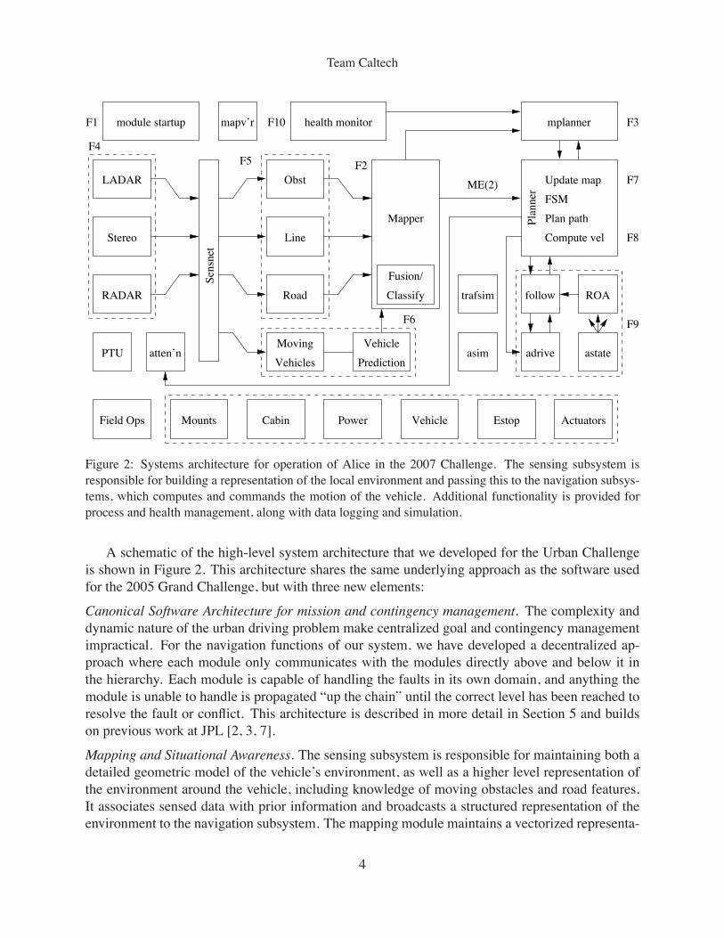
Figure 2: Systems architecture for operation of Alice in the 2007 Challenge. The sensing subsystem isresponsible for building a representation of the local environment and passing this to the navigation subsys-tems, which computes and commands the motion of the vehicle. Additional functionality is provided forprocess and health management, along with data logging and simulation.

A schematic of the high-level system architecture that we developed for the Urban Challengeis shown in Figure 2. This architecture shares the same underlying approach as the software usedfor the 2005 Grand Challenge, but with three new elements:

Canonical Software Architecture for mission and contingency management. The complexity anddynamic nature of the urban driving problem make centralized goal and contingency managementimpractical. For the navigation functions of our system, we have developed a decentralized ap-proach where each module only communicates with the modules directly above and below it inthe hierarchy. Each module is capable of handling the faults in its own domain, and anything themodule is unable to handle is propagated “up the chain” until the correct level has been reached toresolve the fault or conflict. This architecture is described in more detail in Section 5 and buildson previous work at JPL [2, 3, 7].

Mapping and Situational Awareness. The sensing subsystem is responsible for maintaining both adetailed geometric model of the vehicle’s environment, as well as a higher level representation ofthe environment around the vehicle, including knowledge of moving obstacles and road features.It associates sensed data with prior information and broadcasts a structured representation of theenvironment to the navigation subsystem. The mapping module maintains a vectorized representa-

4

Team Caltech

tion of static and dynamic sensed obstacles, as well as detected lane lines, stop lines and waypoints.The map uses a 2.5 dimensional representation where the world is projected into a flat 2D plane,but individual elements may have some non-zero height. Each sensed element is tracked over timeand when multiple sensors overlap in field of view, the elements are fused to improve robustness tofalse positives as well as overall accuracy. These methods are described in more detail in Section 3.

Route, Traffic and Path Planning. The planning subsystem determines desired motion of the sys-tem, taking into account the current route network and mission goals, traffic patterns and drivingrules and terrain features (including static obstacles). This subsystem is also responsible for pre-dicting motion of moving obstacles, based on sensed data and road information, and for imple-menting defensive driving techniques. The planning problem is divided into three subproblems(route, traffic, and path planning) and implemented in separate modules. This decomposition waswell-suited to implementation by a large development team since modules could be developed andtested using earlier revisions of the code base as well as using simulation environments. Additionaldetails are provided in Section 4.

2.2 Project ModificationsThe overall approach described in our original proposal and technical paper were maintainedthrough the development cycle. After the site visit, the planning subsystem was modified due toproblems in getting our original optimization-based software to run in real-time. Specifically, theNURBS-based dynamic planner described in the technical paper was replaced by a graph search-based planner. At a high level, these two planner both generated a path that obeyed the currentlyactive traffic rules, avoided all static and dynamic obstacles, and optimized a cost function basedon road features and the local environment. However, the rail-based planner separated the spatial(path) planning problem from the temporal (velocity) planning problem and made use of a partiallypre-computed graph to allow a coarse plan to be developed very quickly. The revised planner isdescribed in more detail in Section 4.2.

In addition, the internal structure of the planning stack was reorganized to streamline the pro-cessing of information and minimize the number of internal states of the planner. The probabilisticfinite state machine used to estimate traffic state was replaced with a simpler finite state machineimplementation.

Other differences from the technical paper include:

• The final sensor suite included two RADAR units mounted on separate pan-tilt units and noIR camera. This approach was used to allow long-range detection of vehicles at intersection(one RADAR was pointed in each direction down the road).

• Rather than using separate obstacles maps from individual LADARs and fusing them, asingle algorithm that processed all LADAR data was developed. This approach improvedrobustness of the system, especially differentiating static and moving vehicles.

• The sensor fusion algorithms for certain objects were moved from the map object directlyinto the planner. This allowed better spatio-temporal fusion and persistence of intermittentobjects.

5

Team Caltech

Figure 3: Screen shots from SensViewer (left) and MapViewer (right).

3 Sensing SubsystemThe sensing subsystem was developed from approaches for sensing, mapping and situationalawareness that built off past work at Caltech/JPL. As can be seen from Figure 2, there are es-sentially three layers to the sensing subsystem. The flow of sensory data begins with the feedersin function block F4 and travels (via the SensNet interface) to the perceptors in function block F5.The perceptors then apply their respective perception algorithms and pass the perceived featuresto the map in function block F2, where fusion and classification is performed. In short, we canclassify these layers as follows:

Sensing Hardware & Feeders: This layer consists of the low-level drivers and feeders that makethe raw sensed data available to the perception algorithms. Each sensor is identified by a uniquesensor-ID to keep things organized and allows the ease of incorporating new sensors as they getintroduced.

Perception Software: This layer consists of the perception algorithms that take in the raw senseddata from the feeders and apply detection and tracking to extracted features from the data; suchfeatures include lines on the road, static obstacles, traversable hazards and moving vehicles.

Fused Map: This final layer consists of the vectorized representation of the world which we referto as the “map”. The map receives all the detected and tracked features that have been extracted atthe perceptor level and fuses them to form a vectorized map database which is used by the planners.

Figure 3 contains screen shots illustrating the features of the sensing systems. The left figuresshows the direct data from the various sensors represented in a 3D view. Images from the short andmedium range cameras are shown at the top of the figure, and the LADAR, RADAR and stereoobstacle data are shown below. This information is processed by the perceptors, resulting in thefused data shown in the right figure. In this representation, obstacles are classified as static ormoving. Lane data (not shown) is also stored in the map.

6

Team Caltech

The following subsections address each layer of the sensing subsystem, with detailed descrip-tions of associated modules that were respectively used during the qualifying events at the NQE.

3.1 Sensing Hardware & Feeders

SensNet. Data from feeders is transmitted to perceptors using a specialized high-bandwidth, low-latency communication package called SensNet. SensNet’s connection model is many-to-many,such that each feeder can supply multiple perceptors and each perceptor can subscribe to multi-ple feeders. Perceptors can therefore draw on any combination of sensors and/or sensor modal-ities to accomplish their task (e.g., a road perceptor can use both forward-facing cameras andforward-facing LADARs). SensNet will also choose an appropriate interprocess communicationmethod based on the location of the communicating modules. For modules on the same phys-ical machine, the method is shared memory; for modules on different machines, the method isSpread/TCP/Ethernet.

LADAR Feeder. The LADAR-feeder module works by interfacing with a variety of laser rangefinders using existing drivers which had been written (or rewritten) from previous races. For thisparticular race, the laser range finders we had used were the SICK LMS-221, the SICK LMS-291, and the RIEGL LMS-Q120. Depending on the sensor-ID given (specified as a command lineargument to the module), this module calls the correct driver to interface with the desired scannerand broadcasts the resulting scan measurements across SensNet. The range scan is referenced inthe sensor frame yet tagged with the vehicle state and appropriate matrix transforms to allow forflexibility in transforming the range points into any desired frame (i.e. sensor, local, vehicle).

Stereo Feeder. The stereo-feeder module works by reading in the raw images from all fourcameras (two sets of stereo-camera pairs: one long-baseline and one medium-baseline). With theknown baselines between cameras in a given stereo-camera pair, a disparity and range value iscalculated for all corresponding pixels in both images using JPL stereo software. Finally, the rawimage with disparity and range values is then sent across SensNet to all listening modules.

RADAR Feeder. The radar-feeder module works by interfacing with a TRW AC20 AutocruiseRADAR unit and publishing the data to SensNet. The AC20 can report up to ten “targets” (in-termittent, single-cycle returns) and ten “tracks”—internally tracked objects—at a refresh rate of26 Hz. The internal tracking is fairly accurate, and when supplied with the vehicle’s yaw rate andvelocity, can compensate for its own motion. It filters out stationary returns, making it ideal for acar perceptor.

PTU Feeder. The Pan-Tilt-Unit (PTU) feeder is the controlling software that receives panningand tilting commands for one of two pan-tilt unit devices on the vehicle: the Amtec Robotics Pow-ercube pan-tilt-unit or the Directed Perception PTU-D46-17. The panning and tilting commandscan be specified in one of two ways:

• specifying pan-tilt angles in the PTU reference frame;• specifying a point in the local-frame such that the line-of-site vector of the pan-tilt unit

intersects that point (i.e. such that the pan-tilt-unit is looking at that point in space).

7

Team Caltech

There are elements of this module that make it work like a feeder and elements that make it worklike an actuator. The module is a feeder in the sense that it continually broadcasts its pan and tiltangles across SensNet. It is an actuator in the sense that it listens for messages that command amovement and executes those commands.

3.2 Perception Software

Line/Road Perceptor. There were essentially two line perceptors that were written for theDARPA Urban Challenge. The first line perceptor was identified as the “Line Perceptor” mod-ule and by an abuse of notation, the second line perceptor module was identified as the “RoadPerceptor” module. A description of each module is provided below.

The Line Perceptor takes in raw sensory image data from the stereo camera feeders and appliesa perception algorithm that filters out line features (e.g. stop lines, lane lines, and parking-lanelines) and sends them to the Map module. The details of the algorithm are outlined in the followingsteps:

1. The image is transformed into Inverse Perspective Mapping view (IPM) given the cameraexternal calibration parameters. IPM works by assuming the road is a flat plane, and usingthe camera intrinsic (focal length and optical center) and extrinsic (pitch angle, yaw angle,and height above ground) parameters to take a top view of the road. This makes the width ofany line uniform and independent of its position in the image, and only dependent on its realwidth in reality. It also removes the perspective effect, so that lines parallel to the opticalaxis will be parallel and vertical.

2. Spatial filtering is then done on the IPM image, using steerable filters, to detect horizontallines (in case of stop lines) or vertical lines (in case of lanes). The filters are Gaussian inone direction and second derivative of Gaussian in the perpendicular direction, which is bestsuited to detect light line on dark background.

3. Thresholding is then performed on the image to extract the highest values from the filteredimage. This is done be selecting the highest kth percentile of values from the image.

4. Line grouping is done on the thresholded image, using either of:

• Hough transform: for detecting straight lines;• RANSAC lines: for detecting straight lines;• Histograms: a simplified version of Hough transform for detecting only horizontal and

vertical lines;• RANSAC splines: for fitting splines to thresholded image.

The Hough transform approach is the default mode of operation which provides flexibilityin detecting lines of any orientation or position in the image. The orientations are searchedbetween ± 10 degrees of horizontal or vertical, which allows for lane features that are notorthogonally aligned to the vehicle to be detected.

8

Team Caltech

5. Validation and localization is then performed on detected lines and splines to better fit theimage and to get end-points for the lines before finally sending to the Map module. Weisolate the pixels belonging to the detected stop line using Bresenham’s line drawing algo-rithm, and then convolve a smoothed version of the pixel values on the line with two kernelsrepresenting a rising and a falling edge, and getting the points of maximum response. Thedetected lines and splines are transformed back to the original image plane, and then to thelocal frame, which are then sent to the Map module.

The Road Perceptor module has a very similar architecture to the Line Perceptor module de-scribed above and can be briefly summarized in the following seven steps:

1. The first step loads images from the left camera taken from the stereo-feeder modules, whichcan either be from the middle baseline pair or the longer baseline pair. The default settingwas to use the middle baseline pair.

2. The next step applies some pre-processing to enhance the loaded images (e.g. removing thehood of the vehicle from the bottom of the image and color separation for white vs. yellowlines).

3. Edge detection is next applied to the enhanced image which is done by applying an operatorthat extracts the main road hints in the form of edges or contours from the images.

4. Line extraction is then applied to the detected edges to extract candidate lines using theprobabilistic Hough transform.

5. Line association then classifies the extracted lines as good lines or bad lines according totheir color, geometrical properties, and relation with other lines.

6. Perspective Translation is then applied to the valid lines in much the same way described forthe Line Perceptor module.

7. Line output is then executed on the translated lines, which are parameterized and broken intopoints then sent to the Map module.

Additional details on this algorithm are given in [6].

LADAR-BasedObstacle Perceptor. The LADAR-based Obstacle Perceptor has two main threads,preprocessing and tracking. The preprocessing thread is in charge of retrieving the latest laser rangedata (from all available LADARs) from the SensNet module and transforming it to the local frame.Once in the local frame, the data is then incorporated into a couple of occupancy grid maps:

• Static Map The static map is a map of free and occupied space represented by cells. All cellsare first initialized to a negative value and when the actual returns are read in, correspondingcells are given a positive value. This map is used for grouping noisy obstacles like bushesand berms in an easy manner.

• Road Map The road map contains a map of large smooth surfaces likely to be road (storedas elevation data).

9

Team Caltech

• Groundstrike Map The “groundstrike” map has cumulative information about what areasare likely to be LADAR scans generated by striking the ground. The data in this map isgenerated primarily from the elevation data gathered from the sweeping pan-tilt unit.

The second thread, the tracking thread, relies on discrete tracking of segments using a vec-torized representation instead of a grid-based representation. For each LADAR, every incomingscan is segmented based on discontinuities (as a function of distance) and evaluated as a potential“groundstrike” based on the groundstrike probabilities of its constituent points. If a segment is ac-cepted, it is associated with existing tracked segments or a new track is created. The function of thetracking is primarily to detect dynamic obstacles, since everything not dynamic is treated equiva-lently as static. Thus tracks are weighted by how likely they are to be cars (reflectivity, size, etc).The tracking just uses a standard Kalman filter for the centroid, though extra care is taken wheninitializing tracks to avoid misidentifying changing geometry as a high initial velocity. To combinethe individual LADAR scans, each new set of scans is broken up into clusters of points (based onpoint-point distance), again to merge noisy obstacles into one large blob. For each cluster, thevelocity is computed as the weighted average of each point’s associated segment track, weightedby the status (confidence) of that track. Basic nearest obstacle association is done between scans;this is to maintain a consistent obstacle ID throughout the lifetime of a given obstacle. Dynamicobstacle classification occurs at this level, and is determined by the distance an obstacle has movedfrom its initial position, its velocity, and how long it has been visible. After a certain amount oftime, an obstacle cannot be unclassified as dynamic. A reasonable geometry for each obstacle isthen computed and the data is sent to the Map module.LADAR-Based Curb Perceptor. The ladar-curb-perceptor (LCP) module is intended to detectand track the right side of the road. The “curb” in question need not be an engineered street curb,but rather denotes any sufficiently long, linear cluster of LADAR-visible obstacles that is nearlyaligned with the vehicle’s current direction of travel. This could be a row of bushes or sandbags, aberm, a building facade, or even a ditch. The LCP uses two sensors: the roof-mounted Riegl laserrange finder (the beam which intersects the ground plane "15 m in front of Alice), and the middlefront bumper SICK laser range finder (the sweep plane of which is parallel to the ground). TheRiegl enables the LCP to see obstacles of any height, including negative, but only out to its ground-intersection distance. The SICK sees only obstacles over "1 m high, but out to a much greaterrange. Each scan of the LADARs is laterally filtered for step-edge detection; points that pass areconsidered obstacles which may be part of a curb (this procedure is robust to ground strikes dueto pitching). Obstacle locations are converted to vehicle coordinates for aggregation over time,yielding a 2-D distribution as Alice moves forward. The current set of obstacles is clipped to arectangular region of interest (ROI) about 30 m long along the direction of travel and several laneswide, with its left edge aligned with Alice’s centerline. From the entire set of obstacles, a subsetof “nearest on the right” is extracted, one for each of thirty 1 m-deep strips orthogonal to the longaxis of the ROI. A RANSAC line-fitting is performed on these nearest obstacles and the numberof inliers is thresholded. If below threshold, the instantaneous decision is that no curb is detected;if above, the RANSAC-estimated line parameters are the instantaneous measurement of the curblocation. Both the curb/no-curb decision and the curb line parameters are temporally filtered forsmoothness.

10

Team Caltech

RADAR-Based Obstacle Perceptor. The radar-obs-perceptor module is simply a wrapper aroundexisting software that is embedded within the TRW-AC20 Autocruise RADAR. As described ear-lier the AC20 can report up to ten “targets” and ten “tracks”; however, only the tracks are used andsent to the Map module as the targets have been found to be quite noisy. Since both RADARs areattached to pan-tilt units, some pre-filtering of the tracks is required. This is necessary because ifthe base of the RADAR is moving with respect to the vehicle, the resulting tracks can be corrupted.To mitigate this, the RADAR-based obstacle perceptor subscribes to the associated PTU Feedermodule through SensNet and marks detected tracks from the RADAR as void if the pan-tilt unitwas found to have a non-zero velocity at the timestamp of the detected track. For those tracks thatare not marked as void, they get packaged and stamped with an associated map element ID andsent to the Map module.Stereo-Based Obstacle Perceptor. The stereo-obs-perceptor module uses disparity informationprovided by the stereo-feeder modules to detect generic obstacles. It uses a very simple algorithm,but works reasonably well. The following outlines the algorithm used for this perceptor:

1. Given the disparity image Id, a buffer H is generated to accumulate votes from points withthe same disparity occurring on a given image column (similar to a Hough Transform).

2. The accumulator buffer, H , is then searched for peaks higher than a threshold TH . For eachpeak, it searches for the connected region of points above a lower threshold TL containingthe peak. One of the interesting features of this accumulator buffer approach is that it findsmost of the vertical features since these will result in a peak, while flat features (like roadsor lane lines) won’t appear as peaks.

3. The next step is to fit a convex hull on the set of points found and transform the coordinatesto local frame.

4. In this last step, each identified obstacle is tracked in time and a confidence value (probabil-ity of existence) is assigned/updated based on whether the track was associated with somemeasure or not. Only obstacles with a high confidence are sent to the mapper. The initialconfidence is fairly low (0.4 in a scale from 0 to 1), so it takes a couple of frames before anew obstacle is sent to the map.

When implementing this algorithm, it became quite clear that a major hindrance in performancewas due a bottleneck in the computing of the disparity of the stereo images. To account for thisbottleneck and increase overall speed of this module, measures were taken to crop certain regionsof the image that usually pertain to the sky or the hood of the vehicle. This reduced the searchspace of the disparity image and increased the cycle time by a few Hz. Other limitations to thisalgorithm were also identified and should be noted as well:

• Tracking and data association is very basic, but works well for static obstacles (i.e. noKalman filter or other Bayesian filter).

• No velocity information is provided for the tracked obstacles.• Sometimes, an obstacle is seen as two or more blobs, and sometimes two or more obstacles

are seen as one. The tracking can deal with the first situation, but doesn’t deal very well withthe second, which is pretty uncommon though.

11

Team Caltech

Attention. The Attention module is not so much a perceptor in that it does not percept anyparticular feature from a given data set. Instead, the Attention module interfaces directly with thePlanning module and the PTU Feeder module to govern where the associated pan-tilt unit shouldbe facing. The Attention module performs in the following manner:

1. We receive a directive from the Planning module about which waypoint the vehicle is plan-ning to go to next and what the current “planning” mode is. The planning mode can beeither:

• INTERSECT LEFT - the vehicle is planning a left turn at an upcoming intersection• INTERSECT RIGHT - the vehicle is planning a right turn at an upcoming intersection• INTERSECT STRAIGHT - the vehicle is planning to go straight at the upcoming in-

tersection• PASS LEFT - the vehicle is planning to pass left• PASS RIGHT - the vehicle is planning to pass right• U-TURN - the vehicle is planning a u-turn maneuver• NOMINAL - the vehicle is in a nominal driving mode

2. A grid-based “gist” map is next generated based on the received directives from the planningmodule. (The “gist” nomenclature comes from work developed in the visual attention com-munity and is an abstract meaning of the scene referring to the semantic scene category.) Thegist map details which cells in the grid-based map actually represent the “scene”, whetherthe scene be an intersection, the adjacent lane or a stopped obstacle. For example, whenmaking a right turn at an intersection, the gist of the scene would be all lanes associated withthe intersection that can potentially turn into the desired lane.

3. A weighted cost is then applied to the gist map grid cells that is dependent on the planningmode. The weighting is chosen such that areas with high traffic flow and high potential ofvehicle collision are given large weighting while those that are not, are given lower weight-ing. Using the above example for the right turn, the weighting of the cells associated withthose lanes in the gist map would be chosen such that if any one lane did not have a stop line,a large weighting would be assigned; if all lanes had stop lines, a uniform weighting wouldthen be applied.

4. A cost map is then generated which is initialized to the weighted gist map but keeps a mem-ory of which cells have been attended (explained in the next step). Once a cell in the costmap has been visited, the cost of that cell is reduced but allowed to grow at a rate dependenton a specified growth constant. This allows for the revisiting of heavily weighted cells whilestill allowing lesser weighted cells to be visited.

5. Once the cost map is generated, the peak value of the cost map is then determined as acoordinate point in the local frame and sent to the PTU Feeder module. The PTU Feedermodule will then execute the necessary motions to attend to the desired location. While inmotion, the Attention module is restricted from sending any additional attention commands

12

Team Caltech

to prevent an overflow of pan-tilt commands which could cause a hardware failure of theunit.

6. Updating the cost map is the final step in the algorithm. The PTU pan and tilt angles arecontinually read in from SensNet and the corresponding line-of-site vector for the pan-tiltunit is calculated. The grid cells in the cost map that are found to intersect with the line-of-site vector are then reduced to a zero cost so that the peak-cell search will not select thisalready attended cell. However, the growth of the cell (as described earlier) will then beginand will grow up to the maximum cost specified by the weighted gist map.

With regard to the pan-tilt unit on the roof and in the special case of the NOMINAL planningmode (which is the most common mode where the vehicle is doing basic lane following), a gistmap is not generated. Instead, a series of open-loop commands are sent to the PTU Feeder modulegoverning the roof PTU to sweep the area in front of the vehicle. This behavior allows the LADARscans from the LADAR range finder attached to the PTU to generate a terrain map that is then usedto filter out “groundstrikes” in the LADAR-Based Obstacle Perceptor (described earlier).

3.3 Fused Map

Mapper. The map is structured as a database ofmap elements and implements a query based inter-face to this database. Map elements are used to represent the world around Alice. A fundamentaldesign choice was to move away from a 3-dimensional world representation to a simpler, but lessaccurate 2.5-dimensional world representation. Map elements are defined in the MapElement classand form the basis for this representation. The map elements represent planar geometry but witha possible uniform nonzero height, and are used to represent lines in the road as well as obstaclesand vehicles.

The Mapper module maintains the representation of the environment which is used by theplanning stack for sensor based navigation. It receives data in the form of map elements from thevarious perceptors on a specific channel of communication and fuses that data with any prior dataof the course route in Route Network Definition File (RNDF) format. It then outputs a reduced setof map elements on a different channel across the network.The use of channels for map elementcommunication made it easy to isolate which map elements were sent by which perceptors. Thisoften helped in identifying bugs in the software and isolating it to either the fusion side of themap or the perception side of the map. This design choice also allowed for multiple modules tomaintain individual copies of the map, which proved extremely useful for visualization tools.

Sensor fusion between different perceptors is also performed in the mapper module. Thisallows objects reported by multiple perceptors to be reported as a single object. The sensor fusionalgorithm is based on proximity of objects of the same type. Groundstrike filtering can also be doneat this stage by “fusing” elevation data with obstacle data (so that obstacles in the same location asthe ground plane are removed.) Additional logic is required with a moving vehicle object is in thesame location as a static obstacle; in this case the moving object type takes precedence since someperceptors do not sense motion.

In the final race configuration, the Mapper module was eventually absorbed into the Planningmodule, where it ran as a separate thread. The purpose of this was twofold: (1) It vastly reduced

13

Team Caltech

Route Planner

Logic plannerTrajectory

FollowerMapper

flags path traj

goals

dynamic objets static objects static objectsdynamicobjects

traj

Path VelocityPlanner Planner Evaluation

MDF

ActuatorCommands

Figure 4: Three-layered planning approach: The mission-level planner takes the mission goal and specifiesintermediate goals. These intermediate goals are passed to the tactical planner, which combined with themap information and the traffic rules, generates a trajectory. This trajectory is passed to the low-levelplanner, which converts the trajectory into actuator commands. The data-preprocessing step is also shown.

network traffic that was increased by the sending and receiving of thousands of map-elementswhen Mapper existed as it’s own module. (2) It kept the only centralized copy of the map withinthe Planning module, where it was needed most.

4 Navigation SubsystemThe problem of planning for the Urban Challenge was complicated by three factors: first, Aliceneeded to operate in a dynamic environment with other vehicles. Not only was detection andtracking of these mobile objects necessary, but also their behavior was unknown and needed tobe estimated and incorporated in the plan. Second, the requirement to obey traffic rules imposedspecific behavior on Alice in specific situations. This meant that the Alice’s situation (context)needed to be estimated and Alice had to act accordingly. However, since there were other vehiclesson the course, Alice needed to be able to recover from situations where other vehicles did notbehave as expected and thus adjust its own behavior. Lastly, Alice needed to be capable of planningin a very uncertain environment. Since the environment was not known a priori, Alice had todetermine its own state, as well as the state of the world. Since this state cannot be measureddirectly, it needed to be estimated. This estimation process introduced uncertainty into the problem.Furthermore, the behavior of the dynamic obstacles is not known in advance, thus there was someuncertainty associated with their predicted future states. Another source of uncertainty is the factthat no model of a vehicle is perfect, and thus there is some process noise (i.e., given some actionthe outcome is not perfectly predictable).

The approach that Team Caltech followed in the planning was a three layer planning process,illustrated in Figure 4. At the highest level, the mission data is used to plan a route to the nextcheckpoint, as specified in the Mission Data File (MDF). This route is divided into intermediategoals, a subset of which is passed to the tactical level planner. The tactical planner is responsible

14

Team Caltech

for taking this intermediate goal and the map (which is Alice’s representation of the world), anddesigning a trajectory that satisfies all the constraints in the problem. These constraints includetraffic rules, vehicle dynamics and constraints imposed by the world (obstacles, road, etc.). Thetrajectory is then passed to a low-level trajectory tracker. This feedback controller converts thetrajectory into actuator commands that control the vehicle. There is also a data preprocessing step,which is responsible for converting the map into a format accessible to the planner, and a predictionstep that estimates the future states of the mobile agents. These different pieces of the planningproblem are described in this section.

A note on the coordinate system used is in order. For the planning problem, there are twoframes of interest. The first coordinate system, called the world frame, is the geo-rectified frame(i.e., the frame that GPS data is returned in). This coordinate system is translated to waypoint 1.1.1to make the coordinates more manageable. This is the coordinate system in which the tacticalplanning is conducted in since it is the coordinate frame used by DARPA in the Route NetworkDefinition File (RNDF). The second coordinate frame of interest is the local frame. This frameis initialized to waypoint 1.1.1 as well, but is allowed to drift to account for state jumps. Thisis the frame that the sensors returned values in and is used in the low-level planning. The localframe ensures that obstacle positions are properly maintain relative to the vehicle, even if the GPS-reported state position jumps due to GPS-outages or changing satellite coverage.

4.1 Mission Level PlanningThe mission-level planning has a number of functions. First, it is the interface between the missionmanagement and health management systems. Second, it maintains a history of where we havedriven before, which routes are temporarily blocked, etc. Third, it is responsible for converting themission files into a set of intermediate goals and feeding these goals to the tactical planner as themission progresses. The first function is discussed in Section 5 as part of the system-level missionand contingency management. The latter two functions are discussed here.

Route Planner. The route planner is the module that is responsible for finding a route given theRNDF and MDF. The RNDF is parsed into a graph structure, called the travGraph. The planneruses a Dijkstra algorithm to search this graph. Furthermore, the graph is used to store informationabout previous traverses of roads, including information about road blockages, etc. The route-planner is part of the mission-planner module, which encompassed these functions, as well as theinterface with the mission and health management. The mission planner is implemented in theCanonical Software Architecture (CSA) and described in more detail in Section 5.1.

4.2 Trajectory PlanningThe trajectory planning level is responsible for generating a trajectory based on the intermediategoals from the route planner, the map from the sensed data and the traffic rules. Before the plannercan be executed, a number of preprocessing steps are necessary. First, the map data must to beconverted into the appropriate data format used by the planner. Second, the future states of thedetected mobile objects need to be determined. The planning approach followed here is known

15

Team Caltech

as receding horizon control (RHC). In this approach, a plan is obtained that stretches from thecurrent location to the goal. This plan is executed only for a short time and then revised at the nextplanning cycle, using an updated planning horizon.

The first step in the trajectory planning algorithm is to set up the planning problem. Trafficrules specify behaviors, and it is necessary to enforce these behaviors on Alice. The behaviorcurrently required is determined via a finite state machine. This behavior included intersectionhandling and is implemented in the logic planner module. The behavior is enforced by settingup a specific planning problem. For example, the problem might not allow changing lanes in aregion of the road where there is a double yellow line lane separator. The idea is to be able to solvemultiple planning problems in parallel and then choose the best solution. This would have beenuseful when the estimate of the current situation cannot be obtained with sufficient certainty. Thisplanning problem is then passed to the appropriate path planner.

Two types of path planning problems needed to be solved: planning in structured regions (suchas roads, intersections, etc.) and unstructured regions (such as obstacle fields and parking lots). Inour approach we used two distinct approaches for these problems, both of which are based on thereceding horizon control approach.

For planning in structured regions, a graph is constructed offline, based on the RNDF. In thisgraph, the road geometry is inferred. The motivation behind this planning scheme is that the trafficrules imposed a lot of structure on the planning problem. This is one attempt to leverage thisstructure optimally. A second motivation is that, given that the graph defined the rail and lanechanges and turns, it is possible to verify that we could complete a large portion of the coursebeforehand. The limitations of this approach are the assumed geometry of the road and potentialstate offsets. Given that we had aerial imagery of the test course, the first limitation is not overlyconstraining. Also, the planner had a mode that allowed it to switch to an “off-road” mode, wherethe planner is not constrained to the precomputed graph, but would navigated an obstacle fieldand try to reach a final pose. The second limitation is more worrisome, and it was decided to addmultiple rails to each lane to allow the planner to choose the best rail, based on the detected roadmarkings. This planner was implemented as the Rail Planner and is discussed some more below.

For path planning in unstructured regions, three parallel approaches were developed. The firstapproach is based on a probabilistic roadmap approach where a graph is constructed online. Theapproach followed is described below in the clothoid-planner section. The second approach, calledthe circle planner, constructed paths consisting of circular arcs and straight line segments. Thisapproach was not actually used during the race. Both of these planners where spatial planners. Thethird approach is an optimal receding horizon control planner. This is a spatio-temporal planner(i.e., plans the trajectory directly). This planner, called the dynamic planner, was not used duringthe race, but is outlined in the sections below.

In order to plan in a dynamic environment, we separated the planning problem into a spatialplanning problem and a spatio-temporal planning problem. This greatly simplifies the planningproblem. Also, it is important to note that planning for dynamic obstacles vs. static obstacles isfundamentally different. For example, when following a car, one wants to plan where you wantto drive and then adjust your velocity to obtain a safe trajectory. Thus, the separation of planningproblems is justified. Also, in dealing with dynamic obstacles one did not necessarily want to

16

Team Caltech

adjust your spatial path. There are some cases, however, where adjustment of the spatial path isrequired. For example, when passing an obstacle and there is a vehicle approaching from the rearin the lane we want to change into, it is not sufficient to only consider where that mobile object iscurrently, but we have to account for the future states of this mobile object. Similarly, when drivingdown a lane and there is a mobile object driving towards us, it is not sufficient to only adjust thevelocity profile. This is accomplished by using the prediction information in two ways: first, todefine regions prohibited to planning, and second to do a dynamic conflict analysis to determinepossible collisions and avoid these early on.

The finer details of the modules used in the planning stack are given next.Planner. The planner module functioned as the interface with the other mission-level planner andthe map. The planner is implemented in the Canonical Software Architecture. It is responsiblefor maintaining a queue of intermediate goals, maintaining histories of some pervasive propertiesand sequencing the calls to the modules to solve the planning problem. In the case where multi-ple planning problems are set up, it would also maintain these different plans and select the bestone (though this was not implemented). The planner module is also responsible for sending thetrajectory that is obtained to the low-level planner for execution.

Since the planner has to interface with the different libraries, it was convenient to generate amodule that maintained these interfaces. These interfaces are discussed next, before focusing onthe functionality of the the individual library modules.Planner Interfaces. The interfaces between the Planner module and the libraries needed to bemaintained in a central location. These interfaces are maintained in a module called the temp-planner-interfaces, with the exception of the planners used for planning in unstructured regions.The reason for this separation was that the unstructured region planners used some objects that areslow to compile and this separation allowed a more efficient decomposition of the software.

Some of the interfaces defined in the temp-planner-interfaces module include the status datastructure, which is used to report the status of the different libraries used in the planning problem.Also, the graph structure used for planning in the structured region is defined here, together withthe path. Since the trajectory is an interface between the tactical- and low-level planners, thisinterface is defined elsewhere.Logic Planner. The logic planner is responsible for high-level decision making in Alice. It hastwo functions: (1) to determine the current situation and come up with an appropriate planningproblem to solve and (2) to do internal fault handling. These functions are not independent ofeach other, but we focus here on the the first function and discuss fault handling in more detail inSection 5.

The logic planner is implemented as two finite state machines. The first state machine is re-sponsible for determining the current situation, by considering Alice’s position in the world (e.g.,proximity to intersections) and the status of the previous attempt at trajectory planning (i.e., if theplanner failed due to blockage by an obstacle). These elements are factored in when setting upthe planning problem to be solved in the current cycle. As an example of how this might work,consider a situation where Alice is on a two-lane, two-way road with a yellow divider. The initialproblem is to drive down the lane to some goal location. This is given to the path planner to solve,but an obstacle blocks the lane. The path planner returns a status saying that it cannot solve the

17

Team Caltech

problem and avoid obstacles (one of the constraints). In the next planning cycle, the logic plannercan adjust the plan to now allow passing, at which point the planner will evaluate paths that moveinto the other lane.

The second state machine is used for intersection handling. Here we must account for the cur-rent map, the road geometry and Alice’s position in the world to determine the correct intersectionbehavior. This behavior is then encoded in a planning problem, which is passed to the rest of theplanning stack. A detailed desription of the intersection handling logic is available in [5].

A note on dealing with uncertainty is in order at this point. The logic planner is susceptibleto uncertainty in the current situation, as well as potentially uncertainty in the map. To overcomethis hurdle, we had hoped to implement a probabilistic finite state machine. However, for this caseit is conceivable that of the state transitions defined out of some state, none of these transitionsare valid with high enough confidence. In this case, one approach would be to set up planningproblems for the relevant transitions, solve the problems and evaluate the solutions. Unfortunately,this was never implemented due to lack of time.

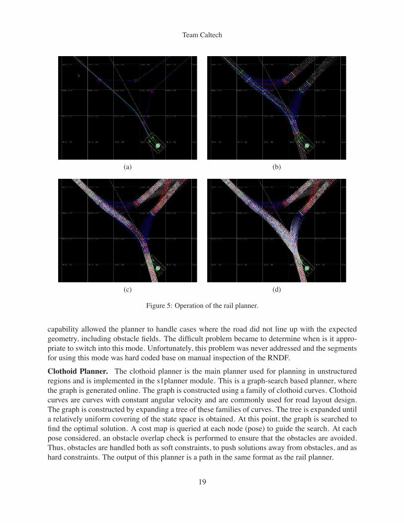
Rail Planner. The rail planner’s main function is to search over the precomputed graph to find theoptimal path to the goal. Since this graph is defined in the world frame, the planner has to plan inthe frame. The first step is to preprocess the map data. This data must be converted to either fieldsassociated with the nodes of the graphs or weights associated with edges. Thus, the precomputedgraph node locations are calculated and fixed offline, but the graph is updated online to reflectthe latest sensing information. Once this step is completed, the optimal path to the goal can becalculated. To accomplish this, the planner uses an A* algorithm to search the graph. The costfunction used in the optimization penalizes curvature, which is useful to avoid sharp maneuvers athigh speed. Furthermore, the cost function tends to keep the vehicle in the center of the perceivedlane. In addition, the obstacles are included in the cost generate plans that stay further away fromobstacles when possible. In this way the uncertainty associated with the sensed objects is accountedfor.

Figure 5 shows the different graphs created by the Rail Planner. The RNDF is first used to inferthe geometry of the road and a single rail is placed down the (inferred) center of the lane (a). Turnsthrough intersections are also defined. This is called the road graph. Since the road geometry isonly approximately known, more rails are added to each lane to make the set of solutions to besearched less restrictive (b). Rail changes and lane changes are then defined on what is now theplanning graph (c).

It was found that in some cases the precomputed graph was too constraining. This was becausethe rail change, lane changes and turns where precomputed. However, it was quite possible to haveto deal with an obstacle between these predefined maneuvers. A function was implemented inthis case to locally generate maneuvers (paths), called the vehicle-subgraph, that generated plansfrom the current location and connected to the precomputed graph as quickly as possible. This isshown in Figure 5d. This normally gives the planner enough flexibility to navigate these cases. Theplanning algorithm is also able to plan in reverse, when allowed, making the planner very capable.

As mentioned before, one of the concerns with using this planner is the inference of the roadgeometry from the RNDF. A mode of the planner was implemented where a local graph is gener-ated online. This graph is much more elaborate that the vehicle subgraph discussed above and this

18

Team Caltech

(a) (b)

(c) (d)

Figure 5: Operation of the rail planner.

capability allowed the planner to handle cases where the road did not line up with the expectedgeometry, including obstacle fields. The difficult problem became to determine when is it appro-priate to switch into this mode. Unfortunately, this problem was never addressed and the segmentsfor using this mode was hard coded base on manual inspection of the RNDF.

Clothoid Planner. The clothoid planner is the main planner used for planning in unstructuredregions and is implemented in the s1planner module. This is a graph-search based planner, wherethe graph is generated online. The graph is constructed using a family of clothoid curves. Clothoidcurves are curves with constant angular velocity and are commonly used for road layout design.The graph is constructed by expanding a tree of these families of curves. The tree is expanded untila relatively uniform covering of the state space is obtained. At this point, the graph is searched tofind the optimal solution. A cost map is queried at each node (pose) to guide the search. At eachpose considered, an obstacle overlap check is performed to ensure that the obstacles are avoided.Thus, obstacles are handled both as soft constraints, to push solutions away from obstacles, and ashard constraints. The output of this planner is a path in the same format as the rail planner.

19

Team Caltech

Velocity Planner. The velocity planner accepts a spatial path and time parameterizes this path toobtain a trajectory. The velocity planner takes into account path features such as stop lines, obsta-cles on the path and obstacles close to the path. The planner considers the path, which has all theinformation necessary for velocity planning encoded in it, and specifies a desired velocity profile.For example, it will bring Alice to a stop at a desired deceleration and at a desired distance awayfrom an obstacle. For obstacles on the side of the path, it will slow Alice down when passing closeto these obstacles. Lastly, the velocity planner considers the curvature of the path and adjusts thevelocities along the path accordingly. The velocity planner is compatible with the rail-, clothoid-and circle-planners. The output of the planner is a trajectory.

Prediction. Planning in an environment where the agents move at high speed requires some formof prediction of the future states of the mobile objects. Prediction of cars driving in urban environ-ments is eased by the structure imposed on the environment, but is complicated by noisy sensorydata and partial knowledge of the world state. The world state (map) and the mobile object’s po-sition in this world are necessary to determine behavior. Two approaches for prediction whereinvestigated: (1) prediction based on particle filters and (2) prediction utilizing the structure in theenvironment and simple assumptions on the velocities of the mobile agents. The former approachwas dropped since the data representation was not easily incorporated into the current planningapproach. The latter approach has the disadvantage of not being of much use in unstructuredregions.

The prediction information is used in two ways: first, the data is used to define restricted regionsaround mobile agents. This is especially useful when planning in intersections (such as merging)or planning lane changes. The second use is for dynamic conflict analysis. Here, the predictedfuture states of the mobile objects are compared to the planned trajectory of Alice. If a collisionis predicted, an obstacle is placed in the map that alters Alice’s plan and thus avoids a potentialcollision. Noisy measurements of the mobile object’s state can cause prediction to sometimes bevery conservative (when the velocity is off) or simply wrong (when the obstacle position in thepartially known road network is estimated wrong).

4.3 Low-level Control and Vehicle InterfaceThe lower-level functions of the navigation system were accomplished by a set of tightly linkedmodules that controlled the motion of the vehicle along the desired path and broadcast the currentstate of the vehicle to other modules.

Follower. The follower module receives a trajectory data structure from planner and state infor-mation from astate. It sends actuation commands to gcdrive. Follower uses decoupled longitudinaland lateral PID controllers, to keep Alice on the trajectory. The lateral controller uses a nonlinearcontroller that accounts for limits on the steering rate and angle, and modifies its gains based onthe speed of the vehicle [4].

Gcdrive. Gcdrive is the overall driving software for Alice. It works by receiving directives fromfollower over the network, checking the directives to determine if they can be executed and, ifso, sending the appropriate commands to the actuators. Gcdrive also performs checking on the

20

Team Caltech

state of the actuators, resets the actuators that fail, implements the estop functionality for Aliceand broadcasts the actuator state. Also included in the role of gcdrive was the implemention ofphysical protections for the hardware to prevent the vehicle from hurting itself. This includesthree functions: limiting the steering rate at low speeds, preventing shifting from occurring whilethe vehicle is moving, transitioning to the paused state in which the brakes are depressed andcommands to any actuator except steering are rejected. (Steering commands are still accepted sothat obstacle avoidance is still possible while being paused) when any of the critical actuators suchas steering and brake fail.

Astate. The astate module was responsible for broadcasting the vehicle position (position, orien-tation, rates) data. This module read data from the Applanix hardware and processed the data toaccount for state jumps. It then broadcast the world and local frame coordinate for the vehicle.

Reactive Obstacle Avoidance. To ensure safe operation, it was decided to implement a low-levelreactive obstacle avoidance (ROA) mechanism. This mechanism is the reason why the low-levelplanner needed to plan in the local frame. The ROA would evaluate LADAR data directly andwhen an object is detected within some box around Alice (which is velocity dependent), it wouldadjust the reference velocity of the trajectory to bring Alice to a stop in front of this object. Oneof the key issues that needed to be faced was making this mechanism sensitive enough to preventcollisions, but not so sensitive that it reacts to every false positive detection. Furthermore, the restof the planner stack needed to be told that ROA is active (otherwise Alice stops for no apparentreason). Lastly, their needed to be a mechanism to override the ROA, otherwise there are situationswhere Alice would just be stuck indefinitely.

5 Mission and Contingency ManagementDue to the complexity of the system and a wide range of environments in which the system must beable to operate, an unpredictable performance degradation of the system can quickly cause criticalsystem failure. In a distributed system such as Alice, performance degradation of the system mayresult from changes in the environment, hardware and software failures, inconsistency in the statesof different software modules, and faulty behaviors of a software module. To ensure vehicle safetyand mission success, there is a need for the system to be able to properly detect and respond tounexpected events related to vehicle’s operational capabilities.

Mission and contingency management is often achieved using a centralized approach where acentral module communicates with nearly every software module in the system and directs eachmodule sequentially through its various modes in order to recover from failures. As a result, thiscentral module has so much functionality and responsibility and easily becomes unmanageable anderror prone as the system gets more complicated. In fact, our failure in the 2005 Grand Challengewas mainly due to an inability of this central module to reason and respond properly to certaincombination of faults in the system. This results from the difficulty in verifying this module due toits complexity.

The contingency management subsystem comprises the mission planner, the health monitorand the process control modules. The Canonical Software Architecture (CSA) was developed to

21

Team Caltech

allow mission and contingency management to be achieved in a distributed manner. This functionworks in conjunction with the planning subsystem to dynamically replan in reaction to contin-gencies. The health monitor module actively monitors the health of the hardware and software todynamically assess the vehicle’s operational capabilities throughout the course of mission. It com-municates directly with the mission planner module which replans the mission goals based on thecurrent vehicle’s capabilities. The process control module ensures that all the software modulesrun properly by listening to the heartbeat messages from all the modules. A heartbeat messageincludes the health status of the software. The process control restarts a software module thatquits unexpectedly and a software module that identifies itself as unhealthy. The CSA ensures theconsistency of the states of all the software modules in the planning subsystem. System faults areidentified and replanning strategies are performed distributedly in the planning subsystem throughthe CSA. Together these mechanisms make the system capable of exhibiting a fail-ops/fail-safeand intelligent responses to a number different types of failures in the system.

5.1 Canonical Software ArchitectureThe modules that make up the planning system are responsible for reasoning at different levels ofabstraction. Hence the planning system is decomposed into a hierarchical framework. To supportthis decomposition and separation of functionality while maintaining communication and contin-gency management, we implemented the planning subsystem in a canonical software architecture(CSA) as shown in Figure 6. This architecture builds on the state analysis framework developed atJPL [2] and takes the approach of clearly delineating state estimation and control determination.To prevent the modules from getting out of sync because of the inconsistency in state knowledge,we require that there is only one source of state knowledge although it may be captured in differentabstractions for different modules.

A control module receives inputs and delivers outputs. The inputs consist of sensory reports(about the system state), status reports (about the status of other modules), directives/instructions(from other modules wishing to control this module), sensory requests (from other modules wish-ing to know about this modules estimate of the system state) and status requests (from other mod-ules wishing to know about this module status). The outputs are the same type as the inputs, but inthe reverse direction (reports of the system state from this module, status reports from this module,directives/instructions to other modules, etc).

For modularity, each module in the planning subsystem may be broken down into multipleCSA modules. A CSA module consists of three components—Arbitration, Control and Tactics—and communicates with its neighbors through directive and response messages, as shown in Figure7. Arbitration is responsible for (1) managing the overall behavior of the module by issuing amerged directive, computed from all the received directives, to the Control; and (2) reportingfailure, rejection, acceptance and completeness of a received directive to the Control of the issuingmodule. Control is responsible for (1) computing the output directives to the controlled module(s)based on the merged directive, received response and state information; and (2) reporting failureand completeness of a merged directive to the Arbitration. Tactics provides the core functionalityof the module and is responsible for generating a control tactic or a contiguous series of controltactics, as requested by the Control.

22

Team Caltech

Sensing andMapping

Subsystem

HealthMonitor

Applanix(GPS and

IMU)astate

Follower

Segment-level goals

Trajectory

Actuatorcommand

Actuatorcommand(includingresetcommand)

Connect/disconnectcommand

Vehicle capability

Actuator health

Vehicle stateestimation

health

Connect/disconnectcommand Sensor

health

World map

Local map

MDF

RNDF

Vehiclestate

Vehicle state

Mission Planner

Directive/response

State knowledge

Actuators

Sensors

Response

Response

Planner

Response

Response

Gcdrive

Response

Response

Figure 6: The planning subsystem in the Canonical Software Architecture. Boxes with double lined bordersare subsystems that will be broken up into multiple CSA modules.

5.2 Health Monitor and Vehicle CapabilitiesThe health monitor module is an estimation module that continuously gathers the health of thesoftware and the hardware of the vehicle (GPS, sensors and actuators) and abstracts the multitudesof information about these devices into a form usable for the mission planner. This form canmost easily be thought of as vehicle capability. For example, we may start the race with perfectfunctionality, but somewhere along the line lose a right front LADAR. The intelligent choice inthis situation would be to try to limit the number of left and straight turns we do at intersectionsand slow down the vehicle. Another example arises if the vehicle becomes unable to shift intoreverse. In this case we would not like to purposely plan paths that require a U-turn.

From the health of the sensors and sensing modules, the health monitor estimates the sensingcoverage. The information about sensing coverage and the health of the GPS unit and actuatorsallow the health monitor to determine the following vehicle capabilities: (1) turning right at in-tersection; (2) turning left at intersection; (3) going straight at intersection; (4) nominal drivingforward; (5) stopping the vehicle; (6) making a U-turn that involves reverse; (7) zone region oper-ation; and (8) navigation in new areas.

23

Team Caltech

Arbitration

Control Tactics

Merged directive: start/end conditions,parameterized constraints,performance criteria

Response:completed/

failed

InitializeA generic

control module

Directive: start/end conditions,parameterized constraints,performance criteria, priority

Response:accepted/rejected,

completed/failed

State informationDirective, state

Tactic

Controlling moduleSame interface withother controlling modules

Controlled module and/or Estimator or Hardware

DirectivesResponse

Figure 7: A generic control module in the Canonical Software Architecture.

5.3 Mission PlannerThe mission planner module receives the vehicle capabilities from the health monitor module, theposition of obstacles with respect to the RNDF from the mapper module and the MDF and sendsthe segment-level goals to the planner module. It has three main responsibilities and is broken upinto one estimation and two CSA control modules.

Traversibility Graph Estimator. The traversibility graph estimator module estimates the traversibil-ity graph which represents the connectivity of the route network. The traversibility graph is deter-mined based on the vehicle capabilities and the position of the obstacles with respect to the RNDF.For example, if the capability for making a left or straight turn decreases due to the failure of theright front LADAR, the cost of the edges in the graph corresponding to making a left or straightturn will increase, and the route involving the less number of these maneuvers will be preferred.If the vehicle is not able to shift into reverse, the cost of the edges in the graph corresponding tomaking a U-turn will be removed.

Mission Control. The mission control module computes the mission goals that specify how Alicewill satisfy the mission specified in the MDF and conditions under which we can safely continuethe race. It also detects the lack of forward progress and replans the mission goals accordingly.The mission goals are computed based on the vehicle capabilities, the MDF, and the responsefrom the route planner module. For example, if the nominal driving forward capability decreases,the mission control will decrease the allowable maximum speed which is specified in the mission

24

Team Caltech

goals, and if this capability falls below certain value due to the failure in any critical componentsuch as the GPS unit, the brake actuator or the steering actuator, the mission control will send apause directive down the planning stack, causing the vehicle to stop.

Route Planner. The route planner module receives the mission goals from the mission controlmodule and the traversibility graph from the traversibility graph estimator module. It determinesthe segment-level goals which include the initial and final conditions which specify the RNDFsegment/zone Alice has to navigate and the constraints, represented by the type of segment (road,zone, off-road, intersection, U-turn, pause, backup, end of mission) which basically defines aset of traffic rules to be imposed during the execution of this segment-level goals, in order tosatisfy the mission goals. The segment-level goals are transmitted to the planner module using thecommon CSA interface protocols. Thus, the route planner will be notified by the planner when asegment-level goal directive is rejected, accepted, completed or failed. For example, since one ofthe rules specified in a segment-level goal directive is to avoid obstacles, when a road is blocked,the directive will fail. Since the default behavior of the planner is to keep the vehicle in pause, thevehicle will stay in pause while the route planner replans the route. When the failure of a segment-level goal directive is received, the route planner will request an updated traversibility graph fromthe traversibility graph estimator module. Since this graph is built from the same map used by theplanner, the obstacle that blocks the road will also show up in the traversibility graph, resulting inthe removal of all the edges corresponding to going forward, leaving only the U-turn edges fromthe current position node. Thus, the new segment-level goal directive computed by the Control ofthe route planner will be making a U-turn and following all the U-turn rules. This directive willgo down the planning hierarchy and get refined to the point where the corresponding actuators arecommanded to make a legal U-turn.

5.4 Fault Handling in the Planning SubsystemIn our distributed mission and contingency management framework, fault handling is embed-ded into all the modules and their communication interfaces in the planning subsystem hierarchythrough the CSA. Each module has a set of different control strategies which allow it to identifyand resolve faults in its domain and certain types of failures propagated from below. If all thepossible strategies fail, the failure will be propagated up the hierarchy along with the associatedreason. The next module in the hierarchy will then attempt to resolve the failure. This approachallows each module to be isolated so it can be tested and verified much more fully for robustness.

Planner. The logic planner is the component that is responsible for fault handling inside theplanner. Based on the error from the path planner, the velocity planner and the follower, the logicplanner either tells the path planner to replan or reset, or specifies a different planning problem(or strategy) such as allowing passing or reversing, using the off-road path planner, or reducingthe allowable minimum distance from obstacles. The logic for dealing with these failures can bedescribed by a two-level finite state machine. First, the high-level state (road region, zone region,off-road, intersection, U-turn, failed and paused) is determined based on the directive from themission planner and the current position with respect to the RNDF. The high-level state indicatesthe path planner (rail planner, clothoid planner, or off-road rail planner) to be used. Each of the

25

Team Caltech

OFF-ROADmode

DR,NP,S STO,NP,Sno collision-free path exists Alice has been stopped for long

enough and there is an obstaclein the vicinity of Alice

passing finished or obstacle disappeared

DR,P,S STO,P,Sno collision-free path exists

collision-free path is foundno collision-free path existsand the number of times Alicehas switched to the DR,P,Rstate near the current positionis less than some threshold

DR,PR,S

no collision-free path exists and thenumber of times Alice has switchedto the DR,P,R state near the currentposition is less than some threshold

collision-free path is foundSTO,PR,S

BACKUP

no collision-freepath exists andthere is morethan one lane

no collision-freepath exists andthere is onlyone lane

backup finishedor failed and thenumber of times Alicehas switched to BACKUPis less than some threshold

DR,P,SSTO,P,Sno collision-free path exists

collision-free path is foundcollision-free path is found

no collision-freepath exists

no collision-free path exists and the number of times Alice has switched to the DR,P,Rstate near the current position exceeds somethreshold and there is more than one lane

no collision-free path exists and the number of times Alice has switched to the DR,P,Rstate near the current position exceeds some threshold and there is only one lane

STO,A

backup finished or failed and thenumber of times Alice has switchedto BACKUP exceeds some threshold

DR,Ano collision-free path exists

no collision-free path exists

collision-free path is found

collision-free path is found

collision-free pathwith DR,A is found

DR,B STO,Bno collision-free path exists

collision-free path is found

no collision-free path existsand there is more than one lane

collision-free path with DR,P,R is found

no collision-free path existsand there is only one lane

passing finished or obstacle disappeared

FAILED PAUSED

ROAD REGION

Figure 8: The logic planner finite state machine for the road region. Each state defines the drive state (DR #

drive, BACKUP, and STO # stop when Alice is at the right distance from the closest obstacle as specifiedby the associated minimum allowable distance from obstacles), the allowable maneuvers (NP # no passingor reversing allowed, P # passing allowed but reversing not allowed, PR # both passing and reversingallowed), and the minimum allowable distance from obstacles (S # safety, A # aggressive, and B # bare).

high-level states can be further extended to the second-level state which completely specifies theplanning problem described by the drive state, the allowable maneuvers, and the allowable distancefrom obstacles.

• Road region The logic planner transitions to the road region state when the type of segmentspecified by the mission planner is road. In this state, the rail planner is is the default pathplanner although the clothoid planner may be used if all the strategies involving using therail planner fail. There are thirteen states and twenty seven transitions within the road regionstate as shown in Figure 8. The DR,NP state is considered to be the nominal state. The logicplanner only transitions to other states due to obstacles blocking the desired lane or errorsfrom the other planners.

26

Team Caltech

SAFETY AGGRESSIVE

BARE

no collision-free path exists

timeout

no collision-freepath exists

FAILED

timeout

no collision-freepath exists

PAUSED

ZONE REGION

DR,S STO,Sno collision-free path exists

collision-free pathwith DR,S is found

DR,A STO,A

no collision-freepath exists

no collision-free path exists

collision-free path is found

collision-free path is foundno collision-freepath exists

STO,BDR,Bno collision-free path exists

collision-free path is found

collision-free pathwith DR,A is found

FAILED

no collision-freepath exists

PAUSED

OFF-ROAD

(a) (b)

Figure 9: The logic planner finite state machine for the zone region (a) and off-road (b). Each state definesthe drive state (DR # drive, and STO # stop when Alice is at the right distance from the closest obstacleas specified by the associated minimum allowable distance from obstacles) and the minimum allowabledistance from obstacles (S # safety, A # aggressive, and B # bare).

• Zone region The logic planner transitions to the zone region state when the type of segmentspecified by the mission planner is zone. Reversing is allowed and since the clothoid planneris the default path planner for this state, the trajectory is planned such that Alice will stop atthe right distance from the obstacle by default, so only three states and four transitions arenecessary within the zone region state as shown in Figure 9(a).

• Off-road The logic planner transitions to the off-road state when the type of segment speci-fied by the mission planner is off-road. Since passing and reversing are allowed by default,six states and ten transitions are necessary within the off-road state as shown in Figure 9(b).

• Intersection The logic planner transitions to the intersection state when Alice approaches anintersection. In this state, passing and reversing maneuvers are not allowed and the trajectoryis planned such that Alice stops at the stop line. The rail planner is the default path planner.Once Alice is within a certain distance from the stop line and is stopped, the intersectionhandler, a finite state machine comprising five states (reset, waiting for precedence, waitingfor merging, waiting for the intersection to clear, jammed intersection, and go), will be resetand start checking for precedence. The logic planner will transition out of the intersectionstate if Alice is too far from the stop line, when Alice has been stopped in this state fortoo long, or when the intersection handler transitions to the go or jammed intersection state.If the intersection is jammed, the logic planner will transition to the state where passing isallowed.

• U-turn The logic planner transitions to the U-turn state when the type of segment specifiedby the mission planner is U-turn. In this state, the default path planner is the clothoid planner.Once the U-turn is completed, the logic planner will transition to the paused state and wait

27

Team Caltech

for the next command from the mission planner. If Alice fails to execute the U-turn due toan obstacle or a hardware failure, the logic planner will transition to the failed state and waitfor the mission planner to replan.

• Failed The logic planner transitions to the failed state when all the strategies in the currenthigh-level state have been tried. In this state, failure is reported to the mission planner alongwith the associated reason. The logic planner then resets itself and transitions to the pausedstate. The mission planner will then replan and send a new directive such as making a U-turn, switching to the off-road mode, or backing up in order to allow the route planner tochange the route. As a result, the logic planner will transition to a different high-level state.These mechanisms ensure that Alice will keep moving as long as it is safe to do so.

• Paused The logic planner transitions to the paused state when it does not have any segment-level goals from the mission planner or when the type of segment specified by the missionplanner is pause or end of mission. In this state, the logic planner is reset and the trajectoryis planned such that Alice comes to a complete stop as soon as possible.

Follower. Although a reference trajectory computed by the planner is guaranteed to be collision-free, since Alice cannot track the trajectory perfectly, it may get too close or even collide with anobstacle if the tracking error is too large. To address this issue, we allow follower to request a replanfrom the planner through the CSA directive/response mechanism when the deviation from thereference trajectory is too large. In addition, we have implemented the reactive obstacle avoidance(ROA) component to deal with unexpected or pop-up obstacles. The ROA component takes theinformation directly from the perceptors (which can be noisy but faster) and can override theacceleration command if the projected position of Alice collides with an obstacle. The projectiondistance depends on the velocity of Alice. The follower will report failure to the planner if theROA is triggered, in which case the logic planner can replan the trajectory or temporarily disablethe ROA. We have also formally verified that through the use of the CSA, follower either has theright knowledge about the gear Alice is currently in even though it does not talk to the actuatordirectly and the sensor may fail; otherwise, it will send a full brake command to the gcdrive.

6 ResultsExtensive testing on Alice was used to validate its capabilities and tune its performance. Thissection summarizes the major results of this testing.

6.1 Site VisitThe site visit consisted of four separate runs around a simple course consisting of a single inter-section and a circular loop, as shown in Figure 10. After initial safety inspection and e-stop test,the first run consisted of driving around the loop once and was performed successfully.

The second run was a path planning run, in which a set of sparse waypoints were given anda route had to be planned that included performing U-turn operations in the stubs. On our first

28

Team Caltech

Figure 10: Site visit course.

attempt at this run, the vehicle failed to perform the U-turn successfully, with an apparent loss ofsteering. A combination of high temperatures and a road surface that created large frictional forceswith the tires caused a torque limit to be reached in the motor controller, resulting in a reset inthe steering controller. This problem was remedied in a second attempt (after the fourth run) byreseting an internal parameters that lowered the commanded steering at slow speeds. After thischange the test was performed successfully.

The third run involved driving multiple times around the loop with obstacles (stationary cars)placed at various points on the route. Alice detected and avoided all obstacles, and completed therun. For tests in which a vehicle was in the lane of travel, Alice signaled properly to move out ofthe lane and transitioned out of the lane at the required distances. Alice did not transition backinto the lanes within the required distances, an artifact of the way in which the planning algorithmwas implemented (there was an insufficiently high cost associated with gradually returning to theproper lane).

The fourth run focused on intersection operations. The run consisted of driving multiple timesaround the loop, with cars positioned at the intersection in different situations for each loop. Aliceproperly detected vehicles and respected the precedence order except for two occasion.

• In one instance, there were two cars queued up at the intersection opposite Alice. WhenAlice approached the intersection, it stopped, waiting a few seconds, and then continuedthrough the intersection. According to the safety driver (who was in Alice), we had a smallreturn coming up to the intersection and then the LADARs tilted down when we stopped.This caused the obstacles to disappear completely (the map subsystem had no memory at thispoint) and then reappear, so Alice decided that we were the first vehicle at the intersection.

• In the second instance, two vehicles were queued to the left of Alice. We stopped at theintersection and waited for the first vehicle. After that vehicle passed, we continued to waitat the intersection. After waiting for a while, DARPA motioned the second vehicle to gothrough and at that point Alice properly continued through the intersection. According to the

29

Team Caltech

Figure 11: St. Luke Medical Center (Pasadena, CA)

internal logs, the second vehicle was partially in the opposing lane and that Alice interpretedthis as a vehicle in the intersection, so it remained stopped.

While the site visit was executed more or less successfully, we identified several of limitationsin the design. A major difficulty in preparing for the site visit was the brittleness of the finite statemachine logic that accounted for traffic rules. Even with the limited complexity of the site visittasks, the planner had dozens of states to account for different environmental conditions and drivingmodes. This made the planner very hard to debug. Some of the lower level control functions(including path following) were also found to be lower performance that we desired for the race.And finally, the accuracy and persistence of the sensed data need to be improvied.

The primary changes that were made after the site visit were (1) to simplify the traffic logicto use a very small number of modes; (2) to redesign the planning subsystem so that it madeuse of a graph-based planner instead of the originally proposed NURBS-based planner and (3)to streamline the planner software structure so that it acted as a single CSA module rather thanseparate modules for each internal function. These changes coincided with a decision to separatethe path planning problem into a spatial planner (rail-planner) and a temporal planner (velocity-planner), rather than the originally planned spatio-temporal planner (dplanner). In addition, werewrote the low-level control algorithms (follower) and implemented more robust functionality fordetecting and tracking objects.

6.2 Summer TestingDuring the summer of 2007, extensive testing and development was performed at two primary testsites: the former St. Luke Medical Center in Pasadena, CA and El Toro Marine Corps Air Stationin Irvine, CA. Over the course of three months, approximately 300 miles of fully autonomousdriving was performed in these locations.

Testing at the St. Luke Medical Center was performed in the (empty) parking lot of the facility,shown in Figure 11. While this area was quite small for testing, its proximity to Caltech allowed

30

Team Caltech

Figure 12: El Toro Marine Core Air Station test area (Irvine, CA).

us to use the facility frequently and easily. A standard course was set up which could be used toverify the basic driving functionality and track performance. Some of the features of this courseincluded tight turns, sparse waypoint areas, parking zones, overhanging buildings and trees, andtight maneuvering between structures.

El Toro Marine Corps Air Station was used for more extensive testing. This base is no longerin active use and was available for lease through a property management corporation. The primaryRNDF used for testing is shown in Figure 12 This facility had all of the features specified in theDARPA Technical Criteria, including multiple types of intersections, multi-lane roads, parkingzones, off-road sections, sparse waypoints, overhanging trees and tightly spaced buildings.

A total of 15 days of testing at El Toro were used to help tune the performance of the vehicle.The first long run with no manual interventions was a run of 11 miles on 19 September 2007,approximately 6 weeks before the race. The most number of miles driven in a single day was40.5 miles on 16 October 2007. The highest average speed on a run of over 5 miles was 9.7miles/hour on 16 October 2007. Additional testing included intersection testing with up to fivevehicles, merging across traffic with cars coming from both directions, and defensive driving withtraffic coming into the lane from a driveway and oncoming traffic driving in the incorrect lane.

6.3 National Qualifying EventIn this section we describe Team Caltech’s performance in each of the three NQE test areas. Wepresent each run in chronological order.

Run 1: Area B, Attempt 1. Area B consisted of tasks in basic navigation, including routeplanning, staying in lanes, parking and obstacle avoidance. An overview of Area B is shown inFigure 13. Basic navigation, stay in lane, parking. The MDF started in the starting chute area, thendirected Alice to proceed down a road onto the main course. From there, the MDF direted Alice todrive down several different roads on the interiod of the course and eventually return to the startingarea.

31

Team Caltech

Figure 13: Test Area B

Alice encountered several difficulties on this run. First, the K-rails (concrete traffic barriers)in the startup chute were less than 1m away from Alice and the vehicle did not want to leavethe chutes immediately. The same problem occurred at the exit of the startup area where K-railsformed a narrow gate. In order to proceed through the area, Alice had to progress through a seriesof internal planning failures before finally driving with reduced buffers on each side of the vehicle.After successfully leaving the area after about 5 minutes, Alice was performing well on the roadsand entered the parking zone in the south part of the course. The spacing of the vehicles to eachside of Alice was less than the required 1 meter buffer and Alice spent substantial time attemptingto reorient itself to park in the spot. Once in the spot, Alice was unable to pull fully into theparking spot because the car in front of it was closer than the required 2 meter buffer. Alice wasthen manually repositioned and continued its run for a short period before the 30 minute time limitwas reached.

As a result of this run, the code was changed to allow passing obstacles that are closer than1m away from the vehicle. In addition, the tolerance of reaching waypoints in parking zones wasrelaxed.

Run 2: Area A: Attempt 1. This test consisted of merging into traffic with 10–12 mannedvehicles circling around a “block”, as shown in Figure 14. Vehicles are started in the center laneof the course and are supposed to make constant left turns, proceeding around the left loop ofthe course in the counterclockwise direction. Four vehicles with approximately equal spacing arecircling around the larger loop in the counterclockwise direction. Six or more vehicles clusteredtogether in groups of 1, 2 or 3 vehicles are circling the opposite direction. At the south intersection,Alice needs to merge into traffic after crossing one lane. At the north intersection Alice is supposedto make a left turn into oncoming traffic. The manned vehicles had a separation distance of 2 to 20seconds. Therefore Alice had to sense a 10 second or longer gap and merge quickly into the gap.

In the first attempt of NQE run A, several bugs were uncovered. The first occured when Aliceentered the intersection after determining that the path was clear. The proximity of a set of concretebarriers to the road meant that Alice could not complete the turn without coming close the the

32

Team Caltech

Figure 14: Test Area A

barriers. The low-level reactive obstacle avoidance logic was using a different threshold for safeoperation on the side of the vehicle (2 meters instead of 1 meter) and hence it would stop the vehiclepartway through the intersection. This caused the intesection to become jammed (and generatedlots of honks).

A second, related bug occurred in the logic planner that affected our wait at the intersectionproperly. While the intersection handler was active, another part of the higher-level logic plannercould switch into the STOPOBS state if it detected a nearby vehicle (e.g, one of the human-drivencars was predicted to collide with Alice or its buffer region). This change in state de-activated theintersection handler and could cause the vehicle to enter the intersection when the path becameclear (without invoking the proper merge logic). Table 1 gives a detailed analysis of the operationat each intersection. While in some cases the intersection handler was just interrupted but calledagain, it was canceled completely in other cases. If it was canceled, prediction was also not active.In these cases it almost caused two accidents with manned vehicles. At the north intersection, thesoftware bug did not occur as logic planner did not switch into STOPOBS. This can be explainedby the fact that by the nature of this intersection, no vehicle was crossing in front of Alice. As aresult, merging was clean in all 7 scenarios at the north intersection.

Fixing the issues that were uncovered during this test required extensive changes at the NQE.First, the logic for reactive obstacle avoidance had to be changed to use a different safety bufferlength in the front of the vehicle versus the sides (consistent with the logic used by the planner).Secondly, a rather major restructuring of the logic planner was required to insure that it did notskip the intersection handling logic until it had actually cleared an intersection. The changes weredifficult to test at the NQE, even with extensive use of the testing areas (where no live traffic wasallowed) and simulation.

Run 3: Area C, Attempt 1. Area C was designed to test intersection precedence, route planningand U-turn capabilities. The RNDF consisted of two intersections connected by a set of three roads,as shown in Figure 15. The major task in NQE run C was the correct handling of intersections withvehicles having precedence and to perform a U-turn at a road block. At the start of the run, the

33

Team Caltech

Table 1: Analysis of performance in Area A, Attempt 1.Location Vehicles Missed Time Comments

passed gaps passed#1 S 8 N/A 32.0s Interrupted by STOPOBS; prediction active#2 N 1 0 7.7s Clean merge#3 S 6 N/A 17.0s Interrupted by STOPOBS; prediction active#4 N 2 0 14.6s Clean merge#5 S 11 1 >60.0s Canceled by STOPOBS; prediction not active.

Almost hit vehicle#6 N 0 0 21.0s Stopped too far left; other vehicles stopped#7 S 3 N/A 23.0s Canceled by STOPOBS; prediction not active#8 N 3 0 16.3s Clean merge#9 S 6 0 38.2s Clean merge

#10 N 1 0 7.9s Clean merge#11 S 4 N/A 12.0s Canceled by STOPOBS; prediction not acti-

vated. Almost hit vehicle#12 N 0 0 9.4s Stopped too far left; other vehicles stopped#13 S 6 N/A 34.0s Interrupted by STOPOBS; clean merge#14 N 0 0 4.2s Clean merge

Figure 15: Test Area C

inner road between the intersection is blocked and the other roads are opened. The vehicle iscommanded to go in a loop between the two intersections. At each successive intersection, a morecomplicated scenario is established. On the final run, one of the outer paths is blocked, requiringthe vehicle to replan and choose a different route.

Table 2 gives an analysis of Alice’s performance. The columns of the table indicate the inter-section that was encountered, the number of vehicles at the intersection that had precedence at thetime Alice arrived, the number of vehicles detected by Alice, and the number of times visibilitywas occluded by another vehicle.

Alice gave precedence correctly at all 7 intersections. At intersection #2 it was by accident that

34

Team Caltech

Table 2: Analysis of performance in Area C, Attempt 1.Loc # Veh # Veh Lost Dur. Comments

w/ prec seen visibility#1 N 0 0 0 2.4s Empty intersection. Correct execution#2 S 1 1 N/A N/A Interrupted by steering fault. Correct execution#3 N 2 2 0 25.8s Correct execution

#4 S 2 2 1 25.8s Correct execution. One vehicle was blocking Al-ice’s view while passing through intersection

#5 N 3 3 1 34.8s Correct execution. One vehicle was blocking Al-ice’s view while passing through intersection

#6 S 1 1 2 25.8s Following at intersection, then giving precedence.Correct execution.

#7 N 3 3 2 37.8s Correct execution. One vehicle was blocking Al-ice’s view while passing through intersection

the power steering problems occurred when the other vehicle had already passed the intersection.While Alice was stationary, a troque fault in the steering caused a lower-level module to pauseAlice for safety reasons. This event also triggers planner to switch into the state PAUSE whichstops the intersection handling algorithm. After the system started up again and the intersectionhandler was called, the intersection was clear and Alice passed the intersection. Otherwise Alicemight have made wrong assumptions about the time of arrival of other vehicles. The results fromthis run also demonstrate that ID tracking, checking for lost IDs and checking for visibility arecrucial to the correct execution of the precedence. Without those backup algorithms, Alice wouldhave misinterpreted the precedence order at intersections or would have lost vehicles in its internalprecedence list.

After the intersection tests, Alice had to demonstrate correct execution of U-turns in frontof road blocks. A bug was introduced in implementing the changes from Area A that caused themission planner to crash during certain U-turn operations. The process controller properly restartedthe mission planner after the crash, but Alice lost information regarding which part of the road wasblocked. It thus alternated between the two road blocks and the run could not be finished withinthe time out limit but was considered a successful clean run.

The bug that caused the mission planner to crash was fixed in response to the results from thisrun.

Run 4: Area B, Attempt 2. Despite fixing the problems near the starting chute based on theprevious attempt in Area B, Alice still had difficulty initializing to the properly state when it wasplaced in the startup chute. Due to delays in the launch of the vehicle by DARPA, we were able tocorrect the logic in the chute and launch the vehicle correctly.

With the changes in the buffer region, Alice was able to traverse through the start area andonto the course with little difficulty. At one point toward the beginning of the run, the controlvehicle paused Alice because it appeared to be headed toward a barrier. This appears to be due toa checkpoint that was close to a barrier and hence Alice was coming close to the barrier in order tocross over the checkpoint. Alice was put back into run mode and continued properly.

The remainder of the run was completed with only minor errors. Alice properly parked in

35

Team Caltech

Table 3: Analysis of performance in Area A, Attempt 2.Time Action Failure Comments

#1 14:14:42 Merging, S inters’n Clean merging after 14.9 s

#2 14:15:05 Exit of inters’n Alice stopped Stopped because of close obsta-cles and prediction

#3 14:15:56 Left turn Problems following tightleft turn, hit curb Path/follower problems

#4 14:16:21 Merging, N inters’n Clean merging after 38.6s

#5 14:17:21 Stopping, S inters’n Stop line problemsDidn’t stop at stop line and droveinto intersection. Paused byDARPA

#6 14:19:21 Merging, N inters’n Clean merging after 20.1s

#7 14:20:01 Stopping, S inters’n Stop line problemsDidn’t stop at stop line and droveinto intersection. Paused byDARPA

#8 14:21:04 Exit out of inters’n Pulling into on cominglane

Prediction stopped Alice, butmanned car performed evasivemaneuver. Paused by DARPA

#9 14:22:28 End of run

the parking lot (the cars on the sides had been removed) and proceeded through the “gaunltet”, astretch of road in which a variety of obstacles had been placed. It then continued driving downseveral streets and through the northern zone, which had an opening in the fence. At several pointsin the run Alice ran over the curb after turning at intersections. Alice completed the mission inabout 23 minutes.

Run 5: Area A, Attempt 2. In the second attempt at Area A, Alice’s logic had been updatedto ensure that intersection handler would not be overwritten by changing into another state withinthe logic planner’s state machine. Unfortunately, an unrelated set of bugs caused problems onthe second attempt. Table 3 summarizes the major events on this run. The primary errors in thisrun consisted of properly detecting the stop lines, which appeared in the logs to jump around in amanner that had not been previously seen (either in testing or other NQE runs).

To understand what happened at the stop lines, a bit more detail is required. The followingsteps and conditions that are necessary to stop at stop lines:

• Path planner - Creates path to stay in lane and to follow turns• Planner - Search for stop lines close to path and store stop line information within the path

structure• Logic planner - Computes distance between Alice and next stop line found within path struc-

ture• Logic planner - Depending on distance to stop line, switch in state STOP INTERSECTION• Velocity planner - Detects state STOP INTERSECTION and modify velocity plan

These steps are necessary as the (spatial) path planner does not take into account stop lines, but

36

Team Caltech

instead relies on the velocity planner to bring the vehicle to a stop. Therefore the function to findthe closest stop line is the critical part of the algorithm.

All modules communicate with the skynet framework. During the race all skynet messageswere written into a log file. Therefore the complete run can be replayed. Watching this replayand checking the log files, it became obvious that the main problem happened in computing thedistance between Alice and the next stop line. To find the closest stop line, Alice performs thefollowing actions:

• Search for all RNDF stop lines within this rectangle• Project found RNDF stop lines onto path and choose closest• Query map to obtain sensed stop line position for this stop line• Choose closest node within path, required for velocity planner

In previous runs, sensed stop lines were only stored for 5 cycles after they were not picked upanymore by the sensors. This threshold was increased during the NQE as stop lines could not beseen by sensors when Alice’s body was hiding the stop lines. Having a longer time-to-live value,false-positives were stored longer in the map. At this time, wrong data association in the map leadto jumping stop lines. When the vehicle approached the stop line in lap #2 and lap #3 the dataassociation was right while approaching the intersection. As it came closer to the real stop line,the mapper bug assigned a false-positive stop line that was 3.2 meters behind Alice. In this case,Alice is assumed to have passed the stop line and did not stop as the threshold for passing a stopline was set to 3.0 meters. In lap #3 the stop line was moved ahead so that Alice was aiming fora stop line that was in the middle of the intersection. There was no algorithm in place detectingsudden changes in stop line positions.

7 Accomplishments and LessonsAlthough Alice di not qualify for the race in 2007, the development of an autonomous vehiclecapable of driving in urban traffic was very educational and rewarding. In this section we documentsome of the lessons learned and contributions of the project.

7.1 Lessons LearnedTeam Caltech’s approach to the Urban Challenge built on our experience from 2005, in which acombination of low-level failures were not properly handled by the software and Alice drove overa concrete barrier. To help mitigate the chances of a similar failure in 2007, a substantial effort wasplaced on systems engineering and systems architecture. Unfortunately, bugs that were similar innature to what we experienced in 2005 again caused critical failures (this time in the qualifyingevent). As in 2005, the failure occurred in a situation that was not well-reflected in our testing andpreparations.

The root cause for the fragilities in our system was lack of time and experience required todevelop the software required for the Urban Challenge. Our original schedule planned on having

37

Team Caltech

a fully functional system two months prior to the race, allowing ample time for testing and tuning.In reality, this point of technical progress was only reached approximately 2 weeks before the race,which meant that we were not able to test the software in a wide enough variety of situations touncover some of the bugs and performance issues.

At a high level, the software architecture that was developed appears to be capable of perform-ing autonomous operations at the level required for urban driving. With the exception of errors inrobustly detecting stop lines, the sensing subsystem performed well and was extremely capable.The planning subsystem was more brittle and the finite state machine used to control the overallfunctioning of the planner proved to be difficult to verify and modify.

7.2 Technical Contributions and Transitions

Technical Contributions. Through this contact, the following technical contributions have beenaccomplished:

New technologies for mission and contingency management - A directive/response based architec-ture was developed to provide the ability to reason about complex, uncertain, spatio-temporal en-vironments and to make decisions that enable autonomous missions to be accomplished safely andefficiently, with ample contingency planning. Building on expertise in high confidence decision-making and autonomous mission management at JPL, algorithms were developed to control thevehicle’s sensing, estimation, mapping, planning and control systems in complex and uncertainconditions, while also ensuring safe operations.

Distributed sensor fusion, mapping, and situational awareness - Building on Caltech and JPL expe-rience in sensory-based navigation—including feature classification and tracking, moving obstacledetection and tracking, visual odometry, and sensory-based mapping and localization—we devel-oped a multi-layer decomposition of our sensed environment so that different levels of navigationand contingency management algorithms could operate in parallel while providing highly robustand safe operation. These modules operated in a highly distributed computational architecture.

Real-time, optimization-based navigation - we developed an optimization-based approach to guid-ance, navigation and control (GNC) that allows our vehicle to plan and execute locally optimalpaths using a sensor-driven description of its environment. This approach was able to handle suchissues as moving vehicles, traffic laws and defensive driving.

Transitions. Through this activity, we have established a strong working relationship with theSpace Technologies sector of Northrop Grumman, including testing of advanced algorithms formotion planning on Alice (outside of the DGC program). We are also in discussions with the Sys-tems Integration sector of Northrop Grumman regarding their interest in developing autonomousvehicle technologies for airport operations.

In addition, Caltech is currently supported under a Multidisciplinary University Research Ini-tiative (MURI) grant in “Specification, Design and Verification of Distributed Embedded Systems”which will make use of our 2007 Urban Challenge experience (and our experimental platform) topursue research in formal verification methods for complex, autonomous systems such as Alice.

38

Team Caltech

Acknowledgments. The research in this paper was supported bin part by the Defense AdvancedResearch Projects Agency (DARPA) under contract HR0011-06-C-0146, the California Instituteof Technology, Big Dog Ventures, Northrop Grumman Corporation, Mohr Davidow Ventures andApplanix Inc.

The authors would also like to thank the following members of Team Caltech who contributedto the work described here: Daniel Alvarez, Mohamed Aly, Brandt Belson, Philipp Boettcher, JuliaBraman, William David Carrillo, Vanessa Carson, Arthur Chang, Edward Chen, Steve Chien, JayConrod, Iain Cranston, Lars Cremean, Stefano Di Cairano, Josh Doubleday, Tom Duong, LukeDurant, Josh Feingold, Matthew Feldman, Tony & Sandie Fender, Nicholas Fette, Ken Fisher,Melvin Flores, Brent Goldman, Jessica Gonzalez, Scott Goodfriend, Sven Gowal, Steven Gray,Rob Grogan, Jerry He, Phillip Ho, Mitch Ingham, Nikhil Jain, Michael Kaye, Aditya Khosla, Mag-nus Linderoth, Laura Lindzey, Ghyrn Loveness, Justin McAllister, Joe McDonnell, Mark Milam,Russell Newman, Noele Norris, Josh Oreman, Kenny Oslund, Robbie Paolini, Jimmy Paulos,Humberto Pereira, Rich Petras, Sam Pfister, Christopher Rasmussen, Bob Rasumussen, DominicRizzo, Miles Robinson, Henrik Sandberg, Chris Schantz, Jeremy Schwartz, Kristian Soltesz, ChessStetson, Sashko Stubailo, Tamas Szalay, Daniel Talancon, Daniele Tamino, Pete Trautman, DavidTrotz, Glenn Wagner, Yi Wang, Albert Wu, Francisco Zabala and Johnny Zhang.

References[1] L. B. Cremean, T. B. Foote, J. H. Gillula, G. H. Hines, D. Kogan, K. L. Kriechbaum, J. C.

Lamb, J. Leibs, L. Lindzey, C. E. Rasmussen, A. D. Stewart, J. W. Burdick, and R. M. Murray.Alice: An information-rich autonomous vehicle for high-speed desert navigation. Journal ofField Robotics, 23(9):777–810, 2006.

[2] D. Dvorak, R. D. Rasmussen, G. Reeves, and A. Sacks. Software architecture themes in jpl’smission data system. In Proceedings of 2000 IEEE Aerospace Conference, 2000.

[3] M. Ingham, R. Rasmussen, M. Bennett, and A. Moncada. Engineering complex embeddedsystems with state analysis and the mission data system. J. Aerospace Computing, Informationand Communication, 2, 2005.

[4] M. Linderoth, K. Soltesz, and R. M. Murray. Nonlinear lateral control strategy for nonholo-nomic vehicles. In Proc. American Control Conference, 2008. Submitted.

[5] C. Looman. Handling of dynamic obstacles in autonomous vehicles. Master’s thesis, Univer-sitat Stuttgart, 2007.

[6] H. Pereira. Road marking for an autonomous vehicle in dynamic environments. Technicalreport, Faculdade de Engenharia da Universidade do Porto, 2007.

[7] R. D. Rasmussen. Goal based fault tolerance for space systems using the mission data system.In Proceedings of the 2001 IEEE Aerospace Conference, 2001.

39

Team Caltech

A Additional Software ModulesIn addition to the software modules described in the main text, a number of other modules wereused as part of our system. Those modules are briefly described here.

ASim. Asim is a dynamic simulator for Alice that replaces the astate module. It accepts commentsfrom gcdrive, simuilates the dynamics of the vehicle (including wheel slippage), and broadcaststhe current vehicle state in a format compatible with astate.

Cotk. CoTK (Console Tool Kit) is a very basic display toolkit for text consoles. Implemented asa very thin layer over ncurses.

Circle Planner. The circle planner was one of two backup planners for the unstructured regions.This planner also constructed a graph from a family of curves. The curves considered in this casewas circular arcs and straight line segments. This was a feasibility planner, and did not incorporatecost from the cost map. It considered obstacles as hard constraints. The graph search was donewith an A* algorithm. This planner was very fast, and produced dynamically feasible solutions,but the solutions looked rather crude due to the family of curves used, which could easily havebeen remedied. This planner was tested but not used in the race.

DPlanner. An optimization-based planner was developed based on the use of NURBS basisfunctions combined with differential flatness, as described in the original proposal. This plannerrelied on a set of proprietary optimization algorithms that were developed by Northrop Grumman.The planner solves the complete spatio-temporal problem and is thus capable of accounting forthe dynamic obstacles in the environment explicitly. The planner operated on a cost map, but alsoenforced hard constraints for obstacles. The solution obtained (a trajectory) satisfies the dynamicsof the vehicle, as well as constraints on the inputs and state of Alice, while minimizing some costfunction. The NURBS-based planner was not able to execute quickly enough to run in real-time,and so a rail-based planner was developed to replace it. The dplanner module was not used in therace.

MapViewer. A lightweight 2-D map and map object viewer built using FLTK. Mapviewer can beused to visualize map elements sent in and out of the mapper module.

RNDF-editor. A JAVA GUI program for editing RNDF files.

Skynet. The skynet library is used for group communications in Alice. It is a fairly thin wrapperaround Spread. It supports broadcasting of messages to a given group name and subscribing togroups to receive relevant messages.

Sparrow. Sparrow is a collection of programs and a library of C functions intended to aid in theimplementation of real-time controllers on Linux-based data acquisition and control systems. Itcontains functions for executing control algorithms at a fixed rate, communicating with hardwareinterface cards, and displaying data in real-time. For the DGC, the real-time data display was theprimary usage.

40