Journal of Environmental Protection, 2015, 6, 837-850 Published Online August 2015 in SciRes. http://www.scirp.org/journal/jep http://dx.doi.org/10.4236/jep.2015.68076
How to cite this paper: da Silva, M.G., de Oliveira de Aguiar Netto, A., de Jesus Neves, R.J., do Vasco, A.N., Almeida, C. and Faccioli, G.G. (2015) Sensitivity Analysis and Calibration of Hydrological Modeling of the Watershed Northeast Brazil. Jour-nal of Environmental Protection, 6, 837-850. http://dx.doi.org/10.4236/jep.2015.68076
Sensitivity Analysis and Calibration of Hydrological Modeling of the Watershed Northeast Brazil Marinoé Gonzaga da Silva*, Antenor de Oliveira de Aguiar Netto, Ramiro Joaquim de Jesus Neves, Anderson Nascimento do Vasco, Carina Almeida, Gregório Guirado Faccioli Campus São Cristóvão, Federal Institute of Sergipe, São Cristóvão, Brazil Email: *[email protected] Received 1 June 2015; accepted 18 August 2015; published 21 August 2015
Abstract Mathematical models of the quantity and quality of water in hydrographic basins enable simula-tion of a wide variety of processes, including the production of water and sediments, and the dy-namics of point and nonpoint sources of pollution. These models have become increasingly com-plex, requiring large amounts of input data, which can increase the uncertainty of the results of simulations. For this reason, it is essential to perform calibration and validation procedures. The objective of this work was to conduct sensitivity analysis and calibration of a distributed hydro-logical model (SWAT) applied to the flows of water in the watershed of the Poxim River. Satisfac-tory performance of the model was indicated by the values obtained for the Nash-Sutcliffe effi-ciency coefficient (0.77), the percent bias (5.05), the root mean square error (0.48), and the ratio of the RMSE to the standard deviation of the observations (RSR) (0.49). The set of parameters identified here could be used for the simulation and evaluation of other scenarios.
1. Introduction The degradation of hydrological resources has made it essential to encourage management practices based on knowledge of spatial and temporal changes in the quantity and quality of water, in order to ensure the suitability of water supplied for different uses. This can be assisted by using hydrological and water quality models to si-
mulate a wide range of processes in hydrographic basins, such as the production of water and sediments and the dynamics of point and nonpoint sources of pollution.
Advances in computational capacity have meant that these models have become increasingly complex and require greater numbers of input parameters. This, in turn, can lead to increased uncertainties in the models. In principle, the parameters of a physically based model do not need to be calibrated, because the input data are obtained from field measurements. Nonetheless, the effects of spatial variability, measurement errors, incom-plete description of the elements and processes of a system, and the extrapolation of information for one point to locations for which measurements are not available, amongst other factors, mean that the values of many para-meters cannot be known with precision. Uncertainties may also be related to the model inputs, since for eco-nomic reasons the input data are often only measured at a limited number of locations. It is therefore necessary to calibrate models of hydrographic basins [1]-[4].
Using simulations, uncertainties in the management of a watershed can be reduced by evaluating different scenarios before they occur [5]. Water quality models employ a large quantity of parameters, resulting in a range of data sets that can be used to compare with the predictions of the model. Sensitivity analyses are then needed in order to accommodate the large number of parameters and multiple output variables [6].
The objective of this work was to perform a sensitivity analysis and calibration of flows in the watershed of the Poxim River, using the SWAT distributed hydrological model, in order to provide a tool for evaluation of management practices that could potentially help to reduce diffuse sources of pollution derived from agricultural practices in the hydrographic subbasins.
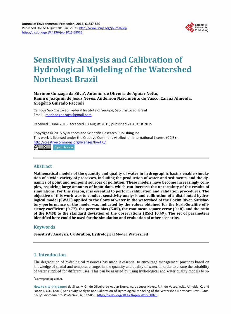
2. Materials and Methods 2.1. Study Region The study was performed in the watershed of the Poxim River, an area of 116.11 km2 that forms part of the wa-tershed of the Sergipe River (one of the most important rivers in Sergipe State). Located in the east of the State, the Sergipe River basin includes parts of the municipalities of Itaporangad’ Ajuda, AreiaBranca, Laranjeiras, NossaSenhora do Socorro, São Cristóvão, and Aracaju (Figure 1). It is situated between latitudes 10˚55'S and 10˚45'S, and longitudes 37˚05'W and 37˚22'W, and has an overall area of 397.87 km². The main affluents are the Poxim-Mirim, Poxim-Açu, and Pitanga rivers [7] [8].
The region is characterized by a humid tropical climate, with a dry season between September and March and a rainy season between April and August. Average annual precipitation varies between 1 600 and 1 900 mm. Average temperatures are around 23˚C during the colder months (June-August), and around 31 ˚C during the warmer months (December-February) [9] [10]. Precipitation is greatest near the mouth of the river and can be sparse in some of the headwater regions [11].
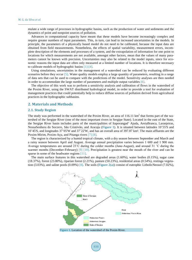
The main surface features in this watershed are degraded areas (1.60%), water bodies (0.15%), sugar cane (18.37%), forest (23.80%), riparian forest (2.21%), pasture (50.23%), residential areas (0.54%), restinga vegeta-tion (3.03%), and saline pools (0.09%) [8]. The soils (Figure 2(a)) consist of eutrophic LitholicNeosol (7.02%),
Figure 1. Location of the watershed of the Poxim River.
M. G. da Silva et al.
839
Quartzarenic Neosol (11.78%), LitholicNeosol (16.67%), Gleysol (10.11%), and Red-Yellow Argisol (54.40%) [8].The slope of the terrain (Figure 2(b)) was described according to the five categories established by [12]. These are flat (0% -3% angle), gentle slope (3% - 8%), slope (8% - 20%), steep slope (20% - 45%), and moun-tainous (>45%).
2.2. Description of the Model The SWAT (Soil and Water Assessment Tool) distributed model was developed by the Agricultural Research Service (ARS) of the United States Department of Agriculture (USDA). It enables prediction of the long-term impacts of soil management practices on the water, sediments, and pesticide levels in large hydrographic basins with different types of soils, land use, and management practices [13]. It was employed by the USDA’s Natural Resources Conservation Service during the Conservation Effects Assessment Project (CEAP), created in 2003 to measure the environmental effects of conservation measures implemented at different spatial scales [14]. SWAT has been widely used to simulate processes that occur in the environment, identify the origins of contaminants, predict the likely outcomes of different scenarios, and establish the causes and effects of diffuse sources of pol-lution [15].
Based on the topographical characteristics of the terrain, obtained from a digital elevation model (DEM), the model delimits watersheds, defines the drainage network, and describes the spatial variability of the hydro-graphic basin, by splitting it into smaller units. The basin is first split into subbasins and the network of channels is calculated. Each subbasin is then divided into hydrological response units (HRUs), which are areas with ho-mogeneous characteristics defined after establishing categories in terms of soil use, soil type, and slope. Based on the options available in SWAT, the HRUs can describe different parts of the subbasin in terms of the main types of soil and land use, as well as management characteristics, and can reflect differences in evapotranspira-tion between different cultivations and soils [13] [16]-[18].
Surface runoff is predicted separately for each HRU, which then enables the determination of runoff in the hydrographic basin as a whole. This procedure improves accuracy and provides a better physical description of the hydric balance [13] [19] [20]. Hence, all the processes that occur in the landscape are modeled for each HRU within the hydrographic basin, independent of its position in the subbasin [21]. The complete cycles of the nu-trients nitrogen and phosphorus in the HRUs can also be modeled using SWAT [13].
(a) (b)
Figure 2. Soil classes (a) and declivity (b) in the watershed of the Poxim River.
M. G. da Silva et al.
840
For each HRU, the volume of surface runoff is simulated using the curve number (CN) method of the Soil Conservation Service [22], which calculates surface runoff as a function of the type and use of the soil, slope, initial soil humidity, and type of management practice [13]. The evapotranspiration potential is determined using the Penman-Monteith equation and is corrected for the type of soil cover and simulated plant growth in order to obtain the real evapotranspiration rate [13] [23].
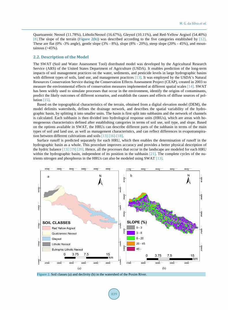
2.3. Input Data The data required for simulation in SWAT concern topography, soil type, land use, and meteorology. A digital elevation model (DEM) was used to provide the topographical data at a resolution of 90 × 90 m (Figure 3(a)).
Although there has been debate concerning the influence of the DEM on the processes simulated by SWAT [24]-[26], the same resolution was also used by [27]-[29], while [30] used a resolution of 100 m. In all cases, SWAT was able to achieve the desired objectives. The DEM utilized was generated from radar data obtained during the Shuttle Radar Topography Mission (SRTM) project [31]. Demarcation of the hydrographic basin, considering the drainage network and the size of the subbasins, employed a minimum channel area of 150 ha [17]. The convergence point of the subbasins was at −10.92 (latitude) and −37.19 (longitude), for which the av-erage daily discharge for the period July 2011 to January 2012 was 1.20 m³∙s−1, with minimum and maximum values of 0.02 and 9.17 m³∙s−1, respectively. Twenty-five subbasins were identified in an overall area of 113.12 km2 (Figure 3(b)).
In order to simulate the area and hydrological parameters within each subbasin, SWAT requires data con-cerning the soil type and land use [32]. Maps of the watershed of the Poxim River containing this information (vegetation type, land use, and soil class), at a scale of 1:400,000, were obtained from the Atlas of Hydric Re-sources of Sergipe [8].
Since the hydric balance is one of the physical processes considered by SWAT, the model requires parameteriza-tion of the soil [33]. Samples were therefore collected and analyzed in order to determine the physical characteris-tics of the soil. The parameters that were not measured were estimated using pedotransfer functions (Table 1).
For definition of the HRUs, limits of 10%, 20%, and 10% were established for soil use, soil type, and slope, respectively. These values have been used previously by [34] [35]. The final number of HRUs was 209. After definition of the HRUs, the soil uses and declivities in the area studied were reclassified by the model, as shown in Table 2.
(a) (b)
Figure 3. Digital elevation model (a) and subbasins (b) of the watershed of the Poxim River.
M. G. da Silva et al.
841
Table 1. Characteristics of the soil in the watershed of the Poxim River.
Variable Parameter in SWAT Value Source
Porosity (%) ANION_EXCL 0.45 - 0.50 Measured
Depth of soil (mm) SOL_Z 150 - 500 Measured
Density of soil (g∙cm−3) SOL_BD 1.52 - 1.75 Measured
Available soil water content (mm H2O mm−1 soil) SOL_AWC 0.03 - 0.42 Measured
Sand (%) SAND 66.01 - 86.89 Measured aEMBRAPA (1997); bFIORIN (2008): pedotransfer function. Table 2. Soil uses and slope classes in the watershed of the Poxim River, after definition of the HRUs.
Soil use Corresponding soil use in the SWAT model Area (%) Slope (%) Area (%)
The climatic data (daily measurements of precipitation, maximum and minimum temperature, solar radiation,
relative humidity of the air, and wind speed) were obtained from the Aracaju meteorological station, operated by the National Meteorological Institute (INMET) (latitude −10.95, longitude −37.04, altitude 4.72 m). The data used were for the period 01/01/1991 to 30/06/2012. Precipitation data were obtained from measurement stations at Itabaiana (latitude −10.70, longitude −37.42, altitude 200 m), São Cristóvão (latitude −10.92, longitude −37.20, altitude 30 m), and Laranjeiras (latitude −10.81, longitude −37.17, altitude 13 m), operated by the Cen-ter for Weather Forecasting and Climate Studies of the National Space Research Institute (CPTEC/INPE), for the period 01 January 2000 to 30 June 2012.
2.4. Performance Evaluation of the Model The performance of the model was evaluated by visual and statistical comparison of the measured and simulated data. The graphical technique provided an initial general overview [36]. Interpretation of the hydrograms first focused on the peak flows and then on the baseflow.
Amongst the various statistical parameters that can be used to evaluate hydrological models, the American Society of Civil Engineers [36] has highlighted the Nash-Sutcliffe efficiency coefficient (NSE) [37]. The statis-tical criteria used here to evaluate the performance of the model are indicated in Table 3.
The NSE describes the deviation from unity of the ratio of the square of the difference between the observed and simulated values and the variance of the observations [38]. The value of the coefficient can vary from minus infinity to one, with the latter value indicating perfect agreement between the simulated and observed data [36]. A smaller NSE value indicates a poorer fit between the simulated and observed time series data. It is possible to obtain negative values of the NSE, indicating that the average of the observational data provides a better fit to the data, compared to the simulated values; in other words, use of the simulated model values is worse than simply using the observed average [39]-[41]. For NSE values that are negative or very close to zero, the predic-tion of the model is considered to be poor or unacceptable [42].
The percent bias (PBIAS) describes the tendency of the simulated data to be greater or smaller than the ob-served data, expressed as a percentage [41]. The optimum PBIAS value is 0.0, and low values indicate that the model simulation is satisfactory. Positive values indicate a tendency of the model to underestimate, while nega-
M. G. da Silva et al.
842
Table 3. Criteria for evaluating the performance of the hydrological model, and their corresponding classifications. i—time series of the measured and simulated pairs; n—number of pairs of the measured and simulated variables; Oi—observational data; Si—simulated data; O —mean of the observational data.
Statistical criterion Value Classification of performance Reference
tive values are indicative of overestimation [43]. This test is recommended due to its ability to reveal any poor performance of the model [44].
The root mean square error (RMSE) provides a measure of the average difference between the measured and simulated values, and can be positive or negative [38]. Values close to 0.0 indicate a perfect fit, with values smaller than half the standard deviation (SD) of the observed values being considered low [45].
The RSR value, which is the ratio of the RMSE to the standard deviation of the observations, can provide ad-ditional information, as recommended by [46], and can be applied to a variety of different constituents [41].
There are no existing standards describing the range of values of the statistical parameters that would indicate acceptable performance of the model [40]. The criteria adopted were therefore based on a review of the litera-ture (Table 3).
3. Results and Discussion 3.1. Sensitivity Analysis of the Model Parameters The parameters used for the flow were selected based on the literature and the SWAT documentation. The initial simulation to determine the sensitivity of the model to different parameters was performed using default para-meter values. The values were then varied within upper and lower limits established according to the characte-ristics of each parameter, using three methods. In the first procedure, the initial value of the parameter is mod-ified by adding an increment. The second method consists of multiplying the initial value by a set amount. In the third method, the initial value is substituted by a different value [47].
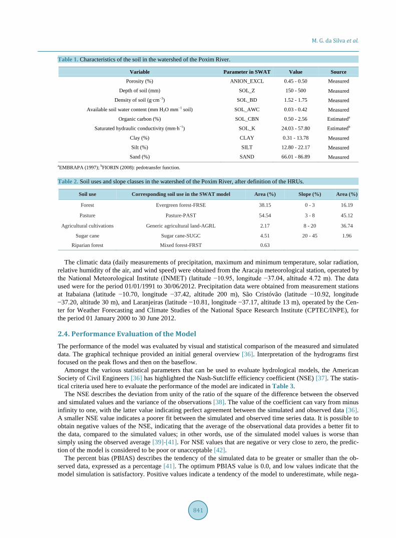
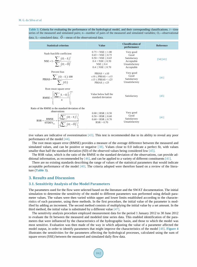
The sensitivity analysis procedure employed measurement data for the period 1 January 2012 to 30 June 2012 to evaluate the fit between the measured and modeled time series data. This enabled identification of the para-meters that were influenced by the characteristics of the hydrographic basin, and those to which the model was most sensitive. Evaluation was then made of the way in which adjusting the value of a parameter affected the model output, in order to identify parameters that might improve the characteristics of the model [48]. Figure 4 illustrates the sensitivities for the parameters affecting the hydrological processes, calculated using the sum of square errors (SSE) between the measured and simulated daily flow data.
M. G. da Silva et al.
843
The sensitivity of the model to a parameter is determined using the percentage difference between the output values of the objective function for simulations performed immediately before and immediately after changing the value of a parameter [48]. A higher value indicates greater sensitivity for a given parameter.
Thirteen of the twenty parameters submitted to sensitivity analysis showed significant effects on simulation of the flow, and were therefore those to which the model was most sensitive. Assignment of the degree of sensitiv-ity is subjective [39]. Here, most of the parameters to which the model was considered to be sensitive were those with average percentage variation of the value of the objective function greater than 0.05 (Figure 5).
3.2. Calibration of the Model Parameters The parameters that influenced the surface runoff and base flow were optimized in the manual calibration. As a way of reducing the number of parameters to be calibrated, ordering of the parameters (Figure 4) was used to select only those for which the sensitivity value was ≥0.05). The calibration was performed using the period 01 January 2012 to 30 June 2012. The changes to the parameter values obtained from the calibration process are listed in Table 4.
The curve number (Cn2) was adjusted for the different land uses, including sugar cane, forest, riparian forest, and pasture. This soil hydric balance parameter enables the model to adjust the soil humidity in order to estimate the surface runoff [49]. It is determined by characteristics of the watershed including the type of soil, hydrologi-cal group, soil use and management, and initial humidity, amongst others, and its value varies from 1 to 100. A completely permeable soil would have a Cn2 value of 1, while a totally impermeable soil would have a Cn2
Figure 4. Results of the sensitivity analysis for the model parameters in terms of the average percentage variation in the value of the objective function.
Figure 5. Hydrogram of the daily flow for the calibration period.
Table 4. Alterations and final parameter values after manual calibration.
Parameters Alteration Final value
Alpha_Bf +0.95 0.998
Canmx +2 2
Ch_K2 +2 2
Cn2 +5% various
Esco +0.95 0.95
Gw_Delay Substituted by 75 75
Gw_Revap Substituted by 0.03 0.03
Slope –5% various
Slusbbsn +5% various
Sol_Awc +10% various
SoL_K +20% various
Sol_Z +5% various
Surlag Substituted by 1 1
value of 100 [50].
High values of Cn2 reflect increased surface runoff and reduced baseflow [51]. The standard Cn2 values de-fined in the manual of the Soil Conservation Service (SCS) were increased by 5%, which increased the surface runoff and provided a better estimate of soil drainage [52] [53]. The alteration was similar to those reported pre-viously [54] [55].
The available water capacity of the soil (Sol_Awc) is the volume of water available to plants when the soil is at field capacity [56]. It can be estimated by determining the quantity of water released between field capacity (water content at a soil water matric potential of −0.033 Mpa) and the point of permanent wilting (water content at a soil water matric potential of −1.5 Mpa) [50], and has an inverse relation with the components of the hydric balance. High values of Sol_Awc signify a high capacity of the soil to maintain its humidity, which reduces the amount of water available for surface runoff and percolation, and therefore affects the production of water [51] [57]. The value of this parameter was increased by 10%, relative to the initial value, in order to obtain conver-gence between the observational and simulated data.
The soil evaporation compensation factor (Esco) adjusts the depth considered for evaporation from the soil, involving capillary action, crusts, and cracks. A low Esco value reflects an ability of the deeper soil layers to compensate the hydric deficit in the upper layers, resulting in greater evapotranspiration, reduced surface runoff and baseflow, and reduced soil water content [51] [56] [58]. The Esco value lies in the range 0.01 - 1.0. When a high Esco value is used in the model, there is less extraction of the evaporative demand from lower levels, so that evaporation is reduced. Here, the value of this parameter was adjusted to 0.95.
The three parameters described above (Cn2, Sol_Awc, and Esco) govern the behavior of surface waters [59], and favor the direct contribution of surface runoff to the flow [60].
The baseflow recession constant (Alpha_Bf) reflects the response of the subterranean flow to changes in re-charge. Calibration of this parameter enables better fitting of the hydrogram [34], and here an increment of +0.95 was added to the standard Alpha_Bf value. According to [13], Alpha_Bf values of between 0.9 and 1.0 are used for soils that show rapid recharge responses, while values between 0.1 and 0.3 are used for soils with slow responses. The importance of the Alpha_Bf parameter is because in dry periods the flow depends on the contribution of subterranean water, which in turn has a strong relationship with Alpha_Bf [47].
The Gw_Revap coefficient describes the quantity of water that moves from the superficial aquifer to the root zone due to the depletion of soil humidity and the direct capture of underground water by the deep roots of trees and bushes [56]. A value near 0.0 reflects restricted movement of water from the superficial aquifer to the root zone, while a value near unity indicates that the transfer rate is close to the rate of evapotranspiration [50]. An
M. G. da Silva et al.
845
increase of the water return coefficient reduces the baseflow due to increased transfer of water from the shallow aquifer to the root zone. The value of this parameter was changed to 0.03.
The Gw_Delay parameter is the delay time for recharge of the aquifer, representing the time required for wa-ter to move from the deepest soil layer (the root zone) and reach the shallow or superficial aquifer [13]. The value of this parameter was changed from 32 to 75. The parameters Alpha_Bf, Gw_Delay, and Gw_ Revap go-vern the response of the subsurface water [59].
The Surlag parameter determines the response of the watershed [56] and provides a storage factor for basins where there is a delay of more than one day before the surface runoff reaches its final convergence point [55]. The value of this parameter was changed from 4 to 1, corresponding to greater storage of water [49]. Delay in the release of surface runoff acts to smooth the simulated flow hydrogram. However, values smaller than 0.5 are not suitable for the release of surface runoff in a subbasin of the main channel [56].
Increase of the Slope parameter increases the lateral flow [52]. The hydraulic conductivity of the channel (Ch_K2) governs the movement of water from the riverbed to the subsoil, or vice-versa, in the case of ephemer-al or transitory rivers [59] [60]. The Sol_Z parameter defines the thickness of the soil layer, influencing the movement of water in the soil during the processes of redistribution and evaporation of soil water [61]. A 5% increase in the value of this variable served to increase the surface runoff.
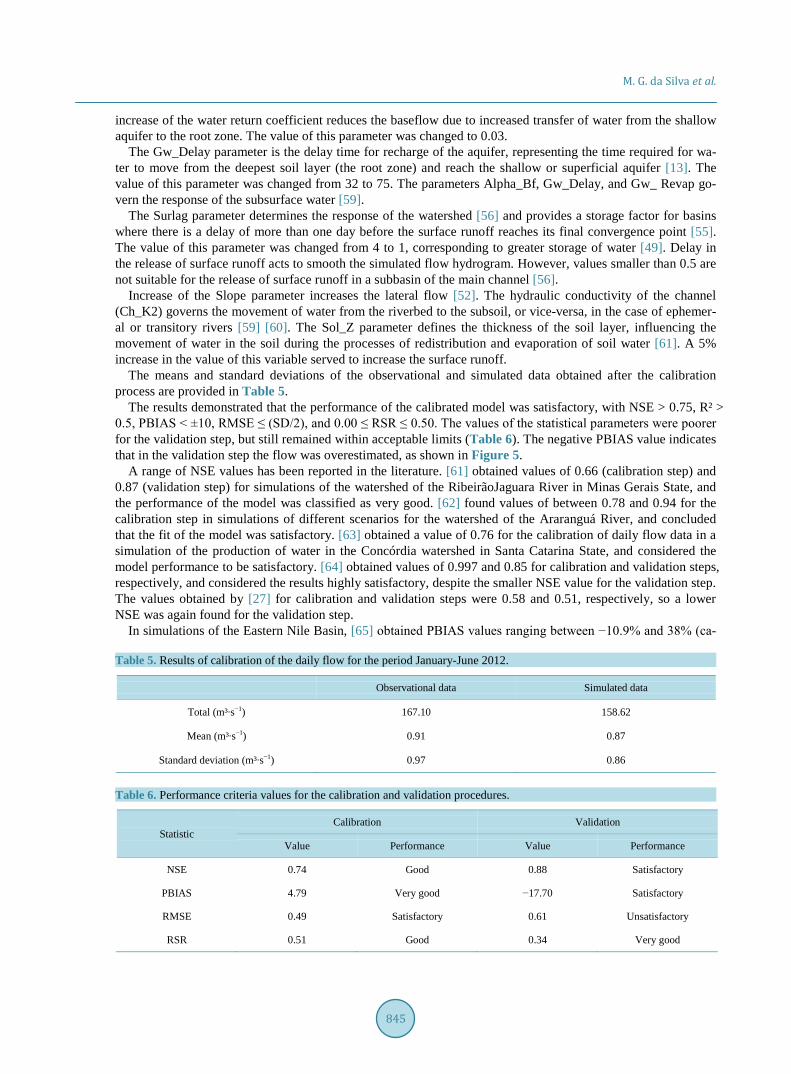
The means and standard deviations of the observational and simulated data obtained after the calibration process are provided in Table 5.
The results demonstrated that the performance of the calibrated model was satisfactory, with NSE > 0.75, R² > 0.5, PBIAS < ±10, RMSE ≤ (SD/2), and 0.00 ≤ RSR ≤ 0.50. The values of the statistical parameters were poorer for the validation step, but still remained within acceptable limits (Table 6). The negative PBIAS value indicates that in the validation step the flow was overestimated, as shown in Figure 5.
A range of NSE values has been reported in the literature. [61] obtained values of 0.66 (calibration step) and 0.87 (validation step) for simulations of the watershed of the RibeirãoJaguara River in Minas Gerais State, and the performance of the model was classified as very good. [62] found values of between 0.78 and 0.94 for the calibration step in simulations of different scenarios for the watershed of the Araranguá River, and concluded that the fit of the model was satisfactory. [63] obtained a value of 0.76 for the calibration of daily flow data in a simulation of the production of water in the Concórdia watershed in Santa Catarina State, and considered the model performance to be satisfactory. [64] obtained values of 0.997 and 0.85 for calibration and validation steps, respectively, and considered the results highly satisfactory, despite the smaller NSE value for the validation step. The values obtained by [27] for calibration and validation steps were 0.58 and 0.51, respectively, so a lower NSE was again found for the validation step.
In simulations of the Eastern Nile Basin, [65] obtained PBIAS values ranging between −10.9% and 38% (ca- Table 5. Results of calibration of the daily flow for the period January-June 2012.
Observational data Simulated data
Total (m³∙s−1) 167.10 158.62
Mean (m³∙s−1) 0.91 0.87
Standard deviation (m³∙s−1) 0.97 0.86
Table 6. Performance criteria values for the calibration and validation procedures.
Statistic Calibration Validation
Value Performance Value Performance
NSE 0.74 Good 0.88 Satisfactory
PBIAS 4.79 Very good −17.70 Satisfactory
RMSE 0.49 Satisfactory 0.61 Unsatisfactory
RSR 0.51 Good 0.34 Very good
M. G. da Silva et al.
846
libration step), and between −25% and 25% (validation step). These values were considered to be good, with the exception of the Abbaysubbasins, where the values were unsatisfactory (±20% < PBIAS ≤ ±40%).
[66] obtained values smaller than ±15%, indicating that the model provided a good simulation of the compo-nents of surface runoff.
[45] reported RMSE values of 0.60 and 0.69 for the calibration and validation, respectively, of daily flow data, indicating an excellent fit between the observational and simulated data. [67] obtained a value of 3.52 for the ca-libration step, and values of 3.45 (year 2000) and 2.24 (year 2001) for the validation step. These values were considered indicative of acceptable simulation of the flow.
A wide range of RSR values have been reported in the literature. [68] obtained values of 0.47 and 0.60 for ca-libration and validation steps, respectively, while [69] obtained values of 0.33 (calibration step) and 0.45 (vali-dation step).
It can be seen from Figure 5 that the simulations slightly underestimated the peak flow values for the Febru-ary to May period, while in June (in the rainy season) the peak flows were slightly overestimated. Nevertheless, the model provided a good simulation of the overall trend in water production. During low water periods, SWAT provided a satisfactory fit, indicating that the model can effectively simulate low flows, as also reported by [61].
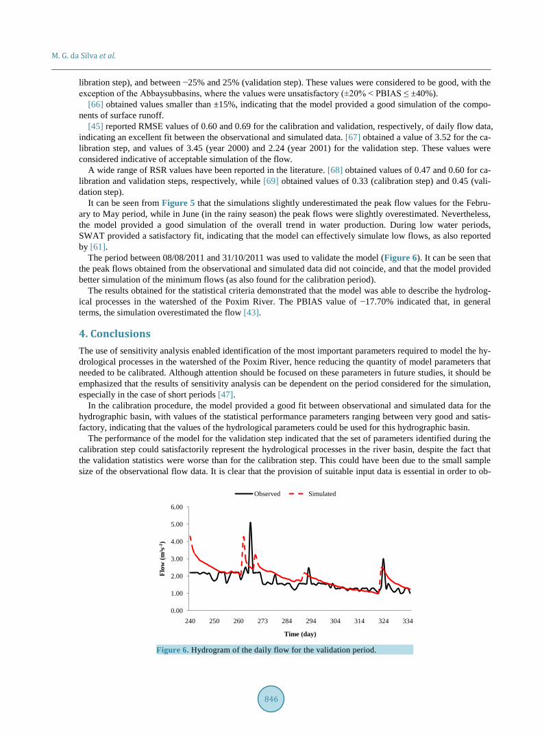
The period between 08/08/2011 and 31/10/2011 was used to validate the model (Figure 6). It can be seen that the peak flows obtained from the observational and simulated data did not coincide, and that the model provided better simulation of the minimum flows (as also found for the calibration period).
The results obtained for the statistical criteria demonstrated that the model was able to describe the hydrolog-ical processes in the watershed of the Poxim River. The PBIAS value of −17.70% indicated that, in general terms, the simulation overestimated the flow [43].
4. Conclusions The use of sensitivity analysis enabled identification of the most important parameters required to model the hy-drological processes in the watershed of the Poxim River, hence reducing the quantity of model parameters that needed to be calibrated. Although attention should be focused on these parameters in future studies, it should be emphasized that the results of sensitivity analysis can be dependent on the period considered for the simulation, especially in the case of short periods [47].
In the calibration procedure, the model provided a good fit between observational and simulated data for the hydrographic basin, with values of the statistical performance parameters ranging between very good and satis-factory, indicating that the values of the hydrological parameters could be used for this hydrographic basin.
The performance of the model for the validation step indicated that the set of parameters identified during the calibration step could satisfactorily represent the hydrological processes in the river basin, despite the fact that the validation statistics were worse than for the calibration step. This could have been due to the small sample size of the observational flow data. It is clear that the provision of suitable input data is essential in order to ob-
Figure 6. Hydrogram of the daily flow for the validation period.
0.00
1.00
2.00
3.00
4.00
5.00
6.00
240 250 260 273 284 294 304 314 324 334
Flow
(m³s
-1)
Time (day)
Observed Simulated
M. G. da Silva et al.
847
tain a good fit between observational and simulated data. The set of parameters identified here could be used for the simulation and evaluation of other scenarios.
Acknowledgements Financial support for this research was provided by the CNPq, IFS and SEMARH/SE.
References [1] El-Nasr, A., Arnold, J.G., Feyen, J. and Berlamont, J. (2005) Modelling the Hydrology of a Catchment Using a Distri-
buted and a Semi-Distributed Model. Hydrological Processes, 19, 573-587. http://dx.doi.org/10.1002/hyp.5610 [2] Eckhardt, K. and Arnold, J.G. (2001) Automatic Calibration of a Distributed Catchment Model. Journal of Hydrology,
251, 103-109. http://dx.doi.org/10.1016/S0022-1694(01)00429-2 [3] Holvoet, K., van Griensven A., Seuntjens, P. and Vanrolleghem, P.A. (2005) Sensitivity Analysis for Hydrology and
Pesticide Supply towards the River in SWAT. Physics and Chemistry of the Earth, 30, 518-526. http://dx.doi.org/10.1016/j.pce.2005.07.006
[4] Lenhart, T., Eckhardt, K., Fohrer, N. and Frede, H.G. (2002) Comparison of Two Different Approaches of Sensitivity Analysis. Physics and Chemistry of the Earth, 27, 645-654. http://dx.doi.org/10.1016/S1474-7065(02)00049-9
[5] Ahl, R.S., Woods, S.W. and Zuuring, H.R. (2008) Hydrologic Calibration and Validation of SWAT in a Snow-Domi- nated Rocky Mountain Watershed, Montana, USA. Journal of the American Water Resources Association (JAWRA), 44, 1411-1430.
[6] vanGriensven, A. (2005) Sensitivity, Auto-Calibration, Uncertainty and Model Evaluation In SWAT2005. http://biomath.ugent.be/ãnn/swathttp://biomath.ugent.be/~ann/swat_manuals/SWAT2005_manual_sens_cal_unc.pdf
[7] Aguiar Netto, A.O., et al. (2007) Cenário dos corpos d’água na sub-bacia hidrográfica do rio Poxim—Sergipe, na zona urbana, e suas relações ambientais e antrópicas. 15th Simpósio Brasileiro de Recursos Hídricos, Rio Grande do Sul, 25-29 November 2007.
[8] Sergipe (2013) Secretaria de Estado do Planejamento e da Ciência e Tecnologia—Superintendência de Recursos Hídricos. Atlas Digital Sobre Recursos Hídricos, Sergipe.
[9] Silva, A.S., Buschinelli, C.C. de A., Rodrigues, I.A. and Machado, R.E. (2001) Índice de sustentabilidade ambiental do uso da água (ISA_ÁGUA): Municípios da região do entorno do rio Poxim, SE. Embrapa Meio Ambiente, Jaguariúna, 46 p. (Boletim de Pesquisa e Desenvolvimento).
[10] Soares, J.A. (2001) O Rio Poxim, processo urbano e meio ambiente. 67 p. Monograph (Specialization in Management of Environmental Hydric Resources), Universidade Federal de Sergipe.
[11] Pinto, J.E.S.S. (2001) Estudos climatológicos em microbacias de clima semi-árido. 8th Encuentro de Geógrafos de América Latina, Santiago, CD-ROM, 373-382.
[12] Embrapa (2006) Sistema Brasileiro de Classificação de Solos. Embrapa Solos, Rio de Janeiro. [13] Neitsch, S.L., Arnold, J.G., Kiniry, J.R. and Williams, J.R. (2011) Soil and Water Assessment Tool: Theoretical Do-
cumentation—Version 2009. Texas Water Resources Institute Technical Report No. 406. Agricultural Research Ser-vice (USDA) & Texas Agricultural Experiment Station, Texas A&M University, Temple.
[14] Mausbach, M.J. and Dedrick, A.R. (2004) The Length We Go: Measuring Environmental Benefits of Conservation Practices. Journal of Soil and Water Conservation, 59, 96-103.
[15] Arnold, J.G. and Fohrer, N. (2005) SWAT 2000: Current Capabilities and Research Opportunities in Applied Water- shed Modeling. Hydrological Processes, 19, 563-572. http://dx.doi.org/10.1002/hyp.5611
[16] Di Luzio, M., Arnold, J.G. and Srinivasan, R. (2005) Effect of GIS Data Quality on Small Watershed Stream Flow and Sediment Simulations. Hydrological Processes, 19, 629-650. http://dx.doi.org/10.1002/hyp.5612
[17] Galván, L., et al. (2009) Application of the SWAT Model to an AMD-Affected River (Meca River, SW Spain). Esti-mation of Transported Pollutant Load. Journal of Hydrology, 377, 445-454. http://dx.doi.org/10.1016/j.jhydrol.2009.09.002
[18] Mulungu, M.M.D. and Munishi, S.E. (2007) Simiyu River Catchment Parameterization Using SWAT Model. Physics and Chemistry of the Earth, 32, 1032-1039. http://dx.doi.org/10.1016/j.pce.2007.07.053
[19] Neitsch, S.L., et al. (2002) Soil and Water Assessment Tool (SWAT) User’s Manual, Version 2000, Grassland Soil and Water Research Laboratory. Blackland Research Center, Texas Agricultural Experiment Station, Texas Water Re-sources Institute, Texas Water Resources Institute, College Station, Texas.
[20] Shen, Z.Y., Gong, Y.W., Li, Y. and Hong, Q. (2009) A Comparison of WEPP and SWAT for Modeling Soil Erosion
of the Zhangjiachong Watershed in the Three Gorges Reservoir Area. Agricultural Water Management, 96, 1435-1442. http://dx.doi.org/10.1016/j.agwat.2009.04.017
[21] White, E.D., et al. (2011) Development and Application of a Physically Based Landscape Water Balance in the SWAT Model. Hydrological Processes, 25, 915-925http://dx.doi.org/10.1002/hyp.7876
[22] USDA Soil Conservation Service (1972) National Engineering Handbook, Section 4, Hydrology. USDA Soil Conser-vation Service, Washington DC.
[23] Monteith, J.L. (1965) Evaporation and the Environment. 19th Symposia of the Society for Experimental Biology, 19, 205-235.
[24] Chaplot, V. (2005) Impact of DEM Mesh Size and Soil Map Scale on SWAT Runoff, Sediment, and NO3—N Loads Predictions. Journal of Hydrology, 312, 207-222. http://dx.doi.org/10.1016/j.jhydrol.2005.02.017
[25] Chaubey, I., Cotter, A.S., Costello, T.A. and Soerens, T.S. (2005) Effect of DEM Data Resolution on SWAT Output Uncertainty. Hydrological Processes, 19, 621-628. http://dx.doi.org/10.1002/hyp.5607
[26] Dixon, B. and Earls, J. (2009) Resample or Not? Effects of Resolution of DEMs in Watershed Modeling. Hydrological Processes, 23, 1714-1724. http://dx.doi.org/10.1002/hyp.7306
[27] Betrie, G.D., Mohamed, Y.A., van Griensven, A. and Srinivasan, A. (2011) Sediment Management Modelling in Blue Nile Basin Using SWAT Model. Hydrology and Earth System Sciences, 15, 807-818. http://dx.doi.org/10.5194/hess-15-807-2011
[28] Bossa, A.Y., et al. (2012) Modeling the Effects of Crop Patterns and Management Scenarios on N and P Loads to Sur-face Water and Groundwater in a Semi-Humid Catchment (West Africa). Agricultural Water Management, 115, 20-37. http://dx.doi.org/10.1016/j.agwat.2012.08.011
[29] Ndomba, P., Mtalo, F. and Killingtveit, A. (2008) SWAT Model Application in a Data Scarce Tropical Complex Cat-chment in Tanzania. Physics and Chemistry of the Earth, 33, 626-632. http://dx.doi.org/10.1016/j.pce.2008.06.013
[30] Pagliero, L., Bouraoui, F., Willems, P. and Diels, J. (2011) SWAT Modeling at Pan European Scale: The Danube Ba-sin Pilot Study. Proceedings of the 2011 International SWAT Conference, Toledo, 15-17 June 2011, 1-14.
[31] Miranda, E.E. (2005) Brasil em Relevo. Embrapa Monitoramento por Satélite, Campinas. http://www.relevobr.cnpm.embrapa.br
[32] Winchell, M., Srinivasan, R. and Di Luzio, J.M. (2009) ArcSWAT 2.3.4 Interface for SWAT2005: User’s Guide. Blackland Research Center: Texas Agricultural Experiment Station, Temple, 465 p.
[33] Romanowicz, A.A., Vancooster, M., Rounsevell, I. and Junese, L. (2005) Sensitivity of the SWAT Model to the Soil and Land Use Data Parameterisation: A Case Study in the Thyle Catchment, Belgium. Ecological Modelling, 18, 27-39. http://dx.doi.org/10.1016/j.ecolmodel.2005.01.025
[34] Boskidis, I., Gikas, G.D., Sylaios, G.K. and Tsihruntzis, V.A. (2012) Hydrologic and Water Quality Modeling of Low-er Nestos River Basin. Water Resource Management, 26, 3023-3051. http://dx.doi.org/10.1007/s11269-012-0064-7
[35] Machado, R.E. (2002) Simulação de escoamento e de produção de sedimentos em uma microbacia hidrográfica utili- zando técnicas de modelagem e geoprocessamento. PhD Thesis, Escola Superior de Agricultura Luiz de Queiroz, São Paulo.
[36] American Society of Civil Engineers (1993) Criteria for Evaluation of Watershed Models. Journal of Irrigation and Drainage Engineering, 119, 429-442. http://dx.doi.org/10.1061/(ASCE)0733-9437(1993)119:3(429)
[37] Nash, J.E. and Sutcliffe, J.V. (1970) River Flow Forecasting through Conceptual Model. Part 1—A Discussion of Prin- ciples. Journal of Hydrology, 10, 282-290. http://dx.doi.org/10.1016/0022-1694(70)90255-6
[38] Feyen, L., V’azquez, R., Christiaens, K., Sels, O. and Feyen, J. (2000) Application of a Distributed Physically-Based Hydrological Model to a Medium Size Catchment. Hydrology and Earth System Sciences, 4, 47-63. http://dx.doi.org/10.5194/hess-4-47-2000
[39] Feyereisen, G.W., Strickland, T.C., Bosch, D.D. and Sullivan, D.G. (2007) Evaluation of SWAT Manual Calibration and Input Parameter Sensitivity in the Little River Watershed. American Society of Agricultural and Biological Engi-neers, 50, 843-855. http://dx.doi.org/10.13031/2013.23149
[40] Loague, K. and Green, R.E. (1991) Statistical and Graphical Methods for Evaluating Solute Transport Models: Over-view and Application. Journal of Contaminant Hydrology, 7, 51-73. http://dx.doi.org/10.1016/0169-7722(91)90038-3
[41] Moriasi, D.N., Arnold, J.G., Van Liew, M.W., Bingner, R.L., Harmel, R.D. and Veith, T.L. (2007) Model Evaluation Guidelines for Systematic Quantification of Accuracy in Watershed Simulations. American Society of Agricultural and Biological Engineers, 50, 885-900.
[42] Santhi, C., Arnold, J.G., Williams, J.R., Dugas, W.A., Srinivasan, R. and Hauck, L.M. (2001) Validation of the SWAT
Model on a Large River Basin with Point and Nonpoint Sources. Journal of the American Water Resources Association, 37, 1169-1188. http://dx.doi.org/10.1111/j.1752-1688.2001.tb03630.x
[43] Gupta, H.V., Sorooshian, S. and Yapo, P.O. (1999) Status of Automatic Calibration for Hydrologic Models: Compari-son with Multilevel Expert Calibration. Journal of Hydrologic Engineering, 4, 135-143. http://dx.doi.org/10.1061/(ASCE)1084-0699(1999)4:2(135)
[44] Rasolomanana, S.D., Lessard, P. and Vanrolleghem, P.A. (2012) Single-Objective vs. Multi-Objective Autocalibration in Modelling Total Suspended Solids and Phosphorus in a Small Agricultural Watershed with SWAT. Water Science and Technology, 65, 643-652. http://dx.doi.org/10.2166/wst.2012.895
[45] Singh, J., Knapp, H.V. and Demissie, M. (2004) Hydrologic Modeling of the Iroquois River Watershed Using HSPF and SWAT. Illinois Department of Natural Resources and the Illinois State Geological Survey. Illinois State Water Survey Contract Report 2004-08. http://www.isws.illinois.edu/pubdoc/CR/ISWSCR2004-08.pdf
[46] Legates, D.R. and McCabe Jr., G.J. (1999) Evaluating the Use of “Goodness-of-Fit” Measures in Hydrologic and Hy-droclimatic Model Validation. Water Resources Research, 35, 233-241. http://dx.doi.org/10.1029/1998WR900018
[47] Van Griensven, A., Meixner, T., Grunwald, S., Bishop, T., Diluzio, M. and Srinivasan, R. (2006) A Global Sensitivity Analysis Tool for the Parameters of Multi-Variable Catchment Models. Journal of Hydrology, 324, 10-23. http://dx.doi.org/10.1016/j.jhydrol.2005.09.008
[48] Veith, T.L. and Ghebremichael, L.T. (2009) How to: Applying and Interpreting the SWAT Auto-Calibration Tools. Proceedings of the 5th International SWAT Conference, Boulder, 5-7 August 2009, 26-33.
[49] Parajuli, P.B. (2010) Assessing Sensitivity of Hydrologic Responses to Climate Change from Forested Watershed in Mississippi. Hydrological Processes, 24, 3785-3797. http://dx.doi.org/10.1002/hyp.7793
[50] Neitsch, S.L., Arnold, J.G., Kiniry, J.R. and Williams, J.R. (2005) Soil and Water Assessment Tool Input/Output File Documentation. Grassland, Soil and Water Research Laboratory, ARS of USDA, Riesel.
[51] Jah, M.K. (2011) Evaluating Hydrologic Response of an Agricultural Watershed for Watershed Analysis. Water, 3, 604-617, http://dx.doi.org/10.3390/w3020604
[52] Abraham, L.Z., Roehrig, J. and Chekol, D.A. (2007) Calibration and Validation of SWAT Hydrologic Model for Meki watershed, Ethiopia. Proceeding of the Conference on International Agricultural Research for Development, Universi-ty of Kassel-Witzenhausen and University of Gottingen, Witzenhausen, 9-11 October 2007, 5.
[53] Benaman, J., Shoemaker, C. and Haith, D. (2005) Calibration and Validation of Soil and Water Assessment Tool on an Agricultural Watershed in Upstate New York. Journal of Hydrologic Engineering, 10, 363-374. http://dx.doi.org/10.1061/(ASCE)1084-0699(2005)10:5(363)
[54] USDA-SCS (1986) Urban Hydrology for Small Watersheds. Technical Release No. 55 (TR-55). USDASCS, Washing- ton DC.
[55] Veith, T.L., Van Liew, M.W., Bosch, D.D. and Arnold, J.G. (2010) Parameter Sensitivity and Uncertainty in SWAT: A Comparison across Five USDA-ARS Watersheds. American Society of Agricultural and Biological Engineers, 53, 1477-1486.
[56] Liew, M.W., Veith, T.L., Bosch, D.D. and Arnold, J.G. (2007) Suitability of SWAT for the Conservation Effects As-sessment Project: Comparison on USDA Agricultural Research Service Watershed. Journal of Hydrologic Engineering, 12, 173-189. http://dx.doi.org/10.1061/(ASCE)1084-0699(2007)12:2(173)
[57] Kannan, N., White, S.M., Worrall, F. and Whelan, M.J. (2007) Hydrological Modelling of a Small Catchmentusing SWAT-2000—Ensuring Correct Flow Partitioning for Contaminant Modeling. Journal of Hydrology, 334, 64-72. http://dx.doi.org/10.1016/j.jhydrol.2006.09.030
[58] Ghebremicael, L.T., Mohamed, Y.A., Betrie, G.D., van der Zaag, P. and Teferi, E. (2013) Trend Analysis of Runoff and Sediment Fluxes in the Upper Blue Nile Basin: A Combined Analysis of Statistical Tests, Physically-Based Mod-els and Landuse Maps. Journal of Hydrology, 482, 57-68. http://dx.doi.org/10.1016/j.jhydrol.2012.12.023
[59] Liew, M.W., Arnold, J.G. and Bosch, D.D. (2005) Problems and Potential of Autocalibrating a Hydrologic Model. American Society of Agricultural Engineers, 48, 1025-1040. http://dx.doi.org/10.13031/2013.18514
[60] Confessor Jr., R.B. and Whittaker, G.W. (2007) Automatic Calibration of Hydrologic Models with Multi-Objective Evolutionary Algorithm and Pareto Optimization. Journal of the American Water Resources Association, 43, 981-989. http://dx.doi.org/10.1111/j.1752-1688.2007.00080.x
[61] Andrade, M.A., Mello, C.R. and Beskow, S. (2013) Simulação hidrológica em uma bacia hidrográfica representativa dos Latossolos na região Alto Rio Grande, MG. Revista Brasileira de Engenharia Agrícola e Ambiental, 17, 69-76. http://dx.doi.org/10.1590/S1415-43662013000100010
[62] Blainski, E., Silveira, F.A., Conceição, G., Garbossa, L.H.P. and Vianna, L.F. (2011) Simulação de cenários de uso do
solo na bacia hidrográfica do rio Araranguá utilizando a técnica da modelagem hidrológica. Agropecuária Catarinense, 24, 65-70.
[63] Perazzoli, M., Pinheiro, A. and Kaufmann, V. (2012) Assessing the Impact of Climate Change Scenarios on Water Resources in Southern Brazil. Hydrological Sciences Journal, 58, 77-87.
[64] Lelis, T.A., Calijuri, M.L., Santiago, A.F., Lima, D.C. and Rocha, E.V. (2012) Análise de sensibilidade e calibração do modelo SWAT aplicado em bacia hidrográfica da região sudeste do Brasil. RevistaBrasileira de Ciência do Solo, 36, 623-634. http://dx.doi.org/10.1590/S0100-06832012000200031
[65] Mengistu, D.T. and Sorteberg, A. (2012) Sensitivity of SWAT Simulated Streamflow to Climatic Changes within the Eastern Nile River Basin. Hydrology and Earth System Sciences, 16, 391-407. http://dx.doi.org/10.5194/hess-16-391-2012
[66] Shi, P., et al. (2011) Evaluating the SWAT Model for Hydrological Modeling in the Xixian Watershed and a Compar-ison with the XAJ Model. Water Resource Management, 25, 2595-2612. http://dx.doi.org/10.1007/s11269-011-9828-8
[67] Mishra, A. and Kar, S. (2012) Modeling Hydrologic Processes and NPS Pollution in a Small Watershed in Subhumid Subtropics Using SWAT. Journal of Hydrologic Engineering, 17, 445-454. http://dx.doi.org/10.1061/(ASCE)HE.1943-5584.0000458
[68] Rathjens, H. and Oppelt, N. (2012) SWAT Model Calibration of a Grid-Based Setup. Advances in Geosciences, 32, 55- 61. http://dx.doi.org/10.5194/adgeo-32-55-2012
[69] Ahmed, S., Farida, D. and Javier, B. (2011) Aplication of the SWAT Model to a Sprinkler-Irrigated Watershed in the Middle Ebro River Basin of Spain. Proceedings of the International SWAT Conference, Toledo, 15-17 June 2011, 135- 150.