Sensitivity Tests of a Two-layer Hydrodynamic Model in the ...

Geophysica (1997), 33(2), 69-98

Sensitivity Tests of a Two-layer Hydrodynamic Model in the Gulf ofFinland with Different Atmospheric Forcings

K. Myrberg

Finnish Institute of Marine Research, P.O.Box 33, FIN-00931, Helsinki, Finland

(Received: April 1996; Accepted: January 1997)

Abstract

A two-dimensional, two-layer baroclinic prognostic hydrodynamic model has been developed andcompared with measurements of surface salinity and temperature, the thickness of the upper mixed layerand water level height. The model’s ability to reproduce the main hydrographic features of the Gulf ofFinland is tested. Special attention is paid to the role of atmospheric forcing. In the first simulation theatmospheric forcing derived from the observations of a single weather station (Kalbådagrund) was used.The results of this simulation were compared with the results of model runs, for which the atmosphericinput was taken from the HIRLAM meteorological model. The accuracy of the results improved when theHIRLAM input was used. However, even the version of the HIRLAM model used, which had a horizontalresolution of 55*55 kilometres, could not accurately enough describe the complicated structure of theatmospheric wind and temperature fields over the narrow Gulf (width ca. 40-150 kilometres).

Key words: two-layer model, sensitivity test, atmospheric forcing

1. Introduction

The Gulf of Finland (GOF) is an estuarine basin in the north-eastern Baltic Seawhere marine hydrophysical features from small-scale vortices up to a large-scalecirculation exist. It is a complicated hydrographic region with a saline water input fromthe Baltic Proper and with a large fresh water input from rivers. Because of the largehorizontal salinity gradients, both density and wind-driven currents play a dominant rolein the circulation. The complicated bottom topography favours the formation ofmesoscale circulation patterns, fronts and eddies. The hydrography of the GOF is alsocharacterized by seasonal variations of stratification. The oblong shape of the GOFleads to complicated atmospheric patterns in terms of a horizontally-inhomogeneousdistribution of surface roughness and thermal forcing. On the other hand, thegeographically limited size makes it possible to cover the area with oceanographicobservations having a dense spatial and temporal resolution.

Published by the Finnish Geophysical Society, Helsinki

K. Myrberg70

During recent decades several two-dimensional and three-dimensional numericalprognostic models have been developed. A review of the Baltic Sea models has beengiven by Svansson (1976) and by Omstedt (1989). Both types of models have beenapplied for determining various aspects of flow patterns, water level variability,temperature and salinity distributions. The first two-dimensional model was developedby Hansen (1956) using linearized barotropic equations, in order to simulate the severeflood which took place in the Netherlands in 1953. Welander (1966, 1968) hasdeveloped several versions of two-dimensional models. Welander (1968) used thelinearized two-dimensional model for studies of the Gulf Stream. O’Brien (1967),O’Brien and Hurlburt (1972) used their nonlinear two-layer, two-dimensional flowmodel for studies of upwellings. Other important two-dimensional approaches havebeen introduced e.g. by Laevastu (1973) and by Heaps (1985). For Baltic Sea studies,several two-dimensional models have been developed. Kowalik (1969, 1972) used abarotropic two-dimensional model. Later on, applications relating to the importance ofthe water exchange between the Baltic Sea and the North Sea were studied (Kowalikand Staskiewicz, 1976; Chilika, 1984; Chilika and Kowalik, 1984). Applications of two-dimensional barotropic models have also been used e.g. by Tamsalu (1967) for TallinnBay, and by Voltizinger and Simuni (1963) and by Laska (1966) for storm-surgeproblems in several parts of the Baltic Sea. Several approaches using two-dimensionalmodels have been made in Finland too. Uusitalo (1960) employed a barotropic modelversion to investigate currents in the Gulf of Bothnia. Sarkkula and Virtanen (1978)applied a two-dimensional model to the Bothnian Bay around the Kokemäenjoki riverfor water management purposes. Jokinen (1977) used a barotropic model for his studiesof the Gulf of Bothnia, while Häkkinen (1980) applied such a model to the whole BalticSea, including the Danish Straits, to calculate water level heights. Myrberg (1992) useda two-dimensional, two-layer linear model for studies of climatological circulation inthe Gulf of Finland and the Gulf of Bothnia.

During the 1970’s three-dimensional model development started actively in manyresearch institutes around the world. The first such model was developed by Bryan(1969), whose model was used for studies of the World Ocean. The model has laterbeen modified many times (Killworth et al., 1991) and the latest modified version is incommon use. Simons (1974) developed a three-dimensional model for the Great Lakesin Canada. Blumberg (1977), Blumberg and Mellor (1987) have developed a three-dimensional model, in which a sigma-coordinate system is used in the vertical direction.This model is also widely used in different institutes. Davies (1980) has used his modelsfor many different areas e.g. for water bodies around the U.K.. Among the numerousthree-dimensional models, the following approaches are also worth mentioning. Müller-Navarra (1983) has carried out simulations for the Baltic Sea and North Sea areas;operational modelling is also an ongoing activity. Backhaus (1985) has developed amodel for the North Sea, but applications to other sea-areas have been made too.Recently, Oberhuber (1993) has constructed an isopycnal ocean circulation model. In

Sensitivity Tests of a Two-layer Hydrodynamic Model in the Gulf of Finland... 71

the Baltic Sea area, many of the abovementioned three-dimensional models have beenused. Simons (1976, 1978) applied his model to the Baltic Sea and studied the role oftopography, stratification and boundary conditions in the wind-driven circulation.Kielmann (1981) continued the studies of currents and water-level heights usingSimons’ model. Funkquist and Gidhagen (1984) have applied Kielmann’s modelversion. Krauss and Brügge (1991), Elken (1994) and Lehmann (1995) have applied theBryan-Cox-Semtner-Killworth free-surface model version (Killworth, 1991) forstudying various aspects of the physics of the Baltic Sea. Klevanny (1994) hasdeveloped a modelling system of two-and three-dimensional models for studyingvarious water bodies: rivers, lakes and seas (including the Baltic Sea). Andrejev andSokolov (1992) and Andrejev et al., (1992) have developed a three-dimensional model,which has been used e.g. for dispersion studies in the Gulf of Finland. In Finland athree-dimensional model has been developed by Koponen (1984). The model has beenused for various types of case studies and for operational use (Koponen et. al., 1994).Tamsalu (1996) has recently developed a three-dimensional isopycnal model for theBaltic Sea, the two-dimensional version of which is studied in this paper.

The reader further interested in modelling is referred to e.g. the followingtextbooks: Nihoul (1982), O’Brien (1986), Nihoul and Jamart (1987) and Kowalik andMurty (1993). All the abovementioned textbooks include both the theoretical and thepractical aspects of oceanographic models of various kinds.

The three-dimensional models are those most used today and also naturally themost complete. However, a hierarchy of models of different orders of complexity is stillneeded to realize the advantages and circumvent the limitations of the various types ofmodels (Davies, 1994). A parallel two-dimensional and three-dimensional coupledhydrodynamic-ecosystem modelling study is an ongoing part of Finnish-Estoniancooperation (Tamsalu and Myrberg, 1995; Tamsalu and Ennet, 1995; Tamsalu, 1996).

In this study a two-dimensional, two-layer baroclinic prognostic model with fullynonlinear hydrothermodynamical equations is used. A look is given at the mainequations of the model. According to Nihoul (1994), the right procedure for deriving arealistic two-dimensional model from a three-dimensional one is by integration of theequations over depth. The derivation of the two-dimensional equations from the three-dimensional ones is shown in detail. The results of the model are compared with CTD-measurements (from 1992) of surface salinity and temperature and of thickness of theupper mixed layer as well as with observations of water level height. The analysis of themodel results is focused on August 1992. This is because at that time there were enoughCTD-data available for the western GOF-northern Baltic Proper area, making it possibleto determine accurate boundary conditions for the model’s open boundary in the west.The model tests were carried out for the upper mixed layer of the sea. Comparison ofthe model results with currents has not been carried out, because the two-dimensionalmodel gives vertically-integrated currents in both layers, while the long-term eulerian

K. Myrberg72

current measurements give currents at 2-3 prescribed levels, from which the verticalintegration of current is difficult to carry out.

The main idea of the paper is the testing of the model’s response to atmosphericforcings of various kinds. Firstly, measured values of atmospheric temperature, windspeed and direction, clouds and humidity from a single weather station over the openpart of the GOF (Kalbådagrund) are used as atmospheric input to the model for thewhole GOF. Secondly, the meteorological input is taken from the HIRLAM (HIghResolution Limited Area Modelling; Machenhauer, 1988, Gustafsson, 1991)atmospheric model. On the other hand, the paper tries to demonstrate to what extent thetwo-dimensional model can produce the main characteristics of the hydrodynamicvariables in the upper mixed layer of the sea.

2. Hydrodynamic baroclinic prognostic two-layer model

The present two-dimensional model is a modified version of the model describedby Tamsalu and Myrberg (1995). In that older version the equations were derived inorder to solve the marine system variables in the upper layer and for the vertically-integrated means of the variables. In the new version the equations are derived for boththe upper and bottom layers. A new feature is an evolution equation for the predictionof water level heights. The corresponding model results are compared with observationsin this paper. The atmospheric input in the older version was taken from a singleweather station, whereas in the present version the effects of the spatial variability ofatmospheric forcing is investigated too. This study tries to present a view of the physicalprocesses occuring on time scales ranging from some hours to several days, whereas inthe study by Tamsalu and Myrberg (1995) mostly the monthly mean values for marinesystem variables were investigated.

2.1 Derivation of the two-dimensional model equations from the three-dimensionalstructure

In the following, the derivation of the two-dimensional equations is shownstarting from the three-dimensional equations presented by Tamsalu (1996).

In the sea there are principally two layers: the upper mixed layer and the lowerstratified layer. In the upper mixed layer of the sea the microturbulence (verticalturbulence) is caused mainly by breaking of the wind waves and by instability of thewind drift. Experimental investigations have shown (see for example Miropolsky, 1981)that outside the boundary layers turbulence is weak and intermittent in character. Takinginto account the different hydrophysics in the different layers, the equations can bewritten in the coordinate system σi i i iz h D= −( ) / , where i=1,2; i=1 represents theupper layer, i=2 the lower stratified layer, ( )D h h h Z1 2 1 2= − = −( ) is the mixed layerthickness; h Z1 = is the sea level oscillation; ( ) ( )D h h H h2 3 2 2= − = − is the thickness


of the lower stratified layer; h2 is the interface between the upper and lower layer,h H3 = is the sea depth. A detailed analysis of the 3D model equations as well as of thenumerical analysis is given by Tamsalu (1996).

According to the system described above, the equations of motion can be writtenas follows:

∂∂ct

L L c Fii i+ + =( )1 2 (1)

The continuity equation is written:

∂∂

∂∂

∂ω∂σ

u Dx

v Dy

i i i i i

i

+ + = 0 (2)

The equation for the vertical variations takes the form:

( )1

0

0

0ρ∂∂σ

ρ ρρ

p gD bi

ii

ii=

−= (3)

( ) ( )b T T S Si i i= − − −α β02

0 (4)

where:

ω ∂δ∂

∂δ∂i i i

ii

iw ux

vy

= − − ; δ σi i i ih D= +

c

u

v

T

S

i

i

i

i

i

=

F

py

by

fv

px

bx

fu

c DI

i

ii

ii

ii

ii

p i i

=

− − −

− − +

1

1

1

0

0

0

0

ρ∂∂

∂δ∂

ρ∂∂

∂δ∂

ρ∂∂σ

L c u vD

u c Dx

v c Dyi i i

i

i i i i i i1

1= + + +∂∂

∂∂

∂∂

∂∂

cx

cy

i i ( )' ' ' '

K. Myrberg74

L cD t D

ci

ii

i

i i

i i

i2

1 1= − +( )' '

ω ∂δ∂

∂∂σ

∂ω∂σ

ci

Here:x is directed to the east, y is directed to the north and z is directed downwards,u v w ci i i i i, , , ,ω represent averaged values, u v w ci i i i i

′ ′ ′ ′′, , , ,ω represent turbulentfluctuations, Ui is the velocity vector with components u vi i, and wi , Ti is thetemperature, T0 is a mean temperature, S i is the salinity, S0 is a mean salinity, p i is thepressure, ρ i is the density, ρ0 is the mean density; b i is the buoyancy, g is theacceleration due to gravity; f is the Coriolis parameter, I is the solar radiation; cp is

the specific heat of water, α is the coefficient of thermal expansion, β is an expansioncoefficient for salinity (for details, see Zilitinkevich, 1991).

2.1.1 Parameterization of turbulent fluxes

The turbulent fluxes are parameterized using traditional turbulent coefficients.

uiciDi Dicix

' ' = −µ∂

∂ ; v c D D c

yi i i ii' ' = −µ ∂

∂ ; ω ν ∂

∂σi i ii

i

c D c' ' = − (5)

Here:µ is the coefficient of macroturbulence, ν( )Ri is the coefficient of microturbulence,Riis the Richardson number, u ci i

' ' , v ci i' ' , ωi ic' ' are ensemble averages.

2.1.2 Boundary conditions

At sea level, where σ1 = 0

u v T q S q Ztxz yz T S1 1

01 1

01 1

01 1

01

1' ' ' ' ' ' ' '; ; ; ;ω τ ω τ ω ω ω ∂∂

= − = − = − = − = (6)

τ τxz yz T Sq q0 0 0 0, , , will be calculated using atmospheric data (see, e.g. Niiler and Kraus,

1977).At the bottom of the sea , where σ2 = 1

u ru v rv T S2 2 2 2 2 2 2 2 2 2 20 0 0' ' ' ' ' ' ' '; ; ; ;ω ω ω ω ω= = = = = (7)

The bottom friction is parameterized as follows: r u v= +−1510 322

22. .

In the coastal area we have:

u v Tn

Sni i

i i= = = =0 0; ∂∂

∂∂

(8)


At the open boundary we have:

∂∂

∂∂

∂∂

un

vn

Tn

Si i ii= = = =0; Γ (9)

where n is normal to the coastline and Γ is experimental data for salinity at the model’sboundary.

2.1.3 The two-layer structure

In the upper mixed layer the hydrodynamic fields can be written as follows:

U U t x y1 1 1= ( , , , )σ ; T T t x y S S t x y1 1 1 1= =( , , ); ( , , ) (10)

Integrating equation (1) over the mixed layer, using (10), we obtain:

∂∂ct

L c F11 1 1+ = (11)

where:

c

u

v

T

S

d10

1

1

1

1

1

1=

∫ σ

L c u vD x

D cx y

D cy

1 1 1 1

11

11

11= + − +∂∂

∂∂

∂∂µ ∂

∂∂∂µ ∂

∂cx

cy

1 1 ( )

F

fv D

fu D

cI e q D

q D

x x

y y

p

hT

S

1

1 1 1 1

1 1 1 1

1

00 1 1

1 1

1=

− − +

− − +

− +

−

π τ

π τ

αρ

γ

/

/

( ) /

/

where:

( )π ∂∂

∂∂x g Z

x xD b1 1 1

12

= +

K. Myrberg76

( )π ∂∂

∂∂y g Z

y yD b1 1 1

12

= +

τ τ τx x xh

10= − ; τ τ τy y y

h1

0= −

q q qT T Th

10= − ; q q qS S S

h1

0= −

I I eoz= −γ - I0 is the solar radiation at the sea-surface, γ is the coefficient of attenuation

of solar radiation.In the lower layer the hydrodynamic fields can be determined as follows:

U U t x y2 2 2= ( , , , )σ ; T T t x y S S t x y2 2 2 2 2 2= =( , , , ); ( , , , )σ σ (12)

Integrating equation (1) over the lower layer using (12) we get:

∂∂ct

L c F22 2 2+ = (13)

where:

c

u

v

T

S

d20

1

2

2

2

2

2=

∫ σ

L c u vD x

D cx y

D cy2 2 2 2

22

22

21= + − +∂∂

∂∂

∂∂µ ∂

∂∂∂µ ∂

∂cx

cy

2 2 ( )

F

fv D

fu D

q D

q D

x x

y y

Th

Sh

2

2 2 2 2

2 2 2 2

2

2

=

− − +

− + +

π τ

π τ

/

/

/

/

( ) ( )π ∂∂

∂∂

∂∂

∂∂

∂∂x g Z

xD H b

xb D

xb H

xc D

xb b2

1 11

12 0 2 2 12

= ++

+ + + −


( ) ( )π ∂∂

∂∂

∂∂

∂∂

∂∂y g Z

yD H b

yb D

yb H

yc D

yb b2

1 11

12 0 2 2 12

= ++

+ + + −

Here we use the relation:

( )2 2200

1

2 2 1 0 2 1

2

b d d b c b bσ

σ σ∫∫ − = −

c const0 1 3= ≅ /

τ τx xh ru2 2= − ; τ τy y

h rv2 2= −

( )τ xh hu u= −2 1 Λ ; ( )τ y

h hv v= −2 1 Λ

( )q T TTh h= −2 1 Λ ; ( )q S SS

h h= −2 1 Λ

Λh Dt

= ∂∂

1 if ∂∂Dt

1 0>

Λh = 0 if ∂∂Dt

1 0≤

The so-called split-up method (Marchuk, 1975) is used to calculate the marinesystem equations. For first-order accuracy in time ( )t t ti i≤ ≤ +1 2/ , the mass transport

(advection and macroturbulence) is calculated. So,

c ct

cit

it

i it

+ − + =1/2

0∆

Λ (14)

For second-order accuracy in time ( )t t ti i+ +≤ ≤1 2 1/ , the other terms of equations

(11) and (13) are calculated:

c ct

Fit

it

it

+ +− =1 1 2/

∆ (15)

where: Λ i is the finite-difference operator of Li .

2.2 Calculation of the thickness of the upper mixed layer and the variation in sealevel

In the present two-dimensional model, the thickness of the upper mixed layer isdependent on space and time and is determined by an evolution equation in thefollowing way:

K. Myrberg78

∂∂

εDt

H Db b

RD

b1 1

1 2 1

= − −−

(16)

The calculation is separated into two different cases: the mixed layer is increasing( / )∂ ∂D t1 0> and the mixed layer is decreasing ( / )∂ ∂D t1 0≤ . For details see Tamsaluand Myrberg (1995). If the mixed layer is increasing, we have:

R q m uD

Ic D

eb bp

D= − + +

−2 1 10

13

1

1 0

0 1

1* αρ γ

γ (17)

q w b q qb T S0 0 1 0 0= ′ ′ = −α β , α α1 1 0= −( )T T , ε =10.

where: m1 is a constant, u* is the friction coefficient.If the mixed layer is decreasing, we have ε = 0 4. and Rb takes the form:

R qb b= 0 (18)

For the water level variation Z an evolution equation is determined:

( )[ ]div u D u H D Zt1 1 2 1+ − = ∂∂

(19)

Finite-difference equations are composed using Mesinger’s (1981) schemes.

3. Main characteristics of the Gulf of Finland hydrodynamics

The Gulf of Finland is a large estuarine basin having no sill with the BalticProper. Its surface area is 29 571 km2, mean depth 37 m and volume 1103 km3. Thelength of the GOF is about 400 km and the width varies between 48-135 km. Thegreatest depth is 123 m (see Falkenmark and Mikulski, 1975, Astok and Mälkki, 1988.)The central gulf is quite deep up to longitude 28 degrees east. The southeastern part issomewhat shallower and the easternmost end of the gulf is very shallow. The southerncoast is rather steep whereas the northern coast is very broken with small islands. TheGOF gets narrow towards the eastern end after the large basin at longitude 28 degreeseast. The Neva bight is a very narrow and shallow area. The topographic features arevery rich and can be expected to have important effects on the circulations of the GOF.

The most striking feature of the hydrography of the GOF is that there is nospecific physical border between the Baltic Sea Proper and the GOF, such as a narrowerpart or a shallower area. A line between the Hanko Peninsula and Osmussaar isconventionally treated as a border (see, e.g. Witting, 1910). In general, fresh water flowsoutwards from the GOF in the surface layer. The fresh water input into the GOF fromrivers is an important factor causing water movements. It is of special importance in


spring, when river runoffs have their annual maximum and, on the other hand, the windand atmospheric pressure gradients are weak. In autumn the fresh water input is smallerand strong southwesterly winds dominate. There is then on average an inflow of wateralong the southern coast and an outflow along the northern coast. The salty water fromthe Baltic Proper tends to penetrate into the GOF along the bottom. In the westernmostGOF near the Estonian coast there is a quasistationary salinity front close to the bottom.It has been estimated that the water in the GOF is renewed approximately every threeyears. The amount of fresh water coming in as river runoff is on average 114 km3yearly. This is about 25 percent of the whole fresh water input to the Baltic Sea, whichshows how diverse the water masses of the GOF are. In general it can thus be concludedthat the GOF is characterized by two water exchange processes; one at each end: theexchange with the Baltic Proper in the west, and the largest single fresh water input tothe whole Baltic Sea from the river Neva, with a monthly mean discharge of 2700 m3/s,in the east. The Neva dominates the physics at the eastern end of the GOF. The Nevadischarge has a large yearly variability. In 1992, the year whose data are used in thispaper, the minimum runoff of the River Neva was 1490 m3/s in January, while themaximum runoff was 3610 m3/s in June. Other rivers (Kymi, Narva, Luga) on bothsides of the eastern GOF contribute to the fresh water supply as well. The Kymi andNarva rivers both have a yearly mean runoff of 300-400 m3/s, while that of the Luga isabout 100 m3/s. The role of other rivers is negligible. The hydrography of the GOF isalso modified by air-sea-interaction (wind stress, heat and vapour exchange), barocliniceffects (fronts), bottom topography, coastal effects and by the coriolis-effect. Thecirculation physics of the GOF have been studied in detail e.g. by Witting (1912),Palmén (1930), Hela (1952) and Sarkkula (1989).

It should be pointed out that salinity plays an important role in the buoyancy-driven currents in the Baltic Sea, whereas in the oceans temperature differences makelarger contributions to buoyancy (see e.g. Mälkki and Tamsalu, 1985). This is the reasonwhy special attention is paid in this study to a detailed analysis of the distribution ofsalinity.

4. Material and methods

4.1 Initial conditions, data and parameter values

Before the main simulations the model was initialized in the following way.Firstly, a climatological structure of salinity and temperature was given for the upperlayer and for the bottom layer (Bock, 1971). After that a simulation of 5 years wascarried out using realistic atmospheric, river water and water level input in order to besure that the model had adapted to the real conditions of the year 1992 as well as to seethat the model’s numerical scheme was stable. Each of the simulations described laterin this section was started using the abovementioned initial conditions, which are the

K. Myrberg80

result of this 5 years’ simulation. The main simulation period was from April 15 toSeptember 3, 1992, when the measurements ended. It should be pointed out that theconclusions about the model simulations are based not only on the figures shown, butalso on many other results not shown in this paper.

The monthly mean runoffs of the main rivers in the Gulf of Finland (Neva, Narva,Kymi, Luga) were used. The runoffs of the small rivers were added to the previously-mentioned river runoffs. Using the runoff data, Fourier coefficients were calculated todescribe the time-dependency of river runoff.

In the first simulations, atmospheric data (6h intervals) from the automaticweather station of Kalbådagrund (59 deg. 58 min.N, 25 deg. 37 min.E) were used. Thefollowing meteorological parameters were used: wind speed and direction, atmospherictemperature, relative humidity and total cloudiness. Since cloudiness is not observed atKalbådagrund, which is an automatic weather station, the values from the Isosaariweather station (60 deg. 07 min.N, 25 deg. 03 min.E) were used. The wind is measuredat a height of 35 m. A 10 m wind speed was calculated according to the logarithmicwind law. In the latter simulations, input from the HIRLAM atmospheric model wasused (see section 4.2).

The model simulations were mainly focused on August 1992, when 130 CTDobservations were carried out on board R/V Aranda using a Neil Brown Mark III sonde.Unfortunately, during that year no current measurements were carried out by the FinnishInstitute of Marine Research (FIMR). From the CTD measurements in the transitionarea between the Baltic Proper and the Gulf of Finland (longitude 22 deg.E), theboundary conditions for surface and bottom salinity were calculated. The measuredwater levels at Hanko and Heltermaa were used for assimilation of the water level onthe western boundary of the model. The ability of the model to forecast water levels inother parts of the GOF was tested by comparing the model results with the water levelobservations from Helsinki and Hamina.

No current measurement field experiments were carried out in FIMR during 1992.The current measurement campaigns have been concentrated in the years 1994-1996.These current profiles will be later compared with the results of the three-dimensionalmodel version (Tamsalu, 1996). Current measurements have been carried out during the1990’s in the Finnish Environmental Agency (J. Sarkkula, personal communication).However, the data have not yet been published.

The following model parameters were used in all simulations: grid stepdx=dy=4663 m, time step dt=10 min, bottom friction R u v= +−15 10 3

22

22. * * ,

coefficient of macroturbulence µ = −1 10 3 4 3* * /dx , coriolis-parameter f = 2ω ϕsin ; anddrag-coefficient ( )C Ud = +0 63 0 066 10. . * , where U10 is the wind speed (m/s) at aheight of 10 metres, ϕ is the latitude (rad), ω is the angular velocity of the earth'srotation (rad s-1).


4.2 The use of meteorological forcing from the HIRLAM model

The atmospheric model used in this paper is known as HIRLAM (HIghResolution Limited Area Modelling). This originally joint Nordic-Dutch model wasdeveloped in the 1980's (Machenhauer, 1988). The HIRLAM1 version has been inoperational use in the Finnish Meteorological Institute (FMI) since January 1, 1990.Operational use of the HIRLAM2 version began in the FMI on June 1, 1994. TheHIRLAM1 model version (Gustafsson, 1991) has a horizontal resolution of 0.5 degrees(latitude) and 1.0 degrees (longitude), which translates to about 55*55 km in the BalticSea area. The HIRLAM1 version has about 30 vertical levels. During 1995 a modelversion with a resolution of about 25*25 km was brought into use in the FMI.

The output fields (6h forecasts) from the HIRLAM model (wind speed anddirection, atmospheric temperature) were further modified to be usable for the seamodel. An areal interpolation was carried out in order to place the HIRLAM data on thegrid of the sea model (Cheng and Launiainen, 1993). The horizontal resolution of thesea model is about 5 minutes (longitude) and 2.5 minutes (latitude), which means about4.5*4.5 kilometres. The interpolated HIRLAM winds from the lowest model level,namely at a height of 32-35 m, were compared with the measured winds atKalbådagrund (35 m height), which is nowadays the only true open-sea station in theGOF. The comparisons showed that the modelled winds speeds were in general lowerthan those observed (Fig. 1A). This difference can most probably be explained by thelack of resolution of the HIRLAM model. The model can not "see" the Gulf of Finland.The areal interpolation of the winds also causes some reduction of the speeds, becauseHIRLAM grid points near the coast are used in this procedure. The total number of gridpoints used is only about 15.

A simple correction to the interpolated HIRLAM winds speeds for the whole year1992 is carried out. The corrections to the HIRLAM wind fields only affect wind speed.Corrections to wind direction are too complicated, and besides, the wind direction ismainly determined by the surface pressure pattern, which is well enough forecasted bythe HIRLAM model (Fig. 1A). Atmospheric temperature corrections are not carried outbecause of the lack of observations over the open sea needed to describe thecomplicated temperature pattern.

K. Myrberg82

Fig. 1. The time evolution of wind speed in m/s (A) and wind stress (B) in m s2 2/ during August 1-31,1992 at the Kalbådagrund weather station in the Gulf of Finland. The measured wind speeds and windstresses at Kalbådagrund are marked with continuous lines, the interpolated HIRLAM parameters withdash-dotted lines, and the corrected (by Eq. 20) interpolated HIRLAM parameters with dashed lines.

4.2.1 Corrected HIRLAM wind fields

A regression analysis is used to correct the HIRLAM wind speeds by taking themeasured winds speeds at Kalbådagrund as the correct values. Measurements at 6h


intervals at Kalbådagrund (00, 06, 12, 18 GMT) are used to correct the correspondingHIRLAM wind fields. The following first-order regression equation employed is

U a a UcorrHIRLAM HIRLAM= +0 1 (20)

where: U HIRLAM is the original HIRLAM wind speed (m/s), UcorrHIRLAM is the corrected

HIRLAM wind speed (m/s), a0=1.0, a1=1.5.The original HIRLAM winds at the location of Kalbådagrund are corrected using

(20). The results are shown in Figure 1A. The corrected HIRLAM winds are quiteaccurate. The mean ratio K between the wind stress calculated from the Kalbådagrundwinds and that calculated from the interpolated HIRLAM winds has been determinedusing the wind data of every 6h. K found to be 4. If the corrected interpolated HIRLAMwinds are used, K equals 1.1, which means that at least the mean wind stress is accurate.(Fig. 1B).

The HIRLAM wind fields discussed here are from a height of about 35 m. The10 m winds are calculated from the 35 m winds as follows (T. Vihma, personalcommunication):

U Um m10 350 9= . if Ri≤0 (21a)

U Ri Um m10 350 9 0 5= −( . . ) if Ri≥0 (21b)

where:Ri, the non-dimensional Richardson number, is given by:

Ri gZT

T TUm

m s

m= −

35

35

352

( ) (22)

Here, U35 (m/s) is the corrected HIRLAM wind speed at a height of 35 m, U10is the calculated HIRLAM wind speed at a heigth of 10 m, T m35 (degrees K) is theHIRLAM air temperature at a heigth of 35 m and Ts is the sea-surface temperaturecalculated by the sea model, Z=35 m.

Products of relative humidity and total cloudiness are not easily available fromHIRLAM. So, those values measured at a single station have also been used throughoutthe HIRLAM simulations.

According to Launiainen and Saarinen (1982) there can be major differencesbetween the wind speeds in an open sea-area and in the coastal area. The wind directionaffects the differences of wind speed between coastal and open sea-areas throughvariable roughness and orographic effects. The atmospheric surface layer stability alsoaffects the wind speed differences. Due to the low resolution of the model, theHIRLAM winds for open-sea and coastal areas do not differ much from each other. It is

K. Myrberg84

therefore possible that the interpolated HIRLAM winds in the coastal areas, when thecorrection by (20) has been made, are slightly overestimated compared with the realwinds there. However, use of the interpolated HIRLAM winds in coastal areas iscertainly more realistic than using the space-independent winds from Kalbådagrund. Onthe other hand, the interpolation procedure slightly decreases the HIRLAM winds in theopen sea-area compared with the HIRLAM winds in the original grid system.

4.3 Weather conditions in the Gulf of Finland in August 1992

At the beginning of August (Helminen, 1992) a weak high pressure centre waslocated south of Finland and the weather was clear but not very warm. The airtemperature at Kalbådagrund varied between 13-20 °C, while the wind speed there wasbetween 5-10 m/s, with the wind blowing on average from the west. Between 4 and 7August two frontal systems moved over Finland. In connection with this, high winds ofbetween 10-17 m/s from the west were observed. The weather remained quite warmduring this period. Between 8 and 10 August the weather was relatively cold with lightwinds from the northwest. On August 10 very warm air was advected to Finland andrecord temperatures for summer 1992 were achieved on August 11. Light southerlywinds were observed. After that, the weather became cooler and high winds of up to 20m/s from the southwest were observed on August 13. Temperatures fell from more than25 °C on August 11 down to 11 °C on August 20. The diurnal temperature variabilitywas small. After August 20 a high pressure centre formed over Finland, but the weatherwas cold and cloudy with moderate northerly winds. During the last part of the monththe weather was quite changeable. On August 24 and 28 frontal systems arrived inFinland from the west and the wind direction varied between east and west. Windspeeds were usually below 10 m/s, occasionally being 12-14 m/s. Temperatures werenear 14 °C and the diurnal variability of temperature was small. During the last days ofAugust a weak high pressure centre formed over Finland. Winds turned from westerlyto easterly and advection brought warm air from the east.

5. The model simulations

5.1 Comparison of the model results with different meteorological forcings

In this section the model results for salinity, temperature, the thickness of theupper mixed layer and water level height will be compared with measurements. Thefirst model version, in which atmospheric forcing derived from Kalbådagrundobservations is used, will be referred to the 2DK-model. The second model version, inwhich the air temperature and wind stress fields are obtained from the HIRLAM model,will be referred to the 2DH-model.


5.1.1 Surface salinity fields

The overall horizontal structure of salinity given by the 2DK model (Fig. 2A) isgenerally in accordance with measurements. The surface salinity varies from about 6.5PSU in the southwestern part to about 0.5 PSU in the mouth of River Neva. The effectsof fresh water input from the Kymi, Narva and Luga rivers are also clearly visible. Inthe western part of the Gulf the errors in the 2DK prognoses are of the order of ±0 2.PSU (Fig. 2A). In the eastern part of the central Gulf the 2DK model (Fig. 2A) givessalinities which are systematically about 0.7-1.0 higher than the measurements. In thewestern part of the central Gulf the 2DK model overestimates the salinity by 0.4-1 PSU.In the eastern Gulf the model overestimates the salinity by about 1 PSU.

The 2DH model gives better results than the 2DK model in all parts of the Gulf(Fig. 2B; see section 5.1.3). In the eastern part of the central Gulf the 2DH model givesvery good results with errors of ±0 2. PSU. In the western part of the central Gulf anoverestimation of 0.1-0.7 PSU is still evident even in the 2DH-model. The mostpronounced differences between the 2DH and 2DK models are in the eastern Gulf ofFinland, where the 2DK model (Fig. 2A) gives e.g. on August 18 a value of 3.5 PSU,while the 2DH model (Fig. 2B) gives 2.7 PSU. The measured value at that point (stationF40; 60 deg. 06 min.N, 28 deg. 48 min.E.) was 2.3 PSU.

The time evolution of salinity in the western part of the GOF (station GR6, 59deg. 41 min.N, 23 deg. 34 min.E), shows the role played by the fixed values for salinityat the model’s western boundary (not shown). The surface salinity variability accordingto the model results is less than that shown by measurements.

5.1.2 Surface temperature fields

Surface temperature fields simulated by the 2DK model (Fig. 3A) show that thehorizontal temperature gradients are very small. This can be simply explained by thefact that the spatial variability of air temperature was not taken into account (see section4.1-4.2). The 2DK model overestimates the surface temperature up to the middle ofAugust by about 0.5-1.5 degrees. During the second half of August the modelunderestimated the temperature by about 1-2 degrees (Fig. 3A), even by as much as 4degrees on August 22. The model’s ability to describe the sea-surface temperature isthus only moderate if atmospheric input from a single point is used.

K. Myrberg86

Fig. 2. Surface salinity fields in the Gulf of Finland. (A): simulated by the 2DK model version using theatmospheric forcing derived from the Kalbådagrund weather station and (B): simulated by the 2DH modelversion using the atmospheric forcing from HIRLAM. The figures represent the mean of model resultsfrom August 18-21. Positions of the salinity measurements carried out between August 18-21 are markedwith a black dot (according to model results changes in the horizontal salinity field were small duringAugust 18-21). The isoline analysis of the model results is shown at intervals of 0.2 PSU and the scale ofthe corresponding colours are shown below.

The 2DH model results show more pronounced sea temperature gradients thanthose from the 2DK. However, the simulated sea temperature results of the 2DH modelare not much more accurate than the 2DK model results (Fig. 3B; see section 5.1.3). Atthe beginning of August (up to August 5) the 2DH model overestimates thetemperatures by about 0.3-1 degrees. After that, up to August 15, the 2DH model resultshave errors of about ±1 degrees. In late August the 2DH model overestimates thetemperature by about 1-2 degrees.

The time-evolution of sea temperature in the upper mixed layer at station LL9 (59deg. 42 min.N, 24 deg. 02 min.E) from early May up to the beginning of Septembershows that the 2DH model is capable of reproducing the seasonal time evolution oftemperature in the GOF (not shown). The large error in the model results around May20 can be explained by the difficulties in the determination of the evolution of the upper


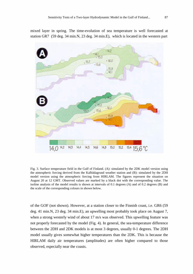
mixed layer in spring. The time-evolution of sea temperature is well forecasted atstation GR7 (59 deg. 34 min.N, 23 deg. 34 min.E), which is located in the western part

Fig. 3. Surface temperature field in the Gulf of Finland. (A): simulated by the 2DK model version usingthe atmospheric forcing derived from the Kalbådagrund weather station and (B): simulated by the 2DHmodel version using the atmospheric forcing from HIRLAM. The figures represent the situation onAugust 20 at 12 GMT. Observed values are marked by a black dot with the corresponding value. Theisoline analysis of the model results is shown at intervals of 0.1 degrees (A) and of 0.2 degrees (B) andthe scale of the corresponding colours in shown below.

of the GOF (not shown). However, at a station closer to the Finnish coast, i.e. GR6 (59deg. 41 min.N, 23 deg. 34 min.E), an upwelling most probably took place on August 7,when a strong westerly wind of about 17 m/s was observed. This upwelling feature wasnot properly forecasted by the model (Fig. 4). In general, the sea-temperature differencebetween the 2DH and 2DK models is at most 3 degrees, usually 0-1 degrees. The 2DHmodel usually gives somewhat higher temperatures than the 2DK. This is because theHIRLAM daily air temperatures (amplitudes) are often higher compared to thoseobserved, especially near the coasts.

K. Myrberg88

Fig. 4. Time evolution of temperature in the upper mixed layer at station GR6 (59 deg. 41 min.N, 23 deg.34 min.E). The continuous line represents results as simulated by the 2DH model, the broken line those ofthe 2DK model.

5.1.3 Statistical analysis

A statistical analysis was carried out in order to investigate how reliable the modelresults are compared with observations, and besides this to see whether the use of theHIRLAM atmospheric model has any effect in reducing the errors of model resultscompared with observations. The statistical error R (as a percentage) is defined asfollows:

Rabs F F n

F

MO ME ii

n

ME

=−

=∑

100 1( ) /

_ (23)

F F nME ME ii

n=

=∑ ( ) /

1

where:

R is the error as a percentage, FME is the value of the measured variable (surfacesalinity or temperature) at an observational point, FMO is the value of the variablesimulated by the model at the same location, FME is the mean of all the observations of


the variable in the studied area, n is the number of observations (n=130 for the wholeGOF).

In Tables 1A and 1B, the errors have been given for surface salinity andtemperature found when using the 2DK and the 2DH models. The errors have beencalculated separately for the western GOF, the central GOF, the eastern GOF and for thewhole GOF. The number n in (23) is here the number of observations in thecorresponding sea-area.

Table 1a. The error R (as a percentage) in surface salinity simulations produced by the 2DK and the 2DHmodels for various parts of the GOF: the western GOF, the central GOF, the eastern GOF and the wholeGOF.

WGOF CGOF EGOF whole GOF

2DK 2.5 13.1 27.5 7.32DH 2.0 6.0 10.0 4.0

Table 1b. The error R (as a percentage) in surface temperature simulations produced by the 2DK and the2DH models for various parts of the GOF. In temperature calculations the Celsius scale has been used.

WGOF EGOF CGOF whole GOF

2DK 5.3 7.6 8.3 6.02DH 4.2 6.7 8.3 5.6

The statistical error analysis shows clearly that the 2DH model gives better resultsfor surface salinity than 2DK (errors 4.0 % versus 7.3 %). The difference between thesemodels is smallest in the westernmost GOF (2.0 % versus 2.5 %) because the salinityhas a constant value at the western boundary. The difference in accuracy between the2DK and the 2DH models’ salinity simulations increases eastwards, because thedominating effect of the fixed western boundary is not important, besides which thereare large salinity gradients in the central (errors 6.0 % versus 13.0 %) and the easternGOF (errors 10.0 % versus 27.5 %), which can be predicted accurately only making useof the HIRLAM input.

The error analysis of surface temperature between the 2DK and the 2DH modelsshows no major difference in accuracy. The 2DH model is more accurate than the 2DKmodel (error for the whole of the GOF; 5.6 % versus 6.0%), except in the eastern part,where the results are equally accurate.

5.1.4 Thickness of the upper mixed layer

The results of the 2DK and the 2DH models for the thickness of the upper mixedlayer are so similar that only the latter case is analyzed here. The model seems to beable to predict the mixed layer thickness in the open sea-area, where the errors in modelresults are about ±3 metres. However, rapid changes in the thickness of the upper mixed

K. Myrberg90

layer caused by upwellings, or by considerable cooling/warming in the atmosphere,cannot be forecast accurately. This is due partly to shortcomings in the model physics.In the model the upper mixed layer never vanishes, whereas during an upwelling theupper layer in fact does vanish (Hela, 1976). Thus, problems in determining thethickness of the upper layer are most pronounced near the coasts. To some extent theerrors are also caused by inaccuracies in the atmospheric forcing. Figures 5A, B showhow the water body in the eastern GOF becomes well-mixed between August 18-20 dueto a cold air outbreak and its corresponding northerly winds (Fig. 1A; see section 4.3).This mixing seems to have some observational support.

Fig. 5. Fields of the thickness of the upper mixed layer in the Gulf of Finland simulated by the 2DHmodel version. The figures represent the situation at 12 GMT each day: August 18 (A), August 20 (B).Observed values are shown by a black dot with the corresponding value. The isoline analysis of the modelresults is shown at intervals of 2 metres.


5.1.5 Currents and water level

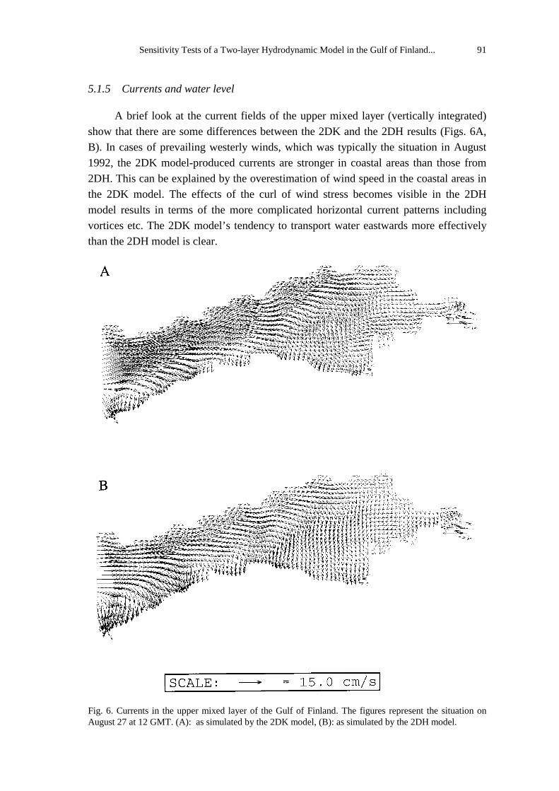
A brief look at the current fields of the upper mixed layer (vertically integrated)show that there are some differences between the 2DK and the 2DH results (Figs. 6A,B). In cases of prevailing westerly winds, which was typically the situation in August1992, the 2DK model-produced currents are stronger in coastal areas than those from2DH. This can be explained by the overestimation of wind speed in the coastal areas inthe 2DK model. The effects of the curl of wind stress becomes visible in the 2DHmodel results in terms of the more complicated horizontal current patterns includingvortices etc. The 2DK model’s tendency to transport water eastwards more effectivelythan the 2DH model is clear.

Fig. 6. Currents in the upper mixed layer of the Gulf of Finland. The figures represent the situation onAugust 27 at 12 GMT. (A): as simulated by the 2DK model, (B): as simulated by the 2DH model.

K. Myrberg92

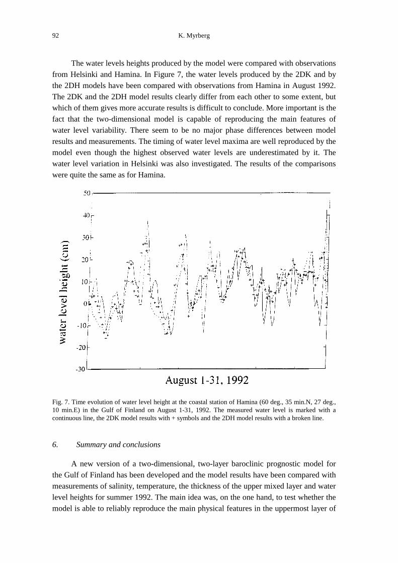
The water levels heights produced by the model were compared with observationsfrom Helsinki and Hamina. In Figure 7, the water levels produced by the 2DK and bythe 2DH models have been compared with observations from Hamina in August 1992.The 2DK and the 2DH model results clearly differ from each other to some extent, butwhich of them gives more accurate results is difficult to conclude. More important is thefact that the two-dimensional model is capable of reproducing the main features ofwater level variability. There seem to be no major phase differences between modelresults and measurements. The timing of water level maxima are well reproduced by themodel even though the highest observed water levels are underestimated by it. Thewater level variation in Helsinki was also investigated. The results of the comparisonswere quite the same as for Hamina.

Fig. 7. Time evolution of water level height at the coastal station of Hamina (60 deg., 35 min.N, 27 deg.,10 min.E) in the Gulf of Finland on August 1-31, 1992. The measured water level is marked with acontinuous line, the 2DK model results with + symbols and the 2DH model results with a broken line.

6. Summary and conclusions

A new version of a two-dimensional, two-layer baroclinic prognostic model forthe Gulf of Finland has been developed and the model results have been compared withmeasurements of salinity, temperature, the thickness of the upper mixed layer and waterlevel heights for summer 1992. The main idea was, on the one hand, to test whether themodel is able to reliably reproduce the main physical features in the uppermost layer of


the GOF, and on the other hand to see what the effect of using space-dependent andspace-independent atmospheric forcings is on the results of the marine hydrodynamicmodel.

The simulations of surface salinity showed satisfactorily the complicatedhorizontal structure with pronounced gradients. The fixed boundary values for salinityin the west became visible in the model results as too small a variability of salinitycompared with measurements. The problem with open boundaries is a clearshortcoming in all regional models and leads to some limitations in their use. Theemployment of input from the HIRLAM atmospheric model clearly improved the modelresults in the eastern GOF. It is probable that the HIRLAM space-dependent wind fieldsbetter describe the situation over the eastern GOF than do the open sea winds of theKalbådagrund weather station; strong westerly winds there cause too much eastwardwater transport and too strong mixing. As a result, the thin fresh water layer vanishesand the model overestimates the surface salinity. Due to the large fresh water input fromthe rivers, large horizontal gradients occur in the eastern GOF, so that the exact locationof the fronts is sensitive to atmospheric forcing.

In the temperature simulations, the seasonal time-evolution of surface layertemperature was fairly well simulated by the model. However, there are cleardifferences between the 2DK and the 2DH models’ results concerning horizontal fieldsof temperature. In the 2DK results, the horizontal variation of surface layer temperaturewas negligible, while in the 2DH results major gradients became visible. This is simplya consequence of the use of the spatially-variable atmospheric temperature in the lattersimulation. However, the accuracy of the 2DH model results when compared withmeasurements is only slightly better than that of the 2DK model. This can be explainedby the lack of resolution in the atmospheric model to describe the air temperaturepattern accurately enough over the sea-area.

To some extent the thickness of the upper mixed layer can be predicted by themodel over the open sea-area, but the consequences of local upwellings,warming/cooling of the atmosphere etc. are difficult to simulate with the two-dimensional model. The correct time and place of the production of a well-mixed sea inlate August is difficult to reproduce and with it a forecast of the related abrupt changesin surface temperature and salinity. A proper modelling of upwelling needs a 3D model,in which the vertical velocity is calculated.

The current fields showed some interesting differences between the 2DK and the2DH model results. When typical westerly winds dominate, the 2DK model seems toproduce higher currents than the 2DH model in coastal areas, which is to be expected,because the wind measurements from Kalbådagrund overestimate the wind speed at theshoreline as well as in the eastern GOF. Thus the 2DK model also has a tendency toproduce higher eastward current speeds in the eastern GOF than the 2DH model. Thisleads to an overestimation of surface salinity there. The overall time evolution and mainpeaks of the water level variations can be described by the present model. Atmospheric

K. Myrberg94

forcing seems to play a certain role, but it is probable that the wind field at theshorelines is not so well described by the HIRLAM model that it could have a positivesignal in the model results. The data-assimilation of water levels at the mouth of theGOF plays a crucial role in the models’ ability to produce reliable water levels in thecoastal areas of the GOF.

This study has shown that atmospheric models need still higher horizontalresolution in such narrow gulfs as the Gulf of Finland in order to describe the wind andtemperature fields accurately. Today, the Finnish Meteorological Institute uses a versionof the HIRLAM model in which the horizontal resolution is about 25*25 km. Hopefullythis atmospheric input can soon be used in sea models.

The two-dimensional model has shown some possibilities for reproducing themain features of the hydrodynamics of the Gulf of Finland. In the near future the resultsof the two -and three-dimensional models will be compared with each other and withmeasurements in order to find out the main differences between the results of modelsrepresenting a different order of complexity.

Acknowledgements

I would like to thank D.Sc. Rein Tamsalu for his guidance of this work and for hiscomments on the manuscript. I extend my appreciation to Dr. Timo Vihma for helpingme in the surface parameterization of the HIRLAM winds, and to Mr. Kalle Eerola formaking the HIRLAM data available. Mr. Bin Cheng and Prof. Jouko Launiainen havedeveloped the atmospheric interpolation program, which is gratefully acknowledged, asare also the critical comments of the anonymous referees.

References

Andrejev, O. and A. Sokolov, 1992. On the nested grid approach for the Baltic Seanumerical problem to solve. Proceedings of the 18th Conference of the BalticOceanographers, St. Petersburg, Russia, Vol. 1, 55-68.

Andrejev, O., T. Babaeva, E. Chernysheva, A. Gusev, L. Kalinina, O. Savchuk, A.Sokolov and I. Tsuprova, 1992. 3D-dispersion of non-conservative substances inthe Gulf of Finland. Proceedings of the 18th Conference of the BalticOceanographers, St. Petersburg, Russia, Vol. 1, 69-76.

Astok, V. and P. Mälkki, 1988. Laht maailmakaardil. Eesti Loodus 9, 554-558.Backhaus, J., 1985. A three-dimensional model for the simulation of shelf sea

dynamics. Dt. Hydrogr. Z., 38, 165-187.Blumberg, A., 1977. Numerical tidal model of Chesapeake Bay. J. Hydraul. Div., 103,

1-10.


Blumberg, A. and G. Mellor, 1987. A description of a three-dimensional coastal oceancirculation model. In: Three-dimensional coastal ocean models (ed., N. Heaps),Coastal and Estuarine Sciences 4, 1-16. American Geophysical Society,Washington.

Bock, K., 1971. Monatskarten des Saltzgehaltes der Ostsee, dargestellt für verschiedeneTiefenhorizonte. Dt. Hydrogr. Z., Ergänzungsheft Reiche B 12, 1-147.

Bryan, K., 1969. A numerical method for the study of the circulation of the WorldOcean. J. Comput. Phys., 4, 347-376.

Cheng, B. and J. Launiainen, 1993. Use of an atmospheric model (HIRLAM) data as aninput for marine studies and models. Finnish Institute of Marine Research,Internal report 14, Helsinki, 9 pp.

Chilika, Z., 1984. Verification of a certain numerical model with real storm surge ofDecember 1976 in the Baltic Sea. Oceanologia 19, 25-42.

Chilika, Z. and Z. Kowalik, 1984. Influence of water exchange between the Baltic Seaand the North Sea on storm surges in the Baltic. Oceanologia 19, 5-23.

Davies, A., 1980. Application of the Galerkin method to the formulation of a three-dimensional nonlinear hydrodynamic numerical sea model. Appl. Math. Modell.,4, 245-256.

Davies, A., 1994. On the complementary nature of observational data, scientificunderstanding and model complexity: the need for a range of models. J. MarineSystems, 5, 406-408.

Elken, J., 1994. Numerical study of fronts between the Baltic sub-basins. Proceedingsof the 19th Conference of the Baltic Oceanographers, Sopot, Poland, Vol. 1, 438-446.

Falkenmark, M. and Z. Mikulski, 1975. The Baltic Sea - a semi-enclosed sea, as seen bythe hydrologist. Nordic Hydrology, 6, 115-136.

Funkquist, L. and L. Gidhagen, 1984. A model for the pollution studies in the BalticSea. SMHI Reports, Hydrology and Oceanography, RHO 39, Norrköping.

Gustafsson, N., 1991. Numerical methods in atmospheric models. ECMWFproceedings, 9-13 September, 1991, Vol. 2, 115-145, Reading.

Hansen, W., 1956. Theorie zur Errechnung des wasserstandes und der Strömungen inRandmeeren nebst Anwendungen. Tellus, 8, 287-300.

Heaps, N., 1985. Tides, storm surges and coastal circulations. In: Offshore and coastalmodelling. Lecture notes on coastal and estuarine studies 12, Springer-Verlag,Berlin.

Hela, I., 1952. Drift currents and permanent flow. Soc. Sci. Fenn. CommentationesPhysico-Mathematicae, XVI. 14., Helsinki, 27 pp.

Hela, I., 1976. Vertical velocity of the upwelling in the sea. Soc. Sci. Fenn.Commentationes Physico-Mathematicae, 46(1), 9-24, Helsinki.

Helminen, J. (ed), 1992. Kuukausikatsaus Suomen ilmastoon, elokuu 1992. Ilmatieteenlaitos, Helsinki.

K. Myrberg96

Häkkinen, S., 1980. Computation of sea level variations during December 1975 and 1 to17 September 1977 using numerical models of the Baltic Sea. Dt. Hydrogr. Z., 33.

Jokinen, O., 1977. Hansenin yksikerrosmallin sovellutuksia. Geofysiikan päivät 10-11.3.1977, Helsinki (in Finnish).

Kielmann, J., 1981. Grundlagen und Anwendung ein numerischen Modells dergeschichteten Ostsee. Teil 1 und 2. Berichte aus dem Institute für Meereskunde ander Universität Kiel, No. 87, Kiel.

Killworth, P., D. Stainworth, D. Webbs and S. Paterson, 1991. The development of afree-surface Bryan-Cox-Semtner-Killworth ocean model. J. Phys. Oceanogr., 21,1333-1348.

Klevanny, K., 1994. Simulation of storm surges in the Baltic Sea using an integratedmodelling system ‘CARDINAL’. Proceedings of the 19th Conference of theBaltic Oceanographers, Sopot, Poland, Vol. 1, 328-336

Koponen, J., 1984. Vesistöjen 3-dimensioinen virtaus-ja vedenlaatumalli. Diplomityö,Teknillinen Korkeakoulu, Otaniemi, 97 pp. (in Finnish).

Koponen, J., M. Virtanen, H. Vepsä and E. Alasaarela, 1994. Operational model and itsvalidation with drift tests in water areas around the Baltic Sea. Water Poll. Res. J.Canada, 29, Nos. 2/3, 293-307.

Kowalik, Z., 1969. Wind-driven circulation in a shallow sea with application to theBaltic Sea. Acta Geophysica Polonica, 17, 13-38.

Kowalik, Z., 1972. Wind-driven circulation in a shallow stratified sea. Dt. Hydrogr. Z.,25, 265-278.

Kowalik, Z. and A. Staskiewicz, 1976. Water exchange between the Baltic and NorthSea based on a barotropic model. Acta Geophysica Polonica, 24, 310-315.

Kowalik, Z. and T. Murty, 1993. Numerical modeling of ocean dynamics. AdvancedSeries on Ocean Engineering, 5. World Scientific Publishing Co., Singapore, 481pp.

Krauss, W. and B. Brügge, 1991. Wind-produced water exchange between deep basinsof the Baltic Sea. J. Phys. Oceanogr., 21, 373-384.

Laska, M., 1966. The prediction problem of storm surge in the southern Baltic based onnumerical circulations. Archiwum Hydrotechniki 13, 335-366.

Laevastu, T., 1973. A multilayer hydrodynamical model of type W. Hansen.Environmental Prediction Research Facility, Monterey.

Launiainen, J. and J. Saarinen, 1982. Examples of comparison of wind and air-seainteraction characteristics on the open sea and in the coastal area of the Gulf ofFinland. Geophysica, 19(1), 33-46.

Lehmann, A., 1995. A three-dimensional baroclinic eddy-resolving model of the BalticSea. Tellus, 47, 1013-1031.

Machenhauer, B., 1988. The HIRLAM Final Report. HIRLAM Technical Report, No. 5,DMI, Copenhagen, Denmark, 116 pp.


Marchuk, G., 1975. Numerical methods in weather prediction. Academic Press, NewYork, 277 pp.

Mesinger, F., 1981. Horizontal advection schemes of a staggered grid -a enstrophy andenergy conserving model. Mon. Wea. Rew., 109, 467-478.

Miropolski, Y., 1981. Dynamics of internal gravity waves in the ocean, Moscow, 300pp. (in Russian).

Müller-Navarra, S., 1983. Modellergebnisse zu baroklinen Zirkulation im Kattegat, imSund und in der Beltsee. Dt. Hydrogr. Z., 36, 237-257.

Myrberg, K., 1992. A two-layer model of the Baltic Sea. Phil.lic. thesis. University ofHelsinki, Department of Geophysics, Helsinki, 132 pp.

Mälkki, P. and R. Tamsalu, 1985. Physical features of the Baltic Sea. Finnish. Mar.Res., 252, 110 pp, Helsinki.

Nihoul, J. (ed.), 1982. Hydrodynamics of semi-enclosed seas. Elsevier OceanographySeries, 34, Amsterdam, 555 pp.

Nihoul, J. and B. Jamart, 1987. Three-dimensional models of marine and estuarinedynamics. Elsevier Oceanography Series, 45, Amsterdam, 629 pp.

Nihoul, J., 1994. Do not use a simple model when a complex one will do. J. MarineSystems, 5, 401-406.

Niiler, P. and E. Kraus, 1977. One dimensional models of the upper ocean. In:Modelling and prediction of the upper layers of the ocean (ed. E.Kraus),Pergamon Press, Oxford, 143-172.

Oberhuber, J., 1993. Simulation of the Atlantic circulation with a coupled sea ice-mixedlayer-isopycnal general circulation model. Part I: Model description. J. Phys.Ocenogr., 23, 808-829.

O’Brien, J., 1967. The non-linear response of a two-layer baroclinic ocean to astationary, axially-symmetric hurricane. J. Atmos. Sci., 24, 208-215.

O’Brien, J. and H. Hurlburt, 1972. A numerical model of coastal upwelling. J. Phys.Oceanogr., 2, 14-26.

O’Brien, J., 1986. Advanced physical oceanographic numerical modelling. D. ReidelPublishing Company, Dordrecht, 608 pp.

Omstedt, A., 1989. Matematiska modeller för Östersjön, Skagerrak och Nordsjön.SMHI FoU-Notiser, R&D Notes, No. 61, Norrköping, 44 pp.

Palmén, E., 1930. Untersuchungen über die Strömungen in den Finnland umgebendenMeeren, Soc. Sc. Fenn., Comm. Phys.-Math, V.12. Helsinki, 27 pp.

Sarkkula, J. and M. Virtanen, 1978. Modelling of water exchange in an estuary. NordicHydrology, 9, 43-56.

Sarkkula, J., 1989. Measuring and modelling flow and water quality in Finland. VitukiMonographies, 49. Water Resources Centre, Budapest, 39 pp.

Simons, T.J., 1974. Verification of numerical models of Lake Ontario. Part I:Circulation in spring and early summer. J. Phys. Oceanogr., 4.

K. Myrberg98

Simons, T.J., 1976. Topographic and baroclinic circulations in the southwest Baltic.Berichte aus dem Institute für Meereskunde an der Universität Kiel, No. 25, Kiel.

Simons, T.J., 1978. Wind-driven circulations in the southwest Baltic. Tellus, 30, 272-283.

Svansson, A., 1976. The Baltic circulation. A review in relation to ICES/SCOR Tas.3.Proceedings of the 10h Conference of the Baltic Oceanographers, Göteborg,Sweden, paper No. 11, 10 pp.

Tamsalu, R., 1967. Calculation of the vertically mean currents in the Tallinn Bay. In:Marine gulfs as waste water reservoirs (Kaleis, M. ed.). Zvaige, Riga, 201 pp (inRussian).

Tamsalu R. and K. Myrberg, 1995. Ecosystem modelling in the Gulf of Finland. Part 1.General features and hydrodynamic prognostic model FINEST. Estuarine,Coastal and Shelf Science, 41, 249-273.

Tamsalu, R. and P. Ennet, 1995. Ecosystem modelling in the Gulf of Finland. Part 2.The aquatic ecosystem model FINEST. Estuarine, Coastal and Shelf Science, 41,429-458.

Tamsalu, R. (ed.) 1996. Coupled 3D hydrodynamic and ecosystem model FINEST. EMIReport Series, No. 5, Tallinn.

Uusitalo, S., 1960. The numerical calculation of wind effect on sea level elevations.Tellus 12, 427-435.

Voltzinger, N. and L. Simuni, 1963. Numerical integration of the shallow sea equationsand the Leningrad storm surge forecasting. Proceedings, GosudarstvennoyOkeanograficeskii Institut, 74, 33-44 (in Russian).

Welander, P., 1966. A two-layer frictional model of wind-driven motion in arectangular oceanic basin. Tellus, 18, 54-62.

Welander, P., 1968. Wind-driven circulation in one-and two-layer oceans of variabledepth. Tellus, 29, 1-16.

Witting, R., 1910. Suomen Kartasto. - Karttalehdet nr. 6b, 7,8 ja 9. Rannikkomeret(Atlas de Finlande. - Cartes N:os 6b, 7,8,9. Mers environnates). Finnish Instituteof Marine Research, Helsinki.

Witting, R., 1912. Zusammenfassende Übersicht der Hydrographie des Bottnischen undFinnischen Meerbusens und der Nördlichen Ostsee. Finnlands Hydrographis-Biologische Untersuchungen, No.7.

Zilitinkevich, S.S. (ed.), 1991. Modelling Air-Lake Interaction. Springer-Verlag,Heidelberg, 129 pp.

This paper was not presented in the seminar, it is included here since the results are closely related to thetopics of the other presentations.


Fig. 1. The time evolution of wind speed in m/s (A) and wind stress (B) in

m s2 2/ during August 1-31, 1992 at the Kalbådagrund weather station in the

Gulf of Finland. The measured wind speeds and wind stresses at Kalbådagrund

are marked with continuous lines, the interpolated HIRLAM parameters with

dash-dotted lines, and the corrected (by Eq. 20) interpolated HIRLAM

parameters with dashed lines.

Fig. 2. Surface salinity fields in the Gulf of Finland. (A): simulated by the

2DK model version using the atmospheric forcing derived from the

Kalbådagrund weather station and (B): simulated by the 2DH model version

using the atmospheric forcing from HIRLAM. The figures represent the mean of

model results from August 18-21. Positions of the salinity measurements carried

out between August 18-21 are marked with a black dot (according to model

results changes in the horizontal salinity field were small during August 18-21).

The isoline analysis of the model results is shown at intervals of 0.2 PSU.

Fig. 3. Surface temperature field in the Gulf of Finland. (A): simulated by

the 2DK model version using the atmospheric forcing derived from the

Kalbådagrund weather station and (B): simulated by the 2DH model version

using the atmospheric forcing from HIRLAM. The figures represent the situation

on August 20 at 12 GMT. Observed values are marked by a black dot with the

corresponding value. The isoline analysis of the model results is shown at

intervals of 0.1 degrees (A) and of 0.2 degrees (B).

Fig. 4. Time evolution of temperature in the upper mixed layer at station

GR6 (59 deg. 41 min.N, 23 deg. 34 min.E). The continuous line represents

results as simulated by the 2DH model, the broken line those of the 2DK model.

K. Myrberg100

Fig. 5. Fields of the thickness of the upper mixed layer in the Gulf of

Finland simulated by the 2DH model version. The figures represent the situation

at 12 GMT each day: August 18 (A), August 20 (B). Observed values are shown

by a black dot with the corresponding value. The isoline analysis of the model

results is shown at intervals of 2 metres.

Fig. 6. Currents in the upper mixed layer of the Gulf of Finland. The

figures represent the situation on August 27 at 12 GMT. (A): as simulated by

the 2DK model, (B): as simulated by the 2DH model.

Fig. 7. Time evolution of water level height at the coastal station of

Hamina (60 deg., 35 min.N, 27 deg., 10 min.E) in the Gulf of Finland on August

1-31, 1992. The measured water level is marked with a continuous line, the 2DK

model results with + symbol and the 2DH model results with a broken line.

Date post:	15-Oct-2021
Category:	Documents
Upload:	others
View:	2 times
Download:	0 times

Sensitivity Tests of a Two-layer Hydrodynamic Model in the ...

Documents