SANDIA REPORT SAND2010-0901 Unlimited Release Printed February 2010 Sensor Integration Study for a Shallow Tunnel Detection System Mike Senglaub, Mark Yee, Greg Elbring, Rob Abbott, and Nedra Bonal Prepared by Sandia National Laboratories Albuquerque, New Mexico 87185 and Livermore, California 94550 Sandia is a multiprogram laboratory operated by Sandia Corporation, a Lockheed Martin Company, for the United States Department of Energy’s National Nuclear Security Administration under Contract DE-AC04-94AL85000.
Transcript
SANDIA REPORT SAND2010-0901 Unlimited Release Printed February 2010
Sensor Integration Study for a Shallow Tunnel Detection System Mike Senglaub, Mark Yee, Greg Elbring, Rob Abbott, and Nedra Bonal Prepared by Sandia National Laboratories Albuquerque, New Mexico 87185 and Livermore, California 94550
Sandia is a multiprogram laboratory operated by Sandia Corporation, a Lockheed Martin Company, for the United States Department of Energy’s National Nuclear Security Administration under Contract DE-AC04-94AL85000.
2
Issued by Sandia National Laboratories, operated for the United States Department of Energy by Sandia Corporation. NOTICE: This report was prepared as an account of work sponsored by an agency of the United States Government. Neither the United States Government, nor any agency thereof, nor any of their employees, nor any of their contractors, subcontractors, or their employees, make any warranty, express or implied, or assume any legal liability or responsibility for the accuracy, completeness, or usefulness of any information, apparatus, product, or process disclosed, or represent that its use would not infringe privately owned rights. Reference herein to any specific commercial product, process, or service by trade name, trademark, manufacturer, or otherwise, does not necessarily constitute or imply its endorsement, recommendation, or favoring by the United States Government, any agency thereof, or any of their contractors or subcontractors. The views and opinions expressed herein do not necessarily state or reflect those of the United States Government, any agency thereof, or any of their contractors.
3
SAND2010-0901 Unlimited Release
Printed February 2010
Sensor Integration Study for a Shallow Tunnel Detection System
Mike Senglaub, Mark Yee, Greg Elbring, Rob Abbott, and Nedra Bonal
5432, 6734 Sandia National Laboratories
P.O. Box 5800 Albuquerque, New Mexico 87185-MS1161
Abstract During the past several years, there has been a growing recognition of the threats posed by the use of shallow tunnels against both international border security and the integrity of critical facilities. This has led to the development and testing of a variety of geophysical and surveillance techniques for the detection of these clandestine tunnels. The challenges of detection of these tunnels arising from the complexity of the near surface environment, the subtlety of the tunnel signatures themselves, and the frequent siting of these tunnels in urban environments with a high level of cultural noise, have time and again shown that any single technique is not robust enough to solve the tunnel detection problem in all cases. The question then arises as to how to best combine the multiple techniques currently available to create an integrated system that results in the best chance of detecting these tunnels in a variety of clutter environments and geologies. This study utilizes Taguchi analysis with simulated sensor detection performance to address this question. The analysis results show that ambient noise has the most effect on detection performance over the effects of tunnel characteristics and geological factors.
6. Appendix C: Notes on the Radiation Pattern of a Vertical Vibrator on a Uniform Elastic Half-space. ........................................................................................................................ 22
6.1 Specific data for use with the above models. ................................................................ 25
7. Appendix D: EM equations for passive EM sensor system. ........................................ 26
16. Distribution ................................................................................................................... 42
6
7
Executive Summary Detection of shallow tunnels is complicated due to a large number of varying factors that affect sensor performance. Since no one sensor is resistant to all of these factors, it is logical to employ suites of multiple sensor types. The question arises as to what is the optimal combination of sensors for robust tunnel detection. This study uses Taguchi analysis along with simulations of different sensors and their detection performance to address this issue. Taguchi analysis is a system engineering tool that enables the performance of the sensors to be examined in light of the multiple varying factors that affect detection performance. The sensor types investigated in this study are are active seismic, gravimetry, passive seismic, and passive EM. The analysis results show that ambient noise has the most effect on detection performance over the effects of tunnel characteristics and geological factors. This is borne out by the fact that the passive EM results show the best performance due to the relatively low EM noise level based on the rural data available for this study. This suggests a course of action where ambient noise should be characterized prior to deciding on what sensor suites to deploy at a given site. In addition the existing Taguchi analysis tool can be used to predict the performance of the sensors in an absolute sense given more accurate data about the site characteristics and the particular engineering implementation of the sensor. INTRODUCTION There is an increasing need for reliable detection of shallow tunnels due to their growing use in many areas. Detection by technical means is difficult due to the complexity of the environment the tunnels are located in and the subtle nature of signals related to the tunnels. In response a number of different types of sensors have been employed to this detection problem with mixed results. It is apparent that no one sensor is capable of robustly detecting all types of tunnels in varying environments, which in turn has led to strategies of employing suites of sensors for detection. The question has arisen as to what combination of sensors is best suited for robustly detecting shallow tunnels. Work has been done to answer this question via empirical means by conducting data collections with existing sensor systems at real world tunnel sites, and constructing test beds specifically designed for data collections and tests with multiple sensor systems. There is a concern that these empirical approaches are too limited in nature as they automatically constrain the results to specific combinations of characteristics of the tunnel, the geology, and ambient noise, and specific implementations of the sensor technologies. A broader approach is sought which will enable more general conclusions to be reached that could be applicable to a wider range of conditions and that could also be useful for guiding the design of the sensor systems. 1.1 Definition of the Problem Tunnel detection is complicated by the large number and variety of factors that can vary from one tunnel to the next that affect sensors used for detection. As shown in the figure, these factors can be grouped into the three categories of tunnel characteristics, environmental factors, and clutter. The factors are very diverse including tunnel size and depth, tunnel infrastructure, surrounding soil and water content, and ambient noise from other electrical and seismic sources.
8
Figure 1: Major factors affecting tunnel detection.
The complex nature of these factors and their interactions with and effects on various sensors is the heart of the tunnel detection problem. While it is theoretically possible that all of these factors can combine in a unique way so that a single sensor can easily detect a tunnel, it is highly unlikely even for a single instance. More realistically, the combination of factors will result in limited performance for one or more sensors. In some cases some sensors may be rendered useless due to the particular factors in a given scenario. This gives rise to the strategy of using multiple sensors for detection, so that even if some of the sensors have poor performance at least one or more of the sensors will be able to detect the tunnel. While it is possible to attack this problem by using the “kitchen sink”, a collection of all possible sensors, cost and operational issues make this impractical. This raises the question as to what combination of sensors should be deployed. It is apparent that the makeup of an optimal or near optimal combination of sensors will depend in turn on the particular combination of factors for a given scenario. The problem then becomes one of determining an optimal combination of sensors given a set of factors, and then in turn whether there is a combination that can perform well for a large number of possible scenarios with different combinations of factors.
9
1.2 Analysis Methodology
Often the method of determining an optimal combination of sensors for detection involves comparing results from various sensor systems using data from employing all of the systems against common scenarios. A principal limitation of this approach is that either many different scenarios must be employed, which is often prohibitively expensive, or that a few scenarios must be developed that are somehow representative of the larger range of scenarios in key aspects. Given the large number of factors involved in tunnel detection, neither option is practical from a cost standpoint. This is especially evident when considering that tunnel characteristics such as depth, size, and infrastructure can have a significant impact. Real world tunnels will not necessarily cover a large span of possible tunnel characteristics, and constructing testbeds with multiple tunnels with a large span of characteristics would be prohibitive. Additionally, the performance of a given sensor system is affected not only by the sensor physics but also by the particular engineering implementation (hardware, electronics, data analysis) employed by the vendor. Therefore it may be desirable to use multiple systems of the same sensor technology; again this is quite expensive. It is desirable instead to use a method that provides quantitative results for the performance of various sensor types independent of particular implementations, and over a large span of factors affecting detection.
Our approach is to use a systems engineering analysis that focuses on the different sensors used to detect a tunnel either directly or indirectly, using a 6.1/6.2 type engineering development approach to perform a trade space analysis. This involves using fast running algorithms combined with a model that simulate how the various sensing technologies will respond to a given set of factors, and exhibit comparable fidelity with respect to detection performance. The algorithms utilize the basic physics of the sensor technology and the relevant factors that affect the physics to determine the detection performance. The results are then assessed from a relative perspective and not an absolute perspective, which is sufficient for purposes of comparing the performance of the different sensors to each other for a given set of scenarios.
The core technology or methodology employed is based on a Taguchi design of experiments approach [1]. This technology is based on using orthogonal arrays as a framework for conducting the experiments, analytical or experimental. These orthogonal arrays are based on using a select subset of latin hypercubes which preserve certain statistical properties even with the significantly reduced set of experiments that might otherwise be based on a full factorial set of experiments. These orthogonal arrays can provide varying levels of non-linear analysis depending on the levels run for each factor affecting detection. These non-linearities include interactions of variables and higher order dependencies of the independent and noise variables. One caution of using these arrays is a phenomena called confounding which is the inadvertent combining of effects from two or more variables which comes from a poor assignment of variables to factors in the orthogonal array.
For this study, employing a given sensor against a set of varying factors (tunnel characteristics, environment, clutter) can be cast as a set of experiments subject to analysis using the Taguchi approach. In this way the relative performance of each sensor can be compared for common sets of varying factors, to quantitatively assess which sensors show more robust detection performance. Sensors which show better relative performance are then prime candidates for inclusion in a final combination of sensors for tunnel detection.
10
1.3 Objective functions versus Technology
What we are exploring in this analysis is 4 different technical solutions to finding tunnels. The direct methods, which attempt to detect the void associated with the tunnel, consist of an active seismic sensor and a gravity sensor. The active seismic simulation uses a seismic source at the surface with passive sensors also at the surface to detect seismic energy reflected from the void. The gravimetric sensor is simulated as taking readings over a grid of different positions at the surface above the void. The other two technologies can be considered indirect methods which attempt to detect the presence of a tunnel based on activity ‘below ground’ or through the detection of phenomena corresponding to the existence of a tunnel and not typically found underground. The technologies addressed are passive seismic and passive EM sensors. The passive seismic sensor is simulated as a sensor at the surface detecting seismic waves emanating from the tunnel due to machinery used for excavation (see Appendix C for machinery characteristics assumed). The passive EM sensor is simulated as detecting emissions from 60 Hz power lines used in the tunnel for lighting.
1.3.1 Objective functions
In all cases we are attempting to determine the signal associated with the detection of the void, activity below ground, or the presence of extraneous equipment/materials not typically found in the natural environment, compared with other signals detected by the sensor not associated with the tunnel and which represent noise. The assumption in these analyses is that the physics determines the likelihood of success, and that a particular engineering implementation (sensor transducer, system electronics, detection algorithm) will at best achieve the detection performance dictated by the physics but cannot exceed it. Therefore an engineering implementation has not been constructed for any of the sensors. As a result, we can make inferences about the relative performance of the basic types of sensor technologies compared in this study but not about the relative performances of real-world systems based on the technologies which may or may not maximize the capability predicted by the physics.
1.3.2 Detection criteria
Seismic sensors use a signal to noise criteria that can be input into the analysis algorithms. This signal to noise criteria is based on a dB type formulation.
If this value is greater than the desired level set as an input parameter, a detection is recorded. This formula implies that the return signal is stronger than the ambient noise signal.
Gravity sensors use a statistical detection criteria. The model assumes that the subsurface geology is not uniform but is comprised of a certain volume fraction of material in the form of lumps with randomly distributed density. A normalization calculation is performed for each search sweep and the mean and standard deviation of the slice of terrain is determined. When a pass over a tunnel is performed and the gravity calculation is less than the mean minus 2 sigma, it is assumed that a detection has been made.
SN 10Log10 (Sreturn / Snoise )
11
EM sensors use a signal to noise criteria similar to that of the seismic sensors except using EM instead of seismic waves.
1.3.3 Scenario description
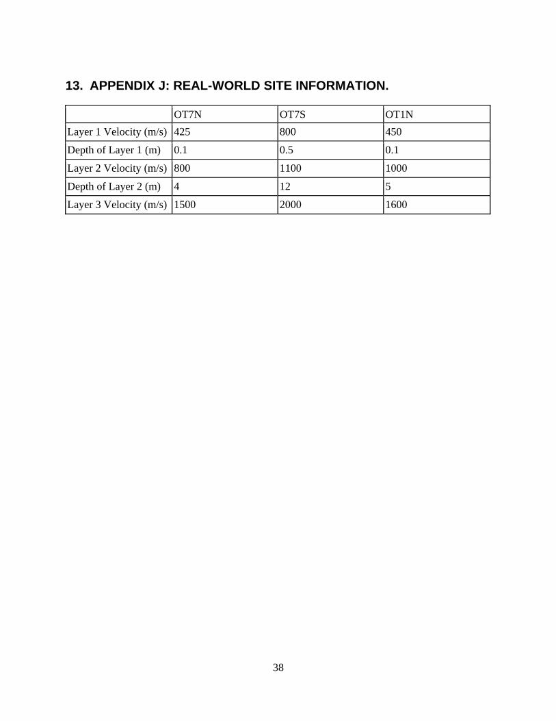
The model being used in this analysis consists of a simulated section of geology that is characterized by a layered near surface geology (currently 2 layers) with a volume fraction consisting of ‘mass’ lumps of varying sizes and densities. In this block is placed a tunnel of specified size, depth, and location. Both the baseline tunnel characteristics and geology are based on real world examples [2] [3]. It is assumed that the location of the tunnel within the model is unknown so a grid search is performed on the surface in an effort to locate the tunnel. Depending on the technology being surveyed, noise is added to the situation to add some level of realism to the problem. The objective is to attempt to detect the tunnel either directly or indirectly using the technologies modeled in this analysis.
1.3.4 Physics Equations
The equations being used consist of a simple set of attenuation equations with the physics of an interface being approximated by sets of expressions for the seismic and EM systems. For the gravity sensor a simple model is used to calculate the gravity at the surface based on the geology directly beneath the sensor. All the calculations are based on scalar physics and do not employ the higher fidelity vector equations that are characteristic of the underlying physics of all the phenomena.
1.4 Independent Variables
The following copy of the input file reflects the current set of independent variables, and the real variables which can be input to the analysis but are not being varied for one reason or another. Input for the algorithms is in an XML format. Variables marked as ‘REAL’ are parameters that are set for all the experiments, those marked as ‘TaguchiVar’ are the variables being varied by the Taguchi methodology.
<Variable type="REAL"> tunnelAlpha 0.32 </Variable > <Variable type="TaguchiVar"> ambientNoise 4 4 4.0e3 19.0e3 </Variable > <Variable type="TaguchiVar"> density_U 5 4 1.61 2.76 </Variable > <Variable type="TaguchiVar"> alpha_U 6 4 0.80 1.1 </Variable > <Variable type="TaguchiVar"> density_L 7 4 1.25 1.65 </Variable > <Variable type="TaguchiVar"> alpha_L 8 4 1.50 2.0 </Variable > <Variable type="TaguchiVar"> seismic_frequency 9 4 10.0 220.0 </Variable > <Variable type="TaguchiVar"> Quality 10 4 2.0 52.0 </Variable > <Variable type="TaguchiVar"> active_Power 11 4 6.0e4 1.0e5 </Variable > <Variable type="TaguchiVar"> passive_Power 12 4 3.0e4 5.0e4 </Variable > <Variable type="TaguchiVar"> Active_detection 13 4 4.0 16.0 </Variable > <Variable type="TaguchiVar"> Passive_detection 14 4 3.0 9.0 </Variable > <Variable type="TaguchiVar"> volumeFraction 15 4 0.01 0.11 </Variable > <Variable type="REAL"> densityDist 2.5 </Variable > <Variable type="REAL"> sizeDist 5.0 </Variable > <Variable type="REAL"> detectionThreshold 2.0 </Variable > <Variable type="TaguchiVar"> EM_SN_detect 16 4 .0 19.0 </Variable > <Variable type="TaguchiVar"> EMNoise 17 4 -14.0 -10 </Variable > <Variable type="TaguchiVar"> tunnelCurrent 18 4 0.1 0.5 </Variable > <Variable type="TaguchiVar"> EM_frequency 19 4 50.0 350.0 </Variable > <Variable type="TaguchiVar"> attenuation_alpha 20 4 0.4 1.0 </Variable > <Variable type="TaguchiVar"> dielectricPermitivity_U 21 4 1.0 16.0 </Variable > <Variable type="REAL"> dielectricPermitivity_L 6.0 </Variable > <Variable type="REAL"> magneticPermeability_U 1.0 </Variable > <Variable type="REAL"> magneticPermeability_L 1.0 </Variable > <Variable type="REAL"> electricalConductivity_L 1.0 </Variable > <Variable type="REAL"> electricalConductivity_U 1.0 </Variable > <Variable type="REAL"> susceptibility_mu_U 1.0 </Variable > <Variable type="REAL"> susceptibility_mu_L 1.0 </Variable > </Parameters> </Analysis> The Taguchi variable information in the above example consists of the variable name used in the models, the column of the orthogonal array that the variable is assigned to, the number of levels for the variable, and the minimum and maximum values that the variable can be assigned. 1.5 Statistical / Noise Variables
The noise variables in a typical run are those identified in the next block. They relate to the mass lumps considered in the gravity sensor calculations.
The random variables cconsist of a name, the mean value, and a standard deviation that is used in the random setting of the variables. The XML parameter ”Statistical_runs” defines the number of repeats for each experiment in which the statistical parameters are varied using a Gaussian distribution.
13
1.6 Taguchi Analysis
The objective of the Taguchi analysis is to determine the mean performance over the range of variables and then examine in detail the impact on performance of each of the independent variables. The experimental structure of this example is based on an L64 orthogonal array which permits us to examine a total of 21 variables in a total of 64 experiments each at 4 experimental levels. The remaining 22 variables were treated as static or random variables. Each experiment was repeated 50 times in which the random variables were reset to capture the uncertainty associated with those random variables.
14
2. TAGUCHI ANALYSIS RESULTS
The raw data generated from the series of experiments is provided in appendix A. The data captures the relative performance of two direct and two indirect tunnel detection technologies. The technologies consisted of active seismic, gravimetric, passive electromagnetic, and passive seismic. The models used in the analysis are provided in the appendices following these sections. In the following figures we present the results of the calculations which demonstrate the impact of the independent variables on the performance of the four systems. The first figure presents the ‘potential’ results of an active seismic system. The term potential is being used because the results represent a theoretical limit, with perfect coupling between the media and the sensor systems. Any engineering solution would operate at levels less than those reported due to engineering limitations.
The vertical axis is the calculated detection performance, or confidence level, per each numbered factor affecting performance on the horizontal axis. A maximum detection performance of 1.0 represents a perfect (100% confidence) detection, while a minimum performance of 0.0 represents a complete failure to detect. The blue diamonds represent the average detection performance of the system over the range of all the variables and their extent. The other diamonds for each level (Level 1, Level 2, Level 3, Level 4) represent the performance at a given variation or perturbation of the factor affecting performance. The higher numerical value for level represents a greater amount of variation; Level 1 is the smallest amount of varation while Level 4 is the largest amount. Each column of diamonds represents the performance of the sensor over the range of the factor or variable identified by the integer below it. In this example, for factor 1 the detection performance varies from approximately 0.1 to 0.3. Factor 1 in this case captures variations in the width of the tunnel on an average over all the remaining independent variables.
Figure 2: Detection vs. factors affecting performance for an active seismic sensor.
15
Using this type of graph we can quickly identify the factors that impact detection performance the most based on the variation in detection performance as each factor is varied. For the active seismic system, factors 3, 8, and 13 seem to be the most significant based on the variation of these independent variables in the analyses. Factor 3 is the depth of the tunnel, factor 8 is the seismic velocity of the lower layer and 13 captures the detection threshold needed to detect the tunnel. This threshold is based on a signal to noise ratio in dBs. Factors 2, the tunnel height, 4, the ambient seismic noise, and 5 the density of the upper layer are close seconds.
In the case of the gravimetric detection methodology, the tunnel depth, factor 3 drives the performance. The tunnel geometry and the material properties of the overburden also impact performance. Caution is advised interpreting the results of the other factors because they represent different physics and in this case capture some nonlinear effects to performance. This confounding effect is a caution that must be exercised with the use of Taguchi techniques. However, it is clear that for this sensor the depth is the dominant factor and that if the tunnel is too deep then the gravimetric sensor is not useful. Specific quantitative conclusions about the useful range of depths cannot be inferred without more engineering details on a specific implementation of this sensor type.
Figure 3: Detection vs. factors affecting performance for a gravimetric sensor.
16
For the passive seismic system, the first 5 factors appear to be the dominant drivers of performance. The first 3 represent the tunnel characteristics, while 4 is the ambient seismic noise and 5 is again the upper layer density. Of course there is also a dependence on the characteristics of the specific seismic sources assumed (Appendix C).
Figure 4: Detection vs. factors affecting performance for a passive seismic sensor.
17
In the case of the electromagnetic system, factors 1, 16, 17, and possibly 20 capture the most performance variation. These factors represent tunnel geometry, the detection capability EM noise and the attenuation of the signal through the layers above the tunnel. The dependence on tunnel geometry is related to the fact that the length of the conductor (wire) is tied to the length of the tunnel, assuming that lights are used for the entire tunnel.
The results for the passive EM sensor have the highest average detection performance out of all of the sensors. However it is clear that this result is directly related to the assumed ambient EM noise, which was based on measured B-field data from a rural environment (Appendix F). Unfortunately noise data from an urban environment were not available for this study. Assumptions were made about the relative increase in noise expected for an urban environment and were employed for the simulations. This introduces a note of caution in immediately concluding that the passive EM sensor is clearly superior to the rest.
The results from the Taguchi analysis of the detection performance for all of the sensors point to the specific factors that have an effect across the board:
Tunnel characteristics: tunnel size and depth
Soil characteristics: the propagation effects of the overburden, including effects of multiple layers with different geologies
Ambient seismic or EM noise
The better a priori data there is for these factors the better we can predict the relative performance of the sensors, and then determine what sensors should be used. It is probably not practical to expect advance information on the tunnel characteristics, although a general profile can be constructed from existing data. However, it is possible to determine some of the soil characteristics and ambient noise in advance of deploying sensors to the field. Based on the
Figure 5: Detection vs. factors affecting performance for a passive EM sensor.
18
results it appears that characterizing the ambient noise is the most important since it has the greatest impact on detection performance.
19
3. CONCLUSION Of the four sensor technologies examined in this study, the most effective based on the Taguchi analysis is passive EM. However this result is undoubtedly influenced by the use of a noise model based on rural data rather than the higher level of noise for an urban environment. This highlights the finding that the ambient noise level is critical in determining which combination of sensors is optimal to use. This is not unexpected, as it is consistent with findings from sensor fusion systems where the sensor with the least ambient noise affecting it will typically have the greatest impact on the result. If ambient seismic noise is relatively low then active or passive seismic sensors are more effective, while if ambient EM noise is relatively low then passive EM (and probably active) sensors are more effective. This suggests a course of action where ambient noise at a given site should be measured prior to making decisions about what kind of sensor suite should be deployed. Additionally, characterizing the geology in advance at a site can help with determining which sensors to deploy. Finally, an estimate of probable tunnel characteristics, especially depth, can aid in estimating the possible performance of sensors. This study has also resulted in a powerful tool based on Taguchi analysis that can be used to evaluate the performance of different sensor suites for a range of scenarios of varying factors that affect detection performance. This tool uses the fundamental physics associated with each sensor rather than previously gathered data. While it presently calculates relative performance of the different sensors, it can be refined to generate absolute detection results as the data used is improved. For example, the more that is known about a specific engineering implementation of a sensor the more accurate the detection result becomes in an absolute sense. Increased quantitative knowledge about ambient noise and geological properties will also improve performance.
20
4. APPENDIX A: RESULTS OF FOUR TUNNEL DETECTION TECHNOLOGIES. MOP 0 (Active seismic) post processed data. Ave= 0.234 0.25 0.312 0.25 0.125 Min - Max: 0.125 - 0.312 0.312 0.125 0.125 0.375 Min - Max: 0.125 - 0.375 0.375 0.438 0.125 0.00 Min - Max: 0.00 - 0.438 0.375 0.25 0.188 0.125 Min - Max: 0.125 - 0.375 0.375 0.125 0.25 0.188 Min - Max: 0.125 - 0.375 0.312 0.188 0.25 0.188 Min - Max: 0.188 - 0.312 0.25 0.25 0.25 0.188 Min - Max: 0.188 - 0.25 0.438 0.25 0.125 0.125 Min - Max: 0.125 - 0.438 0.188 0.25 0.312 0.188 Min - Max: 0.188 - 0.312 0.125 0.25 0.312 0.25 Min - Max: 0.125 - 0.312 0.062 0.312 0.312 0.25 Min - Max: 0.062 - 0.312 0.25 0.312 0.188 0.188 Min - Max: 0.188 - 0.312 0.50 0.312 0.125 0.00 Min - Max: 0.00 - 0.50 0.312 0.188 0.25 0.188 Min - Max: 0.188 - 0.312 0.25 0.25 0.25 0.188 Min - Max: 0.188 - 0.25 0.188 0.25 0.375 0.125 Min - Max: 0.125 - 0.375 0.188 0.25 0.312 0.188 Min - Max: 0.188 - 0.312 0.125 0.25 0.312 0.25 Min - Max: 0.125 - 0.312 0.312 0.062 0.312 0.25 Min - Max: 0.062 - 0.312 0.25 0.312 0.188 0.188 Min - Max: 0.188 - 0.312 0.25 0.312 0.125 0.25 Min - Max: 0.125 - 0.312 MOP 1 (Passive EM) post processed data. Ave= 0.875 0.812 0.75 1.00 0.938 Min - Max: 0.75 - 1.00 0.938 0.875 0.812 0.875 Min - Max: 0.812 - 0.938 1.00 0.875 0.812 0.812 Min - Max: 0.812 - 1.00 0.812 0.875 0.875 0.938 Min - Max: 0.812 - 0.938 0.938 0.812 0.938 0.812 Min - Max: 0.812 - 0.938 0.875 0.875 0.875 0.875 Min - Max: 0.875 - 0.875 0.812 0.875 0.875 0.938 Min - Max: 0.812 - 0.938 0.875 0.875 0.812 0.938 Min - Max: 0.812 - 0.938 0.875 0.812 0.875 0.938 Min - Max: 0.812 - 0.938 0.812 0.875 0.812 1.00 Min - Max: 0.812 - 1.00 0.875 0.75 0.938 0.938 Min - Max: 0.75 - 0.938 0.875 0.938 0.812 0.875 Min - Max: 0.812 - 0.938 0.875 0.875 0.875 0.875 Min - Max: 0.875 - 0.875 0.812 0.875 1.00 0.812 Min - Max: 0.812 - 1.00 0.938 0.812 0.938 0.812 Min - Max: 0.812 - 0.938 0.938 1.00 0.812 0.75 Min - Max: 0.75 - 1.00 1.00 1.00 0.938 0.562 Min - Max: 0.562 - 1.00 0.812 0.938 0.875 0.875 Min - Max: 0.812 - 0.938 0.938 0.875 0.812 0.875 Min - Max: 0.812 - 0.938 0.875 0.75 0.875 1.00 Min - Max: 0.75 - 1.00 0.812 0.875 0.875 0.938 Min - Max: 0.812 - 0.938 MOP 2 (Passive seismic) post processed data. Ave= 0.219 0.375 0.125 0.312 0.062 Min - Max: 0.062 - 0.375 0.25 0.125 0.062 0.438 Min - Max: 0.062 - 0.438 0.375 0.375 0.125 0.00 Min - Max: 0.00 - 0.375 0.50 0.312 0.062 0.00 Min - Max: 0.00 - 0.50 0.375 0.188 0.25 0.062 Min - Max: 0.062 - 0.375
21
0.188 0.25 0.188 0.25 Min - Max: 0.188 - 0.25 0.188 0.25 0.25 0.188 Min - Max: 0.188 - 0.25 0.25 0.125 0.25 0.25 Min - Max: 0.125 - 0.25 0.125 0.125 0.312 0.312 Min - Max: 0.125 - 0.312 0.125 0.188 0.312 0.25 Min - Max: 0.125 - 0.312 0.125 0.188 0.25 0.312 Min - Max: 0.125 - 0.312 0.188 0.188 0.25 0.25 Min - Max: 0.188 - 0.25 0.312 0.188 0.188 0.188 Min - Max: 0.188 - 0.312 0.375 0.25 0.125 0.125 Min - Max: 0.125 - 0.375 0.25 0.25 0.188 0.188 Min - Max: 0.188 - 0.25 0.188 0.25 0.188 0.25 Min - Max: 0.188 - 0.25 0.188 0.25 0.25 0.188 Min - Max: 0.188 - 0.25 0.188 0.188 0.25 0.25 Min - Max: 0.188 - 0.25 0.312 0.188 0.188 0.188 Min - Max: 0.188 - 0.312 0.25 0.312 0.188 0.125 Min - Max: 0.125 - 0.312 0.25 0.312 0.125 0.188 Min - Max: 0.125 - 0.312 MOP 3 (Gravimetric) post processed data. Ave= 0.284 0.25 0.305 0.209 0.371 Min - Max: 0.209 - 0.371 0.25 0.242 0.33 0.312 Min - Max: 0.242 - 0.33 0.951 0.121 0.062 0.00 Min - Max: 0.00 - 0.951 0.25 0.271 0.25 0.364 Min - Max: 0.25 - 0.364 0.434 0.25 0.242 0.209 Min - Max: 0.209 - 0.434 0.309 0.305 0.279 0.242 Min - Max: 0.242 - 0.309 0.212 0.239 0.309 0.375 Min - Max: 0.212 - 0.375 0.364 0.279 0.246 0.246 Min - Max: 0.246 - 0.364 0.25 0.312 0.301 0.271 Min - Max: 0.25 - 0.312 0.212 0.301 0.312 0.309 Min - Max: 0.212 - 0.312 0.368 0.309 0.216 0.242 Min - Max: 0.216 - 0.368 0.25 0.25 0.298 0.338 Min - Max: 0.25 - 0.338 0.305 0.275 0.309 0.246 Min - Max: 0.246 - 0.309 0.242 0.216 0.305 0.371 Min - Max: 0.216 - 0.371 0.312 0.309 0.301 0.212 Min - Max: 0.212 - 0.312 0.246 0.309 0.279 0.301 Min - Max: 0.246 - 0.309 0.334 0.301 0.25 0.25 Min - Max: 0.25 - 0.334 0.371 0.312 0.239 0.212 Min - Max: 0.212 - 0.371 0.242 0.279 0.309 0.305 Min - Max: 0.242 - 0.309 0.275 0.298 0.312 0.25 Min - Max: 0.25 - 0.312 0.246 0.246 0.275 0.368 Min - Max: 0.246 - 0.368
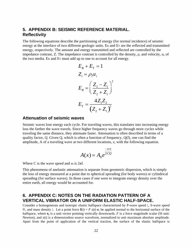
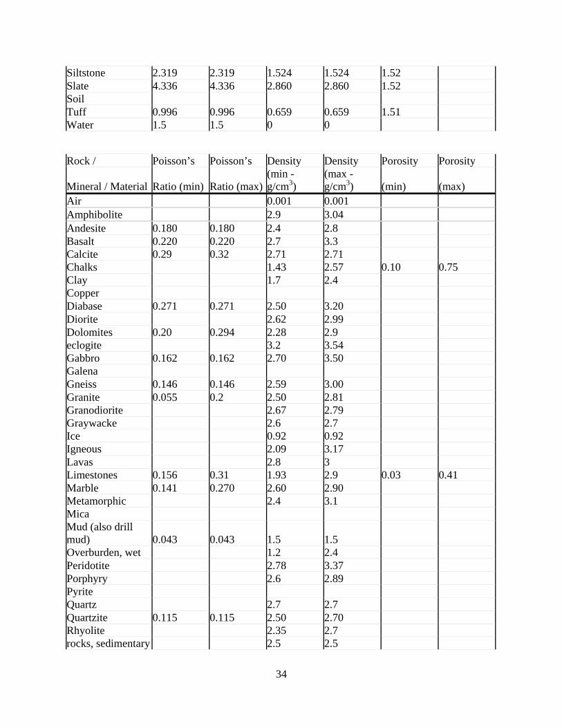
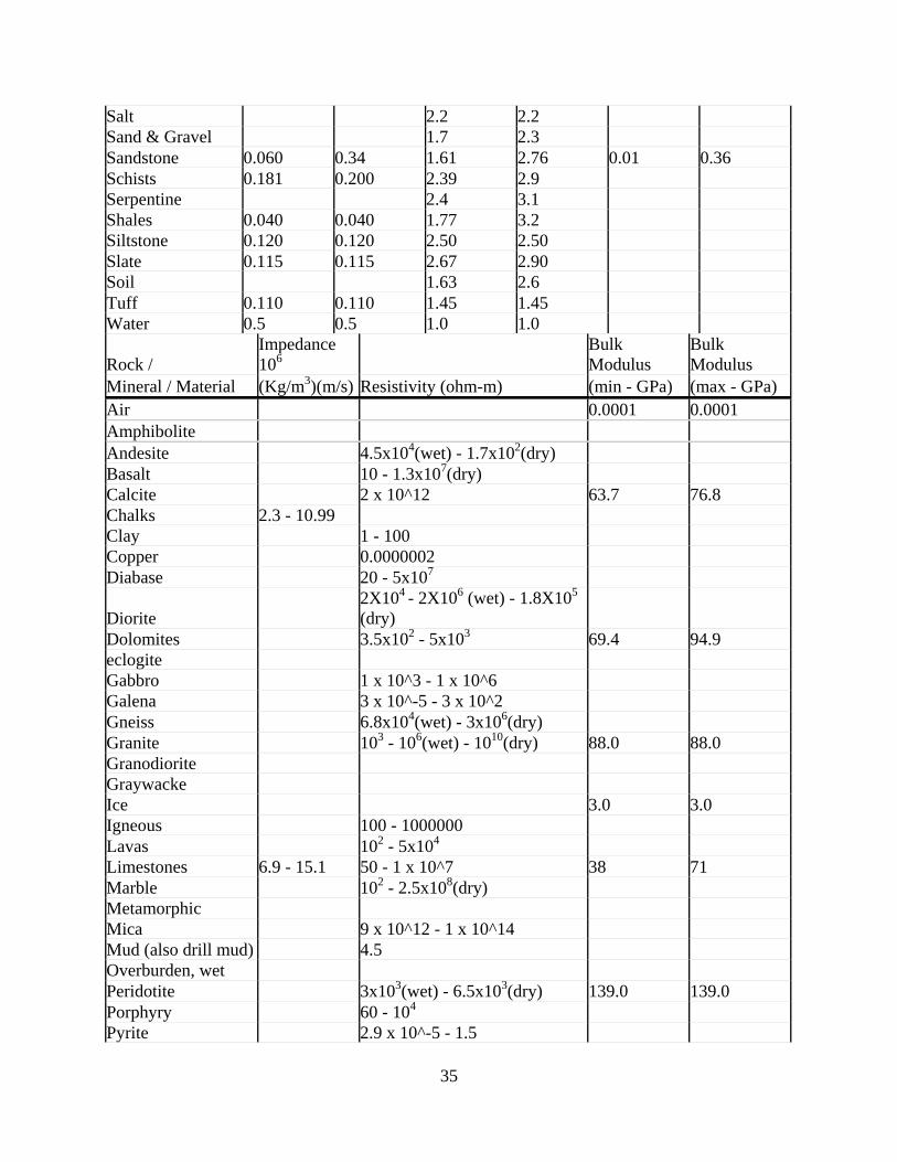
The following equations describe the partitioning of energy (for normal incidence) of seismic energy at the interface of two different geologic units. ER and ET are the reflected and transmitted energy, respectively. The amount and energy transmitted and reflected are controlled by the impedance contrast, Z. The impedance contrast is controlled by the density, ρ, and velocity, α, of the two media. ER and ET must add up to one to account for all energy.
Attenuation of seismic waves
Seismic waves lose energy each cycle. For traveling waves, this translates into increasing energy loss the farther the wave travels. Since higher frequency waves go through more cycles while traveling the same distance, they attenuate faster. Attenuation is often described in terms of a quality factor, Q. Given Q, which is often a function of frequency, Q(f), one can find the amplitude, A of a traveling wave at two different locations, x, with the following equation.
Where C is the wave speed and ω is 2πf.
This phenomena of anelastic attenuation is separate from geometric dispersion, which is simply the loss of energy measured at a point due to spherical spreading (for body waves) or cylindrical spreading (for surface waves). In those cases if one were to integrate energy density over the entire earth, all energy would be accounted for.
6. APPENDIX C: NOTES ON THE RADIATION PATTERN OF A VERTICAL VIBRATOR ON A UNIFORM ELASTIC HALF-SPACE. Consider a homogeneous and isotropic elastic halfspace characterized by P-wave speed , S-wave speed , and mass density . Let a point force f(t) = F s(t) ez be applied normal to the horizontal surface of the halfspace, where ez is a unit vector pointing vertically downwards. F is a force magnitude scalar (SI unit: Newton), and s(t) is a dimensionless source waveform, normalized to unit maximum absolute amplitude. Apart from the point of application of the vertical traction, the surface of the elastic halfspace is
ER ET 1
Zi i i
ER Z2 Z1
Z2 Z1
2
ET 4Z1Z2
Z2 Z1 2
A(x) A0e x
2CQ
23
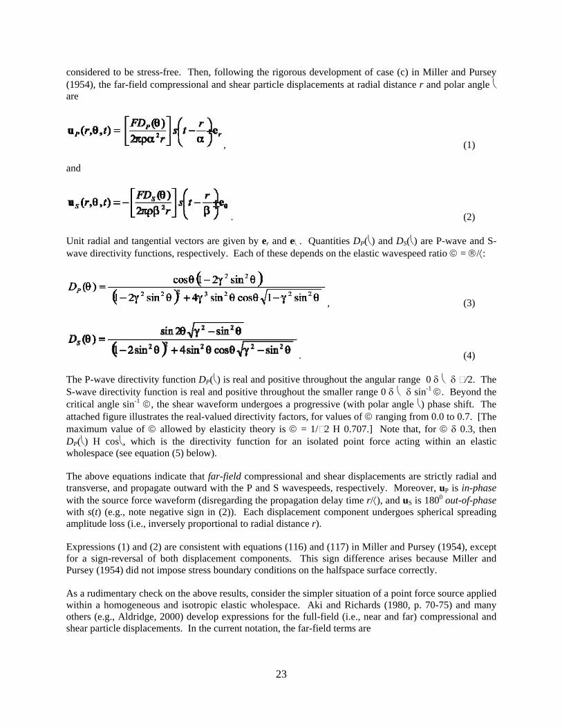
considered to be stress-free. Then, following the rigorous development of case (c) in Miller and Pursey (1954), the far-field compressional and shear particle displacements at radial distance r and polar angle are
, (1) and
. (2) Unit radial and tangential vectors are given by er and e . Quantities DP() and DS() are P-wave and S-wave directivity functions, respectively. Each of these depends on the elastic wavespeed ratio = /:
, (3)
. (4)
The P-wave directivity function DP() is real and positive throughout the angular range 0 /2. The S-wave directivity function is real and positive throughout the smaller range 0 sin-1 . Beyond the critical angle sin-1 , the shear waveform undergoes a progressive (with polar angle ) phase shift. The attached figure illustrates the real-valued directivity factors, for values of ranging from 0.0 to 0.7. [The maximum value of allowed by elasticity theory is = 1/ 2 0.707.] Note that, for 0.3, then DP() cos, which is the directivity function for an isolated point force acting within an elastic wholespace (see equation (5) below). The above equations indicate that far-field compressional and shear displacements are strictly radial and transverse, and propagate outward with the P and S wavespeeds, respectively. Moreover, uP is in-phase with the source force waveform (disregarding the propagation delay time r/), and uS is 1800 out-of-phase with s(t) (e.g., note negative sign in (2)). Each displacement component undergoes spherical spreading amplitude loss (i.e., inversely proportional to radial distance r). Expressions (1) and (2) are consistent with equations (116) and (117) in Miller and Pursey (1954), except for a sign-reversal of both displacement components. This sign difference arises because Miller and Pursey (1954) did not impose stress boundary conditions on the halfspace surface correctly. As a rudimentary check on the above results, consider the simpler situation of a point force source applied within a homogeneous and isotropic elastic wholespace. Aki and Richards (1980, p. 70-75) and many others (e.g., Aldridge, 2000) develop expressions for the full-field (i.e., near and far) compressional and shear particle displacements. In the current notation, the far-field terms are
24
, (5) and
. (6) Note that the wholespace formulae are similar in structure to the corresponding halfspace formulae. The directivity functions are replaced by ordinary trigonometric functions, and the numerical divisor is 4 instead of 2 . Obviously, both directivity functions are well-defined (i.e., real-valued) throughout the full angular range 0 (although the P-wave directivity cos changes sign at polar angle = /2). Far-field compressional and shear displacements are again strictly radial and transverse, respectively, and propagate with P and S wavespeeds. Amplitude loss is spherical. Finally, comparison of the halfspace and wholespace expressions indicates that the phase relationships of far-field displacements with respect to the source force waveform are preserved (at least within the common angular range of both directivity functions). References Aki, K., and Richards, P.G., 1980, Quantitative seismology, theory and methods, volume I: W.H.
Freeman and Company. Aldridge, D.F., 2000, Radiation of elastic waves from point sources in a uniform wholespace: Sandia
National Laboratories Technical Report SAND2000-1767. Miller, G.F., and Pursey, H., 1954, The field and radiation impedance of mechanical radiators on the free
surface of a semi-infinite isotropic solid: Proceedings of the Royal Society, Series A, 223, 521-541. David F. Aldridge Geophysics Department Sandia National Laboratories Albuquerque, New Mexico, USA, 87185-0750 10 February 2006
25
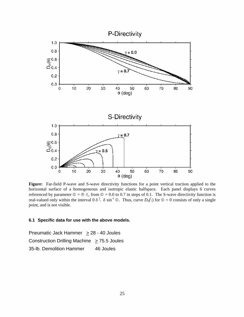
Figure: Far-field P-wave and S-wave directivity functions for a point vertical traction applied to the horizontal surface of a homogeneous and isotropic elastic halfspace. Each panel displays 6 curves referenced by parameter = /, from = 0.0 to 0.7 in steps of 0.1. The S-wave directivity function is real-valued only within the interval 0 sin-1 . Thus, curve DS() for = 0 consists of only a single point, and is not visible. 6.1 Specific data for use with the above models.
Pneumatic Jack Hammer > 28 - 40 Joules
Construction Drilling Machine > 75.5 Joules
35-lb. Demolition Hammer 46 Joules
26
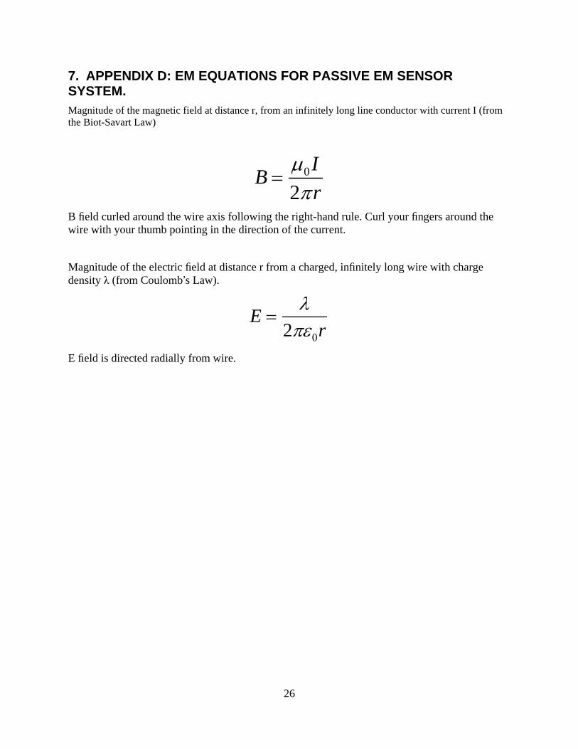
7. APPENDIX D: EM EQUATIONS FOR PASSIVE EM SENSOR SYSTEM. Magnitude of the magnetic field at distance r, from an infinitely long line conductor with current I (from the Biot-Savart Law)
B field curled around the wire axis following the right-hand rule. Curl your fingers around the wire with your thumb pointing in the direction of the current.
Magnitude of the electric field at distance r from a charged, infinitely long wire with charge density λ (from Coulomb’s Law).
E field is directed radially from wire.
B 0I
2r
E
20r
27
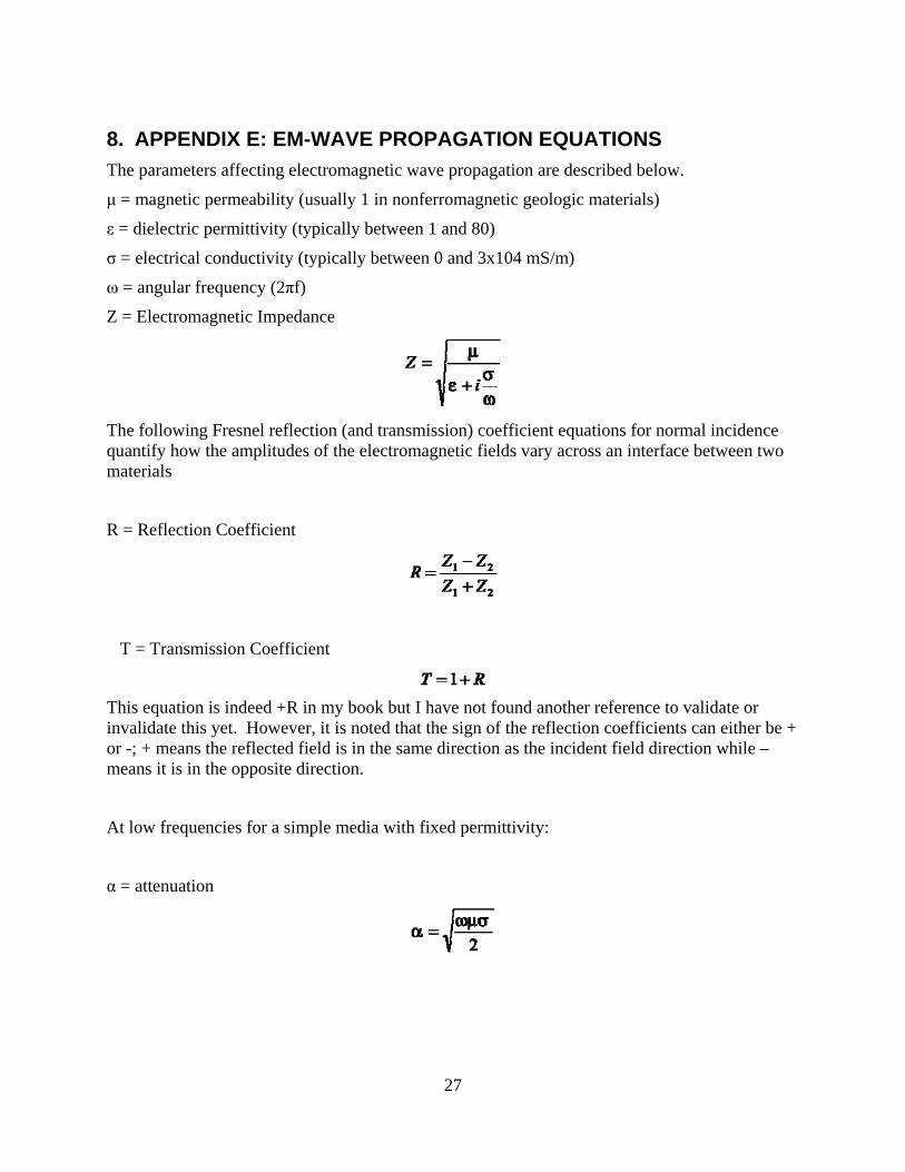
8. APPENDIX E: EM-WAVE PROPAGATION EQUATIONS
The parameters affecting electromagnetic wave propagation are described below.
μ = magnetic permeability (usually 1 in nonferromagnetic geologic materials)
ε = dielectric permittivity (typically between 1 and 80)
σ = electrical conductivity (typically between 0 and 3x10⁴ mS/m)
ω = angular frequency (2πf)
Z = Electromagnetic Impedance
The following Fresnel reflection (and transmission) coefficient equations for normal incidence quantify how the amplitudes of the electromagnetic fields vary across an interface between two materials
R = Reflection Coefficient
T = Transmission Coefficient
This equation is indeed +R in my book but I have not found another reference to validate or invalidate this yet. However, it is noted that the sign of the reflection coefficients can either be + or -; + means the reflected field is in the same direction as the incident field direction while – means it is in the opposite direction.
At low frequencies for a simple media with fixed permittivity:
α = attenuation
28
9. APPENDIX F: B-FIELD EM NOISE
29
10. APPENDIX G: GRAVIMETRIC INFORMATION. Theory of Gravity
Use two of Newtons laws:
1) Universal law of gravitation:
2) Second law of motion:
we combine these expressions to obtain the gravitational acceleration at the surface of the earth:
Note: g is a vector field with the gravitational potential defined as:
U is a scalar field which simplifies use.
Definition: The gravitational potential, U, due to a point mass m, at a distance r from m, is the work done by the gravitational force in moving a unit mass from infinity to to a position r from m.
Relating g to U.
U is a scalar field which makes it easier to work with:
• Potentials are additive
• Gravity is a conservative force
• And gravitational acceleration can be easily determined from the potential…
Given:
It follows that:
For smaller scale problems we usually deal with g, and sum the vertical component of g…
Gravity anomalies.
Sum contributions in the vertical direction.
F Gm1m2
r2
F mg
g GM E
RE2
U Gm
r
U Gm
r
g U
r
Gm
r2
Figure
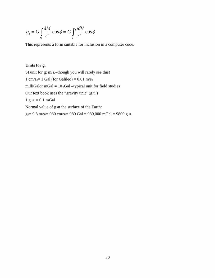
gz
30
This represents a form suitable for inclusion in a computer code.
Units for g.
SI unit for g: m/s2–though you will rarely see this!
1 cm/s2= 1 Gal (for Galileo) = 0.01 m/s2
milliGalor mGal = 10-3Gal –typical unit for field studies
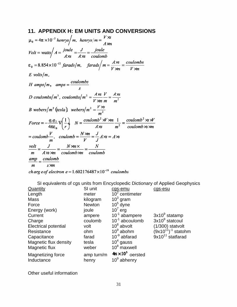
SI equivalents of cgs units from Encyclopedic Dictionary of Applied Geophysics
Quantity SI unit cgs-emu cgs-esu Length meter 102 centimeter Mass kilogram 103 gram Force Newton 105 dyne Energy (work) joule 107 erg Current ampere 10-1 abampere 3x10⁹ statamp Charge coulomb 10-1 abcoulomb 3x10⁹ statcoul Electrical potential volt 108 abvolt (1/300) statvolt Resistance ohm 109 abohm (9x10¹¹)-1 statohm Capacitance farad 10-9 abfarad 9x10¹¹ statfarad Magnetic flux density tesla 104 gauss Magnetic flux weber 108 maxwell
Magnetizing force amp turn/m oersted Inductance henry 109 abhenry
Other useful information
32
B (magnetic induction or magnetic flux density) is in units of tesla, H (magnetic field) is in units of amp turns/m, E (electric field) is in units of volts/m.
r = relative dielectric permittivity, = electrical conductivity, V = velocity, = attenuation.
40
Note: measured at 100MHz
41
15. REFERENCES
[1] Madhan S. Phadke, Quality Engineering Using Robust Design, PTR Prentice Hall, Upper Saddle River, NJ, 1995.
[2] Troy R. Brosten, Robert F. Ballard, Jr. and Lillian D. Wakeley, Cave and Tunnel Detection, a State-of-the-Art Assessment, US Army Corps of Engineers Engineer Research and Development Center, April 2003.
[3] Jason R. McKenna, Robert Horton, Gregory Elbring, Amy Clymer and Clifford Hansen, Tunnel Detection Technology Demonstrations: Otay Mesa and Calexico, California, US Army Corps of Engineers Engineer Research and Development Center, December 2006.
42
16. DISTRIBUTION 2 MS1161 Mike Senglaub 5432 2 MS1161 Mark Yee 5432 2 MS1161 K. Terry Stalker 5432 1 MS1161 Dan Rondeau 5430 1 MS0769 Ron Moya 6400 1 MS0757 J.R. Russell 6414 1 MS0750 Greg Elbring 6734 1 MS0750 Rob Abbott 6734 1 MS0750 Nedra Bonal 6734 1 MS0484 Russ Skocypec 8004 1 MS9151 James Costa 8950 1 MS0899 Technical Library 9536 (electronic copy) 1 MS0123 D. Chavez, LDRD Office 1011