Page 1
SENSOR MODELING AND
LINEARIZATION USING ARTIFICIAL
NEURAL NETWORK TECHNIQUE
A Thesis submitted in partial fulfillment of the requirements for the degree of
Master of Technology
in
Electronics and Communication Engineering
Specialization: Electronics and Instrumentation Engineering
by
SUNIL RATHOD
Roll No.: 213EC3227
Department of Electronics and Communication Engineering
National Institute of Technology, Rourkela
Odisha- 769008, India
May 2015
Page 2
SENSOR MODELING AND
LINEARIZATION USING ARTIFICIAL
NEURAL NETWORK TECHNIQUE
A Thesis submitted in partial fulfillment of the requirements for the degree of
Master of Technology
in
Electronics and Communication Engineering
Specialization: Electronics and Instrumentation Engineering
by
SUNIL RATHOD
Roll No.: 213EC3227
Under the Supervision of
Prof. KAMALAKANTA MAHAPATRA
Department of Electronics and Communication Engineering
National Institute of Technology, Rourkela
Odisha- 769008, India
May 2015
Page 3
Dept. of Electronics and Communication Engineering
National Institute of Technology, Rourkela
Odisha- 769008, India
CERTIFICATE
This is to certify that the work in the thesis entitled “SENSOR MODELING AND
LINEARIZATION USING ARTIFICIAL NEURAL NETWORK
TECHNIQUE” by Mr. SUNIL RATHOD, Roll No. 213EC3227 is a record of an
original and authentic research work carried out by him during the session 2014 –
2015 under my supervision and guidance in partial fulfillment of the requirements
for the award of the degree of Master of Technology in Electronics and
Communication Engineering (Electronics and Instrumentation), National Institute of
Technology, Rourkela.
To the best of my knowledge, the work in this thesis has not been submitted to any
other University / Institute for the award of any degree or diploma.
______________________________
Prof. Kamalakanta Mahapatra
Date: Dept. of Electronics and Communication Engg.
Place: Rourkela National Institute of Technology, Rourkela
Page 4
DEDICATED TO
MY TEACHERS,
FRIENDS &
MY PARENTS
Page 5
i
ACKNOWLEDGEMENTS
I would like to express my deep sense of respect and gratitude towards my supervisor
and guide Prof. Kamalakanta Mahapatra who has been a guiding force behind
this work. I am highly obliged and grateful for his excellent guidance, endless
encouragement and cooperation extended to me right from the onset of this task till
its successful completion. I consider myself fortunate to work under such a
wonderful person.
I am very thankful to Prof. T.K. Dan and Prof. U.C. Pati for their valuable
suggestions during the reviews of this work. I am also thankful to Prof. A.K. Swain,
Prof. D.P. Acharya and Prof. S.K. Patra for teaching me and helping me in every
aspect throughout my M.Tech. Course duration.
My sincere thanks to PhD Sir Mr. Subhransu Padhee for his encouragements,
suggestions and feedbacks which have always motivated me. I would like to thank
my friends and classmates, in particular, for the fun and enjoyment that we have
shared for the last two years of my stay in NIT Rourkela. The stay at NIT Rourkela
would not have been so wonderful without them.
I am indebted to my parents for their love, affection and sacrifice. Their
unconditional support and encouragement has always been a guiding force.
SUNIL RATHOD
Page 6
ii
ABSTRACT
Many Sensors show a nonlinear relationship between their input and output. Sometimes the reason
for nonlinearity is inherent and sometimes it is due to the changes in the environmental parameters
like temperature and humidity. Ageing is also responsible for the nonlinearity of sensors. Due to
the presence of nonlinearity, it becomes very difficult to directly read the sensor over its whole
sensing range. The accuracy of the device is affected if it is used in its full input range. Hence it is
very much necessary to study the problem of nonlinearity present in sensors and to solve it.
Thermistor and thermocouple are the temperature sensors that exhibit nonlinear characteristics.
Thermistor is the most nonlinear device but thermocouple is linear if operated in a specific
operating temperatures. Thermocouple shows nonlinearity if operated in its entire operating range.
The nonlinearity of a sensor can be compensated by designing an inverse model of the sensor and
connecting it in series with the sensor. This enables the digital readout of the output of the sensor.
So the inverse models of these temperature sensors are designed and connected in series with them,
so that the associated nonlinearity can be compensated and the output can be read digitally. The
neural network technique seems to be an ideal technique for designing the inverse model of such
sensors. Also, a direct model of such sensors is also designed which can be used for calibrating
inputs and for fault detection. A technique for linearizing the output of the sensor without using
inverse modeling is also discussed.
Page 7
iii
CONTENTS
ACKNOWLEDGEMENTS ........................................................................................................................ i
ABSTRACT ................................................................................................................................................ ii
CONTENTS ............................................................................................................................................... iii
LIST OF FIGURES .....................................................................................................................................v
1 INTRODUCTION ...............................................................................................................................2
1.1 Static Characteristics of a sensor ...................................................................................................2
1.1.1 Accuracy ....................................................................................................................................2
1.1.2 Precision ....................................................................................................................................2
1.1.3 Error ...........................................................................................................................................3
1.1.4 Correction ..................................................................................................................................3
1.1.5 Uncertainty ................................................................................................................................4
1.1.6 Hysteresis ..................................................................................................................................4
1.1.7 Repeatability ..............................................................................................................................4
1.1.8 Sensitivity ..................................................................................................................................5
1.1.9 Resolution ..................................................................................................................................5
1.1.10 Linearity ....................................................................................................................................6
1.2 Dynamic Characteristics of a sensor .............................................................................................7
1.3 Motivation .....................................................................................................................................7
1.4 Literature Review ..........................................................................................................................8
2 ARTIFICIAL NEURAL NETWORK TECHNIQUE ....................................................................12
2.1 Properties of ANN .......................................................................................................................12
2.1.1 Power .......................................................................................................................................13
2.1.2 Ease of use ...............................................................................................................................13
2.1.3 Nonlinearity .............................................................................................................................13
2.1.4 Adaptivity ................................................................................................................................13
2.1.5 VLSI Implementation ..............................................................................................................13
2.2 Model of a neuron .......................................................................................................................14
2.3 Multilayer Perceptron (MLP) ......................................................................................................17
2.4 Back-propagation Algorithm .......................................................................................................19
2.5 Application of Neural Network ...................................................................................................21
2.5.1 System Identification ...............................................................................................................22
Page 8
iv
2.5.2 Inverse Modeling .....................................................................................................................23
3 DIRECT MODELING AND INVERSE MODELING OF A THERMISTOR ...........................25
3.1 Thermistor ...................................................................................................................................25
3.1.1 Basic Operation .......................................................................................................................25
3.1.2 Thermistor Classification ........................................................................................................25
3.1.3 Thermistor Mathematical Models ...........................................................................................26
3.1.4 Self Heating Effect of thermistor.............................................................................................29
3.2 Voltage Divider Circuit ...............................................................................................................29
3.3 Development of Direct Model and Inverse Model of Thermistor ...............................................30
3.3.1 Direct Modeling .......................................................................................................................30
3.3.2 Inverse Modeling .....................................................................................................................31
3.4 Simulation Results .......................................................................................................................31
3.4.1 Neural network based direct modeling of thermistor ..............................................................32
3.4.2 Neural network based inverse modeling of thermistor ............................................................33
4 DIRECT MODELLING AND INVERSE MODELLING OF A THERMOCOUPLE ..............35
4.1 Thermocouple ..............................................................................................................................35
4.1.1 Principle of operation ..............................................................................................................35
4.1.2 Polynomial Model of thermocouple ........................................................................................36
4.1.3 Thermocouple Measurement ...................................................................................................36
4.1.4 Ageing of thermocouple ..........................................................................................................37
4.1.5 Types of thermocouple ............................................................................................................38
4.2 Development of Direct Model and Inverse Model of Thermocouple .........................................39
4.2.1 Direct Modeling .......................................................................................................................40
4.2.2 Inverse Modeling .....................................................................................................................41
4.3 Simulation Results .......................................................................................................................41
4.3.1 Neural network based direct modeling of thermocouple .........................................................41
4.3.2 Neural network based inverse modeling of thermocouple ......................................................43
5 NEURAL NETWORK BASED SENSOR LINEARIZATION .....................................................45
5.1 Simulation Results .......................................................................................................................46
6 CONCLUSION ..................................................................................................................................48
BIBLIOGRAPHY .....................................................................................................................................49
Page 9
v
LIST OF FIGURES
Fig. 1. 1 : Hysteresis Curve .........................................................................................................................4
Fig. 1. 2 : Nonlinear characteristic of a thermistor ......................................................................................6
Fig. 2. 1 : Model of Neuron ...................................................................................................................... 14
Fig. 2. 2 : Threshold Activation Function ................................................................................................ 15
Fig. 2. 3 : Signum Activation Function .................................................................................................... 16
Fig. 2. 4 : Sigmoid Activation Function ................................................................................................... 16
Fig. 2. 5 : Hyperbolic Tangent Activation Function................................................................................. 17
Fig. 2. 6 : Structure of Multilayer Perceptron........................................................................................... 18
Fig. 2. 7 : Two basic signal flows in a Multilayer Perceptron .................................................................. 19
Fig. 2. 8 : Neural Network employing Back-propagation Algorithm....................................................... 20
Fig. 2. 9 : Block diagram of System Identification .................................................................................. 22
Fig. 2. 10 : Block diagram of Inverse System Modeling ............................................................................ 23
Fig. 3.1 : Characteristic of a thermistor ................................................................................................... 28
Fig. 3. 2 : Voltage Divider Circuit for Resistance to Voltage Conversion of a thermistor ...................... 29
Fig. 3. 3 : A scheme for direct modeling of Thermistor with VDC using neural network based model .. 30
Fig. 3. 4 : A scheme for inverse modeling of Thermistor with VDC using neural network based model 31
Fig. 3.5 : Plot of Actual and Estimated Output of thermistor sensor ....................................................... 32
Fig. 3. 6 : Plots of forward, inverse and overall characteristics of the thermistor .................................... 33
Fig. 4. 1 : Thermocouple measurement scheme ....................................................................................... 37
Fig. 4. 2 : Characteristic functions of different thermocouple types ........................................................ 38
Fig. 4. 3 : A scheme for direct modeling of Thermocouple using neural network based model .............. 40
Fig. 4. 4 : A scheme for inverse modeling of Thermocouple using neural network based model ........... 41
Fig. 4. 5 : Plot of Actual and Estimated Output of thermocouple sensor ................................................. 42
Fig. 4. 6 : Plots of forward, inverse and overall characteristics of the thermocouple .............................. 43
Fig. 5. 1 : Neural Network based Linearization (a) Training and (b) Testing .......................................... 45
Fig. 5. 2 : Characteristics of the sensor before and after linearization suing neural network ................... 46
Page 11
2
1 INTRODUCTION
The devices which convert the physical input quantities into electrical or any different physical
quantity for the purpose of measurement are known as sensors. The Instrument Society of America
has defined the sensor as “a device which provides a usable output in response to a specified
measurand”. Sensors and transducers are the basic devices needed to sense and convert the
physical parameters to a convenient form. The convenient form of the measurement is, most
commonly, an electrical signal, which has many advantages compared to other forms such as
optical, fluidic and mechanical. A sensor is unique while the transducer is composite. A sensor
structure gets more physically attached to the environment under operation than the transducer.
1.1 Static Characteristics of a sensor
Static characteristics are related to the amplitude of the response or the output of the system when
the measurand or input does not vary with time. The important static characteristics are discussed
below.
1.1.1 Accuracy
Accuracy can be defined as the capacity of an instrument system that gives a result that is near to
the true or ideal value. The true or ideal value is the standard against which the system can be
calibrated. The measured value of most systems fails to represent the true value either due to the
effects inherent to the system or other interfering inputs such as temperature, humidity and
vibration. The accuracy of the system given by
𝐴 = 1 − |𝑌 − 𝑋
𝑌| (1.1)
where
𝑋 is the measured value
𝑌 is the true or ideal value
Accuracy is generally expressed in percentage form as
%𝐴 = 𝐴 × 100 (1.2)
1.1.2 Precision
Precision is the characteristics of a measuring system that indicates how closely it repeats the same
value of the outputs when the same inputs are applied to the system under the same operating and
Page 12
3
environmental conditions. Although there is very less likelihood that the output response is exactly
repeated, the closeness of repetition can be considered by taking a cluster of repeating points. The
degree of this precision is expressed as the probability of a large number of readings falling within
the cluster of closeness. However such closeness may not have closeness to the true value. Hence
an accurate system is also precise but a precise system may not be accurate.
Let us take N readings of the measurements of which the mean value is
= 1
𝑁∑ 𝑋𝑛
𝑁𝑛=1 𝑁 = Number of data (1.3)
The precision of measurement is given by
𝑃 = 1 − |𝑋𝑛 −
| (1.4)
1.1.3 Error
The deviation of the output or response of the system from true or ideal value is defined as the
error of the system. The difference of the measured value and the true value is taken to calculate
error. This is called absolute error. Sometimes, the error is calculated as a percentage of the full
scale range or with respect to the span of the instrument. Therefore the error is expressed is
𝜀 = 𝑋 − 𝑌 (1.5)
and
%𝜀 =𝑋 − 𝑌
𝑌𝐹𝑆× 100 (1.6)
where, 𝑌𝐹𝑆 = true or ideal full scale value.
1.1.4 Correction
During the calibration of the instrument, the error has to be compensated using a calibrating
circuit. The correction is the value to be added with the measured value to get the true value.
Hence the correction can be expressed as
Correction = 𝑌 − 𝑋 = −𝜀 (1.7)
Depending on the polarity of deviation from the true value, the correction can be either positive or
negative.
Page 13
4
1.1.5 Uncertainty
Uncertainty is a term similar to error, which is used to express the deviation of the instrument from
the actual value. It is the range of the deviation of the measured value from the true value.
Uncertainty is also alternatively defined as a limiting error and expressed as a percentage of full
scale reading.
1.1.6 Hysteresis
Many sensors with primary sensing devices made of elastic members show a difference between
the two output readings for the same input, depending on the direction of successive input values
either incresing or decreasing, This difference in output values is known as hysteresis. Hysteresis
is a characteristic of not only mechanical or magnetic elements but also of many chemical and
biochemical devices. A ferromegnetic material shows hysteresis effect upon magnetization and
subsequent demagnerization. Many chemical sensors upon being exposed to chemicals get their
sensitivity deformed and show a hysteresis effect.
1.1.7 Repeatability
Repeatability of an instrument signifies the degree of closeness of a set of measurements for the
same input obtained by the same observer with the same method and apparatus under the same
0
1
2
3
4
5
6
7
8
9
10
0 2 4 6 8 10
Outp
ut
Input
Increasing Input
Decreasing Input
Fig. 1. 1 Hysteresis Curve
Page 14
5
operating conditions, but for a short duration of operation. Alternatively, it can be defined as it is
the degree of conformity by which a set of reading is produced again and again for a particular
value of input. It must be noted that the surrounding conditions should be same during the entire
process.
1.1.8 Sensitivity
When a measuring instrument is used to measure an unknown quantity 𝑥, we need to know how
the instrument relates the amplitude of input 𝑥 with the amplitude of output or response 𝑦. This
input-output- relationship is called sensitivity. Quantitatively, the sensitivity at any measuring
point 𝑖 is given by the slope
𝑆𝑖 =𝑑𝑦𝑖
𝑑𝑥𝑖 (1.8)
where 𝑥𝑖 and 𝑦𝑖 are the input and output at the measuring point 𝑖. It is desirable that a sensor has
a constant sensitivity so that
𝑑𝑦𝑖
𝑑𝑥𝑖= 𝐾 for 𝑖 = 1, 2, 3,…, 𝑚 (1.9)
where 𝑚 is the measuring point of the highest operating range.
1.1.9 Resolution
A measuring instrument produces the smallest output quantity on application of smallest input.
The smallest input for which the system produces the detectable output is called its resolution. The
resolution is mostly a characteristic inherent to the measuring system that depends on its geometry
or structural factors.
Page 15
6
1.1.10 Linearity
The measuring instruments possess some undesirable characteristics due to which the actual output
deviates from true or ideal values. The causes of deviation ate various, including the inherent
design characteristics and interfering inputs. Many instruments show a typical deviation from a
trend of outputs even without interfering inputs making the system nonlinear. Such a characteristic
of a measuring system is essential for calibrating the instrument by adopting various linearization
techniques. In fact, when the sensitivity is constant over the operating range, the calibration
characteristic is a straight line either passing through the origin or intercepting any one of the axis.
When the sensitivity changes or does remain constant over the operating range, the instrument is
said to be non-linear. Linearity is a quantity that denotes the maximum the maximum deviation of
the output from the true value as the percentage of the true value. The lesser this value, higher is
the linearity.
0
50000
100000
150000
200000
250000
-40 -20 0 20 40 60 80 100 120 140
Res
ista
nce
in Ω
Temperature in degree Celsius
Fig. 1. 2 Nonlinear characteristic of a thermistor
Page 16
7
1.2 Dynamic Characteristics of a sensor
When the energy storing elements are present in a system then the sensors show dynamic behavior
for a time varying input than a time-invariant input. The dynamic behavior of these systems
depends on their own characteristics as well as the dynamic characteristics of the input signal.
Different types of time varying signals are employed for a measuring system. But the dynamic
characteristics of the measuring system are explained with respect to few common input signals
such as step and ramp signals.
1.3 Motivation
The sensors shows nonlinear relationship between its input and output which limits their dynamic
range. It becomes very difficult to read the output digitally over a whole input range of the sensor.
So it is a challenging task to design and implement sensors which are free from the problem of
nonlinearity associated with them. Also the accuracy in measurement is affected greatly due to
ageing of the sensor and environmental parameters like temperature and humidity.
Thermistor and thermocouple are such sensors that exhibit nonlinear characteristics. The
nonlinearity of a sensor can be compensated by designing an inverse model of the sensor and
connecting it in series with it. This enables the digital readout of the output of the sensor. Also, a
direct model of such sensors can be designed for the purpose calibrating inputs and for fault
detection. Apart from developing an inverse model, a sensor can be linearized directly using neural
networks.
So, the problems associated with the nonlinearity of the sensors along with the variations in
nonlinearity with environmental changes motivated in the areas of modeling and linearization of
the sensors.
Page 17
8
1.4 Literature Review
I. D. Patranabis, S. Ghosh, C. Bakshi; “Linearizing Transducer Characteristics”.
In this paper [1], the practical transducers are categorized into two types according to the
relationship between their inputs and outputs. Type I is the one whose characteristics is
exponentially rising whereas Type II is having characteristic that is exponentially decaying.
Transducers with Type I characteristics can be easily linearized using logarithmic converters but
Type II requires additional inverting ways so that it can be linearized. Although advantages of
digital linearizing methods are given, the analog linearization schemes are given to linearize the
transducer in a broad manner particularly of thermistors. Linearization scheme is developed for a
thermistor using a log converter and an FET inverter. The error produced by this scheme are in the
acceptable limits. In the end, it is concluded that the analog schemes of linearization are more
suitable in the applications requiring wide range of operation. The digital scheme, however, leads
to error which are unacceptable. The digital schemes such as look-up table techniques are expected
to achieve the desired goal of linearization.
II. N. Medrano-Marqués, R. del-Hoyo-Alonso, B. Martín-del-Brío, “A Thermocouple Model
Based on Neural Networks”.
The classical thermocouple models consist of a set of polynomial expressions reproducing their
behavior in different temperature ranges. In this paper [2] a new single model covering the whole
sensing range of the thermocouple is presented. The model is developed using a neural network
which reproduces the sensor behavior in the operating span of the thermocouple. To make a
thermocouple model, a 1-3-3-1 multilayer perceptron is selected and the activation function
tanh (𝑥) is used as a nonlinear differentiable function. The learning data for a J-type thermocouple
is obtained from the National Institute of Standards and Technology (NIST) tables. The developed
model for a J-type thermocouple covers the whole sensor span (-200 to 1200 deg. C).The neural
model and the classical model of the thermocouple are compared. The neural model yields error
similar to that of the classical polynomial model. It has been concluded that the model structure
depends on the thermocouple type in case of polynomial model but it remains the same for every
type of thermocouple in neural model.
Page 18
9
III. N. Medrano-Marqués, B. Martín-del-Brío, “Sensor Linearization with Neural Networks”.
In this paper [3], the linear range of an arbitrary sensor is extended. Here the nonlinear sensor
response is considered as input and desired linear response is the output. The proposed procedure
is implemented using a negative temperature coefficient resistor commonly known as thermistor.
A thermistor is placed in a resistive divider circuit for the conversion of resistance into temperature.
There is a nonlinear relationship between the voltage obtained from the voltage divider circuit and
the temperature sensed by the thermistor. The difference between the voltage divider output and
the ideal linear output is the target of the network. The neural network in the form of multilayer
perceptron is having two nonlinear hidden nodes. The implementation of the neural network for
the linearization is done in a low resolution microprocessor. For this the linear approximation of
the tan sigmoid activation function is explained.
IV. M. Attari, F. Boudema, M. Heniche; “An Artificial Neural Network to linearize a G
(Tungsten vs. Tungsten 26% Rhenium) Thermocouple characteristic in the range of zero
to 2000°C”.
In this paper [4] an alternative method for correcting the linearity of a sensor is proposed. In this
paper design and behavior of a neural network is used to linearize the nonlinear characteristics of
a G type thermocouple whose operating range is from 0 to 2000°C. The application of interpolation
method is also discussed to linearize the non-linearity of such sensors. The learning algorithms
used for adjusting the weights of the neural network are backpropagation algorithm and random
optimization algorithm. After the neural network is trained, it performs as a neural linearizer to
produce temperature which is the physical variable to be measured from the thermocouple output
voltage. A comparison is made for the accuracy of this method with the interpolation method.
Page 19
10
1.5 Overview of Thesis
This thesis carries out the modeling of thermistor and thermocouple using the neural network
techniques. Also the linearization of thermistor is carried out using neural networks. The Chapter
1 provides the introduction to the sensors along with their characteristics. The Chapter 2 provides
the basics of neural network and the training methods to train the neural network. The application
of neural network in system identification and developing inverse model is discussed in this
chapter. Chapter 3 describes the operation of thermistor along with its mathematical models. The
development of direct and the inverse model of thermistor using neural network is discussed in
this section. Chapter 4 describes the operation of thermocouple along with its polynomial models.
The different types of thermocouple are described. The development of the direct and the inverse
models of the thermocouple using neural network is discussed in this section. Chapter 5 deals with
the linearization of thermistor using neural networks. Chapter 6 gives the conclusion of the entire
work.
Page 20
11
2
ARTIFICIAL NEURAL NETWORK
TECHNIQUE
Page 21
12
2 ARTIFICIAL NEURAL NETWORK TECHNIQUE
Artificial Neural Network (ANN) is a network of artificial neurons inspired by the biological
neural network similar to the network of nerve cells in human brain. The neural network can be
thought as a machine whose function is to perform a certain task in a way similar to that of brain.
Usually, the electronic components are used for the implementation of neural networks. The digital
computers are used for the simulation of neural networks in software. The presentation of the
neural network is in the form of interconnected neurons in such a manner that they can calculate
output values from the inputs. The neural network is designed in a manner which enables them to
learn from the training data. The massively interconnected computing cells plays a very important
role in making the neural network highly efficient. The ANN is similar to an Adaptive Machine
which is defined as:
A neural network is a processor with massively distributed and parallel computing power which
is capable of learning from its atmosphere. It is consists of simple processing units called neurons
that are capable of storing knowledge in the form of weights and biases [10]. It is similar to the
brain in two aspects:
a. A learning process plays a very important role for a neural network in acquiring
knowledge from its environment
b. The synaptic weights which are the interneuron connection strengths stores the acquired
knowledge during training
Learning Algorithm is a set of task used to perform the learning of a neural network. In this process,
the aim is to attain the desired design objective by modifying the synaptic weights of the network
2.1 Properties of ANN
Artificial Neural Network (ANN) has remained a topic of interest in the recent past. The artificial
neural network is having wide range of application ranging from engineering to medicine and
finance to physics. The important properties leading to the success of ANN are discussed below:
Page 22
13
2.1.1 Power
ANN are having a very standardized approach which enables it in modeling very difficult
functions. It is the nonlinear nature of ANN that makes it more powerful. The linear modeling has
been the most accepted scheme because of its easy optimization. But the linear model gives
significant errors, as in the case of thermistors which a highly nonlinear device. ANN proves to be
a powerful tool in modeling nonlinear systems such as thermistor.
2.1.2 Ease of use
A very less user knowledge is involved in the use of neural network. The reason being the way in
which the neural network learns. It needs an example for learning. A user only needs to gather and
organize the training data and invoke a learning algorithm to begin the learning of the network.
This is much simpler than using the traditional nonlinear models of the systems.
2.1.3 Nonlinearity
Due to highly distributed structure of the neural network and the presence of neurons which are
nonlinear themselves, a neural network is always nonlinear. This nonlinearity is having a
distributed nature in the network and plays a significant role if the systems which are producing
inputs for the network are nonlinear.
2.1.4 Adaptivity
Neural networks are highly adaptive and they can change and adjust their weights in accordance
with the changes in the environment they are kept. For example consider a neural network is
trained to perform under certain environment. If certain features of the environment are changed
suddenly, the network can easily adapt to these changes and retrain itself to work in those changed
conditions
2.1.5 VLSI Implementation
The neural networks are highly parallel by their nature. Their very nature makes them fast for the
calculation of outputs. Their nature of massive parallelism makes them suitable for VLSI
technology.
Page 23
14
2.2 Model of a neuron
A neuron is the basic and the most important unit of a neural network. The general block diagram
of a typical neuron is given in Fig. 2.1. The basic units of neuron are discussed below:
1. The synaptics are described by a weight or strength of its own. A signal 𝑥𝑗 at the input of
synapse 𝑗 is connected to neuron 𝑘 after multiplying with 𝑤𝑘𝑗. Both the positive as well as negative
values lies in the range of the synaptic weight of an artificial neuron.
2. An adder (Summing Junction) is used for summing weighted inputs of each neuron.
3. An activation function functions as a limiter to keep the output of neuron in specific limit.
The neuron shown in Fig. 2.1 contains an externally applied offset (bias) given by 𝑏𝑘. When
bias 𝑏𝑘 is positive, it increases the overall input applied to activation function. It lowers the overall
input to the activation function for a negative value.
Mathematically, the neuron 𝑘 in Fig. 2.1 is described as,
𝑢𝑘 = ∑ 𝑤𝑘𝑗𝑥𝑗
𝑚
𝑗=1
(2.1)
and
𝑦𝑘 = 𝜑(𝑢𝑘 + 𝑏𝑘) (2.2)
φ(.) Input
Signal
s
: : : :
x1
x2
xm
wk1
wk2
wkm
Bias
bk
Activation
Function
Synaptic
Weights
Output
yk
Summing
Junction
Σ v
k
Fig. 2. 1 Model of Neuron
Page 24
15
where 𝑥1, 𝑥2, … , 𝑥𝑚 are the input signals; 𝑤𝑘1, 𝑤𝑘2, … , 𝑤𝑘𝑚 are the respective synaptic weights of
the neuron 𝑘; 𝑢𝑘 is the linear combiner output due to input signals; 𝑏𝑘 is the bias; 𝜑(. )is the
activation function and 𝑦𝑘 is the output of the neuron. The use of bias 𝑏𝑘 applies an affine
transformation to the output 𝑢𝑘 of the linear combiner in the model of Fig. 2.1 shown by
𝑣𝑘 = 𝑢𝑘 + 𝑏𝑘 (2.3)
where 𝑣𝑘 is termed as induced local field. So neuron output becomes
𝑦𝑘 = 𝜑(𝑣𝑘) (2.4)
The activation function 𝜑(𝑣) is the output of the neuron in terms of the induced local field 𝑣. The
various activation functions along with their definitions are explained below
(a) Threshold Function
The Threshold Function is
𝜑(𝑣) = 1, 𝑖𝑓 𝑣 ≥ 00, 𝑖𝑓 𝑣 < 0
(2.5)
This Threshold Function is also called as Heaviside function.
ν
φ(ν)
0
+1
Fig. 2. 2 Threshold Activation Function
Page 25
16
(b) Signum Function
The Signum Function is
𝜑(𝑣) =
1, 𝑖𝑓 𝑣 > 0 0, 𝑖𝑓 𝑣 = 0−1, 𝑖𝑓 𝑣 < 0
(2.6)
The Signum Function is also called as Hardlimiter function.
(c) Sigmoid Function
The Sigmoid Function is a commonly used activation function in the neural networks. It is strictly
an increasing function. It is defined below:
𝜑(𝑣) =1
1 + exp (−𝑎𝑣) (2.7)
where 𝑎 is the slope parameter. It is used to vary the slope of the function.
ν
φ(ν)
-1
0
+1
ν
φ(ν)
0
+1
Fig. 2. 3 Signum Activation Function
Fig. 2. 4 Sigmoid Activation Function
Page 26
17
(d) Hyperbolic tangent function
The hyperbolic function limits the output between (-1, 1) and is defined as
𝜑(𝑣) = tanh (𝑣) (2.8)
2.3 Multilayer Perceptron (MLP)
The single layer neural network classifies linearly separable patterns only as it limits the computing
power. So the neural network structure known as multilayer perceptron is introduced .The scheme
of MLP is applied to a variety of difficult problems using a very popular supervised training
algorithm known as Back-propagation Algorithm. The points which highlights the basic features
of MLP are as shown below:
1. The activation function used in the neural model is nonlinear and differentiable.
2. One or more layers which are hidden from both the input and output nodes, i.e. hidden layer,
are present in the network.
3. The MLP network is having s high degree of connectivity.
The Fig. 2.6 depicts the structure of a four layer multilayer perceptron having two hidden layers.
𝑥𝑖(𝑛) is the input of the first layer, 𝑓𝑗 and 𝑓𝑘 are the output of second and third layer and 𝑦𝑙(𝑛) is
the output of the last layer of the MLP network. 𝑤𝑖𝑗, 𝑤𝑗𝑘 and 𝑤𝑘𝑙 are the synaptic weights between
Layer-1 and Layer-2, Layer-2 and Layer-3 and Layer-3 and Layer-4 respectively.
ν
φ(ν)
-1
0
+1
Fig. 2. 5 Hyperbolic Tangent Activation Function
Page 27
18
If 𝑁1 is total number of neurons in the Layer-2 then its output is
𝑓𝑗 = 𝜑𝑗 [∑ 𝑤𝑖𝑗𝑥𝑖(𝑛)
𝐿
𝑖=1
+ 𝛼𝑗]
𝑖 = 1, 2, … , 𝐿 ; 𝑗 = 1, 2, … , 𝑁1
(2.9)
where 𝛼𝑗 is the threshold of neurons of the Layer-2, 𝐿 is total number of inputs and 𝜑(. ) is
nonlinear and differential activation function in Layer-2 of network. If 𝑁2 is the number of neurons
in Layer-3 then its output is given by
𝑓𝑘 = 𝜑𝑘 [∑ 𝑤𝑗𝑘𝑓𝑗
𝑁1
𝑗=1
+ 𝛼𝑘] 𝑘 = 1, 2, … , 𝑁2 (2.10)
where 𝛼𝑘 is the threshold of the neurons of Layer-3. If 𝑁3 is total number of neurons in the Layer-
4 then its output is
𝑦𝑙(𝑛) = 𝜑𝑙 [∑ 𝑤𝑘𝑙𝑓𝑘
𝑁2
𝑘=1
+ 𝛼𝑙] 𝑙 = 1, 2, … , 𝑁3 (2.11)
Output
Layer
(Layer-4)
Second
Hidden
Layer
(Layer-3)
First
Hidden
Layer
(Layer-2)
Input
Layer
(Layer-1)
Input
Signal
xi(n)
Output
Signal
yl(n)
wk
wj
wi
j
+1
+1
+1
:
:
: :
:
:
:
:
:
Fig. 2. 6 Structure of Multilayer Perceptron
Page 28
19
where 𝛼𝑙 is the threshold of the neurons of Layer-4. The overall output of the network is expressed
as
𝑦𝑙(𝑛) = 𝜑𝑙 [∑ 𝑤𝑘𝑙𝜑𝑘 [∑ 𝑤𝑗𝑘𝜑𝑗 [∑ 𝑤𝑖𝑗𝑥𝑖(𝑛)
𝐿
𝑖=1
+ 𝛼𝑗]
𝑁1
𝑗=1
+ 𝛼𝑘]
𝑁2
𝑘=1
+ 𝛼𝑙] (2.12)
Fig. 2.7 shows a portion of multilayer perceptron neural network. There are two types of signals
in such a network:
(a) Function Signals-
A function signal can be viewed as an input signal (stimulus) that is present at the input end of the
network, propagated through the network in the forward direction and comes out as an output
signal at the output end of the network. It is of very significant use at the output of the network. A
function signal passes through each neuron of the network and calculates signal which is function
of the inputs and weights applied to the neuron. It functions similar to the input signal.
(b) Error Signals-
It is the signal generated at the output neuron and propagated backward in a layer by layer fashion
in network.
2.4 Back-propagation Algorithm
Back-propagation algorithm is the training algorithm for multilayer perceptron. The multilayer
perceptron training using back-propagation algorithm follows the phases given below:
Function Signal
Error Signal
Fig. 2. 7 Two basic signal flows in a Multilayer Perceptron
Page 29
20
1. This is the forward phase in which the synaptic weights of the network are kept fixed and the
input signal propagates, layer by layer, in the network till it is reached at the output. Only the
activation function and the output of neuron are affected in the network in this phase.
2. This is the backward phase in which an error signal is generated by comparison of the output of
the network and the response that is desired. The error so produced is again passed through the
network, layer by layer, but in the backward direction. The adjustments are applied to the synaptic
weights of the network so as to reduce the error signal value.
A multilayer perceptron network with 2-3-2-1 architecture with back-propagation training
algorithm is shown in the Fig. 2.8. Initially, a small and random value is used to initialize the
weights and the biases. The comparison is made between the final output yl(n) and the desired
response d(n) and the error signal el(n) is generated which is given by
𝑒𝑙(𝑛) = 𝑑(𝑛) − 𝑦𝑙(𝑛) (2.13)
The total instantaneous error energy of the whole network is obtained by adding the error energy
contributions of all the neurons of the output layer.
𝜉(𝑛) =1
2∑ 𝑒𝑙
2(𝑛)
𝑁3
𝑙=1
(2.14)
where 𝑁3 is the number of neurons in the output layer.
The weights and thresholds of the hidden layers and the output layers are updated through error
signal. The weights and the thresholds are adjusted iteratively until the error signal becomes
minimum. The adjusted weights are given by
𝑤𝑘𝑙(𝑛 + 1) = 𝑤𝑘𝑙(𝑛) + 𝛥𝑤𝑘𝑙(𝑛) (2.15)
-
+ el(n)
d(n)
yl(n)
x2
x1
Σ
Back
Propagation
Algorithm
Fig. 2. 8 Neural Network employing Back-propagation Algorithm
Page 30
21
𝑤𝑗𝑘(𝑛 + 1) = 𝑤𝑗𝑘(𝑛) + 𝛥𝑤𝑗𝑘(𝑛) (2.16)
𝑤𝑖𝑗(𝑛 + 1) = 𝑤𝑖𝑗(𝑛) + 𝛥𝑤𝑖𝑗(𝑛) (2.17)
where 𝛥𝑤𝑘𝑙(𝑛), 𝛥𝑤𝑗𝑘(𝑛) and 𝛥𝑤𝑖𝑗(𝑛) are the adjustments in the weights of the second hidden
layer to output layer, first hidden layer to second hidden layer and input layer to first hidden layer
respectively. Also
𝛥𝑤𝑘𝑙(𝑛) = −2𝜇𝑑𝜉(𝑛)
𝑑𝑤𝑘𝑙(𝑛)= 2𝜇𝑒(𝑛)
𝑑𝑦𝑙(𝑛)
𝑑𝑤𝑘𝑙(𝑛)
= 2𝜇𝑒(𝑛) 𝜑′𝑙 [∑ 𝑤𝑘𝑙𝑓𝑘
𝑁2
𝑘=1
+ 𝛼𝑙] 𝑓𝑘
(2.18)
where μ is the convergence coefficient (0 ≤ μ ≤ 1). In similar manner, 𝛥𝑤𝑗𝑘(𝑛) and 𝛥𝑤𝑖𝑗(𝑛) can
be calculated.
Similarly, the thresholds of each layer can be updated as under
𝛼𝑙(𝑛 + 1) = 𝛼𝑙(𝑛)+𝛥𝛼𝑙(𝑛) (2.19)
𝛼𝑘(𝑛 + 1) = 𝛼𝑘(𝑛)+𝛥𝛼𝑘(𝑛) (2.20)
where 𝛥𝛼𝑙(𝑛), 𝛥𝛼𝑘(𝑛) and 𝛥𝛼𝑗(𝑛) are the adjustments in the thresholds of the output layer and
the hidden layers. The adjustments in the thresholds are given by
𝛥𝛼𝑙(𝑛) = −2𝜇𝑑𝜉(𝑛)
𝑑𝛼𝑙(𝑛)= 2𝜇𝑒(𝑛)
𝑑𝑦𝑙(𝑛)
𝑑𝛼𝑙(𝑛)
= 2𝜇𝑒(𝑛) 𝜑′𝑙 [∑ 𝑤𝑘𝑙𝑓𝑘
𝑁2
𝑘=1
+ 𝛼𝑙]
(2.22)
2.5 Application of Neural Network
The neural networks are applied to a wide array of problems prominent being the learning tasks of
Pattern Association and Pattern Recognition. Neural network can be also be applied to problems
of other domains such as Function Approximation. Take a nonlinear function given by the equation
𝒇 = 𝒈(𝒙) (2.23)
𝛼𝑗(𝑛 + 1) = 𝛼𝑗(𝑛)+𝛥𝛼𝑗(𝑛) (2.21)
Page 31
22
where the vector 𝒙 works as an input, 𝒇 as an output and the function 𝒈(. ) is an unknown vector
valued function. Although 𝒈(. ) is unknown but a set of sample values (𝒙𝒊, 𝒇𝒊)𝑖=1𝑁 are given
where 𝑁 is the total training samples. Now a neural network is to be designed which will
approximate the unknown function 𝒈(. ). Supervised learning can be employed with 𝒙𝒊 as the input
vector and 𝒇𝒊 being the desired response.
The unknown functions can be easily approximated by neural network. This ability of neural
network can be used in two significant ways
2.5.1 System Identification
Suppose equation 𝒇 = 𝒈(𝒙) is a function which describes a single input single output system.
Then the sample points (𝒙𝒊, 𝒅𝒊)𝑖=1𝑁 are used in training the neural network as the model of the
system. Consider 𝒚𝒊 as the actual output of the neural network produced when input is 𝒙𝒊. The
difference between 𝒇𝒊 and the network output 𝒚𝒊 gives an error 𝒆𝒊 as shown in the Fig. 2.9. The
error is used in modifying the weights of the network so as to reduce the difference between the
output of the unknown system and the neural model. This is repeated for the entire set of sample
points until the error is minimized to a least desired value.
-
+
𝒚𝒊
𝒇𝒊
𝒆𝒊
𝒙𝒊
Unknown
System
Neural
Network
Model
Σ
Fig. 2. 9 Block diagram of System Identification
Page 32
23
2.5.2 Inverse Modeling
Suppose a known system described by equation 𝒇 = 𝒈(𝒙). Now its inverse model is to be designed
that gives the value of 𝒙 when the input is 𝒇, the inverse system is given by
𝒙 = 𝒈−𝟏(𝒇) (2.24)
where the function 𝒈−𝟏(. ) is the inverse of 𝒈(. ).
In this case the 𝒇𝒊 is the input and the 𝒙𝒊 is the desired response. The error signal 𝒆𝒊 gives the
difference of 𝒙𝒊 and the actual output 𝒚𝒊 of the neural network as shown in Fig. 2.10. Similar to
the system identification problem, the error is used in the modification of synaptic weights of the
network which reduces the difference between the output of the neural model and actual system.
The inverse modeling requires a more difficult learning than system identification because there
may not be a unique solution for it.
System Output
𝒇𝒊
Error
𝒆𝒊
𝒙𝒊
Model
Output
𝒚𝒊
Input 𝒙𝒊 Σ
Inverse
Model
Unknown
𝒈(. )
Fig. 2. 10 Block diagram of Inverse System Modeling
Page 33
24
3
DIRECT AND INVERSE MODELING OF
THERMISTOR
Page 34
25
3 DIRECT MODELING AND INVERSE MODELING
OF A THERMISTOR USING NEURAL NETWORK
TECHNIQUE
This chapter deals with the design and development of direct model and inverse model of very
important temperature sensor i.e. thermistor. The thermistor finds extensive use in the temperature
measurements owing to its low cost and high degree of accuracy. But it exhibit nonlinear
relationship between its input-output characteristics. This prevents its direct digital readout and
provides restriction to its dynamic range. Also the accuracy of the thermistor is affected by ageing
and variation in environmental parameters. The direct model is similar to a thermistor giving
similar responses. The design of direct model using neural network is identical to the system
identification problem of control system. The direct model of a sensor helps in determining the
faults in sensor. The inverse model compensates for the nonlinearity present in the sensor. The
inverse model is same as channel equalization issue associated with communication systems
communication system.
3.1 Thermistor
Thermistor is simply a resistor whose resistance varies with the change in temperature. This is the
reason why they are also called as temperature sensitive resistors. Thermistors are made up of
semiconductor materials and hence, their resistivity is more sensitive to the temperature.
3.1.1 Basic Operation
Taking linear approximation into account, the resistance and temperature relationship is given by
𝛥𝑅 = 𝑘𝛥𝑇 (3.1)
where 𝛥𝑅 is the resistance change, 𝛥𝑇 is the temperature change, 𝑘 is the constant. The value of
𝑘 determines whether the thermistor is either a positive temperature coefficient (PTC) thermistor
or a negative temperature coefficient (NTC) thermistor.
3.1.2 Thermistor Classification
Thermistors are classified either as a PTC device or an NTC device depending on the value of 𝑘.
When 𝑘 is positive, the resistance increases with rise in temperature and the device is PTC type.
When 𝑘 is negative, the resistance decreases with rise in temperature and the device is NTC type.
Page 35
26
For negative 𝑘 the resistance decreases with the increase in temperature and the device is called as
a negative temperature coefficient (NTC) thermistor. Resistors that are not meant to work as a
thermistor are having the value of 𝑘 close to zero so that the resistance does not change with the
change in temperature.
a) NTC
The NTC thermistors are constructed from materials such as sintered metals and oxides that are
used in semiconductors. The increase in the temperature causes increase in the active charge
carriers which enables more current through the material, thus, decreasing its resistance. The ferric
oxide (Fe2O3) with titanium (Ti) doping forms an n-type semiconductor material with electrons as
active charge carriers. The nickel oxide (NiO) with lithium (Li) doping forms a p-type
semiconductor material with holes as active charge carriers.
b) PTC
PTC thermistors functions similar to a switch. At a particular value of temperature, there is an
abrupt rise in the resistance of PTC thermistors. They are constructed from doped polycrystalline
substances like barium titanate (BaTiO3) and similar compounds. With the variation in the
temperature, the dielectric constant of such substances varies. There is a high dielectric constant
at temperature below the Curie point temperature preventing the formation of potential barriers
between the crystal grains. This is the reason for low resistance values under such conditions. At
this point the material has a small negative temperature coefficient. At the Curie point temperature,
there is a rise in the resistance value owing to the less value of dielectric constant.
3.1.3 Thermistor Mathematical Models
The Steinhart-Hart equation and β equation are the most commonly used thermistor mathematical
models which are discussed below.
Page 36
27
a) Steinhart-Hart Equation:
The linear approximation of temperature resistance relationship in a thermistor works well only
within a small range of temperature. For error-free temperature measurements, a more accurate
approximation in the form of an equation is desired. Steinhart-Hart equation is a used widely which
is described below
1
𝑇= 𝑎 + 𝑏 ln(𝑅) + 𝑐 (ln (𝑅))3 (3.2)
where 𝑎, 𝑏 and 𝑐 are Steinhart-Hart parameters; 𝑇 is the absolute temperature; 𝑅 is the resistance.
The Steinhart-hart equation gives error of 0.02°C. The constants 𝑎, 𝑏 and 𝑐 are calculated from
experimental measurements of resistance. Consider datapoints of a typical thermistor in the Table
3.1.
Table 3. 1 Datapoints of a typical 10 k Ω thermistor
T (°C) R (Ω)
0 28063
25 10000
50 4136
Using these values, three equations in 𝑎, 𝑏 and 𝑐 are obtained.
1
273= 𝑎 + 𝑏 ln(28063) + 𝑐 (ln (28063))3
1
298= 𝑎 + 𝑏 ln(10000) + 𝑐 (ln (10000))3
1
323= 𝑎 + 𝑏 ln(4136) + 𝑐 (ln (4136))3
(3.3)
From the above equations, the value of Steinhart-Hart parameters 𝑎, 𝑏 and 𝑐 is computed and given
as under
𝑎 = 7.37 × 10⁻⁴
𝑏 = 2.78 × 10⁻⁴
𝑐 = 6.79 × 10⁻⁸
Page 37
28
b) β equation:
The NTC thermistors are characterized by another type of equation known as B or β parameter
equation. The β equation is similar to Steinhart-Hart equation with
𝑎 =1
𝑇0−
1
𝛽ln(𝑅0); 𝑏 =
1
𝛽; 𝑐 = 0 (3.4)
From (4.2) and (4.4) the following B or β parameter equation is obtained
1
𝑇=
1
𝑇0+
1
𝛽ln (
𝑅
𝑅0) (3.5)
where the 𝑇0, 𝑇 are in kelvin and 𝑅0 is the resistance corresponding to temperature 𝑇0. Now solving
for 𝑅, the following equation is obtained
𝑅 = 𝑅0𝑒−𝛽(
1𝑇0
−1𝑇
) (3.6)
The β parameter is very important as far as thermistor materials and thermistor components are
concerned. All the commercially available thermistors are having their β parameter values
specified in their datasheets. The information about the sensitivity of the thermistor material is
interpreted from the β parameter value. Fig. 3.1 shows the Resistance Temperature curve of a
typical NTC thermistor which clearly shows the nonlinear relationship between them.
0
50000
100000
150000
200000
250000
-40 -20 0 20 40 60 80 100 120 140
Res
ista
nce
in Ω
Temperature in degree Celsius
Fig. 3.1 Characteristic of a thermistor
Page 38
29
3.1.4 Self-Heating Effect of thermistor
Heat is generated in a thermistor when current flows through it. This heat is the cause of the rise
in temperature of the thermistor. This will naturally cause error in the measurement of temperature.
So compensation mechanism are employed to compensate for the rise in temperature due to self-
heating of thermistor. If the ambient temperature is already known, the thermistor can measure
altogether different physical quantity other than temperature. For example it can measure the flow
rate of a liquid as the heat dissipation of the thermistor is proportional to the flow rate of the fluid.
3.2 Voltage Divider Circuit
Fig. 3.2 shows a voltage divider circuit (VDC) which provides an equivalent voltage proportional
to the resistance of thermistor. Also the resistance of the thermistor is related with its temperature.
It means that the VDC simply acts as a resistance to voltage converter. The voltage 𝑉𝑇 is given by
𝑉𝑇 =𝑅𝑆
𝑅𝑆 + 𝑅𝑇× 5 (3.7)
Fig. 3. 2 Voltage Divider Circuit for Resistance to Voltage Conversion of a thermistor
Page 39
30
3.3 Development of Direct Model and Inverse Model of Thermistor
A scheme for the development of direct and inverse model of the thermistor has been proposed in
this section. The direct modeling is proposed to calibrate inputs and estimate the intrinsic
parameters of the thermistor whereas the inverse modelling is proposed for the estimation of the
temperature sensed by the thermistor.
3.3.1 Direct Modeling
The direct modeling is similar to the system identification problem of control system. The direct
model behaves so, that its output and the output of the thermistor with VDC are almost same. The
thermistor with VDC provides a voltage which is equivalent to the resistance of the thermistor
which in turn reflects the temperature sensed by the thermistor. By changing the temperature of
the thermistor, there is a change in the resistance of the thermistor. By using a voltage divider
circuit with thermistor an equivalent voltage proportional to the change in the temperature is
obtained. Fig. 3.3 shows a scheme for direct modeling of thermistor with VDC using neural
network based model. Here only the temperature is affecting the output voltage of the thermistor
(VDC) 𝑉𝑇. So the normalized temperature 𝑇 is the input to the VDC circuit. The output voltage 𝑉𝑇
of the VDC and the output voltage 𝑉′𝑇 of the neural model are compared to produce value of 𝑒.
This value of 𝑒 is taken to update the neural network model. The neural network model is
developed by the application of Multilayer perceptron and Back-propagation Algorithm.
-
+ 𝑇
Thermistor
With VDC
Neural
Network
Model
Σ
Update
Algorithm
𝑉𝑇
𝑉′𝑇
𝑒
Fig. 3. 3 A scheme for direct modeling of Thermistor with VDC using neural network based model
Page 40
31
3.3.2 Inverse Modeling
Fig. 3.4 shows a scheme for inverse modeling of thermistor with VDC involving neural network
based model for the estimation of applied temperature. This is identical to the channel equalization
problem in the communication receiver to cancel the adverse effects of the channel for the
transmitted data. The direct digital reading of the applied temperature is obtained by cascading the
inverse model of the thermistor with it so as to compensate for the nonlinearity of the thermistor.
The training and the testing data are used in the same manner as it is used in the direct modeling
scheme. The only difference is that the normalized voltage 𝑉𝑇 works as input and the normalized
temperature 𝑇 works as output of the inverse model.
3.4 Simulation Results
The neural models, both direct and inverse have been simulated in MATLAB. The Neural Network
Toolbox of MATLAB is used. The output voltage 𝑉𝑇 of the voltage divider circuit implemented
using thermistor is obtained from equation (3.7). The value of resistance for different temperature
for a particular thermistor is obtained from equation (3.6) by using the following values of
constants
𝛽 = 3380 𝑝𝑒𝑟 𝐾; 𝑅0 = 10000𝛺; 𝑇0 = 298𝐾 (3.8)
The detailed explanation of the neural network based direct and inverse modeling is shown
below.
-
+
𝑇
Σ
Thermistor With VDC
Neural Network Model
Update Algorithm
𝑉𝑇
𝑇′
𝑇
𝑒
Fig. 3. 4 A scheme for inverse modeling of Thermistor with VDC using neural network based model
Page 41
32
3.4.1 Neural network based direct modeling of thermistor
Simulation of the Multilayer perceptron based neural network is carried so as to get the direct
model of the thermistor. Simulation is done using a two layer multilayer perceptron with 1-5-1
structure similar to Fig. 2.6 is used which will behave as the direct model of thermistor. Here the
first layer indicates the input layer with only one input. The second layer is the hidden layer
consisting of 5 neurons. Finally, the third layer is the output node with only single output. The
activation function used in hidden and the output layer is 𝑡𝑎𝑛ℎ (. ) as in Fig. 2.5. The Back-
Propagation Algorithm adjusts the weights of the neural network. The normalized temperature 𝑇𝑁
is the input to the neural network and the normalized output voltage 𝑉𝑇𝑁 is the target. The weights
of the network are updated as per Back-propagation algorithm after application of input dataset.
Each iteration comprises of application of all the input datasets. To let the network learn
effectively, 1000 iterations are made. After completion of training, the weights are stored for future
use. While testing the network the stored weights are loaded and the input in the form of
normalized temperature 𝑇𝑁 is fed to the trained neural network (Direct Model of Thermistor). The
output from the model is compared with the actual output to study the accuracy of the direct model.
The plot of actual characteristics and the estimated characteristics of the thermistor model is shown
in Fig. 3.5.
Fig. 3.5 Plot of Actual and Estimated Output of thermistor sensor
0
0.05
0.1
0.15
0.2
0.25
0.3
0.35
0.4
0.2 0.3 0.4 0.5 0.6
No
rmal
ized
V
olt
age
Normalized Temperature
Actual Sensor Output
Estimated Sensor Output
Page 42
33
3.4.2 Neural network based inverse modeling of thermistor
Same structure 1-5-1 of the multilayer perceptron is used for the simulation of the inverse model
of the thermistor. Similar training method is used to train the neural network. The network is
trained for 1000 iterations by Back-propagation algorithm and the adjusted weights are stored in
the memory. The only difference is the normalized voltage becomes the input and the normalized
temperature becomes the output. In testing of the inverse model, the thermistor output 𝑉𝑇𝑁 is
applied to the network and the estimated temperature 𝑇𝑁 is obtained from the neural model. The
plots in case of neural model are shown in Fig. 3.6.
Fig. 3. 6 Plots of forward, inverse and overall characteristics of the thermistor
Page 43
34
4
DIRECT AND INVERSE MODELING OF
THERMOCOUPLE
Page 44
35
4 DIRECT MODELLING AND INVERSE MODELLING
OF A THERMOCOUPLE USING NEURAL
NETWORK TECHNIQUE
This chapter deals with the design and development of direct model and inverse model of very
temperature sensor thermocouple. The thermocouple finds extensive use in the temperature
measurements owing to their low cost and simplicity. Although the accuracy of thermocouples is
less than thermistors, still they are widely used due to their wide temperature sensing range. But
they exhibit nonlinear relationship between their input-output characteristics if used over full
sensing range. This prevents their direct digital readout and provides restriction to their dynamic
range. Also the accuracy of these sensors is affected by ageing and variation in environmental
parameters. The direct model is similar to a thermocouple giving similar responses. The design of
direct model using neural network is same as the system identification problem of control system.
The direct model of a sensor helps in determining the faults in sensor. The inverse model
compensates for the nonlinearity present in the sensor. The inverse model is same as the channel
equalization problem of communication system to cancel the adverse effects of channel.
4.1 Thermocouple
A thermocouple is a device to measure temperature and it consists of two different conductors that
are connected to each other at one or more locations which are called junctions. Due to the
temperature difference at the junctions of a thermocouple, a voltage is produced. Thermocouples
are most used as a temperature sensor for measurement and control. Junction with dissimilar metal
produces a voltage related to temperature gradient at its junction. Thermocouples that are used for
measuring the temperature practically are made up of specific alloys which gives predictable
relationship between temperature and voltage. Thermocouples made up of different alloys operates
in varying temperature ranges.
4.1.1 Principle of operation
Under the effect of a thermal gradient every conductor generates voltage. This phenomenon is
called the thermoelectric effect or the Seebeck effect. For voltage measurement, another conductor
must be connected at the hot end. This additional conductor also experiences the thermal gradient
Page 45
36
causing a voltage to be developed opposing the previous one. The amount of voltage developed is
dependent on the type of metal.
4.1.2 Polynomial Model of thermocouple
Polynomial model is an approximated equation to show the relationship between the temperature
sensed and the voltage produced by the thermocouple. It is given as under
𝑇 = 𝑑0 + 𝑑1𝐸 + 𝑑2𝐸2 +…..+ 𝑑𝑛𝐸𝑛 (4.1)
where 𝑇 is sensed temperature; 𝐸 is voltage generated; 𝑑0, 𝑑1, etc. are the polynomial coefficients.
This polynomial equation is effective only when the reference junction is fixed zero degree celsius.
Each thermocouple has polynomial equation with different coefficients for different operating
temperature range. For example, a K-type thermocouple has three different polynomial equation.
The National Institute of Science and Technology (NIST) has provided the polynomial equations
for different types of thermocouples along with temperature-emf table for each thermocouple [12].
4.1.3 Thermocouple Measurement
The block diagram for thermocouple measurement is shown in the Fig. 4.1. The desired
temperature 𝑇𝑆𝐸𝑁𝑆𝐸 is acquired by using the three important quantities – the thermocouple
characteristic function 𝐸(𝑇) , the voltage measured 𝑉 and the reference junction temperature 𝑇𝑅𝐸𝐹.
These three quantities are combined below
𝐸( 𝑇𝑆𝐸𝑁𝑆𝐸) = 𝑉 + 𝐸( 𝑇𝑅𝐸𝐹) (4.2)
where 𝐸(𝑇) is the voltage produced when the hot junction of the thermocouple is at temperature 𝑇
and the reference junction is kept constant at zero degree celsius.
To measure the desired temperature 𝑇𝑆𝐸𝑁𝑆𝐸, the measurement of 𝑉 is not sufficient. As in equation
(4.2), the value of 𝑇𝑅𝐸𝐹 must be determined.
Page 46
37
The following two methods are used for solving this problem of 𝑇𝑅𝐸𝐹.
Ice Bath Method: In this method the reference junction is kept in a bath of water in such a
way that the temperature remains at 0°C. Thus the reference junction is fixed at a constant
temperature of 0°C.
Reference Junction Thermometer: In this method, the temperature of the reference junction
is not fixed and it varies with the ambient temperature. This varying temperature is
measured by another thermometer (mostly thermistor or RTD).
In the above two cases equation (4.2) is used for calculating 𝐸( 𝑇𝑆𝐸𝑁𝑆𝐸) and from the temperature-
emf chart for a particular thermocouple the value of 𝐸( 𝑇𝑆𝐸𝑁𝑆𝐸) is obtained.
4.1.4 Ageing of thermocouple
Thermocouples are mostly used at extreme temperature with reactive atmospheric conditions. Due
to such atmospheric conditions the thermocouple is prone to ageing. These extreme conditions
causes the thermoelectric coefficients of the thermocouple to vary with time resulting in drop in
the voltage produced. The equation (4.1) alongwith the specific coefficients for a particular
thermocouple, say K-type, is correct only if each wire of thermocouple is homogeneous. The wires
of the thermocouple loose this homogeneity owing to the consistent and extreme exposure to high
temperature resulting in permanent chemical and metallurgical changes.
Fig. 4. 1 Thermocouple measurement scheme
V
Chromel
Alumel
TSENSE
TREF
TREF
Copper
Copper
Page 47
38
4.1.5 Types of thermocouple
There are industry standards of thermocouple depending on the certain combination of alloys used.
The selection of combination of alloys depends on the output, stability, chemical properties,
melting point and cost. Also the selection of a particular type of thermocouple depends on
particularly application. The factors important for selection are usually temperature range,
sensitivity, magnetic properties and chemical inertness of the thermocouple material. The
thermocouple types are explained in the following section with their characteristic functions shown
in the Fig. 4.2.
a) E-Type
The E-type (chromel-constantan) thermocouple is having a high output (68μV/ °C) which is suited
for use in cryogenics applications. It is non-magnetic by nature and having range -110°C to 740°C.
In E-type, the chromel forms the positive electrode and the constantan forms the negative electrode
provided the junction temperature is above reference temperature. Same thing follows for the rest
of the thermocouple types.
0
10
20
30
40
50
60
70
0 200 400 600 800 1000 1200 1400 1600
E(T
) (m
V)
Temperature T (°C)
E-Type
J-Type
T-Type
K-Type
N-Type
S-Type
Fig. 4. 2 Characteristic functions of different thermocouple types
Page 48
39
b) J-Type
The J-type (iron-constantan) thermocouple is having sensitivity 50μV/°C. It is having range -40°C
to 750°C.
c) T-Type
The T-type (copper-constantan) thermocouple is having a having a sensitivity of about 68 μV/ °C.
It is non-magnetic by nature and having range of operation from -200°C to 350°C.
d) K-Type
Type K (chromel-alumel) is having an operating range from -200°C to 1350°C. The sensitivity of
K-type thermocouple is around 41μV/°C. Since nickel is its constituent metal which is magnetic,
it undergoes a deviation in output when reaches Curie Temperature.
e) N-Type
N-type (nicrosil-nisil) thermocouple is suitable in the range of -270°C to 1300°C. The sensitivity
of N-type thermocouple is around 39μV/°C.
f) S- Type
S-type (platinum 90% / rhodium 10% - platinum) thermocouple can operate up to 1600°C but its
sensitivity is very less.
4.2 Development of Direct Model and Inverse Model of Thermocouple
A scheme for the development of direct and inverse model of the thermocouple has been proposed
in this section. The direct modeling is proposed to calibrate inputs and estimate the intrinsic
parameters of the thermistor whereas the inverse modelling is proposed for the estimation of the
temperature sensed by the thermocouple.
Page 49
40
4.2.1 Direct Modeling
The direct modeling is same as the system identification problem of control system. The direct
model behaves so, that its output and the output of the thermistor with VDC are almost same. The
thermocouple provides a voltage which reflects the temperature sensed by the thermocouple. By
changing the temperature of the thermocouple, there is a change in the output voltage of the
thermocouple. Fig. 4.3 shows a scheme for direct modeling of thermocouple using neural network
based model. Here only the temperature is affecting the output voltage of the thermocouple 𝐸(𝑇).
So the normalized temperature 𝑇 is used as the input to the thermocouple. The output voltage 𝐸(𝑇)
of the thermocouple and the output voltage 𝐸′(𝑇) of the neural model are compared to produce
error 𝑒. The neural network model is updated using this error information. The neural network
model is developed by the application of Multilayer perceptron and Back-propagation Algorithm.
-
+ 𝑇 Thermocouple
Neural
Network
Model
Σ
Update
Algorithm
𝐸(𝑇)
𝐸′(𝑇)
𝑒
Fig. 4. 3 A scheme for direct modeling of Thermocouple using neural network based model
Page 50
41
4.2.2 Inverse Modeling
Fig. 4.4 shows a scheme for inverse modeling of thermocouple using neural network based model
for the estimation of applied temperature. This is similar to the channel equalization problem of
digital communication system to cancel the adverse effects of the channel on the data which is
transmitted. The direct digital reading of the temperature is obtained by cascading the inverse
model of the thermocouple with it so that the nonlinear characteristics of thermocouple are
compensated. The generation of the training set and the testing set of the data is similar to the
direct modeling scheme. The only difference is that the normalized voltage 𝐸(𝑇) works as input
and the normalized temperature 𝑇 works as output of the inverse model.
4.3 Simulation Results
The neural models, both direct and inverse, for a K-type thermocouple have been simulated in
MATLAB. The training data for the K-type thermocouple is obtained from NIST [12]. The
detailed explanation of the neural network based direct and inverse modeling is shown below.
4.3.1 Neural network based direct modeling of thermocouple
Simulation of the Multilayer perceptron based neural network is carried to get the direct model of
thermocouple. For simulation purpose, a two layer multilayer perceptron with 1-5-1 structure
similar to Fig. 2.6 is used which will behave as the direct model of thermocouple. Here the first
layer indicates the input layer with only one input. The second layer is the hidden layer consisting
of 5 neurons. Finally, the third layer is the output node with only single output. The activation
function used in both the layers is 𝑡𝑎𝑛ℎ (. ) as shown in Fig. 2.5. The Back-Propagation Algorithm
-
+
𝑇
Σ
Thermocouple Neural
Network Model
Update Algorithm
𝑇′
𝑇
𝑒
𝐸(𝑇)
Fig. 4. 4 A scheme for inverse modeling of Thermocouple using neural network based model
Page 51
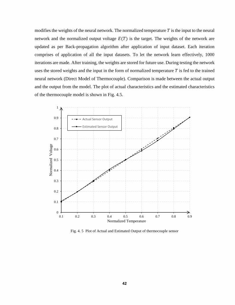
42
modifies the weights of the neural network. The normalized temperature 𝑇 is the input to the neural
network and the normalized output voltage 𝐸(𝑇) is the target. The weights of the network are
updated as per Back-propagation algorithm after application of input dataset. Each iteration
comprises of application of all the input datasets. To let the network learn effectively, 1000
iterations are made. After training, the weights are stored for future use. During testing the network
uses the stored weights and the input in the form of normalized temperature 𝑇 is fed to the trained
neural network (Direct Model of Thermocouple). Comparison is made between the actual output
and the output from the model. The plot of actual characteristics and the estimated characteristics
of the thermocouple model is shown in Fig. 4.5.
0
0.1
0.2
0.3
0.4
0.5
0.6
0.7
0.8
0.9
1
0.1 0.2 0.3 0.4 0.5 0.6 0.7 0.8 0.9
No
rmal
ized
V
olt
age
Normalized Temperature
Actual Sensor Output
Estimated Sensor Output
Fig. 4. 5 Plot of Actual and Estimated Output of thermocouple sensor
Page 52
43
4.3.2 Neural network based inverse modeling of thermocouple
Same structure 1-5-1 of the multilayer perceptron is used for the simulation of the inverse model
of the thermocouple. Similar training method is used to train the neural network. The network
training is done for 1000 iterations using Back-propagation algorithm and the adjusted weights are
stored in the memory. The only difference is the normalized voltage becomes the input and the
normalized temperature becomes the output. In testing of the inverse model, the thermocouple
output voltage 𝐸(𝑇) is applied to the network and the estimated temperature 𝑇 is obtained from
the neural model. The plots in case of neural model are shown in Fig. 4.6.
Fig. 4. 6 Plots of forward, inverse and overall characteristics of the thermocouple
Page 53
44
5
NEURAL NETWORK BASED SENSOR
LINEARIZATION
Page 54
45
5 NEURAL NETWORK BASED SENSOR
LINEARIZATION
Many sensors provide nonlinear input-output behavior. Analog circuits are used to improve the
nonlinearity of sensors. But sometimes the complex circuits along with the component tolerances
and temperature drift makes it impossible to used analog method of linearization. These days
microcomputer based systems are used for nonlinearity compensation of sensors. For
compensating the nonlinearity using arithmetic operations, an accurate model of the sensor is
required. The Look-up table is also used in micro-controller based applications but a large amount
of memory is required to attain high resolution. Neural network based sensor linearization can be
achieved by using comparatively less amount of memory and processing power. In neural network
based sensor linearization, a single input single output (SISO) multilayer perceptron network used
where input is the sensor measurement output data and the target is the corresponding desired
linear data [11]. Fig. 5.1 shows the block diagrams of the implementation of neural network based
linearization. Fig. 5.1(a) illustrates that the neural network is trained with nonlinear sensor
characteristics data as input and the desired linear characteristics data as target. Fig 5.1(b) shows
the sensor output 𝑉𝑛𝑙 is input to the neural network that produces corresponding linear output 𝑉𝑙.
Fig. 5. 1 Neural Network based Linearization (a) Training and (b) Testing
Sensor Neural
Network
Neural Network
𝑉𝑛𝑙 𝑉𝑙
(a)
(b)
𝑉𝑛𝑙 𝑉′𝑙 𝑇
Page 55
46
5.1 Simulation Results
The voltage divider circuit of Fig. 3.2 is used to obtain the nonlinear voltage 𝑉𝑛𝑙 which reflects the
temperature sensed by the thermistor. For the purpose of simulation study, a two layer multilayer
perceptron with 1-5-1 structure similar to Fig. 2.6 is used. The normalized nonlinear output voltage
𝑉𝑛𝑙 is applied as an input to the network and the normalized desired linear voltage 𝑉𝑙 is used as the
target neural network training. All the other parameters and operations to train the neural network
are similar to those discussed in section 3.4.1. After training, the weights are stored for future use.
During the testing of network the stored weights are used in the network and the normalized
nonlinear output voltage 𝑉𝑛𝑙 is fed to the trained neural network. Comparison is made between the
output from the neural network 𝑉𝑙 and the actual output to study the effectiveness of the network.
The plots of actual nonlinear characteristics of the sensor and the estimated linear characteristics
of the neural network are shown in Fig. 5.2.
0
0.1
0.2
0.3
0.4
0.5
0.6
0.7
0.8
0.9
1
0 0.1 0.2 0.3 0.4 0.5 0.6 0.7 0.8 0.9
No
rmal
ized
V
olt
age
Normalized Temperature
Nonlinear Voltage
Linearized Voltage
Fig. 5. 2 Characteristics of the sensor before and after linearization suing neural network
Page 57
48
6 CONCLUSION
The direct and the inverse model of thermistor as well as thermocouple are designed using neural
network technique. The direct model of the thermistor shows the performance similar to the actual
sensor. The direct model can be used in the detection of faults in the sensor. The nonlinearity issue
of the thermistor can be compensated by using the inverse model of the thermistor. The overall
response of the thermistor sensor circuit in series with the inverse model of the thermistor is linear
which shows the nonlinearity compensation. Similar models are developed for thermocouple.
Thermocouple is nonlinear when its operating range is extended. So inverse model is developed
which removes such nonlinearity. Another method to get rid of nonlinearity of thermistor is by
using the desired linear output voltage as the target of the neural network and the nonlinear output
voltage as an input to the neural network. In this method, the output voltage obtained is in linear
relationship with the temperature.
The models designed using the neural network are having very simple architecture. Such models
can be implemented in simple microcontrollers reducing the cost of the system. The development
of the model is done using the supervised learning. In applications where the training data is not
available, unsupervised learning can be carried out. The sensors used in this work are thermistors
and thermocouples. This technique can be applied to other sensors with more than one input to
affect the output of the sensor.
Page 58
49
BIBLIOGRAPHY
[1] D. Patranabis, S. Ghosh, C. Bakshi, “Linearizing transducer characteristics,” IEEE
Trans. Instrum. Meas., vol.37, no.1, pp. 66-69, 1988.
[2] N. Medrano-Marqués, R. del-Hoyo-Alonso, B. Martín-del-Brío, “A Thermocouple
Model Based on Neural Networks”, 6th International Work-Conference on Artificial
and Natural Neural Networks (IWANN) Spain, pp. 531-538, 2001.
[3] Medrano-Marques, N.J., Martin-del-Brio, B., “Sensor linearization with neural
networks,” IEEE Trans. Ind. Elect., vol.48, no.6, pp. 1288-1290, 2001.
[4] M. Attari, F. Boudema, M. Heniche; “An Artificial Neural Network to linearize a G
(Tungsten vs. Tungsten 26% Rhenium) Thermocouple characteristic in the range of
zero to 2000°C,” IEEE International Symposium on Circuits and Systems
[5] K. Danisman, I. Dalkiran, F.V. Celebi, “Design of a high precision temperature
measurement system based on artificial neural networks for different thermocouple
types,” Measurement, vol.39, no.8, pp 695-700, 2006.
[6] Dempsey, G.L., Alt, N.L., Olson, B.A., Alig, J.S., “Control sensor linearization using
microcontroller-based neural network,” Proc. of IEEE Conference on Systems, Man
and Cybernetics, vol.4, pp. 3078-3083, 1997.
[7] L. R. Klopfenstein, “Software linearization technique for thermocouples, thermistors
and RTDs,” ISA Trans., vol.33, no.3, pp. 293-305, 1994.
[8] Obaidat, M.S., Abu-Saymeh, D.S., “Methodologies for characterizing ultrasonic
transducers using neural networks and pattern recognition techniques,” IEEE Trans.
Ind.. Elect., vol.39, no.6, pp. 529-536, 1992.
[9] J.C. Patra, G. Panda and R. Baliarsingh, “Artificial neural network based nonlinearity
estimation of pressure sensors,” IEEE Trans. Instrumentation & Measurement, vol.43,
pp.874-881, Dec.1994.
Page 59
50
[10] Haykin, S., Neural Networks and Learning Machines, 3rd edition New Delhi,
Prentice Hall, 2011.
[11] Bhuyan, M., Intelligent Instrumentation, Florida, CRC Press, 2011.
[12] National Institute of Science and Technology (NIST) ITS-90 Thermocouple Database.
Available: http://www.srdata.nist.gov/its90/download/type_k.tab