15
Probability Operations: Mean, Variance & Expectation Describing random events. 1
| Date post: | 19-Jul-2016 |
| Category: |
Documents |
| Upload: | roberto-antonioli |
| View: | 12 times |
| Download: | 4 times |

Probability Operations: Mean, Variance & Expectation
Describing random events.
1

2
The probable is what usually happens.
Aristotle

Recall: Probability Distribution/Mass Function
The distribution of the probability mass function of a discrete r.v. is defined for every number x such that[1]:
4
𝑝 𝑥 = 𝑃 𝑋 = 𝑥 = 𝑃 𝑎𝑙𝑙 𝑠 ∈ 𝑆: 𝑋 𝑠 = 𝑥Depends on the mapping of the event space to the random variable
𝑥
𝑝 𝑥 = 1 −∞
∞
𝑝 𝑥 𝑑𝑥 = 1
Discrete Distribution Continuous Distribution
[1] Devore, J.L., Probability and Statistics for Engineering and the Sciences 5th Edition, Duxbury, Pacific Grove, pg 101
Under the condition that: and 𝑝(𝑥) ≥ 0

Characterizing a Random Variable
The probability density function gives a very detailed description of a random variable but:
• It may not be that compact.
• It is difficult to compare two different r.v.s.
What are some techniques for summarizing the properties of a random variable?
5
𝐸 𝑋 = 𝜇 =
𝑥∈𝐷
𝑥 ∙ 𝑝(𝑥)
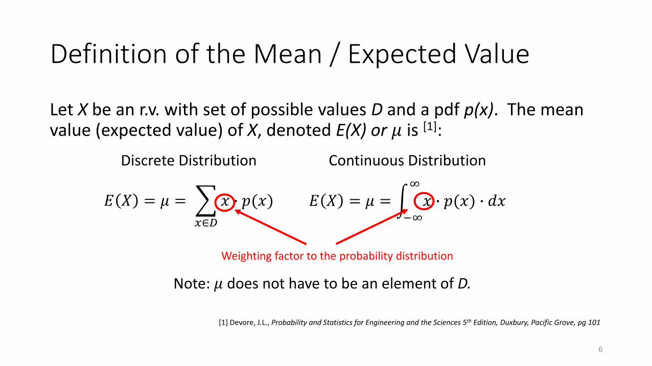
Definition of the Mean / Expected Value
Let X be an r.v. with set of possible values D and a pdf p(x). The mean value (expected value) of X, denoted E(X) or 𝜇 is [1]:
6
𝐸 𝑋 = 𝜇 = −∞
∞
𝑥 ∙ 𝑝(𝑥) ∙ 𝑑𝑥
Discrete Distribution Continuous Distribution
Note: 𝜇 does not have to be an element of D.
[1] Devore, J.L., Probability and Statistics for Engineering and the Sciences 5th Edition, Duxbury, Pacific Grove, pg 101
Weighting factor to the probability distribution

Definition of Variance
Let X have a pdf p(x) and an expected value 𝜇. The variance of X, denoted by V(X) or 𝜎𝑋
2, is:
7
V(𝑋) = 𝜎𝑋2= 𝐷 𝑥 − 𝜇
2 ∙ 𝑝(𝑥) V(𝑋) = 𝜎𝑋2= −∞∞𝑥 − 𝜇 2 ∙ 𝑝(𝑥) ∙ 𝑑𝑥
Discrete Distribution Continuous Distribution
Weighting factor to the probability distribution
V(𝑋) = 𝐸 𝑋 − 𝜇 2 = 𝐸 𝑋2 − 𝜇 2
Measure of variation around the mean.

What is six sigma?Six Sigma is a set of techniques and tools for process improvement. It was developed by Motorola in 1986.
Improves the quality of process outputs by identifying and removing the causes of defects (errors) and minimizing variability in manufacturing and business processes.
8

Standard Deviation (Root-Mean-Square)
9
Range ConfidenceInterval
𝜎 0.6826895
2𝜎 0.9544997
3𝜎 0.9973002
4𝜎 0.9999366
′6𝜎′=4.5𝜎 0.9999966
5𝜎 0.9999994www.six-sigma-material.com/Normal-Distribution.html
Normal (Gaussian) Distribution
Many distributions or processes can be approximated as Gaussian – useful for analysis.
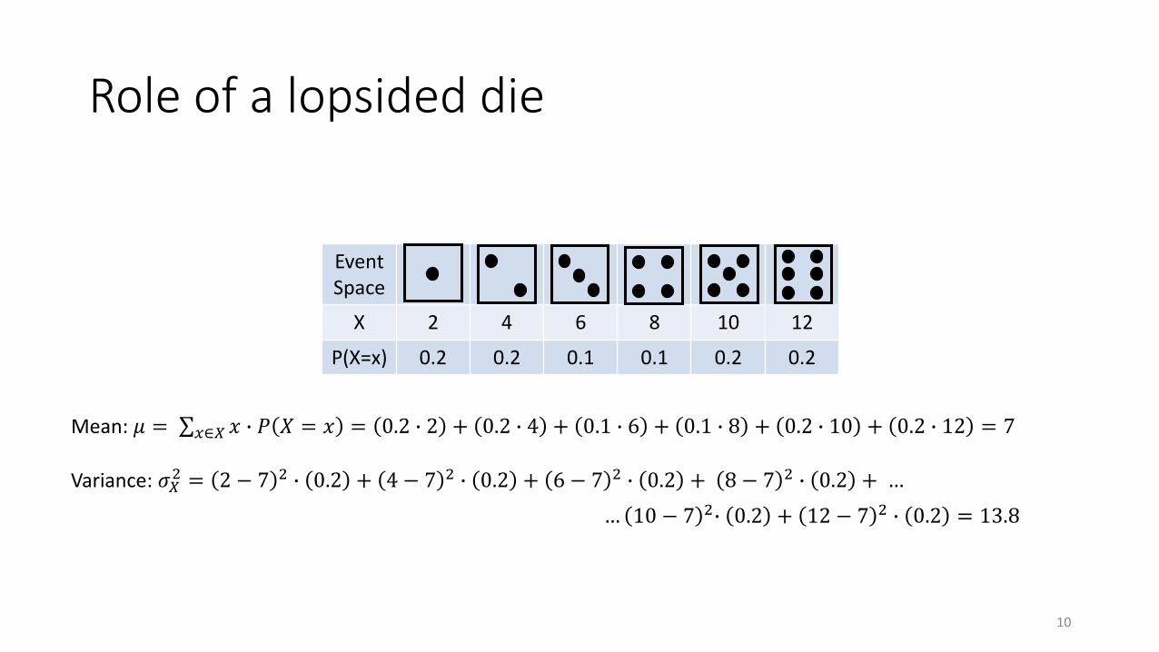
Role of a lopsided die
10
Mean: 𝜇 = 𝑥∈𝑋 𝑥 ∙ 𝑃 𝑋 = 𝑥 = 0.2 ∙ 2 + 0.2 ∙ 4 + 0.1 ∙ 6 + 0.1 ∙ 8 + 0.2 ∙ 10 + 0.2 ∙ 12 = 7
Variance: 𝜎𝑋2 = 2 − 7 2 ∙ 0.2 + 4 − 7 2 ∙ 0.2 + 6 − 7 2 ∙ 0.2 + 8 − 7 2 ∙ 0.2 + …
… 10 − 7 2∙ 0.2 + 12 − 7 2 ∙ 0.2 = 13.8
EventSpace
X 2 4 6 8 10 12
P(X=x) 0.2 0.2 0.1 0.1 0.2 0.2

Building some intuition (1) …
11
(2) Variance
< A
= B
> C
(1) Mean
< A
= B
> C

Building some intuition (2)…
12
(2) Variance
< A
= B
> C
(1) Mean
< A
= B
> C
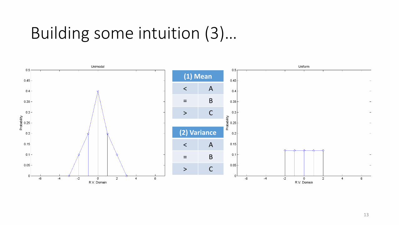
Building some intuition (3)…
13
(2) Variance
< A
= B
> C
(1) Mean
< A
= B
> C
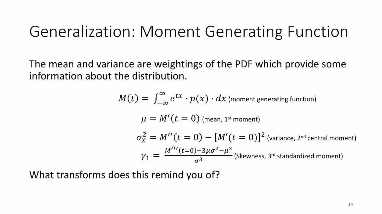
Generalization: Moment Generating Function
The mean and variance are weightings of the PDF which provide some information about the distribution.
14
𝑀 𝑡 = −∞∞𝑒𝑡𝑥 ∙ 𝑝(𝑥) ∙ 𝑑𝑥 (moment generating function)
𝜇 = 𝑀′ 𝑡 = 0 (mean, 1st moment)
𝜎𝑋2 = 𝑀′′ 𝑡 = 0 − 𝑀′(𝑡 = 0) 2 (variance, 2nd central moment)
What transforms does this remind you of?
𝛾1 =𝑀′′′ 𝑡=0 −3𝜇𝜎2−𝜇3
𝜎3(Skewness, 3rd standardized moment)

Importance to the course
The concept of weighting a ‘root’ function is central to the description and analysis of communication systems:
1. Weighting of probability functions to describe distributions (mean, variance).
2. Laplace transform for modeling the behaviour of circuits, control and stability (less significant in this course).
3. Fourier transform for representing signals, noise and filters.
15

Learning Outcomes
1. Apply mean and variance definitions to probability distributions.
2. Heuristic understanding of the definitions of mean and variance as it applies to probability distributions.
16


