Title

TIK-Schriftenreihe Nr. 39

Hans Otto Trutmann

Separate Connection andFunctionality is the Pivotin Embedded System Design

A dissertation submitted to theSwiss Federal Institute of Technology ETH Zürichfor the degree of Doctor of Technical Sciences

Diss. ETH No. 13891

Prof. Dr. Albert Kündig, examinerProf. Dr. Matjaz Colnaric, co-examiner

Examination date: October 23, 2000

© 2000 Institut für Technische Informatik und Kommunikationsnetze TIK, ETH Zürich

ISBN 3-906469-09-3

Preface

to J. H. W. & M. E.

Preface

The present publication marks the end of my time at the Computer Engineer-ing and Networks Laboratory TIK of ETH Zürich. Beginning in 1989, foreight years my main focus has been the control system for the Hybrid III car.Apart from theoretical and conceptual questions, this has proven a comprehen-sive task with many practical aspects. It offered the chance for trying newlyfound concepts in a demanding real-world application. This thesis expands andgeneralizes these ideas.

I thank everybody who helped me, especially my thesis supervisor Prof. AlbertKündig, who gave me the opportunity to work on this project. The laboratoryunder his prudent guidance provided the necessary freedom in the search formy own solutions. This freedom added a strong sentiment of responsibility fortheir functioning; it also augmented my pleasure when they actually worked.

I also thank my co-advisor Prof. Matjaz Colnaric for his interest and remarks.

Nebojsa Jelaca deserves my thanks for his continuing efforts in hardware devel-opment and his patience also in difficult times, Dr. Hugo Fierz for his friend-ship and for the intense cooperation and many interesting discussions about allfacets of embedded systems; the CIP method – developed by him and Hans-ruedi Müller – was one of the prerequisites for my work, and possibly also forthe success of Hybrid III. Valuable contributions were made by students,among them Matthias Manhart, Patrik Reali, Hanspeter Schmid and AndreasErne. Aside from all academic considerations, the touchstone for the envisagedsolutions has always been their applicability to real-world problems; therefore Imust also thank the Hybrid III team for having kept me in touch with theindustrial reality.

I thank all my family and friends for making my life interesting and enjoyable.Most of all, I thank my wife Veronica Bürgler and my daughter Eva for being asource of pleasure and for teaching me more than I ever learned elsewhere.

Zürich, October 2000

v

Abstract

The goal in the development of embedded real-time systems is a solution thatsatisfies the initial requirements, although this is not enough. There is also aneed for appropriate descriptions of the many different aspects of a system, forconnecting these representations among each other and with the implementa-tion itself, for easing maintenance and for dealing with organizational chores.All this makes the solution appear as a by-product of a well-organized develop-ment process. This development process profits from a clear separation of con-cerns, which can be achieved with an explicit interconnection model, thearchitectural pivot specification. Its relative stability allows development toprogress independently behind stable syntactic and semantic interfaces.

The three basic activities in control applications, input, processing and output,are dealt with individually within separate problem areas. A problem-orientedapproach postulates the use of suitable methods and tools for solving each ofthese issues, thus embodying different formal representations and explicitlywritten code on different levels of abstraction. Unison is achieved through gen-erators yielding code with defined generic properties that favor smooth andefficient implementation. The functional problem comprises all the behavioralaspects of a control system, using shared phenomena to interact with the con-trolled processes in the environment. Solutions to this problem omit anydetails not pertaining to the relation between the course of events in the envi-ronment and the inner states of a model. The connection problem is concernedwith information transport from and to the environment. Its solution is basedon regular sequential structures.

During development, the common high-level source baseline permits generat-ing implementations for various modes of operation without modifying theabstract descriptions. The approach eliminates manual programming whencode alterations are needed to adapt to changes in the hardware environment.It thus allows testing of proposed solutions against numerical models, as well asadapting resources according to emerging requirements any time during thedevelopment process. It supports decentralized development work and simpli-fies target implementations without complicated scheduling, without inter-rupts, and without the overhead of elaborate operating systems. The code isstatically deterministic, and the performance of entire implementations is ana-lyzed exhaustively to assure the desired real-time properties.

vi

Zusammenfassung

Das Ziel bei der Entwicklung eingebetteter Echtzeitsysteme ist eine der Anfor-derungsspezifikation genügende Lösung; das reicht jedoch noch nicht aus. Esbraucht auch den verschiedenen Aspekten angemessene Beschreibungen, Ver-bindungen dieser Beschreibungen untereinander und zur Implementation,Unterstützung beim Unterhalt, bei der Weiterentwicklung und beim organisa-torischen Ablauf. All das lässt die eigentliche Lösung dann eher als die Begleit-erscheinung eines gut organisierten Entwicklungsprozesses erscheinen. DieserProzess profitiert von klar voneinander abgegrenzten Problembereichen; eineAbgrenzung, die mit der architektonischen Pivot-Beschreibung erzielt wird.Hinter solch syntaktisch und semantisch stabilen Schnittstellen kann innerhalbeinzelner Problembereiche selbständig weiterentwickelt werden.

Die drei grundlegenden Aktivitäten in Steueranwendungen, Eingabe, Verarbei-tung und Ausgabe, werden gesondert in eigenen Problembereichen behandelt.Ein problembezogener Ansatz postuliert den Gebrauch geeigneter Methodenund Werkzeuge für jedes dieser Gebiete, so dass es verschiedene formale Dar-stellungen neben explizit geschriebenem Programmtext auf mehreren Abstrak-tionsstufen gibt. Diese werden mittels Generatoren vereinigt, welche Code mitdefinierten generischen Eigenschaften liefern, der sich einfach und effizientimplementieren lässt. Das funktionale Problem umfasst das Systemverhalten;die Koppelung des Steuersystems mit den zu steuernden Prozessen in derUmgebung läuft über Phänomene, welche von beiden geteilt werden, so dassLösungen dieses Problems nur die Wechselbeziehung von Ereignisfolgen in derUmgebung mit dem inneren Zustand des Modells beinhalten. Beim Verbin-dungsproblem geht es um den Transport von Information vom und zum kon-trollierten Prozess. Lösungen basieren hier auf sequentiellen Strukturen.

Aus den gemeinsamen abstrakten Beschreibungen lassen sich Implementatio-nen für verschiedenste Betriebsarten generieren, was manuelle Eingriffe beimAustausch von Systemkomponenten überflüssig macht. Die erarbeitetenLösungen können an numerischen Anlagemodellen ausprobiert werden. DerAnsatz unterstützt die dezentrale Entwicklung von Systemen und vereinfachtdie Installation auf dem Zielsystem: keine komplizierte Ablaufplanung, keineUnterbrechungen und kein aufwendiges Betriebssystem. Der erzeugte Code iststatisch deterministisch, und das Zeitverhalten von ganzen Implementationenwird umfassend geprüft, um das gewünschte Echtzeitverhalten nachzuweisen.

vii

viii

Contents

1 Introduction . . . . . . . . . . . . . . . . . . . . . . . . . . . . . . . . . . . . . . . . . . . . . . . . . . . . . . . . 1

1.1 Development Concepts . . . . . . . . . . . . . . . . . . . . . . . . . . . . . . . . . . . . . . . . . . . 61.1.1 Separation of Concerns . . . . . . . . . . . . . . . . . . . . . . . . . . . . . . . . . . . . . . 61.1.2 Development Emphasis . . . . . . . . . . . . . . . . . . . . . . . . . . . . . . . . . . . . . . 7

1.2 The Toolbox . . . . . . . . . . . . . . . . . . . . . . . . . . . . . . . . . . . . . . . . . . . . . . . . . . 10

1.3 Overview . . . . . . . . . . . . . . . . . . . . . . . . . . . . . . . . . . . . . . . . . . . . . . . . . . . . . 11

2 Embedded Systems . . . . . . . . . . . . . . . . . . . . . . . . . . . . . . . . . . . . . . . . . . . . . . . . . . 15

2.1 Requirements . . . . . . . . . . . . . . . . . . . . . . . . . . . . . . . . . . . . . . . . . . . . . . . . . . 172.1.1 Functional Requirements . . . . . . . . . . . . . . . . . . . . . . . . . . . . . . . . . . . 182.1.2 Temporal Requirements . . . . . . . . . . . . . . . . . . . . . . . . . . . . . . . . . . . . 192.1.3 Accuracy Requirements . . . . . . . . . . . . . . . . . . . . . . . . . . . . . . . . . . . . . 242.1.4 Implementation Requirements . . . . . . . . . . . . . . . . . . . . . . . . . . . . . . . 252.1.5 Communication Requirements . . . . . . . . . . . . . . . . . . . . . . . . . . . . . . . 262.1.6 Reliability Requirements . . . . . . . . . . . . . . . . . . . . . . . . . . . . . . . . . . . . 28

2.2 Development . . . . . . . . . . . . . . . . . . . . . . . . . . . . . . . . . . . . . . . . . . . . . . . . . . 302.2.1 Building Principles . . . . . . . . . . . . . . . . . . . . . . . . . . . . . . . . . . . . . . . . 312.2.2 Architecture . . . . . . . . . . . . . . . . . . . . . . . . . . . . . . . . . . . . . . . . . . . . . . 322.2.3 Language Issues . . . . . . . . . . . . . . . . . . . . . . . . . . . . . . . . . . . . . . . . . . . 342.2.4 Tools . . . . . . . . . . . . . . . . . . . . . . . . . . . . . . . . . . . . . . . . . . . . . . . . . . . 362.2.5 Modes of Operation . . . . . . . . . . . . . . . . . . . . . . . . . . . . . . . . . . . . . . . 372.2.6 Simulation . . . . . . . . . . . . . . . . . . . . . . . . . . . . . . . . . . . . . . . . . . . . . . . 382.2.7 Performance Verification . . . . . . . . . . . . . . . . . . . . . . . . . . . . . . . . . . . . 39

2.3 Deployment Techniques . . . . . . . . . . . . . . . . . . . . . . . . . . . . . . . . . . . . . . . . . 402.3.1 Deployment . . . . . . . . . . . . . . . . . . . . . . . . . . . . . . . . . . . . . . . . . . . . . 402.3.2 Code Generation . . . . . . . . . . . . . . . . . . . . . . . . . . . . . . . . . . . . . . . . . . 422.3.3 Resource Management . . . . . . . . . . . . . . . . . . . . . . . . . . . . . . . . . . . . . 432.3.4 Communication . . . . . . . . . . . . . . . . . . . . . . . . . . . . . . . . . . . . . . . . . . 46

3 Problem Decomposition . . . . . . . . . . . . . . . . . . . . . . . . . . . . . . . . . . . . . . . . . . . . . . 49

3.1 Architectures . . . . . . . . . . . . . . . . . . . . . . . . . . . . . . . . . . . . . . . . . . . . . . . . . . 50

3.2 Separation of Concerns . . . . . . . . . . . . . . . . . . . . . . . . . . . . . . . . . . . . . . . . . . 513.2.1 Functional Problem Frame . . . . . . . . . . . . . . . . . . . . . . . . . . . . . . . . . . 54

ix

Contents

3.2.2 Connection Problem Frame . . . . . . . . . . . . . . . . . . . . . . . . . . . . . . . . . 553.2.3 Classification . . . . . . . . . . . . . . . . . . . . . . . . . . . . . . . . . . . . . . . . . . . . . 57

3.3 Abstraction . . . . . . . . . . . . . . . . . . . . . . . . . . . . . . . . . . . . . . . . . . . . . . . . . . . 58

3.4 Practical Development Suites . . . . . . . . . . . . . . . . . . . . . . . . . . . . . . . . . . . . . . 60

4 Architecture . . . . . . . . . . . . . . . . . . . . . . . . . . . . . . . . . . . . . . . . . . . . . . . . . . . . . . . . 61

4.1 Operational Architecture . . . . . . . . . . . . . . . . . . . . . . . . . . . . . . . . . . . . . . . . . 62

4.2 Implementation Architecture . . . . . . . . . . . . . . . . . . . . . . . . . . . . . . . . . . . . . . 64

4.3 Component Architecture . . . . . . . . . . . . . . . . . . . . . . . . . . . . . . . . . . . . . . . . . 664.3.1 Specification . . . . . . . . . . . . . . . . . . . . . . . . . . . . . . . . . . . . . . . . . . . . . 684.3.2 Components . . . . . . . . . . . . . . . . . . . . . . . . . . . . . . . . . . . . . . . . . . . . . 684.3.3 Connectors . . . . . . . . . . . . . . . . . . . . . . . . . . . . . . . . . . . . . . . . . . . . . . 714.3.4 The Pivot . . . . . . . . . . . . . . . . . . . . . . . . . . . . . . . . . . . . . . . . . . . . . . . 73

5 Functionality . . . . . . . . . . . . . . . . . . . . . . . . . . . . . . . . . . . . . . . . . . . . . . . . . . . . . . . 75

5.1 State Machine Models . . . . . . . . . . . . . . . . . . . . . . . . . . . . . . . . . . . . . . . . . . . 765.1.1 Finite State Machines . . . . . . . . . . . . . . . . . . . . . . . . . . . . . . . . . . . . . . 765.1.2 Hierarchy . . . . . . . . . . . . . . . . . . . . . . . . . . . . . . . . . . . . . . . . . . . . . . . 785.1.3 Cooperation . . . . . . . . . . . . . . . . . . . . . . . . . . . . . . . . . . . . . . . . . . . . . 785.1.4 State Machine Extension . . . . . . . . . . . . . . . . . . . . . . . . . . . . . . . . . . . . 785.1.5 Semantics . . . . . . . . . . . . . . . . . . . . . . . . . . . . . . . . . . . . . . . . . . . . . . . 79

5.2 Communicating Interacting Processes CIP . . . . . . . . . . . . . . . . . . . . . . . . . . . 80

5.3 CIP Constructive Elements . . . . . . . . . . . . . . . . . . . . . . . . . . . . . . . . . . . . . . . 825.3.1 Process . . . . . . . . . . . . . . . . . . . . . . . . . . . . . . . . . . . . . . . . . . . . . . . . . . 825.3.2 Synchronous and Asynchronous Cooperation . . . . . . . . . . . . . . . . . . . . 835.3.3 Behavioral Structuring . . . . . . . . . . . . . . . . . . . . . . . . . . . . . . . . . . . . . . 865.3.4 Extensions . . . . . . . . . . . . . . . . . . . . . . . . . . . . . . . . . . . . . . . . . . . . . . . 88

5.4 CIP Implementation Units . . . . . . . . . . . . . . . . . . . . . . . . . . . . . . . . . . . . . . . 90

5.5 Working with CIP Models . . . . . . . . . . . . . . . . . . . . . . . . . . . . . . . . . . . . . . . . 925.5.1 Functional Models within a Context . . . . . . . . . . . . . . . . . . . . . . . . . . . 925.5.2 Initialization . . . . . . . . . . . . . . . . . . . . . . . . . . . . . . . . . . . . . . . . . . . . . 955.5.3 An Eye on Interaction . . . . . . . . . . . . . . . . . . . . . . . . . . . . . . . . . . . . . . 955.5.4 Behavioral Patterns . . . . . . . . . . . . . . . . . . . . . . . . . . . . . . . . . . . . . . . . 96

6 Connection . . . . . . . . . . . . . . . . . . . . . . . . . . . . . . . . . . . . . . . . . . . . . . . . . . . . . . . . 97

6.1 Device Access . . . . . . . . . . . . . . . . . . . . . . . . . . . . . . . . . . . . . . . . . . . . . . . . . . 996.1.1 Representation of Continuous Signals . . . . . . . . . . . . . . . . . . . . . . . . . 1016.1.2 Encoding of Discrete Values . . . . . . . . . . . . . . . . . . . . . . . . . . . . . . . . 102

6.2 Data Acquisition . . . . . . . . . . . . . . . . . . . . . . . . . . . . . . . . . . . . . . . . . . . . . . 103

6.3 Input Data Distribution . . . . . . . . . . . . . . . . . . . . . . . . . . . . . . . . . . . . . . . . . 108

6.4 Event Extraction . . . . . . . . . . . . . . . . . . . . . . . . . . . . . . . . . . . . . . . . . . . . . . 111

6.5 Output . . . . . . . . . . . . . . . . . . . . . . . . . . . . . . . . . . . . . . . . . . . . . . . . . . . . . . 112

6.6 Communication . . . . . . . . . . . . . . . . . . . . . . . . . . . . . . . . . . . . . . . . . . . . . . . 114

x

Contents

7 Implementation . . . . . . . . . . . . . . . . . . . . . . . . . . . . . . . . . . . . . . . . . . . . . . . . . . . . 115

7.1 Code . . . . . . . . . . . . . . . . . . . . . . . . . . . . . . . . . . . . . . . . . . . . . . . . . . . . . . . . 1177.1.1 Functional Code . . . . . . . . . . . . . . . . . . . . . . . . . . . . . . . . . . . . . . . . . 1177.1.2 Connection Code . . . . . . . . . . . . . . . . . . . . . . . . . . . . . . . . . . . . . . . . . 120

7.2 Deployment . . . . . . . . . . . . . . . . . . . . . . . . . . . . . . . . . . . . . . . . . . . . . . . . . . 1217.2.1 Scheduling . . . . . . . . . . . . . . . . . . . . . . . . . . . . . . . . . . . . . . . . . . . . . . 1227.2.2 Processing Scheduler . . . . . . . . . . . . . . . . . . . . . . . . . . . . . . . . . . . . . . 1237.2.3 Implementation Variants . . . . . . . . . . . . . . . . . . . . . . . . . . . . . . . . . . . 124

7.3 Dynamic Reconfiguration . . . . . . . . . . . . . . . . . . . . . . . . . . . . . . . . . . . . . . . 1287.3.1 Static Approach . . . . . . . . . . . . . . . . . . . . . . . . . . . . . . . . . . . . . . . . . . 1287.3.2 Reconfiguration Strategy . . . . . . . . . . . . . . . . . . . . . . . . . . . . . . . . . . . 1307.3.3 Example . . . . . . . . . . . . . . . . . . . . . . . . . . . . . . . . . . . . . . . . . . . . . . . . 131

8 Hybrid III . . . . . . . . . . . . . . . . . . . . . . . . . . . . . . . . . . . . . . . . . . . . . . . . . . . . . . . . . 135

8.1 Hybrid Vehicles . . . . . . . . . . . . . . . . . . . . . . . . . . . . . . . . . . . . . . . . . . . . . . . 1358.1.1 Hybrid Concepts . . . . . . . . . . . . . . . . . . . . . . . . . . . . . . . . . . . . . . . . . 1368.1.2 Drive Systems and Energy Storage Devices . . . . . . . . . . . . . . . . . . . . . 137

8.2 The Project Hybrid III . . . . . . . . . . . . . . . . . . . . . . . . . . . . . . . . . . . . . . . . . . 1388.2.1 How it Works . . . . . . . . . . . . . . . . . . . . . . . . . . . . . . . . . . . . . . . . . . . 1408.2.2 Results . . . . . . . . . . . . . . . . . . . . . . . . . . . . . . . . . . . . . . . . . . . . . . . . . 140

8.3 Hybrid III Components . . . . . . . . . . . . . . . . . . . . . . . . . . . . . . . . . . . . . . . . . 141

9 Hybrid III Control . . . . . . . . . . . . . . . . . . . . . . . . . . . . . . . . . . . . . . . . . . . . . . . . . . 145

9.1 Concepts . . . . . . . . . . . . . . . . . . . . . . . . . . . . . . . . . . . . . . . . . . . . . . . . . . . . 1479.1.1 Processors . . . . . . . . . . . . . . . . . . . . . . . . . . . . . . . . . . . . . . . . . . . . . . . 1489.1.2 Communication . . . . . . . . . . . . . . . . . . . . . . . . . . . . . . . . . . . . . . . . . . 1509.1.3 Input and Output . . . . . . . . . . . . . . . . . . . . . . . . . . . . . . . . . . . . . . . . 1529.1.4 Bus Systems . . . . . . . . . . . . . . . . . . . . . . . . . . . . . . . . . . . . . . . . . . . . . 1549.1.5 Mechanical and Electrical Installation . . . . . . . . . . . . . . . . . . . . . . . . . 1549.1.6 Code . . . . . . . . . . . . . . . . . . . . . . . . . . . . . . . . . . . . . . . . . . . . . . . . . . 155

9.2 Methods and Tools . . . . . . . . . . . . . . . . . . . . . . . . . . . . . . . . . . . . . . . . . . . . . 1569.2.1 Working Environment . . . . . . . . . . . . . . . . . . . . . . . . . . . . . . . . . . . . . 1579.2.2 Configuration and Modeling . . . . . . . . . . . . . . . . . . . . . . . . . . . . . . . . 158

9.3 Hardware Implementation . . . . . . . . . . . . . . . . . . . . . . . . . . . . . . . . . . . . . . . 1609.3.1 Control System . . . . . . . . . . . . . . . . . . . . . . . . . . . . . . . . . . . . . . . . . . 1609.3.2 Peripherals . . . . . . . . . . . . . . . . . . . . . . . . . . . . . . . . . . . . . . . . . . . . . . 1629.3.3 Additional Hardware . . . . . . . . . . . . . . . . . . . . . . . . . . . . . . . . . . . . . . 162

9.4 Software Implementation . . . . . . . . . . . . . . . . . . . . . . . . . . . . . . . . . . . . . . . . 1649.4.1 Communication . . . . . . . . . . . . . . . . . . . . . . . . . . . . . . . . . . . . . . . . . . 1649.4.2 System Software and Connection . . . . . . . . . . . . . . . . . . . . . . . . . . . . . 1659.4.3 Functional Code . . . . . . . . . . . . . . . . . . . . . . . . . . . . . . . . . . . . . . . . . 170

10 Conclusions . . . . . . . . . . . . . . . . . . . . . . . . . . . . . . . . . . . . . . . . . . . . . . . . . . . . . . 171

10.1 Complete Solutions . . . . . . . . . . . . . . . . . . . . . . . . . . . . . . . . . . . . . . . . . . . 173

10.2 Implementation . . . . . . . . . . . . . . . . . . . . . . . . . . . . . . . . . . . . . . . . . . . . . . 174

10.3 Reuse . . . . . . . . . . . . . . . . . . . . . . . . . . . . . . . . . . . . . . . . . . . . . . . . . . . . . . 175

10.4 Suggestions for Further Work . . . . . . . . . . . . . . . . . . . . . . . . . . . . . . . . . . . . 175

xi

Contents

A Specification . . . . . . . . . . . . . . . . . . . . . . . . . . . . . . . . . . . . . . . . . . . . . . . . . . . . . . 177

A.1 Architectural Specification . . . . . . . . . . . . . . . . . . . . . . . . . . . . . . . . . . . . . . . 178A.1.1 Specification Language . . . . . . . . . . . . . . . . . . . . . . . . . . . . . . . . . . . . 178A.1.2 Productions . . . . . . . . . . . . . . . . . . . . . . . . . . . . . . . . . . . . . . . . . . . . . 179

A.2 Input and Output Specification . . . . . . . . . . . . . . . . . . . . . . . . . . . . . . . . . . . 183A.2.1 The Generator ‘acc’ . . . . . . . . . . . . . . . . . . . . . . . . . . . . . . . . . . . . . . . 183A.2.2 Specification Language . . . . . . . . . . . . . . . . . . . . . . . . . . . . . . . . . . . . 183A.2.3 Productions . . . . . . . . . . . . . . . . . . . . . . . . . . . . . . . . . . . . . . . . . . . . . 184

A.3 Event Extraction Specification . . . . . . . . . . . . . . . . . . . . . . . . . . . . . . . . . . . . 189A.3.1 The Generator ‘evt’ . . . . . . . . . . . . . . . . . . . . . . . . . . . . . . . . . . . . . . . 189A.3.2 Specification Language . . . . . . . . . . . . . . . . . . . . . . . . . . . . . . . . . . . . 190A.3.3 Productions . . . . . . . . . . . . . . . . . . . . . . . . . . . . . . . . . . . . . . . . . . . . . 190

A.4 Code Generator Program Structure . . . . . . . . . . . . . . . . . . . . . . . . . . . . . . . . 193A.4.1 Data Structures . . . . . . . . . . . . . . . . . . . . . . . . . . . . . . . . . . . . . . . . . . 194A.4.2 APs (Access Procedures) . . . . . . . . . . . . . . . . . . . . . . . . . . . . . . . . . . . 197A.4.3 IPs (Initialization Procedures) . . . . . . . . . . . . . . . . . . . . . . . . . . . . . . . 198A.4.4 Variables . . . . . . . . . . . . . . . . . . . . . . . . . . . . . . . . . . . . . . . . . . . . . . . 198A.4.5 Access Distribution . . . . . . . . . . . . . . . . . . . . . . . . . . . . . . . . . . . . . . . 199

B Syntax . . . . . . . . . . . . . . . . . . . . . . . . . . . . . . . . . . . . . . . . . . . . . . . . . . . . . . . . . . . 203

B.1 Architecture . . . . . . . . . . . . . . . . . . . . . . . . . . . . . . . . . . . . . . . . . . . . . . . . . . 203

B.2 Input and Output . . . . . . . . . . . . . . . . . . . . . . . . . . . . . . . . . . . . . . . . . . . . . 204

B.3 Event . . . . . . . . . . . . . . . . . . . . . . . . . . . . . . . . . . . . . . . . . . . . . . . . . . . . . . . 205

C Glossary . . . . . . . . . . . . . . . . . . . . . . . . . . . . . . . . . . . . . . . . . . . . . . . . . . . . . . . . . 207

References . . . . . . . . . . . . . . . . . . . . . . . . . . . . . . . . . . . . . . . . . . . . . . . . . . . . . . . . . . 221

List of Figures . . . . . . . . . . . . . . . . . . . . . . . . . . . . . . . . . . . . . . . . . . . . . . . . . . . . . . . 230

List of Tables . . . . . . . . . . . . . . . . . . . . . . . . . . . . . . . . . . . . . . . . . . . . . . . . . . . . . . . 233

Index . . . . . . . . . . . . . . . . . . . . . . . . . . . . . . . . . . . . . . . . . . . . . . . . . . . . . . . . . . . . . . 235

xii

1 Introduction

In our daily life we are surrounded by complex technical structures, most of thetime without worrying about their safety and dependability. We are secure inthe knowledge that buildings, bridges and means of transportation are basedon the principles of sound engineering. In recent years we have exposed our-selves increasingly, and with the same trust, to the influences of complex com-puter programs, although we would be well advised to exercise more caution inthis area. Contrary to disciplines like mechanical or electrical engineering, soft-ware engineering is in its infancy. It still lacks generally accepted ways and prin-ciples that would provide a reference frame for evaluating new solutions, and awide gap remains between practitioners whose interest is to build and use com-puter controlled systems, and computer scientists who study the mathematicsneeded to analyze systems and programs [Par97]. Because the scientists whostudy programming understand little about the problems of engineering, theyfail to explain how their proposed concepts could be put to use in real-worldapplications. If a solution demonstrated on toy problems does not scale, or if itneglects all the accessories needed to make this solution work, its possibilitiesare lost on practitioners. The products being built reflect this situation; they aredeveloped by people whose actual job is not programming, but who need toprogram in order to carry out some other task; therefore, these products oftenpresent a major source of problems for those who depend on them. So, theundeniable advantages such as enhanced functionality, flexibility and cheaperproduction of computer controls come at a great cost and risk. On the onehand, an increasing number of serious incidents, often accompanied by signifi-cant human and financial losses, can be traced back to computer failures[Risks]. On the other hand, software development makes up an increasingshare of the overall costs. If we are unable to develop a true engineering disci-pline with universal criteria in this area, then at least we have to ask how theexisting methods can be put to effective use: what is the best possible way todevelop systems that are reliable and cost-advantageous?

1

1 Introduction

Since the time when electronic systems were introduced, applications havecontinuously become more complicated. This in turn entailed more demand-ing requirements with regard to the quality of such solutions and, simulta-neously, to the quality of the development methods themselves. Unfortunatelyit seems as if all progress in this area is swallowed up by the growing complexityof the applications and by user demand that increases at an equal pace. Add tothis the fact that software fails differently from mechanical systems. Mechanicalsystems and their ability to continue functioning to a certain extent even in thecase of failure are in stark contrast to the infamous erroneous bit that unexpect-edly paralyzes an entire system. Redundancy and the ability to gracefullydegrade its functions were inherent in earlier controls in addition to the speci-fied functionality and significantly contributed to the safety of a system. In thechange over to computer solutions these features must be replicated or replacedentirely by different mechanisms. Regrettably this also does away with the pre-vious separation between normal operation and the operation in the presenceof failures. To make matters worse, it is not uncommon that the effortsrequired to manage these deviations far exceed those of the control task in nor-mal operation.

The newly gained vast expressive power and flexibility in turn propagate moreextensive requirements and result in complex implementations that are hard tocontrol. While the individual developers themselves have not become muchwiser during this process, the accumulated knowledge surrounding these issuesgrew immensely at the same time. For this reason, many developments nowa-days require the commitment of numerous specialists in a process in which allteam members pitch in to bring it to fruition. Cooperation, this oldest ofapproaches in resolving complex problems is reaching its limits, and the searchfor alternatives is getting more attention. The insight that in some areas toolsalready now have become indispensable has replaced the initial hopes of merelyincreasing productivity with the help of efficient tools. Contrary to humans,computer programs do become smarter in the course of time, as programs arecontinuously expanded and help in systematizing the collective knowledge.

Therefore, it is obvious that automation, i.e., the comprehensive use of pro-grams, can offer solutions for some issues in the development process. How-ever, the question is what parts of the process can be automated, and how canthese parts reliably be tied together? The state of technological developmenttoday does not suggest that in the near future there will be computer systems,which can offer creative and intelligent solutions themselves. The performanceof a system will still be limited to following simple rules and to applying themto large amounts of data, and it is still the developer who formulates the goalsand the rules that are necessary to reach these goals.

2

1 Introduction

Formal methods promised a way out of this situation. Not only should therequirements be specified formally, but it was even hoped to obtain the eventu-ally required proofs of correctness and performance, as well as the executablecode in the form of different, semantically equivalent projections from one andthe same representation. Yet, despite the efforts of the past, formal methodsonly partially succeeded in making the jump from the universities to practicalapplications. Today most control systems based on computers are still pro-grammed manually. There are several, partially contradictory reasons for this.

Academic arguments called for formal specifications, because only these couldbe analyzed, transformed and verified automatically. From this point of viewthe precision and completeness that are mandatory in the use of a formalmethod were considered to be advantages alone for a long time. The emphasiswas placed on efforts to newly define the entire development process and toquickly obtain flawless systems as a perfect whole. It has in fact been shownnumerous times that such monolithic solutions do work when they are appliedto small sample situations in an ideal environment.

Users from industry have various objections. These are not computer scientistsbut engineers whose work must result in a product with the desired quality,completed within an acceptable period of time. The methods and tools theyuse must be reconcilable with the practical aspects of the solutions and must beintegrated well into the development process. Wherever formal methods areavailable and offer solutions for partial areas, they remain isolated and can onlybe combined through extensive manual efforts. In other cases the underlyingformalism remains all too visible and easily exceeds a programmer’s mathemat-ical knowledge. It is also not uncommon for formal methods to simply fail assoon as the tasks at hand exceed a certain size and complexity. In certain casesthis is due to the fact that the ‘formalism’ behind commercially available toolslacks a solid mathematical basis, and that the resulting problems often only sur-face in the course of large projects. However, the same can happen with for-mally complete descriptions when they are applied to large problems, causingoverloads in the form of what is known as ‘state space explosion’. Finally, theindustry has a hard time understanding the call for discarding the fairly suc-cessful development processes they use today in favor of something new. Thus,instead of the desired integration, researchers and practitioners seem to havedrifted further apart, as the great number of conferences with an emphasis onpurely academic topics suggests [Rei97].

All this must be seen in the larger context of planning and developing entiresystems that is dominated by the question: what must the development processbe like so that high-quality and competitive products are obtained as a, more or

3

1 Introduction

less, secondary effect? With the exception of control system development(which is treated in more detail in chapter 2) each participating discipline nowhas established methods that contribute to reaching this goal [Dea92]. Theareas that deal with these methods such as deadlines, costs, energy consump-tion, size, the use of a certain architecture or product line according to a com-pany policy, the reuse of components and – increasingly important – shortdevelopment periods, still are poorly linked. Instead of contributing to a solu-tion of the control system problems they rather are the cause of more demandsand additional complications in its realization.

Among the more significant reasons for the hesitant acceptance of formalmethods are the limits set to the developer’s understanding by a formal descrip-tion itself. The study of a formal specification alone does not easily offerinsights into the behavior of a system. In the scientific community, occupiedwith small example problems that are easier to oversee, this fact did not attractmuch attention. Only recently have the fundamental differences between thevarious representations of the system to be built entered the discussion: themental image a developer has on the one hand, and its formal representationon the other hand [LCF97]. Related issues are the comparison of mathematicsand computer applications [Sai96], or the attempts to unite the essence ofspecifications with their adequate presentation [ZaJ97]. Even the proponentsof complete, executable specifications emphasize the importance of informalcomments and descriptions of the environment [Hoa96]. These new trendsmay be related to a dampening of the initial enthusiasm when it comes to realworld systems. Because only small problems can be verified formally until now,developers of complex systems would be left with a scarcely comprehensiblerepresentation of their problem – and no verification [Sch97].

The fact that the development of a new machine and its controls cannot butstart out informally is frequently overlooked. The analysis phase produces texts,drawings, diagrams, etc., in other words a number of documents in a form thatbest describes the facts. The machine that is obtained at the end of the develop-ment process, on the other hand, contains many formal elements; in the case ofa control system this comprises the code of programmable devices. Somewherebetween the informal beginning and the formal ending there is at least onetransition to formality hidden in the development process. This discontinuityis not to be confused with existing gaps between different subsequent formalpresentations with different semantics, since development always starts outwith a description that lacks a clearly defined semantics! It becomes more com-plicated because there is not just one but several descriptions that represent thesame system or parts of the same system in different ways. In the course of theconversion, incompleteness and contradictions must be found and rectified.

4

1 Introduction

From this point of view, the discussion for or against formal methods actuallyaddresses the point in time when this transition should take place in the courseof the project. Either it occurs towards the end, when finally an executable pro-gram is to be written, or the transition is made at the beginning. Obviously itrequires just as much careful work to meet the demands of the semantics of aformal model on a higher level as those of a programming language. The ques-tion is, what is more rewarding? Even if it were practicable to provide a com-plete formal description of a system specification – with the hypotheticalpossibility of generating full implementations automatically – such a formalrepresentation is only useful if the developers still understand what it is about.Examples of formalism that are suitable for producing executable code (e.g.,Petri nets) or for verifying certain properties (VDM, Z) abound, but unfortu-nately they tend to obscure the issue at hand. Therefore they alone are of ques-tionable use in a complicated iterative development process.

‘…the formalization required when using any one given language for formalspecifications cannot be expected to yield any particular advantage, but ratherwill be a burden on the programmers’ (P. Naur [Nau92]).

Figure 1: Comprehensibility vs. formality

Does this mean that there is only the choice between the lesser of two evils?More recent approaches attempt to combine existing technologies and to thusobtain the best of both worlds [Web97]. Formal methods are only employed inareas in which they are helpful and can be used cost-effectively. Such areas canbe selected functions that require special proof of safety (this also includes themanual verification of individual components), or methods integrated in toolswith which individual parts of an application are built. These tools are not onlyexpected to provide complete and correct results, but must allow the user tounderstand and find his way around the model. The initial intentions must beclearly recognizable at all times. However, solutions that conjugate differenttechnologies also have disadvantages, a major cause of problems being the com-bination of formal and non-formal representations. What starts out as a precisearrangement of separate problem areas frequently leads to a situation where theindividual models increasingly separate or become incompatible where theyoverlap. Changes in one location cannot automatically be propagated to theentire project. This scenario is compounded if different versions come intoplay, and rigorous procedures are necessary in order to maintain consistencyacross the entire project and throughout the complete project duration.

formalintelligible

5

1 Introduction

1.1 Development ConceptsThe development of embedded systems is complicated, because the consider-able difficulties associated with customary non real-time software developmentare compounded by additional challenges, namely real-time response, reactiv-ity, if worst comes to worst heterogeneous system structures, fault tolerance oreven explicit proofs of safety. To date there is no single methodology that unitesthese concerns, there is not even a way to reconcile the results that can beobtained along the way from different methods.

A complex development is broken up into separate phases, where each phasedeals with a certain problem area. Regardless of the method employed in a cer-tain phase, it will require corrections, advancing in loops with small changesapplied in each cycle. It is especially this iterative process that makes it difficultto preserve the consistency of all existing representations in an ongoing project,since often a correction on a low level (e.g., in the implementation) also resultsin modifications to the requirement specification at the top level. These issuescan swamp the developers with a flood of new questions and severely distractfrom working on the actual problem solution.

1.1.1 Separation of Concerns

Structuring has always been the method of choice for dealing with comprehen-sive, complicated tasks by detecting and isolating individual areas that aredecoupled from each other. One structure that seems ideal for embedded sys-tems is the separation of the functional response of a control system from itsactual connection to the process in the environment that is to be controlled(Fig. 2). Images of elements of the respective other side together with stableprotocols at the interface of these areas must ensure that the parts remain com-patible during the development process and ultimately in operation.

In many projects, however, all that remains is good intentions, since each possi-ble approach is under pressure from all different directions, from the processfeatures in the environment (that respond differently than anticipated) to thedesired behavior as stated in the requirements (the specification was wrong or itwas interpreted incorrectly from the beginning), to the characteristics of thehardware (the processor performance proves to be insufficient under the cir-cumstances). All this violates the original concepts, up to the point where itbecomes impossible to discern the envisaged separation in a final solution.

6

1.1 Development Concepts

Figure 2: Separation of concerns

So, on the one hand, there is a development that moves, with or without repe-titions, through different phases whereby different aspects are important. Onthe other hand, there are problem areas in addition to this time sequence thatare isolated from each other and that ought to be addressed independently. Themulti-layer structure determines what tools and methods should be used, espe-cially since these tools often are truly useful only in a certain time phase or for apartial area. This would not be such an issue if it were possible to obtain flexi-bility in the application as well as consistency across the entire project, using atemporal and, with regard to the many different areas, transparent representa-tion of the facts. Even with (or maybe even because of ) generously designedefforts to obtain uniformity (as for example in UML [OMG99], or CDIF[EIA98]) this still does not seem to be possible.

1.1.2 Development Emphasis

As if the discrepancies regarding the problem areas were not enough, there arealso significant differences in how to proceed. Today’s customary approaches todevelopment are situated between two extremes: either the emphasis is on theimplementation, or functional aspects are considered more important.

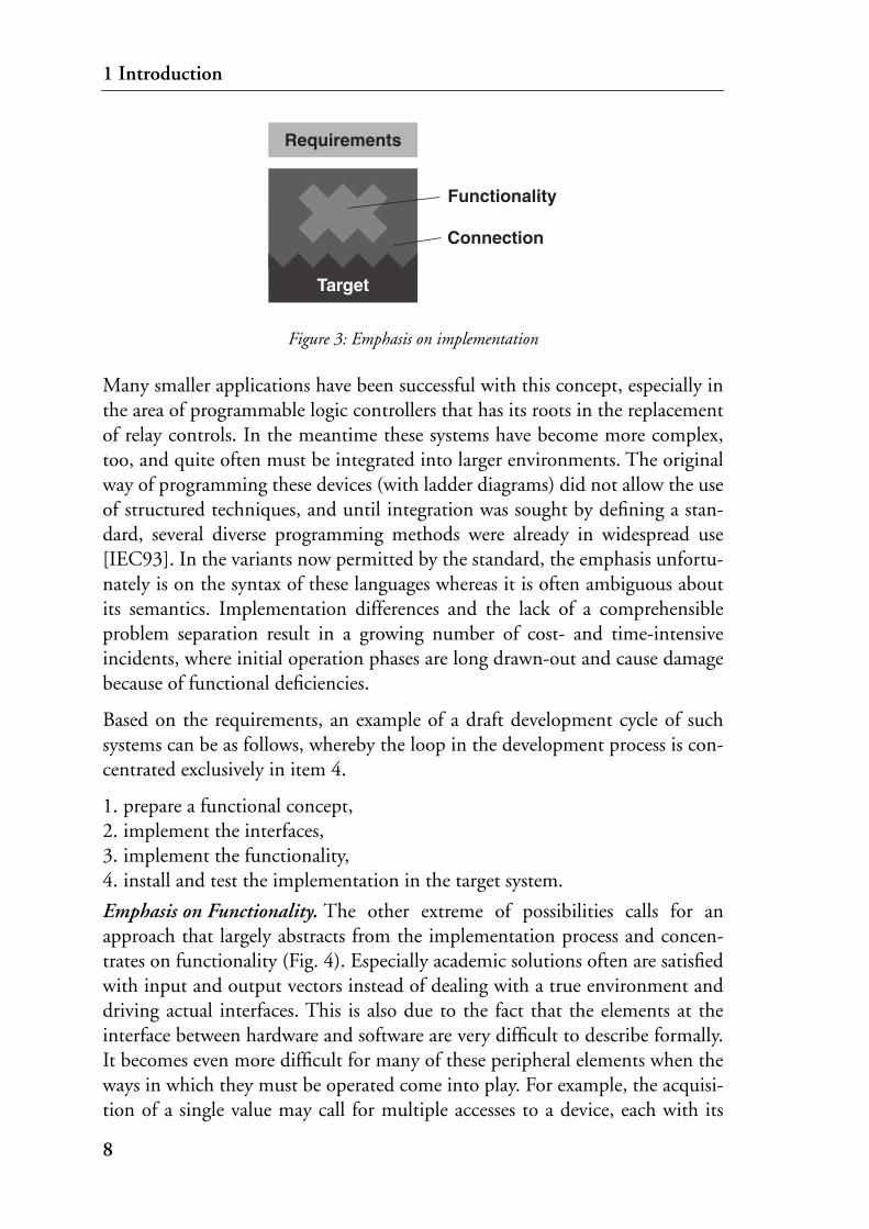
Emphasis on Implementation. If the emphasis is placed on the implementation(Fig. 3), hardware characteristics dictate how to proceed, at the same time pre-suming that functionality is the smaller problem. The concepts on which thisapproach is based often require a separation of different spheres, too, and thetask is approached accordingly. However, in the course of the development thelimits between the solution that is found and the way in which it is realizedbecome increasingly blurry. Often the original requirement specification disap-pears completely from the field of vision and thus is no longer of use duringsubsequent revisions.

Functionality

Connection

Requirements

Target

7

1 Introduction

Figure 3: Emphasis on implementation

Many smaller applications have been successful with this concept, especially inthe area of programmable logic controllers that has its roots in the replacementof relay controls. In the meantime these systems have become more complex,too, and quite often must be integrated into larger environments. The originalway of programming these devices (with ladder diagrams) did not allow the useof structured techniques, and until integration was sought by defining a stan-dard, several diverse programming methods were already in widespread use[IEC93]. In the variants now permitted by the standard, the emphasis unfortu-nately is on the syntax of these languages whereas it is often ambiguous aboutits semantics. Implementation differences and the lack of a comprehensibleproblem separation result in a growing number of cost- and time-intensiveincidents, where initial operation phases are long drawn-out and cause damagebecause of functional deficiencies.

Based on the requirements, an example of a draft development cycle of suchsystems can be as follows, whereby the loop in the development process is con-centrated exclusively in item 4.

1. prepare a functional concept,2. implement the interfaces,3. implement the functionality,4. install and test the implementation in the target system.

Emphasis on Functionality. The other extreme of possibilities calls for anapproach that largely abstracts from the implementation process and concen-trates on functionality (Fig. 4). Especially academic solutions often are satisfiedwith input and output vectors instead of dealing with a true environment anddriving actual interfaces. This is also due to the fact that the elements at theinterface between hardware and software are very difficult to describe formally.It becomes even more difficult for many of these peripheral elements when theways in which they must be operated come into play. For example, the acquisi-tion of a single value may call for multiple accesses to a device, each with its

Functionality

Connection

Target

Requirements

8

1.1 Development Concepts

own timing requirement, which in an implementation may suggest the use ofinterrupts. Hence it becomes clear that with regard to the overall task the envis-aged abstraction proves to be merely an incomplete description.

Figure 4: Emphasis on functionality

Since this approach pushes the development forward independently of thecomputer architecture and the peripheral devices for as long as possible, itresults in problems that become obvious only in the later phase of implementa-tion. For example, changing processor loads in the target system can have anegative impact on the response of controller algorithms or even cause instabil-ities in the control loops. In these cases, the goal may still be achieved withadditional resources in the form of more or faster hardware. This possibility,however, remains barred in developments for consumer goods where economyis of main concern.

In the following example of a draft cycle for an adequately complicated system,a process model is being used. It shows that not even successful testing with themodel protects from undesirable surprises when moving to the target system.

1. prepare a process model,2. simplify the model until it can be used for the control design,3. prepare the control structure,4. design the algorithms of the control and fine-tune them iteratively until they

seem acceptable when compared to the reduced model,5. test the algorithms with the help of the process model. This phase may result

in changes to the algorithms, the reduced model or even the process model,6. integrate the implementation into the target system and test the hardware

and software of the control system together with the environment.

This approach contains several development loops in items 4, 5 and 6, wherebyespecially the final step can be very cost- and labor-intensive. Oftentimes, seri-ous problems do not show up until tests are performed in the final installation;these can be simple coding errors, unexpected influences of the computer

Functionality

Connection

Target

Requirements

9

1 Introduction

structure on the dynamic response, or new findings in general that did not sur-face during the testing process with the model, since the models are usuallybased on deficient abstractions that may hide relevant properties. The imple-mentations in the testing environment and in the final system are very differentand thus are hard to compare anyhow. If, after some fine-tuning, it becomesnecessary to switch from the testing environment back to the model, thechange is likely defective and requires extensive manual adjustments. In practi-cal applications this step is hardly ever taken, so that the two types of imple-mentation increasingly diverge. Such a set-up can still provide valuable servicesduring the development phase since the participants are familiar with the sub-ject. However, in subsequent expansions the knowledge of existing analogieswill be lost, which is why the model will no longer be available for these pro-cesses either.

This technique has some other disadvantages. When determining the controlstructure in item 3, the assumption is that a top-down division of the overallproblem into independent parts is feasible. This also implies that changes to asingle module do not have any consequences for some other module. Theassumption often does not hold and this is one reason why true testing onlybegins after the system is completely coded. Anticipated changes in the imple-mentation have an effect on the entire structure and therefore are not onlyexpensive with regard to cost and labor as described, but they also endanger thestability of the entire design.

1.2 The ToolboxThere is no doubt that embedded systems are complex. If the methods andtools used in their development are also complicated, they accentuate the prob-lem instead of contributing to the solution. The wealth of the different ways insoftware development indicates that in software practically everything can beimplemented, sold, and even applied; the decades-old prophecies of an imme-diate collapse of the software technology have not yet come true. This maychange. Although it is probable that in consumer goods time to market andfeature count continue to be the driving forces, in other areas software correct-ness will become important (again?). This mainly concerns equipment that ispart of the infrastructure we rely on in our interactions with the environment:transportation, energy, health care, financial matters, etc. The growing propor-tion of software in these areas has been predicted to boost modeling tech-niques, code verification and analysis [JaR99]. The expectation is that thenumber of faults in embedded systems will decrease, once analysis of huge pro-

10

1.3 Overview

grams becomes feasible through progress in these techniques and the increasedperformance of future computers. All is not lost even before these wishesbecome reality, because, in addition to being a prerequisite of formal verifica-tion, models also serve another purpose. A model based on a formal foundationhelps in clarifying concepts through simplicity and uniformity, which is amajor contribution to keeping the number of possible mistakes at a minimum.Therefore, the presented approach is based on three simple principles:

• consistent separation of two spheres: functionality on the one hand, and its connection to the processes in the environment on the other hand,

• specification and modeling on a high level of abstraction; this concerns not only system behavior and response, but also the embedding into a hardware environment,

• replacement of manual coding through efficient, generated code with deter-ministic properties that can be statically analyzed; a prerequisite for lean solutions.

1.3 OverviewThis thesis presents nothing new. Most of the accommodated techniques havebeen known for decades. The aim was to offer a coherent solution for the per-ceived need of practitioners that incorporates and reconciles methods and toolsfor each development stage. In an attempt to separate the wheat from the chaffin today’s abundant propositions of how to tackle the different aspects of real-time systems, the emphasis has been on identifying a required minimum set ofsuch techniques. It is considered essential that a clear separation of concernscan be achieved, which encourages limitations of a tool’s power to what isneeded. Because these tools are closely related parts of a whole, their teamworkin mutual consideration assists in making implementations simpler and helpscut off a whole welter of consequences that otherwise must be dealt with. Fromthe point of view of the developers, the different aspects of a project presentthemselves on a high level of abstraction, whereas in the implementation thisapproach does away with dynamic scheduling, resource contention, priorityinversion, sporadic tasks, all of them objects of their own disciplines in com-puter science. At the same time it improves on the issues of predictability andefficient use of processor resources.

In chapter 2, embedded systems are presented in more detail and an attempt ismade to define minimum requirements, taking into consideration all the differ-ent aspects. These requirements lead to claims that must serve as guidelines

11

1 Introduction

when the combination of methods shall lead to efficient and lean solutions.The economic use of resources goes hand in hand with implementations thatare as small as possible, i.e., not cluttered with puffed-up additions not pertain-ing to the actual solution itself. During development, on the other hand, a highlevel of abstraction must be envisaged, with representations of the variousproblem areas in terms of the respective problem itself. All development phasesbenefit, if the principles applied in different problem areas are based on thesame grounds and share more than the syntax at an interface. Aside from intro-ducing different views on architecture, chapter 3 describes two kinds of prob-lem decomposition. One is concerned with layers of abstraction dividingspecifications and models from the implementation. The other one deals withthe separation of two fundamental concerns and a way to guarantee the interplayof the particular models. The correspondence does not only exist on a highabstraction layer, it is equally true for the code that is produced from suchmodels. Considerable advantages for the implementation result, if this codeconforms to certain restrictions instead of just being a collection of indepen-dently schedulable black boxes. The braces that hold these spheres together isthe pivot, the component architecture, which is presented in chapter 4, whereaschapters 5 and 6 are devoted to the methods used to tackle the problemswithin each sphere. Functionality is modeled in the graphic environment ofCIP Tool [CIP00]. Its expressive power is appropriate to what is needed inembedded system development, and the code produced by the tool is efficientand deterministic. The connection with a real hardware environment is achievedon an equally high level. Here, specifications are translated into code that com-plements the functional code. In chapter 7, the implementation is consideredfurther and the obtained code blocks and their calling conventions examined.The properties of this code are the prerequisite for implementations that excelin simplicity and have deterministic timing behavior. Appendices A and Bpresent the specification languages and tools used in the solution of the connec-tion problem.

Original contributions center on the architectural view, the connection prob-lem, and the implementation. All these aspects are dealt with on a high level ofabstraction, to this end specification languages were defined for the componentarchitecture, as well as for low-level data manipulation associated with inputand output. Code generators provide an automatic link from the high leveldescriptions to implementations. The implementations for their part benefitfrom the strictly controlled properties of the generated code. As a side-effect,worst case execution paths need not be extracted painfully from the final code,but are provided by the generators directly.

12

1.3 Overview

The claim of the presented approach is its usefulness in solving the entire prob-lem that the development of complex embedded systems presents. To demon-strate this capability it was put through its paces in a demanding application,namely the project Hybrid III. In chapters 8 and 9 its system structure andcontrol system is described at length. Hybrid III attempts to improve fuel effi-ciency and to reduce emissions of private vehicles in the entourage of the per-ceived need for less polluting traffic in the industrial capitals at the end of thefirst automotive century. The idea consists not so much in developing a com-pletely new kind of vehicle, but mainly in pushing the limits of current drivetechnology to the extremes. This project was the touchstone for many of theconcepts presented and it showed all the attributes of a real-world situation. Itstarted out with vague specifications that were changing continuously, itinvolved several institutions with many people from various fields and of differ-ent expertise. Control system technology had to stand back in view of the ‘real’problems the mechanical and electrical engineers were facing, they even choseto ignore it completely as long as it functioned correctly. It would have beeninadequate, to say the least, if the methods we proposed had only satisfied the-oretically. Project management, various operation modes with frequent changesfrom one to the other, and the coordination of many contributors, broughtabout additional hardships to the routine issues of a hard real-time system. Inthe end, a functional system had to be delivered. It has been our ambition toreach this goal as a side effect of a consistent development setup that emergesfrom a combination of selected methods, no hacking involved.

In an attempt to maintain the train of thought throughout the chapters, theexplanation of recurring, often-used terms is subsumed in a glossary.

13

1 Introduction

14

2 Embedded Systems

Fast technological advances in the field of hardware accompanied by decreasingcosts resulted in the current trend towards computer supported controls foralmost all industrial processes and many devices in daily life. These are elec-tronic systems that fulfill a limited number of predetermined tasks. Since thesetasks usually remain unchanged over the course of the entire life of a device,such systems cannot be programmed freely like, for example, a workstation.The applications differ widely and reach from radios and washing machines tosafety related tasks in airplanes and medical devices. Computers that are com-ponents of a larger system whose primary purpose is not computation, arecalled embedded systems; they control their environment and are connected toit via sensors and actuators [Kün87]. Aside from their much more specificapplication, the major difference to a workstation is indeed to be found in theenvironment. The environment of embedded systems is not intelligent and iscontrolled by the computer and not vice versa (Fig. 5). This is also the reasonwhy incorrect operation of an embedded system can have implications for thesafety of its users and their surroundings [Sto96]. Since the consequences offailure can be severe, these machines must behave correctly without interven-tion also in the presence of faults, which implies that they handle errors all bythemselves and recover from unexpected digressions.

Figure 5: Embedded system

Sensors

Actuators

Controlledprocesses

System tasksSchedulerCommunicatorClock…

Application tasks…

Embedded SystemEnvironment

15

2 Embedded Systems

Many embedded systems are reactive, i.e., in a continuous loop such a systemfirst tests a number of inputs for changes, then processes them to produce anumber of output values. These systems are integral parts of a feedback loopwith the external world. Embedded computers need not be small, or even allthat real-time, indicating that the terms ‘embedded’ and ‘real-time’ are inde-pendent of each other.

The processes in the environment are parallel and determined by physical,chemical or other principles that in turn depend on the respective application.Continuous information is translated to its discrete representation at the inter-face between environment and control system, and even time is represented bya discrete approximation. Since the peripheral hardware is able to convertmany input values simultaneously, there still is a high degree of parallelism atthis point. In most customary control applications, a single processor thenreads the data individually and processes them sequentially. Distributed controlsystems, on the other hand, work in parallel with several processing nodes. Thismakes it easier to adjust the required computer performance to the controlissue at hand and facilitates separate development. It also is advantageous withregard to maintenance and the reuse of components. Either way, conventionalsolutions contain quite a few parallel processes for which it is very difficult toguarantee that they cooperate smoothly, and that the timing requirements aremet under all conditions. Efficient strategies for cooperation and communica-tion within the system have a key role in these applications.

Often the calculations that a control system performs are time-critical. It is inthese cases that embedded computers are real-time systems with stipulatedresponse times to certain sensor signals. The reactions must not only be func-tionally correct, but they must happen at the correct time if such a requirementis postulated (temporal correctness). The scale of the desired real-time responsevaries very much and can range from seconds to µs. Hard real-time cases aremarked by a specification of a maximum response time that must never beexceeded. Soft real-time, on the other hand, allows for a defined statistical dis-tribution of response times for each and every action, always at some requiredheavy level of processor activity. Timing requirements are quantifiable andmeasurable, and they either are postulated directly as part of a system’s specifi-cation, or they may emerge as a consequence of other stipulations. For exam-ple, the desired positioning speed and accuracy of a machine tool dictates theminimal sampling rate for the measured quantity ‘position’. Aside from satisfy-ing timing requirements, which is mandatory in hard real-time systems, it isalso desirable to obtain a high utilization of the resources that are present in aninstallation. If a high production volume is planned, reducing the indispens-able resources to a minimum may become a distinctive requirement in itself.

16

2.1 Requirements

Currently, developers often seem to be satisfied with any feasible result that ful-fills these requirements, although it would be possible and preferable to findoptimal solutions for both the timing and performance demands. Thisbecomes possible when all related elements have deterministic behavior thatcan be analyzed in advance [XuP93]. Fortunately, hard real-time requirementsusually are restricted to parts of a system, which in turn helps to achieve accept-able computer utilization. As outlined, failures in real-time systems do not nec-essarily imply incorrect results from computation, they also refer to (andpresently more often) violations of temporal requirements. Attempts tocounter this type of failure involve generous hardware resources that reduce theaverage performance of real-time systems compared to that of non-real-timesystems. This implies that a system cannot be chosen on the basis of its averageperformance, if latency or worst case performance is the key issue.

Work on embedded systems is characterized by cross-development, i.e., themachine where the development takes place is not identical with the final tar-get. The advantages offered by a powerful workstation environment withsophisticated tools and network facilities for cooperation in a team are out-weighed by the difficulty of gaining access to programs and data once they areinstalled and running in their targets. This is notably true in the case of distrib-uted systems, which are virtually impossible to observe and debug during oper-ation [Dan97].

2.1 RequirementsThe one advantage in the development of embedded systems is that the charac-teristics of the application and its operating environment are more preciselyknown than that of general purpose machines. Using this information, it ispossible to fine-tune real-time systems accurately for optimum performance.

Aside from the requirements raised by a client specification that describes whata system should do once it reaches completion, an additional collection of vari-ous requirements is stipulated by the characteristics of a real-time system’s prin-cipal constituents (Fig. 5). Most of the demands are dictated by the processesin the environment and they also depend on how external information is con-ditioned for use by the digital embedded system. This system itself consists of apossibly large number of processors, equipped with local resources for comput-ing and storing data, and interconnected by a real-time communication net-work that provides bounded communication delays. The real-time operatingsystems that manage the use of processors and resources range from simpleexecutives to complicated aggregates that handle preemptable tasks and resolve

17

2 Embedded Systems

arising conflicts in resource usage. Performance must be traded for reliability infault tolerant systems that require additional management of redundant hard-ware and software components.

There are two fundamentally different paradigms that are referred to in thecharacterization of real-time systems. In event-triggered real-time systems, anysystem activity is initiated in response to the occurrence of a particular event inthe system environment, whereas in time-triggered systems, activities are initi-ated at predefined instants of the globally synchronized time [PaD93]. It is acommon misconception that the paradigm best suited to describe one specificview of a system (usually the implementation) must extend to the whole andinclude all the different viewpoints from the abstract model to the target imple-mentation. In fact, the best way of dealing with functionality on a high level ofabstraction is in stark contrast with how this functionality should be imple-mented, especially in cases where predictable behavior must be guaranteed.Because in the event-triggered approach the expiration of time can be treated asa sequence of time events, and in time-triggered systems discrete events aremerely deferred by some predefined amount of time, the two ways of dealingwith the problem are really equivalent. This is why there is a choice of the dif-ferent representations for each level of abstraction.

The following compilation attempts to highlight the essential requirementsand to draw up a number of claims that are raised against any suggestions ofhow integral embedded system development should look like. Somewhat con-tradicting demands are inevitable, hence there is no way to a solution withoutcompromise. Nevertheless, these guidelines provide valuable assistance in dis-criminating essential properties from those that can be more easily sacrificed.

2.1.1 Functional Requirements

The objects in the environment exhibit a specific behavior according to theirphysical, chemical etc. properties and their interdependencies. It is the goal of acontrol system to bring about specific interactions between these objects. Thisinteraction can be realized by means of the reactive behavior of a computerprogram, in an analogous way that it could be achieved pneumatically ormechanically. The essence of a customer’s requirements is just what this behav-ior should be. Unfortunately, and for a variety of reasons, the conceptionsavailable at this stage are incomplete, often contradictory and do not provideenough detail to serve as a basis for further reasoning [LCF97]. In order to beable to continue from here, a new comprehensive picture of the system to bebuilt must be created using a notation that permits the customer to understand

18

2.1 Requirements

what it is about and which can at the same time serve as a foundation of furtherprogress. The means by which a system’s functionality is described must there-fore be based on some kind of formal model, using textual and graphic repre-sentations for defining systems, processes, their behavior, and theirinterrelations. Notations exist in many different variations: formal descriptionlanguages that were created for use in a special application domain (such asSDL for the telecommunications industry), state-based notations especiallysuited for reactive systems (of which Statecharts is a prominent, but unfortu-nately only partially formal example), or strictly formal languages, which areapplied when the emphasis is on formal verification (such as Petri Nets, VDMor Z). In any case, it would be most desirable that a high level description ori-ents itself along the lines of the informal requirements. These come in a varietyof representations including graphs, pseudocode snippets and natural language.Hardly ever do they coincide with the structures of formal models such as PetriNets or algorithmic languages, instead they very often already show the charac-teristics of automata with a finite number of states.

What is the most suitable paradigm for these representations? On the onehand, the internal behavior of embedded systems, where any change of state inthe environment calls for a reaction, makes them a perfect match for the event-driven model, on the other hand, an increasing number of these systems incor-porate control loops that require periodic execution irrespective of the courseof events in the environment. These parts of a system suggest the application ofthe time-triggered paradigm, but, because the reaction to asynchronous eventspresents the most demanding functional issue, it seems appropriate to choose adescription based on events for the entire problem area. The passing of time isthen treated the same as all the other (sporadic) events originating in the envi-ronment.

Claim 1: The problem at hand must have a comprehensive representation at a high level of abstraction. This representation must accompany the system and its developers through all development stages and allow for seamless transitions into implementations. The number of additional precondi-tions imposed on the implementation must be minimal.

2.1.2 Temporal Requirements

Temporal requirements are raised by the properties of the real-time processes inthe environment. A distinction has to be made between two different kinds oftemporal demands. One is concerned with the amount of time that is allowedto elapse until the system reacts to a discrete event in the environment. The

19

2 Embedded Systems

other kind of temporal requirement is associated with external processes thatare part of periodically executing control loops. Examples of the first type, whichmay require either hard or soft real-time response, are the reactions to the pushof a button, or to the event of a continuous signal exceeding some predefinedlimit. Hard real-time response is indispensable for the cyclical execution ofcontrol algorithms that belong to the second category. In addition to the usualmaximum reaction time, an upper bound on input jitter is imposed for controlloops. In absolute numbers, the spectrum ranges from man-machine interfaceswith modest calls for maximum response times in the range of 40 ms (instanta-neous for a human observer), to the demanding control loops in solid stateswitching for electrical drive applications, which are among the fastest withinthe realm of today’s control systems. For digital signal processing, continuoussignals must be quantized at some discrete interval after which they appear tothe computer as a sequence of digital values, i.e., values that are limited to dis-crete steps in amplitude. This quantization adds random noise to the signalwith a uniform distribution among , LSB being the least significantbit, corresponding to the distance between adjacent quantization levels.

The time interval and the accuracy (or resolution) of this transition must bechosen according to the properties of the controlled process, with shorter peri-ods resulting in better closed loop characteristics. Within limits it is possible,however, to vary the sampling time and adapt the control laws such that thecharacteristics remain acceptable. As a rule of thumb, sampling intervals for asignal must amount to approximately th the process’ characteristic timeconstant in Fig. 6 [Kop97, Unb87].

Figure 6: Process step response

1 2⁄ LSB+−

1 10⁄drise

td object d rise

10%

90%

20

2.1 Requirements

Sampling. Together with quantization, digital signal processing dependsheavily on sampling. The signals in the environment evolving continuously intime must be represented by just a set of their values. According to the sam-pling theorem, the sampling rate must be greater than twice the signal’s highestfrequency component, if the properties of the signal shall remain unalteredthrough this process [Cat69]. Data under observation must be band-limited toa frequency less than a critical frequency, otherwise aliasing and severe nonlin-ear distortion result. Because the sampling rates are chosen in accordance withthe interesting part of a signal’s spectrum, low-pass filters (aptly called anti-aliasing filters) must be used on the analog side of the conversion to precondi-tion the input signal [Smi97].

In practical applications, the characteristics of the available non-ideal filtersintroduce selective attenuation and phase shifts (Fig. 7). Therefore, finding fea-sible combinations of sampling rates and filter characteristics involves a trade-off between filter complexity and sampling speed, and it always results in theneed of higher sampling rates than postulated by the sampling theorem. Theeffect of using too low a sampling interval in closed loop control is first anincrease in settling time and in extreme cases instability.

Figure 7: Filter magnitude and phase vs. frequency response

Jitter. Implementations of control algorithms have an additional temporalrequirement. It is not caused by the processes in the environment, but rather bythe way continuous information is fed into the digital system. When discretecontrol algorithms are based on a fixed sampling rate for data capture, and thisfrequency is subject to jitter (which may be caused by scheduling issues, orinterfering interrupts), these algorithms may suffer from stability problems.The reason is that input signals experience a measuring error proportional tothe temporal variation of the instants when the samples are taken (Fig. 8).Especially signals with a steep gradient introduce disturbing excursions of the

Φ

Passband

A max

Transitionband

Stopband

A min

dB

ff

21

2 Embedded Systems

read values that may eventually cause the control algorithm to fail. The worstcase occurs when a signal is sampled alternatively at the beginning and at theend of the sampling period.

Figure 8: Jitter effects

The majority of currently proposed implementation techniques build on taskscheduling schemes that are based on priorities with exclusion and precedenceconstraints only. Such implementations leave the extent of jitter undefined.This situation is aggravated in systems that rely on the use of hardware inter-rupts to capture sporadic events. The consequence is that control engineerstend to push the sampling rates in their requirements, so they can use filters toeliminate jitter effects from a signal. Unfortunately, additional filtering intro-duces longer time delays into the control loop, and, if a system contains manysuch signals that are actually oversampled, the total work load rises unnecessar-ily. This in turn may induce additional scheduling problems that will causeeven more jitter. Even if the variance in input sampling rate is small, jitter canbe present on the output signals, which is caused by delays in processing, orbecause signals are buffered before they are written to their respective devices.Usually, this is not a problem, since actuators and their connected machineparts can tolerate some jitter without adverse effects. Furthermore, jitter mayalso be introduced when deadlines must be sacrificed for some other moreimportant issue. For example, in a radar system it is crucial to avoid data losseven at the expense of missed deadlines. By using buffers between the radarhardware interface and the subsequent processes the latter can be preempted,so no data is lost. Instead, the arrival time of processed data will gain some jit-ter. A system with multiple dedicated processors is very effective in reducingthis kind of jitter.

Claim 2: Sampling intervals for periodic closed-loop control tasks must match the ones postulated by the problem analysis based on control theory. Input jitter for these signals must be kept minimal, and its amount must be controllable and guaranteed.

t

∆V

V

∆d

∆V = dV(t)dt

∆d

22

2.1 Requirements

Soft Real-Time. In contrast to hard real-time requirements, where it must beensured that all deadlines are met, there are some choices in soft real-time.

One possibility is to handle these requirements no different from those for hardreal-time, a frequent option when the resources present in a system surpass thesummed up requirements. If this is not the case, processing time that is avail-able to those parts of a system with soft real-time requirements must be parti-tioned according to functional properties of these tasks. Different policies maybe appropriate: possible failures to meet a deadline can be taken into accountby stopping a task and handing the processor over to another one. Or, forexample, in a video conferencing system, the last frame is kept when the datafor the next frame has not arrived by the expected deadline. An interesting pos-sibility in soft real-time are algorithms that are inherently soft, i.e., algorithmsthat lead to increasingly better results over time. Examples for this kind ofapproach can be found in vision decision systems. There, computation contin-ues, with possibly different algorithms, until the deadline arrives. Thisapproach requires at least one (the simplest) algorithm to have a hard deadline.It must be noted that picking a strategy that is adapted to a specific problemcan be more challenging than determining which parts of a system must bedesigned to meet which deadlines.

Figure 9: Variations in processor resource allocation

Although embedded systems with only soft real-time requirements do exist, inthe case of hard real-time requirements this is hardly ever true for entire sys-tems. There, hard and soft real-time requirements appear side by side and facil-itate optimal resource utilization even when the processor loads generated byhard real-time tasks vary greatly. Thus, when hard real-time demands decrease,resulting from a change in system behavior such as shown in Fig. 9, the freedcapacity will simply be allotted to pending soft real-time tasks. This, however,is only possible when the tasks with soft real-time requirements are fully pre-emptable, i.e., it must be possible to interrupt them at any time without

0

20

40

60

80

100Soft real-time tasks

%

PeriodHard real-time tasks

23

2 Embedded Systems

adverse effects on the schedules of hard real-time tasks and the availability ofresources needed by them.

Claim 3: Tasks with soft real-time requirements must be preemptable, and their use of global resources must be limited to issuing requests through buffer-ing mechanisms.

2.1.3 Accuracy Requirements

Input and output values in embedded systems are characterized by having afixed range, which is determined by the physical process and the technologyused in specific sensors and actuators. The values within this range areexpressed with a finite resolution, determined by their binary representationand by the mechanism employed when converting from analog to digital orvice versa. One stage in the chain of involved elements decides on a signal’s res-olution. Very often (as in the example in Fig. 10) the severest restriction isbrought about by the accuracy of the sensor itself, which is easily surpassed bythe accuracy of an integer representation within the control system. From thepoint of view of resource adequacy the optimum would be to choose matchingrepresentations on all stages involved. This rules out floating point in manycases, although a direct conversion to this format may be preferable in systemswhere a floating-point unit is present and used to perform calculations.

Figure 10: Input signal range and resolution

Absolute accuracy requirements are often rather lax for various reasons. Valueinaccuracy frequently is not brought up by the ways data is handled in digitalsystems, but it is inherent in the physical processes themselves. The presence ofripples and other disturbances in a tank, for example, makes it pointless tomeasure its filling level with meticulous accuracy. In another context, measured

Process

Range ResolutionStage

10…120 °C continuous

4…20 mA2…10 V

0.5 °C ≈ ±0.6 %

205…1023

10 bit ≈ ±0.2 %

-3641…32767

signed int ≈ ±0.003 %

-20…180 °CSensor

A/D-Converter

Unit conversion

24

2.1 Requirements

values may have chiefly relative significance, particularly the ones used in con-trol loops. The reason is that a controlled process can only be stabilized withappropriate measurement repeatability, whereas the actual accuracy of thesemeasurements is of secondary importance.

Claim 4: The accuracy of signals and their representation must be adapted to the chain of elements from a process’ physical properties to the data formats required by the control system.

2.1.4 Implementation Requirements

Implementation requirements depend on the characteristics of the hardwareenvironment, as well as on the paradigm that forms the basis of a specificimplementation, which as described is either event-triggered or time-triggered.Both strategies require a resource management that guarantees the availabilityof the resources needed by a task, prior to the execution of that task. In bothapproaches the resource needs and availability assessment must be carried outwhile taking into account the timing requirements of the applications. Becausein event-triggered systems the resource needs and their availability may vary atrun time, resource management becomes dynamic and hence much more diffi-cult. On top of that, timeliness guarantees may be violated in case the assumedpeak load is exceeded during run time. Time-triggered systems benefit from atimeline divided into regular intervals, which allows for an off-line computa-tion of resource needs. These needs are based on estimation, code analysis, orexecution time measurement prior to deployment. Furthermore, time-trig-gered systems do not face the excessive number of possible behaviors, which inevent-triggered variants must be carefully analyzed in order to establish theirpredictability [Jos96]. In comparison, event-triggered solutions are more flexi-ble and less prone to waste resources.

While the choice of a paradigm for the implementation is often tightly linkedto the paradigm chosen for the functionality, it is important to note that this isnot necessarily so (as described in 2.1.1). On the contrary, the right choices inthese two spheres may be exactly opposed, and it is not a problem to incorpo-rate functionality based on an event-triggered model in a time-triggered imple-mentation. These implementations are easier to master and the code’scompliance with timing requirements on specific targets can be checked beforeinstallation.

Implementation efficiency is another important factor in embedded systems.The necessity of efficient coding to make optimal use of processor resourcesand to find one’s way in tight memory occupation is one reason why program-

25

2 Embedded Systems

ming in assembly language is still widely used. This is especially so in areaswhere small systems and large numbers of installations are envisaged and thegoal is to make do with minimum hardware.

On the other hand, the enormous performance increase of today’s processors inthe field of complex applications has resulted in the use of elaborate real-timeoperating systems. Their enticing ability to deal with a great number of tasksand to manage resources dynamically has not failed to show its influence oncontemporary systems. The requirement to provide binding information onthe system response and its ways of interaction has given way to techniquesthat can provide estimates at best. This is quite astonishing in light of theinvolved risks to humans and material values [Lio96, Risks].

Claim 5: The resource requirements and the timing behavior of the final imple-mentation must be open to exhaustive static analysis. System perfor-mance should match the requirements, hence permit optimum resource usage.

2.1.5 Communication Requirements

On a higher level of abstraction the term communication is extremely compre-hensive and includes a plethora of ways of how different entities can interact. Acommunications infrastructure must be capable of supporting both signallingfor transactional interchanges and data propagation. Basically, all these meth-ods are either synchronous or asynchronous. In many approaches the imple-mentation of these interactions is abstracted away and it is assumed that somekind of agent between the various nodes in a distributed system will providethe required mechanisms (for example CORBA, which does not require thedefinition of task locations until run time [OMG95]). This view neglects thattiming constraints may be associated with communication, with varyingrequirements depending on where specific connections within a layered systemare situated. At each level the performance must fit the requirements of thecommunicating elements, which are typically more stringent the lower thelevel is.

On the level of implementations, the most simple case of communication isthrough global data, where a flag signals the receiving task that data is available.It is up to the receiver to check for any data that it may receive and to reset theflag after reading the data. Synchronous behavior of different tasks is accom-plished easily, but this scheme obviously only works for communication thatdoes not leave the common memory boundary of both tasks involved. If sev-eral nodes with their own processors and particular memory are involved, i.e.,

26

2.1 Requirements

if basically asynchronous entities need to communicate, a communication net-work with appropriate protocols must be used. Networks range from wide areamultimedia services to local instrumentation networks. They are related in thatthey demand a predictable quality of service, but differ considerably in thenature of their requirements. In a non-interactive television broadcast, forexample, a high bandwidth and bounds on jitter are postulated, whereas delayis not critical. In playback applications, these criteria are the quality of serviceparameters that need to be controlled. If the bandwidth is not sufficient, pack-ets are dropped as soon as the queuing capacity is exhausted. Also, the availablebandwidth must exceed what is needed by the average transmission rate, sobursts can be cleared quickly. This differs from an instrumentation networkthat periodically transmits time-critical sensor data, where bandwidth may bemarginal, but upper bounds on delay are essential.

Communication mechanisms that fulfill different needs can be classified asbelonging to a generic type of communication network, two of which mustprovide guaranteed temporal performance (Fig. 11). At the lowest level, theinstrumentation network connects a real-time system with its sensors and actua-tors. The requirements regarding latency and jitter are high, but because itsbulk load consists of mostly small data packages, which are transmitted period-ically, efficient and economical solutions are possible. The real-time network isthe means of communication of individual nodes in a distributed real-time sys-tem. Here, deterministic behavior is most important, whereas demands onlatency and jitter can be traded for reliability and fault tolerance. Operationalrobustness requires that correctable transient errors must not impair servicepredictability. Throughput should increase monotonically with the load andthrashing must be avoided. Finally, the backbone network links a real-time sys-tem with other systems [ARS91]. No hard real-time demands are imposed onthese connections, and they are therefore not considered any further.

Figure 11: Embedded system communication architecture

Communication node

I/O node

Working node

Actuators

Sensors

…

Backbone network

Real-time network

Instrumentation network

…

…

…

…

27

2 Embedded Systems

Another classification is concerned with traffic volume and message sizes in dis-tributed embedded systems. Some applications, for example in vision and radarsystems, rely on high-volume data distribution. These messages must be dealtwith alongside the more common communication traffic consisting of short,periodic messages. Networks for different applications therefore must vary sig-nificantly in their distinctive features. To choose the simplest network technol-ogy fulfilling the requirements is worthwhile not only because of costconsiderations, but also because a complex protocol constrains design anddevelopment flexibility. Using available resources efficiently becomes difficultwhen an application must incorporate communication black boxes with a col-lection of services not needed for that particular installation.

The interplay of partners communicating in a distributed system may be gov-erned by higher level protocols, but it is the media access protocol that deter-mines a network’s performance: efficiency, determinism, robustness, andflexibility. Efficiency denotes the relation of transmitted message content to rawnetwork bandwidth, which is lowered by additional information in each mes-sage, and by the arbitration mechanism used to gain access to the network.Thus, for some protocols, the efficiency may vary greatly with network load,which in turn affects worst case behavior. Deterministic latency, or boundedand predictable message delay, can be achieved only under light load condi-tions with certain protocols, whereas it is inherent in others. Operationalrobustness depends on a protocol’s ability to quickly detect and recover fromtransient errors. Furthermore, if a serious error occurs, all participating nodesmust be notified with a low latency. Finally, flexible protocols tolerate networkchanges without reconfiguration when nodes are added and deleted.

Claim 6: A real-time network must be predictable and behave deterministically. Although message size and other operational properties must meet the needs of the application at hand, network performance should roughly correspond with the required minimum.

2.1.6 Reliability Requirements

Reliability requirements also embrace safety, maintainability and availability.Reliability denotes the probability that a system functions correctly accordingto specifications over a certain period. Safety refers to reliability with regard tocritical failures that may have a harmful impact on lives and material. Usuallycost or statutory regulations or both are brought in as a justification for theadditional expenditures in developing safety-critical systems. Even in systemswith a high production volume that seem mostly driven by cost, reliability

28

2.1 Requirements

requirements may be high, such as in automotive applications that must oper-ate reliably over a typical lifetime of some 3000 driving hours. Furthermore, inthe long term, it may be expected that generally the tolerance for faulty pro-grams will decline in the same manner as the tolerance for collapsing bridgeshad declined. Therefore, the expectations of system reliability will eventuallyslop over to noncritical applications, which means that the quality status of allsystems must rise and that the development methods must concord with theseexpectations. Currently there remains a wide gap between ‘normal’ systems andsafety-critical systems, because reliability concerns cannot be integrated wellinto the development process. Therefore, this additional burden is left behind,unless enforced by necessity or by regulations.

There are two aspects to reliability that tend to be confused, especially in soft-ware engineering. One denotes the probability of faults caused by physicalbreakdown of a device or its constituents, an area of research and practice withproven methods used in assessing the reliability of all kinds of technical systems[Bir97]. Thereby a system’s failure rate is calculated on the basis of standardfailure rate models of its components. In a reasonably well constructed system asingle fault will not induce an unsafe condition, and the system may even beexpected to recover from transient faults. These, of course, may occur any timein both hardware and software. It remains another question if software shouldbe designed to handle all these cases explicitly, or if it may rely on exceptionhandling built for example into a language or operating system.

The other aspect is concerned with faults that are actually introduced intotechnical systems through inadequacies in the process of its design and imple-mentation. If engineers in one of the established disciplines are confrontedwith the latter, in all likelihood the incident concerns liabilities and guarantees,and it will attract lawyers. Unfortunately, systems that contain software areguaranteed to contain inadequacies, even errors, in their design. Therefore, insafety critical applications measures must be taken against both of these prob-lems, and in practice faults of both kinds very often get treated the same. Vari-ous models of fault tolerant system architectures have been proposed and putto use, including redundant systems featuring cold standbys, warm standbys,replication with self-checking, replication with voting, and various levels ofduplication [Sto96]. On the level of programs, a software architecture and lan-guage subset is selected that adds to the complexity of the problem at hand aslittle as possible. Likewise, systems can in a way be made insensitive to externalevents by choosing a time triggered approach. Time offsets are used to controlprecedence relations and to control jitter and drift, which also presents virtuallythe only way to achieve predictable behavior in distributed systems.

29

2 Embedded Systems

Some of these techniques, including the use of redundant hardware, are expen-sive, and they augment the complexity of a system. While cost considerationslimit their application to the area of safety-critical systems, the same reliabilityrequirement would call for simple solutions, which are easier to oversee, imple-ment and maintain. Those measures necessary to compensate for the additionalcomplexity augment costs even further. The cost-neutral measures, on theother hand, could be put to use profitably in all embedded systems.

Claim 7: Reliable solutions are lean solutions.

2.2 DevelopmentEmbedded systems differ from conventional data processing installations inmany ways. A major difference lies in their heterogeneous architecture, consist-ing of microcontrollers, dedicated signal processors, memories, and custom-built analog and digital components. As described in 2.1, they are characterizedby reactive behavior, real-time requirements, fault tolerance and predictability.The complex relationship between the involved hardware and software compo-nents, as well as the relationship of these components with a physical environ-ment make development of embedded systems difficult. The admonition to‘never trust an actuator’ leads to defensive strategies, which further complicatedevelopment work.

Additional problems arise from inevitable conflicts among constraints andoptimizing goals, and all this is made worse by the development process itself.It is characterized by a collection of methods that very often are only badlyintegrated into the development flow. The limitations and restrictions inherentin these methods and the tools they are associated with impair a developer’sfreedom of movement even further.

Cross-development, where the development platform differs from the intendedtarget, presents advantages with regard to available tools and network connec-tions with other team members and data bases. These advantages are out-weighed by difficulties encountered when attempting actual implementations.Because analytic methods – if considered at all – cannot master the complexityof real-world systems, this step is taken with incomplete and unproven solu-tions. To this are added the problems of debugging fast responsive and distrib-uted systems in operation. Therefore, the dominant problem in thedevelopment process is the wide gap that remains between the test phase in asimulation and the actual realization on the final target. This gap has beenapparent to many practitioners and is also slowly getting attention from aca-demic researchers, as illustrated in Fig. 12 (adapted from [ABB93]).

30

2.2 Development

Figure 12: Gap in the development process

The gap is narrowed with the application of design principles and methodsthat are aimed at precisely defined areas of the entire problem. It is further nar-rowed when these areas overlap only minimally, but it will not disappear aslong as the integration of different methods remains inadequate. Subsequently,various methods and techniques used in the development of embedded systemsare briefly presented. In the same manner as has been attempted for therequirements (see section 2.1), the central points of these methods are retained.

2.2.1 Building Principles

Two building principles are central to most established engineering disciplines.These principles – the pairs decomposition ↔ composition, or top-down ↔bottom-up – are associated with specific phases in a development process andcomplement each other ideally. Consider the building of a house, for example.It starts out with a planning phase, where an abstract view of the involved ele-ments and their interplay is sought. The final product of this top-down activityare blueprints that will be used in the later construction of the building. Thesubsequent construction is based on the blueprints, but is attempted with com-pletely different methods. It can be seen as the bottom-up composition ofsmaller constituents in such a way that elements with the properties and thecomportment as defined in the plans are obtained, a proceeding that stands outagainst pure top-down approaches relying on step-wise refinement. These existonly in software engineering, since in the example of building a house theywould lead to the reinvention of windows, doors, doorknobs, hinges etc. forevery new house being built. Architecture and design are top-down activities inboth cases, whereas the construction of the required elements is more favored

processmodeling

modelreduction

algorithmdesign

test insimulation

practicalrealization

31

2 Embedded Systems

by compositional, i.e., bottom-up approaches. One reason for this is thatassumptions about the top level of unknown systems should not be made at anearly design stage. Also, components obtained by decomposing entire systemsare not generic, which makes them hard to reuse.

It must also be noted that building principles are predetermined by the chosendevelopment method. Developers may be forced into adopting one or theother principle exclusively, or – even worse – they may be faced with an inscru-table conglomerate of both methods. This is the case with object-orientedmethods, where inheritance can be used not only to express specialization, butalso generalization. Therefore locality is lost, and the use of multiple inherit-ance especially leads to web-like dependencies.

Essence 1: Top-down decomposition and bottom-up composition complement each other. Both these principles are used to advantage in the respective application domains of architecture and construction.

2.2.2 Architecture

Even if the development approaches presented in section 1.1.2 lack an overallview, there is of course something to both of them. In fact, if an attempt oftackling the problem as a whole is to be successful, both have to be consideredcarefully. Therefore, in a well-balanced approach these extreme views ought tobe reconciled. In such an attempt, the starting point remains unaltered: looselycoupled spheres must be identified and isolated, so they can be dealt with sepa-rately throughout most of the development process. It is important to note thatpostulating the separation at the outset of the endeavour is not sufficient, nor isthe proposal of methods with which to attack the then separated problems ontheir own. The key issue is to go beyond the diverse spheres and the particularmethods used within a sphere, and enforce this isolation using a description ofthe components and their interrelation on an even higher level. In this bindingarchitectural view the points of contact between components are based on rep-licas of the associated elements that are present on both sides of the dividingline. Explicitly specified connectors between such components further assist inthe decomposition of entire systems [Sha96]. The component architectureoffers insights into a system’s structure on a high level and at the same timeensures compatibility of the low-level interfaces that emerge when code is gen-erated. It is the pivot of constructive development effort and the basis of projectconsistency; therefore it must be defined as early as possible. From then on, ifchanges are kept well under control, mutual influence of spheres that are other-wise but weakly coupled is effectively limited.

32

2.2 Development

This notion of architecture, which primarily deals with a system’s operationalstructure, is complemented by another view, commonly also termed ‘architec-ture’. This view is the implementation architecture that describes the hardwaretopology the system will be deployed on. Such a topology consists of a set ofresource items including processors, busses, sensors and actuators. Compo-nents of the abstract operational architecture must eventually be mapped ontoone distinct implementation architecture. Different approaches to architecturestreat these two aspects with varying emphasis, some of them reasoning aboutthe cooperation of components [AlG97], others focusing on the implementa-tion [GSH97, Kop97]. If architectural concepts are solely based on the level ofimplementation, they cannot be used to contemplate component interaction;on the other hand, if they neglect implementation issues in favor of abstractinteraction issues, they will not be of much use in practical development work[Mik99].

It is general industrial practice to choose the hardware environment at the out-set of a project, with the disadvantage that it will be evaluated only late in thedevelopment process, namely when the entire code is ready for installation. It ismuch more desirable to deal with an abstract operational architecture duringdevelopment and to postpone mapping this architecture onto real hardware aslong as possible. Such a generic component architecture does not only permitan optimum adaptation of hardware resources to the actual needs, it will alsotolerate changes in the implementation architecture due to unavailability ofkey hardware items, or due to a mid-life update of control systems.

Figure 13: Component architecture mapped onto different implementation architectures

A sample of these different views is given in Fig. 13. The operational architec-ture of this system consists in a decomposition into four components (top leftin Fig. 13). These components are mapped onto different implementationarchitectures with one to four processors. The example illustrates that systemdecomposition is only possible within the constraints of a given componentarchitecture, i.e., mapping onto more than four nodes would require a redesign

C

P OI

Processor

321

4

I Input

P Processing

O Output

C Communication

Component

unidirectional

bidirectional

Connector

33

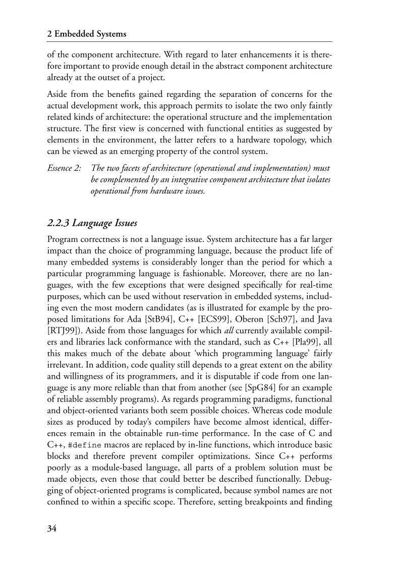
2 Embedded Systems

of the component architecture. With regard to later enhancements it is there-fore important to provide enough detail in the abstract component architecturealready at the outset of a project.

Aside from the benefits gained regarding the separation of concerns for theactual development work, this approach permits to isolate the two only faintlyrelated kinds of architecture: the operational structure and the implementationstructure. The first view is concerned with functional entities as suggested byelements in the environment, the latter refers to a hardware topology, whichcan be viewed as an emerging property of the control system.

Essence 2: The two facets of architecture (operational and implementation) must be complemented by an integrative component architecture that isolates operational from hardware issues.

2.2.3 Language Issues

Program correctness is not a language issue. System architecture has a far largerimpact than the choice of programming language, because the product life ofmany embedded systems is considerably longer than the period for which aparticular programming language is fashionable. Moreover, there are no lan-guages, with the few exceptions that were designed specifically for real-timepurposes, which can be used without reservation in embedded systems, includ-ing even the most modern candidates (as is illustrated for example by the pro-posed limitations for Ada [StB94], C++ [ECS99], Oberon [Sch97], and Java[RTJ99]). Aside from those languages for which all currently available compil-ers and libraries lack conformance with the standard, such as C++ [Pla99], allthis makes much of the debate about ‘which programming language’ fairlyirrelevant. In addition, code quality still depends to a great extent on the abilityand willingness of its programmers, and it is disputable if code from one lan-guage is any more reliable than that from another (see [SpG84] for an exampleof reliable assembly programs). As regards programming paradigms, functionaland object-oriented variants both seem possible choices. Whereas code modulesizes as produced by today’s compilers have become almost identical, differ-ences remain in the obtainable run-time performance. In the case of C andC++, #define macros are replaced by in-line functions, which introduce basicblocks and therefore prevent compiler optimizations. Since C++ performspoorly as a module-based language, all parts of a problem solution must bemade objects, even those that could better be described functionally. Debug-ging of object-oriented programs is complicated, because symbol names are notconfined to within a specific scope. Therefore, setting breakpoints and finding

34

2.2 Development

global variables becomes difficult without good naming standards. Finally,details left unspecified by the language designers, together with other detailsthat are too hard to implement, make C++ a non-portable language.

When code is generated instead of written by hand, the abstraction level of thiscode is a matter of choice. Much has been said in the favor of well-constructedand strongly typed languages that appear and vanish in various disguises. Gen-erated code in one of these languages has the advantage of still being compre-hensible, which may be an issue when source-level debugging is attempted (italso offers the questionable opportunity of manual modifications). The otherextreme would be to make code generators produce object code directly. Thefirst choice seems appropriate, but since many of the required assertions pro-vided by compilers for real high level languages can be performed by the codegenerator, strong typing, the absence of pointers, checking of array bounds andmany more are not compulsory for the generated language itself. On the otherhand, the use of assembly language or even object code in code generationwould incur too many portability limitations. The solution is to choose a levelwhere both the issues of portability and ‘low-levelness’ are best taken care of.Currently this is the C language, which has remained the preferred language forwriting drivers and many other low-level mechanism even with the advent ofits object-oriented descendant. It has the required flexibility, since it countsamong the low-level languages in the views of its critics [Joy96] and even of itsoriginators [KeR88], and yet can provide some relief to programmers throughabstraction when utilized cautiously. To this end, many programming teamsand institutions restrict the use of certain constructs and prescribe ways of howto use others [MIS98]. While guidelines of how to use or avoid individual con-structs of a language do seem inadequate as a basis for entire projects, they areappropriate if only a small part of a project’s code must be written by hand.This is especially true if these parts are either at the heart of the system to pro-vide kernel functionality to the generated code (in which case the code is incare of only a few specialist programmers), or if drivers for peripherals must beintegrated (which are small self-contained components that can be analyzedand tested before incorporating them into a project).

It is a common misconception that the limitations imposed by a high-levelspecification or modeling language result in reduced functionality. Although itis true that the expressiveness of a general purpose language such as C is notavailable, these environments offer a collection of features adapted to the spe-cific problem domain. The advantage is, that the unnecessary and confusingchoice among different ways of formulating an intention is replaced by one sin-gle construct. The same goals can be achieved, with the additional benefit ofrelieving the developers of the plethora of constructs they must otherwise be

35

2 Embedded Systems

familiar with. When a programming language is used in the creation of some-thing new, this knowledge is neither necessary nor present to achieve a certaingoal, but it is required to understand what others have done. Any opportunitythat leads to simpler and hence understandable solutions should be seized.

Essence 3: Since code was invented to be understood by machines, it should be generated, not written. If it has to be written manually, only restricted language subsets must be used.

2.2.4 Tools

Up to now, tools and tool environments in software development have neverbeen able to satisfy the users’ needs completely. This is particularly so in therealm of real-time systems, where it becomes clear that particular engineeringtools support only a fraction of what its development comprises. For example,a specific tool is required to find an optimal controller structure and its param-eters, another one helps describe the system’s event-based reactive behavior, stillanother assists in the design of the input and output subsystem, which inter-faces with the system’s sensors and actuators. Additional tools may not evencontribute directly to the later solution, nevertheless they are indispensable fortasks such as version control and project management. The examples illustratethat the whole domain can only be addressed from within a heterogeneousenvironment that incorporates many different tools, each of which can only beused for a part of the overall system development cycle.

Unfortunately, tools often lack a clear separation of concerns, reflecting a prop-erty of the methods they support. The two prevalent approaches are directlybased on respective programming paradigms, being either functional or object-oriented. The former invariably leads to system structures that are implementa-tion-oriented even on a seemingly high level of abstraction, whereas the latterfail to provide a complete specification of global behavior [Ham97]. It centersaround classes, which is essentially an architectural view, but at the same timeattempts to describe behavior with state-transition diagrams. This overlappingof problem concerns violates the envisaged orthogonality; it leads to systemsthat are hard to understand and even harder to change.

On the other hand, tool users in such a setup face integration problems. Largeprojects may involve many different teams, and not all of them will use or beable to use the same tools, and furthermore, it may be necessary to incorporatelegacy models in still different formats. Even if it is acceptable to keep thesemodels and their documentation well separated from each other, the differentmodels will need to be united in any simulation or target implementation.

36

2.2 Development

The separate tools involved in a development need to exchange data. Habitu-ally, the potential pairs of tools exchanging data are closely related to the under-lying life cycle model. Linear models, such as the waterfall model, assume thateach phase produces output, which becomes the input to the next phase. If dif-ferent phases roughly correspond to different tools, batch-only, unidirectionaldata exchange is required. More recent models (e.g., the spiral model [Boe88])assume that similar activities must be performed repeatedly during the lifecycle, sometimes using the same, sometimes other tools. The intermingling ofdevelopment models with tool domains leads to overlapping capabilities oftools and the data they work on, mainly brought about by mistaking simplifi-cation for abstraction. Data exchange cannot work under the assumption that aspecific tool exports all its data, which then is read by another tool. Teamprojects impose further requirements onto data exchange; there, it must beavoided that inconsistent changes are made by different members of the devel-opment team, and that individuals or groups work on outdated information.

Therefore, the models that tools are based on must be orthogonal (in the senseof a clear separation of concerns), independent from the development process,and integrated into an information database, where the relevant project infor-mation is readily available to all tools.

Essence 4: Tools must be integrated into a coherent development setup with well separated domains. Consistent projects are based on clearly defined and automated dependencies.

2.2.5 Modes of Operation

Other complications in the development are based on the necessity that partsof the evolving application are to run in different environments, either becauseof the requirements that the final installations must meet, or only for trial andtesting purposes while work is in progress (Fig. 14). Individual implementa-tions of such different modes of operation share a common functionality,hence only their connection must be adapted to specific hardware environ-ments. This is true of all comparable development setups, but is only rarelyexploited. Because implementations are often needed in different versions andsimultaneously in parallel, it is easy to get lost in the jungle of versions andvariations, even if at first glance they do not seem to differ much.

This is one reason for developments to evolve into completely separate linesdue to initial, subtle differences. Aside from making it more probable to loosetrack of what is going on, these redundancies also cause undesired additionalmaintenance costs.

37

2 Embedded Systems

Figure 14: Modes of operation

From another point of view, modes are designed to support different run-timeconfigurations of the whole system at different times. Examples of this can befound in flight control, where ground handling, take-off, cruise, and landingrepresent the different modes, as well as in communication systems that in onemode of operation service a large number of connections exclusively, or dedi-cate a part of their resources to administrative tasks under low load conditionsin a second mode. This way of flexibly managing system behavior usuallyrequires the explicit definition of operating modes in a dedicated language.These languages have no connection with the lower application domain, there-fore an additional and difficult step is required to identify dependencies andanalyze consistent configurations off-line [FeL98]. Another approach (seechapter 7), which avoids inconsistencies, extracts the various configurationsfrom a system’s functional model directly.

Essence 5: Implementations for different modes of operation that are necessary during development must be deployable from within a coherent system representation.

2.2.6 Simulation

The advantages of working with software prototypes are widely acknowledgedin the development of non real-time computer systems. Their use can even beextended to those real-time systems with somewhat elastic timing requirementsthat permit temporary weakening during a simulation. However, if stringenttiming requirements are dictated by the controlled processes in the environ-ment, only complete, reliable code can be allowed to run on the implementa-

Target shell driver

Target interface

Simulationimplementation

Partial targetimplementation

Complete targetimplementation

Functionality

Shell

Simulator shell driver

Simulator interface

Target interface

38

2.2 Development

tion target. Therefore, simulation with the control system code acting upon avirtual machine with the same reactive behavior as the real one is of overallimportance. This step offers a number of benefits in development, it

• provides the necessary insights into complex process behavior,

• eliminates the risks and possibly high cost of just running code on the actual target and observing the consequences, and permits the evaluation of various control strategies in a safe environment, prior to implementation,

• helps increase productivity, because work on the control system is allowed to progress independently from the state of the envisaged environment, which may itself still be under development,

• shortens the initial operation phase when switching from simulation to the final target and its environment, and thus helps to keep projects on schedule in their sensitive last development phase.

Simulation is a simplification of the real world, and is thus inherently anapproximation, arrived at with techniques involving discrete events and systemdynamics. Confidence in a model depends on the model’s foundation, and alsoif the model captures those aspects of reality that will be decisive in the interac-tion with the control system. This can be assured with model verification andvalidation, a step that at the same time permits to test the (informal) require-ments specification itself.

Essence 6: Simulation implementations are mandatory in the development of complex systems with rigorous timing requirements, which are dictated by processes in the environment.

2.2.7 Performance Verification

As in the case of functional correctness, ways are needed to predict an embed-ded system’s performance with regard to timing requirements. Whatever hard-ware environment may be chosen, there are basically but two ways of ensuringthe required performance when implementing embedded systems, testing andanalysis. In spite of all criticism regarding efficiency and completeness, systemtests and simulations still are the most widespread methods of ascertaining per-formance. Since it is impossible to trace and measure all paths through a com-plex program, worst case execution paths are sought by executing test cases.The creation of suitable test cases to be used in time measurements is a vastproblem field all by itself. Recent attempts to find the longest execution timeseven make use of genetic algorithms [JoW98]. When a system built along these

39

2 Embedded Systems

lines is finally installed on a target, developers ensure that it is lightly loaded,and they hope that performance will be similar to when it was tested.

The other approach is based on analysis, where the behavior of a system and itsenvironment is examined comprehensively prior to deployment to show that itwill work under the expected load conditions. In modeling environments thatsupport notions of time, this analysis is accomplished on a high level ofabstraction, albeit using assumptions regarding the behavior of the processes inthe environment. So, the validity of assertions gained in this way depends onthe quality of the assumptions used for the analysis, a fact that had to belearned the hard way in a number of important projects (as for example theMars Pathfinder rover [JoR97]).

A combination of the two approaches would therefore be preferable. The per-formance must be verified with actual execution time measurements of the finalcode. These measurements are not based on test cases, but are made accordingto the known worst case execution paths as defined in a functional model.This, however, is only possible when a static and deterministic solution can begiven. Such a solution also permits optimum processor utilization, albeit it ispaid for with a loss in flexibility.

Essence 7: When a consistently high processor utilization is mandatory, system performance can only be asserted by examining the final code directly on the target, presupposing static and deterministic solutions.

2.3 Deployment TechniquesThe final product of development is an operational system that behaves accord-ing to the requests and constraints set forth in the requirements specification.Customarily deployment, the last step in a development, is most expensive intime and resources, because it concerns two parts: hardware and software.Development methods as presented in section 2.2 strive to narrow the remain-ing gap between preceding development steps and the final move onto a target.The gap from Fig. 12 can be narrowed using these techniques, but the heightof the last step remains. However, it can be reduced considerably with a fittingchoice of deployment techniques, some of which are presented below.

2.3.1 Deployment

Most processors can only execute one task at the time. Additionally, this taskcan be interrupted by a hardware mechanism. A simple enhancement to

40

2.3 Deployment Techniques

accommodate more than one task uses an interrupt procedure to switch fromone task to another, saving and restoring respective control blocks. The major-ity of small embedded systems currently in operation makes use of this efficienttask switching model. Larger applications may need more sophisticated solu-tions that include message passing, means for task synchronization and sched-ulers that are capable of dealing with different task priorities. These services areaccomplished through an entire software layer introduced between the hard-ware and the application. This software layer is expensive, both in terms ofmoney (many commercial kernels are subject to royalties), processing power(the overhead introduced may be substantial) and memory (unneeded compo-nents may be dragged along if a kernel’s structure is not modular).

Whatever design and implementation techniques involved, the ubiquitousinput-processing-output cycle is what finally runs in embedded applications.More refined ways of structuring complex systems have led to a collection ofsingular tasks that replace monolithic programs. Modularity at the task levelshould permit system compositions involving new parts as well as legacy code.The drawbacks of these techniques in hard real-time systems are counteredwith more efficient hardware in the case of speed considerations, and testing inthe case of unpredictability concerns. If components that were split up in thedesign phase are recombined into a single task for the implementation, benefitsfor processor utilization and response time predictability can be achieved(Fig. 15). Then, the number and types of tasks do not depend on a system’sspecific functionality, but represent the more generic structure common to allembedded systems.

Figure 15: Implementation variants

Process n

Process 2Process 1

…

Reduced overhead saves processing time

output

Processes as separate tasks

input processing

t

Processes combined into a single task t

1 2 3 … n

41

2 Embedded Systems

2.3.2 Code Generation

As described in section 2.2, the most unpleasant problems appear after workon the implementation has begun, when it may be discovered that a design iseither wrong, impractical or that alterations to the original intentions need tobe made because of implementation constraints. If changes are made at thisstage, it is very difficult to keep the design and the implementation synchro-nized. An obvious solution is the automatic compilation of a higher level speci-fication into optimized code, thus uniting specification and implementationfrom different levels of abstraction. Code generators also do away with anotherdevelopment problem, namely that in cases where system behavior deviatesfrom what was intended, the reason could be conceptual or a coding error.Code generators confine the suspects to areas that define the desired behavior.

If generated code is to replace manually written implementations altogether,the generators have to meet a number of difficult demands: small code size, fastexecution, adaptation to vastly different hardware and operating environments,to just name a few. Adjustments to specific environments should be done auto-matically from the same specification and tests created in the design phasemust remain valid also during the implementation phase.

Generators share many advantages with compilers, which are among the mostreliable programs in use today. The reasons are obvious. A compiler imple-ments a language that is generally based on a formal semantics, its structure ishighly developed as a result of the history of compilers, and errors becomeapparent and are repaired quickly because of its widespread use in differentenvironments. The same is true for code generators, as they are built genericallyaccording to the formal specification of a behavioral model and used in manydifferent applications.

Another major improvement of generated over manually written code lies inthe possibility to structure the code according to guidelines that are muchstricter than the ones postulated by language subsets, such as presented insection 2.2.3. Thus, implementations can be obtained that are free of problem-atic constructs, such as recursion, loops, or dynamic memory management.While it is easier for code generators to adhere to guidelines than it is for pro-grammers anyway, additional generated files can further assist the setting upand analysis of entire implementations before their installation. Examples areexecutives that help to check and calibrate hardware interfaces to the environ-ment, or alternate representations of code flow that are needed for performanceanalysis. These are especially useful, since they replace the tedious search forworst case execution paths in arbitrary code with a limited number of suchpaths derived from a higher level model.

42

2.3 Deployment Techniques

2.3.3 Resource Management

Embedded systems are real-time systems in so far as they can allocate existentresources to fulfill their various assignments. As long as the objectives are met,technically it is of no importance how well this allocation performs, since it ishard to calculate and measure anyway. Between the extremes of static (off-line)and dynamic solutions there exist a variety of different approaches. Success orfailure also depend on a number of things, such as the relative size of the choresin contrast with the hardware capacities, the properties of the singular parts ina system, the experience of the implementors, and not least – luck. Managingresources in a real-time system is expensive, and the costs do not decreaseequally fast as the hardware costs do. This explains current trends to omit opti-mal but expensive resource management and replace it with cheaper additionalhardware, at least for products that are not destined for a mass market.

Application programs for embedded systems are often partitioned into tasksrepresenting units of operation. If these tasks are to run on a single processingentity, the processor resources must be divided among the candidates, an activ-ity generally termed scheduling1. The simple dispatchers of the past havebecome more complicated and often are part of sophisticated real-time operat-ing systems. Because these usually make no assumptions about the tasks theyare dealing with, schedulers are increasingly powerful and generally achievemore than what is required in particular cases. While the benefit is enhancedflexibility that may include dynamic reconfiguration of entire task assignments,there is also a price to pay in the form of increased overhead, both in terms ofmemory and processing time (and possible royalties per installation!). There-fore, the choice of a suitable scheduling strategy depends on a number of fac-tors, including:

• the number of processors in a system (and if they are the same or different types),

• possible priorities of some task over others,

• the chosen task synchronization methods,

• implementation specific properties that may permit or exclude the applica-tion of specific techniques (e.g., if tasks may be preempted or not).

Scheduling Principles. Static solutions have the advantage of deterministicbehavior, and the relatively simple dispatcher requires only a fraction of theentire processing power for administration at run time. A system remains stable

1. In running systems the actual resource allocation according to a schedule is performed by a dis-patcher, but in the following both activities are referred to as ‘scheduling’.

43

2 Embedded Systems

even in the presence of failures in the environment, namely when a primaryevent signaling an alarm is followed by an avalanche of correlated events. Thestatic nature of this solution guarantees that the maximum number of externalevents that are dealt with is bounded. For the benefit of system stability, viola-tions of the timing requirements of some of these events must be accepted, stilla preferable situation over a system that stalls completely. A more importantlimitation is the concept’s relative inflexibility, which precludes alterations andmaintenance of systems while they are up and running.

Dynamic methods postpone the explicit decision about the order of runningtasks until run time, permitting dynamic adaptations to changing behavior inthe environment. It is also possible to replace parts or even add new parts inrunning systems. This approach leads to systems with non-deterministicbehavior, i.e., only (sometimes prolonged) operation will show, if the behaviorof the entire system conforms to the specifications. Another complicationresults from sharing resources among tasks with different priorities. If no fur-ther precautions are taken, priority inversion can occasionally change prioritiesto the opposite. The (with regard to static dispatching) more expensive taskmanagement, together with additional measures, such as priority inheritance,are the reasons why dynamic methods need a substantial share of processingpower. With non-deterministic schedules, overload protection is difficult andadds additional overhead. For all these reasons smooth operation is only possi-ble when the behavior of processes in the environment the was assumed duringdevelopment remains valid throughout a system’s lifetime.

If a system accommodates sporadic tasks, the minimum time between theoccurrence of two events of the same kind must be known in advance, or else itwill not be possible to predict this system’s performance under heavy load. Thisis a property of the environment, however, which may or may not hold in allcircumstances at run time. Therefore, the input system must detect violationsof this condition and protect the rest of the system from possible overloads andensuing violations of other timing constraints [Kop97].

Even if the list of scheduling algorithms is long, basically they are all variants ofone of three basic solutions:

• dynamic deadline scheduling,

• rate monotonic scheduling,

• round robin scheduling.

The first two methods are based on dynamic task management, which is neces-sarily also preemptive. Tasks in such a system must therefore tolerate interrup-

44

2.3 Deployment Techniques

tions by other tasks or the operating system. Round robin scheduling, on theother hand, is non-preemptive if all tasks are allowed to run to completion.

Scheduling problems have been treated extensively in the literature; for sometime, scheduling even appeared to be the central question of embedded sys-tems. Because the solutions emerged isolated from other issues, the resultingtheories make no assumptions (aside from precedence and exclusion relations,and deadlines) about their objects, the tasks in a system and their comport-ment. If such assumptions can be made, because the comportment of tasks fitscertain guidelines, the problem is defused and simpler solutions become feasi-ble.

Dynamic Deadline Scheduling. Scheduling algorithms deal with priorities,whereas the real objective is meeting deadlines. Requirements are stated in theform of deadlines for specific tasks. Because there is no easy way of implement-ing a deadline driven scheduling system directly, all commercially availablereal-time operating systems work with task priorities. This is a radically differ-ent concept, and so the mapping of deadlines to priorities in a complex systemremains a chore that requires expertise and care. Besides, because changes inthe task allocation may disrupt a hitherto working solution, the mapping mustbe revised whenever the allocation changes.

Rate Monotonic Scheduling. This method achieves optimum dynamic schedul-ing of tasks with fixed priorities. The algorithm uses a distinct priority level foreach sampling frequency present in the system, specifically: the shorter the taskperiod, the higher its priority. All processes in the system are periodic, havedeadlines at the end of their periods, and are totally independent of oneanother. This optimum fixed priority policy produces a feasible schedule of aset of tasks, if any other algorithm can do so [LiL73]. If sporadic tasks arepresent, a system may result where some sporadic tasks do not make their dead-lines (assuming that periodic tasks have priority over sporadic tasks). The ques-tion of which sporadic task will miss the deadline is not answered by prioritiesalone. And, as with all dynamic methods, there remains the insecurity of thereal environment deviating from the assumptions made for the analysis. Proces-sor utilization is impaired as well, because some 30% slack must be allowed foruncertainties, even if the assumptions hold.

Round Robin Scheduling. This method is tailored to systems with tasks all run-ning at the same priority. This either implies that the sequence in which tasksare dispatched is non-critical, that it remains stable (as for example in the typi-cal input-processing-output loop of embedded systems), or that possible varia-tions are statically defined. Except in its time-slicing variant, which is notsuited for embedded systems, the method is not preemptive; tasks run to com-

45

2 Embedded Systems

pletion. Because the schedule is determined statically before deployment, therequired run-time support is minimal and easily implementable. A major bene-fit is the ability to analyze the final implementation before its installation onthe target.

Systems that contain tasks with different priorities cannot be realized using thismethod. However, the simple and efficient implementation makes it the idealcandidate for smaller systems. In such a solution, priorities on the task level areeliminated entirely and the respective mechanisms transferred to the functionallevel of individual tasks. This way all timing requirements can still be fulfilledand system performance is assured by simply verifying that the available pro-cessing time is sufficient to execute all tasks in sequence.

2.3.4 Communication

Instrumentation networks are built using one of a number of field bus stan-dards with envisaged throughput rates of some Mbit/s (for example CAN,Profibus, Interbus-S), or with proprietary buses that achieve considerablyhigher rates (such as 120 Mbit/s on FAST-bus [Bac99]). These networksreplace the previously present wiring harness that connected input and outputnodes with the respective sensors and actuators. Instead of a star topology, therenow is a ring or a bus. Physically, the many individual wires may be eliminatedfrom an installation, but the ordering of the signals as present in the softwareremains unchanged. Because this intricate point-to-point relationship of sen-sors and actuators with the reactive structure of processing nodes is known apriori and does not change easily, the amount of traffic on the network can bebounded using implicit flow control strategies.

The interplay of partners communicating in a distributed system may be gov-erned by higher level protocols, but it is the media access protocol that deter-mines a network’s performance: efficiency, determinism, robustness, andflexibility. The efficiency of a protocol denotes the relation of transmitted mes-sage content to raw network bandwidth. Overhead is caused by additionalinformation added to each message, and from the arbitration mechanism usedto gain access to the network. Thus, for some protocols, the efficiency may varygreatly with network load, which in turn affects worst case behavior. Determin-istic latency, or bounded and predictable message delay, can be achieved onlyunder light load conditions with certain protocols, whereas it is inherent inothers. Operational robustness depends on a protocol’s ability to quickly detectand recover from errors, while a flexible protocol tolerates network changeswithout reconfiguration when nodes are added and deleted.

46

2.3 Deployment Techniques

Embedded real-time networks require high efficiency, deterministic latencywith known worst case response time, operational robustness, configurationflexibility, and low cost per node. These properties can be enhanced with prior-ities either applied to each node or based on the message types. Message priori-ties are favored for transactions that are sporadic and time-critical at the sametime, such as exception handling.

All communication standards are based on the layering principle. Hardwareand software components are layered to form a protocol stack. Equivalent lay-ers exist on each device and the two application programs that want to commu-nicate do so via their local stack. A stack contains a physical layer that definesdata rates, the encoding of individual bits, and the way that bits are combinedinto frames; a data link layer that provides addressing, error detection, andretransmission capabilities to ensure the reliable delivery of all packets; and alink management layer that enables multiple simultaneous conversationsbetween the two connected systems. Some selection criteria are listed below(from [UpK94]):

• polling, TDMA, and connection-based protocols are simple, but may not provide sufficient flexibility for advanced systems,

• token-based protocols are predictable, but can have high overhead and require complex software to maintain robustness; if priorities are included, certain guarantees for worst case access can be given,

• binary count-down protocols rely heavily on the bit dominance characteris-tics of the physical medium,

• separate critical traffic from normal traffic as much as possible,

• CSMA/CD is not suited for hard real-time systems with heavy traffic,

• if the possibility of network failure has to be accounted for, redundant data paths and end-to-end protocols that expect and tolerate channel failures must be provided,

• jitter and bandwidth need to be controlled to support quality of service for playback applications; enough bandwidth must be available for the average transmit rate plus a little extra so bursts can be cleared quickly.

47

2 Embedded Systems

48

3 Problem Decomposition

Essentially, the chores of embedded control systems are simple. Complexitycomes into play only with the development process, when a basic activity asshown in Fig. 16 is combined with other such activities, when higher levels ofabstraction are needed to deal with behavioral issues, and when actual imple-mentations must be attempted. Of course, the reason for combining severalactivities with an analogous structure, and thus the main reason for complexityin embedded systems is that the environment itself is complex. Likewise,understanding this complexity without the help of abstract representationswould be impossible. But, and above all, the complexity in a system is greatlyaccentuated by mingling development issues that should remain separate.

Figure 16: Basic activities in control applications

Just like the sequence of basic activities from Fig. 16, all the other issues thatmust be dealt with in a development are simple in their own right, such as theproblems of architecture, data input and output, communication, functionalbehavior, implementation, and development phases. Because it is the combina-tion of all these different problems and their solutions, while keeping up theclaims made in chapter 2 that causes additional complexity, a bird’s-eye viewon development is needed to clarify dependencies. Three practically orthogonal

sampling in buffer

processing

out buffer actuating

49

3 Problem Decomposition

aspects of decomposition can be discerned. Ideally, variations along one of thedimensions leave the two others untouched (Fig. 17):

• Architectures: the operational, implementation and component architectures that are needed to associate different views of a system during development. Their coherence is accomplished through part-of relations.

• Concerns: the separation of a system’s functionality from the connection to its environment, which is achieved through the definition of rigidly isolated problem domains.

• Abstraction: the representation of functional models and connective specifi-cations, as well as the source and object code representations. Coherence of representations on different levels is achieved through generators that link the more abstract specification layers with the implementation.

Figure 17: Aspects of decomposition

3.1 ArchitecturesArchitecture sums up all the different structural considerations. One such viewis imposed by the disposition of elements or element groups in the environ-ment, termed the operational architecture, typically a ‘boxes-with-lines’ descrip-tion. This is the view everyone adopts in their reasoning about system behavior– everyone but the control system engineers. For them, even when they useseemingly abstract approaches, the implementation architecture lies at the heartof every system. Unfortunately, any development based on a specific and fixedimplementation architecture leads to rigid concepts that are hard to adapt tochanging environments. Other methods, which endeavor to arrive at an imple-mentation by refining an abstract top layer, are affected by this conception in adifferent way. Because of the direct association of operational elements withthose in an implementation, changes on the top layer influence the implemen-tation of otherwise independent elements, possibly disrupting a previouslyworking solution.

Abstraction

Architectures

Concerns

50

3.2 Separation of Concerns

The operational view is a premise from outside the field of control engineering.Its use as a basis for one notion of architecture is not only motivated by theneed for a ‘common language’ among all participating parties, but also by thefrequently required independent development of some of the entities in theenvironment. In these cases the separation, which also affects the control sys-tem, will be made according to the division in the operational view.

Implementation architecture is the hardware topology a system is finallydeployed on. Ideally, it will be selected according to the emerging needstowards the end of a development process, but in reality the hardware is fixedjust as often from the outset of a project, as a result of customer requirementsor company policy. Nevertheless, hardware independence does not only permitto postpone the actual selection of number and types of hardware items, itwould also facilitate later migration to different setups.

Therefore, these basically unrelated views, dictated by circumstances outside ofthe software development process must be complemented by a mediating thirddescription. This component architecture is the pivot that incorporates aspects ofboth views and provides the much needed independence in development.

3.2 Separation of ConcernsThe urge to start coding as soon as possible is deeply rooted in all breeds ofsoftware development. Quite in contrast to established engineering disciplines(which deserve the designation) a solution fragment can serve as a viable prod-uct, i.e., a program made to run with little expenditure. Another discord is thelack of established design methods in software engineering, which permitabstract concepts to depart easily from what is practicable or implementable. Ina field where the correspondence of concepts with their realization is insuffi-cient, the distinct phases of planning and implementation become intertwined,also because often developers need to experiment with their envisaged solu-tions. All this has shifted the focus in software development entirely away fromthe problems themselves and onto the methods used for solving them. Theresult is that the initial problem is nowhere formulated explicitly. Thisapproach may be sufficient if the problems are well known and innovation liessolely in devising new solutions to old problems, although this does hardlyapply to software engineering with its vast and growing areas of application.

This attitude is not confined to ‘hacking’, it has also crept into many methodsexplicitly used for problem analysis (such as object-oriented methods, whereobjects that were defined after those in the environment at the outset gradually

51

3 Problem Decomposition

change to become parts of the solution). The magnetic attraction of solution-orientation can only be avoided with a more general view that is basically con-cerned with the world and not with programming. The problem that must besolved is located in the world, not in the software. Software (together with thecomputing hardware) is the solution. The phenomena of the world cannot bedescribed with a programming language, which comes into its own only afterthe controllable phenomena have emerged from the problem description. Prob-lem frames as proposed by Jackson [Jac99a] provide such a view.

A simple control problem reduced to its principle parts is shown in Fig. 18. Itconsists of the machine to be built (Control Machine), the part of the worldthat interacts with the machine (Controlled Domain), and the desired proper-ties, i.e., properties that the domain does not possess intrinsically, but thatmust be brought about by the machine (Required Behavior). In the figure, thesolid line represents an interface of shared controllable phenomena; input phe-nomena CD:I are controlled by the controlled domain, output phenomenaCM:O by the control machine. The dotted ellipse and arrow express the opta-tive requirements in terms of controllable phenomena C.

Figure 18: Simple control problem

Problem frames do not just aid in understanding the complex relationship of asystem’s principle parts. The decomposition of the world into distinct problemframes corresponds to isolating specific aspects of the entire task of building acontrol machine. This isolation permits the separate and partial developmentwithin a limited and clearly defined scope. Also, the expressiveness of methodsassociated with tightly constrained problem frames can be deliberately limitedto the minimum needed to attain a solution. If solutions to a partial view arespecified on a higher level of abstraction instead of being programmed directly,a limited scope provides further advantages. The abstract model that is createdmust match the problem that a specific frame is concerned with. Because thepurpose of a model defines the abstraction rules, narrowing the scope results insimpler and more manageable abstractions.

A general adaptation to control applications leads to greater differentiation ofboth the controlled domain and its control machine [Fie00b]. Sensors andactuators SA are objects in the real world, albeit with a special role regarding acontrol problem (Fig. 19). Specifically, it depends on the availability of a cer-

ControlMachine

RequiredBehavior

ControlledDomain

CD: I

CM: O

C

52

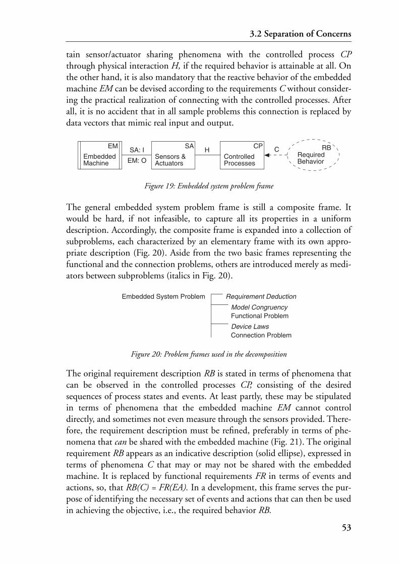
3.2 Separation of Concerns

tain sensor/actuator sharing phenomena with the controlled process CPthrough physical interaction H, if the required behavior is attainable at all. Onthe other hand, it is also mandatory that the reactive behavior of the embeddedmachine EM can be devised according to the requirements C without consider-ing the practical realization of connecting with the controlled processes. Afterall, it is no accident that in all sample problems this connection is replaced bydata vectors that mimic real input and output.

Figure 19: Embedded system problem frame

The general embedded system problem frame is still a composite frame. Itwould be hard, if not infeasible, to capture all its properties in a uniformdescription. Accordingly, the composite frame is expanded into a collection ofsubproblems, each characterized by an elementary frame with its own appro-priate description (Fig. 20). Aside from the two basic frames representing thefunctional and the connection problems, others are introduced merely as medi-ators between subproblems (italics in Fig. 20).

Figure 20: Problem frames used in the decomposition

The original requirement description RB is stated in terms of phenomena thatcan be observed in the controlled processes CP, consisting of the desiredsequences of process states and events. At least partly, these may be stipulatedin terms of phenomena that the embedded machine EM cannot controldirectly, and sometimes not even measure through the sensors provided. There-fore, the requirement description must be refined, preferably in terms of phe-nomena that can be shared with the embedded machine (Fig. 21). The originalrequirement RB appears as an indicative description (solid ellipse), expressed interms of phenomena C that may or may not be shared with the embeddedmachine. It is replaced by functional requirements FR in terms of events andactions, so, that RB(C) = FR(EA). In a development, this frame serves the pur-pose of identifying the necessary set of events and actions that can then be usedin achieving the objective, i.e., the required behavior RB.

EmbeddedMachine

RequiredBehavior

Sensors &Actuators

EM SA RBSA: I

EM: O

CControlledProcesses

CPH

Embedded System Problem Requirement Deduction

Functional Problem

Connection Problem

Model Congruency

Device Laws

53

3 Problem Decomposition

Figure 21: Requirement deduction problem frame

On this foundation, the three basic activities input, processing and output canbe further refined, which leads to two composite problem frames, each with anadditional auxiliary frame. This separation highlights the objective of the possi-ble dedicated models and tools for each of the two basic problem concerns:

• Functional problem frame: correct reaction to events in the environment.

• Connection problem frame: information transport between this environment and the control system.

3.2.1 Functional Problem Frame

The functional problem frame deals exclusively with the functionality of thecontrol system (Fig. 22). The machine to be built is the functional machineFM, whose purpose is to interact with the controlled processes CP in such away as to fulfill the required behavior RB in its guise FR. Since FM does notshare any phenomena directly with the controlled processes CP, the modelCPM of the controlled processes is introduced. This model substitutes thedirect connection by a notification scheme, whereby the occurrence of events Ewithin CP is signalled to FM as messages E’ (likewise A’ and A for actions in theother direction).

The solution for this problem frame is attempted by defining a behavioral rela-tionship of events E and actions A for the functional machine FM, according tothe required functional behavior FR (as deduced from RB and expressed interms of events and actions). The appropriate abstraction for this frame is toleave out any details not pertaining to the relation between the course of eventsin the environment and the inner states of a model.

Figure 22: Functional problem frame

RequirementDeduction

RD

C

EA

FR

RequiredBehavior

RB

FunctionalRequirement

EAFunctionalRequirement

ControlledProcessesModel

FM CPM FRCPM: E’

FM: A’FunctionalMachine

54

3.2 Separation of Concerns

An auxiliary frame is needed to establish the congruity between the controlledprocesses CP and the model CPM (Fig. 23). Essential phenomena events E andactions A, as called for by FR in the requirement deduction frame, are mappedonto respective messages E’ and A’. By clearly stating the difference between thereal events E, occurring in the domain of the controlled processes, and theirnotification E’ to the functional machine, problems caused by an inevitablyasynchronous connection are made explicit. Obviously, these must be dealtwith by the designers of the functional machine.

Figure 23: Model congruity problem frame

The functional problem frame is usually the most complex and at the sametime the one where alterations are to be expected until late in a development. Itis vital that models within this frame remain unaltered during structural adap-tation, such as operation mode transitions (see section 2.2.5).

3.2.2 Connection Problem Frame

In this problem frame (Fig. 24), the machine to be built is the connectionmachine CM, operating on domains FM and SA. Just as is the case for thefunctional problem frame, the connection requirement CR defines the abstractrelationship of domains in terms that in reality are not directly shared by adja-cent domains. As in the functional problem frame, events E and actions A arepostulated by the requirement. Events E (caused by the dynamics of CP) mustbe related to E’ (the corresponding message that makes this event known toFM), and action messages A’ (caused by FM) relate with A (that influence CP).The relation is again based on the model congruity frame from Fig. 23.

The requirement CR with regard to the interface to sensors and actuators SA isexpressed in terms of inputs I and outputs O. These are indeed phenomena theconnection machine CM shares with the sensors and actuators. But, inputs andoutputs neither appear in the original description of the required behavior RB,nor in the deduced functional requirements FR. This relation is established inthe auxiliary instrumentation problem frame (Fig. 25).

ModelCongruity

MC

E, A

E’, A’

ControlledProcesses

CP

ControlledProcessesModel

CPM

55

3 Problem Decomposition

Figure 24: Connection problem frame

The relation is determined by physical interaction H and gives rise to devicelaws DL. Since the device laws depend on unchangeable properties of the con-trolled domain (consisting of sub-domains CP and SA), they are given, whichmakes DL an indicative description. It specifies how events E and actions Arelate to inputs I and outputs O, respectively.

Figure 25: Instrumentation problem frame

Assuming a 1:1 relation of events E and actions A with their respective mes-sages E’ and A’ (established in the model congruity frame), the connectionproblem achieves just this transformation. Although the transformation is real-ized through inputs and outputs, this fact remains hidden from the functionalmachine, which is the main purpose of the explicitly proclaimed connection(Fig. 26). Therefore, the connection requirement CR is directly based on thedevice laws, in that CR = DL-1.

Figure 26: Connection transformations

FM

CM

FunctionalMachine

CN: E’ FM: A’ A

ConnectionRequirement

CRConnectionMachine

SA

SA: I CN: O

Sensors &Actuators

E

OI

Sensors &Actuators

ControlledProcesses

DeviceLaws

DL

SA

H

E, A

I, O

CP

E,A I,O E’,A’

MC

DL CR

56

3.2 Separation of Concerns

The connection problem frame’s functionality is basically implementation-ori-ented with a regular structure, so that a useful abstraction can be established onthe grounds of information transport in a generalized form. The connectionproblem frame unites input, the extraction of events contained in the new data,and the output.

3.2.3 Classification

The interfaces of domains are classified as being active, inert reactive, or both.Inert reactive domains initiate no events, but merely react to events initiated bya connected domain. The reaction affects some other shared phenomenon, butafterwards the domain returns to an inert state until a fresh shared eventoccurs. For the simple control problem from Fig. 18 the classification is con-genital: the control machine reacts to events emanating from the controlleddomain. As long as the controlled domain is inactive, no reaction, and henceno processing in the control machine, is needed.

This view is preserved in the functional machine, even including its solution,where it can be implemented as a reactive block. The same is true for the con-nection machine, as long as it is concerned with transforming action messagesoriginating in the functional machine to corresponding actuator outputs. Theycan be considered as the continuation of previous functional processing, i.e., inthis respect the connection machine is also inert reactive. However, there is adiscord with regard to events and event messages. While the conception ofevents (via inputs through sensors) from the controlled domain driving theconnection is convincing in the problem frame, realizations along these lineswould be difficult. They are possible, if the controlled domain and the sensorsshare all events. In this case, the hardware interface device could drive the con-nection actively (for example by raising an interrupt). Nonetheless, if continu-ous input values contain ‘events’, these events remain hidden from sensors andinput devices. Accordingly, interrupts cannot be generated at the interface andthe events must be obtained later by comparison against some threshold.

Figure 27: Domain classification

Functional Machine Connection Machine Sensors & Actuators Controlled Processes

controlled by Embedded Machine continuous

E’

A’

I

O

H

57

3 Problem Decomposition

Therefore, as far as the realization is concerned, the connection machine isdeclared the (only) active part in the system (Fig. 27). It induces inputs, detectsthe occurrence of events, and calls the reactive functional machine with theappropriate event message. It then relays action messages, the functionalmachine’s response, as output to the actuators.

Based on these precepts problem-oriented development methods with separatesolutions for the functionality and the connections to the physical processescan be built. Because the interfaces between the problem frames are explicitlymodeled and less prone to frequent changes than the frames themselves, devel-opment may progress independently. The separation remains intact even aftersystem deployment, a considerable benefit for later maintenance.

3.3 Abstraction‘Abstraction facilitates the understanding of complex realities, because itemphasizes an outline and omits details that are not relevant on a certain level.An abstraction of a set of objects is a description that applies equally well to anyof them. Each object is an instance of the abstraction, and there exists a one tomany relationship between the abstraction and the objects it describes’ (D. L.Parnas in [HPP81]).

Abstractions are models of reality. Useful models are accurate, simpler than real-ity, and understandable. To arrive at these goals, the purpose of the model mustbe well defined, and assumptions made during modeling clearly stated. Thevalidity of conclusions derived from a model is limited by the assumption cov-erage [Kop97]. Three spheres of activity can be discerned that correspond tolevels of abstraction (Fig. 28). Scopes for architectural and constructive modelswere given in the previous sections, whereas the final program code (an abstrac-tion from native machine instructions) is based on the definition of program-ming languages and the ways they are implemented on specific processors.

Figure 28: Spheres of activity

Components

Connection Functionality

Code

Architecture

Construction

Implementation

58

3.3 Abstraction

More subtle categories of abstraction are required within the spheres of activitythemselves, where developers work on many different levels of abstraction.Each level has its own set of description methods and tools, and it is very chal-lenging to maintain coherence throughout an entire project, practically stillaccomplished with just decisiveness and discipline. Often these problems areaggravated by wanting concepts that mistake omitting information for abstrac-tion (resulting in oversimplification). Valid abstract concepts according to theintroductory definition produce a number of views that engage one another ina formal way. If these relations are supported by some automatic mechanism,preserving project consistency is greatly facilitated. Dependencies are madeobvious, and the number of documents that needs maintenance is alsoreduced, since some of them can be produced automatically from others. Evenwhen this is not possible, the consistency of descriptions that depend on somehigher level of abstraction can be checked automatically.

The component architecture must contain all the information of both theoperational and implementation architectures. Their representation is infor-mal, or only partly formal, in contrast to the formal description of the compo-nent architecture. Therefore, conformance of these descriptions is subject tomanual examination. In the case of the operational architecture this is not aproblem, considering the description’s high level of abstraction and its orienta-tion towards elements in the environment. In the case of the implementation,the most detailed version of the possibly many different anticipated implemen-tation architectures must be covered.

The component architecture serves as a foundation in the elaboration of boththe functional model and the connection specification. System constructionmeans putting elements defined in the component architecture in concreteterms. The solutions must conform to the interface requirements postulated inthe architectural description. Not only is it possible to automatically check thisconformance, some element properties can also be directly imported. A sys-tem’s functional model is divided into clusters, then built using the given com-ponent arrangement, event and action messages, and possibly data and datatypes. In the connection specification the same definitions are used.

Specifications and models are associated with the implementation throughcode generators. Even if the development methods and teams are unrelated, themethods’ common foundation in the component architecture results in inte-gral implementations with the required functional and performance properties.The last step, from source to object code, is of course automated as well. It isconventionally performed by appropriate compilers and linkers.

59

3 Problem Decomposition

3.4 Practical Development SuitesThe three orthogonal aspects presented in this chapter can serve as a founda-tion of comprehensive tool suites. It is not sufficient to attempt developmentwithin the scopes laid out by problem frames, because they are not indepen-dent after all; the braces of an architectural description are needed to relate thedifferent concerns during development. It is not sufficient to describe a system’sarchitecture using components with arbitrary characteristics; components musthave specific implementation properties to get a perfect whole when the vari-ous pieces are combined (Fig. 28). It is not sufficient to relate behavioraldescriptions with any code that implements this behavior; the code must do soin a well defined way. To this are added the claims made in chapter 3, which alltogether might compromise the usefulness of such a tool suite for any practicalapplication.

The tool suite introduced in the following chapters lives up to the numerousconfinements. An unsuspecting observer might shrink from a developmentprocess crammed with even more obstacles than there are to begin with,whereas in fact the gross limitations of the design space turn out to be benefi-cial in finding lean and adapted problem solutions.

60

4 Architecture

Complex systems are built as a collection of a number of different more or lessindependent blocks. It is still common practice to define their interrelationonly implicitly in the interfaces of the active components. As a result, the sys-tem structure is hidden, and the generic character of components is compro-mised by embedded references to other components. A clearer picture ofsystem architecture as a framework for satisfying requirements requires con-cepts that treat not only components, but also the connectors1 between thesecomponents as distinct entities [Sha96]. Components are used to organize thecomputation and data into parts with a semantics and well-defined behaviors.The interaction among the components is represented by connectors. Theymediate the communication and coordination activities among components.The description of software architecture with appropriate languages and toolshas begun to emerge as a discipline apart from algorithms, data structures andother implementation details. Because its focus is on the configuration of com-ponents and connectors, it represents a top-down view of a system. It replacesthe now common informal ‘boxes-with-lines’ description, but also satisfiesdevelopers who need a detailed connection and interoperation model of thesystem that they have to build. Architectural views also provide the basis for asystem description in terms of the system’s constraints, which most often derivefrom the requirements. Numerous architecture description languages havebeen developed that not only cover syntactic aspects of components and con-nectors, but also permit to perform dependency and consistency analysis byincorporating behavior as formal annotations [AlG97, GaS94, Luc96]. Foranalysis, formal descriptions of the components and connectors are used to rea-son about system behavior. In the construction of a working system, functionalmodels (the foundation of any implementation) are associated with the com-

1. cf. architectural element connector vs. connection problem.

61

4 Architecture

ponents of the architecture. Systems developed in this way are based on anexplicit structural skeleton, which helps to maintain consistency among thevarious elaborated models. Finally, generic and well-defined architectural com-ponents are also a prerequisite for their reuse.

Architectural descriptions along these lines are commonly seen as a representa-tion of system resources and connections on a high level of abstraction, explic-itly in support of software development. Other areas of engineering use theterm architecture in a much broader sense, namely as the representation ofknowledge shared between a diverse team of experts from different fields.Adopting this view, an architectural description must embrace all system char-acteristics needed to make it the primary representation not only as a technicalbasis for software engineers, but also as a communication vehicle for projectmanagers, hardware engineers and domain experts. New points of view arethus introduced that must be matched in the description by adequate represen-tations of different aspects. The semantics of these representations permits anassociation of architectural elements with specific strands in the ensuing devel-opment process. But, considering the variety of its users, cognitive qualities arealso important, a claim that leads to representations closely matching meaning-ful properties of the application domain. The degree of complexity of a repre-sentation depends on the complexity of the controlled processes in theenvironment, but is made worse by variations introduced when the same par-ticulars are described differently by different people. This type of complexity iseffectively controlled by limiting the expressiveness of the description languageto what is needed [AnG99].

Of the three architectural descriptions introduced in section 3.1, two corre-spond to views from different fields, which are then integrated into a thirdview. Information from both the operational architecture, reflecting systemstructure as seen by domain experts, and the implementation architecture, whichembraces all conceivable hardware topologies, blends into the component archi-tecture. The foundation of the component architecture forms the pivot for allsubsequent constructive development work.

4.1 Operational ArchitectureThe ‘architectural’ views of domain (i.e., mechanical, electrical, chemical etc.)engineers are typically informal ‘boxes-with-lines’ descriptions. In spite of this,and because domain engineers think in terms of the application as a whole,their point of view is on a high level of abstraction. For a number of reasons,their way of partitioning a system must be replicated in the software structure:

62

4.1 Operational Architecture

• it is the basis for cost considerations and process management,• the cooperation across different professional fields is facilitated with a nota-

tion that is generally understood and accepted,• strategic decisions in a development are made in terms of components as

identified by domain experts.

Examples are the integration of legacy components, preferably including exist-ing control elements, or the need for independent development by differentparties. Having anticipated the separations along precisely defined interfacesdoes not only save time and expenses, it also helps preserve the integrity ofentire concepts.

The possible variety of ‘boxes-with-lines’ descriptions as an abstraction of com-ponents and their interconnection may seem immense (not to mention thesemantics inferred by the various designers). However, the object is abstractingfrom real machines and not from software and its mapping onto a hardwaretopology. Thus, the generic techniques that are applied in building machineryhelp confine the variety of architectural structures. For example, componentsin a drive train are arranged according to their physical connection, which islinear in general; components of a production line are related in harmony withthe flow of workpieces, etc. Both these examples suggest linear topologies alsofor their control systems, which may not be the preferred solution from thepoint of view of an installation’s control system. With additional components(which do not have a counterpart in the environment), hierarchy can be intro-duced into the structure, and the interfaces made simpler by lowering thenumber of interaction points. In the exemplary operational architecture for asmall robot (Fig. 29), the single additional component Head permits the real-ization of a star topology. Because the nature of interactions between the basiccomponents Motion, Handling, Navigation and Perception are not well definedat this stage, the otherwise necessary mesh interconnection is replaced by a sin-gle connection to each basic component. The advantages are that the interfacesremain stable even if more components are added, and that the details of inter-action among components can be resolved later, when Head is refined.

Figure 29: Robot: operational architecture

PerceptionMotion Handling

Head

Navigation

63

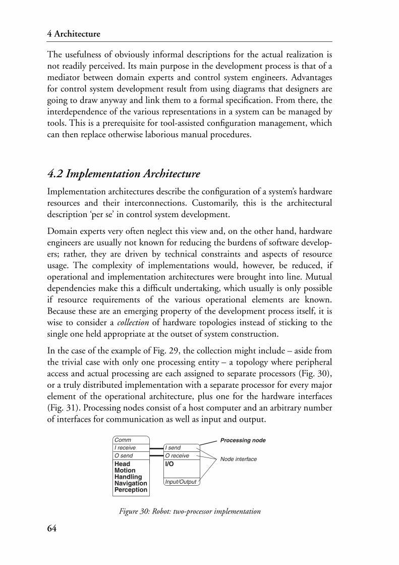
4 Architecture

The usefulness of obviously informal descriptions for the actual realization isnot readily perceived. Its main purpose in the development process is that of amediator between domain experts and control system engineers. Advantagesfor control system development result from using diagrams that designers aregoing to draw anyway and link them to a formal specification. From there, theinterdependence of the various representations in a system can be managed bytools. This is a prerequisite for tool-assisted configuration management, whichcan then replace otherwise laborious manual procedures.

4.2 Implementation ArchitectureImplementation architectures describe the configuration of a system’s hardwareresources and their interconnections. Customarily, this is the architecturaldescription ‘per se’ in control system development.

Domain experts very often neglect this view and, on the other hand, hardwareengineers are usually not known for reducing the burdens of software develop-ers; rather, they are driven by technical constraints and aspects of resourceusage. The complexity of implementations would, however, be reduced, ifoperational and implementation architectures were brought into line. Mutualdependencies make this a difficult undertaking, which usually is only possibleif resource requirements of the various operational elements are known.Because these are an emerging property of the development process itself, it iswise to consider a collection of hardware topologies instead of sticking to thesingle one held appropriate at the outset of system construction.

In the case of the example of Fig. 29, the collection might include – aside fromthe trivial case with only one processing entity – a topology where peripheralaccess and actual processing are each assigned to separate processors (Fig. 30),or a truly distributed implementation with a separate processor for every majorelement of the operational architecture, plus one for the hardware interfaces(Fig. 31). Processing nodes consist of a host computer and an arbitrary numberof interfaces for communication as well as input and output.

Figure 30: Robot: two-processor implementation

I/O

Processing node

Node interfaceHeadMotionHandlingNavigationPerception

O sendI receiveComm

O receiveI send

Input/Output

64

4.2 Implementation Architecture

In the topology of Fig. 31, some of the elements have their own peripheralinterfaces, additionally to the services provided by the node I/O. It is envi-sioned that Perception may need high input bandwidth exclusively (for bulkvision data), and Motion and Handling might require their own direct outputs.The granularity of a decomposition is up to the developers and their expecta-tions, but, since these are tentative architectures, overdoing it merely helps tokeep up future options. Thus, in the example, further refinement could lead tothe decomposition of single elements into clusters of processing nodes.

The degree of distribution in actual implementations can be less than proposedin any of the envisaged implementation architectures. In fact, most often thiswill be the case, as the implementation architecture merely sets limits to thedegree of distribution. This information is carried over to the componentarchitecture (see section 4.3), which defines deployable entities, and whosegranularity is based on the most detailed hardware topology provided.

Figure 31: Robot: fully distributed implementation

In the implementation architecture, resources take the form of generic unitsthat can be employed in a topology. Generic hardware units are processortypes, which may access peripheral devices and communicate with other nodesvia bus and network types. The quality of a proposed topology with respect tothe problem solution depends on attributes that can be measured quantita-tively. Resource adequacy is one such attribute, indicating that ideally, the pro-cessing demands of a component are just satisfied. Resource adequacy restrainsboth cost and system complexity, but it can only be asserted when the process-ing demands are exactly known, i.e., after concluding the constructive work ona component. This is also the main reason for postulating a separate architec-tural description (the component architecture) that is independent of anyimplementation architecture.

Another quality attribute is system reliability, which for systems with manyparts results from a combination of the mean time to failure (MTTF) of itscomponents. The use of redundant elements to achieve reliability and resourceadequacy is a difficult task in itself. For a systematic evaluation of these proper-ties tools exist that make use of genetic algorithms [NiB97].

RingComm

RingI send

Input/Output

RingI receive

RingI receive

RingI receive

Output

RingI receive

Output

PerceptionNavigationHandlingMotionHead I/O

Input

65

4 Architecture

4.3 Component ArchitectureOne goal in problem-oriented development of embedded systems is utmostabstraction from any envisaged implementation1. Furthermore, the actual con-struction of a system’s components is undertaken within a limited and preciselydefined scope, i.e., the global view is also abstracted away. This is the mainintention behind a formal component architecture that unites related compo-nents into groups, and defines the necessary interconnections between thesegroups. This top-down view of the system to be built is the pivot, which formsthe basis for the (compositional, i.e., bottom-up) construction work. The con-struction involves two separate problems according to the decomposition pre-sented in section 3.2. Because the component architecture is less prone tofrequent changes than the problem areas themselves, development mayprogress independently on the grounds of the previously defined architecturalelements.

The emphasis is on the kind of elements used in the architectural description.Instead of introducing ever new kinds of elements in the description of biggerand more complex architectures, scalability is achieved by replicating genericdesign elements with specific behavior and interface properties. One character-istic of this approach is the limited number of precisely defined element types(as advocated by [GaS94], where properties and relationships of existing archi-tectures are exploited), another consists in the separation of setting up thearchitectural description from actually allocating components onto processingelements. These two traits are in striking contrast with the notion of ‘architec-ture’ in the understanding of object-oriented methods, where the implementa-tion inherits the structure of what starts out as an architectural design (see forexample [LaH94]).

Architecture descriptions come in many guises. While they differ in theirdetails, there are some recurring elements, namely components, connectors,systems, properties, and styles [GKP00]. Components represent computationalelements and data stores of a system. The points of interaction between a com-ponent and its environment are called ports. Interactions among componentsare represented by connectors, which mediate communication and coordinateactivities among components. Their interfaces are defined by roles played bythe participants in the interaction represented by the connector. Systems areconfigurations of components and connectors. The configurations assign com-ponent ports to specific connector roles, thus restricting the component in the

1. Note that this is not contradicting section 4.2, which advocates a joint optimization of opera-tional and implementation architectures! Rather, the proposal to use a set of feasible hardware topologies at the beginning of a design process is in support of the abstraction called for here.

66

4.3 Component Architecture

interaction represented by the connector. In hierarchical systems, componentsand connectors may represent subsystems with internal architectures, a hierar-chy that is sometimes implicit. For example, a functional component’s internalstructure may be arbitrary, as long as it is within the constraints of the compo-nent’s ports and does not appear on the level of system architecture (seesection 4.3.2). Another example are connectors, which may expand to severalparts with their own active behavior (in case they link one processing entity toanother), or else disappear completely from an implementation (with a singleprocessor). Characteristics that cannot be expressed with structure alone areincorporated as properties of the elements of an architectural description, suchas the interaction protocol for an interface. Styles can be used to constrain ageneral purpose architecture description language by defining a specific vocab-ulary and ways of use for this vocabulary.

The constraints of the problem separation set guidelines for defining genericcomponents and component properties, including their roles in a later imple-mentation (which are derived from a component’s domain classification; seesection 3.2.3). Considering the declared separation of functional from connec-tive aspects, the component architecture specification does not need the expres-siveness of ‘universal’ architectural modeling languages. This separation alsopermits to hide the internal refinement (the local architecture, as it were) ofcomponents on the architectural level, and it emphasizes the differencebetween strong binding (within single components) and weak coupling(among components). Therefore, only a minimum of different componenttypes as well as ways of component interaction, hence connector types, isneeded (Fig. 32). The component architecture is a purposeful description thatbuilds on an implicit semantics of its elements1. It is based on a system-wideset of data, function, and interface abstractions provided by a restricted set ofgeneric architectural elements.

Figure 32: Component architecture notation

1. i.e., semantic properties of the generated implementations, brought about by the code generators.

Component

Connective component…with input and/or output

Unidirectional, bidirectional and multicastconnectors

67

4 Architecture

While verification and property assertions are not directly attempted, relevantproperties of the employed component and connector types can be expressedin general purpose architecture description languages with a sounder formalbasis (for example as a style in Wright [AlG97]) to make use of the elaborateanalysis tools available in these environments.

4.3.1 Specification

The emphasis in the presented approach is on its applicability to the develop-ment of real-world systems. For this reason, implementation details, such asconstant and data type definitions, have been introduced into the notation.Starting from the component architecture, construction of components isundertaken in different environments, according to their problem frame mem-bership. Since these environments produce their own code, type congruency isimportant to achieve syntactic agreement. On the other hand, there is theadvantage of generated implementations, consisting of modules with strictlycontrolled execution properties. Thus, each kind of component has inherentsemantic properties that can be relied on in the architecture specification. Theinitialization of components (and connectors, in case they are at all present inan implementation) can be included in the specification, whereas connectionclosure and halting of component computation need not be considered in non-terminating systems with a static architecture.

While the component architecture is explained with diagrams, actual architec-ture specifications are given in textual form. The specification language itself isdescribed in more detail in appendix A.

4.3.2 Components

The general notion of a component is that of an abstraction representing alocus of computation and state in a system. Components are elements that willbe refined as parts of either the functional or connection problems (see chapters5 and 6, respectively). The interfaces of components are called ports. Theydefine syntactic properties, namely the messages that are transmitted through aport and their types, valid types being all standard C types plus the previouslydefined custom types. Ports are qualified as being either sources or sinks.

Functional Component. Functional components can interact symmetrically viaasynchronous connectors, and they can be attached symmetrically or asymmet-rically to connective components (Fig. 33). Their constructive refinement is aCIP implementation unit (see section 5.4), which will result in a functional

68

4.3 Component Architecture

reactive block whose interface consists of a number of functions associated withmessages. A message is sent to this reactive block by calling the appropriatefunction (with possible data parameters); as a reaction the functional blockmay emit messages by calling one or several other functions itself. Port defini-tions of functional components include, in addition to messages, declarationsof these functions and their parameter types.

The semantic properties of functional components are derived from the behav-ior of their internal refinement. It depends, for example, on the transitionstructure of the process connected to a port, if this port can operate accordingto a specific communication protocol. A conceivable addition to the CIP gen-erators would be to extract traces from a completed functional model thatcould then be used for consistency analysis on the architectural level.

Figure 33: Functional component

Connective Component. Connective components accomplish the chores ofcommunication message handling, data input, event extraction, and data out-put. The event extractor component (Fig. 34) set aside, there are but three dif-ferent kinds of basic connective components (Fig. 35).

Figure 34: Event extractor component

As the name implies, event extractor components search the newly acquiredinput data for changes indicating events in the environment. Their specifica-tion associates binary patterns of discrete signals, or thresholds of quasi-contin-uous signals, with event messages. One of several lists of event priorities is

Functional COMPONENT

Dispatcher

CIP unit

CLUSTER n

CLUSTER 1…

I_MessagePort INStartNewPeriodInputReady(MessageList)

ErrorPort INErrorMessage

O_MessagePort OUT(MessageList)OutputReady

TransactionPort OUTRequestMessageMessageRejectedSetPriority

Port Specification

CIP unit

Dispatcher

Performance Table

Ports

Port Specification

Ports

EvEx COMPONENT

Extractor Specification

Extractor Specification

Event PrioritiesInput ValuesPatternsThresholdsMessages

TransactionPort INRequestMessageMessageRejectedSetPriority

DataPort INInputData

MessagePort OUT(MessageList)

69

4 Architecture

enabled, corresponding with the currently active mode of operation. Eventextractor components interact with input connective components (as a sink forinput data) and with functional components (as a message source).

Event extractor components are a special case among connective components,in that their specified functionality is tightly linked to the models of functionalcomponents. Not only their port message lists must coincide, but the relationof sensor phenomena with messages that is brought about must match theintentions the functional component is built on. For groups of event messagesthat are extracted from quasi-continuous input signals, traces are predeter-mined through the continuity of these signals and the inherent property of theextractor algorithm to preserve this ordering. However, nothing can be saidabout discrete input signals nor about correlations among different signals,since these depend (via input component) directly on the external processes.

Figure 35: Connective components

With the exception of the properties of communication components, whichdepend on the chosen communication paradigm, the port properties of theremaining connective components (Fig. 35) remain structurally stable, onlytheir types and sets of messages vary.

Ports

Input | Output | Communication COMPONENT

Connective Specificationone of Input, Output orCommunication Specification

Input Specification

DevicesSignalsFrequency ClassesConversionsFiltersInput Values

TriggerPort INTick

DataPort OUTStartPeriodInputData

ErrorPort OUTErrorMessage

Port Specification

Output Specification

Output ValuesConversionsSignalsDevices

ActionPort IN(MessageList)OutputReady

ErrorPort OUTErrorMessage

Port Specification

Comm Specification

DevicesProtocols

MessagePort IN(MessageList)

MessagePort OUT(MessageList)

ErrorPort OUTErrorMessage

Port Specification

70

4.3 Component Architecture

The functionality of connective components is limited to data conversion spec-ified in terms of peripheral devices and their data formats, signal conversionand verification methods, and abstract messages. There are no message tracesthat could be extracted before system deployment, because these traces dependon the behavior of the external processes.

4.3.3 Connectors

Connectors mediate the interaction among components, i.e., they restrict thebehavior of the attached components with protocols, sets of messages or per-missible traces. Rather than expressing these characteristics explicitly, the com-ponent architecture relies on implicit properties of the connectors used.Connectors guarantee syntactic and semantic compatibility between the com-ponents they relate, and need only be present as active elements in a finalimplementation if the components they connect are situated on different nodesin a multiprocessor installation.

There are two basic kinds of connectors, one (low-level) is associated with con-nective components and their interface to other connective components, thesecond (high-level) with functional components (Fig. 36). The first kind is typ-ically associated with bulk data transmission in a general form, requiringadapted low-level implementations tailored to the selected implementationvariant. The second kind provides asynchronous links across the unit bound-aries of functional components for potentially distributed implementations.

Figure 36: Connectors

Low-Level Connector. Some low-level messages are signals, while others con-tain data. Data transport can be simple or complex, depending on the differentways of implementation. As an example, consider a signal from a data input

I_EvEx EvEx_CIP

CIP_O

CIP_CIP

Low levelCIP COMPONENT 1 CIP COMPONENT 2

EvEx COMPONENT OUT COMPONENTIN COMPONENT

71

4 Architecture

component received by an event extractor component (connector I_EvEx inFig. 36). If both components are located on the same processing entity andshare memory, the receiver performs data reads directly from the shared mem-ory, whereas a distributed implementation contains a mechanism for copyingthe data before the signal message is delivered. In any case, with single writers,contention is not a problem.

High-Level Connector. There are two kinds of high-level connectors to con-sider. The first kind is a true high-level connector, in that it is applicable tocommunication messages, which are sent from one functional component tothe other (connector CIP_CIP in Fig. 36). These messages are queued and dis-posed of on processing. Queuing is required to maintain the time-ordering ofprotocols and processing sequences between communication partners. Thequeues are situated in the connector itself, permitting a choice of location forthe queue if sender and receiver are on different processing entities in a distrib-uted implementation.

The second kind is used to link connective components with functional com-ponents and vice versa. Event messages to a functional component are notqueued, instead they are pulled actively from their source, the event extractor(EvEx_CIP in Fig. 36). This evades problems associated with phase sensitivereal-time images that may become temporally inaccurate when functional pro-cessing cannot catch up with the queue contents. Like communication mes-sages, action messages that are sent by a functional component need to bequeued as well, to make up for transmission delays or asynchronous peripheralaccesses (CIP_O). In some situations, the occasional loss of a message may bepermissible, excluding messages that are discrete by nature (e.g., the setting of aswitch). An example where losses can be allowed are periodic output valuesoriginating from a control loop. Should the connector queue run out of space,as a last resort these messages can be weeded out.

To maintain the option of flexible component assignment to different process-ing entities, connectors are asynchronous by definition, even if a specificassignment leads to a synchronous implementation. The limitation to compo-nents with a run-to-completion semantics and a sole communication mecha-nism via asynchronous messages effectively limits the number of connectortypes. Connector implementations can rely on the execution properties of thegenerated component implementations, i.e., a number of fixed implementa-tions are available for each connector. To realize a connection in the resultingsoftware system, appropriate implementation mechanisms are chosen accord-ing to the physical location of the communicating partners.

72

4.3 Component Architecture

4.3.4 The Pivot

The component architecture combines the operational and implementationviews of architecture into a pivotal description that serves as a basis for con-structive development work. The pivot is strictly a basis only, in that it remainsuntouched by subsequent constructive work. Instead of refining componentsin place and within the context of an architectural description (as for examplein object-oriented methods [SGW94], or DisCo [KaM99]), actual system con-struction, up to generating complete implementations, takes place elsewhere.Given the paradigms of specification and modeling tools, and the properties ofassociated code generators used for solving the functional and connectionproblems, chances are that the emerging implementation parts will fit andresult in a working solution…

Another look at the robot example reveals that its component architecture(Fig. 37) takes into account the operational architecture from Fig. 29 on p. 63,in that it provides individual event extractor components for each subsystem(thus permitting separate development of these subsystems). It also takes intoaccount the most detailed implementation architecture of the ones provided(in this case the one from Fig. 31).

Figure 37: Robot: component architecture

Head

Perception

Motion output

Communication

Common input

EvEx_P

Video input

HandlingEvEx_H

MotionEvEx_M

NavigationEvEx_N

Handling output

73

4 Architecture

The selection of a specific implementation architecture can thus be postponedto when the processing requirements are more exactly known, i.e., towards theend of the constructive phase. Only then can the allocation of componentsonto processing elements be evaluated, according to processing and timingrequirements.

Dependencies in the development process itself are straightforward, concedingrelative freedom to developers working in separate problem areas, which arewell isolated by the pivotal component architecture (‘local change’ in Fig. 38).Alterations on the level of architecture or yet changes in system requirementsare reflected in the component architecture and necessitate adaptations in allproblem areas.

Figure 38: Development ripples

Global change Partial change Local change

Pivot

Implementation architecture

Operational architecture

Requirements

Connector specification

CIP Model

CIP Shell

t

74

5 Functionality

Mastering a specification language is not easy. At first sight, the translation offunctional requirements written in natural language into a formal notation ismore difficult than attempting implementation directly. This fact presents asubstantial negative incentive to the adoption of formal notations, although itforces developers to do without the advantages of abstraction on a high level,without the benefits of restrictions of a general purpose language to the subsetneeded in the solution of a specific problem, without code generation, andwithout the possibility of applying verification techniques.

Design and coding languages are rich expressive formalisms, permitting a vari-ety of solutions to given problems, although the full range of solutions is usu-ally much wider than is necessary or useful. Practitioners want to solvenaturally occurring domain problems, for which they do not need the fullexpressiveness of the languages they use. Guidance in the solution of com-monly occurring problems and restrictions in the use of language features arehelpful [MIS98], but even more advantageous are methods that provide ameans of formulating solutions in terms of the given problem.

To solve the functional problem means refining the relevant functional compo-nents of the component architecture (see section 4.3.2). Within the constraintsof the component’s port properties, the refinement can be structured in a prob-lem-oriented way. An appropriate method is the construction of a formal reac-tive behavioral model, often called an essential model [WaM85], because it isindependent of technical interface concerns. Its purpose is to specify the func-tional system behavior in subject-matter terms, based on the time-ordering ofevents. This is in accordance with chapter 3, where the connection of an imple-mented essential model to the real environment was established as a problem inits own right.

75

5 Functionality

5.1 State Machine ModelsFollowing the proposition made in section 2.1.1, the behavioral description isattempted with a notation based on finite state machines. Pure finite statemachines, introduced below, cannot directly be used for two reasons:

• systems described as one coherent model are too complex (because of the ‘state space explosion’ that afflicts any non-trivial models),

• the limited expressiveness of pure finite state machines rules out algorithmic descriptions (which are indispensable in practical applications).

While more elaborate modeling frameworks eliminate these shortcomings,these must be carefully scrutinized for their abilities to fit the component archi-tecture and to generate code that is efficient and executes deterministically.

5.1.1 Finite State Machines

State machines unite combinational circuits with storage elements. The con-tents of all storage elements make up the state a machine is in. The observablebehavior at its output depends on the input sequence and the machine’s inter-nal structure. A finite state machine is defined over sets of inputs, states, out-puts, and their interrelations. It can be modeled using a synchronous 7-tupleMealy machine , with

an input alphabet,a set of states,the set of permissible events while in state ,a transition function, , only defined for ,the initial state, ,a set of outputs,an output function, , only defined for .

Figure 39: State model of finite state machine

Figure 40: State diagram of finite state machine

X S Γ f s0 Y g, , , , , ,( )

X:S:Γ s( ): sf: f: S X S→× x Γ s( )∈s0: s0 S∈Y:g: g: S X Y→× x Γ s( )∈

s’ = f(s,x)y = g(s,x){…, x, …}

sx ∈ Γ(s)s’= f(s,x)y = g(s,x)

x/ys’

76

5.1 State Machine Models

Consider the simple example of a communication protocol with the followingspecification for the sender side:

• messages can be processed if they arrive while the sender is idle, otherwise they are lost,

• during processing, a copy of the message is stored, transmitted on request and a timer set,

• if an acknowledge is received, the stored message is deleted,

• when the timer expires, the message may be retransmitted on request.

This behavior is modeled by the example machine in Fig. 41, which exhibitsthe properties and

a message arrives,the message has been transmitted,the timer has expired,acknowledge received,sender is idle,message present,message is being transmitted,output, if the message was successfully transmitted.

Figure 41: Example state diagram: communication protocol

Practical applications of state machines face two major problems. One problemis their limited expressiveness, generally mastered with extensions that permitadditional functionality, the other regards the unwieldy size and blown-up statespace encountered in models of any non-trivial system. The size of statemachines grows exponentially with the number of states, a fact that precludestheir straightforward use in real systems. To overcome this impediment, practi-cable methods view systems as a collection of smaller state machines that bringabout the desired behavior of the system as a whole by mutual repercussion.They attempt to reconcile two contradictory claims: maintain an ongoing rela-tionship with the behavior of the external processes, and offer the benefits of awell-structured solution at the same time.

X a t x r, , ,{ }, S i m p, ,{ }, Y 0 1,{ }===

a: t: x: r: i: m: p: 1:

i

r/1

mt/0

pa/0

x/0a/0 a/0

77

5 Functionality

5.1.2 Hierarchy

A collection of state machines can be organized in various ways. Althoughmany reactive systems have a hierarchical structure describing the compositionof system parts, hierarchy is difficult to apply. The reason is that low-level inter-actions often have an essential influence on the high-level behavior of a reactivesystem. Composition hierarchies restrict interaction to local composition lev-els, but these are likely to clash with the actual problem structure. Anotherkind of composition hierarchy denotes nested state regions of an underlyingunfolded state machine (like in Statecharts [Har87]). The purpose of this hier-archical structure is clustering and refinement of behavioral descriptions,whereas interaction dependencies are not restricted by the state hierarchy. TheCIP method [FMN93], on the other hand, is a compositional approach, whichclearly distinguishes reactive behavior (of a process) from higher-order interac-tion (behavioral changes in subordinate processes). The master-slave hierarchyrelation of the CIP method is a set of associated state machines, whereas hierar-chical state machines in Statecharts represent compositions based on nestedstate sets.

5.1.3 Cooperation

In models that build on a collection of parts to describe complex behavior,cooperation of system parts within the same model is either synchronous orasynchronous. Synchronous cooperation, known from description techniqueslike Statecharts and ESTEREL [BeG92], is needed to model synchronouspropagation of internal interactions. Asynchronous cooperation, on the otherhand, which is supported by parallel modeling languages like SDL [Fae93],JSD [Cam89] or ROOM [SGW94], is necessary to express concurrency. Thetwo ways of cooperating also support the notions of loose coupling (asynchro-nous) and close binding (synchronous). Therefore, the CIP method makesavailable both synchronous and asynchronous methods of cooperation.

5.1.4 State Machine Extension

Data processing problem solutions are aptly described as transformational sys-tems, whereas solutions in process control show the characteristics of reactivesystems. For each, there exist matching and preferred descriptions, e.g., algo-rithms for transformational systems, and state machines for reactive systems.The descriptions are equivalent, but it is unwieldy to realize, say, a counter witha state machine (each value taken on by the counter must be represented by itsown state, resulting in blown up and unusable models). On the other hand,

78

5.1 State Machine Models

algorithmic descriptions of state-based behavior are hard to understand,because these descriptions are actually programs, and as such located on a lowerlevel of abstraction.

Inevitably, both these kinds of representation are needed to express the func-tionality of embedded systems; state-based models describe the functionalbehavior, whereas algorithmic descriptions are required for formulating com-putation, such as quasi-continuous control problems. Integrating algorithmicdescriptions into a process model is achieved more easily and preserves the highlevel of abstraction of this model, making it superior to the inverse. To this end,some means of incorporating algorithmic descriptions in a state-based solutionmust be provided. These extensions of the formal model allow the addition ofalgorithmic elements (i.e., program code) either to states (still a Mealymachine, with code executed upon entering the state via an arbitrary transi-tion), or to transitions (executed when the specific transition is triggered).

The equivalence of transformational with reactive descriptions is appropriatelyillustrated by the most simple of state machines with only one state and onetransition. The entire problem solution is contained in the single transition as acode extension, which executes whenever the transition is triggered. This setupeven has its uses when legacy code must be integrated into a project.

5.1.5 Semantics

The most widely used state-machine representation of behavior for reactive sys-tems is the Statecharts formalism and graphic notation [Har87, HaG96].While it presents intuitive ways to express hierarchy and concurrency, seriousdeficiencies concerning its syntax and semantics have led to the development ofmany variants. The variants basically fill semantic gaps with assumptions intheir implementations. Not surprisingly, merging these attempts into a coher-ent whole has proved impossible. Some of the more severe problems (describedmore fully in [vdB94], which also compares 20 Statecharts variants) include:

• the synchrony hypothesis, which postulates immediate reactions to changes of state in the environment (contradicts all practicable implementations),

• the notion of instantaneous states (that are entered and exited simulta-neously, i.e., in no time, according to the synchrony hypothesis), combined with events that are not consumed, but persist until the system has settled (may cause self-triggering and violates causality),

• no distinction between synchronous and asynchronous interaction, nor between external and internal events (global events and a global name-space impede the composition of separate models),

79

5 Functionality

• non-deterministic process activations and cyclic transmission paths allow infinite transition sequences (introducing non-deterministic behavior).

The CIP method, on the other hand, is based on a formal semantics [Fie00a].

5.2 Communicating Interacting Processes CIPUsing the CIP method [FMN93, Fie94, Fie99], the functional behavior of asystem is specified by an operational model of cooperating extended statemachines. ‘Operational’ means that the model is formally executable [Zav84].The CIP meta-model is based on a compositional mathematical formalismdeveloped for this purpose [Fie00a]. Mathematically, a system is defined as theproduct of all state machines comprised, corresponding to a single statemachine in a multi-dimensional state space.

CIP Tool1 [CIP00] is a framework of graphic and text editors supporting fullcoherence among various architectural and behavioral views. The tool is a com-ponent framework based on an object model implementing the CIP meta-model. Specifying models by composing and associating elements in a graphiceditor ideally fits the problem-oriented construction process of the method,providing more flexibility and intuition than language-based specification tech-niques. The tool generates code and exports model properties in various for-mats, suggesting verification and model checking by means of other tools.

Models are built with a notation of synchronous processes enclosed withinasynchronous clusters. Clusters are the coarse-grained elements combined inthe implementation unit of a functional CIP component as present in the com-ponent architecture. For a comprehensive view of the system to be built, all theunits defined in the component architecture can be dealt with simultaneously,and their interrelations defined on a functional level of abstraction. This isespecially important for implementations that may be placed into a multipro-cessor environment. The method permits to deal with both event-based andhybrid systems with integrated quasi-continuous processes. Event and commu-nication messages from the environment cause a transition in the receiving pro-cess, which activates other processes for his part. Transitions may generatepulses to other processes, as well as action and communication messages for theenvironment, and they can also contain additional code for data manipulationand control functions. Hierarchical system decomposition is further supportedwith a powerful master-slave concept.

1. CIP Tool®, partly developed at the Computer Engineering and Network Laboratory TIK of ETH, is now a registered trademark.

80

5.2 Communicating Interacting Processes CIP

Chain reactions initiated by a message cannot be interrupted; their executiondepends on the message itself and the internal states of all activated processes.A local architectural description (interaction net) together with explicitly speci-fied execution cascades set upper bounds to these chain reactions and preventsthe specification of cycles. Code generation for complete models is straightfor-ward and produces efficient and deterministic implementations.

A system is built with only a few essential elements (processes and channelsembodied within clusters), which are put together with appropriate glue parts(interaction net and pertaining pulse translation, message translation, inspec-tion and master-slave assignments). The basic elements are self-contained andkeep their interface properties even when detached from the surroundings.

In accordance with section 3.2.1, the construction of a CIP model is based ona virtual connection to the external processes. The virtual interface of the exter-nal processes consists of collections of event and action messages designatinginstantaneous subject-matter phenomena occurring in the environment.Events, often called discrete events, are caused by the autonomous dynamics ofexternal processes. Continuous behavior of external processes is captured bycomparing quasi-continuous input signals to defined thresholds, or by periodictemporal events with associated state values. Actions are environment phenom-ena caused by reactions of the embedded system.

Even if the task of associating environment phenomena with messages is not inthe scope of functional models (instead, it is resolved in the connection, seechapter 6), functional models are constructed with the concept of real eventsand actions. It is safe to do so on the grounds of the problem frame in Fig. 23,p. 55, which establishes congruity of real phenomena with their respective mes-sages.

In the final installation, the functional solution is contained within a reactiveblock (Fig. 42). The virtual connection becomes real through the implementa-tion of the connection solution, which transmits corresponding messageswhenever an event has occurred or an action must be produced.

Figure 42: Functional reactive block

Functional blockEvent Msg

Communication Msg

Action Msg

81

5 Functionality

5.3 CIP Constructive ElementsA CIP model is composed of a set of state machines termed processes, groupsof which are held together by clusters. Process cooperation is asynchronousacross cluster (and system) boundaries, synchronous or asynchronous withinindividual clusters. Formally, a cluster represents a state machine with a multi-dimensional state space, with the state of a cluster defined by the tuple of itsprocess states. Although clusters as well as processes represent parallel behav-ioral entities, their composition semantics is essentially different; clustersmodel concurrent functional blocks of a system, while processes representorthogonal and synchronously interacting components within a cluster. Hier-archical composition structures based on a simple ‘part of ’ hierarchy relationcan be introduced at both levels.

5.3.1 Process

Processes are modeled as extended finite state machines (Fig. 43). Process statesare represented by circles, transitions by labelled transition boxes. State transi-tions are activated by either an asynchronous message or a synchronous pulse.An input message, for which the current state has no outgoing transition causesa context error. Pulses, for which there is no transition, on the other hand, areignored. In a transition, one pulse and a message to each outport can be emit-ted.

Figure 43: Process structure

Data processing and algorithmic concerns are supported through state machineextensions, which consist of static process variables, data types for messages andpulses, operations and conditions. By means of state transition structures andoperations executed within transitions, functionality can be specified on twodifferent levels of abstraction. Variables, data types, operations and conditionsare formulated directly in C, the programming language of the generated code,and incorporated in-line. From the high level modeling point of view theseconstructs represent primitives, which add computational power to the purestate machine models. This pragmatic approach based on the implementation

T

S

S1 S2

S3

Pulse+Msg

Pulse

Msg

Inquiry

Inspection

82

5.3 CIP Constructive Elements

language permits the use of functions, data types and other elements fromexisting sources and libraries. It also presents a weak point, since C constructsmay inadvertently compromise the implementation properties of the func-tional model. Therefore, only a limited subset of the language is permissible,excluding for example all non-deterministic constructs, such as loops andmemory management functions.

The interface of a process consists of three parts (see also section 5.3.2):

• the communication interface is defined by one or more inports and out-ports. A port is specified by the set of messages to be received or sent. Each inport and outport is connected in the communication net to an incoming or outgoing channel, respectively,

• the interaction interface is defined by distinct sets of inpulses and outpulses,

• inquiries defined for a process permit the unobtrusive inspection of its inner states by other processes in the same cluster.

Process Arrays. Replicated processes are modeled as multidimensional processarrays. The multiplicities of the singular array dimensions are defined byabstract index types. Using common index types for different process arraysallows modeling of finite relations among process arrays, usually expressed bymeans of entity-relationship diagrams.

5.3.2 Synchronous and Asynchronous Cooperation

Communication. Processes of different clusters communicate asynchronouslywith each other and with the environment by means of messages, sent andreceived via channels. Channels model an active communication medium,which retains the sequential order of transmitted messages (Fig. 44 shows thecommunication channels and messages of a simple motor controller1).

Figure 44: Motor controller: channels and messages

Asynchronous communication implies that the write and the read action of amessage transmission takes place in different cluster transitions. Processes rep-

1. The motor controller system is further explained in subsequent examples.

CHANNELSCommands MESSAGES enable, disableSwitchEvents MESSAGES closeSwitch, openSwitchControllerEvents MESSAGES Standstill, Sample

ControllerActions MESSAGES MotOn, MotOff, MotValueIndicatorActions MESSAGES GreenOn, YellowOn, RedOn, LightOff

83

5 Functionality

resent receptive behavioral entities, which must accept messages delivered tothem at any time. The properties of those channels that are seen at the systeminterface must match the interface definition at the component architecturelevel. The transition structure of a process hooked up to a channel defines thetraces that this channel can accept or produce. This information can also beused for consistency checks.

The communication topology is specified by a graphic net model, in whichchannels are attached to process ports (Fig. 45). Source and sink channelsmodel the virtual connection to the environment, while internal channelsremain part of the model and do not show up at the interface.

Figure 45: Motor controller: communication net

Interaction. The processes of a cluster interact synchronously by means of multi-cast pulses. Pulses represent internally transmitted events. The straight directedconnectors of the interaction net (Fig. 46) define the pulse flow structure of acluster. Every connector has an associated partial function termed pulse transla-tion, which relates outpulses of the sender to inpulses of the receiver process(Fig. 47). Rhombic connectors declare state inspection (see below).

Figure 46: Motor controller: interaction net

Boss

ControllerEvents

SwitchEvents

IndicatorActions

ControllerActions

Switch

Indicator

Controller

Commands

Indicator

Switch

Controller

Boss

84

5.3 CIP Constructive Elements

A cluster is always activated by a channel message, which leads to a state transi-tion of the receiving process. By emitting a pulse, the receiving processes canactivate further processes of the cluster, which can in turn activate other pro-cesses by more pulses. This chain reaction is not interruptible and defines a sin-gle state transition of the entire cluster. Aside from generating pulses, activatedprocesses can also write messages to their output channels.

Figure 47: Motor controller: pulse translation

For models with multicast pulse transmissions, the structure of the interactionnet does not sufficiently restrict the potential pulse transmission chains, as non-deterministic process activations and cyclic transmission paths are possible ingeneral. To ensure deterministic pulse propagation, interaction is specified assequential multicast. The outgoing interaction connections of each process aretherefore defined as a totally ordered set. If a process emits a pulse, the receiversdetermined by the partial pulse translation function are triggered sequentiallyin the specified cast order to cause subsequent interaction chains. Thus, clustertransitions represent well defined sequences of process activations. To ensurebounded response times of system reactions, cyclic interaction paths must beexcluded, a model property that is enforced by the tool.

The specification of process reactions and pulse interaction by means of transi-tion relations and pulse translation functions formally defines a deterministiccluster behavioral model, from which all potential interaction sequences can bededuced. All potential interaction sequences can be shown graphically by thetool, either in the form of cascades (with processes as interacting elements), oras interaction trees, which also provide the details of pulse translation.

State Inspection. Conditions of a process’ state transition structure are allowedto depend on the states and variables of other processes of the same cluster.Read access to the data of a process is called state inspection; like in object ori-ented models it is granted via access functions termed inquiries. Unlike in pulsepropagation, which involves both the sender and receiver processes, aninspected process remains passive. Static context dependencies between pro-cesses by means of state inspection are declared as rhombic connectors in theinteraction net (Fig. 46), arrows denoting the direction of data flow.

PULSE TRANSLATIONSwitch start → Controller switchOnSwitch stop → Controller switchOffSwitch clearRequest → Indicator requestClearSwitch setRequest → Indicator requestSetController spinup → Indicator runningController spindown → Indicator stoppingController standstill → Indicator stopped, Switch stopped

85

5 Functionality

5.3.3 Behavioral Structuring

The state transition structure of a process specifies how the process must reactto inputs by state changes and generated outputs. Often, such a behaviorbecomes quite complex due to inputs that must influence the full future behav-ior of the process. An alarm message, for instance, must lead to behavior differ-ent from the normal case, until the alarm is reset. Dealing with these behavioralvariants in the same transition structure results in a superposition of the normaland the alarm case.

Modes. Since different ways of behavior that are conceptually distinct occurfrequently in practice, the full behavior of a process can be modeled by a num-ber of alternative behaviors, termed modes (Fig. 48). Each mode is specified byits own state transition diagram, based on the process’ static set of states, portsand pulses. A mode change does not affect the current state, which can onlychange when a transition in the active mode is triggered by an input. This rulereflects the fact that higher-order interactions do not alter the history of basicreactions. Behavior change without context change is typical of reactive sys-tems. Examples are the initialization, working, and shut down behavior ofdevice controllers, the modes of operation in classic control systems, or the var-ious error modes of protocol drivers in layered communication systems.

Figure 48: Master-slave hierarchy

T

S

T

S

Master process

Slave process

Modes

Pulse+Msg

M3

M2

M1

M1 M2

M3

Pulse Msg

Pulse+Msg

Pulse

Msg

86

5.3 CIP Constructive Elements

Master-Slave Relationship. Modes introduce higher-order interaction in theform of a master-slave relationship, in addition to and aside from the basicinteraction between processes and the environment or other processes. Higher-order interactions change the influence of basic interactions, while basic inter-actions cause state changes in the involved components. The generic master-slave pattern consists of a master, which can induce behavioral changes in aslave. “One man’s state is another man’s process” genuinely expresses the mas-ter-slave relationship.

Mode changes of a process can be induced by one or more processes designatedas master. This relation within a cluster is specified by a master-slave graph(Fig. 49). A triangle connects one, two or three masters to a slave. The graphmust be acyclic, a restriction complying with both the problem domain andthe quest for comprehensible system descriptions. When a slave is governed bymore than one master, a potential mode control conflict is resolved in a masteragreement associated with the master-slave connector. A master agreement,essentially a multi-dimensional table, defines how the mode of a slave is deter-mined in relation to the combined master states.

Figure 49: Motor controller: master-slave hierarchy

The active mode of a slave is determined by the current states of its masters.The association of master states and slave modes is specified by a correspondingmode setting table, which defines a total function from the Cartesian productof master states to the modes of the slave (the table in Fig. 49 relates masterstates and slave modes from Figs. 50 and 51, respectively).

Figure 50: Motor controller: Boss (as master)

Controller

Boss

MODE SETTING Controller

Boss STATE off onController MODE disabled enabled

off on

1disable

2enable

PROCESS BossMODE unique

87

5 Functionality

Thus, a mode change of a slave can occur whenever one of its masters changesits state. Even when the Controller process of Fig. 51 is in the off state in theenabled mode, its master can induce a switch to the disabled mode. The effect issimply that the motor will stay off when a switchOn pulse is later sent to theprocess. If, for functional reasons, a mode change should not occur in certainstates, it must be prevented by means of an explicitly modeled interactionbetween slave and master.

Figure 51: Motor controller: Controller slave modes1

A slave can itself initiate a mode change by sending a pulse to one of its mas-ters. This scheme is used typically when an error is recognized by a slave and itsmaster must then be triggered to induce a change to an error mode in otherslaves as well.

5.3.4 Extensions

To support data processing and algorithmic concerns, the pure state machinemodel is extended. Possible extensions are static process variables, data types formessages and pulses, operations and conditions. Variables, data types, opera-tions and conditions are formulated in C, the programming language of thegenerated code. From the high level modeling point of view, these constructs

1. The initial state of a process is marked by a token. High and low corner marks in a transition box indicate that the associated symbol denotes an input or an output message, respectively.

stopping

5 OSample

MotValue

4

standstill

Standstill

off

running

2

spindown

OSample

MotValue

PROCESS ControllerMODE disabled

off

running stopping

4

standstill

Standstill

2 OSample

MotValue

5 OSample

MotValue

1

spinup

OswitchOn

MotOn

3

spindown

OswitchOff

MotOff

PROCESS ControllerMODE enabled

88

5.3 CIP Constructive Elements

represent primitives, which add computational power to the pure models. Thespecified code constructs are included in-line in the generated code, a prag-matic way to easily incorporate functions and data types defined elsewhere.

Conditions. The same behavior as with a master-slave relationship can beachieved in the motor controller example with a completely different tech-nique, albeit at the cost of departing from the pure state machine model. Thetwo modes of the Controller process can be combined into a single mode,which brings about non-deterministic behavior. When the process is in the offor running states (gray in Fig. 52), there are two potential transitions for theinput messages switchOn and Sample, respectively. Associated conditions ren-der the process behavior deterministic. Such conditions can depend on theinput data and the values of the local process variables, but also, by stateinspection, on the states and variables of other processes of the same cluster.

Figure 52: Motor controller: Controller combined mode

Since the example attempts to replace the master-slave relation introduced inFig. 49, the switches of the motor controller depend solely on the Boss process.This process makes information about its state available through an inquiry(Fig. 53), added to the model of Fig. 50.

Figure 53: Motor controller: inquiry

stopping

1

spinup

OswitchOn

MotOn

4

standstill

Standstill

5 OSample

MotValue

running

2 OSample

MotValue

6 OSample

3

spindown

OswitchOff

MotOff

7switchOn

off

SWITCHESSTATE running MESSAGE Sample

TRANSITION 2 IF BossOnTRANSITION 6 ELSE_

STATE off INPULSE switchOnTRANSITION 1 IF BossOnTRANSITION 7 ELSE_

PROCESS ControllerMODE combined

INQUIRYint BossOn (void){return (STATUS.STATE == on);

}

89

5 Functionality

Operation. Another extension to the pure state machine model consists in add-ing code snippets to transitions (which are then marked with an O). An exam-ple are algorithms for continuous control, developed separately and used ascomplete building blocks. The motor controller contains two extensions of thistype, associated with transitions running:Sample:running, and stopping:Sam-ple:stopping, with the controller algorithms for running and stopping themotor, respectively. In the transitions triggered by switchOn and switchOff thesealgorithms are initialized (the description applies to both Figs. 51 and 52).

5.4 CIP Implementation UnitsImplementations of a CIP model are defined by partitioning the set of clustersinto implementation units. For each functional component of the componentarchitecture at most one unit is permissible, although several components canbe combined into a single unit. A unit is transformed into a reactive machinewith interface properties conforming to those defined in the component archi-tecture. The code of an implementation unit is made up of two parts, theCIP shell and the CIP machine, which are produced in two individual genera-tion steps.

Figure 54: Implementation of a CIP unit

CIP Shell. The CIP shell represents the interface of the implementation unit: itconsists of two linear structures of function pointers, one for the incoming andone for the outgoing channels. The CIP shell code is generated from the chan-nel specifications only, and so is independent of the modeled clusters.

CIP Machine. The CIP machine is a passive object implementing the reactivebehavior of the CIP unit; it is activated by channel function calls through theinput shell. Every call triggers a cluster transition from which channel func-tions may be called through the output shell.

CIP shell

CIPmachine

90

5.4 CIP Implementation Units

Once triggered by a channel message, the reactive machine runs to completion,i.e., it activates all processes involved in a cascade along the interaction tree,which is well-defined for each input message (see section 5.5.3). Performanceinformation about the worst-case execution path of each interaction tree,including transition operations, is obtained from an abstract model representa-tion that is generated by the tool along with the implementation code. Thepossible interaction paths of a model (the number of which is small comparedto models without interaction restrictions) are used for setting up an exhaustiveseries of measurement runs on the target itself. In the final implementation,performance data thus obtained are brought in for use by a simple run-timedispatcher (see section 7.2).

Furthermore, because of the cooperation of parallel entities defined within CIPmodels, there is no need to implement conceptual parallelism by means ofmulti-tasking. As a rule, only one CIP unit is present on a single processor. Theoverhead associated with task scheduling is thus reduced to the sequential dis-patching of just a few tasks, basically the ones already identified in Fig. 16,p. 49: input, processing, and output. The details of integrating functional reac-tive blocks into complete implementations are treated more deeply inchapter 7.

The environment-oriented development process of the CIP method allows thevarious CIP shells to be modeled at an early stage. The tool supports locking ofthese interface specifications for extended periods. In accordance with the con-straints set forth in the component architecture, the shells serve as semi-rigidjoints among the functional solution and its connection to the environment.Functional model development thus takes place in its own undisturbed scope,and it can proceed concurrently with ongoing activities in other domains.

Partitioning. System partitioning depends on the component architecture,which postulates separate deployment of its components onto their own pro-cessing entities. Clusters, representing very weakly coupled functional blocks,are the smallest entities assignable to an implementation unit. Therefore, afunctional element of the component architecture must be represented by atleast one distinctive cluster. For specific implementations, however, all clusterspresent in a system may be assigned to a single unit. In that case, communica-tion channels, i.e., the ones providing cluster interconnections, disappear fromthe unit’s interface, if desired. Their implementation, including buffers,becomes part of the generated functional code.

As an example, the internal communication channels of the robot controller(according to its component architecture in Fig. 37, p. 73) give rise to a com-munication net as shown in Fig. 55. Channel interface functions for the vari-

91

5 Functionality

ous connections of cluster Head with the working clusters and vice versa arepresent in the fully distributed implementation, whereas in a one-unit imple-mentation the entire network would disappear from the interface.

Figure 55: Robot: internal communication

The definition of several implementations containing dissimilar units and clus-ter partitioning is advantageous even in those cases where only a distributedtarget implementation is envisaged, as single-unit implementations can be eas-ily integrated into a simulation environment (see section 7.2.3).

5.5 Working with CIP ModelsWorking with behavioral models instead of programming requires a differentattitude towards the development process itself. Not unlike the plane taken tothe streets by a driver who mistakes it for a car, the new wings of a powerfulmodeling environment can make ‘programmers’ hit the walls. Some of the con-cepts that favor take-off are introduced below.

5.5.1 Functional Models within a Context

An operational behavioral model provides a well defined level of abstraction. Inaddition, the CIP method adopts the concept of environment-oriented behav-ioral modeling from the JSD method [Cam89]. This concept bases the devel-opment of control systems on a realized model of the environment inside thesystem to capture the essential behavior of the controlled processes. This leads

M_NavigationM_Handling M_PerceptionM_Motion

M_Strategy

Hd_HHd_M Hd_N Hd_P

H_HdM_Hd N_HdP_Hd

NavigationMotion Perception

Head

Handling

92

5.5 Working with CIP Models

to the construction of CIP models consisting of three parts, elaborated insequence (Fig. 56):

1. the virtual real world interface (events and actions),2. the behavioral context model,3. the functional model.

Figure 56: CIP high-level process interface

Events and Actions. The context of any functional model is not only deter-mined by phenomena of the environment, but also by the amount and qualityof the information that can be made available about this environment in theform of events and actions. Elaborating event and action collections representsa crucial development step, because it determines the level of abstraction usedto solve the functional problem. On the one hand, the collected events andactions must suffice to bring about the required behavior of the environment.On the other hand, the feasibility of the connection must be ensured by verify-ing that all events can be recognized, and all actions can be produced by meansof the available interface devices.

Events and actions can have attributes, which are transmitted as data with thecorresponding messages. An event attribute describes a circumstance of anoccurring event, such as the bar code read by a scanner. An action attributedescribes a circumstance to be brought about when the action is performed,like the position of a valve.

Events are classified into process events and temporal events. Process events arecaused by the autonomous dynamics of external processes, while temporalevents occur at prescribed points in time. In general, a process event is relatedto a discrete change in the external process. Discrete states in a model oftendenote a whole range of external process states, thus representing abstractions

CIP MachineEnvironment Connection

Controlledprocesses

Context

Complete model

Event & actionmessages

Events & actions Functionality

93

5 Functionality

essential for the required functional behavior. Examples are the level ranges of aliquid in a vessel, or the set of ready states of a complex device. Continuousstates are complemented by matching event extractor specifications that cap-ture the behavior of continuous processes (see section 6.4). Sampling events(such as the one represented by the Sample message in the motor controllerexample) are periodically occurring temporal events whose attributes are thesampled process states. Similarly, the embedded system influences continuousprocesses by repeated production of attributed actions.

While events and actions that are required and available are obtained by look-ing at the controlled processes, the process interface of functional architecturalcomponents is determined by the sets of related event and action messages.

Context Model. With the virtual real word interface given by the collections ofevents and actions, the first part of the model to be constructed is the contextmodel (Fig. 56). The purpose of the context model is to establish interface pro-cesses for the model and to connect them virtually to the environment. Theinterface processes are deduced from descriptions and process models of theenvironment. They receive event messages and produce action messagesthrough appropriately specified source and sink channels. The state transitionstructures of the interface processes describe the valid sequences of receivedevent and produced action messages, in other words, they represent protocolsof the virtual communication with the environment. Thus, the context modelformally describes the behavior of the individual external processes, as seenfrom the CIP model.

Functional Model. In the third step, the CIP model is completed by creatingfunction processes, which interact and communicate with the processes of theestablished context model. Modeling interface processes means understandingthe behavior of the external processes; but it also means anticipating the waythey will be controlled when the system is completed. It is by means of thefunction processes that the required behavior of the controlled processes in theenvironment is finally brought about. In a development, it is commonplace totackle the primary functionality of a system first, based on the normal behaviordefined by the context model processes.

Inevitable expansions must later be added to take care of behavioral variants,such as error modes, unexpected events, etc. Usually, the bulk of a completedsolution can be attributed to such expansions, which can only be added at thecost of breaking up the neat initial structure. With the CIP method, this struc-ture is preserved, because extensions are added to processes as what they genu-inely are, namely additional modes.

94

5.5 Working with CIP Models

5.5.2 Initialization

A system must be initialized in two phases, consisting of the initialization ofthe control system itself (low-level activities, such as bus and address modifierconfigurations, the initialization of peripheral devices, memory distribution,setting up the task structure; higher level activities such as initializing the innerstates of models and control algorithms), followed by an explicitly specified‘learning’ mode of operation. This mode with limited functionality endeavorsto copy the state of the external controlled processes to the inner state of amodel by observing the undisturbed or only gently influenced behavior of theexternal processes.

5.5.3 An Eye on Interaction

Interaction is a key issue in any system comprised of different parts, whetherthey are functions, classes, or model components on a higher level of abstrac-tion. It is difficult to keep track of interactions and interaction participants inany sizeable project, and the more recent programming paradigms have notmade it easier. In a modeling environment that does not restrict componentinteraction (like Statecharts, with its global event broadcast), the task is evenmore laborious. CIP Tool assists the developer not only by obliging her toexplicitly define interaction paths, but also through different graphic overviewsderived from the model itself.

Cascade. Cascades show sequences of potential process activation. This over-view abstracts from messages and pulses, but provides insights into a cluster’sstructure by displaying the longest possible activation paths, with individualprocesses of the interaction net as a root. As an example, the cascade of processController in Fig. 57 arouses suspicion, as Controller and Indicator appear twice.

Figure 57: Motor controller: cascades

Controller

Indicator Switch

Controller

Indicator

Switch

Controller Indicator

Indicator

Boss Indicator

95

5 Functionality

Interaction Tree. The more detailed interaction trees (Fig. 58, only shown forprocess Controller) reveal that this is not a design flaw, but indeed a possiblesequence. The sequence occurs, when the motor is reaching its stopped state,and the start button is being pressed at the same time.

Figure 58: Motor controller: interaction trees

Reporter functions export entire CIP models in selectable detail for documen-tation purposes. Other non-formal descriptions (such as UML-diagrams) mayalso be generated. They can be useful in highlighting certain aspects of a solu-tion, but present a one way path.

5.5.4 Behavioral Patterns

Many processes that are used to solve practical problems show the same recur-ring behavior, a simple example being that of a process with on-off behaviorthat can be used to model all kinds of switches and other discrete sensors. Formany of these common ways of behavior, abstract patterns emerge, similar tothose proposed in object-oriented design [GHJ95]. However, the two kinds ofpatterns are not on the same level of abstraction; while design patterns areabstractions of key aspects of program structures, CIP patterns present abstrac-tions of behavior.

Controller

EVENT_PORT

Indicator

Controller

EVENT_PORT

SwitchIndicator

Controller

Indicator

Indicator Indicator

Sample

spindown

stopping

stopped

standstill

stopped

start

stopped

switchOn

running

running

Controller

stopping

Controller

running

switchOff

spindown

switchOn

running

96

6 Connection

One characteristic of embedded real-time systems is their tight relationshipwith peripheral devices. The interfaces of these devices come in all flavors andmay lead to a plethora of different value encodings and timing properties in asingle system. Aside from complicating the initial development, the necessarychanges in systems that are inadequately structured can be severe if one of thesecomplex and restrictive external interfaces is replaced.

This problem was recognized early on and has led to the concept of ‘abstractinterfaces’, an attempt to isolate a system’s functional code from all interfacedevice details [HPP81]. An abstract interface may consist of virtual deviceswith device-like capabilities that are partly implemented in software. Virtualdevices simplify the rest of the software, liberating it from interface particularsand enforcing a disciplined and efficient use of resources. However, the idea ofreplacing real devices with virtual ones has its own problems. A virtual devicethat is based on a deficient abstraction may need to be changed at its interfacewhen the device is replaced (if the abstraction did not cover all possible devicevariants). On the other hand, internal changes may become necessary evenwhen the device remains the same (if device-independent functionality thatwas misplaced into the virtual device needs to be adapted).

Another problem is the implementation of virtual devices. Device accessrequirements frequently postulate their own protocols, which must be dealtwith locally and lead to independent entities with their own behavior and state.Consequently, very often virtual devices are implemented as tasks and inte-grated in a system’s scheduling scheme. Thus, a complex operating system iscalled for by the virtual devices even in those systems where the functional codealone could be implemented with a simple dispatcher [LaH94]. In these cases,the device interface tasks themselves introduce jitter and may undermine therequired sampling properties of individual signals (see section 2.1.2).

97

6 Connection

How can formal methods be applied in the connection domain? Complete for-mal descriptions would not only describe software, but involve the device hard-ware as well. This is infeasible for reasons of complexity, even if device internalsare known (usually they are not). Accordingly, developers depend on hardwareand software elements that have proved to be useful and reliable in other instal-lations [Web97]. If only parts of the connection are considered, however, for-mal descriptions are useful. Hardware items are then viewed as black boxes,and their low-level access routines left in the domain of programming,although the ways how these routines are combined are described formally.

The solution of the connection problem (see section 3.2.2) attempts to inter-face the functional code to a specific environment (Fig. 59). Because it must doso within the constraints of the component architecture (see section 4.3.3),updating input values or the opposite, setting new output values, are straight-forward duties for which a suitable abstraction can be found. The absence ofstructural difficulties encourages simple, sequential solutions for the three basictasks:

• data input, conversion and verification, with subsequent mapping to func-tional event messages,

• data output of converted and buffered functional action messages,

• communication with other nodes or across the system boundaries, received and sent via buffers as communication messages.

Figure 59: Interfacing the functional block

The chores of the connection fall into two categories: one is concerned withlow-level device access, data conversion and data transport (in distributedimplementations). The second category deals with event extraction. Therequired code and data structures are generated from abstract specifications

Functionalblock

Eve

nt

Msg

Actio

n M

sg

Comm Msg

Connection

Co

nn

ecti

on C

on

nectio

n

98

6.1 Device Access

that are given in terms of hardware devices, signals, and signal properties in thecase of input and output, and in terms of signals and event and action messagesin the case of event extraction (see appendix A). Code generators can exploitthe constraints of the component architecture persistently to achieve simplesequential solutions for each of the architectural components.

Aside from freeing developers of programming troubles, the main objectives ofthis approach are a uniform distribution of processor loads, code with proper-ties that fits the overall implementation scheme (see chapter 7), and the possi-bility to create implementation variants from the same specification. Simplervariants, such as the special case of simulation (where values are merely copiedfrom and to data vectors), are based on a subset of the specifications.

6.1 Device AccessAs noted above, working out the details of interfacing to the existent heteroge-neous peripheral hardware is a difficult task in itself. Input and output opera-tions on some devices are fairly complicated and must be made with multipleaccesses, possibly also requiring delay periods in between (Fig. 60). In addition,variations with regard to data width, channel number, multiplexer setup andpossibly filter and amplifier settings must be accounted for. In present-day sys-tems it is often not possible to exploit all the features of a hardware device,because it would be too tedious to program and impossible to master all poten-tial side-effects. Consider a 16-channel A/D-converter with the possibility toset parameters together with the number of the channel one wishes to convert.Filter and amplifier settings must be issued ahead of the conversion to allow forsignal stabilization, i.e., the current setting is influenced by the previous one,introducing dependencies between channels not otherwise related. In practice,this situation is often avoided by using the same settings for all 16 channels andenabling the round-robin conversion option many devices offer; a waste ofbandwidth for all but the signals with the highest requirements.

Figure 60: Device access sequence

t

setup read/write

Setup time

conversion

Conversion time r/w Access time

Controller

Peripheral device

Delay time

99

6 Connection

Selective specific multi-stage accesses combined with delays as shown in Fig. 60offer a potential for increasing performance, in that all the device accessestogether present a collection of tasks with precedence and exclusion relations. Aschedule for these tasks must satisfy the following requirements:

• a transaction consisting of the stages ‘setup–wait–read/write’ on an individ-ual peripheral device must be completed before another transaction may be initiated with the same device,

• delay times must be matched or surpassed.

Accesses as Tasks. The obvious solution of taking ‘task’ literally and castingdevice accesses to individual tasks that are schedulable by a operating system isinefficient. The cause of this inefficiency is the conversion delay, because therequired delay times usually are too short to justify rescheduling at the tasklevel. These delays thus remain periods where the processor idles until the nextread or write operation is allowed.

Accesses with Interrupts. Another solution uses the capability of many periph-eral devices to notify the processor of the end of a conversion themselvesthrough a hardware interrupt, freeing the processor in the meantime. Becausethe schedules of ‘normal’ processing are not independent of these interrupts(since scheduled tasks initiate device accesses in the first place), there is a ten-dency that interrupt service routines take their processing time from the sametasks on every occurrence, a fact that run-time schedulers cannot take intoaccount. Furthermore, interrupts introduce non-deterministic executionsequences, augmenting complexity in systems with many such devices.Although the overhead penalty is smaller than if rescheduling were attemptedat the task level, this approach leads to obscure run-time behavior.

Accesses in a Static Schedule. Fig. 61 illustrates the benefits of an alternativewhere the access routines of several devices are interleaved and the processoridle time minimized. The postulated delays are realized by inserting accesses toother devices, making use of the known device access times.

This technique is applicable to both input and output sequences, although in adifferent way. For reasons of efficiency, static solutions for the device accessschedules are preferable. While these are also feasible in the case of input access,output schedules are not statically determined, because they depend on thebehavior of the functional components. There, a simple ‘dynamic’ solutionconsists of two queues. One of these queues contains output accesses withouttiming constraints, which are used to realize the delays required for accesses inthe other queue. As in the case of input accesses, device access time must beknown in advance.

100

6.1 Device Access

Figure 61: Optimizing device accesses

From a timing point of view, input and output are separate activities, but thisseparation does not always hold for the devices themselves. Aside from usingsome of the resources in common (processor, memory, data bus, etc.), certainperipheral devices can deal with both inputs and outputs (e.g., interface mod-ules, motion counters/timers, etc.). If accesses are not serviced with atomicinstructions on these devices, exclusion relations may exist between ongoinginput sequences and outputs, and vice versa. Therefore, both input and outputaccesses must be defined in the same specification, which thus comprises allperipheral devices present in a system. The code generators are then able to addthe necessary mechanisms to prevent unwanted mutual interference.

6.1.1 Representation of Continuous Signals

The internal representation of input (and output) values usually deviates fromsensor and actuator data formats. The choice of internal representations isinfluenced by resource availability (processor performance, memory size, pres-ence of a floating-point unit, etc.), as well as by the physical process and thetechnology used in specific sensors and actuators (see section 2.1.3). It is diffi-cult to deal with measurement representations in different units (as exemplifiedby the many conversion-related incidents reported in [Risks]), so a commonformat is mandatory. Even if not required for accuracy reasons, the use offloat (e.g., 32 bit) in SI units is advantageous, and is a natural choice in sys-tems with a floating-point unit.

Recovered delay time

Sequential access

t

Dev

ice

t

Dev

ice

Interlaced access

setup readwait

101

6 Connection

Discrete signals are aptly represented by a single bit, but since these are notavailable in C (at least not in a universally portable way), bits are treated asmembers of data Bytes or words. ‘Conversion’ in this case involves breaking uptheir original hardware-oriented group membership to create new associationsbased on functional groups of discrete signals, the masks defined for thesegroups, and their timing requirements.

6.1.2 Encoding of Discrete Values

Input values from discrete sensors have a binary representation using one bit ina data word, the most compact way of representing information. Still, there aretwo reasons for rearranging this information. The first is that the original repre-sentation is dictated by the interface devices, which unite a number of such sig-nals (considering that these devices service 32 or more discrete signals at once).This results in a heterogeneous collection of signals where not all of its mem-bers share the same frequency class (see section 6.2).

The second reason is that it is unlikely that more than one bit has changedwhen a new set of values is read. Accordingly, there is potential for optimizingthe transmission scheme used to distribute such values. The given device repre-sentation dictates device accesses, because even when only some of the signalscontained in a device are needed in a given period, the device must be read atleast with the frequency of its ‘fastest’ members. However, in a distributed sys-tem with common input it is unnecessary to pass on all the freshly acquireddata to the working nodes.

Therefore, three variants of discrete value encoding and forwarding have beeninvestigated:

1. individual signals are masked in the sender and groups of values are formed according to the frequency class of each signal; further compression is nei-ther required nor possible, and the format is directly accessible in the receiver node (Fig. 62),

2. single data words containing discrete values are sent in compressed form; masking is performed upon expansion by the receiver,

3. entire data words containing redundant bits are sent uncompressed and are masked by the receiver.

Optimum use of the available channel capacity conjectures the re-encoding ofdiscrete signals in groups, corresponding with their specific frequency classes.On the other hand, the necessary compression and decompression in thesender and receiver, respectively, can be detrimental with regard to timingaspects. Actually, a comparison of the three different variants reveals only

102

6.2 Data Acquisition

minor timing advantages for sending compressed data, but it is superior inanother respect: if sampling requirements of signals not belonging to the high-est frequency class must be maintained (e.g., if they were postulated to achievelow-pass filtering, which rules out oversampling), the timing advantage is frit-tered away by the then necessary masking. In addition, forwarding outdatedinformation adds to the ugliness of the third solution.

Figure 62: Encoding of discrete values

Value output to discrete actuators is not affected by these considerations.Action messages are translated into predefined bit patterns, which are maskedonto a copy of the device output word. This copy is then written to the device.

6.2 Data AcquisitionNewly read raw input values must be converted to their internal representa-tion, verified for plausibility (if possible) and filtered (Fig. 63, left). In a decen-tralized system, incremental updates of operative input data are broadcastperiodically to all working nodes. Events pertaining to a specific node and itscurrently active event priority map are then extracted decentrally and used totrigger processing within the functional reactive block of this node.

• newly read values are available in their respective hardware formats (raw input data) and must be converted to the system’s predetermined standard formats (e.g., physical units),

Device Index

Bit Index

Class MED

Class HI

Class LOW

0 4 8 12

…

0 1 2 3 n1 2 1 14 1 5 6 8 9 10 13 0 1 5 6 12 13

…

0 1 2 3 n0 9 15 0 3 5 7 8 9 3 7 15 3 7 8 9 14 15

…

1 2 3 n0 2 6 7 8 12 2 4 12 14 2 4 10 11

…

Device 3

Device 2

Device 1

Device 0

Device n

0 4 8 24 28

Class MED

Class HI

Class LOW

not used

103

6 Connection

• the converted values are filtered and, if possible, pass a plausibility check. Data recognized as being faulty is marked invalid. In case a floating-point representation is chosen, invalidity is expressed by assigning the value NaN (Not a Number, IEEE standard indicating an invalid floating-point value),

• in distributed systems, the data must be forwarded to the working nodes for use by the event extractor components associated with functional units, and by functional units directly (Fig. 63, right).

Figure 63: Input data flow

Sampling frequencies of individual signals are postulated depending on proper-ties of the physical processes in the environment, as well as on the demands ofthe selected control algorithms (see section 2.1.2). A system’s base samplingrate is dictated by the signals with the highest timing requirements. This groupof signals leaves little margin for variations, and accordingly will simply be readwith the base sampling frequency, whereas all the other signals need only beread occasionally. Occasionally means that the point in time when a signal isread can be chosen freely, as long as the signal’s demands on sampling fre-quency and possibly jitter are met.

A seemingly simple solution would be to count intervals to define groups ofsignals that must be read in one sampling period (which is given by the signalswith the highest timing requirements). A group would consist of those signalsthat must always be read, plus the ones whose counter just expires. Unfortu-nately, this approach leads to extremely unbalanced resource utilization(Fig. 64). Even worse, unequal processor loads from one sampling period tothe other are not limited to data acquisition, instead they afflict all subsequentprocessing stages. Compared with the average utilization, hardware resources insuch a system become disproportionate, if only for the capability to cope withthe worst case (arrow in Fig. 64).

Functional block

Operative input datainput data

Input access

Conversion

Verification

Filter

Converted data

Verified data

Operative input data

Raw input data

input data

Event extraction

Functional block

Event messages

Operative input datainput data

104

6.2 Data Acquisition

Figure 64: Unbalanced capacity utilization caused by signal periodicity

Therefore, aside from minimizing absolute processor loads, the objective of aninput system must be to distribute work loads evenly among all periodic invo-cations, a demand impossible to fulfill manually. A feasible schedule for theinput task as a collection of smaller tasks with precedence and exclusion rela-tions is found statically and leads to a single sequential structure. The scheduleralgorithm solves the aforementioned problems: it eliminates possible idle timesand ensures practically equal processor loads for each invocation (Fig. 65).

Figure 65: Input access schedule for three frequency classes

Because any changes in the combination of devices or access frequenciesrequire recreating the schedule, this clearly is not a convenient method formanual implementations, although fortunately the affinity to general schedul-ing problems (as described on p. 100) make it suitable for code generation.

The specification for data acquisition is a high level description of signal prop-erties and requirements (see section A.2). Since this specification deals withperipheral devices, a description in terms of devices, signals, and signal conver-

Load

0 5 10 15 20 25 30 35 40 45 50 Period

0

1

2

3

4

5

6

Ace

sses

Worst case load

fLOW = n·fMED = 3·fHI

fHI

fLOW

fMED

1 2 3 1 2 3 1 2 3 1 2 3 1 2 3 11 2 3 4 5 6 7 8 1 2 3 4 5 6

1 2

t

ID

105

6 Connection

sions is appropriate. From this data, the generator creates an optimized andstatically determined schedule, using a signal’s timing requirements and thecorresponding device’s low-level functions for initialization, setup, access, con-version, verification and filtering. The execution and required delay times ofthe low-level access functions written in C must be profiled beforehand toenable the code generator’s static scheduling. Usually, the time required for anyread or write access depends on properties of the data bus, whereas delay timeis determined by the devices themselves. In practice, this signifies that theresults of just a few access measurements are applicable to a range of differentdevices, whereas delay times can be obtained from device data sheets. Theinput access schedule based on actual execution time measurements obtainedon the final target itself finds its complement in the performance analysis of thefunctional implementation (see section 7.1.1).

The advantages of the scheme come at the price of some specification andimplementation restrictions, which are in accordance with the chosen time-triggered implementation paradigm (see section 2.1.1):

• sampling jitter is kept out of input components only if there are no inter-rupts in the system (aside from a basic timer tick)1,

• all required sampling rates are mapped onto frequencies that are dividers of the base sampling frequency. Further simplification is achieved by assigning all signals to one of several frequency classes.

Assuming three signal frequency classes ( , , ), the generatedinput access schedule consists of a switch-statement with cases. Theschedule is generated heuristically (see section A.4.5), using the access time ofone signal to guarantee the necessary delay time for another signal, as inFig. 61. If no more access routines are available in a slot, or where they cannotbe used because of exclusion relations (when signals must be acquired by thesame input device), as a last resort plain delays are inserted into the schedule.

Unsatisfactory schedules and wasted processor time reflect deficiencies at thehardware architecture level, in that too few device accesses are available withwhich to create mutual delays. For small systems with few input signals theremay not be a satisfactory solution. In the example in Fig. 66 (with a frequencyclass relation of ), a small collection of input sig-nals with unfavorable exclusion relations causes the accumulation of delaytime. The plain delays result in a very low processor utilization of only 42%.

1. In implementations where interrupts must be used for dealing with certain devices (such as net-work and other communication interfaces), zero-jitter behavior of input components is still avail-able if interrupts are disabled during data acquisition.

fHI fMED fLOW

fHI fLOW⁄

fHI : fMED : fLOW 1 : 10 : 10

106

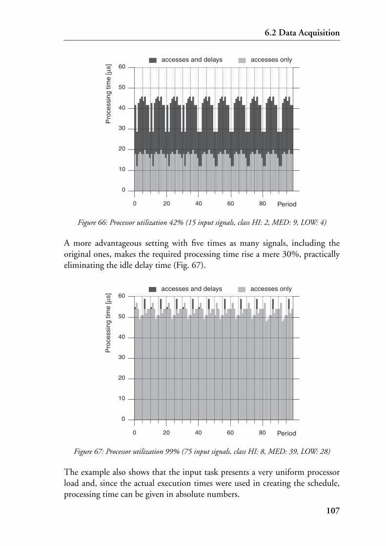
6.2 Data Acquisition

Figure 66: Processor utilization 42% (15 input signals, class HI: 2, MED: 9, LOW: 4)

A more advantageous setting with five times as many signals, including theoriginal ones, makes the required processing time rise a mere 30%, practicallyeliminating the idle delay time (Fig. 67).

Figure 67: Processor utilization 99% (75 input signals, class HI: 8, MED: 39, LOW: 28)

The example also shows that the input task presents a very uniform processorload and, since the actual execution times were used in creating the schedule,processing time can be given in absolute numbers.

60

50

40

30

20

10

0

Pro

cess

ing

time

[µs]

806040200 Period

accesses and delays accesses only

60

50

40

30

20

10

0

Pro

cess

ing

time

[µs]

806040200 Period

accesses and delays accesses only

107

6 Connection

6.3 Input Data DistributionThe task of distributing input data is very simple in single-processor imple-mentations, where it amounts to writing into global memory. In distributedsystems, however, communication bandwidth among processing entities oftenis a costly resource. Because input data acquisition presents an important andrecurring load of inter-processor connections, optimizing input data distribu-tion is worthwhile.

On the input node (or, in highly distributed systems, on an additional nodededicated to data conversion and distribution), continuous input values areconverted from a hardware format of, for example, 12 or 16 bit length to theirinternal representation, i.e., the format required by subsequent stages. If afloating-point representation is chosen, it cannot be optimized further by com-pression. On the other hand, channel bandwidth use in distributed implemen-tations is influenced by a suitable coding of entire data blocks, includingdiscrete values. The justification for choosing a specific method is based on thefollowing definitions and benchmarks:

: the inverse relation of a signal’s sampling frequency to the highest sam-pling frequency present in the system ( ), corresponding to the delayin periods in between successive accesses as generated by the staticscheduler,

: the number of continuous signals that must be read in the various fre-quency classes,

: number of continuous signals that must be transmitted in each period,

: data width of the converted input values in Bytes, for example for valuesof type float (32 bit, ).

Again assuming three signal frequency classes, plausible values (aside from ,which is always 1) would then for example be , .With a base sampling frequency , the resulting lower frequen-cies thus amount to and . These values wereused in the following comparison, where three different encoding variants areconsidered:

Variant ‘vector’. Package protocol: float, ..., float, float

The number of sent float values equals the number of continuous signals in afrequency class. Each signal value is allocated space in a vector; this vector issent in its entirety in each period.

Number of Bytes transmitted per period:

pfHI

m

m p⁄

ww 4=

pHI

pMED 10= pLOW 100=fHI 1000 Hz=

fMED 100 Hz= fLOW 10 Hz=

w m⋅

108

6.3 Input Data Distribution

Variant ‘indexed’. Package protocol: index, float, ..., index, float, stopbyte

Each read value is sent individually. In order to identify it, the signal’s inputvector index is also transmitted. A stop-Byte marks the end of transmission.The average number of values read in each period is , the index (1 Byte)being added to the actual signal value ( Bytes).

Number of Bytes transmitted per period:

Variant ‘masked’. Package protocol: mask, float, float, ..., float

Mask size is bits, rounded to the next Byte. Along with the newly read val-ues a mask is transmitted, where each bit corresponds to an entry in the inputdata vector. The number of set bits in the mask equals the number of valuesthat will follow in the current transmission, thus eliminating the need for indi-vidual indices and the stop-Byte.

Number of Bytes transmitted per period:

The effects of the presented variants on transmission efficiency when applied toone of the three frequency classes are summed up in Fig. 68 and Tab. 1. Asidefrom the emerged optimum solutions shown in italics in Tab. 1, in some casesothers could have been considered.

Figure 68: Input data distribution strategies

For reasons of simplicity and ease of implementation two of the variants werechosen and combined into a homogeneous solution: data in the highest fre-quency class is transmitted as a vector, data of the other classes in index-value

m p⁄w

w 1+( ) mp----⋅ 1+

m

m 7+8

------------- w+mp----⋅

0

5

10

15

20

25

30

35

40

45

50

Byt

es t

ran

smit

ted

per

cyc

le

0 10 20 30 40 50 60 70 80 90 100

Number of signals

vector (all classes)

vectorindexedmasked

Class LOW

Class MEDClass HI

109

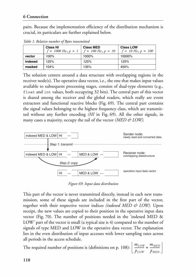
6 Connection

pairs. Because the implementation efficiency of the distribution mechanism iscrucial, its particulars are further explained below.

The solution centers around a data structure with overlapping regions in thereceiver node(s). The operative data vector, i.e., the one that makes input valuesavailable to subsequent processing stages, consists of dual-type elements (e.g.,float and int values, both occupying 32 bits). The central part of this vectoris shared among the receiver and the global readers, which really are eventextractors and functional reactive blocks (Fig. 69). The central part containsthe signal values belonging to the highest frequency class, which are transmit-ted without any further encoding (HI in Fig. 69). All the other signals, inmany cases a majority, occupy the tail of the vector (MED & LOW).

Figure 69: Input data distribution

This part of the vector is never transmitted directly, instead in each new trans-mission, some of these signals are included in the first part of the vector,together with their respective vector indices (indexed MED & LOW). Uponreceipt, the new values are copied to their position in the operative input datavector (Fig. 70). The number of positions needed in the ‘indexed MED &LOW’ part of the vector is small (a typical size is 4) compared to the number ofsignals of type MED and LOW in the operative data vector. The explanationlies in the even distribution of input accesses with lower sampling rates acrossall periods in the access schedule.

The required number of positions is (definitions on p. 108):

Table 1: Relative number of Bytes transmitted

Class HI,

Class MED,

Class LOW,

vector 100% 1000% 10000%

indexed 125% 125% 125%

masked 104% 135% 450%

f 1000 Hz= p 1= f 100 Hz= p 10= f 10 Hz= p 100=

Step 1: transmit

Step 2: copy

HIindexed MED & LOW MED & LOW

HIindexed MED & LOW

HI MED & LOW …

…

Sender node:newly read and converted data

Receiver node:overlapping datastructure

operative input data vector…

…

…

mLOW

pLOW-------------

mMED

pMED-------------+

110

6.4 Event Extraction

Figure 70: Input data copying

6.4 Event ExtractionThe functional reactive block is driven by event messages that are generatedwhen certain indications are discerned in the input data. In other words, eventsare extracted from the newest input data, which causes the generation of thepertaining event message (Fig. 63, p. 104, right). The tables that will be usedby the extractor algorithm are generated from specifications, which containconditions for each event (see section A.3). Event specifications may comprisetime events, discrete events related to binary signals and signal patterns, orevents associated with threshold values in quasi-continuous signals.

The connection of event messages with binary signals recorded as such fromdiscrete sensors is straightforward. When the signal changes, one of two possi-ble event messages is generated (separate messages are associated with the tran-sition from zero to one and vice versa). Since events are often associated withmore than one signal, predefined signal patterns (from the input specification)are used instead of just signals in the event extractor specification. The occur-rence of unspecified patterns has no direct effect, but since the change is inter-nally remembered, the previous event message is again generated when itspattern occurs. This behavior is useful if only one of the two events associatedwith a one-bit pattern is needed in the functional model, like the push of a but-ton.

For the other type of events (i.e., those buried within continuous signals), thesituation is less evident. Event messages associated with continuous signals aregenerated when the signal exceeds or falls below a specified limit. The limitscan be set arbitrarily within a signal’s range, however, their specification mustconform to certain conditions. Specifically, a hysteresis is required to permit

copied by receiver

-4 U -7 U -8 U • F I F F I F I F F F F I I I F FIdx Val End 0 1 2 3 4 -9 -8 -7 -6 -5 -4 -3 -2 -1

Sender data, i.e., transmitted data

Receiver data

Operative data vector on receiving node

…Class MED

Class HI

Class LOW

Data types:U universalI integerF float

…

111

6 Connection

proper switching of the extractor algorithm, which requires limit specificationsbe made with two values in ascending order (the extractor algorithm is given insection 7.1.2). If an event message of only one transition is needed by the func-tional model, nonetheless both limit values must be specified, the unused onemarked as VOID. The specification for the example in Fig. 71 is on p. 193).

Figure 71: Events in a continuous signal

The event extractor maintains the correct ordering of subsequent events, i.e., aslong as the information transport from the processes in the environment main-tains the continuity of events, no arbitrary message sequences will be produced.Furthermore, the event extractor is also capable of switching between a numberof different priority schemes at run-time. The currently active scheme is chosenfrom within the functional model, where all information regarding system sta-tus and desired system behavior is available.

A close correspondence of event extractor components with their associatedfunctional components results from the tight links of events and their eventmessages with the behavioral context model (see section 5.5.1). On the otherhand, the actual task of extracting events can be seen as an abstract activity,recurring in every conceivable system. Event extractor specifications thereforeneed only combine signals, their patterns and thresholds, with event messages.

6.5 OutputSystem output is generated when functional blocks issue action messages.These messages are converted, queued, and output before the current samplingperiod ends (Fig. 72). In distributed implementations, several functionalblocks may be located on individual nodes, so their action messages must firstbe transferred to and collected in output nodes.

101.0 99.0

1.0-1.0

°C

evaporate condensedew

112

6.5 Output

Figure 72: Output data flow

Contrary to the input, system output load cannot be distributed statically, asthe number of outputs depends on the specific transition structures encoun-tered in a cascade of the functional model (see section 5.5.3), as well as on theoccurrence of multi-stage hardware accesses. On the one hand, multi-stage out-put is needed for the same reasons as for inputs, namely because a peripheraldevice must first be set up before output data can be written. On the otherhand, a single action message may itself expand to a sequence of different out-put accesses. Consider the example of a positioning actuator. A new position ofthe actuator is selected by issuing a single action message with the position asan attribute, although the actual setting of the position consists of a number ofseparate steps: preparatory trajectory data include position and accelerationparameters, followed by commands to initiate the actual movement. While thebehavior could be described explicitly as part of the functional model, unclut-tering the functional model from this type of protocol is desirable.

Expanded output accesses are written to one of two queues. The first queuecontains accesses that may be written directly and as soon as possible. Accesseswith timing constraints, which in this case are delays that must be maintainedbetween write accesses on a device, are written to the second queue (Fig. 73).While both contain the previously measured access time, the queue for delayedaccesses also holds the delay relative to its predecessor element. Element inser-tion, which involves a linear search and moving of the elements in the rear, isusually not a problem since the queue is very short. Its length mainly dependson the number of items that cannot be dealt with in the same processing periodthat generated them, i.e., accesses with long delays. Because these should behandled explicitly in the function model, there is a limit on maximum delaytime in the specification.

Both queues are emptied by a simple output run-time scheduler. The delayedqueue has priority as long as its front element can be deployed directly, elsedelays are accomplished by inserting direct accesses (Fig. 73, right).

Functional block

Conversion

Converted data

Action Messages

Queue

Output access

Expanded data

113

6 Connection

Figure 73: Output access queues and schedule

Stubs for calling the conversion and/or expansion routines from the functionalmodel are generated using the same hardware-oriented specification as for theinput schedules, the profile data in this case also including information onaccess expansions if required (see section A.2). With this information, togetherwith the set of action messages from the functional model (see section 5.4)upper bounds on the processing demands of the output task can be found. Astatic table with the relevant values is computed for use by the run-time sched-uler.

6.6 CommunicationSince no conversions or any other modifications are required, the communica-tion interfaces amount to the simple queueing and forwarding of high-levelcommunication messages to and from the functional block (Fig. 74).

Figure 74: Communication data flow

A E G F HB C D JI

a b c d fe g

Delayed accesses Direct accesses

0 +4 +8 +9 +5+2

+11 +10

J 3 0 4 0I 3 0 3 0D 5 10 1 0C 3 11 1 1H 4 2 3 1B 4 5 1 2F 5 9 2 0G 3 8 3 2E 5 4 2 1A 3 0 1 3

j 3i 4h 3g 5f 5e 6d 3c 3b 4a 3

Acce

ss fu

nctio

n

Acce

ss ti

me

Acce

ss fu

nctio

n

Acce

ss ti

me

Rel

ative

del

ay

Sign

al g

roup

Sign

als

to fo

llow

t

Functional block

CommunicationMessagesQueue

Transmit

CommunicationMessagesQueue

Functional block

Receive

114

7 Implementation

The need to ensure coherence between high-level specifications and executablecode has been a long-standing obstacle to applying models and specifications inthe area of real-time embedded systems. The reason is that most of the time thestep from abstract descriptions to implementations is not taken automatically,at the least it involves manual intervention. Because in general, implementa-tions contain much more detail than is captured by specifications, practitionersare reluctant to abandon a program after careful adaptation only because somepart of it needs updating after changes in the specification. Instead of generat-ing a new version, they adapt the program manually to the changes, whichleads to programs gradually diverging from the high-level descriptions.

Therefore, the high-level source baseline ought to be the only description usedin the development of the parts of a system that can be described on a highlevel of abstraction. To be useful, it must be linked to the lower levels in thesame way as program source code is linked to object code, namely by auto-matic translation that is complete and does not require manual adaptation.This implies also that manually written parts remain untouched and that theexecution behavior of the implementation at the low level is maintained, whichis only possible if the generated code complies to definite properties that prede-termine its structure and execution behavior. These properties are independentof the particular functionality called for in the high-level descriptions.

On this prerequisite, variations in the generated code that are required for sim-ulation and for various target environments are composed automatically fromthe same configuration, with the component architecture assuring interfaceconsistency of any partial implementation with its complete counterpart. Thecode generators yield code that can be implemented as three distinct tasks withrun-to-completion behavior, either together on a single processor or separatelyon different processing entities. On a single processor, they operate in sequence

115

7 Implementation

in every period. The input task with its uniform execution time on each invo-cation presents a constant load, while the time demands for the processing task(which includes the event extractor and the reactive CIP machine), as well asfor the output task depend on the occurring events and hence the cascades thatmust be run through. Performance data obtained by measuring executiontimes of the functional code itself is used in the local extraction-processingcycle to make best use of the available processing time in each period (Fig. 75).

Figure 75: Execution sequence

An execution sequence proceeds as follows: the input task is triggered by aclock pulse with a period conforming to the highest sampling rate specified (seesection 6.2). At the start of each period the processing task’s local clock is reset.After the input task completes accesses and data conversions, control is handedover to processing. Processing deals with single event messages, each of which isrequested from the extractor algorithm. This is repeated until the remainingtime slot has become shorter than the worst-case execution time associatedwith the latest extracted message. Then, the extractor is notified and controlhanded over to the output task. The same happens when all events have beenprocessed before processing time expires. In both cases, the output task thenproceeds to convert and output the previously buffered output messages.

…

Input

InputData

ProcessingEvent extractor CIP machine

Sample Message

RequestMessage

Output

Action message(s)

Event message

RequestMessage Action message(s)

Event message

Event message

MessageRejected OutputReady

End OutputReady

(Period time limit endsevent processing)

(No more events pendingin current period)

StartPeriodClock

116

7.1 Code

7.1 CodeThe production of source code for real-time systems is practically alwaysundertaken with language subsets, non-regarding the actual choice of language.Even when not enforced by regulations of the application domain (cf. theguidelines for the automobile industry [MIS98]), the use of language subsets isa necessity in projects with multiple contributors. For languages such as C withits notoriously long list of flaws, the definition of a less precarious subset ismost important (see section 2.2.3). It becomes even more so if code written byhand and generated code must be combined into coherent applications withdeterministic properties. The major stumbling blocks are dynamic data struc-tures, recursion, and loops with possibly unbounded behavior. These featuresare not permitted, which preserves well-defined execution sequences, a precon-dition for automatic profiling.

Restrictions in the use of a language by barring all unnecessary constructs fromthe toolbox is also a valuable means to enhance program comprehension, anespecially rewarding measure in embedded systems with their characteristictime-periodic execution.

Memory. Memory is allocated statically, because dynamic memory manage-ment (for example using the malloc routine built into C) implies several risks.Allocations can fail, and being able to deal with allocation failures in a runningsystem increases complexity. Aside from possible memory leaks, allocating andfreeing leads to memory fragmentation, which is the cause for the allocationroutine’s non-deterministic behavior.

The static approach allows allocation, but not freeing, whereby allocation isperformed solely during initialization. If allocation is performed only once, asimpler routine without the overhead of block headers can be used instead of alanguage’s normal allocation routine. Another advantage is that this routine canbe disabled after completing the initialization.

7.1.1 Functional Code

The code that is generated from functional CIP models is efficient and deter-ministic. It is built as a collection of nested switch statements, which reflects itsgenuinely static properties, or in a table-based variant that introduces the sepa-ration of code from data. The code is truly reactive in that it remains passiveuntil one of its input functions is called. Upon such a call, a complete clustertransition is performed, after which the reactive block returns to its inert state.Aside from a number of housekeeping functions (e.g., those needed to advance

117

7 Implementation

the functional model’s own delay timers, or to perform read operations frominternal channels), the interface provides one specific function for each inputmessage specified in the model. Output functions must be defined in the envi-ronment and bound to respective function pointers during system initializa-tion. The functional block refuses to run if any of these are left dangling.

Processing time is present neither in the functional model nor in the connec-tion specifications. It is only by examination of the generated code that the per-formance on a specific target can be evaluated. Exhaustive performancemeasurements, which are extremely difficult to achieve with non-restrictedcode, get easy when the legion of possible paths through the code is limited.Because the performance profile includes all possible execution paths of thedeterministic code, the procedure gives the necessary assurance that an imple-mentation does perform according to the requirements.

If these measurements reveal processing bottlenecks, a way out can be soughtby distributing the work load onto different processors, or by softening therequirements on processing associated with certain events. In this case the mea-sured data together with the event priorities permit quantitative statementsregarding the performance degradation. It must be emphasized that exhaustiveperformance measurements on the final target are far superior to the vagueassurance that can be obtained from the combination of timing assertions in ahigh-level model and (inevitably) partial testing.

The generated code is compliant with the postulated restrictive implementa-tion demands, i.e., parallel structures present in the functional model are castinto a single sequence with deterministic behavior. Aside from generating themodules that implement the model’s functionality, a more abstract representa-tion of the entire model can also be produced. This representation can be usedfor creating other types of implementation, such as the table-based variantemployed in dynamic reconfiguration (see section 7.3). Performance analysis isalso based on the same representation. Each specified event message sits at theroot of possible paths through its pertaining cascade, for which a collection ofcode sequences (minus the action messages) is defined. This code is the execut-able counterpart of a unit’s interaction trees (Fig. 58, p. 96). The worst caseexecution path included in this collection must be found by measuring process-ing times on the target itself. Another excerpt of the abstract model lists onlythe sets of action messages belonging to each event with reference to the samepossible paths. These are used to determine upper bounds on the processingneeds of the output task. Aside from employing the data thus obtained to ver-ify that and how well an implementation will fit on a specific target, the samemeasurement results are also used by the processing task’s run-time scheduler.

118

7.1 Code

The functional code structure is explained using the motor controller exampleintroduced in section 5.3.2. Its implementation unit (containing a single clus-ter) accepts event messages and is capable of producing action messages asshown in Fig. 44, p. 83. The permissible traces in the input stream are deter-mined by the structure and interoperation of the receiving processes.

The transition structure of the example’s Controller process (Fig. 51, p. 88)shows the motor being either in state off, running, or stopping (the motor runsand stops under continuous control). Its transition triggers are the switchOn/Off pulses from the switch process, the Standstill and the periodic Sample eventmessages for the controllers from the environment. Its outputs consist of pulsesspinup, spindown, standstill, to the other processes and action messages MotOn,MotValue, MotOff, to the environment.

Two different controller algorithms are placed within the transitions triggeredby the Sample event and associated with states running and stopping, respec-tively. It follows from the diagram that only one of these controllers can beactive at any time, thus effectively limiting the required processing require-ments. The transitions leading to these two states contain the initializationparts of the controller algorithms.

The time demands for processing the event messages in the motor controllerexample show the processing limits of a specific implementation (Fig. 76). Theperiodic controllers triggered by the Sample event message present a recurringload in each period; they are scheduled first. If the worst case paths are taken,only one additional event message can be handled during a single period. Con-sidering the time scale and the improbability of these events arriving at thesame time (i.e., in the same sampling period), this may still be acceptable.

Figure 76: Motor controller: processor time demands

Sample

closeSwitch

Standstill

openSwitch

Input

Output

0t [µs]

Eve

nt p

roce

ssin

g

100

119

7 Implementation

7.1.2 Connection Code

Input. The static access schedule for system input is based on the relation ofthe chosen frequency classes (e.g., , , ) and implemented as aswitch-statement with cases (see section 6.2). Another switch-state-ment of the same size is generated for converting, filtering and verifying thenewly acquired raw data. The two switch-statements are independent func-tions, so they can either be deployed sequentially in a single task, or in differenttasks if required by specific implementations. The timing behavior is staticallydefined and known when the schedule is created, since the schedule itselfbuilds on the time demands of individual accesses (the performance of the low-level access routines must be measured beforehand and included in the accessspecification, see section 6.2).

Event extraction. The event extractor is an efficient implementation of a tableinterpreter. Since it deals with two kinds of events that are either associatedwith discrete or with continuous input signals, it consists of two parts (Fig. 77).Each part has two linear data structures, one containing the static information(i.e., event message function pointers and their associated patterns or thresholdvalues), the other holding information about the actual state (i.e., the last dis-crete data value seen at this input with the specified Signal_ID, or the region acontinuous signal is currently in). A group of entries in the continuous table isdelimited with the smallest and largest numbers representable in the chosenformat (-∞ and ∞ in Fig. 77, -FLT_MAX and FLT_MAX in the case of float).

Figure 77: Event extractor data structures

fHI fMED fLOW

fHI fLOW⁄

-∞

∞-∞

∞-∞

Sign

al_I

DM

ask

Actu

al v

alue

Even

t mes

sage

Patte

rn

Discrete Signals

Sign

al_I

D

Dow

n ev

ent m

essa

ge

Dow

n th

resh

old

valu

e

Continuous Signals

Up

even

t mes

sage

Up

thre

shol

d va

lue

120

7.2 Deployment

When the event extractor runs, the list of discrete events is searched sequen-tially until a change of signal value is detected. An event message is generated,if the new value matches one of the specified patterns. For events that dependon continuous signals, two comparisons are needed (one against each of thethreshold values limiting the region the signal has been in so far, see section6.4). Aside from the Sample event message that always has the highest priority,event priorities are based on their location in the active list (with the list orderdefined in the event specification).

Output. System output is asynchronous and performed in several stages. In afirst stage, action messages originating from the functional model are bufferedlocally to allow for possible asynchronicities of the output system. The majorityof output signals results in a single hardware access, but sometimes expansionto several accesses with time lags in between may be necessary. For this reason,in a second stage two different buffers are provided (see section 6.5). In the caseof a simple output signal, a plain FIFO buffer is used, while for multi-stageaccesses, an ordered queue with relative delays is necessary. As in the case ofinput access schedules, delays are realized through insertion of accesses to otherdevices, though in this case, a simple dynamic technique must be used. Theschedule is produced by reading from the two buffers in a round-robin fashion,either until they are empty, a new timer tick occurs or, in case of the secondbuffer, a first element is encountered with a delay time that has not yet elapsed.

7.2 DeploymentIn many embedded applications a collection of singular tasks has replacedmonolithic programs with the advantage of smaller scale and simpler struc-tures. Modularity and dynamic behavior at the task level should permit systemcompositions involving new parts as well as legacy code. The drawbacks ofthese techniques in hard real-time systems are countered with more efficienthardware in the case of speed considerations and testing in the case of unpre-dictability concerns. In the more cost-sensitive embedded systems segment theclaim for additional resources is not well received, because it is mandatory thatthese systems use the slowest possible processor and a minimum of memory.For these applications, progress made in hardware development must result inlower cost or reduced power consumption, rather than compensate implemen-tation deficiencies. Predictable response times, vital in safety-critical systems onthe other hand, are hard to achieve without static methods using componentswith deterministic properties.

121

7 Implementation

7.2.1 Scheduling

A task’s workload is characterized by its execution time. If the workload will beused for scheduling purposes, it is the worst-case execution time that must beconsidered. This, however, is a pessimistic estimation or measurement.Although the pre-deployment guarantee afforded by such approaches is highlydesirable, most of the time the required processing time will be inferior to theworst case, affecting scheduler efficiency and thus leading to poor processorutilization. This is especially true when the difference between the worst caseand normal execution time is great. Because it is difficult to measure worst-caseexecution times accurately, deadline violations must still be detected and han-dled in those systems where scheduling is based on these.

Dynamic Scheduling. Dynamic scheduling deals with tasks in an arbitrarysequence and unknown start times, where the various tasks operate indepen-dently and where interactions are not clearly defined [LiL73]. Solving theinteraction problem is postponed and these issues are handed down to a laterstage (i.e., run time). All types of dynamic scheduling are punished with con-siderable overheads aggravated by conceptual difficulties such as resourcedepletion and priority inversion; besides, their essential shortcomings withregard to satisfying timing constraints have also been shown [XuP93]. This isespecially true for preemptive techniques that create an infinite number of pos-sible schedules for a given problem and introduce additional conflicts withregard to resource usage.

Static Scheduling. Static scheduling, on the other hand uses detailed priorknowledge of the tasks’ processing requirements to find a feasible schedule[XuP93]. While this technique can guarantee the correctness of its solutions, itis overly pessimistic regarding asynchronous events, which tend to be sched-uled too often and therefore waste processing power. Even an inadvertent com-bination of both methods cannot do away with this disadvantage, as trulyasynchronous tasks still have to be scheduled many times only to verify that theassociated event has not yet occurred.

In both these approaches, input and output activities are implemented as tasksand scheduled in the same way as computation. Generally (except for exclusionand precedence relations), no assumptions about the nature of the tasks actu-ally running on a target are made. Since such knowledge is available and thetasks’ code confirms to strict limitations, a combination of static and dynamicscheduling techniques is possible that allows for high processor utilization, atthe same time guaranteeing low input jitter and predictable behavior (Fig. 78).The overhead of a complicated scheduler is avoided, because there are onlythree basic tasks. No preemption is used and the remaining dynamic decision

122

7.2 Deployment

within the processing task involves a mere table lookup that hardly introducesany overhead.

Figure 78: Global and local schedules

Run-time Executive. Even for a minimum implementation with three differenttasks, some kind of a real-time, multi-tasking operating executive is needed tokeep track of available system resources (CPU time, memory, etc.), and allocateor release them on demand. Its job of controlling and coordinating activities isgreatly facilitated when the tasks present in a system cooperate, implying that

• their execution time demands are bounded and deterministic, i.e., once scheduled, they can be allowed to run to completion,

• they can (and must) be deployed in a prescribed sequence.

On this condition, a simple executive is sufficient to run the well-coordinatedcode segments produced by the generators. Because all tasks in the system areallowed to run to completion, a dispatcher based on non-preemptive roundrobin multi-tasking is appropriate. With this type of scheduling, the executivecan be kept small and highly efficient, and it is perfectly possible to develop acustom piece of software. This approach avoids royalties in high-volume com-mercial applications and makes the executive’s source available for verification.Furthermore, in systems with limited program storage space such as 8-bitmicrocomputers, small code size and a simple call interface are essential.

7.2.2 Processing Scheduler

When the input task yields the processor, the event extractor generates theSample event message for those quasi-continuous processes running at thehighest frequency available in this system. From then on, the processing taskrepeatedly requests single event messages from the extractor. Each message trig-gers a complete cluster transition in the functional reactive block, and for everymessage there is a worst-case interaction tree that it may trigger. The scheduler

ProcessingInput Output

dynamicdynamic, with time limitstatic, fixed time

static, round robin, run to completion

t

123

7 Implementation

exploits the fact that worst-case behavior is the exception and message process-ing will usually not exhaust its allotted time slot. The processing task keepstrack of the current time and also records the time demands of all pending out-puts, i.e., the ones associated with ongoing event processing. Whenever a newevent has been extracted, the expected processing time in the table is comparedto the remaining time balance of the current period. If it conforms, the event isfed to the reactive block and the procedure repeated until an event occurswhose execution would not fit any more. If completion cannot be guaranteed,processing of a message must be deferred to the next period. It is important tonote that in this case the event message is withdrawn and not put in a queue,because this particular event may not be present in the input data the next timethe extractor runs (this characteristic, combined with sufficiently low samplefrequencies can also be used as a low-pass filter, e.g., for input key debouncing).Not having a queue for events at the same time effectively prevents processoroverloads and is also a prerequisite for switching between different event prior-ity lists.

In the period shown in Fig. 79 (using measurement data of Fig. 76), processingfor the event message Standstill would not fit into the remaining time budget inthe current period and is rejected. This type of scheduling is achieved withpractically no overhead, and it is worthwhile because worst-case executiontimes are hardly ever exhausted. Thus, in reality more events can be dealt withthan predicted by the static analysis. The slack time nevertheless remaining canbe exploited by non real-time tasks, which must be preemptable.

Figure 79: Processing task schedule

7.2.3 Implementation Variants

During development, different kinds of implementations are required to meetthe demands of simulation and partial target installations. If these can be con-structed from a single set of functional models and connection specifications,

Sample

closeSwitch

Standstill

Input OutputProcessing

Processing deadlinet

Task

s

slac

k tim

e

124

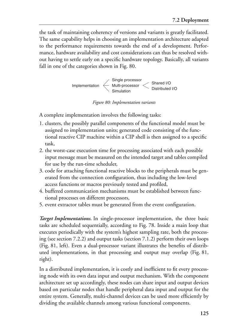
7.2 Deployment

the task of maintaining coherency of versions and variants is greatly facilitated.The same capability helps in choosing an implementation architecture adaptedto the performance requirements towards the end of a development. Perfor-mance, hardware availability and cost considerations can thus be resolved with-out having to settle early on a specific hardware topology. Basically, all variantsfall in one of the categories shown in Fig. 80.

Figure 80: Implementation variants

A complete implementation involves the following tasks:

1. clusters, the possibly parallel components of the functional model must be assigned to implementation units; generated code consisting of the func-tional reactive CIP machine within a CIP shell is then assigned to a specific task,

2. the worst-case execution time for processing associated with each possible input message must be measured on the intended target and tables compiled for use by the run-time scheduler,

3. code for attaching functional reactive blocks to the peripherals must be gen-erated from the connection configuration, thus including the low-level access functions or macros previously tested and profiled,

4. buffered communication mechanisms must be established between func-tional processes on different processors,

5. event extractor tables must be generated from the event configuration.

Target Implementations. In single-processor implementation, the three basictasks are scheduled sequentially, according to Fig. 78. Inside a main loop thatexecutes periodically with the system’s highest sampling rate, both the process-ing (see section 7.2.2) and output tasks (section 7.1.2) perform their own loops(Fig. 81, left). Even a dual-processor variant illustrates the benefits of distrib-uted implementations, in that processing and output may overlap (Fig. 81,right).

In a distributed implementation, it is costly and inefficient to fit every process-ing node with its own data input and output mechanism. With the componentarchitecture set up accordingly, these nodes can share input and output devicesbased on particular nodes that handle peripheral data input and output for theentire system. Generally, multi-channel devices can be used more efficiently bydividing the available channels among various functional components.

Single processorMulti-processorSimulation

ImplementationShared I/ODistributed I/O

125

7 Implementation

Figure 81: Single and dual processor implementations

Simulation. A special type of implementation is required for simulation, e.g.,using Matlab/Simulink [MAT99]. It is marked by the need to incorporate theentire control system into a single function, even if the target system will bedistributed. While the academic conjecture of using vectors to convey inputand output values holds nicely, there are a number of other problems that mustbe addressed. Namely, if stiff integration solvers are applied to the simulationmodel, simulation time must be expected to run backwards. Therefore, inputvalues need to be buffered before they are fed to the event extractor, or else thecontext models in the functional model could get out of step with the simu-lated reality, leading to context errors. Likewise, all output values must beupdated even when no changes occurred since the last call. This is handled byadditional functions that are only present in the simulation implementation(Fig. 82).

Figure 82: Simulation stages

Initialize

Wait(Clock Tick)Input

Extract

Process

Output

Convert

Dual processors

Initialize

Wait(Clock Tick)Input

Output

Convert

Initialize

Extract

Process

Single processor

discriminate()

extract()

remember()

handle_o()

u_prev[]u[]

y_next[]y[]

u[0]~ time

126

7.2 Deployment

The goal of a simulation is to validate as many parts of the final implementa-tion as possible. It is thus important to use exactly the same code that will bepresent in the later target system. For the same reason, input values, whichwould all be available in each new ‘sampling’ period in the simulation, must besampled using the same intervals chosen for the final installation. Therefore,the extractor algorithm and the tables it uses are also present in simulationimplementations.

Figure 83: Interface implementations for different modes of operation

Identifying Suitable Implementations. To identify suitable implementations,the following steps should be taken:

1. choose a set of envisaged implementation architectures (which must be con-tained in the component architecture); example variants are shown in Fig. 83,

2. for each variant:• generate complete implementations,• measure the timing performance of the worst case paths in the functional

block,

Fie

ld b

us I

Loca

l IC

omm

unic

atio

n

Loca

l IC

omm

unic

atio

n

Sim

ulat

or I

Fie

ld b

us O

Loca

l O

Loca

l O

Sim

ulat

or O

Target 1

Target 2

Simulation

Inpu

t 2In

put 1

Com

mun

icat

ion

Inpu

tC

omm

unic

atio

n

Inpu

t

Out

put 2

Out

put 1

Out

put

Out

put

Simulation

Target 2

Target 1

Connection generator Shell generator

Inpu

t CIn

put B

Com

m B

Out

put A

Implementation channels Operational channels

Inpu

t AC

omm

AO

utpu

t B

127

7 Implementation

• establish performance data of input, conversion, event extraction, and output (i.e., use data calculated by the generators for input and output, and perform timing measurements of conversion and event extraction),

3. compare measurement results with the timing demands set forth in the requirements and choose the optimum variant.

7.3 Dynamic ReconfigurationDynamic changes of configurations while systems are up and running havebecome commonplace in general purpose applications in a workstation envi-ronment. Today’s workstations can adapt themselves to the changing needs oftheir human users with minimal delay and yet maintain performance require-ments. In such reconfigurations new behavioral mechanisms become operativewithout affecting the currently active behavior. The flexibility achievable bydynamic reconfiguration ranges from creating and destroying tasks on a singleprocessor to reconfiguring entire task assignments in distributed systems.Despite the potential of dealing dynamically with functional entities that isoffered by many modern operating systems and programming languages, thesepossibilities are only reluctantly applied in the field of real-time embedded sys-tems. The reason is that dynamic methods entail the use of techniques that areadverse to the foremost goal in real-time systems, namely deterministic behav-ior. Still, these methods would be advantageous especially in systems that per-form under a number of distinct modes of operation. Examples of this can befound in flight control, where ground handling, take-off, cruise, and landingrepresent the different modes, or in communication systems that in one modeof operation service a large number of connections exclusively, or dedicate apart of their resources to administrative tasks under low load conditions in asecond mode. Since in purely static solutions the inactive parts unnecessarilyblock resources, dynamic reconfiguration may be indispensable for economicalor technical reasons.

7.3.1 Static Approach

Reconfiguration has two main areas of application. One is concerned with theon-line evolution of systems that must be available over long periods, while theother type of reconfiguration attempts to optimize resource utilization. Earlyattempts of the second type were mainly motivated by hardware limitations, aprominent example being the first control system for the Space Shuttle[SpG84]. In this system, code overlays were loaded from tape to fulfill the

128

7.3 Dynamic Reconfiguration

needs of specific modes of operation that correspond to the different phases ina single mission. Still today, optimal resource utilization is achieved through anumber of predefined configurations that form groups of functional compo-nents needed in specific modes of operation. Reconfigurable systems in thissense, with or without the inclusion of programmable hardware, consist ofoptimum algorithms within an adaptive component architecture. Systems withthese properties still run in situations where resources are tight, and/or theyperform better than the set of only partially active algorithms within a fixedarchitecture. The switching between various configurations, while preservingconsistency of the application data, presents an additional charge compared tothe routine obligations of real-time systems. Therefore, advantages can only beexpected from careful implementations.

Configurations are commonly defined explicitly, using dedicated languages.These languages deal with components and their instantiations, but abstractfrom component behavior. Because there is no connection between the levelwhere the various configurations are assembled and the lower applicationdomain, an additional step is required to identify dependencies and analyzeconsistent configurations off-line [FeL98]. This step may introduce inconsis-tencies caused by redundant information in the functional model and the con-figuration definition. Moreover, it is very difficult to manually find consistentconfigurations that satisfy the performance requirements of all tasks. Thisproblem can be evaded when a system’s functionality is described on anabstract level and configurations are based directly on this functional model –where they are implicitly present anyway.

Dynamic reconfiguration can be implemented either using features offered byan operating system or from within a programming language. If measures aretaken at the language level, they need to blend with memory management ingeneral and hence become dependent on implementation details of the lan-guage concerned. This may lead to memory fragmentation and non-determin-istic behavior, both major problems in systems that are required to run overextended periods. In practice this situation is avoided by the sole use of staticmemory assignment, or with preallocated memory pools of a fixed size. On theother hand, dynamic changes of system behavior that are achieved through anoperating system presuppose the use of dynamic scheduling techniques. Inthese techniques, a setup’s schedulability is based on static analysis. If theassumptions made for the analysis do not hold at run time, system behaviorbecomes non-predictable and timing constraints may be violated.

In the presented approach, implementation variants are built into the codegenerators, with the abstract models remaining completely untouched. One

129

7 Implementation

such variant is concerned with the mapping of functional modes of operationto the varying configurations of an implementation. The goal is efficient use ofthe primary resource memory while maintaining deterministic behavior andoptimum performance.

7.3.2 Reconfiguration Strategy

The reconfiguration strategy is built on the information about distinct modesof operation present in the functional model. This approach evades inconsis-tencies between the functional model and explicitly specified configurations,and it is also more efficient than low-level approaches that disregard the func-tional model entirely. Still, the two primary goals can be reached:

1. only code of currently active components is running, and2. temporarily unused data is eliminated to lower net memory requirements. If

a rise of resource demands in one component is complemented by a decrease in another, reconfiguration immediately benefits an entire system.

Static Code and Dynamic Data. Dynamic reconfiguration aims at extendingmechanisms that optimize processor utilization to also use memory as effec-tively as possible. Given the static environment and the necessity to avoid theuse of memory management at the language level, a promising option is to sep-arate code and data wherever possible. In the running system, the code willremain permanent, whereas data tables can be adapted to the current mode ofoperation. To this end, the nested switch statements of the functional code aregiven up in favor of tables and an interpreter engine. Separate tables are gener-ated that correspond with specific cascade subsets and hence with the demandsof the pertaining mode of operation. These tables can be handled dynamicallyat run time. As has been noted, the connection implementation must remainstable where it is concerned with the hardware environment. Thus, even inimplementations with different input schedules (which optimize processor uti-lization), only the event extractor tables are suitable for reconfiguration.

Compact Storage for Off-Line Tables. Fields of the state machine tables havethe types most adapted to their use by the state machine interpreter, i.e., intand pointer types. It is not necessary to store temporarily inactive tables in thisformat. Instead, tables not permanently required are stored in compressed formand loaded only upon entering the relevant mode of operation. The compres-sion is achieved by exploiting the fact that the name spaces of most table fields,i.e., processes, states, transitions and so forth are small and occupy only a fewbits. It would be possible to access data in the compressed tables directly duringexecution, but only at a great cost. Because the tables will be referenced fre-

130

7.3 Dynamic Reconfiguration

quently, it is worthwhile to expand them into a representation that is easilyaccessible by the target machine. The need for persistent state management fortemporary active cascades depends on a system’s mode switching policies. Ifmodes may be changed only when all processes in a cascade are in a definedstate, the state vector does not need to be remembered. Otherwise, processesmust be re-initialized with the values from the preceding state vector.

Run-Time Mechanism. In addition to a fully static implementation that mustdeal with event and communication messages alone, a change in the mode ofoperation is signalled to the scheduler just like a conventional (action) message.The purpose of this message is to trigger changes in the table as required forthis specific new mode. This chore is treated no differently from the executionof a cluster transition.

7.3.3 Example

In the robot example (its component architecture is shown in Fig. 37, p. 73), anumber of specific modes of operation dictate the work load that must be dealtwith by the various system components at different times (Tab. 2). For exam-ple, mode 1 calls for precise movement and high resolution perception only,mode 2 requires the robot to move along a trajectory with high speed, but lowprecision, performing only simple gripper operations, etc. In a naïve staticapproach the load variation in the components relating to different modes ofoperation results in a low average utilization of processing and memoryresources.

In cases like this, where disjoint modes of operation are well defined andknown in advance, a well adapted implementation can improve resource utili-zation considerably within the given static environment. In the following,improvements through dynamic reconfiguration for functional and eventextractor components are investigated.

The components Head, Motion, Handling, Navigation and Perception, togetherwith their corresponding event extractors all exhibit highly variable load char-acteristics that depend on the current mode of operation. The functional com-ponent Motion is examined in more detail for variations in its cascade

Table 2: Robot modes of operation

Mode Motion Handling Navigation Perception

1 Precision none Basic HighRes

2 Fast Coarse Best LowRes

3 Standstill Fine none HighRes

131

7 Implementation

dimensions and the influence of these variations on the rest of the system.Motion is placed in its own implementation unit as a single cluster; its interac-tion net is shown in Fig. 84.

Figure 84: Robot: interaction net (Motion)

Any temporarily active cascade subset is contained in the cluster’s interactionnet. A cascade subset’s extent directly influences the required processor andmemory capacities for a given mode of operation. Considering the multiplici-ties of the processes that deal with the four wheels, the requirement variationsare substantial (Fig. 85).

Figure 85: Robot: cascade subsets (Motion)

Cascade variations affect the event extractor tables insofar as processes withtheir own capability to receive messages may become inactive in certain modesof operation. In the cluster Motion this concerns the common and individualwheel speed control processes S_Com and S_Indiv (which are mutually exclu-sive). The table size varies from maximum in mode 1 (Precision for clusterMotion) to minimum in mode 3 (Standstill).

Requirement Variations. Resource requirements are summarized for the entiresystem and shown in Tab. 3 and Fig. 86 for memory (in Bytes) and processingtime (proportions over one period), respectively. The first row in Tab. 3 liststhe permanent requirement of each component, followed by specific additionalneeds per mode of operation. Implementations that make use of these overlaps

Motion_M Direction_Ctl

S_Com S_Indiv

D_RearWheel

Speed_Ctl

D_Front4

4

Standstill Fast Precison

132

7.3 Dynamic Reconfiguration

save 45% on memory requirements (using a maximum of 2250 Bytes at anyone time instead of 4090 Bytes), the minimum requirements being dictated bymode 1.

While no reconfiguration is needed to profit from the variable demands in pro-cessor capacity (Fig. 86), it is apparent that not all components could beaccommodated in one processing period if their maximum requirements fromdifferent modes of operation were to coincide. Because there is a possible trade-off of processing time granted to any component with the number of messagesthis component can deal with in a single period, the savings cannot be easilyascertained.

Figure 86: Modes of operation and processor utilization

Run-time performance. A sample situation that illustrates processor loads inthe vicinity of a change in the robot controller from mode 3 to mode 1 isshown in Fig. 87. Functional processing time has been summarized (light gray)to point out the role of the component Motion (dark gray). It can be seen thatthe transition from Motion being practically idle to requiring a substantialamount of processing does not affect the overall performance. Only the periodwhere the actual mode change takes place is dominated by the memory man-ager at the expense of other processing. At least, this routine is deterministicand the instances when it will be called are foreseeable and under control of thefunctional model and its modes of operation.

Table 3: Modes of operation and memory requirements

Mode Head Motion Handling Navigation Perception per mode

1…3 750 200 50 50 150 1200 (permanent)

1 100 900 0 50 0 1050

2 70 300 200 200 200 970

3 20 0 750 0 100 870

Processing

tMotion:Precision

Motion:Standstill

Motion:Fast

Hd M H N P

Hd M H N P

Hd H N P

Input

Input

Input

O

Output

Output

1

2

3

Mod

e

133

7 Implementation

Figure 87: Processor utilization at mode change

As shown in Fig. 88, the same mode change increases Motion’s dynamic mem-ory partition from zero to 900 Bytes, as required in the new mode. During theperiod in which the transaction takes place only the permanent requirementsare satisfied.

Figure 88: Memory allocation at mode change

0

10

20

30

40

50

60

70

80

Mode 3 Mode 1

other processingOutput

Memory manager

Motion

%

PeriodHeadInput

Motion: 200

Bytes

Period0

400

800

1200

1600

2000

Mode 3 Mode 1

Motion:Precision 900Standstill 0

dynamic

permanent

134

8 Hybrid III

8.1 Hybrid VehiclesThe history of hybrid vehicle drive systems reaches almost as far back as thehistory of motorized vehicles itself. Aside from the combustion engine, someearly car models were equipped with an additional electric motor to improvethe rather poor acceleration [Pie09]. However, this early form of hybrid drivesystems, along with the purely electric drive were soon superseded by strongercombustion engines that were not only reliable, but also economical thanks tomass production. Not until private vehicle traffic started to explode towardsthe end of the century and because of growing environmental concerns didthese concepts experience a renaissance. Purely electric vehicles still cannotequal the ease of use and the virtually unlimited operation range of conven-tional cars, mainly because of the unrivalled energy density of fossil fuels, sothat now hybrid cars have reappeared and even make it to full scale productionof important manufacturers [Hub97].

In Switzerland, traffic is responsible for roughly one third of the total energyconsumption. Aside from the railways that are operated electrically, this com-prises 98% of all fuels consumed. Furthermore, with an assumed averageenergy efficiency of 22%, internal combustion engines prove to be the consum-ers with the lowest energy efficiency altogether [BEW94]. As a consequence,higher energy consumption implies a greater pollution burden especially in thisfield. For mobile applications, the chief advantages and disadvantages of elec-trical versus propulsion systems based on internal combustion engines relate tothe energy conversion and storage, where they exhibit quite contrasting charac-teristics. In the case of the combustion engine, the high energy density of fossilfuels is the main benefit, its insufficient energy efficiency the major drawback(mainly caused by the inadequate use of the engine under part load). In com-parison, the chief advantages of electric drives consist in the wide range of

135

8 Hybrid III

speeds at a steadily high torque, combined with its high energy efficiency acrossthe entire operation range. The batteries needed as storage devices, on the otherhand, are poor performers, they are awkward to handle and present additionalproblems when they have to be disposed of. Hybrid concepts seek to combinethe positive properties of the two approaches and thus help reduce the energyconsumption and associated harmful effects of private vehicle traffic.

As the attribute suggests, hybrid vehicles have more than one way of storingand converting energy. The most well-known concepts involve combinationsof electric motors with internal combustion engines or gas turbines (Fig. 89).Apart from conventional batteries, additional (short-term) storage devices usedto absorb brake energy and to provide boost power under peak load may beinstalled, e.g., capacitors, hydraulic accumulators or flywheels. In principle twobasic concepts can be discerned. The two drive systems act simultaneously inparallel hybrids, while they are concatenated in serial hybrids [Bur92].

Figure 89: Hybrid concepts

8.1.1 Hybrid Concepts

In serial hybrids a combustion engine drives a generator to produce electricenergy that is either fed directly to the drive motor(s) or stored in capacitors orbatteries for later use. Because the vehicle is driven by the electric motor aloneat all times, this motor must be dimensioned according to the desired topspeed, cruise speed and acceleration. If an advantage is to result in comparisonwith conventional drive systems the energy efficiency of each component mustbe optimized and the control strategies for the energy flow chosen carefully.Serial hybrid designs are attractive because they can contain several electricmotors that are sometimes placed directly into the wheel hubs.

C

G

M

C

G/M B

Serial Hybrid Parallel Hybrid

C Combustion engineG Electric generatorM Electric motorB Battery

B

136

8.1 Hybrid Vehicles

Parallel hybrids have two essentially separate drive systems that can act upon thevehicle simultaneously. The electric drive in this case has only auxiliary func-tions and must mainly compensate weaknesses of the partially loaded combus-tion engine. In many of these concepts, the additional weight compensatesamply for the lowered fuel consumption, making reduced exhaust emissionstheir only advantage. The most simple of parallel hybrids can be attained withtwo drives acting on different vehicle axes, in which case they operate indepen-dently as two entirely distinct propulsion systems. On the other hand, if theyare coupled to a common shaft, the auxiliary motor can also take on the role ofelectric starter for the combustion engine. In such concepts, the possible disad-vantage of the electric motor having to rotate even when not in use may becountered by additional clutches with which to separate the two drives fromeach other.

8.1.2 Drive Systems and Energy Storage Devices

Putting together different drive systems and energy storage devices means tostrive for a compromise with the aim of combining the benefits each elementhas to offer. A short comparison of the key advantages and disadvantages sum-marizes the criteria that must be applied in the selection and evaluation of aspecific concept; these issues are discussed in greater detail in [Vez97].

If the energy density of the storage devices is compared, fossil energy is at a greatadvantage. The calorific value of regular gasoline amounts to approximately10 kWh/kg, which is in striking contrast with the 30 to 100 Wh/kg in batter-ies available today. The cruising range is directly dependent on it; for vehicleswith internal combustion engines it varies from 500 to 800 km, electric vehi-cles reach between 40 to 150 km. On top of that is the difference between sim-ple refueling and lengthy recharge times, an important point in daily use. Boththese disadvantages could disappear with the further advent of fuel cells, butsince these have not yet left the research centers, only conventional accumula-tor cells are examined.

When the energy efficiency is compared based on crude oil as the primaryenergy source, instead of just comparing the on-board converters (internalcombustion engine, electric machine), neither of the concepts shows any spe-cial advantages at rated load. At part load, however, the situation changes dras-tically, because electric motors exhibit a very high energy efficiency across theentire range of operation, whereas combustion engines suffer significant perfor-mance degradations when not fully loaded. Since a car’s energy demands onlyvery rarely reach rated load in normal traffic, this presents the major imperfec-

137

8 Hybrid III

tion of even state-of-the-art private vehicles. Conditions are similar with regardto engine torque. Combustion engines perform well only in a narrow operationrange, namely above a certain rotational speed. Electric drives, on the otherhand, can deliver maximum torque even at small rotational speeds.

The weight of a propulsion system and its mounting dimensions are lower forelectric solutions, but this is only true if the accompanying energy storagedevice is left aside. Emissions generated by road vehicles are for the most partnoise and exhaust gas from the combustion process. Electric vehicles producelittle noise and no exhaust gas (locally). Therefore they actually could help inameliorating the air quality of big agglomerations in the future.

Short-time energy storage devices permit the recovery of the vehicle’s kineticenergy while braking. Additionally, they can equalize peak energy demands andthus help improve the efficiency of the combustion engine. Unfortunately,most of the conceivable solutions exhibit only unsatisfactory overall energy effi-ciency, limiting the possibilities to mechanical storage devices. In general, theseare flywheels with a high energy density and direct mechanical coupling to thedrive system. Its installation is very complicated; it necessitates a continuouslyvariable transmission with an extended setting range and the associated elabo-rate control mechanisms [End96]. At the same time, a flywheel as short-termenergy storage device allows for intermittent use (duty cycle operation) of thecombustion engine, i.e., mechanical energy production and consumption actu-ally are completely separated. The vehicle is driven by the periodicallyrecharged flywheel, thus the combustion engine is operated in intervals only,but always in the range of its optimum efficiency.

A propulsion system for an economical clean air car can be built with a combi-nation of these elements, and without giving up the main advantages of con-ventional vehicles: unlimited cruising range and autonomy.

8.2 The Project Hybrid IIIHybrid III is the latest member of a family of hybrid cars developed at ETHsince 1990. As well as in the preceding projects, the intention was not to builda completely new kind of car, but rather to strive for optimum energy effi-ciency and for a substantial reduction of polluting emissions, using methodsfrom the boundaries of today’s technology. The main emphasis in this project ison the propulsion system, so that a commercially available vehicle was to be fit-ted with a new drive system. This novel drive system is a joint development ofseveral laboratories at ETH, and industrial partners [DHE93]. It features a gas-

138

8.2 The Project Hybrid III

oline engine, an electric motor, a flywheel storage device, batteries, and a con-tinuously variable transmission. Various clutches connect the gasoline engine,the flywheel and the transmission, while the electric motor sits directly on thedrive shaft. This assembly allows for all possible operation modes of a parallelhybrid, including duty cycle operation. Its most remarkable achievements aretwofold: an improvement of the combustion engine’s efficiency in extremeunderload operation, the prevalent situation in urban traffic, and best possibleuse of the available energy, because recovery is possible mechanically as well aselectrically. In urban traffic the vehicle is driven by the flywheel via the newlydevised continuously variable transmission. Because the normal setting rangeof 1:5 is traveled through twice, the much wider range of 1:20.5 becomes avail-able. With this expansion it is possible to translate high flywheel rotor speeds tosmall running speeds of the vehicle and vice versa.

Figure 90: Hybrid III drive system

The main features of the concept are:

• duty cycle operation: whereas engines in conventional cars run continuously and within undesirably broad rotational speed and power ranges, the com-bustion engine of Hybrid III is used intermittently and only in the vicinity of its optimum operating point,

• when braking, Hybrid III recovers this normally lost energy onto its flywheel with high energy efficiency,

• state-of-the-art exhaust gas cleaning combined with careful thermal balance management reduce harmful effects on the environment,

• shorter distances, namely within urban areas, can be covered electrically, hence completely exhaust-free.

C

G/M B

Hybrid III

C Combustion engineG/M Electric generator/motorB BatteryF FlywheelCVT Continuously variable transmission

CVT

F

139

8 Hybrid III

8.2.1 How it Works

Whenever the flywheel has slowed down and needs recharging, the gasolineengine is engaged. It works intermittently, i.e., it accelerates the flywheel withfull power to the desired rotational speed, after which it is immediately disen-gaged and turned off. Because the engine itself has been stripped of allunneeded inertia, starting and stopping can occur within a few revolutions.Operating ranges with unfavorable energy efficiency are therefore eliminated.On highways the system operates without the flywheel, because the load is suf-ficient to assure near-optimum consumption anyway. Exhaust-free driving inurban areas is possible up to approximately 60 km/h with the electric motoralone. In this operating mode the flywheel helps cope with peak demands thatwould exceed rated power output of the electric drive system.

8.2.2 Results

Measurement results confirmed the high expectations: all test bed measure-ment cycles showed reductions in energy use of up to 40%, in spite of the addi-tional weight of more than 300 kg. Energy consumption in the typical urbanmeasurement cycle ECE-15 amounts to 4.7 l/100 km for Hybrid III comparedto 8.9 l for the same car with a conventional drive system [Die96].

Figure 91: Hybrid III drive train

140

8.3 Hybrid III Components

8.3 Hybrid III ComponentsThe components of Hybrid III were designed and built by the individual aca-demic and industrial project partners in different places. Subsystems becameoperational with partial control systems that were identical to the one finallyinstalled in the vehicle itself. A detailed description of the mechanical designconcept is contained in [End96].

Internal Combustion Engine. The internal combustion engine is a standard1.3 l gasoline engine that has been adapted to the special needs of Hybrid III.Thanks to a modified control strategy the optimal specific fuel consumptionmatches full-load operation across the entire range, so that the intermittentcharging of the flywheel always happens with optimum efficiency and minimalconsumption [SGC96]. Other modifications affect the utmost reduction of themoment of inertia and the thermal comportment during duty cycle operation.The latter measures are necessary to protect the catalytic converter from unde-sirable temperature excursions.

Electric Motor. The electric drive consists of the electric machine [Kün95],power electronics and traction batteries, a battery charger, the vehicle powerfeed, and a braking resistance [Vez97]. There exist four main electrical operat-ing modes with vastly different requirements (starter, on-board generator, pro-pulsion, brake). Maximum permanent power is 6 kW for acceleration (limitedby the batteries) and 16 kW for braking. The higher value is only available inconjunction with the braking resistance, which is itself integrated into the vehi-cle cooling circuit.

Transmission and Flywheel. The transmission and the flywheel are the keymechanical components. The centre-piece in the i2-transmission is a continu-ously variable chain converter. Additional fixed gear ratios and a number ofhydraulically actuated clutches permit to travel twice through the converter(equivalent to having two such converters in series) and thus to attain the nec-essary high setting range of 1:20.5. The device features an energy efficiencymagnitudes above customary continuous vehicle transmissions, even whenoperating at feeble loads. The flywheel weighs 49 kg and its moment of inertiaamounts to 1.039 kgm2. It is designed for operation at a maximum rotor speedof 6000/min.

Thermal Balance and Exhaust Gas Cleaning. The combination of many dif-ferent elements with dynamically changing cooling and heating needs demandsa lot of the car’s thermal management, with the intermittent operation of thecombustion engine under heavy load presenting a special challenge. All drivingelements, together with the power electronics and the components for exhaust

141

8 Hybrid III

gas cleaning, are integrated into a heating/cooling circuit. Aside from the cata-lytic converter, a number of heat exchangers and latent heat registers areneeded. Heat flow is controlled by means of electrically operated pumps andvalves.

In contrast to conventional solutions, where temperatures and gas concentra-tions remain within restrained bounds, Hybrid III’s exhaust gas cleaning mustbe capable of dealing with the varying concentration ratios caused by the inter-mittent operation of the combustion engine. Whereas the temperature in thecustom-made catalytic converter is stabilized adequately with heat exchangersand a double-skin exhaust manifold, a catalytic material capable of toleratingthe greatly varying oxygen concentrations had to be sought at first.

Vehicle Interface. The Hybrid III propulsion system is built into a slightlymodified Volkswagen Sharan that has retained all its standard equipment. Thevehicle interface unites an especially designed multi-functional display and adrive selector lever with force feedback. All the other sensors and actuators donot differ from the ones found in conventional cars, effect of an early designdecision. Therefore, anyone accustomed to driving should have no problemswith this hybrid model. The most notable difference is an addition to the driveselector lever. Because the conventional hydraulically operated vehicle brakeswere left untouched, the lever doubles as input device to control braking viaenergy recovery. Position and force feedback is used to indicate the availabilityof the various energy converters and storage devices such as the flywheel, theelectric converter and machine, the accumulators, and the braking resistance.Contradicting user commands can likewise be resolved by manipulating thelever position. The other notable enhancement is the graphic display. In thedefault mode it serves as the car’s standard dashboard, but with its various otheroperation modes it can also double as a measurement value readout. An arbi-trary number of graphic screens can be defined with arrangements of signal andinner state displays. Engineers driving the car can choose dynamically fromamong these pages to focus on individual areas of interest.

Control System. The five principal components that make up the propulsionsystem for the Hybrid III car obviously must be united for the final installationin the vehicle, where they act together under the coordination of the sameregime. The same is true for simulation implementations, for which all compo-nents must be contained in a single functional block that integrates into thesimulation environment. Nevertheless, these components form coherent enti-ties all by themselves and as such they were to be developed and tested. Sub-systems became operational with control systems that were identical to the onefinally installed in the vehicle itself. Partial systems unite elements that have

142

8.3 Hybrid III Components

their own, independent processor capacities in the control system. Therefore, asolution had to be sought that could integrate these different operation modeswithout imposing too many changes when converting from one to the other.

Figure 92: Hybrid III system structure

Gears &Clutches

CombustionEngine

ElectricMotor

HeatTreatment

SystemInterface

Control System

143

8 Hybrid III

144

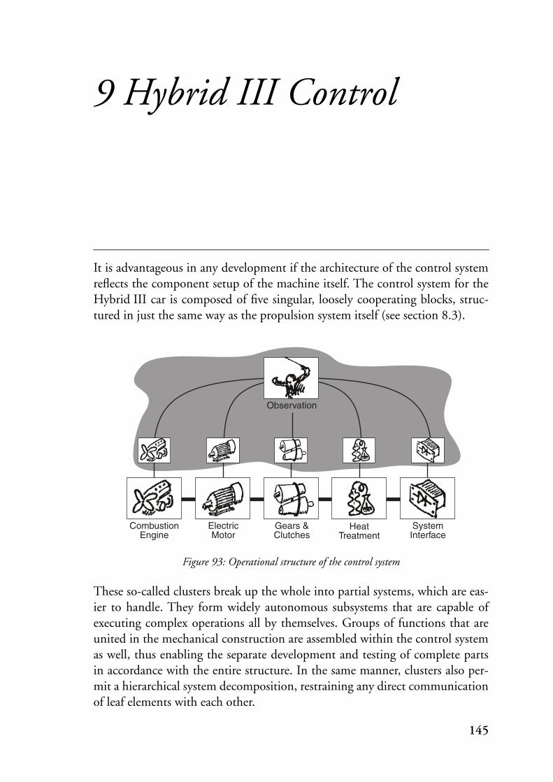
9 Hybrid III Control

It is advantageous in any development if the architecture of the control systemreflects the component setup of the machine itself. The control system for theHybrid III car is composed of five singular, loosely cooperating blocks, struc-tured in just the same way as the propulsion system itself (see section 8.3).

Figure 93: Operational structure of the control system

These so-called clusters break up the whole into partial systems, which are eas-ier to handle. They form widely autonomous subsystems that are capable ofexecuting complex operations all by themselves. Groups of functions that areunited in the mechanical construction are assembled within the control systemas well, thus enabling the separate development and testing of complete partsin accordance with the entire structure. In the same manner, clusters also per-mit a hierarchical system decomposition, restraining any direct communicationof leaf elements with each other.

Gears &Clutches

CombustionEngine

ElectricMotor

HeatTreatment

SystemInterface

Observation

145

9 Hybrid III Control

An additional cluster with higher level functionality monitors and coordinatesthe individual subsystems. Input and output devices are located within thescope of a specific cluster, namely the one which controls the mechanical com-ponent where said devices are installed. The interface to the vehicle extendsinto the mechanical construction by means of rugged, distributed satelliteboxes miniaturized especially for vehicle use. Another added cluster deals withthe actual peripheral devices and distributes the acquired data among the func-tional subsystems. In the same way it collects output data from the subsystemsand emits them to the machine.

This representation abstracts completely from lower level functionality, but it isthis structure that lies at the heart of what specialized engineer groups use inthe development of their respective part of machinery and pertinent controlsystem. By choosing a star topology another advantage has been gained:because each of the working clusters needs only a single and uniform connec-tion, it is perfectly possible to set up a partial system without any interfacechanges to the cluster in question and for any specific test bed installation.

Figure 94: Partial system

Hybrid III comprises the following clusters:

O ObservationC CombustionE ElectricalM MechanicalH Heat TreatmentS System InterfaceIO Input & Output.

Observation

Gears &Clutches

146

9.1 Concepts

9.1 ConceptsIn a functional implementation the cluster partition and interconnections out-lined above must be adapted to the features existent in a hardware environ-ment, namely the processors and the peripheral interface. Notably the starstructure cannot be accomplished easily for an arbitrary number of workingclusters. In the chosen implementation it is replaced by a double ring, ensuringthat all partners can be reached in two ways. While the operational structureguarantees interface consistency of any partial with the full implementation,assigning separate processor nodes to all the clusters guarantees that perfor-mance will equally remain constant in both types of implementation. Further-more, a single cluster’s performance can be improved with additional localresources (processing capacity, memory, dedicated interfaces etc.)

It would be costly and inefficient to fit every cluster with its own data inputand output mechanism. The supplementary cluster IO, hidden from the oper-ational structure, handles peripheral data input and output for the entire sys-tem. This cluster is also included in the ring structure and in addition conveysinput data to all the other clusters simultaneously through an efficient hard-ware broadcast mechanism BC.

Figure 95: Implementation structure of the control system

The respectable number of sensors and actuators (c. 150 sensors and more than80 actuators, numbers increasing for test bed installations) and the restrictedspace in a vehicle impose the use of efficient solutions for data input and out-put. On the hardware side, the connection with the components in the envi-ronment is based on the industry-standard VME bus, complemented with amezzanine-bus used together with distributed connector boxes (satellites) that

Gears & Clutches

Broadcast BC

VME I/O

CombustionEngine Electric Motor Heat Treatment

Car & DriverInterface

Cluster SCluster HCluster MCluster ECluster CCluster O Cluster IO(hidden)

147

9 Hybrid III Control

were especially developed for this application. Software for various hardwarearrangements is generated from high-level configurations.

Global functions (system operating modes, error handling and the like) arecontrolled by the system master placed above all the others and situated withinthe cluster Observation O; typically all the slow activities with reference to thewhole installation are handled here. At the same time the cluster supervises theoverall system communication and is in charge of the interface to the devel-oper’s workstation as long as it is required. An additional processor node (Host)operates buffers needed for decoupling the workstation interface itself. Thisnode can also be configured for its second use, namely to monitor and displayring traffic selectively.

All the working clusters1, i.e., the ones associated with a piece of machinery (C,E, M, H, and S), contain a submaster to execute all the clusters’ local functions.Therefore fast operations remain within the scope of a single cluster, wherethey can make use of locally added resources if necessary. The detailed realiza-tion of the vehicle’s control strategies (associated with the operation of clutchesand transmission ratios) focuses on the cluster Mechanical M and is thereforelocated within this cluster’s strategy master. It controls those fast operations that,owing to circumstances, may concern the entire system.

Sometimes the functional membership contradicts the constructive realities.Because the control system is modeled on the machine construction, all ele-ments are connected with those clusters to which they belong constructively.The imposed structural restrictions require a remote service mechanism. Thisservice makes externally situated elements accessible to those clusters wherethey belong functionally. Along with the above, clusters typically contain anarbitrary number of processes for the actual control functions, by far the bulkof a cluster’s chores. All these processes are defined and specified by the special-ists’ teams within a modeling environment.

9.1.1 Processors

The computers used in the control system are transputers [Inm89], 32-bitCMOS devices that incorporate processor, memory and communication linkinterfaces for direct connection to other transputers on a single chip. Multi-processing systems can be constructed from a collection of transputers operat-ing concurrently and communicating through links. System design is simpli-

1. Hybrid III clusters are actually processor nodes that may contain a functional reactive block com-prising several CIP clusters in one implementation unit.

148

9.1 Concepts

fied by the use of tasks1 as standard software and hardware building blocks.The possibility of dividing a complex chore into individual tasks is ideally tai-lored to our system demands; each block is controlled by a group of tasks on anindependent computer, which communicates via links with his partners. As faras the hardware is concerned, a link is a DMA machine that operates alongsidethe processor and coprocessor components.

Figure 96: IMS T805 transputer block diagram

The hardware architecture stands on the firm grounds of Hoare’s CSP [Hoa85]and directly supports communication and task scheduling. Therefore, applica-tions can be placed on single or multiple transputer installations without theneed and the overhead of an operating system. Procedure call, task switching,and typical interrupt latency times are in the sub-microsecond range. TypeT805 transputers, which feature an internal 32-bit wide bus, reach c. 15 MIPS(million instructions per second) at a clock frequency of 30 MHz. The built-in64-bit floating-point unit is capable of performing 2 MFLOPS (million float-ing-point operations per second) concurrently with the processor. The maxi-mum communication speed attainable on the links that provide connections toother transputers is 20 Mbit/s.

Aside from the special cases concerned with peripheral hardware interfaces, thetransputers charged with the functional work load are located on TRAMs(TRAnsputer Modules), small sub-assemblies of transputers and memory witha simple signal interface profiled in modular sizes. They are mounted on carrierboards that are electrically and mechanically compatible with the VME bus,

1. Schedulable transputer processes are termed tasks to distinguish them from CIP processes.

32

Floating Point Unit

Timers

32

32

32

32

32

32

3232 bitCPU

SystemServices

4K-byteson-chipSRAM

SerialLink

SerialLink

SerialLink

SerialLink

Event

ExternalMemoryInterface

149

9 Hybrid III Control

making some of the links available on the backplane. The modularity and min-imum real estate required provide the flexibility of adding more modules orreplacing existing modules with faster ones according to emerging needs.

9.1.2 Communication

The operational star topology forms the base of all communication in the com-plete system. Clusters therefore find all the required interfaces even in partialimplementations, notably in the various test bed installations. Messages fromone cluster to another are asynchronous and can only be sent along predefineddata stream networks. Because there is no direct communication among theworking clusters, only two such networks are needed. The collector net is usedfor all data sent from any of the working clusters and destined for the clusterObservation O, the distributor net transmits data in the other direction; the lat-ter covers both point-to-point and broadcast messages to all clusters simulta-neously.

Figure 97: Data stream networks

As outlined, the hardware topology is completely different and must take intoaccount the transputer link feature and especially the limited number of avail-able links. Links are serial connections via two one-directional signal wires,using a simple protocol. The protocol permits an acknowledgement to betransmitted as soon as the receiver has identified a data packet. The acknowl-edgement can thus be received by the sender before all of the data packet hasbeen transmitted, which more than doubles the attainable peak data rate.

Figure 98: Point-to-point connection between transputers

Because single transputers have only four links, alternative solutions have to besought for the star connection as well as for the broadcast mechanism. On the

C E M H S

O

Collector net Distributor net

C E M H S

O

S R Data

Ack

H H 0 1 2 3 4 5 6 7 L

H L

Sender

Receiver

150

9.1 Concepts

hardware topology the hierarchical cluster structure is implemented as a bidi-rectional ring. A special communicator task on each cluster handles ring trafficfrom and to this cluster and forwards all the other incoming messages (seesection 9.4 for a description of clusters and their tasks). The ring mechanism isalso used for output data and all in all for any kind of traffic in the system.

Figure 99: Message levels

Protocols for point-to-point and broadcast connections are agreed upon glo-bally. Aside from designating the message origin and destination clusters, theseprotocols also incorporate fields that denote the message type as a pair of levels.The levels are either TOP or BOT, corresponding to the levels of abstraction usedin the models and configurations. Messages can be received on the same level asthey were sent, as is the case when they are transmitted from one functionalcomponent to another, but they can also change levels, usually to switchbetween different behaviors at the receiving end, or for error indication. Addi-tional message types are used for output and monitoring purposes, as well asfor a reduced input functionality in case of failures in the input broadcastmechanism.

The ring as presented in Fig. 95 provides a bidirectional connection of all clus-ters with one another, even though for the price of a few hops. It could princi-pally cover all communication needs, including the distribution of input data.However, input data distribution via the ring has two disadvantages. The firstone is a loss of synchronicity of the working clusters, as they would receivebroadcast data in a cascade-like manner. The other, more important drawbacksare inadequate transmission speed, caused by the necessary retransmissions onevery transputer along the way, and the possible overloading of the ring. Thus,mainly efficiency reasons call for a custom-built hardware solution for thebroadcast mechanism. The sender transputer’s output is split to up to eightreceiving transputers. Their acknowledges are collected and then a single gener-ated acknowledge is transmitted back to the sender. This way, synchronoustransmissions with a high bandwidth are possible, and the arrangementremains completely transparent for both the sender and the receivers.

E M O S H IOTOP

BOT

(VME)

C1

2 34

5

67

Message Types:1 TOP_TOP2 TOP_BOT3 BOT_TOP4 BOT_BOT

5 I6 O7 MONI

151

9 Hybrid III Control

Figure 100: Link broadcast mechanism

9.1.3 Input and Output

Input and output signals are not globally available and belong to a specific clus-ter just as the respective sensors and actuators. For this reason there existsanother structural conflict, this time between the operational structure and therealities of the peripheral hardware. Generally these are multichannel devicesand it is inevitable to distribute the available channels among various clustersfor reasons of space constraints and economic use. The problem of making aperipheral device accessible to different users is worsened by the various timingrequirements imposed on the input signals. It is desirable to reduce these tojust a few frequency classes (e.g., 1 kHz, 100 Hz, 10 Hz).

To balance the work load on the cluster IO and on all the other clusters for thatmatter, a static schedule is used to read carefully chosen groups of input signalsat a given point of time. Together with the signals of the highest frequency classthat are read in every cycle, a selection of signals of the other classes is pro-cessed. The large number of signals and complicated restraints on the hardwareaccesses make automatic code generation from configurations a necessity. Inputand output are standardized. No interrupts are used, so that all inputs are peri-odic with fixed intervals (i.e., synchronous), whereas outputs occur immedi-ately after a cluster has produced a new output value (asynchronous). Still, aburst of output values is associated with the preceding group of input values;particularly they are located together between two ticks of the input system(Fig. 101).

Figure 101: Input and output cycles

BC R0 DataH H 0 1 2 3 4 5 6 7 L

H L

Sender/BC

R0

R7

S

R1

…

H LR1

…

H LR7

AckH LBC

T

I O

Tick

I O I O I O I O I O I O I

152

9.1 Concepts

An individual cycle begins with the cluster IO acquiring a group of input data(Fig. 102). The raw data are filtered and converted to physical units, then for-warded to the working clusters. All clusters receive an identical copy of thenewly acquired and converted data simultaneously through the broadcastmechanism. Sometime later, after the working clusters have finished their pro-cessing and calculated new values, output data from each cluster arrive at thecluster IO.

Figure 102: Synchronous input and asynchronous output

If these data do not already conform to the correct hardware formats and cantherefore be output immediately, they are expanded and output in portions viadedicated buffers. The algorithms as well as related filter and conversion rou-tines are complemented by sending and receiving mechanisms in the clustersinvolved. They are standardized and use particular data structures in each spe-cific implementation that are generated to measure from configurations.

Figure 103: Data input path variants

IO

T

M

S

…

E

I_Acc I_Send O_Recv O_Acc

input data acquiredbegin broadcast

new input vector received

I_Conv

cluster processingcluster output conversion and output

I_Get_MLI_Recv

I_Get_MLI_Recv

I_Get_MLI_Recv

I_Get_MLI_Recv

O O

O O

O O

O O

VME

E

M

H

S

O

IO

C

BC

VME

E

M

H

S

O

IO

C

BC

VME

E

M

H

S

O

C

IOBC

C E M H S

C E M H S

153

9 Hybrid III Control

Input and output data routing depends on global settings that reflect the over-all system status. The default is to use the broadcast mechanism for data inputand a preset direction for all ring traffic. In the presence of connection or singlenode failures alternative paths provide a limited redundancy. As an exampledifferent paths for data input of cluster H is shown in Fig. 103. The first vari-ant illustrates normal operation using the broadcast mechanism, the other twopresent alternatives in case of a broadcast failure. Analogously, the ring is usedin either direction for the transmission of output data.

9.1.4 Bus Systems

The use of the M-module mezzanine bus [VIT91] on top of the VME bus[VIT87]) for all input and output peripherals opens up possibilities for the useof a great variety of commercially available parts. The small card footprint andsimplified bus interface facilitate manufacturing of additional more specificcomponents. On the other hand, the VME bus gives cause for concern,because it is the only element that is not easily expandable in the system as awhole. If need be there remain two ways out: on the one hand, the local anddedicated application of processing power (the use of signal processors for thepower electronics was projected from the beginning), on the other hand, directperipheral connections of a cluster for critical signals (which were introducedin the course of the development for some continuous controller signals linkedto fast mechanical components).

9.1.5 Mechanical and Electrical Installation

Evidently the control system in a vehicle should occupy a minimal amount ofspace only. Energy consumption must be low and the system must complywith demanding electrical and mechanical operating conditions. A small rug-gedized 19" card cage with integrated regulated ventilation contains all compo-nents aside from the decentralized amplifier and signal conditioning units,termed satellites. These distributed peripheral installations are housed in die-cast aluminum enclosures.

Component groups comply with the drive system architecture and allow foreasy set up of test bed as well as of the final configurations. For the same reason,all connectors are equipped with plugs. The enforcement of a rigid concept forpower distribution and for the connection of peripheral devices extends thegood electromagnetic shielding inherent in the closed metal compartments tothe entire plant. A high power factor dictated the choice of converters, powerswitches and other energy dissipating devices. For example, the various circuit

154

9.1 Concepts

breaker solenoids present are of a special vacuum-type that combines fast clos-ing times with minimal holding current.

Power feed voltages are generated centrally from the vehicle’s standard 12 VDCwiring, using highly efficient DC-DC converters that are capable of dealingwith the considerable input voltage excursions of the on-board power supply.The power supplies for all peripherals can be switched under control and thesupply voltages on each satellite are continuously monitored during operation.The entire installation falls into three areas that are DC-isolated with a singlecentral ground connection. For compatibility reasons the control unit is oper-ated from 12 VDC even when stationary in laboratory tests.

Figure 104: Cabling and galvanic isolation

The control system is turned on from an external switch (ignition key). It can-not be switched off the same way, because loosing power while in motionwould equal a loss of (propulsion) control for this ‘drive-by-wire’ vehicle.Therefore, the control system will only shut down when the car is stationaryand all systems have entered their required stable states. Turning off the igni-tion key does, however, initiate the necessary sequences that precede such ashut-down.

9.1.6 Code

As is the case in the development for any embedded system, work on the drivesystem for Hybrid III entailed the repeated assembly of parts that themselvesare still incomplete and change continuously. In any complex project this situa-

12 VDC

5 VDC

Control system

8-14 VDCveh.

12 VDC

5 VDC±15 VDC

VME-Bus(J1)

VME-Bus(J2)

RangeField

Signalconditioning

Sensor (w. plug)

Sensor

Actuator

Actuator (w. plug)

Satellite

Amplification

(Machinery)

IP64

GND

Subsystem

ProcessorsVehicle

I/O

155

9 Hybrid III Control

tion easily ends in a nightmare without the continual assistance of efficienttools. Unfortunately, today’s software community still does not have any inte-grated solutions at its disposal, thus creating the necessity to draw from differ-ent sources and to combine the obtained results.

The sequencers for the input and output systems as well as for the functionalcode, the ring mechanism, buffer code, etc. are playing the role of system soft-ware, as it were. These program parts serve as a foundation for the generatedcode, or they make use of generated tables. While being well structured andcomparably short, they exhibit the typical high demands on efficiency andmachine-intimacy. For this reason they were coded manually. Algorithms forcontinuous control present neatly confined subproblems and were developedwithin an especially suited environment (Matlab/Simulink [MAT99]) andthen integrated as ready-made components. The actual event-triggered controlfunctions as well as the overall functional structure are taken out of the handsof programmers entirely. The use of high-level configuration and modelingmethods permits developers to work in a problem-oriented way and have toolsdo the actual coding.

Figure 105: Hybrid III software development strands

The finished application is composed of several strands that can be dealt withindependently of each other (Fig. 105). Because in a later development phasechanges occur only in the central strands, where coding errors are eliminatedentirely, the total number of errors is reduced, making remaining logical mis-takes stand out more clearly for the developers to concentrate on.

9.2 Methods and ToolsThe development strands shown in Fig. 105 suggest the use of separate tools toachieve solutions in the different problem areas that lead to an implementa-

CIPmodel

Low level codedevelopment

System requirements

Control algorithmdevelopment

Interfacespecification

Ccode

Ccode

Simulationenvironment

Implementation

Ccode

156

9.2 Methods and Tools

tion. Because often work on a control system has to begin when the rest of themachine is in the design stage itself, and also because it would be too risky todirectly try untested code on the machine, simulation plays a key role. There-fore, implementations not only have to be generated for the target system (orfor parts of the target system), but also for inclusion with a model in a simula-tion environment (Matlab/Simulink). It is important that these differentimplementations be based on the same configurations. Only then it becomespossible to switch from one to the other at any time during the developmentprocess, and only then the unity of the approach remains intact by avoiding asplit up of the project into different variants.

9.2.1 Working Environment

The project groups charged with developing singular components of theHybrid III drive system worked completely independently and at differentlocations. Aside from the workstation, they disposed of a downgraded versionof the control system with the needed processing resources as well as input andoutput facilities (Fig. 106). Coordination among the various groups wasachieved by relying heavily on central repositories. To keep track of the differ-ent test bed configurations, the use of a data base was envisaged that includedthe machinery in the environment, the necessary parts needed for connectingthese elements, and the software configurations. As work progressed, thisintention was somewhat redimensioned to contain only elements relevant tothe control system.

Figure 106: Development setup

Interfaces of both the mechanical parts and the control system were ready forlater assembly from the beginning. Therefore, tests with various combinationsof elements could be set up with only minor changes to single components. Nomodifications to the underlying program structure are necessary to operate areduced version of the control system with any number of processing nodes aswell as input and output facilities (cf. Figs. 107 and 109).

157

9 Hybrid III Control

Figure 107: Partial implementation

All required adaptations are made on the architectural level, where dummycommunication partners must be substituted for nonexistent clusters. The useof a sole workstation to operate and monitor any setup is a need for the instal-lation in the vehicle itself, where limitations of space and available energybecome important. On the day when development and testing is brought to anend, exactly the same control system structure continues to be used, only with-out a workstation attached. Apart from modifications to the drive selector leverrequired to easily operate the hybrid vehicle’s features for energy recovery, theuser interface then corresponds to the one in any conventional car.

9.2.2 Configuration and Modeling

A hybrid drive concept entails a considerable increase in complexity comparedto conventional vehicles. This is especially apparent in the complicated inter-play of the great number of components, which elude the imagination of anydeveloper. An adapted representation of discrete states and continuous pro-cesses therefore becomes important already during the planning phases. Ideally,all preliminary work should be integrated smoothly into the later application,an impossible claim without the aid of suitable tools.

The starting-point for the choice of an appropriate working environment wasthe status quo. How do engineers arrive at solutions for their process controlissues? As a rule, they are occupied as much with the coding of algorithms aswith solving their actual problems. During the development process, and espe-cially in the case of the inevitable later modifications, the questions of what?and how? become completely indistinguishable. Aside from burdening these

0

3IO'O'

10

3

10

3

M

10

3

O

Workstation

BC

2

2

2

2

01

3IO

'Acc'

VME

2

(Host)

10

IO'I'

Workstation(direct)

158

9.2 Methods and Tools

engineers with additional work they are not qualified for, and which is regardedby many as a necessary evil, the situation becomes especially cumbersome inthe presence of errors and malfunctions. Detecting if their cause lies within thelogical structure, or whether it is just a coding error, becomes a problem initself. Consequently, the main focus was on taking away the chores of program-ming from the developers, and at the same time to separate logical from merecoding issues. Furthermore, the need for a strict separation of functional fromconnective questions was evident from the beginning.

At the outset of the project it became clear that no commercially available solu-tion could satisfy these demands. It was therefore decided to enhance a thennewly conceived solution for modeling system functionality with a comple-menting suite of tools that would facilitate the difficult task of embedding thissolution in a dynamically changing hardware environment. Code generationfrom models and configurations are central to both these approaches.

Connection. The connection of an environment with those parts that realize asystem’s functionality, as well as all the other aspects of embedding such a func-tional solution within the context of a specific hardware architecture, clearlyraises different questions than the functionality itself. It requires the knowledgeof a computer scientist who can deal with hardware-related problems and withthe low-level routines that handle task schedules, communication etc. In thisfield the mingling of concepts with the actual coding seems inevitable and isalso less critical, because it touches upon the actual qualification of the engi-neers involved. It was therefore envisaged to create a stable collection of low-level tasks whose behavior would be adapted to the emerging needs mostlywith modifications in the data supplied and not by changing the code itself.For efficiency reasons this approach had to be abandoned in the course of theproject and replaced by a suite of tools that generate custom-made implemen-tations according to configurations. The tools acc, evt and dsp deal withinput and output accesses, event extraction, and display related features,respectively (see appendix A).

Functionality. The functional behavior is modeled as a collection of finite statemachines in the modeling environment CIP Tool. It is based on a formalmodel [FMN93] and supports the development of distributed embedded sys-tems. Its compositional paradigm is oriented towards the real objects in theenvironment. Constructive steps lead to complete systems that are defined bycomposition. The tool’s capability to generate deterministic applications thatrun without further modifications in the connective environment was a keyfactor for choosing CIP Tool from the considered options. Processes, the CIPfinite state machines, either model parts of the machinery in the environment,

159

9 Hybrid III Control

or they sit on top of these models and accomplish the desired functionalitythrough interaction. Synchronous groups of processes, termed clusters, are theelements that will later be distributed onto processing entities to achieve a fea-sible implementation. The operational structure of many control systems ide-ally matches this type of modeling through composition.

Figure 108: Hybrid III project structure (excerpt)

9.3 Hardware Implementation

9.3.1 Control System

The control system contains the power supplies for both the processors and theperipherals, a 14-slot double height cage, of which the first twelve slots areaccessible via the J1/P1 connector of the VME bus [VIT87], and the addi-tional two are reserved for dedicated processors with their own peripheral con-nections. In place of the J2 connector, the first five slots feature an additionalbackplane where the transputer link connections are routed. Except for the onetransputer with direct access to the VME bus that sits in the first slot (nodeIO_ACC of the cluster IO in Figs. 107 and 109) most of the other transputersreside on TRAM modules; nine of the available 24 TRAM slots on four possi-ble carrier boards are occupied. Two transputers are used in the role of dedi-

P Injection

P Ignition

P EGR

C Combustion

…

P Clutch1

P Clutch2

P CVT

C Mechanical

A

E

E

A

E

E

…

Event Message Action MessageCommunication Message

P Electrical

P Combustion

P Hybrid

C Observation

…

P Propulse

P Recirculate

P Waveform Gen.

C Electrical

…

…

S Hybrid III

E

E

A

160

9.3 Hardware Implementation

cated processors with M-module input and output interfaces independentfrom the VME bus. One of these handles display functions as a slave processorin cluster S, the other is in control of fast mechanical subsystems belonging tocluster M. The remaining seven slots can accommodate carrier boards for up to28 M-modules, 26 of which have been used in the full configuration to basi-cally provide the following input and output possibilities:

80 binary inputs (used: 71),68 analog inputs (used: 53),10 rotational speed measurements (used: 8),5 angle of rotation measurements (used: 2),64 binary outputs (used: 56),24 analog outputs (used: 12).

All peripheral connections are accessible on a range field behind the compart-ment backplanes, from where they are routed to a set of flush mount and codedconnectors, each satellite having its own data and power cables. The entire con-trol module is pluggable and is easily removed for maintenance or replacement.

Figure 109: Complete implementation

IO'O'

C

E

M

H

S

Workstation

BC IO'Acc'

O

(Host)

IO'I'

0

0

3

10

3

2

2

01

3

VME

2

10

Workstation(direct)

2

02

1

11

03

03

0

01

03

10

3

10

3

10

3

2

2

2

2

21

3

0

1

1

21

161

9 Hybrid III Control

The cluster dealing with inputs and outputs is critically tied to the bottleneckVME bus and was therefore enhanced with two more transputers. Three nodestake part in the chores of the cluster IO: one deals exclusively with bus accesses,another converts and filters input values and forwards them to the other clus-ters, the third maintains output data queues and operates the ring interface.

9.3.2 Peripherals

Peripheral connections are added up in satellites, ten of which are placed in thevicinity of machine components and associated with a specific cluster. Here,sensor and actuator connections are ranged to interface lines of the control sys-tem using converters, amplifiers and DC-isolation for signal conditioning.Thus, satellites contain a variety of functions that can nevertheless be catego-rized in specific groups, an ideal starting point for a modular system with freelycombinable elements. Unfortunately none of the existing comparable schemescomplied with our needs, especially not with the tight space constraints.

Satellites are small (250 x 75 x 75 mm), have a massive case with excellent elec-tromagnetic shielding and protection level IP64, so that they can be placedanywhere in the vehicle. Any one of them contains the same base card withconnectors for the various power supplies, for the signal connections from andto the control system, and for all kinds of sensors and actuators. Eight slots canhold up to three stacked interface S-cards each, of which 15 different versionshave been developed. Power electronics are optimized for low losses to saveenergy and to permit operation in the closed metal casings. The peripheral ele-ments themselves represent a collection of all possible ways of connecting suchdevices, automotive and from industrial control; S-cards are used to integratethem and condition their signals for the control system interface.

9.3.3 Additional Hardware

Wherever possible, the use of commercially available components was preferredover new development. New developments were necessary for the satellites, forall of the S-cards, for the broadcast element, as well as for some of the M-mod-ules. Two of these modules that implement rather particular functions are pre-sented in the following sections.

Rotor Speed Measurement M-RPM. Rotational speeds and angles of rotationare among the most important measurement data in the control of a drive sys-tem, and there are plenty also in Hybrid III. Digital ways of performing thesemeasurements involve counting pulses or determining the periods of the pulse

162

9.3 Hardware Implementation

train generated by a sensor. Unfortunately, the precision attainable at a specificmeasurement rate directly depends on the rotational speed itself (or vice-versa).At slow speeds, a high resolution at a steady measurement rate is only possibleat the expense of a high number of pulses per rotation. The shortest responsetimes in digital speed control lie at a theoretical 1.5 pulses, with practical valuestending to be 5-200 times higher. The drive system’s gear and clutch operationsthat must be controllable precisely at all speeds would make rise the necessaryresolver resolutions as well as the signal frequencies involved. Available high-resolution resolvers have several disadvantages. They need an open shaft endfor mounting, their elevated pulse rates might present transmission problems,and they are not rugged enough to survive in the harsh conditions (dirt andhigh temperatures) prevalent at the intended mounting positions.

A different solution had to be sought, with the potential to use hard-wearingsensors requiring only a low number of pulses per revolution, and evenly highprecision across the entire measuring range. The approach makes use of the factthat mechanical systems exhibit no abrupt speed changes due do inertial forces.The recent measurement history therefore can be used to ameliorate the cur-rent result [Tru96]. The method fills the period between two pulses detected bythe sensor with a generated stream of N pulses (Fig. 110). Based on the preced-ing measurement Zk, a prediction of the point in time for the next pulse ismade. The actual time of arrival then gives rise to a correction that will be usedfor the following prediction at Zk+1:= Zk+ (N-Pk). The generated pulse streamcorresponds to additional gear teeth on the coding wheel, synonymous with avirtual wheel with N-times as many teeth as there actually are. Requirementsconcerning coding wheels, sensors, transmission and data evaluation decreasedconsiderably using this dedicated M-module.

Figure 110: Principle of rotor speed measurement

Internal Combustion Engine Control M-ICX. This module can operate fourcylinders of a four-stroke internal combustion engine and independently con-

k

Transmitter pulses fP Expected new pulse

Tp,E

Tpk+1 (k+1)E

N-Pk correcting countsInternal pulse train fR= N·fP,E

Pk

N

163

9 Hybrid III Control

trols fuel injection and ignition point timing directly. System output expense isreduced to the periodic updating of new angle and timing values. The two nec-essary inputs needed by the module at a high data rate are transmitted as pulsetrains directly from a neighboring M-RPM module: φ (crankshaft angle) and σ(sync pulse, every two rotations).

9.4 Software Implementation

9.4.1 Communication

High level communication is performed on the grounds of the predefined datastream networks collector net and distributor net (see section 9.1.2). Because theimplementation targets range from single processor (actually an inverse func-tional implementation that satisfies the interface requirements of the simula-tor) to a truly distributed system, these nets are implemented very differently(Fig. 111).

Figure 111: Distributor net implementation variants

Functional code generation is performed for implementation units that includean arbitrary number of a system’s clusters. For simulation, a single implementa-tion unit is defined that embraces the entire system, whereas distributed imple-mentations have one unit per processor node. Communication networks that

System Interface

Heat Treatment

_BCAST

_C_TRX

Demux

_RCV_C

Observation _BC_DEMUX

Combustion

_E_TRX _RCV_E

Electrical

_M_TRX _RCV_M

Mechanical

_H_TRX _RCV_H

_S_TRX _RCV_S

System Interface

Heat Treatment

_BCAST

_C_TRX _RCV_C

Observation

Combustion

_E_TRX _RCV_E

Electrical

_M_TRX _RCV_M

Mechanical

_H_TRX _RCV_H

_S_TRX _RCV_S

Simulation implementation Distributed implementation

164

9.4 Software Implementation

lie completely within a single implementation unit are not visible at the inter-face and their implementation is taken care of by the generator. The collectornet with its sole point-to-point connections poses no problems, whereas thebroadcast facility of the distributor net requires special consideration. Whilethe underlying protocols of the distributed implementation support broadcast-ing, it must be explicitly modeled for the unified simulation. The necessarydemultiplexer is integrated in the model in its own cluster (Fig. 111, left), andthis cluster is just exempted from code generation for the distributed cases(right).

9.4.2 System Software and Connection

The two all-embracing connective mechanisms (ring and broadcast) are presenton all clusters with respective tasks. Numerous buffers decouple global and localactions from each other. Code for all these tasks is identical throughout theentire system. Furthermore, the non-generated code of all the working clustersis identical as well, and grouped around the single CIP task where the actualcontrol functions run. The control functions themselves are generated from thefunctional model. Aside from buffers and multiplexers, there exist other pro-cesses, which may or may not be present on individual clusters. The communi-cator operates the bidirectional ring interface. The broadcast receiver acceptsfresh data packets and updates the global input data vector. The tick generatordrives local delay timers within the functional block. A single monitor taskkeeps track of communication performance and cluster responsiveness at a lowlevel. The adaptor task is needed by all clusters to perform low-level initializa-tion and to respond to global change directives issued by the monitor. Finally,the abyss is where misguided connection attempts are routed to.

There are three types of clusters:

Cluster O. Since this unique cluster sits at the top of the operational star topol-ogy, its communication interface is characterized by an additional necessarydemultiplexer and dedicated buffers for the incoming messages from eachworking cluster (Fig. 112). While a copy of the input data is available on thecluster, no events other than a timer tick must be dealt with, therefore no eventextractor task is present. As in all clusters where generated code is used, thestructure is centered around the CIP task.

It is on this cluster that the low-level monitor task runs continuously to ensuresystem integrity; any non-responding nodes are quickly identified and in somecases appropriate measures taken. Because the ring can be operated in bothdirections, a single failure does not block all communication. Likewise, a fail-

165

9 Hybrid III Control

ure of the broadcast mechanism leads to considerable performance degradation(because only a subset of the input data can be dealt with, which must bepassed over the ring), but it does not cripple the input system entirely.

Figure 112: Task structure of cluster O

Cluster IO. This cluster is composed of three dedicated nodes, with the nodeACC that performs the accesses to the VME bus playing a major role(Fig. 113). The system’s central clock task is also situated here, granting priorityof due inputs over pending outputs. To ensure its unhindered operation, highpriority buffers are provided in the adjoining nodes. Data contained in the out-put buffer on node O has been converted and expanded previously by the out-put converter and can be written immediately. Raw input data is passed to theinput node I, where conversion, filtering and plausibility testing are performedbefore a new data package is sent by the broadcast sender.

high priority

3

INCWOUTCCW

P

Abyss

Communicator

IMBuffer

Passer

OBuffer

Passer

Adaptor Multiplexer

fGETEVT

fPUTMSGfERROR...

fGETMSG...

TickGeneratorBC_Receiver

fCIP

BC

Cluster O

0

IBBuffer

Passer

Monitor

_C

P

_E

P

_M

P

_H

P

_S

P

_IO

Demultiplexer

1

INCCWOUTCW

166

9.4 Software Implementation

Figure 113: Task structure of cluster IO

Working Cluster. The structure of the clusters C, E, M, H, and S is identical,their two main components being the CIP task and its complementing eventextractor (Fig. 114). Input data are used in two basically different ways. Eithernumeric values are used directly, as in the many control algorithms, or they areexamined for events contained in a quasi-continuous data stream. These canthen be used to trigger the CIP functional reactive block. In the case of binarysignals it is sufficient to search for matches of predefined patterns with thenewly acquired inputs. If events are contained within continuous signals, thequasi-continuous input sequences must be compared with threshold values.The use of generated tables allowed for an efficient implementation of this oth-erwise tedious and time-consuming process.

high priority

2

INCWOUTCCW

3

INCCWOUTCW

Clock

VME

int.

I/OAccessor

(0) BC_Sender1

Buffer

Passer

0

I_Converter

O_Converter

O_Buffer

O_Passer

Cluster IONode ACC

0

2

1

2

Adaptor

Multiplexer

Abyss

Cluster IONode I

IOBuffer

Passer

IBBuffer

Passer

OBuffer

Passer

Communicator

Cluster IONode O

BC1

167

9 Hybrid III Control

Figure 114: Task structure of clusters C, E, M, H, and S

A cluster’s functionality is achieved by combining the outcome, i.e., the gener-ated code, of the functional CIP model and the event configuration providedby the specialists concerned with the respective part of machinery.

Slave. One or several slaves in a row can be attached to the principal workingcluster nodes. There are two types of slaves, plain slaves are connected to theCIP task, or to another slave situated above itself (Fig. 115), whereas ring slaves(RSlaves, Fig. 116) are serviced directly from the ring. Plain slaves expand acluster’s capabilities locally and are owned by their respective masters. Ringslaves can be reached from the entire system with access to the ring, and theyact solely as receivers. Because they are connected to a ring input buffer ontheir master nodes, they may only occupy the first position behind the master.A notable example is the display slave that is associated with cluster S (systeminterface), but must also be able to display data sent to it from any other clus-ter.

high priority

fPUTACTfPUTMSGfERROR

Adaptor

Communicator

IBBuffer

Passer

ITBuffer

Passer

OBuffer

Passer

Working clusters CEMHS

EventExtractor

Abyss

Multiplexer

BC_Receiver

TickGenerator

BC0

fGETMSG

fGETEVT

fCIP

ISBuffer

Passer

2

INCWOUTCCW

1

INCCWOUTCW

3

RSlave

3

Slave

168

9.4 Software Implementation

Figure 115: Task structure of a plain Slave

Figure 116: Task structure of an RSlave

The slave concept has proven effective because of the possibility to bring inneeded additional resources late in the development process. As with all adapt-able system properties, the interface to a particular slave is defined in a configu-ration. The inner workings of a slave can either consist in plain numbercrunching, which is the case when entire control loops are placed exclusively ona single processor, or it may contain parts of the working cluster’s generatedcode. With a functional model aptly divided into asynchronous CIP clusters inanticipation of such necessities, the expansion of a simple cluster node to onewith additional slaves becomes a straightforward and highly automated task.

While the interface to a slave’s master is indispensable (consisting of eitherU_Receiver, U_Sender in a plain slave, or R_Receiver in a ring slave),some components are optional for both types of slaves: BC_Receiver (only

high priority

BC_ReceiverBC1

01

Master (CIP)USlave

U_ReceiverU_Sender

Slave

Slave(BC_Receiver, M-Interface, more slaves)

2

DSlave

D_ReceiverD_Sender

M

high priority

BC_ReceiverBC1

0

Master (Ring)

R_Receiver

Slave

RSlave(BC_Receiver, M-Interface, more slaves)

D_ReceiverD_Sender

M

2

DSlave

169

9 Hybrid III Control

needed if the slave is to receive broadcast input data), an M-interface (if theslave has direct hardware access to local M-module data input and output), andan interface for more slaves (D_Receiver, D_Sender, if additional slaves areconnected further down in the same row, Fig. 117).

Figure 117: Configurations of master and slave nodes

This part of the project suffered the most from a lack of tools for trackingdown errors and for analyzing the performance in a parallel environment. Inorder to make full use of the available system capacities, task structures and pri-orities at this low level had to be balanced carefully by hand. The benefit wasthat these components could be set up and tested early in the developmentprocess by just a few specialists. From then on the subsequent problem-ori-ented chores involved only high-level models and configurations that yieldedgenerated code to fit into an otherwise stable framework.

9.4.3 Functional Code

The entire functionality of a cluster is contained within the single CIP task. Itconsists of the generated functional code, enclosed by a shell that tunes up thesupplied signals and establishes a connection between the input data and thestructure present in the functional model. The CIP task’s output signals arehandled likewise by the shell. After the required conversions they are bufferedto be forwarded eventually by the communicator task.

RSlave

E

S

from BC

M

M

1

2 3 4

1 2 3 4Slave contains:

U_Receiver, U_SenderR_Receiver

BC_ReceiverM-interface

D_Receiver, D_Sender

170

10 Conclusions

Development efforts for computer systems invariably lead to a configurationprescription for a general-purpose processor and the hardware resourcesattached to it. In the case of embedded systems, this configuration, commonlyknown as object code, coerces the general purpose processor into behaving likethe black box described in the original requirements. It is not easy to arrive atthis configuration, and rather than dealing with a single problem, developersmust solve a conglomerate of problems from different fields. Unfortunately,these problems are not independent.

‘When we try to pick out anything by itself, we find it hitchedto everything else…’ (J. Muir [Mui11]).

Nevertheless, the only feasible approach is to try and split up the task into sep-arate problems, and in doing so attempt to reduce mutual interference to aminimum. Some of the overlap between problem areas can be controlled withthe choice of a common base, such as the pivotal description of the componentarchitecture. The other elements that help in keeping the various parts alignedare inherent in the code generators.

Within the problem areas themselves, development progresses between thesetwo fixed points. Since there is no single way of describing the problem in allareas at once, a problem-oriented approach furthers the use of appropriatemethods and tools for individual solutions. The problems that must be solvedcall for a diversity of representations, ranging from high levels of abstraction(for the functional model and the connection specification) to code itself (foroperations within the functional model and the connection’s device access rou-tines). Problem areas clearly delimit the applicability of methods and descrip-tions, and define interfaces between them. However, for practical purposes, allthis would be worthless without the last essential step, namely assembling thecollection of parts to form coherent and efficient implementations.

171

10 Conclusions

The different representations that are given or needed to arrive at a functionalimplementation are shown in Fig. 118. Development aims at uniting the pre-conditions in the top row with the constituents of an implementation at thebottom. Modeling and specification, based on the pivotal component architec-ture, demand the bulk of development efforts. From there, code production isautomatic. Temporal considerations enter the picture only after code can begenerated from the CIP model and the specifications for events, as well asinput and output. Then, performance measurements of the code itself are usedto verify that an implementation performs according to the requirements.

Figure 118: Dependencies

Primarily, Fig. 118 illustrates dependencies, and not development sequences,although development iterations will follow the same lines. The role of thecomponent architecture as the pivotal description is apparent. It is onlybypassed by the functional requirements and information about the behavior

Externalprocesses

Sensors& Actuators

Operationalarchitecture

Implementationarchitecture

SignalsEvents& Actions

Componentarchitecture

Eventspecification

I & Ospecification

Temporalrequirements

Functionalrequirements

Schedulertable

Eventtable

Connectioncode

Functionalcode

CIP shellCIP machine

CIP model

CIP unit

172

10.1 Complete Solutions

of the external processes that are needed to construct the functional CIPmodel, and by sensor and actuator details used in the connection specification(actually in the guise of their low-level access procedures).

10.1 Complete SolutionsLike in no other area of computer engineering research, real-time embeddedsystems demand an extremely good knowledge and understanding of the actualapplication characteristics. Since applications in this field are tied to specificexecution environments, or because legal obstacles are in the way, it is very dif-ficult for researchers to gain access to the innards of actual real-time systems,i.e., the ones that are in practical use. Therefore, the research communitylargely fails to perceive many of the major real-time problems and opportuni-ties in the real-time application world. Instead, most efforts concentrate on‘classical’ problems, mainly excerpts of the entire problem field that are amena-ble to formal treatment and abstraction. Messy application details are excluded.

Developers in industry, on the other hand, are subjected to severe constraintson hardware cost, size, weight, and power consumption. The costs of softwaredevelopment in volume applications is negligible compared to hardware, evenconsidering that they are generally higher for real-time in contrast with otherapplications. This makes developers in industry believe that they neither neednor can afford technology advances from real-time software research. Programsare written in assembly code and deployed with self-made executives or none atall (i.e., the application executes directly on the computer hardware and per-forms all resource management) [Rei97].

The motivation for the presented work was to bridge this gap. Rather thanbeing cutting-edge, the chosen techniques have stood the test of time. Thefocus was on simplicity, and the main contribution consists in uniting differentmethods into a suite of tools with which coordinated progress from require-ments to implementations becomes possible. The main traits are:

• development of entire systems is placed within a stable context based on decomposition (with the pivotal component architecture as its center),

• each of the collection of problems and the developers dealing with them are taken seriously (by allowing descriptions that are appropriate to specific problems),

• the final assembly leads to implementations that are efficient, easy to imple-ment, statically deterministic, having known timing characteristics (through generated code with strictly defined execution properties).

173

10 Conclusions

The concept has been proven in a number of industrial and academic projects,where different partitions of the same model had to be connected to simulationmodels, to test beds for specific system parts, and to the real environment ofthe final target system. Simulating entire control systems against numericalmodels eliminates the need for possibly dangerous experiments with the targetsystem and greatly reduces the initial operation phase by granting control sys-tem developers a lead.

10.2 ImplementationIntroducing parallel entities into the design of control systems is a well estab-lished method when the focus is on specific aspects in a complicated system.While the idea of parallelism is helpful for disentangling complex problems ina conceptual stage, there is hardly any reason for the common practice toimplement such a solution using different tasks when they all run on a singleprocessing entity. If the conceptual parallelism cannot be exploited by parallelhardware, it is advantageous to replace it with a single corresponding sequentialtask. While this may not be easy or even feasible for a set of parallel tasks writ-ten in a programming language, it poses no problems for a code generator.Input and output generally use common hardware resources that often imposesequential use. With specifications and code generators, efficient solutions forhardware access become possible. The generators combine models and specifi-cations from a high level of abstraction with low-level elements (behavioraldescriptions and C code). Since deterministic code results from these efforts,what remains to be done is verifying that the total processing time is sufficient;there is no need for scheduling more than necessary!

The correlation of distinct modes of operation and resource utilization isknown in advance for many embedded control systems. This a priori knowl-edge can be used to devise implementations that are well adapted to a specificoperation environment. Optimizations are achieved through dynamic reconfig-uration, and they either permit a reduction of the required hardware resources,or allow for this extra amount of processing power or memory that a certaincomponent needs. In the presented approach, such optimizations are possiblewithin the tight constraints of a static environment. Control remains at thelanguage level, but without the need of making recourse to the dynamic mem-ory management a language may provide.

174

10.3 Reuse

10.3 ReuseThe usefulness of distinct problem areas is also noticeable with regard to soft-ware reuse. Tools let developers work with the abstract categories they are atease with and which they consider for reuse. If abstraction is the prerequisite tosoftware reuse [Weg87], then code generation closes the gap between anabstract model and its implementation. Automating the link between a highlevel of abstraction and the implementation eliminates situations where an oth-erwise fitting component cannot be used because of the ways it has been imple-mented. Namely, if abstract component definitions are associated withmanually written code fragments, it is not sufficient to meet the architecturalconstraints. The code must be appropriate for the envisaged context as well, oronly the component’s structure could be reused. Code generation greatlyincreases the chances for component reuse without adaptations; it thus helpsreduce the number of variants to monitor and maintain.

Appropriate tools favor the creation of detachable, self-contained components.Functional models that reflect the behavior of a component in the environ-ment are especially fit candidates for finding generic solutions to recurrentproblems. For example, a mechanical switch simply corresponds to its counter-part in the model, which will be used with the same confidence as its match.Customarily, elements needed to attach a functional solution to specific envi-ronments are difficult to reuse. Such components can be included unaltered invarious environments only together with code generators [Tru99b].

10.4 Suggestions for Further WorkFurther work is required to improve the integration with available repositorymanagement utilities. Instead of subscribing text files that must be imported inan additional step, subscription from within the modeling environment isenvisaged. Whereas black box reuse is not attracting developer groups workingwithin the same organization, it may well become an issue, if components areto be sold for reuse by someone else. To this end, suitable means to extract theessence of a component without revealing proprietary information must beinvestigated.

175

10 Conclusions

176

A Specification

This chapter describes the specification languages for the architectural pivotand for the connection (access specification for input and output; event extrac-tion specification), as well as the generators and their use in creating the con-nection code. The description is meant to be more accessible than thespecification syntax (see appendix B). The generators used to create implemen-tations for system input, output and event extraction work on textual inputfiles that contain configurations in the appropriate notation. They areC programs without an interactive user interface and as such platform-inde-pendent. Although the use of plain specification languages without the bellsand whistles of graphic user interfaces has gone out of fashion, it is appropriatefor the type of problems at hand1. Besides, the choice of this representationoffered several other advantages:

• instead of struggling with the intricacies of programming a graphic user interface, efforts could be concentrated on solving algorithmic problems,

• program structures are based on tried and tested compiler technology,

• being platform-independent, the tools integrate smoothly into different existing development environments,

• a list representation is perfectly adequate to the catalogs of abstract signal names and hardware items that the connection problem has to deal with,

• because the specifications themselves are text files, the commodities of C preprocessors and the powerful features of modern program text editors and project management tools become available automatically.

1. This became apparent while working on a first generation of one of the tools that was pro-grammed in an object-oriented environment with a fully interactive user interface. Because there the most suitable view of a configuration proved to be the searchable generated list summary, it was decided to adopt list formats also for the specifications themselves.

177

A Specification

A.1 Architectural SpecificationThe architectural pivot is described with a notation that compares unfavorablyagainst known and much more powerful ‘real’ architecture description lan-guages (for an overview see [All97]). The limitations of the chosen notationmake sense, because solutions attempted along the lines of the problem decom-position from chapter 3, and with code properties as described in chapter 7,effectively restrict the number of required different component and connectortypes. Furthermore, through the strict separation of concerns their behaviorand ways of interactions are fixed on the architectural level.

A.1.1 Specification Language

The specification serves two purposes. It provides a clear view of a system’scomponent architecture for its human developers and users, and conveys sys-tem-wide implementation properties to the various tools used in constructivedevelopment. Although no code is produced directly from the description,implementation details that will be needed by the constructive tools areincluded in the notation.

Keywords:VERSION specification version,CONSTANT constant definition,TYPE type definition,COMPONENT functional or connective component type,PORT component interface,MESSAGE port message,COMPUTATION component computation,CONNECTOR way of interaction between components,ROLE connector interface,GLUE connector glue,INSTANCE instantiation of component items,ATTACHMENT interaction topology association,VOID (reserved).

The syntax permits the use of:

• characters (case sensitive),• numbers in the formats int (1), float (1.0), hexadecimal (0x1),

binary (0b1), int and float can be negative,• , as divider,• comments (/*...*/) may be used where whitespace is legal.

178

A.1 Architectural Specification

A.1.2 Productions

The productions are described using the above keywords and the following ter-minal symbols:

ident any valid C identifier,stdtype a C standard type,cardinal positive integer number,number number as defined above, at times int required,procedure function call with (actual or wildcard) parameters,string character string delimited with "".

Architecture production:Version {Constant | Type | Component | Connector} {Instance} {Attachment}

Version. Specification version in a free format (possibly dictated by a projectmanagement tool).Production:

"VERSION" string.

Semantics:VERSION version

Example:VERSION "940503"

Constant. Constant declaration. The constant is available for use in definitionswithin the pivot specification itself and is also passed to client tools.Production:

"CONSTANT" ident number [string].

Semantics:CONSTANT const_name const_value "comment (optional)"

Examples:CONSTANT TTICK 3125 "CIP timer tick (* 64 [us])"CONSTANT I_VAL_SIZE 87 "number of input values"

Type. Type declaration for types used in component and connector interfaces.The item type appearing in the semantic description is either a standard typeor a previously defined custom type. The declaration takes different forms forsimple and structured types.Production:

"TYPE" (ident | stdtype) ident [string].

Semantics:TYPE type type_name "comment (optional)"

179

A Specification

Examples:TYPE int counter_t "counter type"TYPE struct ASTRUCT aValue_t;

Production:"TYPE" ("struct" | "union") [ident] [string]"{" {([("struct" | "union")] ident | stdtype)ident {"," ident} ";"} "}" ident.

Semantics:TYPE tag tag_name(optional) { tag(optional) type member_name1, ..; tag(optional) type member_name2; ..}type_name "comment (optional)"

Example:TYPE union {float f; int i;} fi_t; "input item type"

Production:"TYPE" (ident | stdtype) ident"["(number | ident) {"," (number | ident)}"]" [string].

Semantics:TYPE type type_name [Size1, ..] "comment (optional)"

Examples:TYPE int Hist_t [5,5] "field history type"TYPE fi_t I_Data_t [I_VAL_SIZE] "input vector type"

Component. Component type declaration. Components are either functionalor connective. Either way, a component’s interface consists of an arbitrarynumber of ports capable of sending or receiving messages of a specific type.Production:

"COMPONENT" ident [string] {Port} Computation.

Semantics:COMPONENT component_name "comment (optional)"port1 port2 .. functionality

(See below for an example of a complete component declaration).

Port. A component’s port declaration. Aside from the direction of data flow,ports are characterized by the messages they produce/consume and the types ofthese message.Production:

"PORT" ("IN" | "OUT") ident [string] {Message}.

Semantics:PORT (IN | OUT) port_name "comment (optional)"message1 message2 ..

180

A.1 Architectural Specification

Message. Declaration of messages that are associated with a specific port. Mes-sages are typed and may be associated with interface functions. An interfacefunction for messages of an input port needs to be called to deliver the mes-sage. In the case of output ports, the interface function is called by the compo-nent itself, i.e., it must be defined in the component at the other end of aspecified connection. The keyword VOID supplied as function_name declaresa message an untyped signal.Production:

"MESSAGE" ident (VOID | (identident "(" ident {"," ident} ")")) [string].

Semantics:MESSAGE message_name function_namereturn_type (param_type, ..) "comment (optional)"

Computation. A component’s computation declaration. For functional compo-nents, unit_name is the name of the CIP implementation unit that representsthe constructive solution of the component. For connective components, theunit_name is the name of the compilation unit.Production:

"COMPUTATION" ident [string].

Semantics:COMPUTATION unit_name "comment (optional)"

Component example:COMPONENT CIPM "CIP functional machine" PORT IN iPort "1st input port" MESSAGE on C2_on void (int) "ICmU0A on unit 4" MESSAGE off C2_off void (void) PORT OUT oPort "1st output port" MESSAGE on C7_on void (aValue_t) MESSAGE off C4_off int (void) COMPUTATION MotorController "DC motor controller"

Connector. Connector type declaration. Production:

"CONNECTOR" ident [string] {Role} Glue.

Semantics:CONNECTOR connector_name "comment (optional)"role1 role2 .. interaction

(See below for an example of a complete connector declaration).

Role. Declaration for the roles of components that will be associated by a spe-cific connector. Roles could contain the message types that a component mustbe able to deal with when attached to a specific connector, as well as permissi-

181

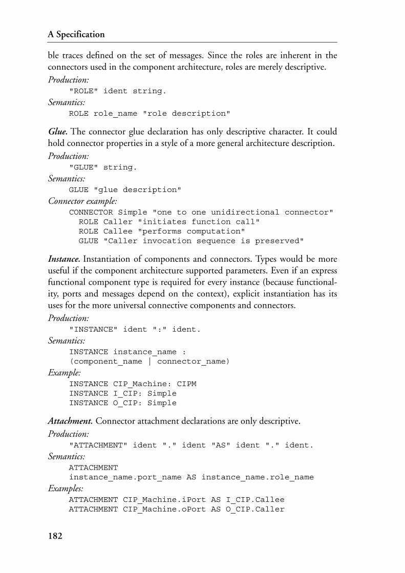
A Specification

ble traces defined on the set of messages. Since the roles are inherent in theconnectors used in the component architecture, roles are merely descriptive.Production:

"ROLE" ident string.

Semantics:ROLE role_name "role description"

Glue. The connector glue declaration has only descriptive character. It couldhold connector properties in a style of a more general architecture description.Production:

"GLUE" string.

Semantics:GLUE "glue description"

Connector example:CONNECTOR Simple "one to one unidirectional connector" ROLE Caller "initiates function call" ROLE Callee "performs computation" GLUE "Caller invocation sequence is preserved"

Instance. Instantiation of components and connectors. Types would be moreuseful if the component architecture supported parameters. Even if an expressfunctional component type is required for every instance (because functional-ity, ports and messages depend on the context), explicit instantiation has itsuses for the more universal connective components and connectors.Production:

"INSTANCE" ident ":" ident.

Semantics:INSTANCE instance_name :(component_name | connector_name)

Example:INSTANCE CIP_Machine: CIPMINSTANCE I_CIP: SimpleINSTANCE O_CIP: Simple

Attachment. Connector attachment declarations are only descriptive.Production:

"ATTACHMENT" ident "." ident "AS" ident "." ident.

Semantics:ATTACHMENTinstance_name.port_name AS instance_name.role_name

Examples:ATTACHMENT CIP_Machine.iPort AS I_CIP.CalleeATTACHMENT CIP_Machine.oPort AS O_CIP.Caller

182

A.2 Input and Output Specification

A.2 Input and Output SpecificationThe purpose of this specification is to arrive at a deterministic and optimizedimplementation from a description that is based on the hardware items on theone hand, and on the input and output signals as used in the functional modelon the other hand. In the running system, input values can be retrieved from avector where each signal is updated periodically according to its timing require-ment and with practically no input jitter. Access macros are provided to guar-antee type integrity. Likewise, output signals are sent using generated macros.

For reasons of optimal utilization it may be advantageous that the resourcesneeded to perform a system’s input and output operations be centralized.Oftentimes, this results in a single such specification for an entire system,although several distinct collections with separate specifications are also possi-ble. Additional data structures are generated that are required for the transmis-sion of input and output data in distributed systems. The choice of a suitablemeans of data forwarding depends on the hardware architecture and the prefer-ences in a specific implementation. Various transmission schemes are sup-ported, such as point-to-point forwarding and broadcast via dedicated links orshared memory.

A.2.1 The Generator ‘acc’

Specification data from a textual input file (defaults to IO.config) is used tocreate the files IO.c (containing the generated code), IO.h (the pertainingheader file), and IO.lst (a summarizing hardware and software configurationdescription for documentation purposes).

Call Syntax:acc [input_file]

A.2.2 Specification Language

The specification language reflects a hardware-oriented view of the system con-figuration. Rather than generate the entire code from an abstract description, itserves as a means of integrating already tested and profiled low-level code rou-tines or macros into the overall structure of a universal input and output sys-tem. This purpose is reflected in the input language, which incorporatesarbitrary function calls including parameters, but does not itself permit thespecification of functionality. Keywords, identifiers and numbers are comple-mented by a set of wildcards that are needed for parameter substitution.

183

A Specification

Keywords:VERSION specification version,SAMPLING sample frequencies,INCLUDE file inclusion,CONSTANT constant definition,INIT initialization,CARRIER carrier board,MODULE mezzanine module,HI, MED, LOW input signal,OUTPUT output signal,PATTERN mask and pattern definition,VOID (reserved).

The syntax permits the use of:

• characters (case sensitive),• numbers in the formats int (1), float (1.0), hexadecimal (0x1),

binary (0b1), int and float can be negative,• function- (or macro-) calls with parameters,• wildcard characters for various automatically substituted parameters:.b carrier board address (base),.s mezzanine module number (slot number 0...3),.c ‘channel setup value’ (for the actual channel),.n ‘channel setup value’ (for the next channel of same device),.hd raw data (hardware data),.sd converted data (software data),.l local static storage,.t temporary storage,.m mask (for binary signals),

• , as divider,• comments (/*...*/) may be used where whitespace is legal.

A.2.3 Productions

The productions are described using the above keywords and the following ter-minal symbols:

ident any valid C identifier,cardinal positive integer number,number number as defined above, at times int required,procedure function call with (actual or wildcard) parameters,string character string delimited with "".

184

A.2 Input and Output Specification

I/O production:Version Sampling {Include | Define | Init} {Carrier}

Version. Defines the specification version in a free format.Production:

"VERSION" string.

Semantics:VERSION version

Example:VERSION "590202"

generates the line#define VERSION "590202"

Sampling. Used to declare the sampling frequencies (in [Hz]). Strictly speak-ing, the relation among the three frequency classes HI, MED, and LOW aredefined. It is the responsibility of the caller in the implementation to match thehighest (or base) sampling rate with the one defined for class HI.Production:

"SAMPLING" cardinal cardinal cardinal.

Semantics:SAMPLING HI_Freq MED_Freq LOW_Freq

Example:SAMPLING 1000 100 10

The sampling frequencies are set to 1 kHz, 100 Hz, and 10 Hz for the fre-quency classes HI, MED, and LOW, respectively (using a base sampling rate of 1 kHz).

Include. Inserts a preprocessor directive (with optional comment).Production:

"INCLUDE" string [string].

Semantics:INCLUDE "file_name.ext" "comment (optional)"

Example:INCLUDE "MLib.h" "mezzanine module definitions"

generates the line#include "MLib.h" /* mezzanine module definitions */

Constant. Preprocessor constant declaration.Production:

"CONSTANT" ident number [string].

Semantics:CONSTANT const_name const_value "comment (optional)"

185

A Specification

Example:CONSTANT OCmA_MAX 0x800 "max. value for ICX outputs"

generates the line#define OCmA_MAX 0x800 /* max. value for ICX outputs */

Init. Declaration of initialization function calls for global settings as well as forindividual carrier boards and single modules.Production:

"INIT" procedure {procedure}.

Semantics:INIT Init_fct_1(p1,p2,..) Init_fct_2(p1,p2,..) ..

Example:INIT vme_address_modifier(0x3d)

A call to this function will be inserted into the system initialization function IO_Init(). The statement may be followed by an arbitrary number of other initialization calls.

Carrier. Declares a carrier board and its base address. Carrier board declara-tions can also be used for declarations concerning cards with their own func-tionality, i.e., additional mezzanine module components are optional. When acarrier does not contain any modules, its own functionality is optional.Production:

"CARRIER" ident number [string] {Module}{(Input {Pattern}) | (Output {Pattern)}.

Semantics:CARRIER name base_address "comment (optional)" MODULE .. HI .. PATTERN .. OUTPUT .. PATTERN ..

Example:CARRIER R__VA26 0xaaa800 "this card is a joker" MODULE

This declares the carrier board R__VA26 having base address 0xaaa800, together with the given comment.

Module. Declares a mezzanine module including its position on the carrierboard (slot 0…3). Modules are related to the specific carrier board that pre-cedes the module declaration. A single module may offer both input and out-put functions.Production:

"MODULE" ident cardinal [string].

Semantics:MODULE name slot "comment (optional)"

186

A.2 Input and Output Specification

Example:MODULE R__M331 0 "16ch AD mezzanine module" MED ..

This declares the mezzanine module R__M331, in slot 0 on its carrier.

HI, MED, LOW (Input). Input signal acquisition can be a lengthy process thatdepends on the kind of signal and especially on the peripheral hardware itemsinvolved. To cater for the majority of possible combinations, signal inputs aredefined as sequential processes like in Fig. 119. Some of the stages are optional.

Figure 119: Input phases

Inputs are qualified by their frequency class and by the following information:

Production:"input class" ident cardinal number procedure, cardinal, cardinal procedure, cardinal procedure procedure.

Semantics:( HI | MED | LOW ) name simline ch_setup I_Setup_fct(..), T_setup, T_wait I_Acc_fct(..), T_acc I_Conv_fct(..) I_Check_fct(..)

Example:HI ICmP03 22 101 M34_st_set_mode(.b,.s,.n),3,7 M34_rd(.b,.s,.hd),3 I_F(.sd,.hd,0.000488,-0.4) VOID

Table 4: Input configuration items

signal name

simulation model interface vector index

setup value

setup function call, with execution time and delay time [µs]

access function call, with execution time [µs]

conversion function call

check function call

setupaccess convert check

187

A Specification

This specification describes an input signal of class HI with initialization value 101 and the three setup, access, and conversion function calls. The keyword VOID indicates an empty check function. Function parameters are either constants or wildcard characters that will later be substituted by the generator. The execution and delay times needed in generating the access schedule must be known beforehand for all functions (i.e., determined by profile measurements). In a simulation implementation, this input signal would be connected with the simulating environment via vector item 22.

Output. Similar to the sequence defined for data acquisition, outputs are seenas consisting of at most three separate stages, all of which are optional but forthe access call itself.

Figure 120: Output phases

To declare an output signal, the following information is required:

Production:"OUTPUT" ident cardinal number procedure procedure, cardinal, cardinal procedure, cardinal.

Semantics:OUTPUT name simline ch_setup O_Conv_fct(..) O_Setup_fct(..), T_setup, T_wait O_Acc_fct(..), T_acc

Example:OUTPUT O__A04 14 5 B_I(.hd,.sd) VOID ID_M33_wr_data(.b,.s,.c,.hd),3

Table 5: Output configuration items

signal name

simulation model interface vector index

setup value

conversion function call

setup function call, with execution time and delay time [µs]

access function call, with execution time [µs]

convertsetup

access

188

A.3 Event Extraction Specification

This describes an output signal with initialization value 5 and the necessary conversion and access function calls. The setup function is empty. In a simu-lation, the signal would be connected via vector item 14.

Pattern. Patterns, together with the related masks, belong to a specific binaryinput or output signal. The mask name (and its value) is followed by an arbi-trary number of pattern names with their values. The mask name will also beused as a prefix to create the final names for the patterns.Production:

"PATTERN" ident number cardinal {cardinal}ident number {ident number}.

Semantics:PATTERN prefix mask_value simline(s)pattern1 value1 pattern2 value2 ..

Example:PATTERN OHaW1 0x0003 4 5off 0 close 0x0001 open 0x0002

The mask OHaW1_MASK is defined including the patterns OHaW1_off, OHaW1_close, and OHaW1_open. Since two bits are set in the mask, two simulation interface lines must be specified (4, 5), higher order bits first.

A.3 Event Extraction SpecificationEach working node in a distributed system (or the sole one in a single processorinstallation) possesses its own event extractor mechanism. This specificationhas the advantage of preserving the close relation of event messages and theirnames to a node’s functional model. It dissociates the node in question fromthe entire project and makes it easier to adjust to local changes. This is espe-cially rewarding when different teams work with partial installations on theirown test beds. Besides, many events are only of use for a specific node, andbroadcasting them would encumber communication channels unnecessarily.

A.3.1 The Generator ‘evt’

Configuration data from a textual input file (defaults to event.config) isused to generate the header file event.h. This header file needs informationfrom and works only in conjunction with the files IO.c and IO.h that areunique for a system (see section A.2.1).

Call Syntax:evt [input_file]

189

A Specification

A.3.2 Specification Language

The specification language includes a number of keywords to select a node’slocal properties, as for example the resolution of the local delay timers and thepresence of slave nodes. The bulk of a specification centers around the eventsthemselves. The generator is used to translate this information into standard-ized data tables that will be used by optimized routines in an implementation.Not only does generation of these data permit the enforcement of importantdata properties that would otherwise have to be checked at run-time, it alsooffers the advantage of a convenient and intuitive input format.

Keywords:VERSION specification version,NODE node identifier,TTICK the node’s basic timer tick,DISPLAY switch to enable a node’s display features,SLAVE switch for nodes with a plain slave,RSLAVE switch for nodes with a ring slave,BEVENT specifies a discrete (binary) event,CEVENT specifies an event contained within a continuous signal,VOID (reserved).

The syntax permits the use of:

• characters (case sensitive),

• numbers in the formats int (1), float (1.0), hexadecimal (0x1), binary (0b1), int and float can be negative,

• signal names (as used in the input/output specification),

• channel (or process) identifiers,

• event identifiers.

A.3.3 Productions

The productions are described using the above keywords and the following ter-minal symbols:

ident any valid C identifier,cardinal positive integer number,number number as defined above, at times int is required.

Event production:Version Node Timer [Display] [Slave] {BEvent | CEvent}

190

A.3 Event Extraction Specification

Version. Defines the specification version in a free format.Production:

"VERSION" string.

Semantics:VERSION version

Example:VERSION "521101"

generates the line#define VERSION "521101"

Node. This production is used to identify the node that the current event spec-ification belongs to. In an implementation, local timers will be initialized witha random number based on this identifier to prevent the accumulation ofexpiring timers throughout the entire system. Additionally, identifiers are cre-ated by which the node is individualized in the global scope.Production:

"NODE" ident.

Semantics:NODE name

Example:NODE CC

The node’s identity is CC, which gives rise to the following definitions:#define NODEID CC#define _SAMPLER _SMP_CC /* this node’s sampler proc */

Timer. Creates a constant needed for the initialization of the local timer inter-val counter. Delay timer ranges used in the functional model directly dependon this value, which unfortunately is implementation-dependent. With a basictimer tick interval of 64 µs, for example, the following values apply:

Production:"TTICK" cardinal.

Semantics:TTICK interval

Example:TTICK 3125

Table 6: Delay timer values

3125 ≈ 0.2 s

625 ≈ 0.04 s

125 ≈ 0.008 s etc.

191

A Specification

Display. The presence of this keyword indicates that the node uses global dis-play features1, in which case the required code fragments for communicatingwith the display node are inserted. This production applies only to distributedsystems.Production:

"DISPLAY".

Semantics:DISPLAY

Slave. These keywords indicate if a node possesses additional private (SLAVE)or public (RSLAVE) slave nodes. If either keyword is present, code fragmentsfor private or public communication with the slave node(s) will be provided,respectively. This production applies only to distributed systems.Production:

"SLAVE" | "RSLAVE".

Semantics:SLAVE | RSLAVE

BEvent. Events from binary input data are raised when ever the input haschanged and one of the defined patterns (see p. 189) is recognized in the inputdata. This production establishes a connection between patterns and eventmessages that are understood by the functional model. Aside from the signaland event identifiers, a channel is specified. This channel’s message alphabetmust contain the used event messages.Production:

"BEVENT" ident ident (ident ident {ident ident}).

Semantics:BEVENT Signal_ID Channel_ID (Event Value {Event Value})

Example:BEVENT ICoP01 Evt_Chan (P_rises ICoP01_normal P_sinks ICoP01_low)

Entries in two tables will be generated. The first one is the binary event con-trol table containing references to the input signal, message channel, and binary event data table, as well as the signal mask ICoP01_MASK, the num-ber of defined events and a variable field where the value that was last seen will be stored. The binary event data table contains the events themselves and their associated patterns.

1. Another tool (dsp), which is not described here, is used for specifying a system’s display function-ality. It is based on the notion of an arbitrary number of screens that are populated by instruments taken from a toolbox. The specification contains display properties, such as display formats, refresh rates, warning thresholds etc. Implementations are also created by a code generator.

192

A.4 Code Generator Program Structure

CEvent. The occurrence of events depending on quasi-continuous input data isrelated to threshold values. These thresholds can be set within the entire signalrange, although they must conform to certain conditions:

• the way the event extractor algorithm is implemented requires a hysteresis. Therefore, two signal values must be specified for each threshold,

• thresholds must be given in ascending order,

• even in the case where only one transition will give rise to an event, both val-ues are mandatory! In these cases, the keyword VOID replaces a valid event name.

Production:"CEVENT" ident ident (ident number ident number {ident number ident number}).

Semantics:CEVENT Signal_ID Channel_ID (DownEvent DownValue UpEvent UpValue {DownEvent DownValue UpEvent UpValue})

Example:CEVENT ICmT03 Evt_Chan (freeze -0.1 dew 0.1 condense 99.0 evaporate 101.0)

As for binary events, entries in two tables will be generated. The first is the continuous event control table (allegedly a slight misnomer…) with refer-ences to the input signal, message channel, and continuous event data table. This last pointer will be updated during operation to reflect the range where the signal is currently in. The continuous event data table contains an ordered list of events and their associated threshold values. The lower and upper limits are marked with -FLT_MAX, FLT_MAX, respectively, allowing for an efficient implementation of the extractor algorithm.

A.4 Code Generator Program StructureAll the generators are built along the same lines, even sharing some of the mod-ules. As an example, the structure of the program acc is presented in moredetail (Fig. 121). It consists of five modules:

• the scanner (scanner.c, scanner.h), extracts tokens from character sequences and emits error messages while reading the input file,

• the parser (parser.c), performs syntactic analysis and inserts read data into the symbol, access procedure and initialization tables,

• the input access distribution scheduler (schedule.c), computes the static schedule for data input, taking into account the different frequency classes,

193

A Specification

• the module data (data.c, data.h), manages static data; moreover, data.h contains all global definitions and declarations,

• the file generator (access.c), performs final parameter substitutions and generates the output file; it also contains the main program.

Figure 121: Code generator program structure (acc)

A.4.1 Data Structures

Symbol Table. The symbol table contains all addresses, constants, signals,masks, and patterns. The item types correspond to the elements indicated bykeywords in the specification language.

S_HEADER first element (empty)S_INCLUDE include fileS_CONST constantS_CARRIER module carrier boardS_MODULE mezzanine moduleS_CHAN signalS_MASK mask (of a binary signal)S_PATTERN pattern (belongs to a mask)

It is implemented as a list of lists with elements defined as follows:

Table 7: ST (symbol table) data fields

Field name Description

char *name symbol name

char *rem remark or comment

int a,b,c,d symbol data

int type symbol type

struct ST *up pointer to parent symbol

struct ST *dwn pointer to child symbol (list)

struct ST *next pointer to other symbols of the same type

ACCESS

SCANNER

PARSER

DATA

SCHEDULE

194

A.4 Code Generator Program Structure

Depending on the symbol table type, data fields a...d are used in specificways, and they may also be empty. Items in parentheses are optional, their usedepends on the signal type:

Example Specification. The configuration in Fig. 122 contains three mezzaninemodules (M342, M331, and M313) on two different carrier boards (R__VA28,R__VA2A). IElI01, IElI02, IElI03, and OElA05 are continuous input oroutput signals, respectively, and ICoP1, IElC2 are binary input signals includ-ing their masks ICoP1_MASK, IElC2_MASK and the patterns ICoP1_high,ICoP1_low, and IElC2_ON, respectively. The internal representation of thissetup is shown in Fig. 123.

Figure 122: Example signal configuration

Table 8: ST (symbol table) data field usage

type a b c d

S_HEADER

S_INCLUDE

S_CONST const value

S_CARRIER address card number

S_MODULE slot number slot id

S_CHAN max_hi_cnt idx -1 HI (I_Hist[]idx)

-1 max_i_cnt idx MED, LOW (I_Hist[]idx)

O_Acc index O_Bin[] idx OUTPUT

S_MASK mask value HI, MED, LOW I_Val.value[]idx

mask value OUTPUT O_ConvSend idxO_Acc idx

S_PATTERN pattern value

R__VA28

R__VA2A

OElA05

IElI01

IElI02

IElI03

ICoP1

IElC2

M313

M342

M331

Carrier Module Signal

ICoP1_MASKICoP1_high

ICoP1_low

IElC2_MASK IElC2_ON

Mask Pattern

195

A Specification

Figure 123: Internal signal representation

S_HEADER

S_CARRIER

S_MODULE

S_MODULE

S_CHAN

S_CHAN

S_CHAN

S_MASK

S_CARRIER S_CARRIER

R__VA28 R__VA2A

S_MODULE

S_MODULE

S_MODULE

S_CHAN S_CHAN S_CHAN

S_CHAN

S_CHAN S_CHAN

S_MASK S_MASK

S_PATTERN S_PATTERN S_PATTERN

S_PATTERN S_PATTERN

M342 M331

M313

IElI01 IElI03IElI02

OElA05

IC0P1 IElC2

IC0P1_MASK IElC2_MASK

IC0P1_high IC0P1_low

IElC2_ON

type

name

up nextdwn

196

A.4 Code Generator Program Structure

A.4.2 APs (Access Procedures)

An access procedure item (AP) contains all information needed to perform theactual bus accesses:

The entry mask is only used for binary data and points to the pertaining mask,next is used for channels that need more than one access procedure per signal,e.g., all binary modules with several masks.

The AP elements are accessible through lists for each signal class (APLs).

The first element in the list remains empty at all times; new elements areattached at the end of the list, pointed to by APL_Last[]. There are four lists:

Table 9: AP (access procedure) data fields

Field name Description

char *setup setup call

char *access access call

char *conv conversion call

char *test data check/test call

int flag essential

int s setup time

int d delay time

int a access time

int setup_val setup value

S_Ptr channel pointer to the channel in the symbol table

S_Ptr mask pointer to the mask in the symbol table

AP_Ptr next pointer to the next AP, if several APs are to execute in a sequence

Table 10: APL (access procedure list) list element

Field name Description

AP_Ptr p pointer to an AP

APL_Ptr next pointer to the next list item

Table 11: APL (access procedure list) lists

Variable Description

APL_Base[HI] APs of frequency class HI

APL_Base[MED] APs of frequency class MED

APL_Base[LOW] APs of frequency class LOW

APL_Base[OUTPUT] OUTPUT type APs

197

A Specification

A.4.3 IPs (Initialization Procedures)

IPs contain initialization functions that are stored in a linked list. An IP ele-ment consists of four fields:

The elements are stored in the same sequence they are encountered, i.e., thefirst initialization function read from the specification file will be executed first.

A.4.4 Variables

Freq. Frequencies are given in Hertz. Freq is of type int Freq[3].

Indices and Vector dimensions. A collection of variables containing the actualindices for the next element of various vectors. Upon completion of the syntac-tic analysis, these values correspond with the respective vector sizes for use inthe generated files.

max_i_hist_cnt,/* I_Hist[] index count max value */max_hi_cnt, /* BC_S_Data.value[] (HI) index count max value */max_i_cnt, /* BC_R_Data.value[] (MED/LOW) index max value */max_o_bin_cnt, /* O_Bin[] index count max value */max_o_cv_cnt; /* O_ConvSend[], O_Acc[] index count max value */

max_hw_cnt, /* I_HW_Vec[] index count max value */max_ml_cnt; /* .ML_x[] index item count max value */

S_Actual. S_Actual contains the actual (i.e., the one that was accessed last)symbol in the symbol table.

S_Actual, /* last (actual) accessed symbol */S_actCarrier, /* current carrier record */S_actModule, /* current module record */S_actMask, /* current mask */S_actPattern; /* current pattern */

Table 12: IP (initialization procedure) list element

Field name Description

char *routine initialization function call

int value initialization value

S_Ptr module pointer to module (used for ‘private’ initializations)

struct IP *next next IP

Table 13: Sampling frequencies

Variable Description

Freq[HI] Sampling frequency for type HI signals

Freq[MED] Sampling frequency for type MED signals

Freq[LOW] Sampling frequency for type LOW signals

198

A.4 Code Generator Program Structure

A.4.5 Access Distribution

Access distribution is performed in two stages. First, all signals that must beread in the i-th sampling period are selected and stored in the variable slice.Then the required accesses are combined with permutations and the best com-bination is chosen.

Selection of the Signals for One Period. A number of signals from frequencyclasses MED and LOW must be selected in each sample period that are to be readalongside the signals of class HI. The selection is crucial in order to achieve aneven distribution of all accesses, i.e., if there are 10 such signals and 10 periods,one is read in each period (as opposed to reading all ten in a single period). Thealgorithm can be outlined as follows.

The total number of signals as well as the required sampling fre-quencies are known from parsing. The signals of class HI are readin every period, MED signals only every periods,and the signals of class LOW are read only every periods. The objective is to obtain an even distribution of all accesses throughsampling periods to . The total number of signals that must be accessedper period amounts to (a remainder is possible).

In the hardware-oriented configuration input file, the signals are orderedaccording to their location on carrier cards and module slots. Because exclusionrelations between signals on the same slot, i.e., the same mezzanine card arehighly probable, signals are not inserted into the schedule in the same sequenceas they are encountered in the configuration. By following this strategy mostsituations where two signals belonging to the same hardware item end up inthe same sample period can be avoided from the start, thus reducing the num-ber of conflicts that must be resolved later.

A signal of type is read in every th period. Specialcare must be taken to accommodate the possibly remaining signals. The array

holds values between and . Anadditional signal is copied, if . This technique hasthe disadvantage of accumulating a remaining signal of each class MED and LOWin the last scheduler period, which is detrimental to the distribution algorithm(an optimized permutation, see Access Distribution, below). The efficiency ofthis algorithm may depend on the presence or absence of a single additionalsignal. The problem is solved in the generator by explicitly altering the contentsof in such a way that the remaining signals of class LOW areinserted into those slices where signals of class MED will be inserted with a verylow probability only.

Total class[ ]Freq class[ ]

m Freq HI[ ] Freq MED[ ]⁄=l Freq HI[ ] Freq LOW[ ]⁄=

0 l 1–elem class[ ] Total class[ ] Freq class[ ]⋅ Freq HI[ ]⁄=

class Freq HI[ ] Freq class[ ]⁄

counter class[ ] 0 Freq HI[ ] Freq class[ ]⁄( ) 1–rest class[ ] counter class[ ]>

counter class[ ]

199

A Specification

Variables and Procedures. The signals that must be dealt with in a specificperiod are contained in variable Slice.

APL_Ptr Slice;

Slice is a list of pointers to APs. The first element in a slice is always empty. Anumber of procedures facilitate the administration and the use of slices:

Slice_Init()

must be called to initialize a slice and all connected structures.

Slice_New()

generates the next slice.

Slice_next_AP()

searches for the next free element in a slice. Elements whose slots have beenallocated to another signal are skipped. One of three search methods is chosenwith a parameter:

• search next element, starting at the actual position,

• search next element, starting at the beginning,

• search next element from the actual position to the end of the list (no reset at the end).

Access Distribution. The best distribution of all accesses can be found bysearching through all permutations. Unfortunately, there exists no feasibleinductive way to achieve this.

A reasonable distribution can be accomplished in with a simple heuris-tics. First, the dependencies between different accesses are represented in adirected acyclic graph. The only dependencies to account for are possible accessclashes to the same module within a single slice. In order to catch these con-flicts, it is therefore sufficient to create a list of accesses for each module. First,the variable w.start that indicates the earliest possible start time is initializedto 0 for all the first elements in a slice, along with the slice timer time. Thenthe PathCycles for each element in a serial schedule are calculated, i.e., thetime (in ms) remaining until the end of the schedule is reached. The scheduleitself is then obtained with the following algorithm:

1. time= 02. WHILE (not all elements inserted)2.1 IF (there exist elements with w.start <= time)2.2 THEN take element w with highest number of PathCycles2.3 ELSE take element w with lowest start time2.4 insert element w into the global schedule2.5 w.start= MAX(w.start, time)2.6 time= w.start + w.wait2.7 w.next.start= w.start + w.wait + w.delay

O n2( )

200

A.4 Code Generator Program Structure

The heuristics is to be found in lines 2.1 to 2.3. A signal w is chosen (2.2)whose first access is executable immediately (start <= time) and which needsthe most accesses to complete, i.e., the one that will cause the greatest numberof gaps in the form of delay time between individual accesses. The earlier it isinserted, the easier it will be to fill the gaps. If there is no such signal left (2.3),then the signal that produces the smallest gap is chosen. Because its next accesscannot be scheduled directly, a delay instruction of duration w.start-timemust be inserted to satisfy 2.5. In 2.6, the slice time is updated to after theexecution of w has completed, and 2.7 calculates the start time for the nextinstruction.

201

A Specification

202

B Syntax

B.1 ArchitectureSCANNER pvt;

CHARACTERSeofC = {0X}.blankC = {020X} | {09X} | {0DX}.any = {0X..0FFX} - eofC.letter = {"A".."Z","a".."z"}.digit = {"0".."9"}.binary = {"0","1"}.hex = digit + {"a".."f","A".."F"}.

TOKENSeof = eofC.void = "VOID".ident = (letter | "_") {letter | digit | "_"}.cardinal = digit {digit}.number = (["-"] digit {digit} ["." {digit}]) |

("0X" | "0x") hex {hex} |("0B" | "0b") binary {binary}.

string = "" {any} "".stdtype = "void" | [signed | unsigned]

"char" | "short" | "int" | "long" | "float" | "double").

COMMENT FROM "/*" TO "*/" UNNESTED

LITERALS"VERSION", "CONSTANT", "TYPE", "INIT","COMPONENT", "PORT", "IN", "OUT", "MESSAGE", "COMPUTATION","CONNECTOR", "ROLE", "SOURCE", "SINK", "GLUE","INSTANCE", "ATTACHMENT",",", ";", "(", ")", "[", "]", "&", "|", "=", "!"

END pvt.

GRAMMAR pvt;

SKIP blankC;

Pivot = Version {Constant | Type | Component | Connector} {Instance}.

Version = "VERSION" string.

203

B Syntax

Constant = "CONSTANT" ident number [string].

Type = "TYPE" (Scalartype | Recordtype | Arraytype).

Scalartype = (ident | stdtype) ident [string].

Recordtype = ("struct" | "union") [ident] [string]"{" {([("struct" | "union")] ident | stdtype)ident {"," ident} ";"} "}" ident.

Arraytype = (ident | stdtype) ident"[" (number | ident) {"," (number | ident)} "]" [string].

Init = "INIT" procedure {procedure}.

Component = "COMPONENT" ident [string] {Port} Computation.

Port = "PORT" ("IN" | "OUT") ident [string] {Message}.

Message = "MESSAGE" ident ((ident ident "(" ident {"," ident} ")")| void) [string].

Computation = "COMPUTATION" ident [string].

Connector = "CONNECTOR" ident [string] {Role} Glue.

Role = "ROLE" ident string.

Glue = "GLUE" string.

Instance = "INSTANCE" ident ":" ident.

Attachment = "ATTACHMENT" ident "." ident "AS" ident "." ident.

END pvt.

B.2 Input and OutputSCANNER acc;

CHARACTERSeofC = {0X}.blankC = {020X} | {09X} | {0DX}.any = {0X..0FFX} - eofC.letter = {"A".."Z","a".."z"}.digit = {"0".."9"}.binary = {"0","1"}.hex = digit + {"a".."f","A".."F"}.

TOKENSeof = eofC.void = "VOID".ident = (letter | "_") {letter | digit | "_"}.cardinal = digit {digit}.number = (["-"] digit {digit} ["." {digit}]) |

("0X" | "0x") hex {hex} |("0B" | "0b") binary {binary}.

string = "" {any} "".wildcard = ".b" | ".s" | ".c" | ".n" | ".hd" | ".sd" | ".l" | ".t" | ".m".procedure = ident "(" [(ident | wildcard) {"," (ident | wildcard)}] ")".

COMMENT FROM "/*" TO "*/" UNNESTED

204

B.3 Event

LITERALS"VERSION", "SAMPLING", "INCLUDE", "DEFINE", "INIT", "CARRIER", "MODULE","HI", "MED", "LOW", "OUTPUT", "PATTERN",",", ";", "(", ")", "[", "]", "&", "|", "=", "!"

END acc.

GRAMMAR acc;

SKIP blankC;

IO_Config = Version Sampling {Include | Define | Init} {Carrier}.

Version = "VERSION" string.

Sampling = "SAMPLING" cardinal cardinal cardinal.

Include = "INCLUDE" string [string].

Define = "DEFINE" ident number [string].

Init = "INIT" procedure {procedure}.

Carrier = "CARRIER" ident number [string] {Module}.

Module = "MODULE" ident cardinal [string]{(Input {Pattern}) | (Output {Pattern)}.

Input = ("HI" | "MED" | "LOW") ident cardinal number((procedure "," cardinal "," cardinal) | void)((procedure "," cardinal) | void)(procedure | void)(procedure | void).

Output = "OUTPUT" ident cardinal number (procedure | void) ((procedure "," cardinal "," cardinal) | void) ((procedure "," cardinal) | void).

Pattern = "PATTERN" ident number cardinal {cardinal} ident number {ident number}.

END acc.

B.3 EventSCANNER evt;

CHARACTERSeofC = {0X}.blankC = {020X} | {09X} | {0DX}.any = {0X..0FFX} - eofC.letter = {"A".."Z","a".."z"}.digit = {"0".."9"}.binary = {"0","1"}.hex = digit + {"a".."f","A".."F"}.

TOKENSeof = eofC.void = "VOID".

205

B Syntax

ident = (letter | "_") {letter | digit | "_"}.cardinal = digit {digit}.number = ["-"] digit {digit} ["." {digit}] |

("0X" | "0x") hex {hex} |("0B" | "0b") binary {binary}.

string = "" {any} "".

COMMENT FROM "/*" TO "*/" UNNESTED

LITERALS"VERSION", "NODE", "TTICK", "DISPLAY", "SLAVE", "RSLAVE","BEVENT", "CEVENT", ",", ";", "(", ")", "[", "]", "&", "|", "=", "!"

END evt.

GRAMMAR evt;

SKIP blankC;

Evt_Config = Version Node Timer [Display] [Slave] {BEvent | CEvent}.

Version = "VERSION" string.

Node = "NODE" ident.

Timer = "TTICK" cardinal.

Display "DISPLAY".

Slave = "SLAVE" | "RSLAVE".

BEvent = "BEVENT" ident ident (ident ident {ident ident}).

CEvent = "CEVENT" ident ident(ident number ident number {ident number ident number}).

END evt.

206

C Glossary

Accuracy. The systematic (repeatable) error in a measurement (→ precision).

Accuracy interval. The maximum permitted time interval between the point of observation of a controlled pro-cess and the point of use of the corresponding measured data.

Action. Any activity aimed at bringing about an effect. Specifically, an action is the output of a CIP transition that eventually affects the controlled processs in the environment.

Active task. Refers to the task that is currently running. Multi-tasking operating systems need to know the iden-tity of the currently running task in order to save its context in the right place when it is suspended.

Actuator. A transducer that accepts data and trigger information from an interface node and realizes an intended effect in the controlled process.

Address bus. A set of electrical lines connected to the processor and all of the peripherals with which it com-municates. The address bus is used by the processor to select a specific memory location or register within a particular peripheral. If the address bus contains n electrical lines, the processor can uniquely address up to 2n such locations (→ data bus).

Alarm shower. A correlated set of alarms that is caused by a single primary event.

Aliasing. The process where a sinusoid is perceived at a frequency different from its original frequency as a result of sampling or another nonlinear action (→ anti-alias filter).

Anti-alias filter. Low-pass filter placed before an analog-to-digital converter. The filter removes frequencies above the sampling rate that would alias during conversion (→ aliasing).

Aperiodic task. A task where neither the task request times are known nor the minimum time interval between successive requests for execution (→ periodic task, sporadic task).

API. Application program interface. The data and control interface between an application program and the operating system.

Application software. All the software modules specific to a particular embedded project.

Application specific fault tolerance. Fault tolerance mechanisms that are introduced within the application code (→ systematic fault tolerance).

A priori knowledge. Knowledge about the future behavior of a system that is available ahead of time.

Architecture. The description of a system’s constituents and their interrelations. Either the abstract description of functional components and their interconnection (operational architecture), or the hardware compo-nents used to build a system, and their interconnections (implementation architecture).

ASIC. Application specific integrated circuit. A special-purpose circuit that is used to implement certain parts of a system’s functionality directly, without any underlying general-purpose computation engine.

Assembler. A software development tool that translates human-readable assembly language programs into machine language instructions that the processor can understand and execute.

Assembly language. A low-level human-readable form of a processor’s instruction set.

Assertion. A predicate or a set of conditions that must be satisfied at a particular point during program execu-tion.

1 2⁄

207

C Glossary

Assumption coverage. The probability that assumptions made in the model building process hold in reality. The assumption coverage limits the probability that conclusions derived from a model will be valid in the real world.

ATM. Asynchronous transfer mode. An asynchronous communication technology for communication over broadband networks where the information is organized into constant length cells (48 data bytes, 5 header bytes).

Atomic data structure. A data structure that has to be interpreted as a whole.

Atomic operation. An operation that has the all-or-nothing property. It either completes and delivers the intended result or else does not have any effect.

Availability. A measure of the correct service delivery regarding the alternation of correct and incorrect service, measured by the fraction of time that the system is ready to provide the service.

Backbone network. A non real-time communication network for the exchange of non time-critical information between a real-time computer system and the data-processing systems of an organization.

Back-pressure flow control. In back-pressure flow control, the receiver of a sequence of messages exerts back pressure on the sender so that the sender will not outpace the receiver.

Bandwidth. The maximum number of bits that can be transmitted across a channel per time unit.

Behavior. A functional and temporal description of how a system is expected to execute.

Bit dominance. A communication protocol based on bit-wise arbitration. On bus idle, all competing nodes start to transmit their unique node identification value simultaneously, while continuously monitoring the signals present on the bus. Contention is resolved by the transmission medium where low signals override high signals (or vice versa). If a node detects a dominant signal opposite to its own, it drops out of the competition. Throughput and efficiency are high (because the arbitration is part of the message), the protocol is robust (because no specific transmission order is required). Fairness can be a problem under heavily loaded conditions. This protocol is used in CAN.

Bit-length of a channel. The number of bits that can traverse the channel within one propagation delay.

Blocking. When the execution of a task is suspended because of another task. Causes are manifold: it may attempt to acquire a semaphore that is unavailable, or when it waits for a message that is not in its queue, or while it waits for a pause to expire, or when, in a time-slicing system, its time-slice has expired, to give a few examples.

BNF. Backus-Naur form. A meta language to describe syntactic properties of computer languages [Wir77]. Repetition is denoted by {} (i.e., {a} stands for ε | a | aa | aaa | …), optionality by [] (i.e., [a] stands for ε | a). Terminal symbols are enclosed in "" (a quote mark as a literal is written twice).

Broadcast. A communication scheme where all nodes aside from the sender are receivers.

Busy waiting. → polling.

Byzantine error. Occurs if a set of receivers receive different (conflicting) values about a controlled process at some point in time. Some or all of these values are incorrect (synonym. malicious error).

C. Common programming language used in science end engineering [KeR88, Joy96].

CAN. Controller area network. A low-cost event-triggered real-time communication network that is based on the bit dominance protocol. The serial bus has multi-master capabilities and handles simultaneous requests through non-destructive bit-wise arbitration, guaranteeing low latency to the highest priority message.

Causal order. A causal order among a set of events is an order that reflects the cause effect relationships between the events.

Channel access delay. The time between the request for sending a message and the start of its transmission.

CIP. Communicating interacting processes. A method and corresponding graphic tool for modeling the func-tional part of an embedded system, based on extended FSMs (→ system, cluster, process).

Clock. A device for time measurement that contains a counter and a physical oscillation mechanism that peri-odically generates an event to increase the counter.

Cluster. A cluster embraces a number of synchronous processes as part of a CIP system. Clusters are asynchro-nous among themselves.

CNI. Communication network interface. The interface between the communication controller and the host within a node of a distributed computer system.

208

C Glossary

Communication. The activity of receiving and transmitting information. In a CIP system, communication is asynchronous across the boundaries of a node using messages (→ interaction).

Communication controller. One or several communication controllers control the communication of a node within a distributed computer system.

Compiler. A software development tool that translates high-level language programs into the machine-lan-guage instructions that a particular processor can understand and execute.

Composability. An architecture is composable regarding a specified property if the system integration will not invalidate this property, provided it has been established at the subsystem level.

Computational resource. A time-shared, preemptable component, or group of components, in the hardware architecture.

Congestion. If the demand for network resources exceeds the available capacity over some period of time, a net-work is said to be congested. Congestion leads to high jitter and packet loss, which can also be thought of as infinite delay variation.

Connection configuration. A high level description of a real-time computer system’s connective elements, i.e., all the aspects concerned with its embedding and not related to its functional model.

Connection Oriented Protocol. A protocol with only two nodes per physical transmission medium, typically connected with serial lines. Its behavior is deterministic between directly connected nodes, whereas latency can be high for indirect connections.

Construction. The bottom-up activity of actually building a system in accordance with a design.

Contact bounce. The random oscillation of a mechanical contact immediately after closing.

Contention. Competition for resources. Used in networks to describe the situation where two or more nodes attempt to transmit a message at the same time (→ CSMA, controlled access).

Context. The current state of the processor’s registers and flags. In a more complete sense context also includes the task’s local variables and its subroutine nesting information.

Context switch. The process of suspending one task in favor of another one in a multi-tasking system. A context switch involves saving the context of the running task and restoring the previously-saved context of the other. The code that does this is necessarily processor-specific.

Continuous signal. A signal that is formed from continuous variables, such as a voltage varying with time (synonym. analog signal, → discrete signal).

Control. The purposeful influencing of a controlled process’s signals in combination with information process-ing. In closed-loop control, an object’s controlled variable is continuously monitored and its input sig-nals adjusted, so that it corresponds to a reference variable. In contrast, open loop control has no feedback; an object’s output signals are merely influenced according to the inner laws of this object.

Controlled access. A technique that avoids contention by deliberately limiting access to resources (→ TDMA).

Controlled process. The object in the environment that is to be controlled by the real-time computer system, such as an industrial plant, or a device.

Control system. Any contrivance that performs control functions within an environment with which it is usu-ally tightly integrated. With the advance of digital computers, embedded system is increasingly becoming a synonym for control system.

Cooperative scheduling. Each in a group of cooperative scheduling tasks voluntarily relinquishes control so that other tasks can run. If control is not given up deliberately other tasks will be starved. Control can be relinquished explicitly by a yield, pause, or suspend, or implicitly by waiting for an event (→ priority based preemptive scheduling, time-sliced scheduling).

CORBA. Common object request broker architecture. Enables pieces of programs, called objects, to commu-nicate with one another regardless of what programming language they were written in or what operat-ing system they are running on [OMG95].

CPU. Central processing unit. The part of a processor that executes instructions.

CRC. Cyclic redundancy check field. An extra field in a message for the purpose of detection of value errors.

Critical section. A block of code that must be executed in sequence and without interruption to guarantee correct operation of the software.

Cross-compiler. A compiler that runs on a different platform than the one for which it produces object code. A cross-compiler runs on a host computer and produces object code for the target.

209

C Glossary

CSMA. Carrier sense multiple access protocol. A set of rules determining how network devices respond when two devices attempt to use a physical medium simultaneously. Collisions are detected and resolved with exponential back off (CD, Ethernet), or avoided by generating contention slots following a collision (CA). The protocol’s key advantage is its ability to accommodate an unlimited number of nodes with-out requiring network initialization and configuration. However, under heavy traffic the overhead is unbounded due to repeated collisions, lowering determinacy and efficiency. CSMA is a type of conten-tion protocol.

CSP. Communicating sequential processes. A formal method where systems are described as a number of com-ponents (processes) that operate independently and communicate with each other over well-defined channels. This basic (synchronous) communication model is one of the core ideas underlying the occam programming language.

Cyclical scheduling. Accomplished by simply calling one task after another in an infinite loop. The advantages are that it is small and easy to understand and control, that it does not require a complicated operating system and only one stack. The disadvantages are missing priorities, that tasks must retain their states between runs, and the possibility of excessive loop latency when there are many tasks (synonym. round robin scheduling).

Data bus. A set of electrical lines connected to the processor and all of the peripherals with which it communi-cates. When the processor wants to read/write the contents of a memory location or register within a particular peripheral, it sets the address bus pins appropriately and receives/transmits the contents on the data bus.

Data encoding technique. Defines the way in which the logical bits are translated into physical signals on the transmission medium. Usually, through a redundant format, measures are taken to ease clock extraction and to remove DC components.

Deadline. The point in time when a result should/must be produced (→ soft deadline, hard deadline).

Deadline interval. The interval between the task request time and the deadline.

Deadlock. An unwanted software situation in which an entire set of tasks is blocked, waiting for an event that only a task within the same set can cause. If a deadlock occurs, the only solution is to reset the hardware. It is the objective of sound software design practices to avoid deadlocks altogether.

Debugger. A software development tool used to test and debug embedded software. The debugger runs on a host computer and connects to the target through a serial port or network connection. Using a debugger, software can be downloaded to the target for immediate execution, breakpoints can be set and the con-tents of specific memory locations and registers examined.

Decimation. Reducing the sampling rate of a digitized signal. Generally involves low-pass filtering followed by discarding samples (→ interpolation).

Design. The top-down activity of laying out a system. It involves component and connector definitions and their arrangement within an architecture. The design precedes the construction.

Device driver. A software module that hides the details of a particular peripheral and provides a high-level pro-gramming interface to it.

Difference equation. Equation relating the past and present samples of the output signal with past and present samples of the input signal. In continuous systems, the equivalent of difference equations are differen-tial equations.

Discrete signal. A signal that uses quantized variables, such as physical entities with discrete states, or any value residing in a digital computer (→ continuous signal).

Dispatch. The process of granting the most eligible contending entity access to a resource (processor, bus, communication path etc.) at a particular point in time. Eligibility is manifest either by the entity’s posi-tion in a schedule, by its priority or deadline. In time-critical applications dynamic hardware dispatchers are used.

Distributed computer system. A computer system that consists of more than one computational subsystem.

DMA. Direct memory access. A technique for transferring data directly between two peripherals (usually memory and an I/O device) with only minimal intervention by the processor. DMA transfers are man-aged by a third peripheral called a DMA controller.

Download. The transfer of executable code from a host to a target. The target must have resident software that can read the incoming data, translate it if necessary and load and run the code.

210

C Glossary

DSP. Digital signal processor. A device that is similar to a microprocessor, except that the internal CPU has been optimized for use in applications involving discrete-time signal processing. In addition to standard microprocessor instructions, DSPs usually support a set of complex instructions to perform common signal-processing computations quickly.

Duration. A section of the timeline.

Dynamic priority. Priorities that can be changed at run time. (→ fixed priority).

Dynamic scheduler. An algorithm that decides at run time after the occurrence of a significant event, which task is to be executed next (→ scheduling).

EDF. Earliest deadline first algorithm. An optimal dynamic preemptive algorithm for scheduling a set of inde-pendent periodic tasks. At every time step the task with the closest deadline is scheduled (→ preemption).

Embedded system. A real-time computer system that is embedded in a well specified larger system, consisting in addition to the embedded computer system of a physical subsystem and, often, a man-machine interface.

End-to-end protocol. A protocol between the users residing at the end points of a communication channel. At the interface of a real-time computer system and its controlled process, the effect caused by an output action via an actuator must be observed by an independent sensor.

Environment. The environment of an embedded system is the collection of its controlled processs.

Error. An error is that part of the state of a system that – caused by a fault – deviates from the specification.

Error masking. A mechanism that prevents an error from causing a failure at a higher level by making immedi-ate use of the provided redundancy (e.g., error correcting codes).

ESTEREL. A synchronous specification language for the class of deterministic reactive systems that wait for a set of possibly simultaneous inputs, react to the inputs by computing and producing outputs, and then wait again. It allows only deterministic behaviors to be specified. Internal communication is compiled away, and a single deterministic finite state machine generated. Thus, the parallelism in Esterel is a means of structuring, and does not incur any run-time overhead. Furthermore, the maximum amount of time taken by any reaction is accurately bounded.

Ethernet. A local-area network (LAN) that uses a bus or star topology and is based on the CSMA access method to handle simultaneous demands.

Event. A happening at an instant. In a functional CIP model a transition chain is triggered by an event. Any change of state in the environment is communicated to the model as an event.

Event-triggered system. A real-time computer system is event-triggered if all communication and processing activities are triggered by an event other than a clock tick (→ time-triggered system).

Exception. Run-time errors in an real-time computer system that escape static scrutiny must raise an exception instead of crashing the machine. Exceptions are implemented by a software interrupt generated by the CPU.

Exclusion relation. A constraint that forbids the simultaneous invocation of a pair of tasks, usually to prevent resource contention (→ scheduling).

Execution time. The time it takes to execute a piece of code. The worst case execution time is called WCET.

Explicit flow control. In explicit flow control the receiver sends an explicit acknowledgment message to the sender, informing the sender that the previously sent message has correctly arrived and that the receiver is now ready to accept the next message (→ flow control, implicit flow control, PAR).

Explicit synchronization. The dynamic synchronization of tasks by synchronization statements, such as ‘WAIT-FOR-EVENT’ (→ implicit synchronization).

Fail-operational system. A real-time computer system where a safe state cannot be reached immediately after the occurrence of a failure. An example of a fail-operational system is a flight-control system without mechanical or hydraulic back-up onboard an airplane.

Fail-safe system. A real-time computer system where a safe state can be identified and quickly reached after the occurrence of a failure.

Fail-silence. A subsystem is fail-silent if it either produces correct results or no results at all, i.e., it is quiet in case it cannot deliver the correct service.

Failure. An event that denotes a deviation of the actual service from the specified or intended service.

211

C Glossary

Fairness. A concept, which dictates that if a task runs too long, its priority is lowered so that other tasks can get their fair share of the CPU. This concept is repugnant to real-time principles and is used chiefly in multi-user systems with the intent of disallowing one user to monopolize the CPU.

Fault. A fault is the cause of an error, e.g., the loss of function of a hardware device.

Fault hypothesis. The fault hypothesis identifies the assumptions that relate to the type and frequency of faults that the computer system is supposed to handle.

Fault tolerance. The ability of a system to survive failures (→ application specific fault tolerance, systematic fault tolerance).

Field bus. A low cost bus for the interconnection of sensors and actuators in the controlled process to a node of a distributed computer system.

FIT. A unit for expressing the failure rate. 1 FIT is 1 failure/10-9 hours.

Fixed priority. Set once and remaining unalterable at run time (→ dynamic priority).

Flow control. Flow control assures that the speed of the information flow between a sender and a receiver is such that the receiver can keep up with the sender (→ explicit flow control, implicit flow control).

Forbidden region. A time interval during which it is not allowed to schedule a task that may conflict with another critical task (→ exclusion relation).

Fragmentation. In a system that allows for memory allocation and deallocation, the available free memory can eventually become fragmented, i.e., non-contiguous, if memory is allocated from one large pool.

FSM. Finite state machine. An abstract machine with a single point of control. It consists of a set of states, a set of input events, a set of output actions and a state transition function. The function takes the current state and an input event and returns the new set of actions and the next state. The state machine can also be viewed as a function that maps an ordered sequence of input events into a corresponding sequence of (sets of ) output actions. Output generation is bound to transitions in Mealy machines (pulse output), to states in Moore machines (level output). Of functionally equivalent machines, Mealy machines are smaller and more adapted to behavioral modeling. Extensions to finite state machines include transition operations to handle data, and switch functions to resolve non-determinism.

Functional model. A high-level description of a system’s inner states and behavior that abstracts from its con-nection to a real environment (→ CIP, connection configuration).

Ground state. The ground state of a node of a distributed computer system at a given level of abstraction is a state where no task is active and where all communication channels are flushed, i.e., there are no messages in transit.

Guaranteed timeliness. A real-time computer system is a guaranteed timeliness system if it is possible to reason about the adequacy of the design without reference to probabilistic arguments, provided the assump-tions about the load hypothesis and the fault hypothesis hold.

Hard deadline. A deadline for a result is hard if the result becomes useless, or if a catastrophe can occur in case the deadline is missed.

Hard real-time. Parts of a real-time computer system that must meet hard deadlines (→ safety-critical real-time computer system, soft real-time).

Hardware. The physical part of a computer system, i.e., processors, ASICs, memories, caches, peripheral inter-faces and their interconnections.

Heterogeneous system. A computer system that contains processing elements of several kinds, e.g., different types of processors or a mixture of processors and ASICs.

Host. A workstation where the development environment runs, including high level tools, code generators, compilers, linkers and debuggers. Finished application code is downloaded to a target.

Idle task. A task owned by the operating system that is created and scheduled during system initialization. The idle task is typically a ‘do nothing’ tight loop. Its only purpose is to run when no other tasks run. The key is that the idle task has a lower priority than any other task, and even though it is scheduled to run and occupies a place in the ready queue, it will not run until all other tasks are idle. And, conversely, when any other task is scheduled, the idle task is preempted.

Implicit flow control. In implicit flow control, the points in time when messages will be sent are agreed upon by the sender and receiver based on a priori knowledge, i.e., at system start up. The sender commits itself to send only messages at the agreed points in time, and the receiver commits itself to accept all messages sent by the sender, as long as the sender fulfills its obligation (→ explicit flow control, flow control).

212

C Glossary

Implicit synchronization. The static synchronization of tasks by a priori temporal control of the task activation (→ explicit synchronization).

Inquiry. An synchronous asymmetric transaction where the transitional behavior of a CIP process depends on the state of some other process without an established master-slave relationship.

Instant. An instant is a cut of the timeline.

Instantiation. To start single or multiple instances of a task.

Interaction. The mutual influencing of processes on the same synchronous entity using pulses (→ communication).

Interbus-S. A field bus based on the notion of a distributed shift register. All inputs and outputs are dealt with in every cycle and the time of a single cycle is deterministic.

Instrumentation interface. The interface between the real-time computer system and the controlled process.

Intelligent sensor. An intelligent sensor consists of a sensor and a processing unit such that measured data is produced at the output interface. Intelligent sensors can be fault tolerant.

Interface. A common boundary between a system and its environment or between two subsystems.

Interface node. A node with an instrumentation interface to the controlled process.

Interpolation. Increasing the sampling rate of a digitized signal. Generally achieved by placing zeros between the original samples and using a low-pass filter (→ decimation).

Interrupt. Most CPU’s have a pin designated as the ‘interrupt’ pin. When it is asserted the CPU halts, saves the current context on the stack, and jumps to the location of an interrupt service routine.

Interrupt latency. The time it takes for an interrupt service routine to be entered, once the processor interrupt pin is asserted.

Interrupt service routine. A routine that is invoked when an interrupt occurs.

Irrevocable action. An action that cannot be undone, e.g., activation of the firing mechanism of a firearm.

Jitter. The variation in an isochronous sequence, e.g., the difference between the maximum and the minimum duration of a function (sampling, processing, communication), or the variation of the point in time when a periodic event occurs.

JSD. Jackson System Development. A software development method based on a real-world oriented paradigm. It treats dynamic information problems by means of concurrent sequential processes, simulating a part of the real world and producing requested information about it. Its modeling framework relies on con-current processes described by extended regular expressions (structograms).

LAN. Local area network. A computer network for fast data transmission, but with limits on the number of nodes and the extent of the network. Each individual computer in a LAN can share devices and data, as well as communicate with others (→ WAN).

Laxity. The laxity of a task is the difference between the deadline interval minus the execution time (the WCET) of the task.

Life sign. A periodic signal generated by a computer. The life sign is monitored by a watchdog.

LL. Least laxity algorithm. An optimal dynamic preemptive algorithm for scheduling a set of independent peri-odic tasks (→ preemption).

Load hypothesis. The load hypothesis specifies the peak load that the computer system is supposed to handle.

Logical control. Logical control is concerned with the control flow within a task. Logical control is determined by the given program structure and the particular input data to achieve the desired data transformation (→ temporal control).

Low-pass filter. A filter, either analog or digital, which passes all frequencies below a specified value and atten-uates all frequencies above that value.

Maintainability. The probability M(d) that the system is restored within a time interval d after a failure.

Master process. A CIP process that influences the behavior of its slave process(es) by the state it is itself in (→ mode).

Measured data. A raw data element that has been preprocessed and converted to standard technical units. A sensor that delivers measured data is called an intelligent sensor (→ raw data).

Media access protocol. A protocol that defines the method used to assign the single communication channel to one of the nodes requesting the right to transmit a message.

213

C Glossary

Membership service. A service in a distributed computer system that generates consistent information about the operational state (operating or failed) of all nodes at agreed points in time (membership points). The length and the jitter of the interval between a membership point and the moment when the consistent membership information is available at the other nodes are quality of service parameters of the member-ship service.

Message. The object of asynchronous communication activities. In a CIP system, all input and output activities are messages being sent or received.

Microtick. A microtick of a physical clock is a periodic event generated by this clock (→ tick).

Minimum time between events. The minimal interval (mint) between two events of the same type.

MMI. Man-machine interface. The interface between the real-time computer system and the operator.

MTTF. Mean time to failure. A quality measure of devices and systems obtained by integrating reliability over time.

Mode. One of several behavioral variants of a CIP slave process, of which only one is active at a time and which is selected according to the actual state of a master process. All of its modes together define the transition structure of a process.

Model checking. Automatic verification of formally defined systems. Because of state space explosion, model checking is not universally applicable.

Multicast. A communication scheme with one sender and multiple receivers.

Multi-processing. Describes a hardware architecture in which several CPU’s are used to distribute the load of a single application.

Multi-tasking. A single computer’s time is shared among several task.

Mutual exclusion. The guarantee that a task will be given sole access to a resource without any outside interfer-ence.

NBW. Non-blocking write protocol. A synchronization protocol between a single writer and many readers that achieves data consistency without blocking the writer.

Network. A group of two or more computer systems or nodes linked together. Networks are classified according to their type (LAN, WAN), topology (bus, star, ring), protocol (Ethernet, token ring), architecture (peer-to-peer, client/server), media (twisted-pair wire, coaxial cables, fiber optic cables, wireless), and intent (general purpose, real-time communication network).

Node. A self-contained computer that performs a well-defined function within a distributed computer system. A node contains the system- and application software and a communication controller.

Offset. The offset between two events denotes the time difference between these events.

Operating system. Software at the heart of many computer systems that manages its resources and provides interfaces between application software and hardware. Operating systems are classified as multi-user (sev-eral users can run programs at the same time), multi-processing (a program may run on more than one CPU), multi-tasking (more than one program can run concurrently), multithreading (different parts of a single program can run concurrently), and real-time (fulfills timing requirements plus some of the above). (→ RTOS).

Operation. A code snippet attached to a CIP transition that is executed when this transition is triggered by an event or pulse.

Operation mode. The various implementations that can be generated from a real-time computer system’s func-tional model and pertaining connection configuration. These comprise partial implementations for test beds, full target implementations and simulation implementations.

Oversampling. → decimation.

PAR. Positive acknowledgement and retransmission. An event-triggered explicit flow control protocol. Each transaction is guarded with time-outs, and a number of retransmissions are attempted before it fails.

Partial correctness. A program is partially correct if it computes the desired result, assuming it terminates.

Peak load. The maximum amount of simultaneous propagated changes in the environment that a system must be able to contend with in a certain period.

Periodic task. A task that has a constant time interval between successive task request times (→ aperiodic task, sporadic task).

214

C Glossary

Petri Net. A formal method and modeling tool consisting of places, transitions and arcs. Places can contain tokens; the marking of the modeled system is given by the number of tokens in each place. Transitions model activities that can occur (the transition fires), thus changing the marking of the system. They are only allowed to fire if there are enough tokens available in the input places. When the transition fires, it removes tokens from its input places and adds some at all of its output places.

PLC. Programmable logic controller. A dedicated computer optimized for industrial control applications that is tightly integrated with peripheral devices. It is not universally programmable, instead an integral execu-tive collects data periodically and evaluates them according to functional diagrams (written in relay lad-der logic, for example).

Point of observation. The moment when a controlled process is observed.

Polling. In polling, measured data with regular updates is queried irregularly, i.e., the memory element is in the sphere of control of the computer system (→ sampling). As a communication protocol, polling refers to systems where a centrally assigned master periodically polls its slaves, giving them explicit permission to transmit. This protocol is used if peer-to-peer communication and global prioritization are not required, and when the overhead caused by the polling messages are acceptable. The master node pre-sents a single point of failure.

Precedence relation. A constraint that prescribes the timely ordering of tasks (→ scheduling).

Precision. The error in a measurement that is not repeatable, since it depends on random errors (→ accuracy). In timing the precision of an ensemble of clocks denotes the maximum offset of respective ticks of any two clocks of the ensemble over the period of interest. The precision is expressed in the number of ticks of the reference clock.

Predictability. A property is predictable to the degree that it is known in advance. It ranges from determinism (the property is known exactly in advance) to maximum entropy (nothing at all is known in advance). Predictability of timeliness is the most fundamental property of a real-time system.

Preemption. When the currently executing task is stopped and execution is resumed at a different location of the program. If an interrupt occurs the currently executing task is preempted under hardware control by the associated interrupt service routine. Under software control it occurs when a dormant higher priority task becomes ready to run, i.e., when a message is sent to said task (→ operating system). It is a specific property of a task to be preemptable.

Primary event. A primary event is the cause of an alarm shower.

Priority. The order that determines when each task will run (→ scheduling).

Priority based preemptive scheduling. A multi-tasking scheduling policy by which a higher priority task will preempt a lower priority task when the higher priority task is ready to run. (→ cooperative scheduling, time-sliced scheduling).

Priority ceiling protocol. An algorithm for scheduling a set of mutually dependent periodic tasks that avoids priority inversion. The low priority task holding a shared resource is raised to a previously agreed high value (typically exceeding all the other priorities in the system.

Priority inheritance protocol. An algorithm for scheduling a set of mutually dependent periodic tasks that avoids priority inversion. The low priority task holding a shared resource is raised to the priority level of the high priority task requesting the resource.

Priority inversion. A situation where a high priority task is directly or indirectly blocked by a low priority task that has exclusive access to a resource. The situation can be avoided by using a server task instead of just using tasks with exclusion relations. The priority ceiling protocol or priority inheritance protocol present solutions to this problem.

Process. A component of a CIP system specified as an FSM. Processes within the same cluster are synchronous (cf. sequential programs that are schedulable separately are referred to as tasks).

Profibus. A multi-master field bus based on token passing. There are three variants: Profibus-FMS is used at upper levels of the communication hierarchy. Profibus-DP is a version with optimized performance in time-critical communication between automation systems and distributed peripherals. Profibus-PA is based on Profibus-DP and incorporates intrinsically safe transmission technology.

Propagation delay. The propagation delay of a communication channel denotes the time interval it takes for a single bit to traverse the channel.

Protocol. A set of rules and encoding specifications that govern the communication among partners.

215

C Glossary

Protocol latency. The time interval between the start of a transmission in the sending node and the delivery of this message at the receiver. Protocol latency includes the propagation delay.

Pulse. A synchronous trigger that propagates external events from one process to another within a CIP cluster.

Quantization. The error induced by the limited number of discrete steps used in the digital representation of continuous signals (→ sampling).

Raw data. An analog or digital data element as it is delivered by an unintelligent sensor (→ measured data).

Ready queue. A list of tasks that are waiting to run in priority based preemptive scheduling. When the currently active task relinquishes control, either voluntarily or involuntarily, the operating system chooses the first task in the ready queue as the next task to run.

Real-time communication network. A real-time communication system within a subsystem that provides all services needed for the timely and dependable transmission of data between the nodes.

Real-time computer system. A computer system, in which the correctness of the system behavior depends not only on the logical results of the computations, but also on the physical time when these results are pro-duced. A real-time computer system can consist of one or more computational subsystems.

Real-time responsive. A task switching policy that is consistent with real-time requirements. Specifically, whenever a higher priority task needs to run, it runs immediately. Contrast this with a policy in which the higher priority task is scheduled when it is determined that it must run, but the active task continues to run until the dispatcher interrupts it and only then switches to the higher priority task.

Reasonableness condition. The reasonableness condition of clock synchronization states that the granularity of the global time must be larger than the precision of the ensemble of clocks.

Reentrant code. A required quality for functions that may be interrupted and called again by an interrupt ser-vice routine. It must rely on stack variables only instead of using global data.

Reliability. The probability that a system will provide a specified service until time t, given that the system was operational at t = t0. With an assumed constant failure rate of λ failures/h, reliability can be described as R(t) = exp(-λ(t-t0)).

Relinquish. When the active task voluntarily gives up control of the CPU by notifying the operating system of its wish to do so.

Resource. A general term used to describe a physical device or software data structure that can only be used or accessed by one task at a time. Examples of physical devices include CPU’s, physical transmission media, peripheral devices, etc. Likewise, shared data structures are software resources. Resource access problems can be solved by managing access using a server task.

Resource adequacy. A real-time computer system is resource adequate if there are enough computing resources available to handle the specified peak load and the faults specified in the fault hypothesis. Guaranteed response systems must be based on resource adequacy (→ guaranteed timeliness).

Resource controller. A computational unit that controls a resource, hides the concrete world interface of the resource, and presents a standard abstract message interface to the clients of the resource.

Rise time. The time required for a signal to rise to a specific percentage of its final equilibrium value as a result of change on the input.

RMA. Rate monotonic analysis. Real-time performance analysis of a system design that uses static priority driven scheduling, in particular, the rate monotonic static priority assignment, where tasks with shorter periods get the higher priorities. Rate monotonic scheduling is based on RMA.

Round robin scheduling. A scheduling policy in which all tasks are run in their turn, one after the other. When all tasks have run, the cycle is repeated. Various scheduling policies are run in round robin fashion, e.g., cooperative scheduling, time-sliced scheduling, and cyclical scheduling.

RPC. Remote procedure call. A type of protocol that allows a program on one computer to execute a program on a server computer. The client program sends a message with arguments to the server and the results are returned in another message.

RTOS. Real-time operating system. Software that governs processors and resources in a real-time computer sys-tem. It is a multi-tasking kernel with predictable worst case task switch times; it provides timer manage-ment, communication mechanisms and may also support task priorities (→ operating system, fixed priority, dynamic priority).

Safety. Safety is reliability regarding critical failure modes.

216

C Glossary

Safety-critical real-time computer system. A real-time computer system that must meet hard deadlines and ful-fill additional safety properties, such as partial correctness, mutual exclusion, and absence of deadlock.

Sampling. In sampling, the state of a controlled process is periodically interrogated by the computer system. Sampling systems double as low-pass filters. Specifically, it refers to the conversion of continuous signals to discrete signals in data acquisition (→ quantization, aliasing, polling).

Sampling theorem. If a continuous signal composed of frequencies less than f is sampled at 2f, all of the infor-mation contained in the continuous signal will be present in the sampled signal. Also called the Shannon or Nyquist sampling theorem.

Schedulability test. A schedulability test determines whether there exists a schedule such that all tasks of a given set will meet their deadlines.

Schedule. A partially ordered list specifying how contending accesses to one ore more sequentially usable resources will be granted. Eligibility parameters for creating a schedule are a task’s priority, its deadline, or simply precedence relations among various tasks. Schedules are either computed statically (offline), or dynamically (online).

Scheduling. The technique of sharing a resource among various contenders according to their temporal require-ments, at the same time considering precedence relations and exclusion relations.

SDL. Specification and description language. A specification language with both a textual and a graphic repre-sentation that is used in the telecommunications industry to specify the behavior of switching systems. It has a processed-based model of concurrency with asynchronous message passing between processes.

Semantic agreement. An agreement is called semantic agreement if the meanings of the different measured data are related to each other by a process model that is based on a priori knowledge about the physical characteristics of the controlled process.

Semaphore. A data structure that is used for inter task communication. Semaphores are usually provided by the operating system. A type of semaphore with just two states is called binary semaphore or mutex. It can be used to protect critical sections from interruption. A counting semaphore on the other hand is used to track multiple resources of the same type. An attempt to take a counting semaphore is blocked only if all of the available resources are in use.

Sensor. A device that measures physical phenomena and converts them to a data format suitable for further processing (→ raw data, measured data).

Server task. A task dedicated to the management of a specific resource. A server task accepts requests in the form of messages from other tasks. This approach does not block the calling task like a semaphore will when the resource is unavailable; instead the message is queued to the server task, and the requesting task continues to execute.

Signal conditioning. Signal conditioning refers to all processing steps that are required to generate a measured data element from a raw data element.

Slave process. A CIP process with several behavioral modes, one of which is chosen according to the state(s) of one or several master processes.

Soft deadline. A deadline for a result is soft if the result has utility even after the deadline has passed.

Soft real-time. Parts of a real-time computer system that are not concerned with any hard deadline. A failure to meet a soft deadline degrades performance without being catastrophic. Scheduling optimization criteria include: minimize the number of missed deadlines, minimize the mean (or maximum, or summed) late-ness, miss deadlines according to priority (→ hard real-time).

Sporadic task. A task where the task request times are not known but where it is known that a minimum time interval exists between successive requests for execution (→ periodic task, aperiodic task).

Stability. In communication, the ability of a protocol to continue to operate effectively in the presence of net-work traffic variations and temporary network overloading.

State. The condition of an external or internal entity. The places in a FSM. Specifically, the unique status of a process in a CIP system. The combined states of all processes in a (synchronous) cluster defines the status of the cluster.

Statecharts. A graphic notation that generalizes finite state machines in the direction of hierarchy, concurrency, and timing. It allows child-parent and concurrent decomposition of states. Each edge in a graph may have multiple source nodes, and nodes may ‘contain’ other nodes. Events are represented as conditions and transitions.

217

C Glossary

State space explosion. The number of states in a system is exponential with respect to the number of states in the parallel components. This is a serious problem in analyzing systems that allow concurrent occurring of events (→ event-triggered system).

Static scheduling. A scheduling mechanism in which all tasks and task priorities are described and bound a pri-ori. They cannot be changed during execution (→ dynamic scheduler).

Stress testing. The process by which a software system is put under heavy load and demanding conditions in an attempt to make it fail.

Subsystem. A subsystem of a real-time computer system is a single node or a set of nodes interconnected by a real-time communication network.

Suspension. The immediate cessation of a task, preceded by the saving of its context.

Synchronization. Sometimes one task must wait for another task to finish before it can proceed. Typically, pro-ducers and consumers must synchronize by sending and waiting for messages.

System. A combination of components working together. A computer system. Specifically, a CIP model, i.e., the functional description of an embedded system, consisting of synchronous processes grouped within asynchronous clusters.

Systematic fault tolerance. Fault tolerance mechanisms that are introduced at the architecture level, transpar-ent to the application code (→ application specific fault tolerance).

Target. The target is the real-time computer system on which the software finally is to run. Executable files are downloaded from the host to the target.

Task. A task is the execution of a sequential program. Tasks are separately executable and loadable modules (→ preemption).

Task control block. A data structure that contains information about the task. It may include task name, start address, a pointer to the task instance data structure, stack pointer, stack top, stack bottom, task number, message queue, etc.

Task instance. A single generic task can be used to handle multiple instances of a device.

Task request time. The point in time when a task becomes ready for execution.

TDMA. Time division multiple access protocol. A multiplexing protocol that allows a number of users to access a single channel without interference by allocating unique time slots to each user. Each partici-pant is assigned a specific time slot for transmission (→ round robin scheduling).

Temporal accuracy. Measured data is temporally accurate if the time interval between the moment ‘now’ and the point in time when the current value of the measured data was the value of the corresponding con-trolled process is smaller than an application specific bound.

Temporal control. Temporal control is concerned with the determination of the points in time when a task must be activated or when a task must be blocked because some conditions outside the task are not sat-isfied at a particular moment (→ logical control).

Temporal order. The temporal order of a set of events is the order of events as they occurred on the time line.

Temporal requirement. The points in time of its earliest start and latest end as required by a task.

Thrashing. The phenomenon that a system’s throughput decreases abruptly with increasing load is called thrashing.

Tick. A tick (synonym. macrotick) of a synchronized clock is a specially selected microtick of this clock. The off-set between any two respective ticks of an ensemble of synchronized clocks must always be less than the precision of the ensemble (→ reasonableness condition).

Time-sliced scheduling. Each task is allotted a certain number of time units during which it has exclusive con-trol of the processor. After the time-slice has expired the task is preempted and the next task at the same priority, for which time-slicing is enabled, runs. If the concept of fairness is not implemented, a group of time-sliced high priority tasks will starve other lower priority tasks. Because fairness is repugnant to real-time principles and compromises the concept of priority, time-slicing is not a recommended real-time implementation scheme.

Time-triggered system. A real-time computer system is time-triggered if all communication and processing activ-ities are initiated at predetermined points in time at an a priori designated tick of a clock (→ event-trig-gered system).

218

C Glossary

Timing failure. A timing failure occurs when a value is presented at the system interface outside the specified interval of real-time. Timing failures can only exist if the system specification contains information about the expected temporal behavior of the system.

Token bus. A network topology similar to a token ring that operates on a virtual ring. The main difference is that messages are broadcast simultaneously to all nodes instead of passing them along a physical ring. The increased minimum time for a token to traverse the logical ring makes prioritization of messages impractical. Cable breaks or failed nodes do not disable the entire network, but adding or deleting nodes requires a lengthy reconfiguration process.

Token ring. A ring-like network topology using point-to-point links. The right to transmit is contained in a token that is passed among the communicating partners. The protocol is deterministic with a moderate overhead, and throughput is good under heavy traffic conditions. The token’s priority field permits glo-bal prioritization. Detecting duplicate or lost tokens is a problem, and possible broken connections and dead nodes may call for bypass hardware and dual rings.

Topology. The geometric arrangement of devices. In an implementation architecture, topology refers to the constituents of a node, i.e., processors, buses, peripheral devices etc. In a network it denotes the arrange-ment of the participating nodes. Common network topologies are bus, star, and ring.

Transducer. A device converting energy from one physical domain into another. The device can either be a sen-sor or an actuator.

Transient error. An error that exists only for a short period of time after which it disappears.

Transient fault. A fault that exists only for a short period of time after which it disappears.

Transition. The change of state in a state-based formal model such as a Petri Net or FSM. Specifically, the change from one state of a CIP process to another. Transitions are triggered by events or pulses; they can contain operations and output actions and/or pulses.

Trigger. A trigger is an event that causes the start of some action.

TTO. Time-triggered observation. An observation is time-triggered if the point of observation is triggered by a tick of the global time.

UML. Unified modeling language. A non-formal language for specifying, constructing, visualizing, and docu-menting software systems.

Value failure. A value failure occurs if an incorrect value is presented at the system interface.

VDM. Vienna development method. A collection of techniques for the formal specification and development of computing systems. It consists of a specification language, refinement rules, which allow one to estab-lish links between abstract requirements specifications and detailed design specifications down to the level of code, and a proof theory in which rigorous arguments can be conducted about the properties of specified systems and the correctness of design decisions.

WAN. A system of interconnected LANs.

Watchdog. An independent external device that monitors the operation of a computer. The computer must send a periodic signal to the watchdog. If this life sign fails to arrive at the watchdog within the specified time interval, the watchdog assumes that the computer has failed and takes some action (e.g., the watchdog forces the controlled process into the safe state).

WCAO. worst case administrative overhead. The worst case execution time (WCET) of the administrative ser-vices provided by an operating system.

WCCOM. worst case communication delay. The maximum duration it may take to complete a communication transaction under the stated load hypothesis and fault hypothesis.

WCET. Worst case execution time. The maximum duration it may take to complete an action under the stated load hypothesis and fault hypothesis, quantified over all possible input data.

Yield. The process by which a task voluntarily relinquishes control so that other tasks can run.

Z. A formal specification notation based on set theory and first order predicate logic. It consists of a type sys-tem and a deductive system that supports reasoning about specifications.

This glossary helps to clarify often-used terms; it draws upon [Axe97, Bar99, Jen99, Smi97, and Tic96] andnumerous contributions from Usenet [news:comp.realtime]. What had started as minor retouches to elimi-nate contradictions in the above exemplars, finally lead to an attempt of reconcilement. The effect is that thedefinitions in this glossary now differ from the ones in the sources…

219

C Glossary

220

References

[All97] R. J. Allen, A Formal Approach to Software Architecture, DPhil Thesis Carnegie Mellon University, Pittsburgh 1997.

[AlG97] R. J. Allen, D. Garlan, A Formal Basis for Architectural Connection, ACM Transactions on Software Engineering and Methodology 6(3):213-249, July 1997.

[ABB93] J. van Amerongen, A. W. P. Bakkers, J. F. Broenink, The Twente Approach to System Level Embedded Controller Design, Proc. of the 5th Transputer/Occam International Conference, Osaka 1993.

[AnG99] S. Anderson, C. Gurr, Understanding Software Architecture: A Semantic and Cognitive Approach, First Working IFIP Conference on Software Architecture WICSA1, San Antonio 1999.

[ARS91] K. Arvind, K. Ramamritham, J. A. Stankovic, A Local Area Network Architec-ture for Communication in Distributed Real-Time Systems, Real-Time Systems 3(2):115-147, May 1991.

[Axe97] J. Axelsson, Analysis and Synthesis of Heterogeneous Real-Time Systems, Diss. No. 502, University of Linköping 1997.

[Bac99] G. Bachmann Electronic GmbH, Controller System M1, Operating Manual, Tosters 1999.

[Bak97] A. W. P. Bakkers, CSP and Programming, Lecture, Las Vegas 1997.

[Bar99] M. Barr, Embedded Systems Glossary,online at http://www.netrino.com/Publications/Glossary/

[vdB94] M. von der Beeck, A Comparison of Statechart Variants, Formal Techniques in Real Time and Fault Tolerant Systems FTRTFT’94, Lecture Notes in Com-puter Science Vol. 863, 1994.

[BeG92] G. Berry, G. Gontier, The ESTEREL Synchronous Programming Language: Design, Semantics, Implementation, Science of Computer Programming, 19(2):87-152, November 1992.

[Bir97] A. Birolini, Quality and Reliability of Technical Systems. Theory – Practice –Man-agement, Springer 1997.

221

References

[Boe88] B. W. Boehm, A Spiral Model of Software Development and Enhancement, IEEE Computer Magazine 21(1988)5:61-72, 1988.

[BoH95] J. P. Bowen, M. G. Hinchey, Seven More Myths on Formal Methods, IEEE Transactions on Software Engineering 12(3):34-41, July 1995.

[Bri97] O. Bridal, Issues in the Design and Analysis of Dependable Distributed Real-Time Systems, Technical Report No. 297, Chalmers University of Technology, Göte-borg 1996.

[BrW96] A. W. Brown, K. C. Wallnau, Engineering of Component-Based Systems, Selected Papers from the Software Engineering Institute, Carnegie Mellon University, Pittsburgh 1996.

[BEW94] Bundesamt für Energiewirtschaft und Schweiz. Nationalkomitee des Welt-Energie-Rates, Schweizerische Gesamtenergiestatistik 1994, Bulletin SEV/VSE, 16/95, August 1995.

[Bur92] A. F. Burke, Hybrid/Electric Vehicle Design Options and Evaluations, SAE SP-915 No. 920447, 1992.

[Cam89] J. R. Cameron (Ed.), JSP and JSD: The Jackson Approach to Software Develop-ment, IEEE Computer Society Press, 1989.

[Cat69] K. W. Cattermole, Principles of Pulse Code Modulation, Iliffe, London 1969.

[CIP00] CIP System AG, CIP Tool User Manual, Solothurn 1996/2000.

[CHT94] M. Colnaric, W. A. Halang, R. M. Tol, A Hardware Supported Operating Sys-tem Kernel for Embedded Hard Real Time Applications, Microprocessors and Microsystems, 18(10):579-591, 1994.

[Dan97] A. Danuser, Execution Analysis of Real-Time Software Running on Heterogeneous Distributed Computer Systems, Diss. ETH Nr. 10900, TIK-Schriftenreihe No. 10, Zürich 1997.

[Dea92] E. B. Dean, Quality Function Deployment for Large Systems, International Engi-neering Management Conference, Eatontown 1992.

[DHE93] Ph. Dietrich, H. U. Hörler, M. K. Eberle, The ETH Hybrid III Car - a Concept to Minimise Consumption and to Reduce Emissions, ISATA’93, Aachen 1993.

[Die96] Ph. Dietrich, Hybrid III, ein anspruchsvoller Forschungsantrieb; Erwartungen, Ergebnisse, Ausblick, Erweiterte Konferenz über hybride Automobilantriebe, LVV/ETH, Zürich 1996.

[DiV96] Ph. Dietrich, A. Vezzini, The Hybrid III: Concept for a Low Emission and High Efficiency Passenger Car, Electric & Hybrid Vehicle Technology’95, UK & International Press 1996.

[Dij76] E. W. Dijkstra, A Discipline of Programming, Prentice Hall 1976.

[EIA98] Electronic Industries Association, CDIF Technical Committee, CDIF CASE Data Interchange Format, Arlington 1998,online at http://www.eigroup.org/cdif/

[ECS99] The Embedded C++ Technical Committee, The Embedded C++ Specification, 1999, online at http://www.caravan.net/ec2plus/language.html

222

References

[End96] M. W. Ender, Der Taktbetrieb als teillastverbessernde Massnahme bei Ottomoto-ren, Diss. ETH Nr. 11835, Zürich 1996.

[Fae93] O. Faergemand (Ed.), Using Objects, 6th SDL Forum SDL’93, North-Holland 1993.

[FeL98] P. Feiler, J. Li, Consistency in Dynamic Reconfiguration, 4th International Con-ference on Configurable Distributed Systems CDS’98, Annapolis 1998.

[FMN93] H. Fierz, H. Müller, S. Netos, Communicating Interacting Processes, A Formal Method for the Development of Reactive Systems, SAFECOMP’93, Poznan 1993.

[Fie94] H. Fierz, SCSM – Synchronous Composition of Sequential Machines, TIK Report No. 14, ETH Zürich 1994.

[Fie99] H. Fierz, The CIP Method: Component and Model-based Construction of Embed-ded Systems, European Software Engineering Conference ESEC’99, Toulouse 1999.

[Fie00a] H. Fierz, Formal Semantics of CIP Models, to appear.

[Fie00b] H. Fierz, Problem Frames in Embedded System Development, to appear.

[FJW97] V. Friesen, S. Jähnichen, M.Weber, Specification of Software Controlling a Dis-crete-Continuous Environment, The 19th International Conference on Software Engineering ICSE’97, Boston 1997.

[Gab96] R. P. Gabriel, Patterns of Software: Tales from the Software Community, Oxford University Press 1996.

[GHJ95] E. Gamma, R. Helm, R. Johnson, J. Vlissides, Design Patterns: Elements of Reusable Object-Oriented Software, Addison-Wesley 1995.

[GaS94] D. Garlan, M. Shaw, An Introduction to Software Architecture, Carnegie Mellon University Technical Report CMU-CS-94-166, January 1994.

[GKP00] D. Garlan, A. Kompanek, P. Pinto, Reconciling the Needs of Architectural Description with Object-Modeling Notations, unpublished.

[Göh98] P. Göhner, Komponentenbasierte Entwicklung von Automatisierungssystemen, GMA-Kongress 98, VDI Verlag, Düsseldorf 1998.

[GSH97] A. Gokhale, D. C. Schmidt, T. Harrison, G. Parulkar, Towards Real-time CORBA, IEEE Communications Magazine, 14(2), February 1997.

[Hal90] A. Hall, Seven Myths of Formal Methods, IEEE Transactions on Software Engi-neering 7(5):11-19, September 1990.

[Ham97] D. K. Hammer, Process-Oriented Development of Embedded Systems: Modeling Behavior and Dependability, Object-Oriented Real-Time Dependable Systems WORDS’97, Newport Beach 1997.

[Har87] D. Harel, Statecharts: A Visual Formalism for Complex Systems, Science of Com-puter Programming, 8(3):231-274, 1987.

[HaG96] D. Harel, E. Gery, Executable Object-Modeling with Statecharts, The 18th Inter-national Conference on Software Engineering ICSE’18, Berlin 1996.

223

References

[HPC93] D. J. Hatley, I. A. Pirbhai, D. Craignan, S. Gerhart, T. Ralson, Strategies for Real-Time System Specification, An International Survey of Industrial Applications of Formal Methods, Dorset House Publishing, Computer Systems Laboratory 1987/93.

[HeM96] C. Heitmeyer, D. Mandrioli (Eds.), Formal Methods for Real-Time Computing, John Wiley & Sons 1996.

[HPP81] K. Heninger Britton, R. A. Parker, D. L. Parnas, A Procedure for Designing Abstract Interfaces for Device Interface Modules, Software Engineering, 5:195-204, 1981.

[HBV97] G. Hilderink, J. Broenink, W. Vervoort, A. Bakkers, Communicating Java Threads, University of Twente 1997.

[Hoa85] C. A. R. Hoare, Communicating Sequential Processes, Prentice Hall Interna-tional 1985.

[Hoa96] C. A. R. Hoare, How Did Software Get So Reliable Without Proof? Proc. of FME’96, Industrial Benefit and Advances in Formal Methods, Lecture Notes in Computer Science Vol. 1051, 1996.

[Hub97] D. Huber, Tokyo Motor Show: innovative Japaner, Neue Zürcher Zeitung Nr. 256, 4.11.1997.

[IAR99] IAR Systems, IAR visualSTATE Concept Guide, 1999.

[IEC93] International Electrotechnical Commission, International Standard IEC 1131. Programmable Controllers, Geneva 1993.

[Inm89] Inmos Limited, The Transputer Data Book, 1989.

[Inm91] Inmos Limited, The Transputer Development and iq Systems Data Book, 1991.

[JaD96] D. Jackson, C. A. Damon, Elements of Style: Analyzing a Software Design Fea-ture with a Counterexample Detector, IEEE Transactions on Software Engineer-ing, 22(7):484-495, July 1996.

[JaR99] D. Jackson, M. Rinard, Software Analysis: A Roadmap, in A. Finkelstein (Ed.), The Future of Software Engineering, ACM Press, December 1999.

[JaC00] D. Jackson, J. Chapin, Redesigning Air Traffic Control: An Exercise in Software Design, IEEE Software, May/June 2000.

[JaZ93] M. A. Jackson, P. Zave, Domain Descriptions, IEEE International Symposium on Requirements Engineering, pp. 56-64, IEEE CS Press 1993.

[Jac94] M. A. Jackson, Software Development Method, in A. W. Roscoe (Ed.), Essays in Honour of C. A. R. Hoare, Prentice Hall International 1994.

[Jac95] M. A. Jackson, Software Requirements and Specifications: A Lexicon of Practice, Principles and Prejudice, Addison-Wesley and ACM Press 1995.

[Jac99a] M. A. Jackson, Problem Analysis Using Small Problem Frames, Workshop on Formal Aspects of Computer Science WOFACS’98, Special Issue of the South African Computer Journal, 22:47-60, March 1999.

[Jac99b] M. A. Jackson, Problem Analysis and Structure, unpublished, September 1999.

224

References

[Jen99] E. D. Jensen, Real-Time Manifesto, online at http://www.real-time.org/

[JoW98] B. F. Jones, J. Wegener, Measurement of Extreme Execution Times for Software, in Real-Time Systems, Colloquium organised by Professional Group A1 (Soft-ware Engineering) 98/306, York 1998.

[JoR97] M. B. Jones, G. Reeves, What Really Happened on Mars?, online at http://www.research.microsoft.com/research/os/mbj/Mars_Pathfinder/

[Jos96] M. Joseph (Ed.), Real-time Systems; Specification, Verification and Analysis, Pren-tice Hall International 1996.

[Joy96] I. Joyner, A Critique of C++ and Programming Language Trends of the 1990s, 3rd Edition 1996, online athttp://www.progsoc.uts.edu.au/~geldridg/cpp/cppcv3.html

[KaM99] M. Katara, T. Mikkonen, Design Approach for Real-Time Reactive Systems, International Workshop on Real-Time Constraints RTC’99, Taipei 1999.

[KeR88] B. W. Kernighan, D. M. Ritchie, The C Programming Language, ANSI C Sec-ond Edition, Prentice Hall International 1988.

[Kop92] H. Kopetz, Six Difficult Problems in the Design of Responsive Systems, in 2nd International Workshop on Responsive Computer Systems, Saitama 1992.

[Kop97] H. Kopetz, Real-Time Systems, Design Principles for Distributed Embedded Applications, Kluwer Academic Press 1997.

[Kün87] A. Kündig, A Note on the Meaning of ‘Embedded Systems’, in Embedded Sys-tems; New Approaches to their Formal Description and Design, Lecture Notes in Computer Science Vol. 284, 1987.

[Kün95] L. Küng, Entwicklung einer Drehfeldmaschine mit optimalem Wirkungsgrad für ein Hybridfahrzeug, Diss. ETH Nr. 11373, Zürich 1996.

[KVR92] L. Küng, A. Vezzini, K. Reichert, Hybrid III: Concepts for the Electric System of a Hybrid Passenger Car, 11th International Electric Vehicle Symposium, Florence 1992.

[KYL98] T. W. Kuo, W. R. Yang, K. J. Lin, EGPS: A Class of Real-Time Scheduling Algo-rithms Based on Processor Sharing, 10th Euromicro Workshop on Real Time Systems, Berlin 1998.

[Lab95] J. J. Labrosse, Embedded System Building Blocks, R&D Publications 1995.

[LaH94] K. Lano, H. Haughton (Eds.), Object-Oriented Specification Case Studies, Pren-tice Hall 1994.

[LFB96] P. G. Larsen, J. Fitzgerald, T. Brookes, Applying Formal Specification in Industry, IEEE Transactions on Software Engineering 13(3), May 1996.

[LCF97] B. Le Charlier, P. Flener, Specifications Are Necessarily Informal or: Some More Myths of Formal Methods, Journal of Systems and Software, Special Issue on Formal Methods Technology Transfer 40(3):275-296, March 1998.

[Lio96] J. L. Lions (Chair), Ariane 5 Flight 501 Failure, Report by the Inquiry Board, Paris 1996, online at http://www.esrin.esa.it/htdocs/tidc/Press/Press96/ariane5rep.html

225

References

[LiL73] C. L. Liu, J. W. Layland, Scheduling Algorithms for Multi-Programming in a Hard Real-Time Environment, Journal of the Association for Computing Machinery 20(1):46-61, January 1973.

[Luc96] D. C. Luckham, Rapide: A Language and Toolset for Simulation of Distributed Systems by Partial Orderings of Events, DIMACS Partial Order Methods Work-shop IV, Princeton University 1996.

[Mar96] J. M. R. Martin, The Design and Construction of Deadlock-Free Concurrent Sys-tems, DPhil Thesis University of Buckingham 1996.

[MAT99] The Mathworks, MATLAB, The Language of Technical Computing, 1988/99.

[MeT97] N. Medvidovic, R. N. Taylor, A Framework for Classifying and Comparing Architecture Description Languages, in M. Jazayeri, H. Schauer (Eds.), Software Engineering Notes 22(6), 1997.

[Mik99] T. Mikkonen, The Two Dimensions of an Architecture, 1st Working IFIP Con-ference on Software Architecture WICSA1, San Antonio 1999.

[Mil89] R. Milner, Communication and Concurrency, Prentice Hall International 1989.

[MIS98] MISRA, The Motor Industry Software Reliability Association, Guidelines for the Use of the C Language in Vehicle Based Software, The Motor Industry Research Association, Nuneaton 1998.

[Miz88] S. Mizuno (Ed.), Management for Quality Improvement: The 7 New QC Tools, Productivity Press Inc., Cambridge 1988.

[Mui11] J. Muir, My First Summer in the Sierra, The Riverside Press Cambridge 1911.

[Nau92] P. Naur, Computing: A Human Activity, ACM Press/Addison-Wesley 1992.

[NiB97] M. Nicholson, A. Burns, Structuring Architectural Topologies for Real-Time Safety-Critical Systems, Computer Science Report YCS 284, University of York 1997.

[OMG95] The Object Management Group, The Common Object Request Broker: Architec-ture and Specification, Framingham, 1995.

[OMG99] The Object Management Group, OMG Unified Modeling Language Specifica-tion, Framingham, 1999.

[Pai96] S. Paynter, Real-time Mode-Machines, in J. Jonsson, J. Parrow (Eds.), Formal Techniques for Real-Time and Fault Tolerance (FTRTFT), Lecture Notes in Computer Science Vol. 1135, 1996.

[PaD93] E. Panzieri, R. Davoli, Real-Time Systems: A Tutorial, in L. Donatiello, R. Nel-son (Eds.), Performance Evaluation of Computer and Communication Sys-tems, Lecture Notes in Computer Science Vol. 729, 1993.

[Par75] D. L. Parnas, D. P. Siewiorek, Use of the Concept of Transparency in the Design of Hierarchically Structured Systems, Communications of the ACM 18(7):401-407, July 1975.

[Par97] D. L. Parnas, Software Engineering: an Unconsummated Marriage, in M. Jazay-eri, H. Schauer (Eds.), Software Engineering Notes 22(6), 1997.

226

References

[Pie09] H. Pieper, Mixed Drive for Automobiles, US Patent 1909.

[Pla99] P. J. Plauger, Standard C/C++: Frequently Answered Questions, C/C++ Users Journal, November 1999.

[Pow91] D. Powell (Ed.), A Generic Architecture for Dependable Distributed Computing, Research Reports ESPRIT, Project 818/2252 (Delat-4) Vol. 1, Springer 1991.

[Pur94] J. M. Purtilo, The POLYLITH Software Bus, ACM Transactions on Program-ming Languages and Systems 16(1):151-174, January 1994.

[RTJ99] The Real Time for Java Expert Group, Real Time Specification for Java™, Draft 1999, online at http://www.rtj.org/rtj.pdf

[RVK92] K. Reichert, A. Vezzini, L. Küng, Elektroversorgungs- und Antriebssystem für das Hybrid III Fahrzeug, 4. Kolloquium Antriebstechnik R. Bosch GmbH 1992.

[Rei97] D. J. Reifer, Letter to the Editor, Software Engineering Notes 22(1), 1997.

[Risks] The Risks Digest, Forum on Risks to the Public in Computers and Related Sys-tems, online at news:comp.risks

[Sai96] H. Saiedian (Ed.), An Invitation to Formal Methods, IEEE Transactions on Computers 29(4):16-30, April 1996.

[Sam97] J. Sametinger, Software Engineering with Reusable Components, Springer 1997.

[Sch97] D. T. Schweizer, Verifikation von Implementationen abstrakter Datentypen für sicherheitskritische Systeme am Beispiel von Oberon, Diss. ETH Nr. 12056, TIK Schriftenreihe Nr. 19, Zürich 1997.

[SGW94] B. Selic, G. Gullekson, P. T. Ward, Real-Time Object-Oriented Modeling, John Wiley & Sons 1994.

[Sel99] B. Selic, Turning Clockwise: Using UML in the Real-Time Domain, Communi-cations of the ACM 42(10):46-54, October 1999.

[SRL90] L. Sha, R. Rajkumar, J. P. Lehoczky, Priority Inheritance Protocols: An Approach to Real-Time Synchronization, IEEE Transactions on Computers, vol. 39, September 1990.

[SGC96] E. Shafai, S. Ginsburg, U. Christen, H. P. Geering, Regelungstechnische Aspekte des Hybrid III-Antriebsstrangs, Erweiterte Konferenz über hybride Automobil-antriebe, LVV/ETH, Zürich 1996.

[Sha96] M. Shaw, Procedure Calls are the Assembly Language of Software Interconnection: Connectors Deserve First-Class Status, in D. A. Lamb (Ed.), Studies of Software Design ICSE’93, Lecture Notes in Computer Science Vol. 1078, 1996.

[Smi97] S. W. Smith, The Scientist and Engineer’s Guide to Digital Signal Processing, Cal-ifornia Technical Publishing, San Diego 1997.

[SpG84] A. Spector, D. Gifford, The Space Shuttle Primary Computer System, Communi-cations of the ACM 27(9):874-900, September 1984.

[Sto96] N. Storey, Safety-Critical Computer Systems, Addison Wesley Longman 1996.

227

References

[StB94] A. D. Stoyenko, T. P. Baker, Real-Time Schedulability-Analyzable Mechanisms in Ada9X, in C. M. Krishna, Y. H. Lee (Eds.), IEEE Special Issue on Real-Time Systems 82(1):95-107, January 1994.

[StG95] P. Stravers, P. Groeneveld, Design Automation for Embedded Systems, Olden-bourg 1995.

[SwG95] B. Swaminathan, K. Goldman, Dynamic Reconfiguration with I/O Abstraction, 7th IEEE Symposium on Parallel and Distributed Processing SPDP'95, San Antonio, October 1995.

[ThC97] S. Thibault, C. Consel, A Framework for Application Generator Design, Sympo-sium on Software Reusability SSR’97, in M. Harandi (Ed.), Software Engi-neering Notes 22(3), 1997.

[Tho94] U. Thoeni, Programming Real-Time Multicomputers for Signal Processing, Pren-tice Hall International 1994.

[Tic96] Tics Realtime, Tics Realtime Definitions, San Jose 1996, online athttp://www.concentric.net/~Tics/ticsdef.htm

[Tru92] HO. Trutmann, Control System for Research Car Hybrid III, WoTUG-15, Aber-deen 1992.

[Tru96] HO. Trutmann, Verteilt und doch zusammen – zum Steuersystem von Hybrid III, Erweiterte Konferenz über hybride Automobilantriebe, LVV/ETH, Zürich 1996.

[Tru97a] HO. Trutmann, Komplexe Technik schont die Umwelt, Bulletin SEV/VSE 9/97, Mai 1997.

[Tru97b] HO. Trutmann, Flexible Small Scale Parallel System in the Development of a Hybrid Vehicle, PDPTA’97, Las Vegas 1997.

[Tru98] HO. Trutmann, Generation of Embedded Control Systems, 23rd IFAC/IFIP Workshop on Real Time Programming WRTP’98, Shantou 1998.

[Tru99a] HO. Trutmann, Well-Behaved Applications Allow for More Efficient Scheduling, 24th IFAC/IFIP Workshop on Real Time Programming WRTP’99, Schloss Dagstuhl 1999.

[Tru99b] HO. Trutmann, On Component Reuse in Embedded Systems, IEEE International Symposium on Industrial Electronics ISIE’99, Bled 1999.

[Tru00] HO. Trutmann, Dynamic Processes in a Static Environment, 25th IFAC Work-shop on Real Time Programming WRTP’2000, Palma de Mallorca 2000.

[Unb87] H. Unbehauen, Regelungstechnik, Vieweg & Sohn, Braunschweig 1987.

[UpK94] B. P. Upender, P. J. Koopman, Communication Protocols for Embedded Systems, Embedded Systems Programming, 7(11), pp. 46-58, November 1994.

[VKR94] A. Vezzini, L. Küng, K. Reichert, Performance Optimization for the Electrical Drive System of the Hybrid III Passenger Car, 12th International Electric Vehicle Symposium, Anaheim 1994.

[Vez97] A. Vezzini, Optimierung des elektrischen Antriebssystems für ein Hybrid-Fahrzeug, Diss. ETH Nr. 11784, Zürich 1997.

228

References

[VIT87] VITA, The VME-Bus Specification, 1987.

[VIT91] VITA, Mezzanine Bus Mini-Specification, 1991.

[Wai94] W. Wait-Gibbs, Software’s Chronic Crisis, Scientific American, pp. 72-81, September 1994.

[WaM85] P. T. Ward, S. J. Mellor, Structured Development for Real-Time Systems, Prentice Hall International 1985.

[Web97] M. Weber, Systematic Design of Embedded Control Systems, Composing Models of System Structure and Behaviour, GMD-Berichte, Oldenbourg 1997.

[Weg87] P. Wegner, Varieties of Reusability, in P. Freeman (Ed.), Tutorial: Software Reus-ability, IEEE Computer Society Press 1987.

[Wil85] R. J. Wilson, Introduction to Graph Theory (3rd Edition), Longman Scientific & Technical 1985.

[Wir77] N. Wirth, What Can We Do about the Unnecessary Diversity of Notation for Syn-tactic Definitions, Communications of the ACM 20(11):822-823, November 1977.

[Wit96] Ch. Wittmer, Entwurf und Optimierung der Fahrstrategien für ein Personenwa-gen-Antriebskonzept mit Schwungradkomponente und stufenlosem Zweibereichsge-triebe, Diss. ETH Nr. 11672, Zürich 1996.

[XuP93] J. Xu, D. L. Parnas, On Satisfying Timing Constraints in Hard-Real-Time Sys-tems, IEEE Transactions on Software Engineering 19(1):70-84, 1993.

[Zav84] P. Zave, The Operational Approach versus the Conventional Approach to Software Development, Communications of the ACM 27(2):104-118, February 1984.

[ZaJ97] P. Zave, M. Jackson, Four Dark Corners of Requirements Engineering, ACM Transactions on Software Engineering and Methodology 7(1):1-30, January 1997.

229

List of Figures

1: Comprehensibility vs. formality ............................................................................................................ 52: Separation of concerns .......................................................................................................................... 73: Emphasis on implementation ................................................................................................................ 84: Emphasis on functionality ..................................................................................................................... 95: Embedded system ............................................................................................................................... 156: Process step response ........................................................................................................................... 207: Filter magnitude and phase vs. frequency response .............................................................................. 218: Jitter effects ......................................................................................................................................... 229: Variations in processor resource allocation .......................................................................................... 2310: Input signal range and resolution ........................................................................................................ 2411: Embedded system communication architecture .................................................................................. 2712: Gap in the development process .......................................................................................................... 3113: Component architecture mapped onto different implementation architectures ................................... 3314: Modes of operation ............................................................................................................................. 3815: Implementation variants ..................................................................................................................... 4116: Basic activities in control applications ................................................................................................. 4917: Aspects of decomposition .................................................................................................................... 5018: Simple control problem ...................................................................................................................... 5219: Embedded system problem frame ....................................................................................................... 5320: Problem frames used in the decomposition ......................................................................................... 5321: Requirement deduction problem frame ............................................................................................... 5422: Functional problem frame ................................................................................................................... 5423: Model congruity problem frame ......................................................................................................... 5524: Connection problem frame ................................................................................................................. 5625: Instrumentation problem frame .......................................................................................................... 5626: Connection transformations ............................................................................................................... 5627: Domain classification .......................................................................................................................... 5728: Spheres of activity ............................................................................................................................... 5829: Robot: operational architecture ........................................................................................................... 6330: Robot: two-processor implementation ................................................................................................ 6431: Robot: fully distributed implementation ............................................................................................. 6532: Component architecture notation ....................................................................................................... 6733: Functional component ........................................................................................................................ 6934: Event extractor component ................................................................................................................. 6935: Connective components ...................................................................................................................... 7036: Connectors ......................................................................................................................................... 7137: Robot: component architecture ........................................................................................................... 7338: Development ripples ........................................................................................................................... 7439: State model of finite state machine ...................................................................................................... 7640: State diagram of finite state machine ................................................................................................... 7641: Example state diagram: communication protocol ................................................................................ 7742: Functional reactive block .................................................................................................................... 8143: Process structure ................................................................................................................................. 8244: Motor controller: channels and messages ............................................................................................ 8345: Motor controller: communication net ................................................................................................. 8446: Motor controller: interaction net ........................................................................................................ 8447: Motor controller: pulse translation ...................................................................................................... 8548: Master-slave hierarchy ......................................................................................................................... 8649: Motor controller: master-slave hierarchy ............................................................................................. 8750: Motor controller: Boss (as master) ...................................................................................................... 87

230

List of Figures

51: Motor controller: Controller slave modes ............................................................................................ 8852: Motor controller: Controller combined mode ..................................................................................... 8953: Motor controller: inquiry .................................................................................................................... 8954: Implementation of a CIP unit ............................................................................................................. 9055: Robot: internal communication ........................................................................................................... 9256: CIP high-level process interface ........................................................................................................... 9357: Motor controller: cascades ................................................................................................................... 9558: Motor controller: interaction trees ....................................................................................................... 9659: Interfacing the functional block ........................................................................................................... 9860: Device access sequence ........................................................................................................................ 9961: Optimizing device accesses ................................................................................................................ 10162: Encoding of discrete values ................................................................................................................ 10363: Input data flow .................................................................................................................................. 10464: Unbalanced capacity utilization caused by signal periodicity .............................................................. 10565: Input access schedule for three frequency classes ................................................................................ 10566: Processor utilization 42% (15 input signals, class HI: 2, MED: 9, LOW: 4) ..................................... 10767: Processor utilization 99% (75 input signals, class HI: 8, MED: 39, LOW: 28) ................................. 10768: Input data distribution strategies ....................................................................................................... 10969: Input data distribution ...................................................................................................................... 11070: Input data copying ............................................................................................................................ 11171: Events in a continuous signal ............................................................................................................. 11272: Output data flow ............................................................................................................................... 11373: Output access queues and schedule .................................................................................................... 11474: Communication data flow ................................................................................................................. 11475: Execution sequence ........................................................................................................................... 11676: Motor controller: processor time demands ......................................................................................... 11977: Event extractor data structures ........................................................................................................... 12078: Global and local schedules ................................................................................................................. 12379: Processing task schedule .................................................................................................................... 12480: Implementation variants .................................................................................................................... 12581: Single and dual processor implementations ........................................................................................ 12682: Simulation stages ............................................................................................................................... 12683: Interface implementations for different modes of operation ............................................................... 12784: Robot: interaction net (Motion) ........................................................................................................ 13285: Robot: cascade subsets (Motion) ........................................................................................................ 13286: Modes of operation and processor utilization ..................................................................................... 13387: Processor utilization at mode change ................................................................................................. 13488: Memory allocation at mode change ................................................................................................... 13489: Hybrid concepts ................................................................................................................................ 13690: Hybrid III drive system ..................................................................................................................... 13991: Hybrid III drive train ........................................................................................................................ 14092: Hybrid III system structure ............................................................................................................... 14393: Operational structure of the control system ....................................................................................... 14594: Partial system ..................................................................................................................................... 14695: Implementation structure of the control system ................................................................................. 14796: IMS T805 transputer block diagram ................................................................................................. 14997: Data stream networks ........................................................................................................................ 15098: Point-to-point connection between transputers ................................................................................. 15099: Message levels .................................................................................................................................... 151100: Link broadcast mechanism ................................................................................................................ 152101: Input and output cycles ..................................................................................................................... 152102: Synchronous input and asynchronous output .................................................................................... 153103: Data input path variants .................................................................................................................... 153104: Cabling and galvanic isolation ........................................................................................................... 155105: Hybrid III software development strands ........................................................................................... 156106: Development setup ............................................................................................................................ 157107: Partial implementation ...................................................................................................................... 158108: Hybrid III project structure (excerpt) ................................................................................................ 160

231

List of Figures

109: Complete implementation ................................................................................................................ 161110: Principle of rotor speed measurement ............................................................................................... 163111: Distributor net implementation variants ........................................................................................... 164112: Task structure of cluster O ................................................................................................................ 166113: Task structure of cluster IO .............................................................................................................. 167114: Task structure of clusters C, E, M, H, and S ..................................................................................... 168115: Task structure of a plain Slave ........................................................................................................... 169116: Task structure of an RSlave ............................................................................................................... 169117: Configurations of master and slave nodes .......................................................................................... 170118: Dependencies .................................................................................................................................... 172119: Input phases ...................................................................................................................................... 187120: Output phases ................................................................................................................................... 188121: Code generator program structure (acc) ............................................................................................ 194122: Example signal configuration ............................................................................................................ 195123: Internal signal representation ............................................................................................................ 196

232

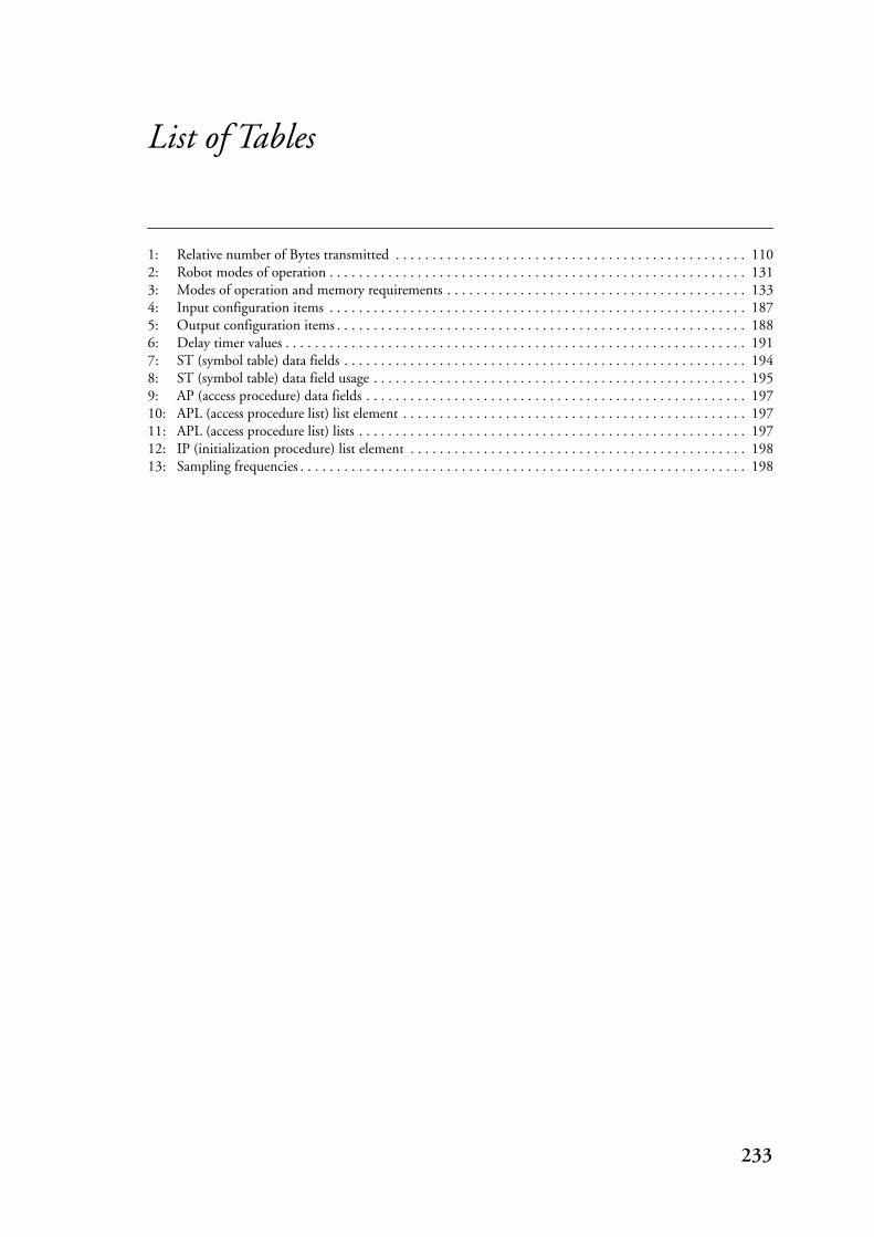
List of Tables

1: Relative number of Bytes transmitted . . . . . . . . . . . . . . . . . . . . . . . . . . . . . . . . . . . . . . . . . . . . . . . . 1102: Robot modes of operation . . . . . . . . . . . . . . . . . . . . . . . . . . . . . . . . . . . . . . . . . . . . . . . . . . . . . . . . . 1313: Modes of operation and memory requirements . . . . . . . . . . . . . . . . . . . . . . . . . . . . . . . . . . . . . . . . . 1334: Input configuration items . . . . . . . . . . . . . . . . . . . . . . . . . . . . . . . . . . . . . . . . . . . . . . . . . . . . . . . . . 1875: Output configuration items . . . . . . . . . . . . . . . . . . . . . . . . . . . . . . . . . . . . . . . . . . . . . . . . . . . . . . . . 1886: Delay timer values . . . . . . . . . . . . . . . . . . . . . . . . . . . . . . . . . . . . . . . . . . . . . . . . . . . . . . . . . . . . . . . 1917: ST (symbol table) data fields . . . . . . . . . . . . . . . . . . . . . . . . . . . . . . . . . . . . . . . . . . . . . . . . . . . . . . . 1948: ST (symbol table) data field usage . . . . . . . . . . . . . . . . . . . . . . . . . . . . . . . . . . . . . . . . . . . . . . . . . . . 1959: AP (access procedure) data fields . . . . . . . . . . . . . . . . . . . . . . . . . . . . . . . . . . . . . . . . . . . . . . . . . . . . 19710: APL (access procedure list) list element . . . . . . . . . . . . . . . . . . . . . . . . . . . . . . . . . . . . . . . . . . . . . . . 19711: APL (access procedure list) lists . . . . . . . . . . . . . . . . . . . . . . . . . . . . . . . . . . . . . . . . . . . . . . . . . . . . . 19712: IP (initialization procedure) list element . . . . . . . . . . . . . . . . . . . . . . . . . . . . . . . . . . . . . . . . . . . . . . 19813: Sampling frequencies . . . . . . . . . . . . . . . . . . . . . . . . . . . . . . . . . . . . . . . . . . . . . . . . . . . . . . . . . . . . . 198

233

List of Tables

234

Index

Aabstraction

deficient 10, 97in development 9, 37from implementation 66level of 11–12, 18–19, 35–36, 49–50, 58–59,

62, 79–80, 92–93, 95–96, 115, 171,174–175

acc. See generator, grammar, scanner, syntaxaccess

distribution 199–200input 100interleaved 100low-level 98module 194multiple 99multi-stage 100output 100, 113procedure 197

accuracyinterval 207measurement 207sensor 24signal 24temporal 218

action 55, 93CIP 94, 207irrevocable 213message 54–55, 57–59, 113phenomenon 53–56, 207

actuator 36, 219device 207

agreement, semantic 217alarm, shower 207aliasing, problem 21, 207API. See interfaceapplication

industrial 174software 207

architecture 32–34, 49–50, 207component 32–34, 50–51, 62, 66, 73, 80configuration 178description language 61, 66–68, 178implementation 33–34, 50–51, 62, 64–65operational 33–34, 50–51, 62style 66–68

ASIC 207assertion 207assumption

for analysis 45

assumption, cont.coverage 58, 208

ATM 208attachment, declaration 182availability

assessment 25of energy converter 142resource 24–25of sensor/actuator 52of a system 208system 28

BBackus-Naur Form 203–206, 208bandwidth

channel 208waste of 99

behavior 208abstraction of 96change 86continuous 81correct 15deterministic 12, 27, 118dynamic 121essential 92functional 49, 54, 159non-deterministic 44predictable 18, 29reactive 18, 30, 36, 53required 52–55

binary countdown. See bit dominance protocolblock, reactive 81, 90BNF. See Backus-Naur Formbottom-up 31–32, 66bounce, contact 209buffer 165–166bus

address 207data 210field- 27, 46, 212mezzanine 154VME 154, 160

busy waiting. See polling

CCAN. See networkcarrier

board 186production 186

235

Index

cascadeCIP 95execution 81motor controller 95

CDIF 7channel

access delay 208bit-length of a 208capacity 102CIP 83–84

characteristics, application 173CIP

machine 90method 78, 80, 208shell 90unit 68, 80, 90, 125, 132, 164–165, 181

CIP Tool 80class, frequency 106clock, device 208cluster

CIP 160, 208activation 85

CNI. See interfacecode

functional 91, 117structure 119as switch 117table 118

generated 88generation 35, 42, 99, 105, 177generator 174legacy 36, 41, 63, 79, 121object 35, 50, 59reentrant 216static 130

communication 49, 209asynchronous 26bandwidth 27broadcast 208buffer 98channel, motor controller 83CIP 83controller 209interface 114latency 27–28message 98, 114multicast 214net, motor controller 84network 214protocol 215semaphore 217synchronous 26traffic 28

compiler 209cross- 209

complexity 49, 62, 158component

architectural element 61

component, cont.connective 69declaration 180event extractor 69functional 68, 75, 80Hybrid III 141reuse 32, 175

composability 209composition 31–32, 41, 78concern, separation of 36concerns, separation of 6, 11, 36, 50, 158condition

CIP 89reasonableness 216

configurationconnection 158definition 129dynamic 129flexibility 47strategy 130

congestion, of a network 209connection 37, 159

chores 98configuration 209specification 98

connectorarchitectural element 61declaration 181high-level 71–72low-level 71

constantdeclaration 179production 185

construction 32of a system 209

contention 209context 209

switch 209control 36, 209

continuous 20algorithm 20

logical 213temporal 218

controller, programmable logic 8, 215conversion 120

A/D 99cooperation

asynchronous 78synchronous 78

CORBA 26, 209correctness

functional 16partial 214of program 34temporal 16

cost, per node 47CPU 209CRC 209

236

Index

CSMA. See protocolCSP. See formal methodCVT. See transmission

Ddata

acquisition 103conversion 98, 103dynamic 130encoding 210measured 213module 194output 98range 24raw 98, 216representation, internal 101structure

atomic 208dynamic 117

transport 104, 108verification 104width 99

deadline 22, 45, 210hard 20, 212interval 210soft 23, 217

deadlock 210debugger 17, 210declaration

attachment 182component 180computation 181connector 181constant 179glue 182instance 182message 181port 180role 181type 179version 179

decomposition 31–32, 49, 145delay 188

accumulation of 106channel access 208conversion 100propagation 215variation. See jitter

descriptionalgorithmic 76, 79appropriate 173behavioral 60, 76boxes with lines 50, 61–63formal 98informal 64non-formal 96

design, of a system 210

developmentconcept 6cross- 17, 30emphasis 7gap in the 30independent 51, 63, 157loop 8–9method

CIP. See CIPJSD 78, 213ROOM 78SDL 19, 78, 217Statecharts 19, 78, 217See also formal method

model 37phase 49problem-oriented 58, 66, 75, 171strands 156

deviceaccess 99, 102

time 100input 57with input and output 101peripheral 97, 100transducer 219virtual 97

dispatching, sequential 91display, production 192DMA 149, 210domain

classification 57controlled 52

download 210driver, device 210DSP 211duration 211

EEDF. See earliest deadline first schedulingemphasis

on functionality 8on implementation 7

encoding, of discrete values 102energy

consumption 135density 137efficiency 137recovery 139storage 137–138

engineinternal combustion 137

control 163environment 16–17, 39, 49

static 174of a system 211

equation, difference 210error 211

Byzantine 208

237

Index

error, cont.masking 211transient 219

ESTEREL. See formal methodEthernet. See networkevent 53–58, 93, 211

CIP 94, 211configuration 189discrete 19extraction 57, 98, 111–112, 120–121

algorithm 112hysteresis 111message 54–55, 57–59, 111phenomenon 211primary 215process 93production 192–193sporadic 19, 22temporal 93

evt. See generator, grammar, scanner, syntaxexception 211exclusion, mutual 214execution

path 118worst case See worst case

periodic 19–20, 117property 68, 72, 115, 173sequence 100, 116–117time 39, 106–107, 116, 122–125, 187–188

measurement 25, 106worst case See worst case

executive, run-time 123exhaust gas

cleaning 139, 142emissions 138

extensionof finite state machine 77–79, 82, 88, 90of formal model 79motor controller 90

Ffailure 17, 211

malign 213rate 29, 212timing 219value 219

fairness 212fault 29

device 29, 212hypothesis 212tolerance 18, 29–30, 212

application specific 207systematic 218

transient 219filter

anti-aliasing 21, 207low-pass 103, 124, 213setting 99

FIT. See failure rateflow control

back pressure 208explicit 211implicit 212transmission 212

flywheel 141FSM. See formal methodfunctionality 37, 159

Ggenerator

acc 159, 183, 194dsp 159evt 159, 189symbol table 194

glue, declaration 182grammar

acc 205evt 206pvt 203

Hhardware 212

capacity 43Hybrid III, broadcast 152peripheral 98–99resource 216topology 64

HI input. See input productionhierarchy 78, 145

motor controller 87host 212hybrid

concept 136parallel 137, 139serial 136vehicle 135

Hybrid IIIcluster IO 162, 166cluster O 165clusters 146clusters CEMHS 167component group 154configuration 158connection 159control system 145functionality 159modeling 158power supply 155processing node 157project

description 138structure 160

satellite 154signal conditioning 162simulation 157

238

Index

Hybrid III, cont.structure

implementation 147operational 145

taskabyss 165adaptor 165broadcast receiver 165, 169broadcast sender 166CIP 165, 170clock 166communicator 151, 165, 170event extractor 167input 152input converter 166monitor 165output 152output converter 166receiver 169sender 169strategy master 148submaster 148system master 148tick generator 165

working cluster 167

IICE. See internal combustion engineimplementation 41, 49

assembly 173assembly of 171constraint 42deterministic 81distributed 125efficiency 110lean 11–12simulation 126single-processor 125finding suitable 127variant 99, 124–125, 129

include, production 185industry 173initialization 186

init, production 186procedure 198

input 36, 49, 52–58, 99, 101access

interrupt 100static schedule 100as task 100

configuration 183data, distribution 108device 57production 187routing 154schedule 105–106, 120as task 122

inquiryCIP 83, 213motor controller 89

instance, declaration 182instant 213instantiation 213interaction

asynchronous 79, 83CIP 84, 213cyclic 85higher-order 78, 86–87internal 95net, motor controller 84pulse 85restriction 95synchronous 79, 84tree 96

motor controller 96Interbus-S. See networkinterface 213

abstract 97API 207CNI 208communication 83high-level 93instrumentation 97, 213interaction 83low-level 32MMI 214M-module 170node 213virtual 81, 93–94VME-bus 166

interrupthardware 100, 213latency 213procedure 41service routine 213

IO_Init, function 186

Jjitter

communication 27, 213input 20–22, 97, 106output 22processing 22, 29, 213

JSD. See development method

Kknowledge, a priori 17, 44, 46, 207

LLAN. See networklife sign 213link

broadcast 151failure 151, 154, 165

protocol 150

239

Index

LL. See least laxity schedulingload

distribution 105hypothesis 25, 213peak 25, 214processor 105, 107

loop, unbounded 117LOW input. See input production

Mmachine

CIP 90connection 58control 52finite state. See formal methodfunctional 57–58Mealy 76, 79, 212Moore 212reactive 91

maintainability 213management, thermal 141mask. See pattern productionmaster-slave

connector 87graph 87relationship 87

measurementaccuracy 101performance 40precision 215quantization 216representation 101rotor speed 162

mechanism, run-time 131MED input. See input productionmembership, service 214memory

allocation 117fragmentation 212

messageaction 54–55, 57–59attribute 93communication 214declaration 181delay 28, 46event 54–55, 57–59size 28

methoddevelopment

CIP. See CIPJSD 78, 213ROOM 78SDL 19, 78, 217Statecharts 19, 78, 217

formalCSP 149, 210ESTEREL 78, 211FSM 19, 76, 212

method, cont.formal

Petri Net 19, 215VDM 19, 219Z 19, 219

M-ICX. See internal combustion engine controlMMI. See interfacemode

change 86, 88CIP 86, 214of operation 174of operation. See operation modesetting 87

modelabstract 52behavioral, context 93checking 214CIP 91context 94essential 75formal 19, 75functional 50, 93–94, 158, 212

context 112context of 93

initialization 95life cycle 37states of a 54

modulegenerator 193M- 154, 161mezzanine 154, 186production 186

monitor, task 165motor, electric 137M-RPM. See rotor speed measurementMTTF 65, 214

NNBW. See protocolnetwork

backbone 27, 208CAN 46, 208collector 150, 164distributor 150, 164Ethernet 211FAST-bus 46instrumentation 27, 46Interbus-S 46, 213LAN 213Profibus 46, 215real-time communication 27, 216token bus 219token ring 219topology 46, 219WAN 27, 219

nodeinterface 213processing 16, 46, 64–65

240

Index

node, cont.production 191

Oobject, controlled 16observation

point of 215time-triggered 219

offset 214operation

atomic 208CIP 90, 214duty cycle 138–141initial 39mode 37–38, 157, 214

simulation 126order

causal 208temporal 70, 72, 75, 83, 218

orthogonality 36–37outptu, schedule 121output 36, 49, 52–58, 99, 101, 112, 121

access 113configuration 183production 188queue 113routing 154schedule 100, 113as task 122task 114

overload, protection 44

PPAR. See protocolparadigm, programming 36parallelism, conceptual 91, 118, 174parser, module 193pattern

abstract 96production 189

performanceanalysis 39–40, 42, 118average 17degradation 118increase 100measurement 118run-time 133system 18, 44verification 39worst case. See worst case

Petri Net. See formal methodphenomenon

controllable 52–53essential 55shared 53–55, 57of the world 52, 81

pivot 51, 66, 73PLC. See programmable logic controller

portdeclaration 180property 75

predictability 30, 41, 215preprocessor directive, include 185priority

dynamic 211fixed 45, 212inversion 44, 215message 47task 46

problemarea 12, 175connection 54–55, 57decomposition 49frame 52–57functional 54, 75separation 171

procedure call, remote 216process

activation, sequence 85, 95array 83behavior 39CIP 82, 159, 215controlled 209external 81, 94function 94interface 94master 213slave 217

processingrequirement, upper bound on 118time 118

processorgeneral-purpose 171load 99multi- 16, 71, 80, 214node 214single 16, 67, 115, 128, 164, 169, 189utilization 106–107

productioncarrier 186constant 185display 192event 192–193generator 179, 184, 190include 185init 186input 187module 186node 191output 188pattern 189slave 192timer 191version 185, 191

productivity 39Profibus. See network

241

Index

profile, automatic 117programming

language 34assembly 34–35, 173, 207C 34–35, 88, 106, 117, 208C++ 34–35syntax 8restricted use of 34–35, 42, 75

paradigm 34progress, independent 39property, deterministic 121protocol

bit dominance 208broadcast 151communication 215connection oriented 209contention 209controlled access 209CSMA 210efficiency 28, 46end-to-end 211flexibility 28latency 28, 46, 216media access 28, 46, 213NBW 214PAR 214point-to-point 151polling 215priority ceiling 215TDMA 218

pulseCIP 216multicast 85translation, motor controller 84transmission 85

pvt. See grammar, syntax

QQoS. See quality of servicequantization 20–21

Rrange

cruising 137of a value 24

real-timehard 212image, phase sensitive 72responsive 216soft 217

reconfigurationdynamic 128static approach 128–129

recursion 117region, forbidden 212relation

exclusion 101, 211precedence 215

relationship, behavioral 54reliability 18, 28–29, 65, 216relinquish 216repeatability 25report, CIP 96requirement

accuracy 24communication 26connection 55–56customer 17–19, 51, 53deduction 55functional 18, 53, 55implementation 25interface 59minimum 11real-time 23, 30reliability 28, 30temporal 19, 38–39, 44–45, 218timing 16

research, real-time system 173resolution 24resource

adequacy 24, 65, 216computational 209controller 216hardware 216management 17, 25, 43need 25software 216common use of 101utilization 12, 16–17, 40–41, 45, 174

response, predictable 121reuse

component 175software 175

risk, of testing 39RMA. See schedulingrobot

architecturecomponent 73implementation 64operational 63

communication, channel 91operation, mode of 131

robustnesscommunication 28, 46operational 47

role, declaration 181RPC. See remote procedure callRTOS. See operating system

Ssafety 216sampling 21, 217

decimation 210interpolation 213over- 22, 214polling 215

242

Index

sampling, cont.rate 20–21, 104, 106, 185, 198theorem 21, 217

satellite 154, 162scanner

acc 204evt 205module 193pvt 203

S-card 162schedule 217

global 122input 105, 120non-deterministic 44output 100, 113, 121processing 123–124run-time 118static 100

scheduler, module 193scheduling 217

cooperative 209cyclical 210dispatch 210dynamic 43–44, 122, 129, 211earliest deadline first 211laxity 213least laxity 213preemptive 44, 122, 211, 213, 215principles 43rate monotonic 45, 216round robin 45, 123, 216static 43, 122, 218time-sliced 45, 218

SDL. See development methodsection, critical 209selection, of signals 199semantics

acc 183–189CIP 80component 61composition 82evt 190–193formal representation 79–80programming language 42pvt 178–182

sensor 36, 217, 219intelligent 213

server, task 217service

quality of 27, 47remote 148

shell, CIP 90–91signal

conditioning 217continuous 101, 209conversion 114discrete 102, 210

encoding 102

signal, cont.pattern 111

simulation 38–39, 126–127, 157, 174implementation 99, 126

slavemotor controller 88plain slave 168production 192ring slave 168

solution, complete 173specification 174

connective 50language 75, 178, 183, 190

stability 217state 217

CIP 217continuous 94discrete 93ground 212inspection 85, 89instantaneous 79space, explosion 3, 76–77, 218transition 219

Statecharts. See development methodstructure

behavioral 86implementation 147operational 145

synchronizationexplicit 211implicit 213

syntaxacc 204evt 205pvt 203

systemCIP 218composition 31–32, 41control 15, 209decomposition 31–32, 145, 173distributed 16, 210drive 137embedded 15, 211event-triggered 18–19, 25, 211fail-operational 211fail-safe 211fail-silence 211hard real-time 16, 212heterogeneous 212hierarchy 145initialization 95operating 43, 214

RTOS 17, 216partitioning 91performance 44reactive 16real-time 16, 216safety-critical 28–30, 217

243

Index

system, cont.single-processor 16soft real-time 16, 23, 217sub- 218time-triggered 18–19, 25, 218

Ttable, off-line 130target 218

final 39task 218

active 207aperiodic 207blocking 208CIP 165control block 41, 218idle 212instance 218multi- 123, 214periodic 214preemption 44, 215priority 46, 215ready queue 216request time 218sporadic 44–45, 217suspension 218synchronization 41, 218

TDMA. See protocoltest

performance 39, 41schedulability 217stress 218on target 10

thrashing 27, 218tick 218

micro- 214time

execution 211to failure. See MTTFminimum between events 214rise 216

timeliness, guaranteed 25, 212timer, production 191timing, assertion 118token bus. See networktoken ring. See networktool 36–37, 159

domain 37integration 36

top-down 10, 31–32topology

bus 46hardware 33, 64, 219network 46, 219ring 46, 151

torque 138TRAM. See transputer moduletransaction, sporadic 47

transitionCIP 82, 84–85, 219structure 86

transmission, CVT 138, 141transputer 148–149

module 149, 160trigger 219TTO. See time-triggered observationtype, declaration 179

UUML 7, 96, 219unit, CIP 90–92unit. See CIP unituse, intermittent. See duty cycle operation

Vvariation, requirement 132VDM. See formal methodvehicle

hybrid 135interface 142

verification 39version

declaration 179production 185, 191

WWAN. See networkwatchdog 219WC… See worst caseweight 138worst case

administrative overhead 219behavior 28, 46communication delay 219execution

path 12, 39–40, 42, 91, 118–119time 124, 219

performance 17response time 47

Yyield 123, 219

ZZ. See formal methodzero-emission 139

244