Page 1
I
SLAC PUB 645 September 1969 (TH)
A THEORY OF DEEP INELASTIC LEPTON-NUCLEON SCATTERING AND
LEPTON PAIR ANNIHILATION PROCESSES. * II
DEEP INELASTIC ELECTRON SCATTERING
Sidney D. Drell, Donald J. Levy, Tung-Mow Yan
Stanford Linear Accelerator Center
Stanford University, Stanford, California 94305
Abstract:
This is the second in a series of four papers devoted to a theoretical
study based on canonical quantum field theory of the deep inelastic lepton processes.
In the present paper we present the detailed calculations leading to the limiting
behavior - or the “parton model” - for deep inelastic electron scattering. It
follows from this work that the structure functions depend only on the ratio of n
energy to momentum transfer 2Mv /q’ as conjectured by Bjorken on general grounds.
To accomplish this derivation it is necessary to introduce a transverse momentum
cutoff so that there exists an asymptotic region in which 4’ and Mv can be made
larger than the transverse momenta of all the virtual constituents or “partons”
of the proton that are involved. We also derive the ladder approximation for the
leading contribution, order by order in the strong interaction and to all orders in
the coupling, to the asymptotic behavior of these structure functions with increasing
ratio of energy to momentum transfer, Finally we draw and discuss the experimental
implications.
*Work supported by the U. S. Atomic Energy Commission
(Submitted to Physical Review)
Page 2
I. INTRODUCTION
This is the second in a series of four papers devoted to a theoretical study
based on canonical quantum field theory of the deep inelastic lepton processes
including (along with other hadron charges and SU3 quantum numbers)
e +p--+e “anything” + e +e-+p+ 11
LJ+p-+e+ I?
-G-p + --+e+ rf
Electron scattering from hadron targets, and the crossed channel process of electron-
positron annihilation to hadrons, share a singularly attractive feature relative to
the various processes of hadrons scattering from hadron targets: the electro-
magnetic field generated during the electron’s scattering is understood if indeed
anything is in particle physics. Dirac tells us the transition current of the scat-
tered electron and Maxwell tells us the rest. Therefore in these processes we are
probing the structure of the hadron by an electromagnetic interaction of known form.
There is an additional advantage in studying this process and that is its weakness.
We can do our theoretical analyses to lowest order in the fine structure constant
o z -&$, which is a comfortable expansion parameter for quantitative results.
Similarly to the extent we have confidence in the V-A theory of weak couplings
the neutrino reactions directly measure the matrix elements of the hadronic weak
currents and can in principle and in practice be related to the electron processes.
Certain structure functions of the hadron summarize these processes when
we detect the energy and momentum of only the one particle indicated explicitly
in the above list of reactions and sum over all other final states. This summation
over all other hadron states permits us to make headway with the theoretical
-2-
Page 3
formalism by making full use of unitarity and completeness. As a result, the
distribution of the secondary particles will not be analyzed in detail in our approach.
Nevertheless, statements about certain characteristic features of the secondary
particle distribution still can be made.
In Paper I, 132 we placed primary emphasis on the physical ideas behind the
proofs showing how the structure functions of the electron-nucleon scattering in the
Bjorken limit of large momentum and energy transfer become universal functions3
of the ratio of momentum to energy transfer and probe the longitudinal momentum
distribution of the “elementary constituents ‘1 in the nucleon in an infinite momentum
frame; how the continuation of these structure functions below the inelastic scat-
tering threshold give predictions for “deep inelastic I1 electron-positron annihilation
into a p’roton plus everything else; how the neutrino and anti-neutrino scattering
are related to each other and are closely connected with inelastic electron scattering.;’
and finally how one can understand, at least qualitatively, both the rapid fall-off of
the electromagnetic nucleon form factors for elastic scattering with increasing
momentum transfers and the nonvanishing structure functions for deep inelastic
electron-proton scattering. In this second paper of the series we present the de-
tailed calculations leading to the limiting behavior - or the “parton modell’ - for
deep inelastic electron scattering. We also derive the ladder approximation as
discussed in Ref. 1 for the leading contribution, order by order in the strong inter-
action and to all orders in the coupling, to the asymptotic behavior of these
structure functions with increasing ratio of energy to momentum transfer. Finally
we draw and discuss the experimental implications. 5
The interpretation of our formalism depends heavily on the use of the old-
fashioned perturbation theory in an infinite momentum frame. Therefore,
section II is devoted to a brief introduction to rules for calculations in an infinite
-3-
Page 4
momentum frame. Some peculiar phenomena occurring in such a reference
frame are discussed. Calculational developments appear in Sections III and
IV and the Appendix, and experimental implications are presented in Section V.
The analogy between the Bjorken limit and nuclear physics sum rules is also
discussed.
II. PROPERTIES OF AN INFINITE MOMENTUM FRAME AND
OLD-FASHIONED PERTURBATION THEORY
As first shown by Bjorken3 the infinite momentum frame of the proton is
very useful for studying the structure functions of the proton (hadrons) in the
limit of large momentum transfer Q2 and large energy transfer My , with the
ratio w = 2Mv/Q2 fixed. Reasons for looking in this asymptotic kinematic region
in search of both a simple, general behavior and interpretation of the structure
4,6 functions have been discussed elsewhere. Feymnan in particular has emphasized
that in a high energy limit so that the incident electron and proton are both very
relativistic in their center-of-mass frame, the proton may be viewed as an as-
semblage of “long-lived” or almost ?free” constituents as a result of the time
dilation. If the energy transfer from the electron to the proton is also large as
viewed in this same frame the interaction may be treated as a sudden pulse.
During the brief duration of this pulse the constituents - or “partons” - of the
proton can be treated as instantaneously free so that an impulse approximation
will be valid. The kinematic conditions for this to be a valid approximation are
-4-
Page 5
P-GO and P>>2Mv,Q2 2 BMV--cc, Q-00 with
(1)
(2)
w = 2Mv/Q2 finite and Q2(w - l)-+ tc .
This is the Bjorken limit in which we shall work. Since the validity of the
picture of long-lived constituents of the proton that are almost “free1Y is important
to help our intuition we shall find it useful to work in an infinite momentum frame
in formulating our theory in detail. This section develops the simplifications as
well as delicacies of doing field theory in such a frame.
The modern perturbation theory developed by Feynman, Schwinger and Dyson
makes explicit the relativistic covariance of the S-matrix at the expense of mani-
fest unitarity by grouping together intermediate states with different numbers of
particles and antiparticles. On the other hand, in the so-called old-fashioned
perturbation theory unitarity is more visible but manifest relativistic covariance
is lost. Weinberg’ pointed out that by applying the old-fashioned perturbation
theory in a reference frame of infinite total momentum there are substantial
calculational simplifications, and a new set of rules appear with properties in-
termediate between those of Feynman diagrams and those of old-fashioned
diagrams. Weinberg found in +3 theory that the energy denominators become
covariant and all intermediate particles must move forward with respect to the
total infinite momentum. This latter property prevents creation of particles
from the vacuum and greatly simplifies both the interpretation and calculation
of the theory.
Unfortunately, as pointed out by Chang and IV& 8 working in an infinite
momentum frame requires extreme care. They showed, for example, that in
$3 theory vacuum diagrams (diagrams with no external lines) which should
vanish according to Weinberg’s rule acquire nonvanishing contributions from
-5-
Page 6
end points of allowed longitudinal momenta carried by the internal particles.
More complications arise in a theory of particles with spin, as we shall illustrate
below. However, we should emphasize that despite these unpleasant complica-
tions it still can be useful to work in an infinite momentum frame. This is true
if we are dealing with amplitudes in which intermediate states are long-lived because
of relativistic time dilation, If this is the case, the internal particles are almost
real and the violation of energy conservation can be ignored. It is precisely this
property which enables us to derive the parton model as sketched in Paper I. It is a
property of particular amplitudes and of special kinematic regions and not of the
theory in general, however. Therefore, it is not a general simplification for all
processes as will become clear in the following.
In the model discussed in Paper I, i. e. , the canonical quantum field theory
of pseudoscalar pions and nucleons with charge-symmetric Y5 coupling, the
strong dynamics of the pion-nucleon system is described by the interaction 3
Hamiltonian
HI(t) = ig J d3x6& t) Y~~v!‘C~, t) - 1 (x,, t)
where it is understood that mass renormalization counter terms for the nucleons
and the pions are implicitly included. The electromagnetic current of the hadrons
is
Equations (1) and (2) do not give a full statement of the theory in our model
for the following reason. The value of working in an infinite momentum frame
lies in the simplification of being able to label intermediate particles in a pertur-
bation calculation according to whether they are moving along or in the opposite
-6-
Page 7
direction to the infinitely large longitudinal momentum defining the reference
frame. Such left-right distinctions are only clear and useful if the transverse
momenta at all interaction vertices are small in ratio to the longitudinal
momentum. In our theory this requires us to introduce a transverse momentum
cut-off in doing the calculations. This point was discussed more fully in I and
its need and role will become clearer in the following formal developments.
As discussed in I it will be useful to undress the Heisenberg operators ,and
go into the interaction picture by the usual U-matrix transformation. For ex-
ample, the Heisenberg current operator JP(x) and the corresponding bare or
free current j,(x) are related by
J&x) = U-l(t) j,(x) U(t) (3) where
U(t)= exp -i ( [ g,;HI4) + (4)
and jP has the same form as (2) written in terms of the free particle in-fields.
A basic formula in the old-fashioned perturbation theory which we repeatedly
employ is
+ C ’ In2><n2 IHI 1 rip-y f+(O) 1 a>
“ ’ (“’ nln2
(Ea-En -&)(Ea-En -ie) 2 1
u = U(0) where C’ indicates the summation over all intermediate states except the
initial state a; and Za, the so-called wave function renormalization constant,
is determined by the normalization condition
<a’ IU-%Jla>= daa, .
The states in (nl>, ]n2>, etc., are properly symmetrized (antisymmetrized)
with respect to identical Bosons (Fermions) present in these states.
. -7-
Page 8
The value of undressing the current in (3) and of assembling the strong
interaction effects into the description of the states lies in the possibility of
classifying terms in the infinite momentum frame. One can separately study
the behaviors of the energy denominators in the expansion (5) and of the bare
vertices introduced by the interaction matrix elements in the numerators of (5)
as well as by j,(x) and identify the leading terms in an infinite momentum limit.
We turn first to the properties of the vertices. To study the properties of the
bare vertices in an infinite momentum frame it is convenient to use the familiar
representation of the Dirac matrices: 9
whereg= (ol, ~2, 3 cr ) are the 2 x 2 Pauli spin matrices. The positive (negative)
energy solutions of the Dirac equation, denoted by U+ (v,) are
111 --
(8)
where + and - denote the solutions with the third component of the spin in the
rest system pointing up and down, respectively; and U&are two-component Pauli
spinor s.
-8-
Page 9
In terms of these spinors the bare y, vertex has the following properties,
as the momentumg tends to infinity along the third axis:
772 -- k q1 -11 )-a3M(1
w= ‘71,p+$J Y5”F 772- -21 P+k ) = - 2v4xP UT U2
where 5, q2 are positive numbers and$ll,c21 k are the transverse momenta.
Specifically by infinite momentum limit we mean that the ratio kL /P - 0 for all
k I . As mentioned earlier to enforce this condition it is necessary to impose a
cutoff on the theory described by (1) and (2). The important thing to notice in
(9) is that when both nucleons (anti-nucleons or nucleon and anti-nucleon) move
opposite to each other the vertex becomes infinitely large as P; when they both
move forward the vertex is of order unity. It is this peculiar property that in-
validates Weinberg’s original argument that all particles must move forward
along the direction of the infinite total momentum.
-9-
Page 10
I
We also need the properties of the bare electromagnetic vertex of the
nucleon current in the infinite momentum frame. They are
(10)
where,& (2) denotes y1 or y2 (OYY or 02). The matrix elements v1 yp v2 can be
obtained from above by charge conjugation. They are very similar to the cor-
responding ones 4 yp”2 l
The important thing to notice in (IO) is that for the
time component and the third component of the nucleon current the electro-
magnetic vertex does not have the abnormal property exhibited by the pion-
nucleon vertex; namely, the electromagnetic vertex does not introduce any extra
power of P when the two nucleons (two antinucleons or nucleon and antinucleon
pair) at the vertex have opposite longitudinal momenta, This is also true for the
electromagnetic vertices of the pion current. For the transverse components
of the nucleon current the electromagnetic vertex behaves exactly the opposite.
Therefore, if it is possible to restrict our attention to the time and third component
- 10 -
Page 11
I
of the electromagnetic current, then Weinberg’s argument holds and no particle
of negative longitudinal momentum may enter or leave the electromagnetic vertex.
For this reason the time component and the third component of Jcl are referred to
as “good currents. l1 10 For processes such as the electron-proton scattering in
which the bare current acts only once in the one photon exchange approximation
it is possible to use only the good currents, and take full advantage of Weinberg’s7
arguments; the contributions from the transverse components can be inferred
from covariance requirement.
To illustrate the techniques of calculation in an infinite momentum frame
and simultaneously develop several useful results for the calculation of nucleon
structure in the next section we compute to second order in the coupling (1) the
wave function renormalization constants Z2 and Z3 for the nucleon and the pion,
the mass renormalizations dM and dp2 for the nucleon and the pion, and the
electromagnetic vertex renormalization constant Z1. The wave function re-
normalization constant Z2 for the proton is defined by
<P y5”P 1 Ep- E14.$ I Plkl ’
where 1 P > is a one-proton state with momentum 2 and energy El; and 1 Plkl >
is a state with a proton of momentum I& and energy El and a neutral pion of
-ll-
Page 12
momentum & and energy ol, etc. The contribution of charged pion can be cal-
culated similarly. We have defined
u = U(0)
The normalization condition
< UP 1 UP’ ’ = d3 (g-g:‘,
determines Z2. To order g2 we have
(12)
(13)
(-2) (M2- PP,) 2
(Ep-yq
This is represented graphically by Fig. la where as always the solid lines
are for nucleons and dashed ones for pions. The contributions from Fig. lb
and lc will be discussed shortly - as will their absence from (14). Let us
parametrize the momenta as follows
I?,=~~+&, , kl= (l-J7)P-$, , lag .g= 0 .
In an infinite momentum frame, p--+00, we have
(15)
Ep-YJl= b+g] -~vlP+gq- [p-q,+ $+;yp ]
=2VP+O $ ( )
, rl<o
ZZ 2(&1)P + 0 (+) > 77 > 1
ky + M2(1-r))2+ p2rj =-
27?(1-7l)P , O<rl<l
- 12 -
Page 13
and
-2(M2- .P .Pl) = 477P2 + O(1) , 77< 0
1 ,V>O. (17)
Notice that if all the particles move forward, i.e. , both V and (1-q) are
positive, the energy denominator E P
- El - G),. is proportional to -$ ; on the
other hand, it is proportional to P if any of the particles in an intermediate state
moves backward, i.e., either ?j’ or (1-q) is negative. When there is no possibility
of ii:::,zlucing compensating powers of P in the numerator as in G3 theory, :his
property enables Weinberg to conclude that all particles must move forward.
But from (9) or (17) we see that in a theory of particles with spin such as (1)
when one of the nucleons moves backward, the vertex becomes proportional to
P. The change of P2 in one energy denominator can be compensated by two big
vertices. An example of this kind is provided by the calculation of bM below.
In the case of Z2 as given by (14) a simple inspection shows that only when
the rl defined in (15) is between 0 and 1 is the integral nonvanishing as P- =.
It is this property which makes the infinite momentum frame so useful;
namely, the q integrations are restricted to certain well-defined intervals.
where the subscript 7r” indicates the contribution of neutral pion to Z2. The kf
integration is logarithmically divergent, as expected from covariant perturbation
- 13 -
Page 14
theory. The corresponding charged pion contribution to Z2 can now be written
down. It is
In the above discussion we have temporarily ignored the contributions of
four - particle intermediate states to Z2 represented by Fig. lb and Fig. lc.
According to the old-fashioned perturbation theory, as in the covariant perturba-
tion theory, we are instructed to omit all disconnected diagrams in calculating .
a physical amplitude. Thus the contribution of Fig. lc should be excluded. The
contribution of Fig. lb is given by an expression similar to (14). Its value is
zero as P-m, since at least one of the intermediate particles has negative
longitudinal momentum. The two large vertices in the numerator are not
enough to overcome the large energy denominator squared in (14).
The wave function renormalization constant for the pion, Z3, can be
computed analogously. The result is
4(M2-P. F)
2j7(w-E-F) 2 1
dq k;+M2
(20)
The diagrams contributing to Z3 are shown in Fig. 2.
We now compute the contribution to Z1 from one ?r” exchange. The contri-
bution from charged pion exchange will be included later. In general there are
six time-ordered diagrams as shown in Fig. 3 contributing to the vertex
- 14 -
Page 15
I
corrections. Equation (3) gives
<PIJcL(0)(P’> = <UP~jp(0)lUP*> (21)
To compute Z1 set q = P1 - P = 0. Using (9), (10) and (21) one concludes that
for good currents only diagram (a) in Fig. 3 contributes.
The situation is different for transverse components of the current to which
other diagrams also contribute. For example, in diagram (b) and (.e) if we write
(22) kI = (1-t))P- k,
then the region 0 < ?? < 1, where the antiproton moves backward, contributes.
Although one of the energy denominators in this region is of order P, instead of 1 ( Fy it is compensated by the powers of P introduced at the large strong vertex
and at the large bare electromagnetic vertex of a transverse component. However,
if both the proton and antiproton move backward, then both the energy denominators
are of order P and are too big to be compensated by powers of P introduced at the
vertices. As a result allowed values of Q are restricted to O< 9 < 1.
Diagrams (c), (d) and (f) never contribute since both energy denominators in
these diagrams are of order P. This is a general rule. By simple power counting
two big vertices are always required to compensate one big energy denominator.
Therefore, a particle created with negative longitudinal momentum must either
be absorbed or change its sign of longitudinal momentum at the next vertex. It
cannot traverse beyond a vertex without being disturbed. This result eliminates
many otherwise possible diagrams in an infinite momentum frame and it will be
repeatedly utilized without explicit reference in our subsequent discussion.
- 15 -
Page 16
Relativistic covariance of the theory allows us to compute Z1 by restricting
Jcl to good components (p = 0 or 3) ; then only Fig. la contributes. Obviously,
one can compute Z1 using the transverse components of J . But then extreme P
care and extra labor are needed. From the definition of Z1 and using good cur-
rents we have
Ii Y u (Z -l-q = u PclP 1
-Jwi (Z -l-l) PM ~1
ip(M-~Pl)y AM- YP1)up 2
Gq (Ep-EpJ$ 2
d-1 - J
d3kl (-2)(M2-PPl)ii Pl u 2 (271)~ M 2‘+ (2El) (Ep-El-ul)2
(23)
Using the parametrization (15) and P lcl = QPcl for /A = 0, or 3, we obtain to order g2,
Zl(#) = 1-L
167r2
1 2
JJ % 2 drl (l-59 k;+M2(1-v) 2 2 2 0 k,2+M2(l-q) +/A q I
In comparison with (18) we find
Zl(?ro) = z2(nq
provided the cutoffs for the k: integration in both expressions are identical.
This identity of renormalization constants is required by the Ward identity.
Contributions to Zl due to exchange of a charged pion also include six
diagrams in general as shown in Fig. 4.
(25)
- 16 -
Page 17
A simple power counting shows that only Fig. 4a contributes for any of the
four components of J . Calculations similar CL
to (23) give
P u -P u (z;l-1) = -$
PM P t-2) W2- PP,)
!h Gq tEp-“l-y) 2
ii P WIUP (26)
The parametrization (15) gives for p = 0 or 3, to order g2 , 1
drltl-7)) k;+M2(1-1) 2
kf+M2(1-q) 2 2 2 (27) -I-P rj
0 I
which shows, again in accord with the Ward identity,
z1(7?) = z2( ??+) . (28)
If one chooses ,u = 1,2, then (26) is a trivial identity. The left-hand side of
(26) vanishes because Pin has no transverse component and the right-hand side
vanishes after symmetrical integration of k .
The second order mass renormalization of a nucleon, dM, can be computed
by the familiar formula for second order energy-level shift in the old-fashioned
perturbation theory
dEn=C E E (29) m n- m
where the summation C 1 excludes m = n. Equation (29) and the mass shell re-
lation Ei = P2 + M2 give
bM- 2 pp,lH~~~/n~12 .
n P n (30)
The charged pion contribution will be ignored since it can be obtained trivially
from the neutral pion contribution.
- 17 -
Page 18
I
We reproduce this calculation to illustrate an example in which extra care
must be taken in dealing with the extremes of the dq integrations. To order
g2, there are three contributions corresponding to the three diagrams in Fig. 1.
Again the disconnected diagram Fig. lc will be omitted. The contributions of
Fig. la and lb, denoted by bMa and 6M,, respectively, are
d3k, -(M2-PP1) - 29 2E,(Ep-E1-~l)
a,,=L 1 d3kl (M2+ PFl)
(~3~ M J -
F 2~l(Ep+E1+~l)
where the momentum labels are indicated in Fig. 1. For 6M, using the parametri-
zation (15) and taking the limit P -+ 00 we find that there are two regions of q con-
tributing, 0 < q < 1 andq< 0, corresponding to the intermediate nucleon moving
forward and backward. Thus
dM a
= &qtl) + aM(2) (3) a a +6Ma (32)
&/I@) = ds m!L a 167r2 2M
1 k;+M2( 1-r)) 2
k;+M’(l-q) 2p2q (33)
&t2) = 2 1 a 16,” 2M
(34)
Since the resulting 77 integrations diverge at tl= 0, a small cut-off g is given to
both sides of rl = 0. The contribution from the infinitesimal region - c <Q< e is
denoted by 6MF) . For 6Mb the following parametrization for the momenta is used
(35)
- 18 -
Page 19
I
In the limit P+ CC we find
dMb = dMf) + dM@) + dMt3) b b
drl 167r2 2M 1-v
d&f) = 82 -!L 167r2 2M
1-r
(36)
(37)
(38)
Again the resulting r] integrations diverge at tl= 1. For simplicity and anti-
cipating the procedure to be correct, the same cut-off E as in 6Ma is given to
both sides of q= 1 here. The contribution from the infinitesimal region
1 -e < rl <l +e is denotedby dMf). Collecting we obtain
+ de) + dMP (3g)
Since the q integration in the first term converges now, the cut-off E is un-
necessary and therefore is set to zero. It is interesting to notice that if 6Mr)
and dMAq are ignored, dM vanishes with p2, in conflict with the known result in
covariant perturbation theory. Thus, the main contribution to dM must come from
the infinitesimal regions of 77, i.e., 6M(3) and aMf) . a We verify this statement
by explicit calculation. Using (15) we have for Q- 0
-(M2 - PP1)= -P[?lP-j@ZG?]
E P
-El-Li=:‘IP- q2P2+kf+M2 J
- 19 -
Page 20
and
i.e.,
d&&q = de 1 a 167~~ 2M /
Similarly using (35) we obtain
(42)
(43)
Observe that aMr) and aMf) separately diverge as P-CO or e-0.. The sum of
the two, however, becomes independent of both P and E .
,jMt3) + dMt3) = 82 1 a b 167r2 2M /
&f h k’+M2 k;+p2
(44)
Finally, dM can be written in the parametric form
M(l-r)) k,2+M2(1-7) 2+p2
(45)
which can be verified to be in agreement with covariant perturbation calculation.
The mass renormalization of a pion, &..A~, can be computed similarly. We
record here only the contribution of the diagram of Fig. 2b in which both inter-
mediate particles move forward. This contribution will be referred to later.
It is
j $‘1 Tr {WYPll Wyiil)) .
1 2~l(~,-E,-~l) w-3
- 20 -
Page 21
In this section we have seen in simple examples some of the subtleties in
the infinite momentum frame calculations. Sufficient care must be exercised if
calculations are performed in such a reference frame. As a general rule, there
is need to use extra care in handling a diagram if, and only if, after taking the
limit P- 03 and before doing any integration, the diagram diverges at the end
points of the rl integrations.
III. DERIVATION OF PARTON MODEL FOR DEEP
INELASTIC ELECTRON SCATTERING
We turn now to the physical process of inelastic electron-nucleon scattering.
We are interested in the two structure functions summarizing hadron dynamics
as probed by experiments that detect only the four-momentum of the outgoing
electron and sum over all hadron final states compatible with the overall con-
servation laws. These functions are labelled WI and W2 and defined as earlier
by’1
E w =-4X2 -$ PV /
(dx) e+iqx -1 J,C~J,P) I P>
<PIJI((0)ln><n J,(O)~P>(~Z)~~~ (q+ P - pn, (47)
XV ( i
= W1(q2, v) + gpv - q2 -$- (PC,- --y 4J Pv - = qv)W2(s2, v) q2
where I P > is a one-nucleon state with four-momentum P q is the four-momentum I-1’ P
of the virtual photon, q2 = - Q2< 0 is the mass squared of the virtual photon, and
Mu = q. P is the energy transfer to the nucleon in the laboratory system; W=2Mv/Q2.
An average over the nucleon spin is understood in the definition of W PV l
Since
- 21 -
Page 22
(q+P)21M2, we must have ,l < w < cg. If w = 1, only the elastic process
e f P-e’ + P1 contributes to (47). However, as long as w - 1 # 0 the invariant
mass of the final hadrons, (q + P)2 = Q2(w - 1) + M2, becomes very large as
Q2, MU-~ with w fixed. Therefore all possible inelastic channels contribute
to (47) in this deep inelastic region. Since we are interested in the deep inelastic
continuum and not the resonance excitations we shall always require
2Mv - Q2 = Q2(w-1) >> M2 in the following.
We perform our calculations in the infinite momentum center-of-mass frame
of the electron and nucleon P-COO, where P is the energy of the incident electron
and proton, and the components of the momentum transfer are
q”=*, q3= -2Mv -Q2 4P , I%] =@+o(-$) (48)
with the nucleon momentum2 along the 3 axis. We now undress the current
operator with the aid of (3) and rewrite (47) as follows
W clv = 4~~ &EUPl jcl(0)U/ n ><n IV-l jv (0) I Up*277)4d4(q+ P - Pn)
(49) In approaching the task of evaluating (49) we recall several general features
of old-fashioned perturbation theory that simplify our task. First the spatial
momentum is conserved at each vertex and the energy is not. This is already
clear in (11) where the momentum d-functions result from the volume integral
in the interaction (1) whereas the energy denominators arise from the time integral
from T = -,03 to T = 0 in the U matrix in constructing (5). Since the currents and
fields have been undressed by the U transformation,free bare particles are being
created and destroyed at the vertices and although not on their energy shells they
- 22 -
Page 23
are on their mass shells - i.e., of= kf + p2 and E 2 pi
= Pf + M2 everywhere.
Furthermore we understand that all disconnected diagrams are excluded 12 in
our discussions and calculations and in particular in the expansion of (49).
Many diagrams in the expansion of (49) vanish in an infinite momentum
frame which otherwise contribute. First we recall the general rule derived in
section II that a large or bad energy denominator requires two large vertices to
overcome it. This rule eliminates diagrams of the type shown in Fig. 5 if they
appear in the expansion of 1 UP > or U In > . In these diagrams either a pion
created from the vacuum carries a negative longitudinal momentum or a nucleon
(anti-nucleon) with negative longitudinal momentum traverses across a vertex
without being annihilated or converted into a particle with positive longitudinal
m.omentum.
We may also restrict our attention to good components of the current
jp, in (49)) i. e. , p = 0 or 3, since the covariant structure (47) allows us to infer
Wl and W2 from Woo and W33. In the infinite momentum frame where q is
almost transverse, as indicated in (48), the electromagnetic current does not
alter significantly (- +j relative to P) the conservation of longitudinal momentum
of the hadrons at the electroma.gnetic vertex. Then the discussion in the pre-
ceding paragraph shows also that an electromagnetic vertex cannot occur in between
two strong vertices where the intermediate state contains particles with negative
longitudinal momentum. Also a charged particle and its anti-particle cannot
annihilate at the electromagnetic vertex since they must have longitudinal momenta
opposite to each other. For these diagrams the powers of P introduced by the
large energy denominators are more than can be overcome by the large vertices
in the numerator. Therefore, diagrams as illustrated in Fig. 6 where the electro-
magnetic current operates at the vertex marked x are also eliminated in the
infinite momentum frame we are working in.
- 23 -
Page 24
We can also infer from these discussions the important conclusions that
all the final particles in the expansion of I UP > , i. e. , all particles existing at
the instant of the current interaction as given by (11)) and the real particles
present in the final states 1 n > must have positive longitudinal momenta. Suppose
there is one particle in IUP > moving with negative longitudinal momentum. This
particle may scatter or be annihilated by the electromagnetic current or may not
even interact with it at all. The electromagnetic vertex will not change the direction
of the longitudinal momentum of this particular particle if it does not interact with
the current or if it scatters from the current since the virtual photon has to order
$ only transverse momentum. As a result in these cases such a particle appears
in U]n > if it is present in IUP > and this thereby introduces at least two large
energy denominators and at most two big vertices. Since the two denominators
reduce the contribution by (P2)2 and two big vertices enhance it by at most P2 this
cannot contribute to leading order, The case in which this particle with negative
longitudinal momentum is annihilated, together with its anti-particle with positive
momentum, by the current is ruled out to leading order as discussed in the preceding
paragraph. Finally suppose there is a particle in the final state 1 n> moving with
negative longitudinal momentum. However this possibility is ruled out by the
energy conserving delta function in (49) since to leading order as P+ CO , we
must have that En -+ E z P. 13 P
In the Bjor.ken limit of large Q2 and Mu, (49) greatly simplifies. This simpli-
fication is intimately related to our fundamental assumption made in Paper I that
there exists an asymptotic region in which Q2 can be made greater than the
- 24 -
Page 25
transverse momenta of all the particles involved, i. e. , of the pions and nucleons
that are the (virtual) constituents or “parton& of the nucleon. Such an assumption
is consistent with present high energy data that strongly indicate that transverse
momenta of the final particles are indeed very limited in magnitude. In our
analysis we suppress large transverse momentum transfers by simply insert-
ing a transverse momentum cut-off at every strong vertex as commented earlier.
The cut-off procedure employed in our formalism is illustrated by the
following examples of typical diagrams in Fig. 7 contributing to (49). Along
with these examples we also illustrate how the allowed values of the longitudinal
momenta are determined. Consider the time-ordered diagrams in Fig. 7. The
vertical dashed lines intersect the real physical final states produced from the
initial proton by the current ‘which interacts at a vertex marked x. The momenta
for the nucleons and pions are indicated. For Fig. 7(a) and 7(g) the momenta
will be parametrized as follows:
For Fig. 7(b) they are parametrized as follows:
For Fig. 7(c) the parametrizations are
(59)
(51)
- 25 -
Page 26
For Fig. 7(d) and 7(h) we adopt the parametrizations
(53) 5 = “&$ +&2pr2 F = (l-n2)k&lC2L;o < n2< l*lC21’El = 0
The allowed regions for the 77 ‘s given above are determined by our observation
that all the final particles in IUP > and particles present in the final states I n >
must have positive longitudinal momenta.
Our cut-off procedure states simply that the squared length of the transverse
momenta kilts of each vertex as defined above never exceed a maximum value
kHmax* Notice that the “transverse momental’ ki ‘s are not defined with respect
to the fixed direction given by P. This definition of kills and the cut-off procedure
just described are reasonable since the cut-off, a property of a vertex, should
depend only on the characteristics at the given vertex and should be independent
of what has happened preceding it, The simple sharp cut-off procedure may be
replaced by a more elaborate smooth one such as a form factor. Such a procedure,
however, will not change the basic features of the general formalism but only de-
tailed numerical predictions of our model. Since our detailed predictions of this
kind as will be shown in the next section are insensitive to the precise cut-off,
we are justified to adopt such a simple cut-off procedure. In the present context
the entire and sole use of the cut-off is to make all integrals over intermediate
particle momenta finite as we let Q2 -.w so that we can classify leading terms in
a hierarchy simply according to numbers of powers of Q2 in the numerator minus
the number in the denominator.
Return to the other diagrams in Fig. 7. Suppose for Fig. 7(e) l?,,l~~, l?2 and
b2 are parametrized as (50) and El, &!!, &, l& are t o e e ermined by momentum b d t
- 26 -
Page 27
conservation. Because of the sharp finite cut-off for$il andiil , the relations
between primed and unprimed quantities are very complicated. Again we are
not interested in the precise numerical values but only in a classification ac-
cording to leading powers of Q2. For simplicity in these diagrams with
crossed lines we will use a slightly different parametrization. For instance
the momenta in Fig. 7(e) will be parametrized as follows:
where the allowed regions for nl and ni are such that all the final real particles
have positive longitudinal momenta. The parametrization (54) implicitly assumes
the complete overlap betweengp k2 and&i, 82 , although this is not strictly true
as the cut-off for the transverse momenta is finite. This particular parametriza-
tion has the advantage that it is symmetrical with respect to the two halves of the
diagram. In the same spirit we parametrize the momenta in Fig. 7(f) as given
by (54)) but the allowed regions for nl are different. Sincek: is the momentum
of a final real particle, l-‘7’1 can vary between 0 and 1. The nucleon with
momentum P2 is virtual and therefore may have positive or negative longitudinal
momentum, corresponding respectively to the two allowed regions of
ql: l’~l>(lVi), and (lTi)>~l>O.
We now turn to the simplifications introduced in our model of (1) with a
maximum transverse momentum cut-off when we go to the Bjorken limit. In
this limit certain classes of diagrams in (49) vanish. To make this simplifica-
tion apparent we consider the time-ordered sequence of events in the old-fashioned
perturbation theory description of a scattering process as represented by the matrix
- 27 -
Page 28
element <UP 1 jcc(0) U In> . Before the bare current jp(0) operates, 1 UP > describes
emission and reabsorption of pions and nucleon-antinucleon pairs. The bare
electromagnetic current scatters one of the charged constituents in 1 UP > and
imparts to it a very large transverse momentum 3 1 z J Q2 . The unscattered
constituents in 1 UP > keep moving and emit and reabsorb pions and nucleon-
antinucleon pairs. They form a group of particles moving very close to each
other along the direction P as large transverse momenta are suppressed by the
cut-off vertices. The scattered charged constituent also emits and reabsorbs
pions and nucleon-antinucleon pairs. Analogously these form a second group of
particles moving close to each other but along a direction which deviates in
transverse momentum bys, from the first group. These two groups of particles,
denoted by (A) and (B) , are illustrated in Fig. 8. Assl- CZI the cut-off strong
vertices prevent any particle emitted by group (A) from being absorbed by group
(B) and vice versa. Consequently, there is no interaction between the two well-
separated groups of particles. It is then obvious that diagrams corresponding to
electromagnetic vertex corrections (Fig. 9) or more complicated diagrams de-
scribing interactions between the two groups of particles (Fig. 10) vanish in the
limit $l‘-* 00 . It is equally obvious that coherent interference between the two
matrix elements < UP 1 jc((0) U 1 n> and < n 1 U-‘jV (0) 1 UP > in (49) is impossible
unless they both produce the identical sets of well-separated particle groups
(A), (B) and (A’), (B’). As a result diagrams of the type given in Fig. 11 vanish
asq -50. 4 We are now in a position to derive the parton model for deep inelastic
electron-nucleon scattering. From here on it will be understood that in (49)
we retain only contributions (or diagrams) which do not vanish in the infinite
momentum frame and in the Bjorken limit. We also work with the good
- 28 -
Page 29
components of the current jc( with ,u = 0 or 3. Under the fundamental assumption
that the particles emitted or absorbed at any strong vertex have only limited
transverse momenta both 1 UP > and U 1 n > can be treated as eigenstates of the
Hamiltonian with eigenvalues Ep and En, respectively. To show this let Eun,
symbolically denote the energy of one of the multi-pion plus nucleon states in the
perturbation expansion of U 1 m > . In the infinite momentum frame, Ep-E Up
(as well as En-Eun) is of the order of i multiplied by the sum of squares of
some characteristic mass. For example, consider Fig. 7(c). Here 1 UP>
denotes a state of one nucleon and one pion with momentagl andLl, respectively.
The final state 1 n > contains one nucleon and two pions with momenta ,P2, & and
k an2 ’ respectively. The state Uln> contains one nucleon and one pion with momenta
Pi and kl, respectively. The fractions of the longitudinal momenta carried by
these particles are positive and between 0 and 1 as we have shown already. Using
(52) we find as P-+ 00
EP-E up
9 9 1 1 =- 2 7-@-77p
+ M2P- Q) y + c1- v,j
En-EUn =
2 2 k21+M
Q2P’1 H + t1-772Jpi +
1 2 2 2 2 = 2 7y?2(1-772P kg1 + M (1-71~) + 1-1 r2 1 (56)
- 29 -
Page 30
13 The differences in (55) and (56) will generally be negligible 1 in comparison
with the photon energy go as given in (48) and therefore can be neglected in
the energy delta function a(q” + E - P
En) appearing in (49) provided we work
in the Bjorken limit, 2Mv , Q2 >> M2 and kfmax << Q2.
Having shown that both 1 UP > and Uln > can be treated as eigenstates
of the total Hamiltonian with eigenvalues Ep and En, respectively, in the
Bjorken limit, the overall energy conserving delta function in (49) can be re-
placed by the energy conserving delta function across the electromagnetic
vertex. One can then make use of the translation operators, completeness of
states n, and the unitarity of the U-matrix to obtain the parton model result.
We illustrate these steps in the following operations on (49):
Lim P wc,V 403 Q2, Ml+--
= 4rpZ.$ (dx)eiq’xC ~~~~P’Xj~(0)e~iPn~XU~n~~n~U~ljv(O)~UP~ / n
w fixed =
J (dx) kq*” n c < TJPIjp(x) Uln><JU-ljv(0) IW>
= 4r2 -ff /
(b) e+iq’% UpI
= 47r2 2 / (dx) e+iqx < UP 1
44.
momenta of the constituent;
differences between states
cl, - The invariant mass of each of the two groups is small since the transverse
s do not spread far away from each other. The energy
In> and Uln> are 1 P > and 1 UP>, between states
- 30 -
(57) ii&x) UU-l jv (0) 1 UP >
It is useful to understand the physics behind this derivation. As schematically
indicated in Fig. 8 any final state In > contains two well-separated and identified
groups of particles moving along directions differing in transverse momentum by
Page 31
therefore negligible in the limit of large Q2 and Mv . Furthermore, as Q2+ p
there is no interaction nor interference between the two groups of particles.
The U-matrix acts separately and independently on each of the two groups (A)
and (B) in Fig. 8. Our derived result (57) simply states the fact that the total
probability that anything happens among the particles in each of two groups (A)
and (B) is unity because unitarity of the U-matrix. Formally one arrives at the
last of equations (57) from the first of (47) by replacing U- I[ (t) U(O)..+I. In
words this is equivalent to remarking that in the Bjorken limit the interaction
occurs during such a short pulse of duration M 1 40
that the strong interactions
don’t have an opportunity to operate. The electromagnetic current thus “sees”
the “bare” constituents or llpartonsll of the proton in this impulse approximation
limit.
Next we will check to see that the unitarity of the U-matrix is preserved in the
presence of the finite cut-off that has been introduced into our formalism. To
do this we shall demonstrate by explicit calculations through fourth order in g
that when all contributions are summed up the total probability that anything
happens among the individual groups of particles (A) and (B) in Fig. 8 is unity
because of unitarity of U. This verifies that U] n >-+ln> in (49) and thus that
(57) is valid and U is unitary to this order. Three specific examples are
offered to support this claim. First, consider the contribution of Fig. 7(c) to
W IJJ l
Let this contribution be denoted by W (2). PV
Using (49) and (5) we obtain
w,,‘“’ = [-I2 &l$ -$ + d(s” + Ep-;2-‘Jl-~21 x ,
Tr ( (M+YP)Y5(~+YP1)y tMtYP’l)r5tM~YP2)y5(M+YPi)Yv (M+wl)Y5
(2E1) 2(Ep-El-til) 2(2Ei) (2E2) (E2+02-Ei) 2
(58)
- 31 -
Page 32
where the pions are assumed to be all neutral and the momentum labels are those
indicated in Fig. 7(c). Using (48) and (52)) we have in the Bjorken limit
& dCs” + Ep- E2- ol-02) = &~MLQ - Q2, = 6(2P1* q + s?. (59)
Furthermore,
(M + Ypi) Ys(M+YP$ yg(M+YPi) = (tz) (M2- Pi l P2) (M+ ypi)
hence
w (9 = (1-z2(#$ IV [-$I -t&&g at(r2 f 2P19)
Tr ( (MtYP)y5 (MtYPl) Y [MtY(pl*] yv (MtYP~) y5
(2E1) 2(Ep-E1- “$ 2
where Z2(* is given by (18) provided we identify the cut-offs introduced in (61)
and (18). Equation (61) can be rewritten as
w (2) (1) = w (1) PV + z2(7f) w/Av pv
where W(l) PV
is easily verified to be the contribution of Fig. 12(a) to W CLV ’
When the charged pion is included (62) becomes
W(2) + z w.(1L w(l) P 2 w PV
(61)
(62)
(63)
where W(2) now stands for the total contribution to W W when the pion with
W momentum kg in Fig. 7(c) is neutral as well as charged; and Z2 is the product
Of z2(7ro) and Zzfli4,, i. e. , Z2 = Zztnoj + Z2(?9- 1% Z2(n0) ZztT3 to order g2 .
- 32 -
Page 33
The contribution of Fig. 7(d) to W can also be calculated similarly. Let PV
w (2’) denote this contribution. PV
It is given by
(64)
Tr((“+Yp2)Y5c-Mt21Y5 1 X -
Gf+ GE 2) (9-E1-~2J 2
where both the PF and NR intermediate states are included in (64). This can be
rewritten as
WV) (1) + ZQW/.lv
=w (1) (65) W P
where W(l) is again the contribution of Fig. 12 to W W
TV ; and Z3 is given by (20).
To order g2 the wave function renormalization constant Z1 of a one-nucleon plus
one-pion state defined by
uIplki> =& >
is related to Z2 and Z3 by
Z’ = z2z3
= z2 + z3 - 1
Adding (63) and (65) we obtain
w(2) + w (2’) + Z’W w= w(1) CLV IJV w PV
(66)
(67)
(68)
Equation (68) is an example displaying that after summation over all possible
final states the U-matrices adjacent to the final states in (49) may be replaced
- 33 -
Page 34
by unity, i.e., U In> +ln >. The graph drawn in Fig. 14(a) was not included in
this discussion since the perturbation series (5) leads only to intermediate states
differing from the one on which U operates, which in this case is the state n >
of one nucleon plus pion as illustrated. 141n contrast the two graphs in Fig. 14(b)
and (c) do occur and combine to renormalize the strong coupling constant g in
the usual fashion. Also due to our finite cut-off for transverse momenta the
amplitude corresponding to Fig. 9(a) vanishes as Q2--“. Although the bare
charge e. appears at the electromagnetic vertex) to lowest order, however,
in the electromagnetic interaction e. is identical with the physical charge e. In
accord with the Ward identity Z1=Z2 as verified to lowest order in the preceding
section, and the photon’s vacuum polarization enters only to higher order in the
fine structure constant. Therefore, as long as we have current conservation in
our general formalism, as insured by constructing the form (47)) eo=e is the
physical charge at the electromagnetic vertex. In this example we considered
the nucleon current contributions. A similar discussion applies to the pion cur-
rent contributions of Fig, 7(g), Fig. 7(h) and Fig. 12(b). The result is analogous
to (68).
For the third example we consider the contributions of Fig. 13(a) and Fig.
13(b) to W (a) PV *
Let these contributions be W and W @ W PV
respectively, then
w (a)- g2 1 d3k2 d3p2 1 clv (2 70
32M J 2w2 2E2 2ok -t-q 1 cfi (go+ q-‘Jklwl W1+4)J2k1+9) v
(69)
X Tr@+P)Y5 tM+YP1)y5(M+~P2)y5(M+yPl)y5}
@El) 2@‘p-E1-~l) 2(2wl) 2(E2+u2-E1) (Ep-E2-til-~2)
- 34 -
Page 35
w(b)- g23 & (273 I-
d3k2 d3p2 1 --- -- W 202 2E2 2wk +q ’ cs(l+“l-“kl+d w1+9) /pk1+9) v
1 (70)
X ‘0 { (M+yP)Y5 (M+YP1)y5 <M+YP~)Y~ M’B1)~5t
(9) 2
(Ep-El-u11 2
(E1-E2-u2) (Ep-E2-“l-W2)
where o kl+q= /i&&?; and we have replaced the overall energy conserving
delta function by the energy conserving delta function across the electromagnetic
vertex in the Bjorken limit. The only difference between (69) and (70) is that
one of the energy denominator changes sign. Thus
w (4 + w (9 = 0 ClV PV
(71)
which verifies again our assertion that unitarity of the U-matrix permits us to
ignore the U-matrices acting on the final states In > in (49).
From these examples we see that to preserve the unitarity of the U-matrix
it is crucial to identify the transverse momentum cut-off for the real final particles
appearing in (49) with the transverse momentum cut-off for the virtual particles
in the internal loops of renormalization integrals. Experimental data on high
energy collisions indicate that the transverse momenta of the final real particles
are limited in magnitude. By the self-consistent requirement of preserving the
unitarity of the U-matrix, it follows that the virtual particles must also have only
limited transverse momenta.
The result of Eq. (57) establishes the “parton model’f by allowing us to work
with free point currents and the superposition of essentially free (i. e., long-
lived) constituents in describing the proton’s ground state in the infinite momentum
frame and in the Bjorken limit. It also leads to a universal behavi.or of WI and v W2
as functions of w as predicted by Bjorken3 and discussed on the basis of this model
- 35 -
Page 36
in Ref. 1, 2. To exhibit explicitly that in the Bjorken limit both WI and v W2
become functions of w only we expand/UP > in terms of a complete set of multi-
particle states
1u-p >= C anIn>; C lan12= 1 n n
(72)
As we have shown in the preceding discussion the evaluation of (57) involves only
diagonal elements of the product of the bare currents in the Bjorken limie (Limbj),
i.e.,
Limbj wpv
Since jp is a one body operator the evaluation of (73) boils down to a calculation
of a sum of contributions from each charged constituent in every state In > .
Thus for a nucleon current term
J (dx) e+iqx< Pn, s I j,(x) jv (0) I ‘n’ ” ’ = L M Upn ts)yp k+y(Pn+Cj
47r2 En I y, up,(sl)
C-3)
x d(q2+2Png)
(74) where IP,,s > is a one-proton state with momentum Pn and spin s; and for a pion
current contribution
s (ewe 1 1 +iqx< knl jp(x) jv (0) Ik,> = - - 47r2 2wn
‘2kw+qJ (2knv +qv ) d (q2+2k, 4)
(75)
where I kn> is a one-charged pion state with momentum kn . The symmetry of
W PV
in indices ,U allows us to extract the tensor structure in (74) easily.
Commuting G or yv through [M+y(P,+q)] , replacing ypyv by its symmetrical
- 36 -
Page 37
part gpv, making use of Dirac equation, and neglecting terms proportional to
qp or q, (which make no contribution to the cross section after contraction with
the lepton trace), we obtain 14
/ (dx) e+iqx < Pn, s IjpWjvP)~Pn~s’~= bssl e2 &
n
(76) The d functions in (75) and (76) express the fact that when the bare current j
P lands on a “parton” or almost free charged constituent with momentum pa, pz= rnf
it scatters it onto the mass shell with pa + q and (pa + q)2 = rnf . It can be further
simplified by writing, to leading order in P, ~a, p Nla = qag where 77, is the fraction
of longitudinal momentum born by the ‘constituent on which the current lands; then
we have
b (2~~. q-Q? = d (2rlaMv -Q2) = & b (v~-$) (77)
Independent of details of the strong interaction dynamics the “parton” which
interacts with the current must have the fraction l/w of the longitudinal momentum
according to (77). Collecting together (75)) (76) and (77) into (73) and denoting by
A: the charge of the ith fermion (nucleon or antinucleon in our model) and by A;
the charge of the jth spinless boson (pion in our model) we arrive at
(73)
6 Vi- -+-
( 4
1 n >
Referring to the scalar structure functions as defined in (47) we see that WI and
v W2 are as claimed functions only of w. Furthermore their observed w dependence
- 37 -
Page 38
“measuresl* the longitudinal momentum distribution of the charged constituents
of the proton in the infinite momentum frame. The ratio of Wl to v W2 in (78)
has a fixed value for the nucleon current
w1 - = w/2M VW (nucleon current) 2
The pion current contributes only to W2, and
(7W
w1 = 0 @ion current) tw
The dynamical details of the theory determine the relative contributions from the
nucleon and pion currents and hence the ratio of WI to v W 2 in the observed cross
sections.
With the derivation of (78) and (79) establishing that in the Bjorken limit the
structure functions are universal functions of w, we have completed the first
major task of this paper. Sometimes we shall find it convenient to employ the
notation in I:
F1(w) = Lim bj MWl(S2> V)
F2P4 = Limbj V w2@l 2
, V)
Equation (79) gives a sum rule
Q)
/ ‘+ F2(W) =C CAi i jani
1 ( > n i ’ 2 ZZ c ncl “nl
n
(80)
(81)
- 38 -
Page 39
where nc is the number of charged constituents bosons plus fermions in state
I n>. We have here implicitly assumed that the constituents are either neutral
or have unit charge as is the case in our model. Thus, the weighted integral of
F2(w), (81)) may be interpreted as the mean number of charged constituents in
the physical nucleon. For a proton nc 2 1 and thus the normalization condition
(72) on the ans leads to the inequality
cl3 J $ F2(w) 1 1 (82)
1
This inequality is trivial to satisfy if the SLAC data5 continues its present trend
since VW2 or F2(w) varies very slowly for large w and even may be approaching a
constant. Thus far with measurements extending to w mag20 the area under the integral
is roughly-o. 7 from lSw,<w maX. Equation (82) shows that the result presented by
(57) is actually finite and nonvanishing -i. e. , the Bjorken limit is a nontrivial result.
We may also remark briefly concerning the possible existence of spin 1
constituents. There is no difficulty to incorporate neutral spin 1 constituents
in our formalism provided a transverse momentum cut-off is also introduced
for vertices involving these spin 1 constituents. This will be done in the next
section. Difficulty will arise, however, if charged spin 1 constituents are present
due to the extra q dependence at the electromagnetic vertex introduced by the
higher spin and the derivative electromagnetic coupling. This has the conse-
quence that the Bjorken limit for W will not exist for contributions from the W
electromagnetic current of spin 1 charged constituents. One may accept the
experimental data from SLAC as an indication that a Bjorken limit indeed exists
for W PV
to conclude that spin 1 charged constituents of the proton, if any,
contribute negligibly to deep inelastic electron-proton scattering. Similarly
- 39 -
Page 40
specific Pauli anomalous moment interactions of the elementary spin; con-
stituents are ruled out.
Iv. ASYMPTOTIC BEHAVIOR OF THE STRUCTURE FUNCTIONS FOR LARGE w
In Ref. 1 we claimed that in the Bjorken limit and in the large w region the
structure functions Fl, 2 (w) are, order by order in g2, dominated by a simple
class of diagrams, namely, the ladder diagrams with pion lines as the rungs and
with the nucleon interacting with the current. In this section we shall first sum
up these leading contributions to each order in g2 from the ladder diagrams to
all orders and then supply the arguments which support our claim. The charged
pions will be completely ignored first, since they can be taken into account later
by a simple consideration, and consider the proton. The contribution from a
diagram as in Fig. 15 involving n#‘s in the final state is obtained by introducing
a3(pn-&-$. a .&)I Pnkl. l . kn’
*pnY5(M+YPn_1)Y5"'~5(Mh/Pl)~5~p
x Gq . . . (2E,-I) (Ep-El-al). . . (Ep-En-al.. . -tin)
(83)
into (57) and using (75). Only F2(w) or v W2 needs to be considered, since Fl(w)
or WI is given by (79a). Thus we have
Tr ) Y5w-YPl)Y5] - . . X
PEl) 2 . . . (2En) 2 (Ep-EI-aI) 2.. . (Ep-En-al.. . -an)2 ’
(84) - 40 -
Page 41
The trace may be evaluated with the aid of the following identity for two on-shell
momenta Pl and P2:
W-yP1) W-yP2) + (M+yP2) (M-yP1) = 2(M2-PlP,) (85)
The result is
‘d (M+YP)Y~(M+YP~). . .Y~(M+~P,_~)Y~(M+~P)Y~~~~~~~~~Y~. . . (M+yPl)y5/
= 2(-2)” (M 2 -PPl)(M 2 -PlP2). . . (M
2 -P,-lP,)
Let’s parametrize the momenta as follows:
(86)
(87)
i=l, 2...n (‘i-1 Z’ Pfori= 1)
then
(-2)M2-Pi-l-Pi) = + [(kiL-qiki-l )2+ M2(l-039 i
E -1 i-leEi- Ul= 2771. . . qi(l-qi)P C
kfl + M2(l-?Ii)2 + p2qi 1 . Equations (84), (86) and (88) give
I (l-J+). . . (l- $)[k;+M2(l-~l)2], . . k;l+M2(1-‘7n)2]
k2,+M2(1-V 1) 2+~2 r] d2/[ ‘;!!;l’2’] [k;+M+?1)2+p2 ‘71]+ [k$M2P-v212+r2v2] 1” x (89)
Page 42
Hence
where { . . . ] denotes the expression in the curly brackets of (89)) with 1
qn” 71’ l 4,-p ’
Introduce the new variables
. . . . . .
and notice’
-{...} =(lnwJn-‘{dq[$.*[ dq-l{..*} d%-l rl
1 n-l 0 1 771 %-2
w 771. ’ ‘77n-lw (91)
What we have succeeded here is to exhibit the dominant dependence of F2(w) on w
as w-+m . The limit w--r 00 can now be taken in the integrand. Since
Fi ?$=(-g) - 0 as w-c90for O<fjl<l
)7& v2=($) - 0 as -for Tl< f2< 1
etc. - 42 -
Page 43
we set all the n ?s in the integrand {. . .\ to zero and obtain
(92) 50
= w (&! G()Qnw) n-l
F1(q (nno) = + Fz(w)@o)
where
[
l+ k21 max
M2
and k lmax is a cut-off introduced for the transverse momentum integrals in
accordance with our fundamental assumption. Summing over all numbers of
TO’S, we find
(93)
(94)
To include the charged pions in the calculation, we observe that an initial
proton can emit a r” and remain as a proton with coupling constant g or it can
emit a n+ and become a neutron with a coupling constant 6 g. An analogous
situation applies to a neutron. Let the contribution from a final state with n7rorO’s
and a proton be taken as the basic unit, and denote the total numbers of contri-
butions from all possible final states with n charged plus neutral pions by Pn and
Nn for the proton and neutron, respectively. They satisfy the recursion relations
Pn=P n-l +2Nn 1;Nn=2Pn l+Nn 1 (96) - 43 -
Page 44
These give
Pn+ Nn= 3 n-l(Pl+N,, ; P,-N, = (-~)n-l(Pl-~,) .
By explicit counting
P1=l, Nl=2
finally
Pn+Nn=3”, Pn-Nn=(-1)”
which convert (95) to
F2(w) ‘) :
F2W @) F2(w) (n)
and
Fp4 = $ F2P)
Li -&+ 1) -- “3 h
where ,k2 \ max
M2 /
(97)
(98)
(99)
(102)
(103)
and the constant c is not fixed by summing a leading exponential series of powers
of 1nw.
Contributions of all other diagrams in the P-+m system are smaller by at
least one power of Inw order by order in g2. This follows from the parton model
result (57) and the properties of the pion-nucleon vertex with a transverse
momentum cut-off in an infinite momentum frame, (9). Explicit verification of
our assertion has been carried out to g4 for all diagrams. The complete g4
calculation is straightforward and tedious. We shall assemble explicit results
- 44 -
Page 45
inthe Appendixfor reference since they will be needed when we study the cross-
ing properties of the structure functions WI and W2 in our next paper on electron-
positron annihilation processes.
To understand in general why the contributions of diagrams other than the
ladder ones with interactions via the nucleon current are smaller at least by one
power of Bnw as ~--+a: we recall from (9) that at each nucleon vertex with y5-
coupling to pseudoscalar pions, the nucleon likes to give up most of its momentum
to the pion. In fact, according to (9)) the (1nw) n-l behavior in (92) comes simply
from the fact that each segment of the nucleon line has but a small fraction
q << 1 of the longitudinal momentum of the one preceding it in Fig. 15. Moreover,
the delta function in (89) tells us that the q ‘s measuring the fraction of energy re-
tamed by the nucleons are small for w >> 1. However, when the currents are at-
tached to a pion line, the delta function would dictate that a pion and not the nucleon
pick up a small fraction w i of the longitudinal momentum from the initial nucleon,
in the large w region. This is not favored by the vertex, and hence at least one
power of Qnw is lost.
If two pion lines cross each other in a diagram, the two virtual nucleons which
connect the two pion lines on each side have a momentum mismatch, i. e., if a
nucleon on one side picks up a small fraction of the available longitudinal momentum,
the nucleon on the other side has to pick up a large fraction by momentum conser-
vation. For a diagram with a final state involving nucleon-antinucleon pairs, the
virtual pion creating the pair is favored to have a large fraction of the available
longitudinal momentum. For a Z diagram (an antinucleon or nucleon moving
backward in time) the vertex favors a high momentum virtual nucleon (or anti-
nucleon). In all these cases at least one virtual particle has a large fraction of
the longitudinal momentum available; thus at least one power of Bnw is lost.
- 45 -
Page 46
For a vertex correction diagram such as Fig. 16(s) one has added a power of
g2 without gaining an additional power of IXIW along with it. For example let most
of the longitudinal momentum of the initial nucleon be picked up by the first
virtual pion so that the vertex is as big as possible. By the very nature of this
being a virtual pion, this large longitudinal momentum must be returned to a .
nucleon before the nucleon interacts with the current. Yet as G ---* 0 this nucleon
can have only a very small fraction of longitudinal momentum from the initial
proton; in fact, this fraction is precisely t . Thus, it is impossible to make
all the vertices large, All other diagrams can be understood by this simple type
of argument. Having exhausted all possible classes of diagrams we now have
derived the ladder approximation for the leading term order by order when
This structure for the asymptotically leading contributions, order by order
2 iw , is independent of the specific property of the coupling (y5) and spin of the,
pion (zero) used in this example. By explicit calculation it is easy to show this
property for scalar mesons with scalar coupling and in a manner similar to the
above derive the same structure as (95) for scalar spinless bosons. Indeed for
any coupling via the so-called ‘Ibad currents” the nucleon prefers in the relativistic
limit to transfer the maximum possible fraction of its longitudinal momentum to
the boson.
To demonstrate that the formal structure of the result (95) for w >I1 is not
sensitive to the spin of the constituents and also to simulate possible final state
interaction effects of the pions, we consider briefly a model in which the proton
interacts strongly with neutral vector mesons which we call $. The interaction
Hamiltonian is taken as
s
- 46 -
Page 47
I
where r#? is the vector field for the spin 1 particle; the second term appears
because the interaction Lagrangian (given by the first term in this case) generally
differs from the interaction Hamilton for couplings with particles of spin 2 1.
Similar analysis shows that as w--+w the ladder diagrams of Fig. 14 also dominate
in this case. The contribution from a diagram involving n $!s in the final
state is
c TJT . l - {(M+YP)Y~~(M+YP~~. YC,(M+YP~)YE,. 0 (M+YP~)Y~ 2 1t
el. . x2 (2E1) 2. . . (2En) 2(Ep-El-Ol) 2. . . (Ep-En- 0 n)
(104) where the momentum labels are the same as in Fig. 15 with pions replaced by
vector mesons; and E 1.. . en are the polarization vectors for the n vector
mesons. The polarization sum and the’trace can be evaluated to obtain
c Tr{ W’-YP)YE 1. . . Y~,(M-‘-YP~)Y~,~ . . (M+yP1)ye 1 t El...Cn
= 2 C -2(M2-PPl) + A2 (Pkl) (P,k,)-4M2 1 x P
C -2(M2-P,P2)+ L2 (Plk2) (P2k2)-4M2 x P 1
[ -W2-5Jn~+ -+- &-&J CP,k,t -4M 2 . . . P 1
Using the parametrization (87)) we obtain as w --+ CO
F.pJ) 4’ 1
(np”) wZ W (n-l)! [ p*wn-l 1
(105)
(106)
- 47 -
Page 48
Summing over all numbers of p ‘) we get
F2W) (PO) = p,C’-1
where
Eq. (111) has exactly the same structure as (95). The point is that the “badI’
or transverse components y = (yl, y,) of ycl dominate in this example and have
the same general properties as do the vertices y5 and 1 already considered.
The nucleon moving along P initially will continue with its longitudinal momentum *r
along (rather than antiparallel to) P through the interactions as it emits and *
absorbs bosons because only then do we retain the maximum possible powers
of Inw, one for each order of interaction when the intermediate nucleon line is
near the mass shell. At vertices of this kind, yL introduces a factor ,/x
whenq2<<q1 in the large w limit and the structure of amplitude is the same as
for the spinless case in Eq. (9). The identical conclusion follows for axial vector
mesons with axial vector coupling y y to nucleons. P5
We conclude this section with comments on three points.
(1) The results of this section based as they are on a procedure of summing
only the individual leading terms both in Q2 >> M2 and In w >> 1 in an infinite
series are on a less firm basis than is our general procedure for deriving
the scaling laws for the structure functions. Being more speculative they
are more suspect. They may very well meet the same ignominious fate as
the unsuccessful attempts to study asymptotic behaviors of the vertex functions
for Q2- 00 by summing the asymptotically leading contributions order by order. 15
- 48 -
Page 49
(2) It is possible to understand at least qualitatively in terms of the
virtuality of the internal particles, why the renormalization effects
and loops may not be crucial in the large w region. To do this, we
consider the llladderY Feynman diagram whose leading contribution
in the above kinematic limit is given by the time ordered perturba-
tion amplitude that we have computed order by order. The invariant
momentum transfers to the virtual intermediate nucleon lines of the
Feynman graph are of minimum magnitude in the region w >> 1. For
example, the (space-like) invariant mass squared of the first virtual
nucleon in Fig. 14 is
(EP -q2 - k - (1 - QP+ kb)2”-2 + qlM2~ - k2 1 1L
The same result, i. e. that Mf = - k2 for q11< 1.
il can be similarly established for
each internal nucleon line. (3) The “ladder’* that we have derived is not a usual t-channel ladder of
the Regge models that one can associate with Pomeron exchange. On
the contrary, the electromagnetic currents are coupled directly to the
nucleon line in Fig. (15) which corresponds to a nucleon exchange de-
veloping the ladder in the u-channel. Thus this mechanism does not
correspond to the physical picture discussed by Abarbanel, Goldberger,
and Treiman 16 and by Harari 17 and as recently and properly emphasized
by Gross and Lewellyn Smith 18 should not be associated with Regge pole
exchanges in the t-channel.
We have seen, however, that our cut-off klmax applies identically both to
virtual and real particle emission and we believe that its identification with
- 49 -
Page 50
I
strong interaction data is a crucial one. It is our view that it makes sense to
look at local canonical field theory as a basis for computing physically interesting
quantities and functional dependence only if one chooses a starting point for these
calculations that bears some resemblence to the real observable world. A
finite series of perturbation steps cannot and generally will not return you to
a true description of physical phenomena if the starting point of these calculations
is too far removed from this realm - as is the case for example with point coupling
theories. We have attempted to avoid this difficulty in our work by introducing,
by hand, a cut-off klmax which corresponds to characteristic high energy be-
havior. It remains for the future to verify that such a cut-off emerges theoretically
as the result of a complete self-consistent dynamical calculation.
V. PREDICTIONS
We distinguish two kinds of predictions of our formalism. Predictions of
the first kind follow merely from the general parton model we have derived and
do not depend on the detailed dynamics of strong interactions. Predictions of the
second kind follow from the specific interaction Hamiltonian assumed to describe
the strong interaction dynamics of the nucleon.
We first list a few predictions of the first kind. The first four of these
being general consequences of the scaling law for the structure functions are
already contained in Bjorken’s and Feynman’s work.
(i) In terms of F1(w) and F2(w) defined by (80)) the differential cross section
for deep inelastic electron-nucleon scattering in the laboratory system
(Eq. (2) of Paper I) becomes
2 d fl dwd! case
= (dd& )R ($) 2 -J+ [Fz(w) + 2 (4) FIW) tan2 $1 (109)
- 50 -
Page 51
where c and P are the energies of the initial and final electron and 8 is the
electron scattering angle; and
- 87~3~ E2cos2 e t&y2 2
is the differential cross section for Rutherford scattering from an infinitely
heavy point-like proton. This result shows explicitly that the existence of a
Bjorken limit implies a cross section for deep inelastic electron-nucleon
scattering many orders of magnitude greater than the corresponding cross
sections in the resonance regions at the same large values of Q2. This con-
clusion is supported by the present SWC and DESY data5which indicate that
the strong dependence of the electron-proton scattering cross section which
decreases roughly as l/Q8 relative to the point-like proton value, indeed disappears
in the deep inelastic region.
(ii) Experimental data are usually analyzed in terms of the cross sections
gt and gI for absorption of transverse and scalar, or longitudinally polarized,
virtual photons of mass -Q2 on the proton. 19 These cross sections are related
to the structure functions WI and W2 by
W,(q2, v) = Y -Q2/2M
41r2cZ 9
v W2(S2. v) = l-Q2/2MLJ Q 2 9’%
47r2cY 1+Q2hJ 2
In the Bjorken limit these relations become
1 Fl(w) = - 47r20!
(l- +, Mvq
1 F2(w) = - 1 2
44oL (l- -& Q Cq+Q
(112)
- 51 -
Page 52
I
and in particular
(113)
We recall that the pion current contributes only to F2(w) and the nucleon current
contributes to both structure functions with a fixed ratio given by (79a). Conse-
quently, if the pion current, or spin 0 currents in general, dominates, then
F1(w) = 0, or ot = 0 (spin 0 current)
and if nucleon current (or spin i currents in general) dominates then
F1 W) W -jpijj=y, or 0j=O . (spin f current)
(114)
Thus measuremement of the ratio gt versus a1 will give clues to the constitution
of the electromagnetic current. The same conclusions (114) and (115) are obtained
by Callan and Gross 2o from considerations based on direct assumptions on the form
of the interaction and of the current operator for the hadron.
(iii) According to (81) the weighted integral of F2(w), or vW2, represents
the weighted square of the charge in the constituents inside a physical proton -
or in our model in which all charges are of unit magnitude, it is the mean number
of the charged constituents inside a physical proton. If the present trend of SLAC
data continues, i. e., if v W2 falls only very slowly with increasing w or even stays
flat for large w, the weighted integral (81) may even diverge. One would conclude
in this event that an adequate description of the proton structure in terms of
elementary constituents requires an infinite number of these particles. Thus,
- 52 -
Page 53
in contrast with nuclei which are well approximated by structures made up of
weakly bound and well-separated individual nucleons, the proton will not allow
such a simple description.
In the nuclear case of loosely bound, well-identified nucleons the inelastic
scattering cross section d2fl
d lq12dv as a function of energy transfer Y , and
for constant and large values of t.he 3-momentum transfer to the nucleus,
I I q 1 150 MeV/c, shows a quasi-elastic peak at v .z 1 q( 2/2M. This is
just the energy of recoil of a single nucleon from the nucleus, and its location
tells the mass of the nuclear constituent while its width measures the momentum
distribution of the nucleons bound in the nuclear ground state. The area under
the inelastic scattering curve is given simply in the large 1 q 1 limit - i. e. , thr
limit in which the correlations between different nucleons are negligible and each
one scatters independently and incoherently - by 21
The analogous result in the relativistic problem of deep inelastic scattl:s.iir :
from the proton is derived from Eq. (2) of Paper I by going to the infinite eilerg,~
limit so that El/t. - 1 and 19 - 0 yielding
# 2
47ra2 OS
s dv d(T
V dQ2d v
Min Q2consr (Q2)2
Thus we can say that in the Bjorken limit of scaling
Z- ]du W2 =/$ F2(w)
‘Min 1 - 53 -
( i. i. 7‘
(i.LCii
Page 54
In our model of a unit charge proton made of unit charge constituents, we
have seen in (81) and (82) that the right-hand side is greater thanor equal to unity
and gives the mean number of charged constituents in the proton. Were the
proton on the other hand composed of a fixed number, say z of charged con-
stituents each bearing a fraction l/z of the charge, plus other neutral con-
stituents then as (81) makes clear
c A2 z=L. n,i =_2 Z
(119) I ,5
The -$ is a finite suppression factor expressing the ratio of sum of squares of 2
charges for incoherent scattering, z, to the square of the sum of charges, z ,
for coherent scattering. In this, z directly corresponds to Z for a nucleus with the
right-hand side of (116) written as &(Z a)2/lq,2 -$- .
The preliminary SLAC data suggest no such comfort for a simple nuclear-type
” P arton” model - at least thus far. A quasi-elastic peak is not present and the
sum rule may well diverge, although thus far we can say only that
20 s dw -;I; F2(w) = 0.7 1
We should not be surprised if the right-hand side does in fact diverge since
as indicated in (112) the high ~limit of vW2 is the same as that of the total photo&sorption
cross sections for very virtual space-like photons of mass q2 = -Q2 << - M2.
Underlying this possible difference between the right-hand side of (118) and a finite
charge Z is the presence of an additional physical,interaction mechanism
present in high energy processes but absent from the classical nuclear realm,
and these are inelastic channels for particle production. Many new particle
production channels open up with increasing energies leading to constant total
cross sections in the high energy limit as incident nucleons, pions, or real
- 54 -
Page 55
photons are absorbed on a black or very dark grey target hadron. Perhaps
a similar behavior will characterize the cross sections for incident VertUd
photons of very large negative (mass)2. The large w or high energy limit of
our model as in Fig. (19 did not coincide with the usual picture of diffraction
scattering as represented by a t-channel ladder. However, it was dominated by
the inelastic scattering to multipion final states.
For this reason a literal “partonfl model in terms of a fixed number of
parton constituents may be inadequate. In their parton analysis Bjorken and
Paschos4 introducedan infinite number of partons in order to generate a flat
curve for v W2 and avoid the unobserved quasi-elastic peak. In our present
approach we have given the Y1partons” a unique interpretation - i. e. , thay are
the series of constituents generated by the U matrix operating on the physicnl
one proton state - i. e., the series (UP > of Eqs. (57) or (72). In the present
model they are just the multi-particle pion-nucleon states generated by the
perturbation series.
(iv) In (79) the delta function b(r;m , i
- 6) projects out the components in iii, I expansion of 1 UP> with charged constituents of longitudinal momentum w P, ‘rl:::..
yLri2 or F2(w) is closely related to the longitudinal momentum distribution of. L!:c
proton’s constituents in an infinite momentum frame. One should also ask, @;il’c’LJ ! iit
information about the proton structure revealed by the electron-nucleon scaticj.G~g,
what one can infer about purely hadronic processes, such as proton-proton s~a.tt~
ing. The answer to this question is, however, outside the scope of our present
program.
(v) As discussed in more detail in the conclusion of Paper I, our analysis
shows that a picture of the proton as composed of point partons for deep inela:;ki:l
scattering is consistent with a picture of the proton as a composite charge st~uc tar I’(:
- 55 -
Page 56
I
with vanishing elastic form factor for asymptotically large momentum transfers.
Thus the inequality (81) and the vanishing limit F(q2) -. 0 as q2--+ 00 can both be
understood in our model if the probability of finding a bare proton in the physical
proton state vanishes - i. e., Z2 = 0 in (11).
(vi) As discussed in connection with the simplification introduced by the
Bjorken limit (see Fig. 8 in particular) each scattering process produces two
well-separated and identified groups of particles ((A) and (B) in Fig. 8) in the
final state. In the laboratory system these two groups of particles look as follows.
Particles in group (B) recoil with large total momentum along direction CJ and
particles in group (A) are left behind with small total momentum.
(vii) In Paper I we showed that the crossing properties of field theory and
the positivity of aphysical cross section lead to a remarkable theorem for the
threshold behavior of the structure function F2(w). According to this theorem,
if the pion current (or spin 0 current more generally) dominates near the threshold
w 2 1 then
F2(w) N C$W-~)~~ , n = 0, 1,2,. . . (1 20)
On the other hand, if the nucleon current (or spin $ current more generally)
dominates near the threshold w 1 1 then
F2(w) E CN(w - l)2n+1 , n = 0, 1,2,. . . (W
Therefore, a careful measurement of the curvature of F2(w) as a function of w
near the threshold will provide interesting information about the current con-
stitution as well as the structure of the proton.
- 56 -
Page 57
Specific
as follows:
(1) The
predictions based on the particular model (1) are summarized
recent SLAC data5 indicate that v W2 0 for the proton depends only
weakly on w for large w and may even be approaching a constant for large w.
This demands k2
t-1, or lmax - 0.3 M2
(122)
which is consistent with the indication from other high energy collision data,
k Imax% 400 - 500 MeV. However, the precise equality 6 = 1 if confirmed by
further experiments at higher energies would have to be viewed as an accident
since the ladder we have derived in Fig. (15) for the limiting behavior for large
w is not the t-channel one usually associated with diffraction scattering, or the
pomeron exchange.
(2) The fact that W(‘) and W(n) approach each other rapidly makes it de-
sirable to estimate the next leading contributions in Pnw since the difference
W(p) _ w(n) * is very important in calculating the proton-neutron mass difference.
Notice the sign of W 0 _ w(n) * is negative. However, since the series of W -tP) -w(n)
is an alternating one leading to a sum smaller than its individual parts, we think
this result is not significant. We also need these next leading contributions to
evaluate c and verify that the series of leading terms yields the dominant sum.
(3) The ratio of structure functions in this limit, WI/v W2 = + G ,cor-
responds to a vanishing of the ratio of “scalar ++ to ++transverse++ photoabsorption
cross sections for virtual photons of mass Q2 on protons. It corresponds to
the Callan and Gross 20 result for a spin l/2 quark current because as we have
seen the current interacts with the spin l/2 nucleon in the high w limit. It is
opposite to the limit proposed by Sakurai 22 from his vector dominance model
- 57 -
Page 58
which leads to ~/UT x Q2/m; for large Q2 and hence to WI/v W2 -+ 0 cor-
responding to absorption on a ~~boson~’ current.
(4) The multiplicity of pions produced is given by nRz 4 Qnw. This follows
from (92) and (95) if each term in the series is weighted by n, the number of
pions.
(5) Our model also predicts that the pions are focused in momentum space
with transverse momentum < klmax about the incident electron direction while
the nucleon recoils with the large momentum q . This is so because in the -
large w region the electromagnetic current interacts only with the proton in
the dominant class of diagrams.
(6) We are not able to perform a reliable calculation near w z 1 from our
field theoretical model, since the virtual particles involved are very virtual,
and the off-shell effects must be correctly taken into account. This is in
contrast to our results for large w >> 1 where we found the intermediate particles
to be close to their energy shells and the vertex and self energy corrections to
contribute lower powers of &w>>l for each order of g2. However, a plausible
conjecture can be made. Diagrams without strong vertex corrections properly
included indicate that the pion current gives the dominant contribution near w-l.
For example, to lowest order in g2, we find near w 2 1 from F Pa) 2 of the Appendix
for the pion current and from (89) for the nucleon current contribution that !
2 F2(w)ZA Pn
167r2 (w - 1) (Nucleon current)
(123) 2
F2(w) S &- 87r2
.&r (Pion current)
- 58 -
Page 59
I
The virtual particle (a proton in the first case and a pion in the second) has a
large (space-like) invariant mass proportional to kf/w-1 . If a form factor is
included at each of the two pion-nucleon vertices as illustrated in Fig. 16.
(123) becomes
(Nucleon current)
F~cxF; -& ( > (Pion current)
The subscripts P or K at the squares of the pion-nucleon form factors indicate
the particle which is virtual. If Fp and Fn behave similarly for large momentum
transfers, then the pion current will continue to dominate with one less power of
(w - 1) as w - 1 when the vertex corrections are included. On the basis of our
conjecture we interpret F2(w) near w - 1 as a measure of the asymptotic pion
nucleon form factor. Available data from SLAC’ are consistent with the fit
J5p) zc1(w-1)2, wyl
indicating that, if our conjecture that the pion current dominates in the threshold
region is correct, the pion-nucleon form factor decreases with the first inverse
power of the invariant momentum transfer squared, a result we consider as reasonable.
VI. SUMMARY AND CONCLUSION
A field theoretical derivation of the “parton model” for electron-nucleon
scattering in the Bjorken limit is presented in detail in this second of a series
of papers on lepton-hadron dynamics. A fundamental assumption essential to
this derivation is the existence of an asymptotic region in which the momentum
and energy transfers to the hadrons can be made greater than the transverse
momenta of their virtual constituents or “partons” in an infinite momentum
- 59 -
Page 60
frame. Present high energy scattering data indicate strongly that the transverse
momenta of the fina particles are indeed limited in magnitude. We suppress large
transverse momenta by a simple cutoff at each strong vertex. The self-consistent
requirement of preserving the unitarity of the U-matrix demands the same cutoff be
applied to both the real final particles and the virtual particles present in internal --
loops.
As discussed earlier the entire role of the cutoff is to make all integrals over
intermediate particle momenta finite as we let Q2 -+CCJ so that we can classify leading
terms in a hierarchy simply according to numbers of powers bf Q2 in the numerator
minus the number in the denominator.
Its specific form is of no concern for establishing the general result that the
structure functions depend on the si.ngle variable w = 2Mv/Q2.
To move beyond this general derivation of the scaling behavior and compute
values for the structure functions from our field theory model we must further
restrict the kinematic region by taking the limit w> >1 in addition to letting Q2
and MV to grow asymptotically large in the Bjorken limit. In this limit the results
as assembled in Eqs. (100) - (103) depend on a transverse momentum cutoff.
However, as indicated by (108) the square of the transverse momentum corresponds
to the negative of the invariant squared mass of the intermediate particle masses
and thus the transverse momentum cutoff has a Lorentz invariant significance
in terms of the maximum invariant mass created at the individual vertices.
We have now developed a formalism that not only leads to a ‘parton” model
for deep inelastic scattering but has provided the theoretical basis for accomplishing
the crossing to the deep inelastic annihilation channel as described in Paper I.
This was our primary motivation in turning to a canonical field theory framework
as we shall show in detail in the next paper of this series. This is our justification for
presenting so inelegant an approach. We know of no other procedure for accomplishing the
crossing and arriving a.t predictions for the deep inelastic annihilation channel.
- GO-
Page 61
ACKNOWLEDGEMENTS
We wish to acknowledge valuable conversations with colleagues at
SLAC, in particular discussions with J. D. Bjorken and R. P. Feynman.
- 60aT
Page 62
APPENDIX
In this Appendix we present the explicit calculations of the structure functions
in the Bjorken limit up to fourth order in the strong interaction coupling constant g.
Results of all diagrams from nucleon current contributions are given but only a
few examples for diagrams from pion current contributions are listed. These
results are listed here partly because they will be referred to when we study
the crossing properties of the structure functions WI and W2 in our next paper
on electron-positron annihilation processes. In these results the initial nucleon
is assumed to be a proton, For diagrams with the nucleon current contributing, all
the pions are taken to be neutral. For diagrams with the pion current contributing,
the pion which interacts with the current is taken to be a T+ and the others are
assumed to be neutral. Momentum la.bels and parametrizations are given along
with these diagrams in Fig. 17 and Fig. 18. Only F2(w) is given since F1(w) is
trivially obtainable using (75) or (76). The contribution of a particular diagram,
(17 a) say Fig. 17a, will be denoted by F2 .
It suffices to say that as W-+CC none of these diagrams gives a contribution to
F2(w) comparable with the contributions of the dominant class of diagrams given
in (92) as can be verified easily from the explicit expressions given below. A
few further remarks about these results are worth noting: (1) The contributions
F t17sl) 2 and F(17’2) 2 correspond to the virtual nucleon with momentum Py moving
with positive and negative longitudinal momentum, respectively; F2 (l’tl) and Ft7t2)
correspond to the virtual antinucleon with momentum Pl -II moving with positive and with
negative longitudinal momentum; (2) Notice that F2 (17s1) 2 , F(17s2), ~(~~~1) and 2
#7t. ) 2 t separately diverge logarithmically at the end points of the 71’ integration.
Nevertheless, the sums F2 (17’1) + Ft7t2) and Fr7’2) + FL17t1) are divergence
- 61-
Page 63
free. It can be shown, by a calculation analogous to that for bM, that if a small
and same cut-off is introduced for all the ~1 t integrations, the contributions from
the infinitesimal regions of TJ t, when summed together, cancel each other; (3)
As explained in the last section, it is required by self-consistency that the
transverse momentum cut-off for the real final particles be identified with the
transverse momentum cut-off for the virtual particles appeared in the internal
loops. This procedure assures the maintenance of the unitarity of the U-matrix
in the presence of a finite cut-off. As a result all the internal loop integrals are
unambiguously well-defined, since the cut-off is finite. For this reason we have
not carried out the conventional renormalization program for the vertex in the
present calculation. This can be done directly, if one wishes, by computing
the renormalized coupling constant in terms of kamax and unrenormalized
coupling constant according to the method outlined in Section II; (4) In Fig. 17(m)
only the bubble in which both the nucleon and the pion have positive longitudinal
momenta is included. The other bubble contributions are cancelled by the cor-
responding mass renormalization counter terms introduced into H1, This ex-
(1) plains why only dMa is retained in Fig. 17(n). The same remark applies to
the nucleon-antinucleon bubbles and corresponding mass renormalization counter
terms on a pion line as in Fig. 17(q) and Fig. 17(r); (5) After symmetrical in-
(1W tegrations in the transverse momentum F2 is seen to be cancelled exactly by
Fr7fl with dM given by (45). This is to be expected since in a Feyuman diagram
calculation the net effect of bubbles on an external line after removing the mass
renormalization is known to be a pure wave function renormalization. The net
effect in this case is presented by F2 (17a); (6) The grouping of Fi17’, Ft7’)
and Fi17’) Pw together and F2 , FtBg) and j+18h) 2 2 together is particularly useful
- 62-
Page 64
in studying the crossing properties of the structure functions. To obtain Ff7q’ ry g,
and F(18b, g, h, 2 the following identities are used
2 2 1 - (Ep-El-E\-Zi) (Ep-El-~l) 3 + (Wl-Ei-Zi) (Ep-El-&l) 3 (Ep-El-E i-E i) 2 (Ep-El-Ul) 2
1 1 = 2
(Ep-E1-Ei-Fi) (ol-Ei-~i) 2 (El-E~-~l)2(W1-Ei-~l~2
1 2
(Ep-El- ml) 2
tEp-E2- ol- ‘-!2> 2 - (Ep-EiLJ1)2(El-E2-wZ) (El-E2-~l-Q2)
1 1 EC= - P1-E2- u2, 2 Fp-E2- ol- 02) 2 2
tEp-El- ‘+) (El--E2- 02) 2
- 63 -
Page 65
- Pi- ?- +
z.
X
w- ,’ 3- I
I
- 64 -
Page 66
0
.d
-I
4
(
,
t ,
N -
+ c\1
- F” =t
54 +
“ml i. L II
- 65-
Page 68
I
-- c
c
I C
1
c
- 6’7 -
Page 69
-3d I
3- I
z
I+
w- I
a w =:
-3- I
G I
a w ,’ w na
-2-J
3
+ I
cu- 25
@a+ -F t
cw- --A -F
- 68-
Page 70
3
w- nl
U --L 3 I
w- I
eQ
3” I
w”
t+
1:
F %
+ c;I h
c” I
l-4 ca-
z +
-d D;I-
2 - I" --z-l
f
%a 3
+
w" +
c
t!- a
3” I
w- I
a w =:
$
- 69-
Page 71
cu- -6 F N
3d I
w” I
a w ,’
tw- I
w-
& U
74 w N
I$ Y
X
I 3
22 +
:, nl@ 24
I
nl- s I 3
?z t
I
- 70-
Page 72
w c I
F” I
3 4
c
,- F
-I 3 I
$3 N
- 71-
Page 73
C
c
d
4
4
I
I
+3 ‘I’ II c?
CyT- -- r” F I
u
c” %. -I-
u h F” I
5
uz +
-4 U- 65
,- F
% +
u > F 1
H
G
+-I
cu- -+‘-I Gr f- F I
s C
+ -I
h1-
25
x
- 72-
Page 74
I
+
I
1 T‘; --t&J ” F 3 I
I =:
3- I
k?
I
4 -cv
R ‘- N
b-4 X e4 + +
a^ m h
- 73 -
Page 75
cu 7% 3 I
3- I
I
c\l --&I 3 I
3- I
Ii” I
+
Page 76
-I 3
> h F I -I 3
s +
-.I 9
- 75-
Page 77
FOOTNOTES AND REFERENCES
1. Preliminary results of this work have been reported by S. D. Drell, D. Levy
and T. M. Yan, Phys. Rev. Letters 22, 744 (1969).
2. S. D. Drell, D. Levy, T. M. Yan, Report No. SLAC-PUB-606 (1969), (to
be published). This paper emphasizes the general ideas, assumptions and
implications and omits detailed calculations. This paper is referred to as
Paper I or I.
3. J. D. Bjorken, Phys. Rev. 179, 1547 (1969).
4. R. P. Feynman (unpublished), J. D. Bjorken, Proceedings of the International
School of Physics “Enrico Fermi”, Course XLI; J. Steinberger, ed. (Academic
Press, New York, 1968), J. D. Bjorken, E. A. Paschos, SLAC-PUB-572 (1969).
5.’ E. Bloom et al, Phys. Rev. Letters (to be published), SLAC-PUB-642.
M. Breidenbach et al, Phys. Rev. Letters (to be published), SLAC-PUB-650.
W. Albrecht et al, (to be published), DESY 69/7.
6. S. D. Drell, Proceedings of the International School of Physics “Ettore
Majoranal’ Course 7, A. Zichichi, ed. (Academic Press, to be published).
7. S. Weinberg, Phys. Rev. 150, 1313 (1966).
8. S. J. Chang and J. S. Ma, Phys. Rev. in press. We have independently come -
to the same conclusions while performing the calculations presented in this
paper. (Unpublished. )
9. These will be our standard notations. Momentum and energy for a nucleon will
be denoted by q and E i, respectively; those for an antinucleon by Fi and xi,
respectively; and those for a pion by& and oi, respectively. The symbols g
- 76 -
Page 78
and Ep are reserved for the momentum and energy of the initial nucleon. The
nucleon mass and pion mass are M and p, respectively, Otherwise the notation
is that of J. Bjorken and S. Drell, “Relativistic Quantum Mechanics” (McGraw-
Hill, 1964).
10. We thank F-red Gilman for a discussion of this terminology and its meaning in
current algebra.
11. S. D. Drell and J. D. Wale&a, Ann. Phys. 28, 18 (1964).
12. There are particular diagrams in which particles created from the vacuum at a
single vertex may all appear as final real particles. Bubbles with no external
lines may also be part of a diagram. Furthermore, a counter term should be
introduced into HI of (1) to account for the energy shift of the vacuum state in
the presence of interaction. It is well-known that contributions of these three
classes of diagrams to any physical quantity cancel among themselves and
therefore as a whole they make no effect on the final answer.
13. DetaiIed calculations verify that the extreme end regions n-0 and TI -1 ’
contribute negligibly. Although we can give no general proof of this it can
be explicitly verified for specific cases.
14. Equation (76) still holds if the proton is replaced by an anti-proton.
15. T. Appelquist and J. Primack, to be published (SLAC-PUB-643). This
contains reference to all earlier studies.
16. H. Abarbanel, M. Goldberger and S. Treiman, Phys. Rev. Letters 22, 1078 (1969).
17. H. Harari, Phys. Rev. Letters 22, 1078 (1969).
18. D. Gross and C. Llewellyn Smith (CERN Preprint TH 1043, to be published.
Mention of the similarity of this ladder with the “Pomeranchukon” exchange
was made in Ref. 1 and is misleading.
- 77-
Page 79
19. L. Hand, Phys. Rev. 129, 1834 0963).
20. C. Callan and D. Gross, Phys. Rev. Letters 22, 156 (1969). -
21. Eq. (116) is true in the limit of forward scattering, 8 - 0, with E’/E - 1.
Kinematic corrections for larger scattering angles and energy losses are
well known and are the same here as in (HO), c. f. S. Drell and C. Schwartz,
Phys. Rev. 112, 568 0958). -
22. J. J. Sakurai, Phys. Rev. Letters 2, 981 (1969).
C. Cho, G. Gounaris and J. Sakurai, to be published. (EFl69-54).
Page 80
FIGURE CAPTIONS
1. The three diagrams contributing to the wave function and mass renormalizations
of a nucleon. In the infinite momentum frame only (a) contributes.
2. Diagrams contributing to the wave function and mass renormalizations of
a pion.
3. Second order corrections to the nucleon electromagnetic vertex from the
proton current.
4. Second order corrections to the nucleon electromagnetic vertex from the
pion current.
5. Examples of parts of diagrams which cannot appear in the infinite momentum
frame.
6. Examples of electromagnetic vertices which do not contribute in the infinite
momentum frame specified by Eq. (48) when only good currents are used.
7. Typical examples of diagrams which appear in the perturbation expansion
of w PV’
8. Diagram illustrating pions and nucleons moving in well separated and identified
groups along the directions ,P and w - LP+q. This illustrates the effect of the L
transverse momentum cutoff and the meaning of an asymptotic region in our
model.
9. Examples of electromagnetic vertex corrections which do not contribute in the
B jorken limit. In this work based on old-fashioned perturbation diagrams t.he
vertices are all time-ordered. A dashed vertical line in a diagram signifies
that we are computing the absorptive part describing the production of real
- 79-
Page 81
10.
11.
12.
13.
14.
15.
16.
17.
multi-particle states. For the left (right) half of such a diagram, the positive
time direction is from left (right) to right (left).
Examples of diagrams involving interactions between particles in group (A)
and those in group (B). These contributions vanish in the Bjorken limit.
Examples of diagrams involving interferences between two different configurations
of final particles ( A), (B) and (A’), (B’).
Second order contributions to W PV
from the nucleon current (a) and the pion
current (b).
An example of graphs in a fourth order calculation that add to zero indicating
that the total effect of U operating on states I n> after the interaction with the
electromagnetic current, represented by the x, can be replaced by unity - -
i.e. Uln>-In>.
Examples of diagrams to illustrate the difference between old-fashioned
perturbation and covariant perturbation calculations. In the old-fashioned
theory (a) is explicitly excluded but its effect is properly taken into account
by the wave function renormalization constant Za in (5). Figs. (b) and (c)
combine to renormalize the strong coupling constant g in the usual fashion.
Dominant ladder diagrams for large w.
Diagrams with ad hoc form factors inserted at the pion-nucleon vertices to
dampen the amplitude when the virtual pion (a) or nucleon (b) is very virtual.
Diagrams of nucleon current contributions up to g4. In these diagrams
z2(* ) o is given by Eq. (18), 6M by Eq. (45); bM,(‘)by Eq. (33), and
6p2a by Eq. (46).
- 80-
Page 82
18. Examples of second order and fourth order pion current contributions. In
Fig. (h) 6Ma(l) is given by Eq. (33).
- 81-
Page 83
kl /’ -\ \
/ \ P
p1 P
(a)
I
/ Fl ,’ kl
P
(b)
FIG. 1
p1 c5 kl
-- -
Pl
P
(4
FIG. 2
14lOA I
Page 84
0 PC
II b
T
n’
Pi
a” Y
2 Y
0 II CP p1
P \ W-
PC
3
Page 87
+;
(e)
w
FIG. 6
(c) (d)
f n ,.‘:
**--b-
(EC)
E410A5
Page 89
-4
-4 \
\\
\ \
1 \
\ \ ’ \ \
\ ’
\ \ \ \ \ V 4 I I I ’ I I /
Page 90
(a)
FIG. 9
w
I
04
FIG. 10
(cl
FIG. 11 14lOA7
Page 91
P ti ‘-+k
------ -
I t
s
/-
/Ok
Pi”
?
I
----me
-
I \ i
Page 92
/ / I
---- -
\ \
i
1
/ I/ I ----- I \ \
’ \ \
- -z
I I -_--- - ’ l \ \ \ 1
Page 94
PI = ‘$P -t kl , kll* P = 0
kl = (l-~lP-kll
ki,--’ 0 /
,T.--- k \ ‘1 / ulu \ \
P pi P;I -. ; .= P;’ Pl P
~1 = qlp -+ kU, kl = (1-ql)p-kU, ku l p = 0
p; = rlip + k~, ki = (l-77i)P-kil, kil . p = 0
P;’ = (Q + qi-1)p + (kll+ ki )
p1 = T+P + klL = - T$ kl = (1-ql)p-kll, kll * p = 0
p2 = p1* k2.p k’~ = (1-772)P1-k2 , sL . p = 0
P;’ I
“i = - ?)iP-k;L~ ki = ( l-$)p-kils kil l P=O
p1 = qlP + k 11’ kl = (l-ql)P-klla kll ’ p = 0
P;’ = (71 + Ti-1)p f (kll + kill
14lOAIO
Fig. 17a
Page 95
(k) , :;A+
P P;
kl I
k
(m) l,-
\ \
p p1 p2 I
(“1
p p1 I
‘1 \
P1 = qlP + k 11’ kl = (l-ql)P-kll t kll l P=O
pi = ~2kl + k21, pi = (1-772)kl-k21 1 k210 kl = 0
Same parametrization as in (g)
Pi =rl;P + k;L, k; = (l-~)P-k;l, kil l P = 0
p1 = qlP + kll, kl = (1-rl,)P-ku , kll l P = 0
“; = (1~1-77;)P-(ku + kil)
Same parametrization as in (i).
p; = T’;p + kiL, k; = (l-$)P-k;l, kil . p = 0
p1 =qlP +kll, kl = (l-~l)P-kll, kll l P = o
p = -p
P1 =yP ‘ku. kl = (1-y)P-klL, kll . P = 0
i; = -p
p1 =vlPtkll, kl = (l-ql)P-kll, kll * P = o
p2 = 71~5 + ksl a k2 = (l-v2)P-k21, k21 . p1 = 0
Same parametrizatidn as in (a)
14lOAIl
Fig. 17b
Page 96
I
(0)
(PI
(9)
G-1
(8)
w
(“1
Same parametrization as in (c)
Pl = TQP + kll = -F,, kll= (I-%)P-kll, kll * P = 0
Same parametrization as in (g)
Same parametrization as in (a)
Same parametrization as in (b)
Same parametrization as in (i)
Pl =771P +k lL, kl = (hQP-kll, kll * P = 0
~; = -rl;P-k;, , k; = (l-r)i)P-kz t k;l l P = 0
P;: = h1 + q;-1) p + Fl, + k;l,
14lOAl2
Fig. 17c
Page 97
I kl 0
AC--- 1% \ (a) // I \
1 \ Same parametrization as in Fig. 17(a). /
P P I 1
k ,&
(b) ” k /
I ‘\ 2,-l-\
\ \.
Same parametrization as in Fig. 17(m). I
p p1 p2 I
I kl ’
/--
(C) t -\
/‘$)f- w, ‘1
p p1 p2 ’
Same parametrization as in Fig. 17(m).
Same parametrization as in Fig. 17(c).
ki (9 --/ \ -+L<,
/ /’ % I ‘, \ / \ \
P P’ 1
P;’ ’ p1 p
k l/ -+\,
w ,/,-? ( \
PP1 p2 I
Same parametrization as in Fig. 17(d).
Same parametrization as in Fig. 17(b).
Same parametrization as in Fig. 17(m).
Same parametrization as in Fig. 17(a).
14lOA13
Fig. 18


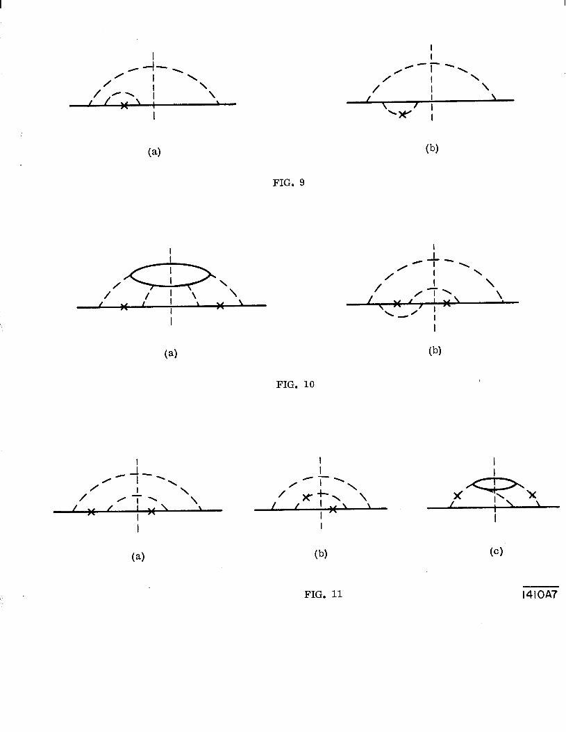


![Subjet distributions in deep inelastic …0812.2864v1 [hep-ex] 15 Dec 2008 DESY–08–178 December 2008 Subjet distributions in deep inelastic scattering at HERA ZEUS Collaboration](https://static.documents.pub/doc/80x56/5ae0ea1a7f8b9a97518dd60e/subjet-distributions-in-deep-inelastic-08122864v1-hep-ex-15-dec-2008-desy08178.jpg)


