Sequential Multiple Assignment Randomization Trials …yl2802/SMARTer.pdf · Sequential Multiple...

Sequential Multiple Assignment Randomization Trials with Enrichment Design 1

Sequential Multiple Assignment Randomization Trials with Enrichment Design

Ying Liu

Department of Biostatistics, Columbia University, NY,USA

email: [email protected]

and

Yuanjia Wang

Department of Biostatistics, Columbia University, NY, USA.


and

Donglin Zeng

Department of Biostatistics, University of North Carolina at Chapel Hill, NC, USA


Summary: Sequential multiple assignment randomization trial (SMART) is a powerful design to study Dynamic

Treatment Regimes (DTRs) and allows causal comparisons of DTRs.To handle practical challenges of SMART study,

we propose a SMART with Enrichment (SMARTer) design, which can potentially improve the design efficiency,

shorten the recruitment period, and reduce the trial duration to make SMART more practical with limited time

and resource. Specifically, at each subsequent stage of a SMART, we enrich the study sample with new patients

who have received previous stages’ treatments in a naturalistic fashion without randomization, and only randomize

them among the current stage treatment options. One extreme case of the SMARTer is to synthesize separate

independent single-stage randomized trials with patients who have received previous stage treatments. We show data

from SMARTer allows for unbiased estimation of DTRs as SMART does under certain assumptions. Furthermore,

we show analytically that the efficiency gain of the new design over SMART can be significant especially when the

dropout rate is high. Lastly, extensive simulation studies are performed to demonstrate performance of SMARTer

design, and sample size estimation in a scenario informed by real data from a SMART study is presented.

Biometrics 000, 000–000 DOI: 000

000 0000

Key words: SMART; Dynamic Treatment Regimen; Clinical Trial Design; Stratification; Power Calculations;

Efficiency


1. Introduction

Dynamic Treatment Regimes (DTRs), also referred to as adaptive treatment regimes or

tailored treatment regimens, are sequential treatment rules tailored at each stage by pa-

tients’ time-varying characteristics and intermediate treatment responses (Lavori et al.,

2000; Murphy et al., 2007; Dawson and Lavori, 2004). For example, an oncologist aiming to

prolong survival for a cancer patient might use intermediate outcomes such as patient’s tumor

response to induction therapy to guide the use of second-line therapy. Sequential multiple

assignment randomization trials (SMARTs) (Lavori and Dawson, 2000, 2004; Murphy, 2005)

generalize conventional randomized clinical trials to make causal comparisons of such DTRs.

In SMARTs, patients are randomized to different treatments at each critical decision stage,

where randomization probabilities may depend on patients’ time-varying information up to

that stage. These trials also provide rich information to infer optimal treatment regimes

tailored to individual patients. Murphy (Murphy, 2005) provides inferences and sample size

formula to compare two DTRs in SMARTs, Almirall et al. (Almirall et al., 2012) proposed

to use SMART design as a pilot study for building effective DTRs, and Nahum-Shani et al.

(Nahum-Shani et al., 2012) illustrated several important design issues and primary analyses

for SMART studies.

We use a real study (Kasari et al., 2014) to illustrate DTR and concepts in SMART.

Kasari et al. (2014) conducted a SMART on communication intervention for minimal verbally

children with autism. The study is a two-stage SMART targeted on testing the effect of a

speech-generating device (SGD). In the first stage, 61 children were randomized to a blended

developmental/behavioral intervention (JASP+EMT) with or without augmentation of a

SGD for 12 weeks with equal probability. At the end of the 12th week, children were assessed

for early response versus slow response to stage 1 treatment. In the second stage, the early-

responders continued with the first stage treatments. The slow-responders to (JASP+EMT)

2 Biometrics, 000 0000

were randomized to (JASP+EMT+SGD) or intensified (JASP+EMT+SGD) with equal

probability. The second stage lasted 12 weeks and followed by a follow up stage of 12

weeks. In this study, the primary aim was to compare the first stage treatment options SGD

(JASP+EMT+SGD) verses spoken words alone (JASP+EMT). Secondary aim was to com-

pare the dynamic treatment regimes (DTRs), namely: 1. beginning with JASP+EMT+SGD

and intensifying JASP+EMT+SGD for slow responders; 2 beginning with JASP+EMT and

to increase the intensity for slow responders; 3. beginning with JASP+EMT and to switch

JASP+EMT+SGD for slow responders.

Study dropout is a common phenomenon in randomized clinical trials (RCTs) regardless of

investigator’s best efforts to keep patients in the study. For example, meta analyses of study

dropout rate for RCTs of antipsychotic drugs reported an average attrition rate of greater

than 30% (Martin et al., 2006; Kemmler et al., 2005). For multi-stage SMARTs, even higher

dropout rate might be expected. Although smaller SMARTs maybe have lower drop out rate

(e.g., 15% in Kasari et al., 2014), attrition is still an issue not to be ignored in the planning

stage. In the Clinical Antipsychotic Trials of Intervention and Effectiveness (CATIE) study

(Schneider et al., 2003), the attrition was high with 705 of 1460 patients (48%) staying for the

entire 18 months. In a two-stage randomized trial on induction chemotherapies followed by

maintenance chemotherapy with or without radiotherapy to the chest (Joss et al., 1994), only

118 of 266 patients (44%) entered the second stage randomization. Designing a SMART may

thus require a larger sample size in the initial stage to ensure sufficient power for comparing

DTRs in a multi-stage trial. In addition, it is time-consuming and challenging to manage

and monitor a sequential multi-stage trial with a large sample size and long follow-up time.

The time and resource constraints may limit the ability of SMART studies to answer many

important clinical questions regarding DTRs.

In this work, we propose an innovative design and a meta-analytic approach to enrich


SMART sample and to synthesize single-stage trials without sacrificing the central feature

of SMART to make causal conclusions. We show that the proposed SMART with Enrichment

design (SMARTer) and its appropriate analysis method significantly boost the efficiency

of SMART, address the attrition issue from the design and analysis perspective, improve

practicability of SMART, and avoid pitfalls of incorrect inference on long term DTR effect

when combining single-stage randomized trials. Specifically, the proposed methodology can

potentially (1) extract information from patients dropping out from the first stage; (2)

recruit and randomize additional patients to the second-stage treatments without requiring

randomization of the first-stage treatments, and thus achieve the same or superior efficiency

as if there were no dropouts, which reduces the sample size of the initial stage and the overall

sample size; and (3) synthesize single-stage trials to integrate information to make causal

inference on DTRs as is possible in a multi-stage SMART, while substantially shortening

the trial time frame.

It is of interest to note that the proposed SMARTer design differs from an intuitive

approach that pieces together results from separate randomized trials conducted at separate

stages, as criticized in previous literature (Murphy et al., 2007; Collins et al., 2014). For the

latter, an investigator may determine the best first-line treatment based on a conventional

randomized trial comparing several first-line treatments and then next, compare second-line

treatments for a new group of subjects already treated by the “best” first-stage treatment.

Essentially, this intuitive approach compares available intervention options at each stage

separately to infer the best DTR. It has several disadvantages (Murphy et al., 2007): first,

it does not capture the delayed effect when the long term effect begins to appear in latter

stages; second, it fails to take into account the prescriptive effect of an early stage treatment

which may not yield a larger intermediate outcome; third, single-stage trials tend to enroll

more homogeneous patients to increase power for detection of treatment differences whereas


SMART would not. In terms of design, SMARTer does not recommend enriching the

sample with only the subjects who have received the “best” first-line treatment inferred

from a single-stage trial. Instead, we recruit enrichment samples from subjects who have

received any of the first-line treatments so that the enrich population includes patients

with all possible combinations of both lines of treatments to properly account for delayed

effect and prescriptive effect. The main focus of SMARTer design is to improve efficiency

through enrichment samples who only receive randomization in the latter stages. In terms

of the analysis, instead of inferring the best treatment from each single stage separately,

SMARTer can infer optimal DTRs with backward induction algorithms such as Q-learning

(Murphy et al., 2007), which uses the randomized samples for each stage including the

enrichment participants.

This paper is structured as follows. In Section 2, we introduce SMARTer design and

justify the validity under a causal inference framework. In Section 3, we provide the esti-

mation and inference for estimating the mean outcome of a DTR and comparison of two

DTRs. In Section 4, we study the efficiency of SMARTer as compared to SMART and

compare their sample sizes. Extensive simulation study results are shown in Section 5 to

examine the performance of SMARTer, the accuracy of the derived sample size formula,

and the robustness of this design. In section 6, we illustrate the sample size calculation

under design parameters informed by a real world SMART study of autism disorder. Section

7 provides some preliminary work of finding the optimal DTR based on a SMARTer design

and concludes with some discussions.


2. SMARTer Design

2.1 Rationales of the SMARTer Design

The essential idea of a SMARTer design is that at the kth stage (k > 1), enrich the original

SMART with new patients randomized among the kth stage treatment options. As illustrated

in the flowchart Figure 1, consider enrichment for a two-stage SMART with no intermediate

outcomes. Generalizations to more than two stages and including intermediate outcomes

are similar. Assume that n patients are randomized at the first stage in a SMART. Some

patients complete the first stage treatment and undergo the second stage randomization

(group 1), while some patients drop out before the second stage randomization (group 2). To

mitigate the problem of attrition after the first stage treatment, while the original SMART

is progressing, we concurrently recruit m new patients as the enrichment sample (group 3).

One key eligibility criterion for the enrichment group is that they have received one of the

first stage treatments. However, their first stage treatments can be assigned in a naturalist

fashion without randomization prior to the enrollment. For the enrichment subjects in group

3, their second-stage treatments will be randomized as in the original SMART.

Taking the autism study (Kasari et al., 2014) as an example, the primary outcome for

this study was the total number of spontaneous communicative utterances (TSCU). The

response status to the first stage treatment was the intermediate outcome that the second

stage treatment choice and randomization probability depended on. For example, for a DTR

starting with JASP+EMT, whether a patient participates in the second randomization to

add SGD or intensify depends on whether he/she is a slow responder or not. Group 1 patients

would be those who were randomized in the first stage and stayed through the trial until

the end of the second stage. Group 2 patients include the 6 patients who dropped out

after randomization in the first stage, and the additional 3 patients who dropped out after

finishing first stage and on whom the intermediate response variables were recorded. In the


next few sections, we will provide analysis of efficiency and sample size computation for the

enrichment group 3 patients in the new SMARTer design to estimate the mean outcome

of a given DTR and compare DTRs.

The final analysis sample of SMARTer consists of three groups of patients (also shown

in Figure 1). Specifically, group 1 is the n1 SMART subjects who stay through two stages

of randomization and treatments; group 2 is the n2 SMART subjects who drop out before

the second randomization; and group 3 is the m enrichment subjects who only receive the

second-stage randomization with known first-stage treatment history. Let Zi denote the

indicator of stage 2 completion status for subject i, Si denote pre-treatment information

at stage 1, Aki denote treatment at stage k (k = 1, 2), and Yi denote the observed reward

outcome from the study. Then SMARTer data consist of the data from the original SMART

subjects, (Si, A1i, ZiA2i, ZiYi, i = 1, ..., n), and the data from the m enrichment subjects,

(Sj, A1j, A2j, Yj, j = 1, ...,m). In the subsequent presentation, we assume Si to take a finite

number of discrete values for convenience.

[Figure 1 about here.]

To understand why SMARTer enables valid evaluation of DTRs under certain assump-

tions, we first focus on a two-stage trial and assume that there is no intermediate information

after stage 1. For any DTR (d1, d2), a sequence of decision rules with dk representing a func-

tion mapping historical information to the domain of Ak for k = 1, 2, our goal is to estimate

the value function of (d1, d2) defined as E[Y (d1, d2)]. Here Y (a1, a2) is the potential outcome

associated with the treatment assignment (a1, a2). We assume the following conditions hold:

(C.1) Y =∑

a1,a2Y (a1, a2)I(A1 = a1, A2 = a2); (C.2) The dropout is independent of

{Y (a1, a2)} given (A1, S); (C.3) The conditional distribution of Y given (A1, S, A2) in the

enrichment group is the same as that in the original SMART population. (C.4) The first stage


domain of A1 (treatment options) for the enrichment group is identical to the treatment A1

in the SMART population.

Condition (C.1) is the standard stable unit treatment value assumption (SUTVA) in

causal inference. Condition (C.2) is the standard non-informative dropout or missing at

random (MAR) assumption also required in any analysis of an RCT. The key condition

(C.3) requires that the conditional treatment effect given S is the same between the original

SMART samples and the enrichment samples. This assumption is important since if it is not

satisfied, the data from the enrichment group cannot be used to complement the original

SMART. Condition (C.4) ensures the first stage treatments are comparable in the SMART

and enrichment samples.

Under conditions (C.1)–(C.4), we show SMARTer can provide an unbiased estimation of

the average causal outcome for the DTR (d1, d2), that is, E[Y (d1, d2)]. The essential idea is

that sequential ignorability assumption required to draw causal inference is satisfied in the

enrichment sample when used to predict mean outcomes and compare second stage treatment

options. In other words, due to sequential ignorability, potential outcomes {Y (a1, a2)} are

conditionally independent of A2 given (A1, S) in the enrichment sample, even if their first

stage treatments can be received in a naturalistic fashion without randomization. When

comparing first stage treatment options, we only use the non-dropouts from the original

SMART and predicted outcomes for n2 dropouts whose first stage treatments are random-

ized. Specifically, let pk(ak|sk) denote the randomization probability of Ak given a patient’s

covariates collected up to stage k, i.e., sk. Note that for simplicity, here we assume second

stage randomization probabilities depend on baseline covariates and first stage treatments.

In Section 2.3, we generalize to allow them to depend on intermediate outcomes. Our key

result is to show

E[Y (d1, d2)] = µ1 = µ2,


where µ1 = E1

[I(A1 = d1(S), A2 = d2(A1, S))

p1(A1|S)p2(A2|S,A1)Y

], µ2 = E2

[I(A1 = d1(S))

p1(A1|S)Y ∗],

Eg[·] denotes the expectation for subjects in group g, and Y ∗ denotes the conditional mean

of Y given (A1, S, A2 = d2(A1, S)) for subjects in group 1 and 3. The rationale is that if this

equality holds, then the average causal outcome, E[Y (d1, d2)], can be estimated unbiasedly

using the data from SMARTer since Y ∗, E1[·], and E2[·] can be estimated unbiasedly using

their corresponding empirical averages. There are three observations of this result: (1) Since

group 1 subjects’ final outcomes Y are observed, we estimate their average causal mean using

their observed outcomes; (2) Group 2 subjects drop out after first-stage and have missing

Y , but their outcomes can be estimated as Y ∗ from subjects in group 1 and 3; (3) Group 3

subjects contribute to the estimation through estimating missing outcomes for subjects in

group 2.

To see why the above equalities hold, first note that under condition (C.1), we obtain

µ1 = E1

[I(A1 = d1(S), A2 = d2(A1, S))

p1(A1|S)p2(A2|S,A1)Y (d1, d2)

].

By randomization, A2 is independent of potential outcome Y (d1, d2) given (S,A1). Thus,

since E1[·] is equivalent to E[·] under the non-informative dropout condition (C.2), the above

expression becomes

µ1 = E

[I(A1 = d1(S))

p1(A1|S)Y (d1, d2)

].

Furthermore, by randomization of A1 in the first stage for group 1 subjects, we obtain the

above equation to also equal the average causal outcome, i.e.,

µ1 = E

[E

{I(A1 = d1(S))

p1(d1|S)|S}E {Y (d1, d2)|S}

]= E[Y (d1, d2)].

Next, due to randomization of A2 for subjects in group 1 and group 3, under condition (C.3),

we obtain

Y ∗ = E[Y (A1, d2(A1, S))|A1, S, A2 = d2(A1, S)] = E[Y (A1, d2(A1, S1))|A1, S].


Consequently,

µ2 = E

[I(A1 = d1(S))

p1(A1|S)E[Y (A1, d2(A1, S))|A1, S]

]= E

[I(A1 = d1(S))

p1(A1|S)E[Y (d1, d2)|A1, S]

].

Again, by the randomization of A1 for subjects in group 2, we conclude µ2 = E[Y (d1, d2)].

2.2 Value Estimation and Inference in SMARTer

Given a DTR (d1, d2), for a patient with S = s and treatment assignment a1 = d1(s) and

a2 = d2(s, a1), an estimator of the expected outcome value associated with this DTR is

µ(d1, d2) =

{n∑i=1

(ZiI(A1i = d1(Si), A2i = d2(Si, A1i))

p(A1i|Si)p(A2i|Si, A1i)+ (1− Zi)

I(A1i = d1(Si))

p(A1i|Si)

)}−1

×

{n∑i=1

(ZiI(A1i = d1(Si), A2i = d2(Si, A1i))

p(A1i|Si)p(A2i|Si, A1i)Yi

+(1− Zi)I(A1i = d1(Si))

p(A1i|Si)Y (A1i, d2(Si, A1i), Si)

)}, (1)

where Y (a1, a2, s) is the predicted outcomes for group 2 subjects using group 1 and group 3

data:

Y (a1, a2, s) =

∑ni=1 ZiYiI(A1i = a1, A2i = a2, Si = s) +

∑mj=1 YjI(A1j = a1, A2j = a2, Sj = s)∑n

i=1 ZiI(A1i = a1, A2i = a2, Si = s) +∑m

j=1 I(A1j = a1, A2j = a2, Sj = s).

The essential idea is to compute the average outcome for subjects in SMART using observed

outcomes for group 1 and imputed outcomes for group 2 (imputed using group 1 and 3 data).

The enrichment sample improves estimation efficiency through nonparametric imputation

(simple average) for subjects in group 2. Note that from (1), even without an enrichment

sample (i.e., m = 0), we can still impute group 2 subjects’ outcomes using group 1 subjects’

to improve efficiency with no bias. Thus the estimator in (1) deals with missing data issue

for SMART design as well. It is clear that the estimator in (1) adheres to the intention-

to-treatment principal (Fisher et al., 1989) such that all subjects randomized are analyzed

according to their original treatment assignments.

Next, we derive the asymptotic variance formula for estimator (1) under the conditions

(C.1) through (C.4) assuming m = O(n). Specifically, we wish to obtain the asymptotic


expansion of µ(d1, d2) − µ(d1, d2). To this end, we let p(s) be the probability of S = s and

p(a1|s) be the randomization probability of A1 = a1 given S = s in the SMART population

in the first stage and let p(a2|s, a1) be the randomization probability of A2 = a2 given

S = s and A1 = a1 in the second stage. These two conditional probabilities are known

by design. Furthermore, we let q(s) and q(a1|s) be the probability of enrichment sample

with S = s and receiving first-stage treatment A = a1 given S = s. Note that due to the

observational nature of the enrichment group for the first-stage treatment, q(s) may not

equal p(s) and q(a1|s) may not equal p(a1|s). We let π1(a1, a2, s) = p(a2|s, a1)p(a1|s)p(s),

π2(a1, a2, s) = p(a1|s)p(s)I(d2(s, a1) = a2), and π3(a1, a2, s) = p(a2|s, a1)q(a1|s)q(s). Finally,

denote α(a1, s) = P (Z = 1|A1 = a1, S = s), β = m/n, and r(a1, s) = q(a1|s)q(s)/[p(a1|s)p(s)].

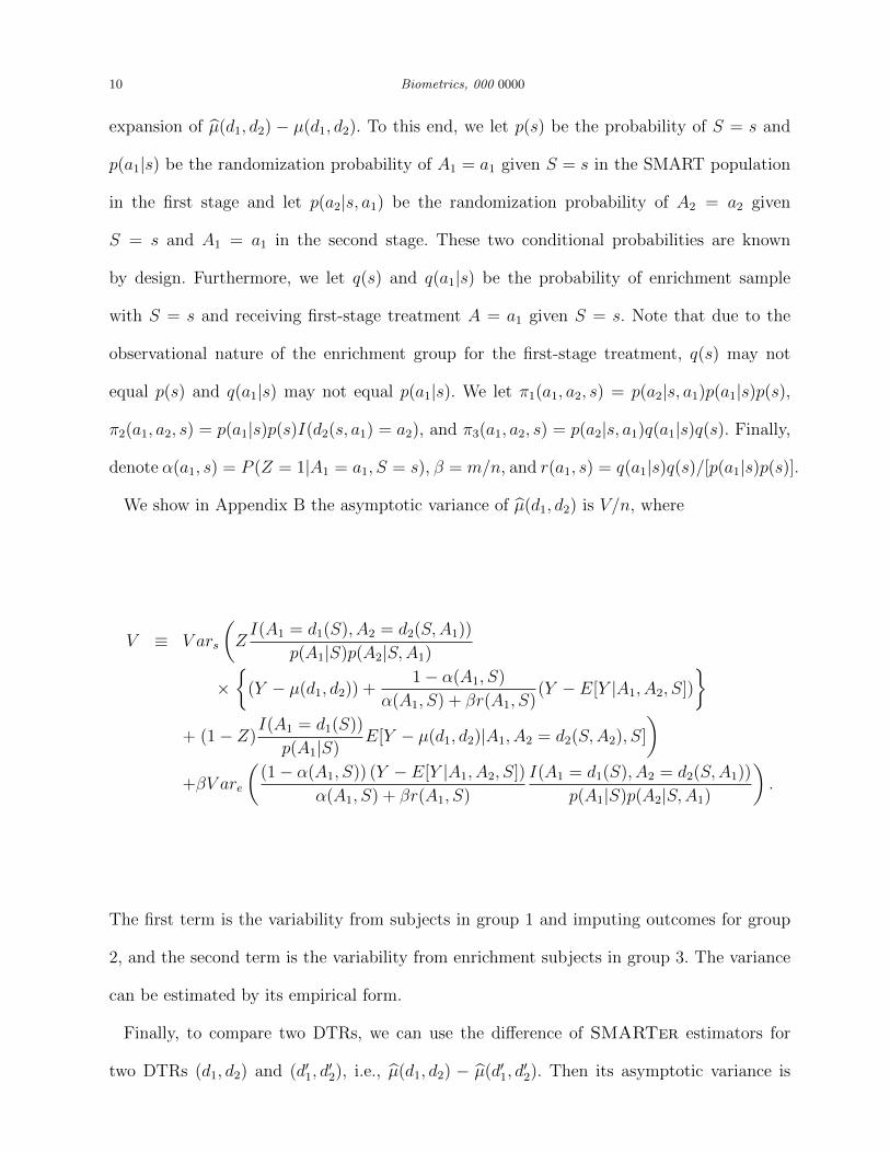
We show in Appendix B the asymptotic variance of µ(d1, d2) is V/n, where

V ≡ V ars

(ZI(A1 = d1(S), A2 = d2(S,A1))

p(A1|S)p(A2|S,A1)

×{

(Y − µ(d1, d2)) +1− α(A1, S)

α(A1, S) + βr(A1, S)(Y − E[Y |A1, A2, S])

}+ (1− Z)

I(A1 = d1(S))

p(A1|S)E[Y − µ(d1, d2)|A1, A2 = d2(S,A2), S]

)+βV are

((1− α(A1, S)) (Y − E[Y |A1, A2, S])

α(A1, S) + βr(A1, S)

I(A1 = d1(S), A2 = d2(S,A1))

p(A1|S)p(A2|S,A1)

).

The first term is the variability from subjects in group 1 and imputing outcomes for group

2, and the second term is the variability from enrichment subjects in group 3. The variance

can be estimated by its empirical form.

Finally, to compare two DTRs, we can use the difference of SMARTer estimators for

two DTRs (d1, d2) and (d′1, d′2), i.e., µ(d1, d2) − µ(d′1, d

′2). Then its asymptotic variance is


V (d2, d′2)/n, where

V (d2, d′2)

≡ V ars

{ZI(A1 = d1(S), A2 = d2(S,A1))

p(A1|S)p(A2|S,A1)

×(

(Y − µ(d1, d2)) +1− α(A1, S)

α(A1, S) + βr(A1, S)(Y − E[Y |A1, A2, S])

)−Z I(A1 = d′1(S), A2 = d′2(S,A1))

p(A1|S)p(A2|S,A1)

×(

(Y − µ(d′1, d′2)) +

1− α(A1, S)

α(A1, S) + βr(A1, S)(Y − E[Y |A1, A2, S])

)+ (1− Z)

I(A1 = d1(S))

p(A1|S)E[Y − µ(d1, d2)|A1, A2 = d2(S,A2), S]

− (1− Z)I(A1 = d′1(S))

p(A1|S)E[Y − µ(d′1, d

′2)|A1, A2 = d′2(S,A2), S]

}+βV are

[(1− α(A1, S)) (Y − E[Y |A1, A2, S])

α(A1, S) + βr(A1, S)

I(A1 = d1, A2 = d2)− I(A1 = d′1, A2 = d′2)

p(A1|S)p(A2|S,A1)

].

This variance can also be estimated by its empirical form.

2.3 Incorporating intermediate outcomes

The previous section assumes no intermediate outcome is available especially for subjects who

drop out from the SMART. When intermediate outcomes on these subjects are available, con-

sider the DTR (d1, d2), where the treatment rule d2 may depend on the intermediate outcome.

In this case, the observed data from a SMARTer consist of (S1i, A1i, S2i, ZiA2i, ZiYi), i =

1, ..., n, for i in the original SMART group, and the enrichment group observations

(S1j, A1j, S2j, A2j, Yj), j = 1, ...,m. Here, we use S1 to denote pre-treatment covariates at

stage 1 and S2 to denote intermediate outcomes and other covariates collected prior to stage 2.

For simplicity of derivation, we assume S1i and S2j to be discrete. Similar to (1), a consistent

estimator of the associated value using both the SMART and enrichment observations is


µ(d1, d2) =

{n∑i=1

(ZiI(A1i = d1(S1i), A2i = d2(S1i, A1i, S2i))

p(A1i|S1i)p(A2i|S1i, A1i, S2i)+ (1− Zi)

I(A1i = d1(S1i))

p(A1i|S1i)

)}−1

×

{n∑i=1

(Zi

I(A1i = d1(S1i), A2i = d2))

p(A1i|S1i)p(A2i|S1i, A1i, S2i)Yi

+(1− Zi)I(A1i = d1(S1i))

p(A1i|S1i)Y (A1i, d2(S1i, A1i, S2i), S1i, S2i)

)},

where Y (a1, a2, s) is the imputed outcome from the second-stage data given asn∑i=1

ZiYiI(A1i = a1, A2i = a2, S1i = s1, S2i = s2) +m∑j=1

YjI(A1j = a1, A2j = a2, S1j = s1, S2j = s2)

n∑i=1

ZiI(A1i = a1, A2i = a2, S1i = s1, S2i = s2) +m∑j=1

I(A1j = a1, A2j = a2, S1j = s1, S2j = s2).

The asymptotic variance is similar to before by re-defining πk(a1, a2, s) as πk(a1, a2, s1, s2)

through conditioning on both the baseline covariates S1 and intermediate outcome S2. That

is,

V ≡ V ars

(ZI(A1 = d1(S1), A2 = d2(S1, A1, S2))

p(A1|S1)p(A2|S1, A1, S2)

×{

(Y − µ(d1, d2)) +1− α(A1, S1, S2)

α(A1, S1, S2) + βr(A1, S1, S2)(Y − E[Y |A1, A2, S1, S2])

}+ (1− Z)

I(A1 = d1(S1))

p(A1|S1)E[Y − µ(d1, d2)|A1, A2 = d2(S1, A2, S2), S1]

)+βV are

((1− α(A1, S1, S2)) (Y − E[Y |A1, A2, S1, S2])

α(A1, S) + βr(A1, S1, S2)

I(A1 = d1(S1), A2 = d2(S1, A1, S2))

p(A1|S1)p(A2|S1, A1, S2)

).

3. Design Efficiency of SMARTer

In this section, we study the efficiency gain or loss of the proposed design as compared

to a SMART with no dropout. For simplicity of illustration, we assume P (Z = 1|A1, S)

to be a constant, i.e., α(a1, s) = α, and let ω(s) = r(d1(s), s). Furthermore, we denote

p(d1(s)|s) = p1(s) and p(d2(s, d1(s))|d1(s), s) = p2(s), so the variance of µ(d1, d2) is V/n

with


V = Es

[(α

p1(S)p2(S)+

1− αp1(S)

)(ν(S)− µ(d1, d2))2

]+Es

[σ(S)2

p1(S)p2(S)

α(1 + βω(S))2 + β(1− α)2ω(S)

(α + βω(S))2

],

where Es[·] is the expectation with respect to S in the SMART population,

ν(s) = Es(Y |A1 = d1(s), A2 = d2(d1(s), s), S = s) = Ee(Y |A1 = d1(s), A2 = d2(d1(s), s), S = s),

and σ(s)2 = V ars(Y |A1 = d1(s), A2 = d2(d1(s), s), S = s)

= V are(Y |A1 = d1(s), A2 = d2(d1(s), s), S = s).

When α = 1, i.e., no participant drops out from SMART, V reduces to

V0 = Es

[(ν(S)− µ(d1, d2))2 + σ(S)2

p1(S)p2(S)

],

which is the variance formula given in Murphy (2005) for SMART. Therefore, to measure

the efficiency gain of the proposed design over SMART design without dropouts, we define

relative efficiency ρ = V0/V , where ρ > 1 implies the propose enrichment design is more

efficient than the original SMART without dropout.

To further gain insights on efficiency comparison, we consider a special situation when

treatment randomization does not depend on tailoring variables, i.e., p1(S) = p1, p2(S) = p2.

We also assume that the enrichment population is close to the original SMART population

so ω(s) ≈ 1, and let the ratio of within- and between-strata variance to be γ ≈ σ(s)2/(ν(s)−

µ(d1, d2))2. Let α denote the completion (non-dropout) rate, and β = m/n denote the

enrichment rate. We can show that

ρ ≈ 1 + γ

1− (1− α)(1− p2) + γ α(1+β)2+β(1−α)2

(α+β)2

. (2)

From (2), the relative efficiency depends on randomization probabilities, within- and between-

strata (S) variability and distribution ratios between the enrichment and SMART popula-

tions. Note that ρ > 1 implies the proposed SMARTer is more efficient than a SMART


without enrichment and no dropout. From the expression of ρ, we thus conclude:

(1) When α = 1, there is no dropout after the first stage in SMARTer, our estimator

reduces to be the same as the estimator in Murphy (2005), and thus ρ = 1.

(2) When α = 0, that is, all subjects drop out after the first stage, ρ ≈ (1 + γ)/(p2 + γ/β).

There is efficiency gain if β > γ/(1+γ−p2). More specifically, there is always efficiency gain

if β > 1. Note that this is the extreme case in the sense that all subjects drop out and we

synthesize two independent randomized trials on the two stages.

(3) For any 0 < α < 1 , if α(1 + β)2 + β(1 − α)2 6 (α + β)2, ρ > 1 implies efficiency gain.

Particularly, the latter condition holds if we choose β > 1.

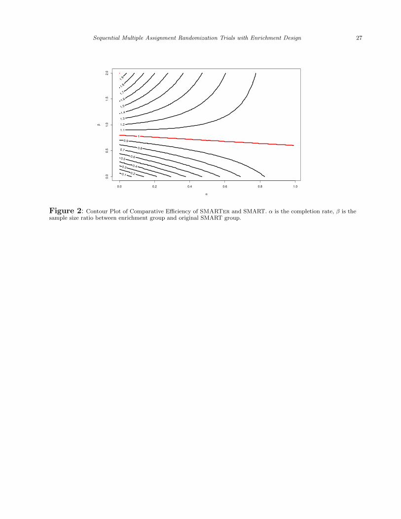
Figure 2 is the contour plot of ρ as a function of completion (non-dropout) rate α and the

enrichment rate β = m/n under γ = 0.5, 2, where each line represents the contour line of

the marked relative efficiency ρ as defined above. For example, for the ρ = 0.9 line, α = 0.6

corresponds to β = 0.5. That is, at 60% completion rate, a study needs to enrich 50%

sample to obtain a SMARTer estimator with variance 1/0.9 ≈ 1.11 times the variance of

SMART estimator with the same initial sample size but no dropout. Similarly, at the same

completion rate, to achieve the same efficiency, β needs to be above 0.75; and to achieve a

relative efficiency of ρ = 1.1, β need to be above 1.05. Note that the line with equal efficiency

has a slow change rate indicating the increase of enrichment sample size is not sensitive to

completion rate. The contour lines above the equal efficiency line (ρ = 1) are convex and

increasing, indicating with lower dropout rate after the first stage, SMARTer requires

more enrichment patients at the second stage to achieve higher efficiency than a SMART

with no dropout. The opposite can be seen from the contour lines below the equal efficiency

line which are concave and decreasing: with lower dropout rate, SMARTer requires less

enrichment patients or no enrichment to achieve efficiency slightly lower than a SMART with

no dropout.


[Figure 2 about here.]

Another way to understand the design efficiency of SMARTer is through sample size

calculation for comparing two DTRs in a SMARTer study. We denote the difference in the

mean outcome value as ∆µ and assume the type I error rate of a two-sided test is 0.05 and

80% power to detect a difference. In the above simplified setting, the total sample size of

SMARTer is 8(z0.05/2+z0.2)2 σ2(d2)

(∆µ)2, where σ2(d2) = var(Y |A2 = d2), and zq represents the q-

th upper quantile of a standard normal distribution. With a completion rate of α, the sample

size of SMART inflates to 8(z0.05/2 + zβ)2 σ2(d2)α(∆µ)2

to ensure sufficient power at the end of the

second stage. For two DTRs with different first stage treatments, i.e., d1(S) 6= d′1(S) for any

S, one can compute the variance of the difference as V (d2, d′2) = V (d2) + V (d′2). Assuming

σ2(d2) = σ2(d′2), then ρ is also the ratio of variance of SMART and SMARTer estimator

for comparing two DTRs. Thus the sample size of initial recruitment (n) for a SMARTer

is 8(z0.05/2 + zβ)2 σ2

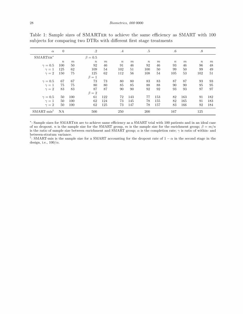
(∆µ)2ρto achieve the same efficiency. Table 1 provides the sample sizes for

a SMARTer with an initial sample of n subjects and an enrichment sample of m subjects

to achieve the same efficiency as a SMART recruiting 100 subjects and in an ideal case of

no dropout. For example, if 40% patients drop out after the first stage randomization of

SMARTer and the within- and between- stratum variance ratio γ = 1, Table 1 provides

three combinations of initial stage and enrichment sample sizes for SMARTer to achieve the

same efficiency: (109, 54), (80, 80) and (62, 124). In contrast, when accounting for dropouts

at the design stage for a SMART without enrichment, one needs 100/0.6=250 subjects.

4. Simulation Studies

Simulations results are based on 1000 replications of samples with initial enrollment of n =

800 patients. They demonstrate the consistency and comparative efficiency of SMARTer

compared with SMART under various scenarios with or without intermediate outcomes.


4.1 Simulation Results without Intermediate Outcomes

Here we assume there are two stages each with 2 candidate treatments, A1 and A2, and

a randomization probability of 1/2. The baseline covariate S1 takes random integer values

(0, 1, 2) with probabilities (1/3, 1/3, 1/3). Let S2 = A1(1 − S1), and the final outcome after

the second stage is Y = S2 +A2(1−S1)+I(S1 = 1, A1 = 1, A2 = −1)+e, where e ∼ N (0, 1).

The optimal dynamic rules for this setting are d1(S1) = 2I(S1 < 2) − 1 and d2(S1, A1) =

2I(S1 < 1) − 1. Under this rule ν(S1 = 0) = 2, ν(S1 = 1) = 1, ν(S1 = 2) = 2, thus the

optimal rule has a value of µ(d1, d2) = 1.667. We consider two levels of completion rates

α = 0, 0.5, three levels of enrichment proportions β = 0.5, 1, 2 and two scenarios for the m

enrichment patients with the baseline distribution of q = (1/2, 1/4, 1/4) for S1: scenario 1

simulates the distribution of A1 for the enrichment patients the same as initially recruited

patients, i.e., q(A1|S1) = p(A1|S1) = 1/2; and scenario 2 simulates different observed A1

distribution q(A1 = 1|S1) = 1/(1 + exp(−0.5(2I(S1 < 2) − 1))), that is, the enrichment

patients are more likely to receive the optimal first-stage treatment.

Table 3 presents SMARTer estimators of a single DTR and comparison of two DTRs,

as well as their efficiency gain (ρ) compared with SMART without dropout. We provide

the estimates for the optimal treatment regime d1(S1) = 2I(S1 < 2) − 1 and d2(S1, A1) =

2I(S1 < 1) − 1, and its comparison with an one-size-fits-all regime, d′1(S1, A1) = −1 and

d′2(S1, A1) = 1, for which the mean outcome is µ′ = 0.

The results show the accuracy of the variance estimation and the simplified formula (2) of

comparative efficiency. When all patients drop out (α = 0), the relative efficiency ρ increases

from about 0.5 to 2 when the enrichment size m increases from 0.5 to 2 times the original

sample size n; when half of patients drop out (α = 0.5), the relative efficiency ρ increases from

about 0.9 to 1.3. As β increases, SMARTer is more efficient comparing to SMART design

even when all patients drops out after the initial randomization (α = 0) and SMARTer


combines two single-stage randomized trials. We also observe that the relative efficiency ρ

for comparing two DTRs is greater (more efficient) than estimating a single DTR.

4.2 Simulation Results with Intermediate Outcomes

The general settings are the same with section 5.1. The intermediate outcome before the sec-

ond stage treatment S2 is simulated from a logistic model, where logit{P (S2 = 1|A1, S1)} =

A1(1 − S1), and the outcome after the second stage treatment is Y = S2 + A2(1 − X) +

I(X = 1)A2(2S2 − 1) + e, where e ∼ N (0, 1). The dynamic rules we are considering is

the optimal rule under this scenario, which also depends on the intermediate outcome S2:

d1(S1, A1) = 2I(S1 = 1)−1 and d2(S1) = I(S1 6= 1)(2I(S1 = 0)−1)+I(S1 = 1)sign(2S2−1).

Under this rule ν(S1 = 0) = 1 + e1+e

, ν(S1 = 1) = 1.5, ν(S1 = 2) = 1 + e1+e

. Thus the mean

outcome for the optimal rule is µ(d1, d2) = 1.654 with equal baseline distribution for S1.

Table 3 presents SMARTer estimators of both a single DTR and comparison of two DTRs,

as well as their efficiency gain (ρ) compared with SMART estimator with no dropout. We

present the estimates for the optimal DTR and its comparison with an one-size-fits-all rule:

d′1(S1, A1) = −1 and d′2(S1, A1, S2) = 1, for which the mean outcome is µ′ = 0.5. The true

mean difference is 1.154. The results are similar to the case without intermediate outcome.

When β = 1, ρ is approximately equal or larger than 1, and it is higher for the difference

comparison in Table 4. We observe that SMARTer estimator has efficiency gain even with

β = 1 and it may boost efficiency especially when comparing two DTRs.

5. Sample size calculation for an Autism SMART study

We illustrate the sample size calculation and potential efficiency gain using results from the

autism study (Kasari et al., 2014) introduced in Section 2.1. For the primary aim, they study

found that SGD(JASP+EMT+SGD) has a better treatment effect compared with spoken

words alone (JASP+EMT). Secondary aim results suggest that the adaptive intervention


beginning with JASP+EMT+SGD and intensifying JASP+EMT+SGD for children who

were slow responders led to better post-treatment outcomes.

Suppose we stratify by baseline variables and responding status (early or slow) after the

first stage. Here we provide the sample size calculation for comparing two adaptive treatment

regimes as in the secondary study aim: one is starting with JASP+EMT+SGD and inten-

sifying JASP+EMT+SGD for children who are slow responders (d2); the other is starting

with JASP+EMT, and the slow-responders to JASP+EMT receive JASP+EMT+SGD (d′2).

The original planned sample size was based on the primary aim to compare TSCU for

two treatments in stage 1. The study assumed an attrition rate of 10% by week 24, and the

planned total sample size was n = 97 to detect a moderate effect size of 0.6 in TSCU with

80% power using a two-sided two-sample t-test with a type I error rate of 5%. The actual

study recruited 61 patients. The effect size for the primary aim comparison was 0.62 and it

was significant at 0.05 level despite the insufficient power. As a secondary aim of the study,

the effect size of the embedded DTRs d2 and d′2 for TSCU at week 24 was 0.55. There were

approximately 15% patients dropped out after the first stage at week 12. The comparison

of two DTRs in the secondary aim had approximately a power of 37% to detect a moderate

effect size of 0.5.

We examine whether one can design a SMARTer to enrich the trial in the second stage

so that the power for comparing two DTRs can be improved. To this end, note the following

holds Zβ 6 ∆µη/n

, where ∆µ is the effect size, and η = (V (d2) +V (d′2))/σ2 = 4+0.8αγ+1

+ 4.8γ1+γ

1+αβα+β

.

When γ = 0.5, we have Zβ 6 −0.115 and we can achieve at most 55% in power by enrichment

in the second stage. To achieve 80% power, one needs to at least recruit 151 patients in the

first stage.

Table 2 provides sample sizes for SMARTer and SMART that achieve the same power of

90%, 85% or 80% for two-sided tests with a type I error rate of 5%. The sample size for initial


stage of SMARTer is computed by n =(2+2×0.6+4×0.4)(Zα/2+Zβ)2

∆µ2, where we take into account

d2 was randomized only in the first stage and for d′2, only the 40% slow responders received

two-stages of randomization. The enrichment ratio β is computed by solving V (d2)+V (d′2) =

V0(d2)+V (d′2) (by independence of subjects following d2 and d′2), that is, to solve the following

equation 11+γ

(2 + 2(1−α) + (2× 0.6 + 4× 0.4)α) + γ1+γ

(2 + 2.8)1+αβα+β

= 2 + 2.8. The solution

is β = 6γ−α6γ+1

.

Since we do not have information on the ratio of within and between stratum variances γ,

we provide results for three ratios γ = 0.2, 0.5, 1 and also two rates of attrition 15% and 40%

after the first stage. According to Table 2, for this specific example, SMARTer would have

smaller total sample size for initial recruitment and enrichment when γ is small (γ = 0.2)

with attrition rate 15% and for γ = 0.5 with attrition rate 40%. SMARTer would be more

beneficial for smaller sample sizes and when both groups being compared receive two stages

of randomization.

6. Discussion

We propose a SMARTer design to improve efficiency over SMART by enriching study

participants at each stage of a multi-stage trial. We have shown that the new design retains

the validity of making causal inference for DTRs and the efficiency gain is significant if drop

out rate is considerable and the enrichment sample size is substantial. In all numeral results,

we compared efficiency of SMARTer to SMART with no dropout. When comparing with

SMART accounting for dropouts, the efficiency gain is expected to be greater than that

shown here. One interesting application of SMARTer design is the extreme case when

α = 0, so the proposed design is equivalent to synthesizing different independent trials

from each stage. One important implication is that if the conditions (C.1)–(C.4) hold, i.e.,

the treatment response profiles are the same for the participants from each stage and the


treatment history in previous stages of the enrichment sample can be obtained, then we no

longer need to conduct a full SMART in order to evaluate DTRs. Therefore, in practice, it

may be possible to synthesize existing trials conducted at separate stages to compare DTRs,

at least for the purpose of discovering optimal DTRs. At the other extreme, when there is

no attrition (i.e., α = 1) SMARTer can still be used to gain efficiency by replacing Yi

in µ(d1, d2) by the corresponding stratum mean estimated from the combined SMART and

enrichment sample, which is less variable.

Data collected from the SMARTer can also be used to find optimal DTR using methods

such as Q-learning (Murphy et al., 2007; Watkins, 1989). Using a two-stage design as an

example, first one can find the optimal second stage treatment using the subjects randomized

at the second stage, which includes n1 group 1 subjects and the m group 3 enrichment

subjects. Next, one can use the regression model in Q-learning from this step to predict

the optimal outcomes of the group 2 dropout subjects and identify optimal second stage

treatment. Lastly, group 1 and 2 subjects are used to estimate the optimal treatment rule

for the first stage. More details on how to estimate the optimal rule and a simulation study

are included in the Web Appendix B.

Unmeasured confounding may be a concern in statistical inference using enrichment group

observational data. However, note that the enrichment sample is only used to predict out-

comes for those who drop out from the original SMART group randomized for the first

stage treatments. The enrichment samples are not directly included in the comparisons of

the DTRs. The second stage treatment options for enrichment sample are randomized and

they are matched with the SMART group based on health information collected right before

second stage randomization (including intermediate outcomes). Thus under the assumption

(C.2) of missing at random and assumption (C.3) of the same conditional distribution given

health information up to stage 2, valid inference can be drawn by predicting SMART drop out


subjects using enrichment sample. When dropout patterns are complicated and depend on

many intermediate outcomes, our simple estimation by stratification and matching may need

to be improved. A straightforward modification is instead of matching on all stratification

variables, select enrichment sample with matched cumulative summaries of main variables

(e.g., same number of interim outcome measures). Other model based methods or doubly

robust estimation may be considered for more complex situations especially when auxiliary

variables are available for estimating missingness.

From the real data example in Section 6, we see that although enrichment can improve

the power for comparing DTRs, the maximal power one can attain still depends on the

sample size in the first stage recruitment. Recruiting an enrichment sample can decrease the

within-stratum variation but can not decrease the variation from between-stratum variation.

Therefore, in reality practitioners may design a SMART with a sample size assuming a small

drop out after the first stage, and consider enriching the study sample at the second stage to

achieve the predetermined power if the actual observed dropout rate is high during the first

stage of treatment. In this case, SMARTer may act as a salvage design to mitigate high

drop out rate. In addition, one major reason for the low participation rate in clinical trials

and high attrition is the need for frequent in-person visits and the resulting time and travel

costs (Ross et al., 1999), which can be reduced for the enrichment samples in SMARTer

since these participants have already received first stage treatments. For the enrichment

sample, the cost of monitoring first stage treatment is saved, and the duration of trial for

this group can be considerably less than recruiting patients in the first stage to under go

multiple randomizations. The chance to retain participants in the trial can be much higher.

Finally, from a design point of view, although we allow the distribution of first-stage

treatment history and covariates on the enrichment participants to be different from the

SMART population, the more similar they are, the more efficiency we will gain by using the


enrichment participants. This implies that when recruiting enrichment patients for the second

stage treatments, similar inclusion/exclusion criteria as SMART may be used and certain

sampling design may be implemented to improve matching. Furthermore, since SMARTer

requires the treatment responses between the enrichment and SMART population to have

the same distributions, caution should be taken when one suspects that the two populations

may have different response mechanisms to treatments. Sensitivity analysis can be conducted

in the analysis phase.

7. Web Appendix

In the web appendix, we provide derivation of the asymptotic variance of the estimator for

expected outcome under a given DTR, as well as description and preliminary simulation

results for learning the optimal DTR from SMARTer.

References

Almirall, D., Compton, S. N., Gunlicks-Stoessel, M., Duan, N., and Murphy, S. A. (2012).

Designing a pilot sequential multiple assignment randomized trial for developing an

adaptive treatment strategy. Statistics in medicine 31, 1887–1902.

Collins, L. M., Nahum-Shani, I., and Almirall, D. (2014). Optimization of behavioral

dynamic treatment regimens based on the sequential, multiple assignment, randomized

trial (smart). Clinical Trials page 1740774514536795.

Dawson, R. and Lavori, P. W. (2004). Placebo-free designs for evaluating new mental health

treatments: the use of adaptive treatment strategies. Statistics in medicine 23, 3249–

3262.

Fisher, L., Dixon, D., Herson, J., Frankowski, R., Hearron, M., and Peace, K. E. (1989).

Intention to treat in clinical trials.

Joss, R., Alberto, P., Bleher, E., Ludwig, C., Siegenthaler, P., Martinelli, G., Sauter, C.,


Schatzmann, E., Senn, H., et al. (1994). Combined-modality treatment of small-cell

lung cancer: Randomized comparison of three induction chemotherapies followed by

maintenance chemotherapy with or without radiotherapy to the chest. Annals of oncology

5, 921–928.

Kasari, C., Kaiser, A., Goods, K., Nietfeld, J., Mathy, P., Landa, R., Murphy, S., and

Almirall, D. (2014). Communication interventions for minimally verbal children with

autism: a sequential multiple assignment randomized trial. Journal of the American

Academy of Child & Adolescent Psychiatry 53, 635–646.

Kemmler, G., Hummer, M., Widschwendter, C., and Fleischhacker, W. W. (2005). Dropout

rates in placebo-controlled and active-control clinical trials of antipsychotic drugs: a

meta-analysis. Archives of general psychiatry 62, 1305–1312.

Lavori, P. W. and Dawson, R. (2000). A design for testing clinical strategies: biased

adaptive within-subject randomization. Journal of the Royal Statistical Society: Series

A (Statistics in Society) 163, 29–38.

Lavori, P. W. and Dawson, R. (2004). Dynamic treatment regimes: practical design

considerations. Clinical trials 1, 9–20.

Lavori, P. W., Dawson, R., and Rush, A. J. (2000). Flexible treatment strategies in chronic

disease: clinical and research implications. Biological Psychiatry 48, 605–614.

Martin, J. L. R., Perez, V., Sacristan, M., Rodrıguez-Artalejo, F., Martınez, C., and Alvarez,

E. (2006). Meta-analysis of drop-out rates in randomised clinical trials, comparing typical

and atypical antipsychotics in the treatment of schizophrenia. European Psychiatry 21,

11–20.

Murphy, S. A. (2005). An experimental design for the development of adaptive treatment

strategies. Statistics in medicine 24, 1455–1481.

Murphy, S. A., Collins, L., and Rush, A. J. (2007). Customizing treatment to the patient:


Adaptive treatment strategies88, Supplement 2, S1 – S3.

Murphy, S. A., Lynch, K. G., Oslin, D., McKay, J. R., and TenHave, T. (2007). Developing

adaptive treatment strategies in substance abuse research. Drug and alcohol dependence

88, S24–S30.

Nahum-Shani, I., Qian, M., Almirall, D., Pelham, W. E., Gnagy, B., Fabiano, G. A.,

Waxmonsky, J. G., Yu, J., and Murphy, S. A. (2012). Experimental design and primary

data analysis methods for comparing adaptive interventions. Psychological methods 17,

457.

Ross, S., Grant, A., Counsell, C., Gillespie, W., Russell, I., and Prescott, R. (1999). Barriers

to participation in randomised controlled trials: a systematic review. Journal of clinical

epidemiology 52, 1143–1156.

Schneider, L. S., Ismail, M. S., Dagerman, K., Davis, S., Olin, J., McManus, D., Pfeiffer,

E., Ryan, J. M., Sultzer, D. L., and Tariot, P. N. (2003). Clinical antipsychotic trials

of intervention effectiveness (catie): Alzheimer’s disease trial. Schizophrenia bulletin 29,

57.

Watkins, C. J. C. H. (1989). Learning from delayed rewards. PhD thesis, University of

Cambridge.


[Table 1 about here.]




14 October 2015


Figure 1: Diagram of SMARTer Design


α

β

0.1 0.2

0.3 0.4

0.5

0.6

0.7 0.8

0.9

1

1.1

1.2

1.3

1.4

1.5

1.6

1.7

1.8

1.9

0.0 0.2 0.4 0.6 0.8 1.0

0.0

0.5

1.0

1.5

2.0

1

Figure 2: Contour Plot of Comparative Efficiency of SMARTer and SMART. α is the completion rate, β is thesample size ratio between enrichment group and original SMART group.


Table 1: Sample sizes of SMARTer to achieve the same efficiency as SMART with 100subjects for comparing two DTRs with different first stage treatments

α 0 .2 .4 .5 .6 .8

SMARTer∗ β = 0.5n m n m n m n m n m n m

γ = 0.5 100 50 92 46 91 46 92 46 93 46 96 48γ = 1 125 62 109 54 102 51 100 50 99 50 99 49γ = 2 150 75 125 62 112 56 108 54 105 53 102 51

β = 1γ = 0.5 67 67 73 73 80 80 83 83 87 87 93 93γ = 1 75 75 80 80 85 85 88 88 90 90 95 95γ = 2 83 83 87 87 90 90 92 92 93 93 97 97

β = 2γ = 0.5 50 100 61 122 72 143 77 153 82 163 91 182γ = 1 50 100 62 124 73 145 78 155 82 165 91 183γ = 2 50 100 62 125 73 147 78 157 83 166 92 184

SMART-mis† NA 500 250 200 167 125

∗: Sample sizes for SMARTer are to achieve same efficiency as a SMART trial with 100 patients and in an ideal caseof no dropout. n is the sample size for the SMART group, m is the sample size for the enrichment group; β = m/nis the ratio of sample size between enrichment and SMART group; α is the completion rate; γ is ratio of within- andbetween-stratum variance.†: SMART-mis is the sample size for a SMART accounting for the dropout rate of 1 − α in the second stage in thedesign, i.e., 100/α.


Table 2: Sample sizes of SMARTer to achieve the same efficiency as SMART for the AutismStudy

Dropout Rate Power 90% Power 85% Power 80%

SMART SMARTer SMART SMARTer SMART SMARTern m n m n m

0% 202 202 0 173 173 0 151 151 0γ = 0.2 15% 238 202 27 203 173 15 178 151 18

40% 337 202 54 288 173 43 252 151 40

0% 202 202 0 173 173 0 151 151 0γ = 0.5 15% 238 202 104 203 173 81 178 151 76

40% 337 202 120 288 173 100 252 151 89

0% 202 202 0 173 173 0 151 151 0γ = 1 15% 238 202 144 203 173 117 178 151 106

40% 337 202 155 288 173 130 252 151 115

Sample sizes for SMARTer are to achieve same power as a SMART trial with the same initial recruitment as n andin an ideal case of no dropout. n is the sample size for the SMART group, m is the sample size for the enrichmentgroup; γ is ratio of within- and between-stratum variance.


Table 3: Results from the simulation study without intermediate outcomes

α β Scenario Estimate Estimated SE empirical SD 95% CI coverage ρ

Value estimation of one DTR0.0 0.5 1 1.667 0.115 0.111 0.910 0.527

2 1.660 0.123 0.109 0.937 0.5461.0 1 1.668 0.083 0.080 0.936 1.019

2 1.664 0.088 0.075 0.940 1.1512.0 1 1.668 0.061 0.057 0.933 1.975

2 1.667 0.065 0.057 0.938 1.9690.5 0.5 1 1.665 0.085 0.084 0.953 0.891

2 1.662 0.085 0.083 0.948 0.9051.0 1 1.665 0.077 0.078 0.945 1.039

2 1.665 0.077 0.077 0.943 1.0482.0 1 1.664 0.070 0.070 0.949 1.284

2 1.664 0.071 0.070 0.949 1.300

Comparing two different DTRs†

0.0 0.5 1 1.669 0.161 0.156 0.911 0.4972 1.661 0.173 0.154 0.930 0.504

1 1 1.668 0.115 0.111 0.925 0.9712 1.665 0.122 0.111 0.929 0.978

2 1 1.669 0.083 0.077 0.929 2.0262 1.665 0.088 0.078 0.944 1.987

0.5 0.5 1 1.669 0.116 0.117 0.950 0.8182 1.665 0.117 0.115 0.954 0.852

1 1 1.668 0.105 0.107 0.944 0.9792 1.669 0.107 0.106 0.949 1.000

2 1 1.666 0.095 0.096 0.953 1.2312 1.666 0.096 0.096 0.951 1.225

Note: α represents probability of non-dropout; β = m/n; ρ is the relative efficiency using the formula in Section4, and ρ is the empirical efficiency; scenario 1: the enrichment population has distritubiton q = (1/2, 1/4, 1/4) for(0, 1, 2), and q(A1|S1) = 1/2; scenario 2: q = (1/2, 1/4, 1/4) and observed treatment A1 distribution q(A1 = 1|S1) =1/(1 + exp(−0.5(2I(S1 < 2)− 1)))†: Efficiency ρ is the same for estimating one DTR and comparing two DTRs with different first stage treatments


Table 4: Results from the simulation study with intermediate outcomes

α β Scenario Estimate Estimated SE empirical SD 95% CI coverage ρ

Value estimation of one DTR0.0 0.5 1.0 1.653 0.114 0.112 0.903 0.527

2.0 1.651 0.127 0.113 0.929 0.5191.0 1.0 1.655 0.083 0.079 0.923 1.007

2.0 1.654 0.092 0.082 0.944 0.9362.0 1.0 1.657 0.061 0.058 0.926 1.915

2.0 1.654 0.067 0.060 0.950 1.7580.5 0.5 1.0 1.653 0.084 0.084 0.948 0.896

2.0 1.653 0.085 0.084 0.952 0.8871.0 1.0 1.655 0.077 0.074 0.958 1.127

2.0 1.655 0.078 0.075 0.956 1.1132.0 1.0 1.653 0.070 0.072 0.945 1.240

2.0 1.653 0.071 0.071 0.944 1.245

Comparing two different DTRs0 0.5 1 1.158 0.172 0.147 0.945 0.733

2 1.155 0.177 0.147 0.950 0.7351 1 1.154 0.127 0.109 0.954 1.258

2 1.152 0.130 0.106 0.963 1.3192 1 1.157 0.096 0.083 0.959 2.287

2 1.150 0.098 0.083 0.963 2.2800.5 0.5 1 1.159 0.124 0.124 0.941 1.018

2 1.158 0.124 0.124 0.939 1.0321 1 1.155 0.115 0.114 0.947 1.150

2 1.156 0.116 0.114 0.946 1.1502 1 1.152 0.107 0.104 0.960 1.394

2 1.153 0.108 0.105 0.953 1.367

Note: See Table 1.

Date post:	25-Jul-2018
Category:	Documents
Upload:	phamdiep
View:	214 times
Download:	0 times

Sequential Multiple Assignment Randomization Trials …yl2802/SMARTer.pdf · Sequential Multiple...

Documents