����������� ������������������������ ��! "$#&%�%�'�()��!�*�+,��*�%Sequential Updating of Projective and Affine Structure from Motion

P A BEARDSLEY, A ZISSERMAN AND D W MURRAY[pab,az,dwm]@robots.oxford.ac.uk

Department of Engineering Science, University of Oxford, Parks Road, Oxford, OX1 3PJ, UK

Submitted 1st August 1994. Revised 18th August 1995.-/.�02123�465�1,7A structure from motion algorithm is described which recovers structure and camera position, modulo

a projective ambiguity. Camera calibration is not required, and camera parameters such as focal length can bealtered freely during motion. The structure is updated sequentially over an image sequence, in contrast to schemeswhich employ a batch process. A specialisation of the algorithm to recover structure and camera position moduloan affine transformation is described, and we demonstrate how the affine coordinate frame can be periodicallyupdated to prevent drift over time. We investigate how different constraints affect the type and accuracy of therecovered structure.

Structure is recovered from image corners detected and matched automatically and reliably in real image se-quences. Results are shown for reference objects and indoor environments. A specific application of the workis demonstrated — affine structure is used to compute free space maps enabling navigation through unstructuredenvironments and avoidance of obstacles. The path planning involves only affine constructions.8:9�;=< > 3@? 0�A

Structure from motion, Projective structure, Affine structure, Path-planning, Navigation

1. Introduction

The recovery of structure from motion is a sufficientlymature field for working systems to have been appliedto the navigation of mobile vehicles (Ayache 1991;Harris 1987; Harris & Pike 1987; Zhang & Faugeras1992). All of these systems employ a calibrated cam-era and recover 3D Euclidean structure. In more recentstructure from motion research, an emphasis has beenon the use of uncalibrated cameras and the recoveryof projective structure, that is, structure modulo a pro-jective transformation (Mohr et al. 1993b; Szeliski &Kang 1993).

There are a number of advantages in not requiringcamera calibration. First, structure recovery will notbe adversely affected by any errors in the supposedcalibration or sensitive to small changes that occur dueto vibrations or focusing. Second, intrinsic camera pa-rameters can be altered freely during motion, for ex-ample focal length can be changed by zooming. Third,calibration may not be available, at least initially. Forexample if the source of the image sequence is an un-calibrated video.

However, a drawback of the algorithms proposedthusfar for projective structure recovery is that theyoperate off-line in batch mode, employing all the im-ages of a sequence in a single computation to deter-mine structure and camera projection matrices. In thispaper, in contrast, we present and apply an algorithmwhich recovers projective structure sequentially, up-dating the structure as each successive image is cap-tured.

Projective structure can be specialised to affinestructure, and further to Euclidean structure, givensuitable constraints on the camera, its motion, or thescene. We explore suitable specialisations of our algo-rithm, and consider the following cases:B unknown camera calibration and unknown camera

motion, recovering projective structure ( C 3.2).B approximately known camera calibration and ap-proximately known camera motion, recoveringQuasi-Euclidean projective structure ( C 3.3);B unknown but fixed calibration and pure translationof the camera, recovering affine structure ( C 7.1);B approximately known fixed calibration and puretranslation of the camera, giving Quasi-Euclideanaffine structure ( C 7.1); and

DBeardsley et al.B full calibration and known camera motion, giving

strictly Euclidean structure ( C 6.1).

The concept of “Quasi-Euclidean” structure is in-troduced to indicate structure which remains strictlyprojective (or in C 7.2 affine) but which is “close”to being Euclidean in the sense that there is only asmall skew from the strictly Euclidean structure. Wecompare the accuracy and stability of the recoveredstructure for the different cases, investigate the con-straints needed to attain a Quasi-Euclidean frame, andcompare the quality of structure recovered in Quasi-Euclidean and non-Quasi-Euclidean frames.

Affine structure provides an interesting intermedi-ate type between projective and Euclidean structure.In computational terms, projective structure is moststraightforward to obtain, requiring only image cor-respondences, while Euclidean structure is more dif-ficult, requiring strong constraints such as fixed cam-era intrinsic parameters (Faugeras et al. 1992). On theother hand, projective structure contains the least ge-ometrical information about the physical scene, whileEuclidean structure fully encodes the physical geom-etry. Affine structure offers a useful compromise be-tween difficulty of computation and information con-tent.

Invariants available from affine structure includeratios of lengths on parallel line segments, ratios ofareas on parallel planes, ratios of volumes, and cen-troids. These are all useful sources of information fortasks which involve interaction with the environment:for instance, ratios can be used for the computationof time-to-contact, and the centroid of a set of datapoints can be used for fixation (Reid & Murray 1993)or grasping (Hollinghurst & Cipolla 1993). Anotheraffine invariant is the mid-point locus between a set ofpoints, a basic mechanism in path planning algorithmsfor navigation (Latombe 1991). Thus although it istraditional for path-planning to be described in termsof Euclidean structure, many of the techniques willwork perfectly well when supplied with affine struc-ture. We demonstrate this point, and the quality ofrecovered affine structure, by navigating a camera toa specified target where the direct path is blocked byunmodelled objects.

The visual primitives used in this work are imagecorners, detected and matched in a sequence taken bya camera moving through a static scene and used togenerate 3D coordinates for the corresponding points

in the scene. Such features are well localised, stableand abundant in imagery from a wide variety of indoorand outdoor scenes which avoid extremes of texturedensity and regularity (such as smooth and untexturedobjects where there are occluding contours but fewcorners, or dense texture regions which give excessivenumbers of similar corners). Indeed the value of cor-ner features for navigation has been demonstrated inthe ‘DROID’ system which computed Euclidean struc-ture (Harris 1987; Harris & Pike 1987). A furthersignificant advantage of image corners is their mathe-matical tractability, both for the development of theoryand in numerical computation.

The rest of the paper is arranged as follows. Section2 introduces the theory and notation used in the paper.Sections 3 and 4 cover the computation of projectivestructure from two images, and the updating of pro-jective structure through an image sequence. Section 5details the matching process and how it integrates withthe structure recovery and Section 6 gives experimen-tal assessments of recovered projective structure. Sec-tion 7 describes the specialization of the algorithm re-quired to compute affine structure and gives associatedexperimental results, while Section 8 demonstrates theuse of affine structure in path planning for navigation.The final section, Section 9, draws overall conclusionsand summarises the important practical issues arisingfrom the work.

2. Camera models and projective representations

We now introduce the camera models and notationused in the rest of the paper. The notation and math-ematical framework draw heavily on those found in(Faugeras 1992; Hartley 1992; Mundy & Zisserman1992).

Perspective projection from 3D projective spaceEGFto the image plane

EIHis modelled by a JLKNM ma-

trix O PRQ OTS (1)

where PUQWVYX)Z&[ Z@\]_^ and S Q`VYabZ_cdZ�e�Z,\�]_^ are thehomogeneous coordinates of an image point and 3Dpoint respectively. Recall that for homogeneous quan-tities ‘ Q ’ indicates equality up to a non-zero scale fac-tor.

The camera optical centre f QgV$h ^ Z@\] ^ projectsas O=f Qji , and it is convenient to partition the projec-tion matrix O as

kml nporq_sut=vIlpw�xzy�{,|�q�s~}z{�o�t=nNor�Itp{��&q�w_�=|�q_�pw_{ JO Q�� �������6h�� (2)

This partitioning is valid provided the left J�K/J matrix� is not singular, which requires the optical centre notto lie on the plane at infinity. In a Euclidean coordinateframe, O can be decomposed asO Q�� � �������h@� (3)

where � and h are the rotation and translation of thecamera in the Euclidean frame. � is a JbK�J matrixencoding the camera intrinsic parameters�LQ ��d�)� � X��� �)� [��� � \ �� (4)

where� � Z � � give the focal length in pixels along theX and [ axes respectively, and V$X � Z�[ � ] is the principal

point.For two cameras with P���Q O � S and P H Q O H S ,

corresponding points in the two images satisfy theepipolar constraintP ^H�� P)�mQ � (5)

where � is the J�K J fundamental matrix, with max-imum rank 2. The epipolar line in image 2 corre-sponding to P¡� is ¢ H Q � P)� , and similarly in image1 corresponding to P H is ¢ � Q � ^�P H , where ¢¤£ are ho-mogeneous line vectors. Partitioning O � and O H as inequation (2) facilitates a number of equivalent repre-sentations of �� Q¥��¦ ^H � h � �§h H �&¨ ��¦ ��Q©� � H V$h�ª��h H ]¤� ¨ � H � ¦ ��Q¥��¦ ^H � ^ � � �=�rV$h�ª��h H ]¤� ¨ (6)

where � «�� ¨ denotes the vector product matrix

� «�� ¨ Q ��¬� ��­�®¯­ �­ ® � ��­ ���­ � ­ � � ��such that � «��_¨�PjQ`« K P . Consider a 3D projectivetransformation of the world coordinates, S�° Q²± S ,where ± is a non-singular M³K�M matrix. Image mea-surements are unaffected by this transformation, and

this can be used to obtain the transformation of theperspective projection matrix:PRQ OTS Q O ± ¦ � S ° Q O ° S ° ´ (7)

Thus, the perspective projection matrix O is trans-formed to O�° Q O ± ¦ � under the transformation ± . Thisfreedom of projective world frame allows us to choosea canonical camera matrix O � QW�¶µp� iT� , where µ is theJ K:J identity matrix. Given some arbitrary coordinateframe in which O � has the form O � Q�� � � �,�b� � h � � , thecanonical form can always be reached by setting ± ¦ �in equation (7) to be the affine transformation± ¦ � Q¸· � ¦ �� h �i�^ \b¹ ´

The canonical form for O � implies that in position1 the world coordinate origin is at the camera opticalcentre and the camera and world coordinate frames arealigned.

3. Projective stereo

The first aim of the processing is to use correspon-dences between corners P in a sequence of images torecover the structure S of the scene, modulo a projec-tive transformation. That is, if the Euclidean structureof the scene is S³º , the recovered structure isS Q�± S ºwhere ± is a non-singular MbK�M matrix which is thesame for all points, but undetermined.

This section examines the initialisation of pro-jective structure from just two images (typically thefirst pair in the sequence), a process called projectivestereo.

3.1. Initialising the projective coordinate frame andstructure

To establish a projective coordinate frame some previ-ous methods for projective reconstruction from two ormore images have selected a five point basis from the3D points (Faugeras 1992; Mohr et al. 1993b). Theproblem with this procedure is that if even one of thebasis points is poorly localised in an image, the ac-curacy of the entire reconstruction degrades. We fol-low more closely the approach of Hartley et al. (1992)

M Beardsley et al.

x1

x

X

2

C1

C2

Fig. 1. Backprojected rays may be skew due to noise in the imagemeasurements. In a Euclidean frame the midpoint of the perpendic-ular between the rays can then be used to give an estimate of the 3Dpoint, but in a projective frame the concept of midpoint is invalid.

(see also (Luong & Vieville 1994)) and utilise all cor-ner matches in determining the projective frame, byspecifying the perspective projection matrices O � andO H for two images.

A simple geometric argument demonstrates thatthis serves to fix the frame: once O � has been set,each 3D point is constrained to lie on a ray backpro-jected from optical centre 1; fixing O H then constrainseach 3D point to lie at the intersection point of a pairof backprojected rays, i.e. the coordinates of the 3Dpoints are fixed uniquely (Faugeras 1992; Hartley etal. 1992).

Unfortunately, noise in the feature positions per-turbs the back projected rays, and they will almost cer-tainly not meet at a point, as sketched in Figure 1. Anumber of ways to allow for noise have been proposed,viz:1. Given the image point P»� in image 1, compute the

epipolar line ¢ H Q � P)� in image 2. Compute P H�¼ ,the orthogonal projection of P H onto ¢ H . Use P)�and P H½¼ to obtain the backprojected rays, which areguaranteed to be coincident at a point in 3D spacesince they are on the same epipolar plane.

2. Use method (1) to give an initial estimate of the 3Dpoint. Then use an iterative method to compute the3D point which minimises the sum of the squaredistances between the reprojected 3D point and theactual image points in the two images.

3. Instead of working on the image plane as in (1) and(2), work in 3D space. Compute the 3D point whichminimises the sum of the square distances of the 3Dpoint to each backprojected ray. This is the mid-point of the perpendicular between the two rays.

A disadvantage of method (1) is that all the error is as-sumed to be in the second image, while the disadvan-tage of (2) is that it involves an expensive non-linearcomputation. Method (3) is in contrast a simple linearcomputation which allows for error in each image.

Although (3) is the most attractive option, such anapproach is strictly valid only in a Euclidean coor-dinate frame where distance and perpendicularity aremeasurable, and it cannot be applied meaningfully inan arbitrary projective frame. In order to make useof method (3) while working with projective structure,we employ a Quasi-Euclidean projective frame. Thisframe is strictly projective but is “close” to Euclideanin the sense that the projective structure is within asmall skew of the true Euclidean structure.

3.2. Setting a projective coordinate frame.

We first describe a method for determining an arbitraryprojective coordinate frame, and in the following sec-tion address the modifications which produce a Quasi-Euclidean frame. The algorithm has three principalsteps.

Setting a Projective Frame

Step 1: Set the first projection matrix to the canonicalform O ��Q¾�uµp� ip� .Step 2: Determine the fundamental matrix � . Find theepipole in the second image using � ^�¿ H Q � . Use thedecomposition � QW� ¿ H � ¨ � H to determine a particularsolution for � H .Step 3: Set the second projection matrixO H QÀ� � HdÁ ¿ H@ ^ �,Ã@¿ H �where  and à are an arbitrary 3-vector and scalar re-spectively.

The freedom in Step 1 to set O � to its canonical formhas been explained in C 2. The practical issues involvedin determining the fundamental matrix from the set ofimage correspondences will be explained in detail in

kml nporq_sut=vIlpw�xzy�{,|�q�s~}z{�o�t=nNor�Itp{��&q�w_�=|�q_�pw_{ ÄC 5.2, and the decomposition of � is given in AppendixA.

Lemma 1 and its accompanying proof in AppendixA show that O H has 4 degrees of freedom. Dif-ferent choices for  correspond to different choicesof projective coordinate frame, introducing differentamounts of projective distortion away from the Eu-clidean frame. To remove as much distortion as pos-sible by using the calibration information to hand wenow consider recovering a quasi-Euclidean frame.

3.3. Setting a Quasi-Euclidean frame.

In a strictly Euclidean frame, valid choices for theprojection matrices of camera with intrinsic parame-ters � in successive positions related by rotation ma-trix � and translation vector h are, from equation (3),O º � Q¸���¶µp� iT� and O ºH Q²��� �����Å�6h�� . To establish aQuasi-Euclidean frame, O � and O H are set “close” tothe form of O º � and O ºH , using approximate values ofthe camera intrinsics ��Æ and rotation � Æ .

The algorithm has three steps, which are modifica-tions of the ones already described above.

Setting a Quasi-Euclidean Frame

Step 1: Normalize the image coordinates P ÇVY�=Æ,] ¦ � P in both images. Set O � Q¾�uµT� ip� .Step 2: Determine the fundamental matrix � . Find theepipole in the second image using � ^�¿ H Q � . Use thedecomposition � Q¬� ¿ H �&¨�� H to determine a particularsolution for � H .Step 3: Using the form

O H Q¾� � H Á ¿ H  ^ ��Ã�¿ H �choose à arbitrarily, but choose the value of  so thatthe term � HÈÁ ¿ H� ^ most closely approximates the es-timated rotation � Æ .

The trivial normalization in Step 1 associates theeffect of the camera intrinsics with the image coordi-nates, not with the camera matrices. The first cam-era matrix can then be assigned the canonical formwhile still being consistent with the goal of attaining aQuasi-Euclidean frame. In practice, the normalisation

involves setting the homogeneous vector for an imagepoint to be

PRQÊÉ XI�§X Æ�� Æ� Z [G��[ Æ�� Æ� Z,\@Ë ^ (8)

where VYX)Z&[p] is the pixel position of the image point,and

� Æ� etc are elements of � Æ whose form was givenin equation (4).

Step 2 is unchanged, but Step 3 is modified. Weseek a matrix in the four dimensional subspace � H Á¿ H Â ^ of

EÍÌwhich is as close as possible to � Æ .

The subspace is spanned by the basis matrices � H ,¿ H V�Î@�rZ � Z � ] , ¿ H V � Z_Î H Z � ] , and ¿ H V � Z � Z_Î F ] . The matrix� Ƽ in this subspace which is closest to � Æ is determinedby the standard method of orthogonal projection of � Æonto the subspace. Then O H is set equal to � � ¼ ��Ã�¿ H � .

Note that the scalar à in the final column of O Hcan be chosen arbitrarily as it merely determines theoverall scale of the structure computed in the Quasi-Euclidean frame. More interesting is that although theapproximate camera rotation � Æ is used, the approxi-mate camera translation h Æ is not: the epipole ¿ H pro-vides all the information about the direction of trans-lation needed for setting O H .

With the projection matrices set we compute 3Dstructure in the quasi-Euclidean frame in a further stepas follows.

Quasi-Euclidean ctd.

Step 4: For all corresponding image points V$P���Z&P H ] ,backproject the two rays and determine the 3D struc-ture as the midpoint SRÏ of their mutual perpendicu-lar.

Consider a point S which projects in two imagesÐ Q¾\ÑZ D asP £ Q OT£$S Q�� � £ ���� £ h £ � S ´ (9)

Each backprojected ray is defined by two 3D points,the optical centre fI£ and the ray’s intersection withthe plane at infinity SbÒ£ . The optical centre is givenby f:£ QÓVYh�^£ Z@\�]�^ , while S³Ò£ is found from equation(9) by

ÔBeardsley et al.

S Ò£ QÕÉ � ¦ �£ P £� Ë ´Since S lies on both backprojected raysS QÖQ É h�\ Ë ÁU× � É SNÒ�� ËQ É h H\ Ë ÁU× H É S ÒH� Ëwhere × �2Ø H are unknown scalars. This is an over-constrained system of three equations in two un-knowns which, because the backprojected rays will beskewed by noise, will not have a consistent solution.

Hence we seek the midpoint SRÏ of the perpendic-ular between the rays by solvingÙ£~Ú �2Ø H �uµ�� S Ò£ S Ò ^£ � SÛÏ QÙ£~Ú ��Ø H � h £ ��� Ù£uÚ �2Ø H �uV$h ^£ S Ò£ ] S Ò£ �where the homogeneous vector S�Ò£ has been nor-malised to unit magnitude. (Note that the formula ex-tends to the intersection of Ü rays by summing overÐ Q¾\ ´~´ Ü .)

3.4. Projective skew in the Quasi-Euclidean frame

If the approximate camera calibration � Æ and ap-proximate camera rotation � Æ are perfect, the result-ing Quasi-Euclidean coordinate frame is strictly Eu-clidean; otherwise the frame is subject to a projec-tive skew. We have investigated the degree of skewwhich arises from the use of two sources of approx-imate calibration — first naıve calibration methods(such as imaging a fronto-parallel ruler and using sim-ilar triangle constructions to obtain estimates of focallength and aspect ratio) and, secondly, self-calibration(Armstrong et al. 1994; Faugeras et al. 1992; Hartley1993) — and from two sources of approximate cam-era motion — first, odometry from the robot arm ormobile vehicle carrying the camera and, second, byassuming zero rotation and setting � Æ Qݵ . In prac-tice any combination of these sources of informationhas proved sufficient to obtain Quasi-Euclidean coor-dinate frames.

In Appendix B we develop the expressions which,given the true and approximated intrinsics and the true

and approximated rotation matrix, allows the evalua-tion of the transformations ±�Þ and ±pß between, re-spectively, what would be derived as the projectiveframe and the strictly Euclidean frame, and the trans-formation ±=ß between what would be derived as thequasi-Euclidean frame and the true Euclidean frame.

The true camera parameters and motion areXÈ� focal length�¡� Q Ô M � pixel, aspect ratio à Qá\ ´ Ä M ,

and principal point â Q¥V D�Ô � Z DzÔ J ] for a 512 K 512image, a rotation of 2 ã to the right around the verticalaxis, and a translation h of 2cm with direction 65 ã tothe right of the optical axis in the horizontal plane.

The assumed parameters are (i) for the Quasi-Euclidean frame,

�d� Q \ � pixels, à Q \ , â QV�\ �Ñ� Z,\ �z� ] and �äQåµ ; and (ii) for the far from Eu-clidean frame with large projective distortion,

�m� QÀ\pixel, à Qæ\ , â Q¸V � Z � ] , and �çQ¸µ . Using equa-tion (13) the respective matrices are

±TßèQêéëëì \ � � � ´ �z� M �� � ´ í � � ´ �z� Ô �� � \ ´ D �� ´ � D � � � ´ � M \î@ïïð

and

± Þ Q éëëì \ ´ �Ñ� � ��\ Ô ´ � M �� � ´ Ô Ä ��\ � ´ Ô \ �� � Ô M ´ \ �ñ�� � ´ � D � D ´ M Ä \î@ïïð

where ò has been chosen such that the top left ele-ments of both matrices is unity. Note that ±�ß is muchcloser to an identity matrix than ±�Þ , with the top-leftJ�KbJ matrix close to the identity matrix, and the ele-ments of the bottom-left \ KRJ row having small sizerelative to unity, indicating less projective distortion.

This example which shows that making very ap-proximate but sensible guesses can result in ± ß ap-proaching µ . Later we show that using the quasi-Euclidean frame makes very significant improvementsto reconstruction, especially when the quantization er-ror in features is appreciable. We should prehaps stressagain that we have lost nothing of the generality ofthe projective frame in moving to the quasi-Euclideanframe.

4. Sequential updating of projective structure

Whilst Section 3 dealt with projective stereo, the com-putation of projective structure from just a pair of im-ages, this section discusses the updating of structure

kml nporq_sut=vIlpw�xzy�{,|�q�s~}z{�o�t=nNor�Itp{��&q�w_�=|�q_�pw_{ óthroughout an image sequence. The algorithm is de-scribed in four parts:B the computation of the perspective projection ma-

trix for the latest image;B the updating of structure in the latest image;B the refinement of the estimate of the projection ma-trix; andB the initialisation of new structure.

4.1. Computing OThe first two images in a sequence are processed as inSection 3. Now consider the general case when struc-ture is known for image V Ð �ô\] and processing is aboutto begin on image

Ð. Matching of corners between im-

ages V Ð �U\] andÐ

provides a correspondence betweenexisting 3D points and the new observations in imageÐ. These correspondences are used to compute the per-

spective projection matrix O £ for imageÐ. The process

is fully described in Section 5.3 where details of thematching are given.

4.2. Updating structure

Structure updating is achieved using an Iterated Ex-tended Kalman Filter (IEKF) with a separate filteroperating on each 3D point. This approach is well-tried in Euclidean structure from motion algorithms(Harris 1987), but here we are applying it within a pro-jective framework.

We adopt the notation õ £ to indicate a quantity õat timestep

Ð, and öõÑ÷ £�ø ù�ú to denote an estimate of õ at

timestepÐ

conditioned on observations up to and in-cluding timestep û . At image

Ðfor example, the esti-

mate of a point’s 3D position X is öS�÷ £�ø £ ¦ � ú and öS�÷ £�ø £uúbefore and after the update respectively.

Because the structure is assumed static, the statetransition equation is simplySô£ Q S�÷ £ ¦ � ú Q S ´The observation equation isP £ Qäü»V S ] Áèý £ QÊÉ \ ���� \ � Ë O £ SOT£ � J � S Áèý £ (10)

where P £ Q¾V$XÈZ�[T]�^ is a corner in imageÐ

(here, note, a2-vector), S QÀVYabZ_cdZ�e�Z,\�]�^ is the corresponding 3D

point, and ý £ is temporally uncorrelated zero-meanGaussian noise. O £ � J � is a 4-vector for the third rowof O £ taken from

O £ Q éì O £ �¶\@�OT£ � D �OT£ � J �îð Q éì â £ ��� â £ � H â £ � F â £ �½þâÿ£ H � â)£ H_H âÿ£ H_F âÿ£ H þâÿ£ F � â)£ F_H âÿ£ F_F âÿ£ F þ

îðThe prediction equations for the estimated state and

covariance are (Bar-Shalom & Fortmann 1988)�Sb÷ £�ø £ ¦ � ú Q �Sb÷ £ ¦ � ø £ ¦ � ú� ÷ £�ø £ ¦ � ú Q � ÷ £ ¦ � ø £ ¦ � ú

and the update equations for the state vector and co-variance matrix are

�Sb÷ £�ø £~ú Q �Sb÷ £�ø £ ¦ � ú Á���� £ (11)� ÷ £�ø £uú Q � ÷ £�ø £ ¦ � ú � ��� £ � ^ Z (12)

where the Kalman gain matrix, innovation vector, andinnovation covariance are

� Q � ÷ £�ø £ ¦ � ú� ü ^ � ¦ �£� £ Q¥P £ ��üªV �Sb÷ £�ø £ ¦ � ú ]� £ Q � ü � ÷ £�ø £ ¦ � ú�� ü ^ Á � £

respectively, and � is the covariance matrix for the ob-served image points P .

The Jacobian � ü of the non-linear observationequation (10) is evaluated at

�S�÷ £�ø £ ¦ � ú� ü QgÉ �� ����� �� ����� �� ������� ����� �� ����� �� ����� Ë

whose û�� -th element isÉ ��� ù� a�� Ë Q â)£ ù �O £ � J � S � âÿ£ F � OT£ � û � SV O £ � J � S ] H ´Within an IEKF, the update cycle in equations

(11,12) is repeated for a number of iterations with� ü evaluated at the current value of

�Sb÷ £�ø £~ú on eachiteration. (In our work three iterations have provedsufficient.)

4.3. Refining O and computing fOnce structure has been updated, O�£ is recomputed, butthis time using the updated 3D points with the obser-

�Beardsley et al.

vations in imageÐ. The optical centre f £ is then com-

puted from the linear system O�£�fÍ£ Qäi .

4.4. Initialising new structure

The processing in this section has dealt with updatingthe position of existing 3D points. Of course during asequence new feature points will appear. Once the sec-ond observation of a new point is obtained, the projec-tion matrices for the two images can be used to recoverits 3D position using the projective stereo method ofSection 3.3.

5. Integration of matching and structure recovery

Thusfar we have presented the theory required to es-tablish a projective frame and to compute 3D struc-ture within it assuming the availability of a set of cor-ner matches between successive images in a sequence.This section addresses the issue of how to obtain thecorner matches.

Image corners are extracted to sub-pixel accuracyusing the corner detector of Harris & Stephens (1988),and correspondence matching is carried out automat-ically in a three stage process described in the fol-lowing sections. Good results and efficiency dependon the ability to limit the search area for a match-ing corner, since ambiguities will nearly always arisewith large search areas. Initially there is very littleconstraint on the search, since no knowledge of cam-era calibration or camera motion is assumed in thematcher, and we have been working with large discretemotions that can give corner disparities up to 50 pix-els. However, after initial matches are found, there arestrong constraints on search area for the subsequentmatching, as shown in Figure 2.

It is worth noting that parameters such as the searchradii and matching strength thresholds used in thematching are supplied at the start of a sequence but areupdated at the end of processing each image accordingto the current matching statistics.

5.1. Unguided matching.

Initially, when neither fundamental matrix nor 3Dstructure is available, the unguided matching stage isused to obtain a small number of highly reliable seed

matches to be used in the computation of initial valuesfor the fundamental matrix � and perspective projec-tion matrix O .

As sketched in Figure 2(a), potential matches foreach image feature at Pd� in image 1 are sought in im-age 2 within a radius of 30–40 pixels (for 256 K 256image) of P�� in image 2. A matching strength for eachis determined by measuring cross-correlation of imageintensity over a

ó K ó pixel patch, and the best matchis accepted subject to a threshold, which is set deliber-ately high to minimise incorrect matches at this stage.Typically this stage will yield some 100–120 matchesfor 250–300 corner features in image 1.

Deriving initial matches

For each cornerÐ

in image 1:1: Generate a list of of potential matches with cor-

ners û such that � P�� £ �çP H ù ��� à , where à �¬J � – M �pixels.

2: For each corner û in list derive a match-ing strength ! £�ù using cross-correlation. If ! £�ù#"$ suv $ q $ w�{�� $ x&%~n�' !�£ ù " !�£ ù)( , set û to be the best matchû Æ Ç û .5.2. Using epipolar geometry

The seed matches are used to compute the fundamen-tal matrix � (Luong et al. 1993) using a random sam-pling algorithm to mitigate the effects of outlying mis-matches. Use of Random Sampling for this compu-tation has been described in (Torr et al. 1994) and(Deriche et al. 1994), and a more complete survey ofrobust methods given in (Torr & Murray 1997).

The method itself is an iterative linear algorithm.Whilst this is satisfactory when � is used to guidematching, it is not the most accurate, and for frame ini-tialization a non-linear technique is used, as discussedlater in Section 5.4. It also does not constrain � to berank 2. Again this is discussed below.

Once � is computed, correspondence matching isresumed for unmatched corners. The cross-correlationthreshold (“high threshold”) for acceptance of a matchP)� £ to P H ù is made more lenient, while the search areafor P H ù is restricted to a band about the epipolar linegenerated using � P � £ . Using corners computed to sub-pixel accuracy, the typical distance of a point from

kml nporq_sut=vIlpw�xzy�{,|�q�s~}z{�o�t=nNor�Itp{��&q�w_�=|�q_�pw_{ í(a)

(b)

(c)

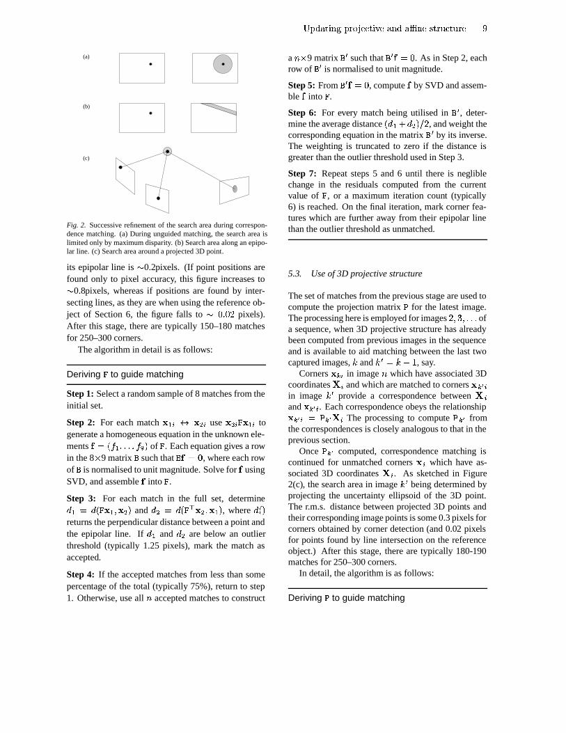
Fig. 2. Successive refinement of the search area during correspon-dence matching. (a) During unguided matching, the search area islimited only by maximum disparity. (b) Search area along an epipo-lar line. (c) Search area around a projected 3D point.

its epipolar line is � 0.2pixels. (If point positions arefound only to pixel accuracy, this figure increases to� 0.8pixels, whereas if positions are found by inter-secting lines, as they are when using the reference ob-ject of Section 6, the figure falls to � � ´ � D pixels).After this stage, there are typically 150–180 matchesfor 250–300 corners.

The algorithm in detail is as follows:

Deriving � to guide matching

Step 1: Select a random sample of 8 matches from theinitial set.

Step 2: For each match P � £+* P H £ use P H £ � P � £ togenerate a homogeneous equation in the unknown ele-ments , Q�V.-Ñ�Z ´@´@´ -0/,] of � . Each equation gives a rowin the 8 K 9 matrix 1 such that 12, Qäi , where each rowof 1 is normalised to unit magnitude. Solve for , usingSVD, and assemble , into � .

Step 3: For each match in the full set, determine3 � Q 3 V � P � Z&P H ] and3 H Q 3 V � ^�P H Z�P � ] , where

3 V�]returns the perpendicular distance between a point andthe epipolar line. If

3 � and3 H are below an outlier

threshold (typically 1.25 pixels), mark the match asaccepted.

Step 4: If the accepted matches from less than somepercentage of the total (typically 75%), return to step1. Otherwise, use all Ü accepted matches to construct

a Ü�K 9 matrix 1�° such that 1�°4, Q � . As in Step 2, eachrow of 1�° is normalised to unit magnitude.

Step 5: From 1�°4, Q � , compute , by SVD and assem-ble , into � .

Step 6: For every match being utilised in 1)° , deter-mine the average distance V 3 � Á 3 H ]65 D , and weight thecorresponding equation in the matrix 1�° by its inverse.The weighting is truncated to zero if the distance isgreater than the outlier threshold used in Step 3.

Step 7: Repeat steps 5 and 6 until there is negliblechange in the residuals computed from the currentvalue of � , or a maximum iteration count (typically6) is reached. On the final iteration, mark corner fea-tures which are further away from their epipolar linethan the outlier threshold as unmatched.

5.3. Use of 3D projective structure

The set of matches from the previous stage are used tocompute the projection matrix O for the latest image.The processing here is employed for images

D Z J Z ´,´@´ ofa sequence, when 3D projective structure has alreadybeen computed from previous images in the sequenceand is available to aid matching between the last twocaptured images, � and ��° Q � Á \ , say.

Corners P � £ in image Ü which have associated 3Dcoordinates S³£ and which are matched to corners P �87 £in image � ° provide a correspondence between S�£and P9� 7 £ . Each correspondence obeys the relationshipP:� 7 £ Q O � 7 S £ The processing to compute O � 7 fromthe correspondences is closely analogous to that in theprevious section.

Once O � 7 computed, correspondence matching iscontinued for unmatched corners P £ which have as-sociated 3D coordinates S £ . As sketched in Figure2(c), the search area in image ��° being determined byprojecting the uncertainty ellipsoid of the 3D point.The r.m.s. distance between projected 3D points andtheir corresponding image points is some 0.3 pixels forcorners obtained by corner detection (and 0.02 pixelsfor points found by line intersection on the referenceobject.) After this stage, there are typically 180-190matches for 250–300 corners.

In detail, the algorithm is as follows:

Deriving O to guide matching

\ � Beardsley et al.

Step 1: Take a random sample of 6 correspondencesfrom the full set of correspondences.

Step 2: For each correspondence S £ * P:� 7 £ in thesample, use the relationship P � 7 £ Q O � 7 Sô£ to generatetwo homogeneous equations in the unknown elementsof O � 7 . (Each correspondence gives three linear homo-geneous equations in the unknown elements of O � 7 andin the unknown homogeneous scale factor; eliminatingthe scale factor then leaves two linear homogeneousequations in the unknown elements ; of O � 7 ). Thesetwo homogeneous equations contribute two rows to a12 K 12 matrix < such that <=; QÀi where each row of< is normalised to unit magnitude. Solve for ; usingSVD and assemble ; into O � 7 .Step 3: For every correspondence in the full set, useO � 7 to project the uncertainty ellipsoid of S £ onto theimage plane, and if P °£ lies within the 95% confidencelimit (see (Zhang & Faugeras 1992)) mark the corre-spondence as accepted.

Step 4: If the percentage of accepted correspondencesin the full set is less than a threshold (typically 75%),return to step 1. Otherwise, use all Ü accepted corre-spondences to construct a

D Ü�K 12 matrix < ° such that<6°>; Q � . As in step 2, each row of <�° is normalised tounit magnitude.

Step 5: From <p°4; Q �, compute ; by SVD and as-

semble ; into O � 7 .Step 6: For every correspondence being utilised inO � 7 , determine the image plane distance � P�� 7 £ Z O � 7 S £ ],� ,and weight the two associated equations in the matrix<6° by its inverse. The weighting is truncated to zero ifP:� 7 £ lies outside the confidence region used in Step 3.

Step 7: Repeat steps 5 and 6 until there is negliblechange in the residuals computed from the currentvalue of O � 7 , or a maximum iteration count (typically6) is reached. On the final iteration, corners whichlie outside their associated projected confidence regionare judged to be incorrect matches, and are marked asunmatched.

5.4. Non-linear refinement of � and O .

The linear estimate of the fundamental matrix provessufficient for processing arising in the course ofan image sequence when � is being used only toguide correspondence matching. For frame initial-isation however it is worth the computational ex-pense of refining the estimate using non-linear op-timisation methods: we used the Powell method(Press et al. 1988). The error measure minimised toobtain � is the sum of the squares of the perpendicu-lar distances of each matched point from its epipolarline (Faugeras et al. 1992)

? Q Ù@BA6CED.FHGJI £ ù � 3=K VYP ù Z � P £ ] H Á 3�K VYP £ Z � ^ P ù ] H �

thus minimising an image plane distance rather thanan algebraic error as in the linear computation. Theimprovement obtained in the average corner-epipolarline distance is typically small, about 0.01 pixels, butthis may result in a movement of many tens of pixelsin the position of the epipoles obtained from � .

The non-linear optimisation also serves a sec-ond purpose: unlike linear processing it permitsenforcement of the constraint that L o�t�M V � ]WQ D(Luong et al. 1993), by making the third row of � a lin-ear combination of the first two rows (Faugeras 1992).

Turning to O , because of its use in computing andupdating the 3D structure, the highest accuracy esti-mate is required and therefore non-linear refinement isalways used. The error measure minimised is the sumof the squares of the image distances between cornerson the image plane and the projection OTS of the 3Dstructure,

? Q Ù N V$P�Z OTS ] H ´6. Results for projective SFM

The primary questions addressed in the experimentalwork are:B How does the quality of recovered structure in a

projective system with uncalibrated cameras com-pare with that from a Euclidean system whichutilises full and accurate camera calibration and es-timates of camera motion?B The approximate camera calibration and motion in-formation used to set up a Quasi-Euclidean coor-dinate frame, Section 3.3, determines the amount

kml nporq_sutpvIl=w�xzy�{,|�q_su}Ñ{ ozt=n³or�Itp{��&q�w_�=|�q_�pw�{ \z\

Fig. 3. The first and last images from a sequence of fifteen images of the reference object.

Fig. 4. Structure of the reference object in a Quasi-Euclidean coordinate frame (connectivity has been added to the point structure for illustra-tion). Although Euclidean relationships such as perpendicularity are not preserved exactly in a Quasi-Euclidean frame, it is evident that theyare approximately true. The right-hand figure is viewed with one of its planes edge-on to show coplanarity in the recovered structure.

of projective distortion between Quasi-Euclideanstructure and true Euclidean structure. How ap-proximate can the camera calibration and motionbe while still producing a “reasonable” Quasi-Euclidean frame?B How does the quality of structure compare in aQuasi-Euclidean frame and a frame with a largeprojective skew?Experiments have been carried out in two types of

environment. The first uses a camera mounted on arobot arm viewing a reference object made of two per-pendicular Tsai calibration grids, and the second usesa camera mounted on a mobile vehicle moving alonga corridor.

The first environment allows us to make quantita-tive assessments of the recovered structure, and wedo so in two ways: first, by measuring projective in-variants directly from the recovered structure, and sec-ondly by transforming to a strictly Euclidean coordi-nate frame by using the known Euclidean structureof the reference object and measuring Euclidean in-variants. The reference object provides a commonreference coordinate frame, allowing proper compar-ison between the quality of the projective structurewith that obtained from conventional Euclidean algo-

rithms. For the second environment, results are pre-sented in the Quasi-Euclidean frame allowing qualita-tive assessment.

6.1. Reference object in the Quasi-Euclidean frame

In these experiments the camera was moved in a hori-zontal circular arc while fixating on the reference ob-ject some 80cm away. The first and last images froma sequence of 15 are shown in Figure 3: the transla-tion and rotation angle between each image are about2cm and 2 ã respectively. To obtain the “best feasible”structure for the reference object, point positions onthe grid are determined not from the corner detector,but by intersecting lines. Figure 4 shows the structureof the reference object recovered in a Quasi-Euclideanframe. Although Euclidean relationships such as per-pendicularity are not preserved, it is evident that theviolation is small.

The cross-ratio is a projective invariant, and can bemeasured directly from the recovered structure. Fourequally spaced collinear points have a cross-ratio of4/3. Thirty-two such cross-ratios are computed foreach image of a sequence, and the results plotted inFigure 5. The measured cross-ratio improves with

\ D Beardsley et al.

0 1 2 3 4 5 6 7 8 9

Image number

1.3380

1.3360

1.3340

1.3320

1.3300

1.3280

1.3260

Cross ratio

1.3333

Fig. 5. The mean values and standard deviations determined for the 32 cross ratios computed from the recovered projective structure updatedduring an image sequence. The expected ratio of 4/3 is shown as a solid line.

Table 1. A comparison with expected geometric values of results obtained using the present projective algorithm, the DROID Euclideanalgorithm, and the affine specialisation (discussed in Section 7). For the projective structure the cross-ratio measurement was made beforetransformation to the Euclidean frame, and the remaining measures after. For the affine structure, the cross-ratio and ratio measurements weremade before transformation to the Euclidean frame, and the remaining measures after. 128 points were used to compute the transformation tothe Euclidean frame. The point error is the average distance between a transformed point and the veridical Euclidean point, in the Euclideanframe. Coplanarity is a mean value for the two faces of the reference object.

Point in Measure Expected Projective Affine DROIDSequence value

After 2 Point error (cm) 0.0 0.2 0.3 0.3images Collinearity 0.0 0.003 0.005 0.006

Coplanarity 0.0 0.004 0.006 0.007Cross-ratio 4/3 1.332 O 0.006 1.333 O 0.003 1.332 O 0.005Distance ratio 1.0 0.999 O 0.012 1.002 O 0.009 1.000 O 0.013

After 20 Point error (cm) 0.0 0.1 0.2 0.2images Collinearity 0.0 0.002 0.002 0.004

Coplanarity 0.0 0.002 0.003 0.004Cross-ratio 4/3 1.333 O 0.002 1.333 O 0.001 1.333 O 0.002Distance ratio 1.0 1.000 O 0.004 1.000 O 0.006 0.999 O 0.007

the sequential update, and converges to the predictedvalue.

Because the reference grid has known structure,it is possible to transform the recovered structure toa strictly Euclidean coordinate frame. The transfor-mation can be determined using the coordinates offive or more points in the Quasi-Euclidean and Eu-clidean frames (Semple & Kneebone 1952) (we em-ploy all 128 points on the reference object in a least-squares computation), where direct physical measure-ment on the reference object provides the Euclideancoordinates.

Comparison between the expected and measuredvalues in columns 3 and 4 of Table 1 provides an over-all assessment of the quality of the recovered projec-tive structure, by showing cross-ratios computed be-

fore transformation to the Euclidean coordinate frameand other measurements like collinearity and copla-narity made after the transformation to ensure that allsuch measurements are in a single reference coordi-nate frame. The collinearity measure P Q VRQ Hù ÁQ H� ] ��S H 5TQ £ and the coplanarity measure â QUQV�W5TVRQ H£ ÁQ Hù ] �6S H were obtained by using SVD to obtain the prin-cipal axes

Ð Z û Z � together with the variance Q £ , Q ù , Q �of point positions along each axis. A straight line isthus expected to have P Q �

and a plane to haveâ Q � . Note that all measures converge as more im-ages are considered.

Column 6 of Table 1 also provides a comparisonwith a local implementation of the DROID system(Harris 1987; Harris & Pike 1987) which computesEuclidean structure directly, requiring, of course, ex-

kml nporq_sutpvIl=w�xzy�{,|�q_su}Ñ{ ozt=n³or�Itp{��&q�w_�=|�q_�pw�{ \ J(a) (b) (c)

Fig. 6. (a) The large white blocks mark two example corners. (b) Uncertainty ellipsoids for the recovered 3D points, projected to ellipseson the image plane, after one update in the sequential update scheme. (c) The ellipses after four updates. The ellipses have shrunk rapidlyas the uncertainty in the 3D points is reduced by successive observations, and the major and minor axes are about 6 pixels and about 1 pixel(approximately 0.4X and 0.1 X ), respectively.

(a) (b)

Fig. 7. (a) Structure of the reference object in a coordinate frame with a large projective skew — coplanarity and collinearity are preserved asexpected, but the structure is skewed along one plane, and the angle between the two planes is less than

%8Y X (connectivity has been added tothe point structure for illustration). (b) Plan view of the computed structure viewed edge-on along the planes of the reference object (lower) andshowing the computed camera positions (upper), in the frame with large projective skew. Compare with the plan view after transformation tothe Euclidean frame in Figure 8.

(b)(a)

Fig. 8. (a) Plan view of the reference object viewed edge-on (lower) and the arc of successive camera positions in a circle (upper) after trans-formation to a Euclidean frame. Note the perpendicularity of the planes of the reference object. (b) View from behind the arc of camerapositions.

act camera calibration and approximate camera mo-tion. Evidently there is no significant difference be-tween the quality of our projective algorithm and theDROID Euclidean algorithm, though we note againthat no camera calibration is required in the projectivecase.

As we discussed in Section 3.4, varying the approx-imate values of camera intrinsic parameters and cam-era rotation used to set up the Quasi-Euclidean frameproduces different amounts of projective skew. To testfor the effects of skew, values for the camera calibra-

tion parameters used in setting up the Quasi-Euclideanframe were varied up to 20% from their true values,and the camera rotation was approximated by settingthe rotation to zero. It was found that this level of vari-ation had no effect on the assessments listed in Table1.

Finally, Figure 6 shows some examples of the un-certainty ellipsoids for recovered 3D points, projectedonto the image plane. Each example is computed bytaking the uncertainty ellipsoid for a 3D point at imageÐ

and projecting it onto imageÐ Á \ , finding the ellipse

\ M Beardsley et al.

which has a 95% likelihood of containing the newobservation of the 3D point(Zhang & Faugeras 1992);such ellipses are used to define search areas for corre-spondence matching (Section 5.3).

6.2. Reference object in a non Quasi-Euclideanframe

Section 6.1 dealt with structure recovered in a Quasi-Euclidean frame. Here, structure and camera positionare computed in a coordinate frame which has a largeprojective skew away from being Euclidean. An ex-ample transformation ± Þ between such a frame and aEuclidean frame was given earlier in Section 3.4. Fig-ure 7 shows structure recovered for the reference ob-ject in such a frame. The transformation away from thetrue Euclidean form is partly evident in the projectiveskew of the grid itself, but is most evident from the factthat the plan view shows the planes of the grid in a Zwhich is directed away from the camera positions c.f.Figure 3 where it is apparent that the Z is towards thecamera physically. Figure 8 shows the structure andcamera positions from Figure 7 after transformation toa Euclidean frame.

6.3. Comparison of structure in the Quasi-Euclideanand non Quasi-Euclidean frames

A comparison between measurements on 3D struc-ture in a Quasi-Euclidean frame and in a frame witha large projective skew is given in Table 2, and showsthe superiority of the Quasi-Euclidean frame. Mea-surements are given after 2 images when the structurehas just been initialised, after 3 images when there hasbeen one update, and after 10 images. There is a fur-ther partition of results according to the level of local-isation accuracy in the image points utilised to com-pute the structure. Three levels of localisation accu-racy were explored. First, using line intersection tocompute point positions, an accuracy of 0.02 pixelsis obtained. Secondly, the positions are rounded tothe nearest 0.1 pixels and the structure recomputed,and finally rounded to the nearest integer pixel and thestructure again recomputed.

One trend evident in the results is that in all mea-sures the accuracy is better in the Quasi-Euclideanframe. A second trend is that the difference in ac-curacy between the Quasi-Euclidean and non Quasi-

Euclidean diminishes as information from more im-ages is integrated, although when using the referenceobject no new structure is being introduced betweenframes. A third observation is that as the localisationaccuracy is reduced to nearest pixel, the non Quasi-Euclidean reconstruction cannot be continued: the ini-tial structure is so erroneous that the computed per-spective projection matrix results in predicted imagepositions differing from their veridical positions bygreater than 10 pixels.

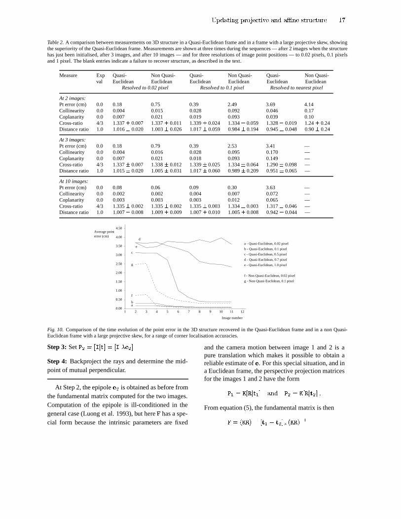
Figure 10 gives a more detailed graphical compari-son of of the point error (the first measure in Table 2)in the structure recovered in a Quasi-Euclidean frameand in a non Quasi-Euclidean frame with a large pro-jective skew for a range of corner localisation accu-racies. The recovered structure is transformed to theEuclidean coordinate frame of the reference object,and the average distance between transformed pointsand the veridical positions of points on the referenceobject measured. The point errors are plotted overa sequences of 11 images. Notice that at a locali-sation error of 1 pixel no improvement in the Quasi-Euclidean structure is discernible over this time scale.At the finer localisations, the Quasi-Euclidean alwaysout-performs the non Quasi-Euclidean reconstruction.

6.4. Structure from motion of a mobile vehicle

Figures 9(a and b) show the first and last images of a12 image sequence taken by a camera mounted on amobile vehicle which translated forward along a cor-ridor while turning to the left. The maximum depthof the scene is about 7m. Corners were obtained usingthe sub-pixel corner detector discussed earlier. Figures9(c and d) show the structure recovered in a Quasi-Euclidean frame from two different vantage points.Notice that Euclidean relationships such as perpendic-ularity of the side wall and floor are approximatelycorrect, and the quality of the reconstruction remainshigh even at the most distant points.

6.5. Summary of results

The questions posed at the start of this section can nowbe related to the experimental results.B There is effectively no difference in the quality of

the structure recovered by the Quasi-Euclidean pro-jective algorithm and the strictly Euclidean DROID

kml nporq_sutpvIl=w�xzy�{,|�q_su}Ñ{ ozt=n³or�Itp{��&q�w_�=|�q_�pw�{ \ Äsystem, although the latter has the stronger con-straints and utilises accurate camera calibration.Table 1 shows that both at initialisation and at alater stage in the sequence, all the evaluation mea-sures are similar. Note the accuracy of recoveredstructure: the structure is accurate to within 1mm,after transformation to a Euclidean frame, for anobject at a distance of 80cm.B The initialisation of a suitable Quasi-Euclideanframe is not sensitive to the particular approxima-tion of camera calibration and motion (Section 6.1).B The Quasi-Euclidean frame produces superiorstructure to a coordinate frame which has a largeprojective skew away from Euclidean, as shown inFigure 10. This is a consequence of the methodused to initialise 3D points. The method has therequirement that the coordinate frame is Quasi-Euclidean (whereas there are approaches whichavoid this as discussed in Section 3.3), but offersthe most straightforward and computationally effi-cient way of handling error in the image measure-ments.B Sequential update of the structure over time usingan iterated EKF provides a way of integrating manyobservations of a point in a computationally effi-cient way. There is no guarantee of optimality orconvergence with an EKF but empirically the qual-ity of the recovered structure improves under thesequential update as demonstrated in Figure 5, andthe structure has been found to be stable providedthe number of gross mismatched corners is reducedusing the outlier detection methods described inSection 5.

7. Affine Structure from Motion

The previous sections of the paper, particularly Sec-tion 3, have dealt with the computation of projectivestructure. Here we specialise our approach to recoveraffine structure. The objective of the affine structurefrom motion algorithm is to use correspondences be-tween corners P in a sequence of images to recover thestructure S of the scene, modulo an affine transforma-tion. That is, if the Euclidean structure of the scene isS º , the recovered structure is

S Q�±2[ Sôº

where S Q VYaRZ�c»Z2emZ@\�]_^ , S º Q VYa º Z_c º Z2e º Z@\�]�^ ,and ± [ is an affine transformation which is undeter-mined but the same for all points:± [ Q ·]\ hi�^ \ ¹with \ a non-singular JLK³J matrix and h a 3-vector.

An affine coordinate frame differs from a projectivecoordinate frame because the plane at infinity ^ Ò hasbeen identified (Semple & Kneebone 1952).

Our approach is a variation on a result of Moonset al. (1993) who showed that affine structure can beobtained from a perspective camera with fixed intrin-sic parameters undergoing pure translational motion.Unlike (Moons et al. 1993) which is based on a smallfixed number of image points, we use all available im-age points to set up the affine frame. Note that affinestructure is being obtained from perspective images,and there is no need to assume affine imaging con-ditions; that is, there is no need to assume weak orpara-perspective cameras. (Sequential computation ofaffine structure under affine imaging conditions is de-scribed in (McLauchlan et al. 1994).)

7.1. Setting an affine coordinate frame.

This section describes initialisation of an affine coor-dinate frame. Unlike the projective case where thereare several significant modifications to obtain a Quasi-Euclidean frame, only one modification to the basicprocessing is required to obtain a Quasi-Euclideanaffine coordinate frame. To maintain similarity withthe projective case, we will call this Step 0 in the fol-lowing listing:

Setting an Affine Frame

Step 0 (optional): If the coordinate frame is tobe Quasi-Euclidean, normalize the image coordinatesP�Ç V$�=Æ@] ¦ � P in both images.

Step 1: Set O � Q��¶µp� iT� .Step 2: Determine the fundamental matrix � . Use it todetermine the epipole ¿ H in the second image.

\ Ô Beardsley et al.

(b)(a)

(d)(c)

Fig. 9. (a) and (b) First and last images taken by a camera mounted on a mobile vehicle as it moves forward and turns left. (c) and (d). The3D structure viewed in the Quasi-Euclidean frame from two viewpoints. (The overlaid image texture is created by mapping between Delaunaytriangulations of the 2D image corners.)

kml nporq_sutpvIl=w�xzy�{,|�q_su}Ñ{ ozt=n³or�Itp{��&q�w_�=|�q_�pw�{ \ óTable 2. A comparison between measurements on 3D structure in a Quasi-Euclidean frame and in a frame with a large projective skew, showingthe superiority of the Quasi-Euclidean frame. Measurements are shown at three times during the sequences — after 2 images when the structurehas just been initialised, after 3 images, and after 10 images — and for three resolutions of image point positions — to 0.02 pixels, 0.1 pixelsand 1 pixel. The blank entries indicate a failure to recover structure, as described in the text.

Measure Exp Quasi- Non Quasi- Quasi- Non Quasi- Quasi- Non Quasi-val Euclidean Euclidean Euclidean Euclidean Euclidean Euclidean

Resolved to 0.02 pixel Resolved to 0.1 pixel Resolved to nearest pixel

At 2 images:Pt error (cm) 0.0 0.18 0.75 0.39 2.49 3.69 4.14Collinearity 0.0 0.004 0.015 0.028 0.092 0.046 0.17Coplanarity 0.0 0.007 0.021 0.019 0.093 0.039 0.10Cross-ratio 4/3 1.337 _ 0.007 1.337 _ 0.011 1.339 _ 0.024 1.334 _ 0.059 1.328 _ 0.019 1.24 _ 0.24Distance ratio 1.0 1.016 _ 0.020 1.003 _ 0.026 1.017 _ 0.059 0.984 _ 0.194 0.945 _ 0.048 0.90 _ 0.24

At 3 images:Pt error (cm) 0.0 0.18 0.79 0.39 2.53 3.41 —Collinearity 0.0 0.004 0.016 0.028 0.095 0.170 —Coplanarity 0.0 0.007 0.021 0.018 0.093 0.149 —Cross-ratio 4/3 1.337 _ 0.007 1.338 _ 0.012 1.339 _ 0.025 1.334 _ 0.064 1.290 _ 0.098 —Distance ratio 1.0 1.015 _ 0.020 1.005 _ 0.031 1.017 _ 0.060 0.989 _ 0.209 0.951 _ 0.065 —

At 10 images:Pt error (cm) 0.0 0.08 0.06 0.09 0.30 3.63 —Collinearity 0.0 0.002 0.002 0.004 0.007 0.072 —Coplanarity 0.0 0.003 0.003 0.003 0.012 0.065 —Cross-ratio 4/3 1.335 _ 0.002 1.335 _ 0.002 1.335 _ 0.003 1.334 _ 0.003 1.317 _ 0.046 —Distance ratio 1.0 1.007 _ 0.008 1.009 _ 0.009 1.007 _ 0.010 1.005 _ 0.008 0.942 _ 0.044 —

Average pointerror (cm)

Image number

a - Quasi-Euclidean, 0.02 pixel

b - Quasi-Euclidean, 0.1 pixel

c - Quasi-Euclidean, 0.5 pixel

d - Quasi-Euclidean, 0.7 pixel

e - Quasi-Euclidean, 1.0 pixel

f - Non Quasi-Euclidean, 0.02 pixel

g - Non Quasi-Euclidean, 0.1 pixel

0.00

0.50

1.00

1.50

2.00

2.50

3.00

3.50

4.00

4.50

1 2 3 4 5 6 7 8 9 10 11 12

b

f

g

e

d

c

a

Fig. 10. Comparison of the time evolution of the point error in the 3D structure recovered in the Quasi-Euclidean frame and in a non Quasi-Euclidean frame with a large projective skew, for a range of corner localisation accuracies.

Step 3: Set O H Q��uµp� h@� Q¾�uµp� × ¿ H �Step 4: Backproject the rays and determine the mid-point of mutual perpendicular.

At Step 2, the epipole ¿ H is obtained as before fromthe fundamental matrix computed for the two images.Computation of the epipole is ill-conditioned in thegeneral case (Luong et al. 1993), but here � has a spe-cial form because the intrinsic parameters are fixed

and the camera motion between image 1 and 2 is apure translation which makes it possible to obtain areliable estimate of ¿ . For this special situation, and ina Euclidean frame, the perspective projection matricesfor the images 1 and 2 have the formO ��QÅ� � ��� hr�_� ozt=n O H QÅ��� ��� h H � ´From equation (5), the fundamental matrix is then� Q�V$���p] ¦ ^ � h � ��h H ��¨�VY�6�p] ¦ �

\ � Beardsley et al.

0.9850

0.9950

1.0050

1.0150

0 2 4 6 8 10 12 14 16 18 20 22 24

Ratio

1.0

Image number

Fig. 11. Ratios computed from recovered affine structure against image number. The points and error bars show the mean and standard deviationfor a fixed number (thirty-two) of ratio values computed at each image. The horizontal line shows the expected value of unity for the ratio.

rear boxesviewed edge-on

"dan" box

"RM" box

right obstacleleft obstacle right obstacle

left obstaclewhite box

(a)(b)

Fig. 12. Two images from a sequence with structure recovered in a Quasi-Euclidean affine frame. (a) Plan view of recovered structure. (b)View from the right and to the rear of the obstacles.

which is of the form � Q \ ^ � \ where � is skew-symmetric. It follows that � is skew symmetric. Fur-ther, since � is unaffected by a projective transforma-tion of the world frame, the same argument holds inany coordinate frame, not just a Euclidean one. Be-cause � is skew symmetric, it has only three distincthomogeneous elements or two degrees of freedom, asopposed to seven degrees of freedom in the generalcase. This substantial reduction in the number of un-knowns makes the computation more efficient and bet-

ter conditioned. The skew form also means that therank 2 condition on � is imposed automatically dur-ing the linear computation. (As we saw earlier, thisis not possible for the general form, where the rank 2condition must be imposed in a non-linear step.)

Note that at Step 2, unlike the projective case, wedid not need to compute � H . This is because at Step3, when O ��Q �uµp� ip� and when the camera has fixedintrinsic parameters and undergoes a pure translation,it is standard to set O H Q �uµp� × ¿ H � . This choice sets

kml nporq_sutpvIl=w�xzy�{,|�q_su}Ñ{ ozt=n³or�Itp{��&q�w_�=|�q_�pw�{ \ íthe plane at infinity to ^ Ò Q�V � Z � Z � Z@\]&^ , the conven-tional value for an affine frame. This may be verifiedusing Lemma 2 in Appendix C.

7.2. Updating the affine coordinate frame.

The previous section addressed the initialisation anaffine coordinate frame. Here we describe a methodfor transforming an existing arbitrary projective coor-dinate frame into an affine frame, using a pure trans-lational motion of the camera. This can be used toupdate an existing affine frame which has “drifted”slightly over time. Strictly this should be unneces-sary because the coordinate frame is fixed once it hasbeen set up but in practice the need to recompute theframe can arise for two reasons. First, as structure isupdated the plane at infinity may drift due to error.Secondly, the motion made in order to determine theplane at infinity might not be pure translation, and theerror which arises in an individual measurement canbe overcome by making repeated measurements.

Updating an Affine Frame

Step 1. At the current step û determine O�ù for the cam-era position in the established coordinate frame.

Step 2. Keeping the intrinsic coordinates fixed, makethe camera undergo pure translation. Determine O ù6` �for the new camera position in the established coordi-nate frame.

Step 3. Transform the coordinate frame so that O ùtakes the canonical form O °ù Q �uµp� ip� . Apply the trans-formation to Opù6` � to obtain O=°ù6` � QÀ� � ù6` � �@h Æ � .Step 4. Decompose � ù6` � into � × µ Á h Æ «)^ usingLemma 2, where × is a scale factor, and « a vector.The plane at infinity is now ^ Ò QÀVY«)^mZ@\�] .Step 5. Transform the whole coordinate frame oncemore so that the plane at infinity takes its conventionalform of ^ Ò Q¾V � Z � Z � Z,\�] .

Step 4 exploits Lemma 2 which, with its proof,is given in Appendix C. Also in Appendix C is themethod for decomposing �ba `9c so that « can be found.

7.3. Results for affine SFM

Experiments similar to those for projective structurein Section 6 were carried out. Quasi-Euclidean affinestructure is computed for two image sequences, one ofthe reference object and the other of an indoor scene.Assessment is by (i) measurement of affine invariantsdirectly from the recovered structure and (ii) measure-ments on the structure after transformation to a Eu-clidean frame.

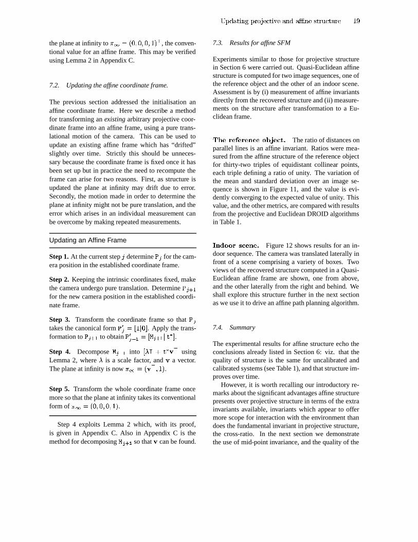
d ü)¿fer¿ , ¿=e¿�gVhz¿ji Â�k ¿�hzhWl The ratio of distances onparallel lines is an affine invariant. Ratios were mea-sured from the affine structure of the reference objectfor thirty-two triples of equidistant collinear points,each triple defining a ratio of unity. The variation ofthe mean and standard deviation over an image se-quence is shown in Figure 11, and the value is evi-dently converging to the expected value of unity. Thisvalue, and the other metrics, are compared with resultsfrom the projective and Euclidean DROID algorithmsin Table 1.

m g9nVibioeqp�hz¿�gÿ¿ol Figure 12 shows results for an in-door sequence. The camera was translated laterally infront of a scene comprising a variety of boxes. Twoviews of the recovered structure computed in a Quasi-Euclidean affine frame are shown, one from above,and the other laterally from the right and behind. Weshall explore this structure further in the next sectionas we use it to drive an affine path planning algorithm.

7.4. Summary

The experimental results for affine structure echo theconclusions already listed in Section 6: viz. that thequality of structure is the same for uncalibrated andcalibrated systems (see Table 1), and that structure im-proves over time.

However, it is worth recalling our introductory re-marks about the significant advantages affine structurepresents over projective structure in terms of the extrainvariants available, invariants which appear to offermore scope for interaction with the environment thandoes the fundamental invariant in projective structure,the cross-ratio. In the next section we demonstratethe use of mid-point invariance, and the quality of the

D �Beardsley et al.

affine reconstruction, by using the structure to drivepath-planning for navigation.

8. Navigation in Affine Space

The affine SFM scheme provides the basis for naviga-tion through an unknown environment of unmodelledobstacles. We investigate to what extent affine struc-ture can be used for a task which is traditionally car-ried out with Euclidean information. The experimentalsetup is a camera mounted on a robot arm moving ina horizontal plane and rotating around a vertical axis.The objective is to reach a target position specified inthe robot’s coordinate frame. The area in between thestart and target positions is unknown and may containobstacles as illustrated in Figure 13.

8.1. Structure recovery

Processing begins with initialisation of a Quasi-Euclidean affine coordinate frame as described in Sec-tion 7, and sequential update of affine scene structurewith initialisation of newly appearing points using themethods from Section 4. Remaining stages involve in-cremental acquisition of free space regions, path plan-ning through the free space, and finally control of therobot.

8.2. Computing free space

The computation of free space and path planning iscarried out in 2D on the ground plane. This simpli-fication is sufficient for navigation of a robot arm ormobile vehicle which is constrained to execute motionin the plane and is well modelled by a vertical cylinder.The recovered structure and camera positions are pro-jected onto the ground plane using a method describedin Section 8.4.

Computation of free space is complicated by thefact that the recovered structure consists solely ofpoints so there is no representation of continuous sur-faces, and thus no notion of objects or the free spacebetween objects. We begin with the assumptions firstthat recovered points lie on surfaces and so are notisolated in space, and second that points cover eachsurface with sufficient density to make the surface de-tectable — that is, there are no large homogeneous

regions on surfaces (the latter assumption is definedmore rigorously below). A simple occlusion test isthen used to detect free space as sketched in Fig-ure 14a. Consider first the 3D information prior toprojection to the ground plane. If a scene point â isvisible continuously as the camera moves from r � tor H (this may be over several images rather than be-tween consecutive images), then there is no occludingsurface in the triangle defined by r � âsr H . The pro-jection of this free space triangle to the ground planedefines a free space triangle on the 2D map.

A necessary modification of this test, shown in Fig-ure 14b, is that the projection of r � âsr H onto theground plane is accepted as free space only if noother projected 3D point t lies within that triangle.The modification is required for a number of reasons.Firstly, point t might arise from a low object u inthe foreground while â is a point which is visibleabove and to the rear of u , in which case the pro-jected r � âsr H clearly should not be accepted as freespace because it overlays u ; this situation relates tothe assumption made at the start of the paragraph thatu must generate points in “sufficient density” to in-dicate its presence and prevent the acceptance of freespace triangles which overlay it. Secondly, the modi-fication deals with the case of concave objects whereâ arises from a point within a concavity and t is apoint on the convex hull of the projected object i.e.we prevent the marking of the inside of the concav-ity as free space on the projected map. Thirdly andfinally, the modification is conservative, and preventsthe acceptance of free space triangles when there is amismatched or badly localised point present.

The complete free space map is the union of all ac-cepted triangles — thus the more corners there are inthe images, the more detailed will be the computedfree space. An alternative approach to free spacecomputation involving the use of points to constructa polyhedral approximation to an object is describedin (Faugeras 1993). The identification of obstacles di-rectly from range data for map building in a navigationsystem is described in (Langer et al. 1994).

8.3. Path planning

Path planning involves the determination of a routeto the target, passing only through areas which havebeen confirmed to be free space. Use of the mid-line, an affine construct, through an area of free space

kml nporq_sutpvIl=w�xzy�{,|�q_su}Ñ{ ozt=n³or�Itp{��&q�w_�=|�q_�pw�{ D \Target

Obstacles

Background

Camera onrobot arm

Fig. 13. The experimental setup. A camera carried by a robot arm manouevres to a target through an environment of unmodelled obstacles.

C1 C2

(a) (b)

C1 C2

Point P Point P

Point Q

Fig. 14. The camera moves from v�w to vyx observing continuously a point z in the scene. (a) The projection of v�wJz{v�x onto the ground planedoes not contain any other projected points so it is marked as free space. (b) The projection of v w z{v x is unacceptable as free space becauseof the presence of | ; however v�w6|}v�x is accepted as free space. See discussion in the text.

is fundamental to the adopted approach. The expla-nation below is given with reference to Figure 15which shows actual free space maps computed dur-ing the processing (further examples are given in(Beardsley et al. 1994)). Figure 15(a) is a schematicplan view of the environment, where there is no directroute from the initial camera position to the target be-cause of the presence of obstacles u \zZ u D Z u J . Figure15(b) shows the free space map computed as describedin Section 8.2 after several small lateral camera mo-tions have been executed, and affine structure com-puted. The free space extends forward from the cam-era, is truncated at u \ and u D , but a central lobe ex-tends through the gap between the obstacles. Once theinitial map has been obtained, a check is made to seewhether there is an unobstructed route of free spaceto the target. If not, a search is made for the lobe offree space whose midline is most closely aligned withthe direction to the target. This involves measurementof angle which is not an affine invariant but, as we

are working in a Quasi-Euclidean frame, approximatemeasurements of angle are available. The trajectoryfrom the current camera position to a point on the mid-line, and then along the midline, is checked to see howfar the camera can proceed. Checking the trajectoryinvolves knowledge of the camera dimensions, whichare stored as Euclidean measurements. The issue oftransforming between the affine frame and a Euclideanframe so that Euclidean dimensions can be utilised isdiscussed in the next section.

Figure 15(c) shows the free space after the camerahas moved through the gap between the obstacles u �and u H . A lateral camera motion has been carried outat the new position, and affine structure computed forthe newly visible parts of the scene. Newly detectedfree space has been used to incrementally enlarge thefree space map, the new area being truncated by obsta-cle u F to the left and terminating at the obstacle to therear of the scene. The route to the target is rechecked

DzDBeardsley et al.

250 500 750

-1250

-1000

-750

-500

-250

250

500

750

1000

1250

250 500 750

-1250

-1000

-750

-500

-250

250

500

750

1000

1250

250 500 750

-1250

-1000

-750

-500

-250

250

500

750

1000

1250

y (mm)

Target

Camera-750

-500

-250

0

250

500

750

750500250

Rear of scene

x (mm)

x (mm) x (mm)

y (mm)

y (mm)y (mm)

initial camera

"lobe" of free space

new cameraposition

newly detected lobeof free space

trajectory of camera

projected pointsfrom obstacles

rear of scene

Obstacle O3

x (mm)

O2

O3

projected points from

O1

(b)(a)

(c) (d)

O1 O2Obstacles

targettarget

position

Fig. 15. (a) Schematic plan view of the experimental layout showing the initial camera position, obstacles ~ #8� ~ ��� ~ ! , the target position, andthe rear of the scene. The semi-circle indicates the workspace of the robot arm. (b) Free space (black) computed after the initial camera motions,extending forward from the camera which is at the lower part of the figure. The left and right-hand sides of the free space are terminated atabout ���j� #�Y8Y where there are obstacles but the central “lobe” of free space extends through the gap between the obstacles to about ��� !�*8Y .(c) Updated free space map after the robot has proceeded through the gap and rechecked the target. (d) Projection of 3D structure and camerapositions (connected line) onto the ground plane. The full trajectory of the camera from the initial to the target position is shown.

kml nporq_sutpvIl=w�xzy�{,|�q_su}Ñ{ ozt=n³or�Itp{��&q�w_�=|�q_�pw�{ D Jand the process in the previous paragraph repeated, re-sulting in a new camera motion.

Figure 15(d) shows the computed affine structure(isolated points) and the camera motion (connectedline).

8.4. Computation of transformations

Two transformations which arise in the navigation pro-cessing are the 3D-2D transformation for the pro-jection of 3D structure to the ground plane in theaffine frame, and a 2D-2D transformation between theground plane in the affine frame and the ground planein the Euclidean robot frame.

�o������� ; e�i k ¿�h�h��RiogNh�iLh,üÿ¿���e0i��9gVn ;ÿ¢R� g)¿�l Pro-jection of 3D point positions to the ground plane in theaffine coordinate frame requires knowledge of the ver-tical direction. This is in fact readily available sincethe camera is mounted such that its [ -axis is vertical,and the axes of the camera and the affine coordinateframes are aligned at initialisation (Section 7.1). Thusthe vertical direction is aligned with the c -axis of theaffine frame, and a 3D point S Q¾V$abZ�c»Z2emZ@\] projectssimply to S Þ Q¾VYaRZ2emZ@\�] on the ground plane.

��������� hHe � gVp , ioe0� � h��Ei�g  ¿�h ý ¿6¿�g ��� g)¿ � gVne0i  i=h , e � �è¿�pWl A full 3D transformation betweenthe affine coordinate frame and the robot coordinateframe is not needed, since motions are in a horizontalplane and information about height above the groundplane is not relevant. Thus it suffices to obtain a 2Dtransformation for the ground plane. The transforma-tion can be found given the coordinates of four or morenon-collinear points on the ground plane in the affineframe, and their corresponding position on the groundplane in the robot coordinate frame. Computationof the transformation utilises optical centre positionscomputed in the affine frame in the normal course ofthe SFM processing, with the corresponding positionsin the robot frame being provided by the robot, and nospecial calibration is necessary. All computed camerapositions are utilised in a least-squares linear compu-tation.

The primary use of the transformation between theaffine and robot frames is to enable motions in theaffine frame to be mapped to Euclidean commands forthe robot. This could potentially be avoided because

the robot could be controlled by visual servoing alone.For example, with no calibration the robot could bedriven to rotate until a certain point (for instance anaffine invariant such as a centroid) was at the middle ofthe image. This has not been addressed since the focusof the work so far has been on the computation of 3Dstructure. In addition, the transformation has two fur-ther uses: first, the dimensions of the robot assemblywhich carries the camera are specified as Euclideanmeasurements; and, secondly, the target position forthe robot motion is specified as a Euclidean positionin the robot coordinate frame.

9. Conclusion

This paper has demonstrated the initialisation of pro-jective and affine structure from image sequences,with an accuracy similar to a system using calibratedcameras. The work has been implemented in a systemwhich has been extensively tested on real images, withautomatic and reliable correspondence matching, andthe use of robust techniques to detect outliers. Therecovery of projective and affine structure is increas-ingly well-understood, but its use in practice raises in-teresting problems about what can be achieved whenEuclidean measurements are not available. Here affinestructure has been applied to path planning.

The possibility of utilising a constraint such astranslational motion (Moons et al. 1993) to obtainaffine structure underlies a spectrum of possibili-ties for investigation, ranging from fully calibratedstereo heads through to cameras of unknown intrin-sic parameters and motion. The precision of theconstraints and the stage at which they are intro-duced interplay to determine the type of the recov-ered structure and motion — projective, affine, or Eu-clidean — and its accuracy. This echoes the ideaof stratification introduced by Koenderink and vanDoorn (Koenderink & VanDoorn 1991).

Here we have concentrated on the uncalibratedend of this spectrum. We have provided a mecha-nism — via the Quasi-Euclidean frame — for incor-porating poor or partial camera calibration. Thereare many remaining questions concerning the con-straints required, and the stage at which they are intro-duced, when specialising structure. For example, thereare various ways to specialise projective structure toaffine; by translation as demonstrated, or by identify-ing distant points (Faugeras 1992). Further specialisa-

D M Beardsley et al.

tion to scaled Euclidean structure is possible by cam-era self-calibration (Faugeras et al. 1992), or by otherconstraints on lengths and angles (Mohr et al. 1993a).The interaction and application of such constraints of-fers numerous possibilities for extension of the ideaspresented here.

Finally, the work has highlighted a number of is-sues which proved to be of key importance in exper-imental terms, although their importance was not al-ways immediately evident in the mathematical theory.

� ¿=gVp��Yh��$«b�Yh)� h�i����Ep�� � h�hü)¿�p&l The computationof the fundamental matrix � and the perspective pro-jection matrix O is affected by mismatched corners. Itis crucial to remove mismatches since, even if they ap-pear to be having only a small effect in individual com-putations, they cause a cumulative degradation overtime as the structure is updated. As described in Sec-tion 5, we employ a three-stage process in which mis-matches are identified as outliers in the computationof � and O . Empirically, the computation of � is moreresilient to outliers than the computation of O , so � isfound first.f�� �è¿=e � ��i�h��Ei�g�l The conditioning of the compu-tation of � becomes poorer as the distance between thecamera optical centres gets smaller. We have utilisedlarge motions between images of 1-3cm.

� �Enÿ¿ � � gV� ¢ ¿ ¢ ¿�gVpWl Use of a wide angle lens (afield of view of about

Ä � ã ) leads to better camera lo-calisation because rays from the optical centre to thescene have good divergence; it also makes it easier tofix each new camera position in the ongoing coordi-nate frame because many points remain in view be-tween images.

� ioe ý � e0n���i�h��Riog�l Simple forward motion pro-duces poor structure because rays from the camera toa 3D point change angle slowly (relative to the ef-fect of a lateral motion) resulting in large error in thecomputed point position. To avoid this, forward mo-tion paths could be “dithered” with lateral movements(stereo would be of obvious benefit in this role). In-stead, a 3D point is not initialised from its first two ob-servations if the angle between the backprojected raysis below a threshold (

D ã ), but the observations are ac-cumulated until the angle exceeds the threshold. Onlythen is initialisation is carried out, using all the back-

projected rays in a generalisation of the 2-ray scheme:the 3D point is found as that which minimises the sumof the square distances between the 3D point to eachbackprojected ray.f e0�$h��Eh �p¢ p��:e ,�� hÑ¿=p&l The problem of critical sur-faces in structure from motion is well-known (see forexample (Maybank 1993)). A special case of the gen-eral form of a critical surface arises in our environmentwhen a planar surface fills (or nearly fills) the field ofview. This suggests a need to explicitly test for criti-cal surfaces and switch to more qualitative processingwhen detected.

� io��i���¿=gÿ¿�io�Vp hWibioe0n9�Rg � h�¿�pWl The arbitrary ho-mogeneous component in a homogeneous vector istypically chosen as unity — e.g., an image cornerVYXÈZ�[p] is represented as VYXÈZ�[ Z@\�] . Increased stabilityis achieved if the third component is chosen to be ofthe same order of magnitude as X and [ (Section 3.3).Similar remarks apply to points in 3D.f ioe0g)¿=e�� � h�hü9�Rg9�9l The cross-correlation used tomeasure strength of match between corners is initiallyon raw image intensity to avoid unnecessary computa-tion. However, if the matching between a pair of im-ages appears to be failing at any stage (which is testedby examining whether the ratio of number of matchesto total number of corners is below a threshold), thenthe matching is restarted with cross-correlation on nor-malised intensity. The normalisation is effectivelydone by dividing the pixel patch at a corner by itsmean intensity. The initiation of normalisation oc-curs for two reasons in practice: (i) changing illumina-tion is an obvious effect which will cause matching onraw image intensity to fail; and (ii) the automatic gaincontrol of the camera may adjust the grey-level inten-sity across the whole image in response to some eventsuch as a bright area appearing on the image periph-ery; again, this will prevent matching on raw intensity.

Acknowledgements

This work was supported by Grant GR/H77668 fromthe UK EPSRC, by Esprit Grant BRA 6448 ‘VIVA’from the EC, and by and the Newton Institute, Cam-bridge, under SERC Grant GR/G59981. The authorshave profited from discussions with Richard Hartley,

kml nporq_sutpvIl=w�xzy�{,|�q_su}Ñ{ ozt=n³or�Itp{��&q�w_�=|�q_�pw�{ D ÄJitendra Malik, Joe Mundy, and with colleagues inthe Robotics Research Group, particularly AndrewBlake, Mike Brady, Phil McLauchlan, Ian Reid, LarryShapiro, Phil Torr and Bill Triggs. Adrian Cox pro-vided considerable advice on operating the Adeptrobot arm.

Appendix A: Lemma 1

LEMMA 1 Given two cameras with distinct opticalcentres and fundamental matrix � , and the perspectiveprojection matrix for the first camera in the canonicalform O � QÀ�¶µp� iT� , then O H has the general formO H Q¾� � HªÁ ¿ H� ^ ��Ã�¿ H �where ¿ H , the epipole in the second image, satisfies� ^�¿ H Q � ; � H is a particular solution of � QÀ� ¿ H � ¨ � H ;and  and à are an arbitrary 3-vector and scalar re-spectively.

Proof:This proof follows closely Hartley’s proof of the

uniqueness of decompositions of the fundamental ma-trix (Hartley 1992). Suppose O H Q¬� � H ��h H � and O °H Q� � °H �2h °H � are two possible O H matrices consistent with � .Since O ��Q��uµp� ip� , the optical centre of the first camerahas coordinates f ��Q¾V � Z � Z � Z,\�]�^ . The epipole in thesecond image is the projection of the optical centre.Applying O H and Op°H we haveO H f �äQ h H Q × ¿ HO °H f �äQ h °H Q × ° ¿ H ´Thus h H Q�h °H QÅ¿ H up to a scale factor.

Next from equation (5) for the fundamental matrixdefined from projection matrices, we have:� Q�� ¿ H � ¨ � H QÀ� ¿ H � ¨ � °H ´It follows that � ¿ H � ¨ V$� H ��� °H ]mQ � and so � H ��� °H Q¿ H� ^ .

Thus, allowing for the overall scale factor, there arefive homogeneous parameters or four DOF in O H . Val-ues for � H and ¿ H are obtained by decomposing � asdescribed next.

A.1 Decomposing �The first step is to obtain ¿ H from the equation � ^ ¿ H Q�

. If � Q V , ��Z , H Z , F ] , where , £ are the columns of � ,then , £ ´ ¿ H Q � . Thus the epipole can be computed as¿ H Q , � K�, H .

The second step is to compute a particular � H . Note,that there is not a unique decomposition since (fromthe proof of the lemma) if � is a particular solution,then so is � Á ¿ H n�^ where n is an arbitrary 3-vector.The equation � Q�� ¿ H �&¨�� H , (with both ¿ H and � of rank2 and known) is a linear equation for � H with fewerequations than unknowns because of the rank 2 ma-trices. A particular solution can be found by standardmethods (Press et al. 1988).

Appendix B: Transformation between Euclideanand Quasi-Euclidean frames

We develop theory to quantify the residual projectiveskew in the Quasi-Euclidean frame.

Consider two cameras with the same intrinsic pa-rameters � , separated by a rotation � and translationh . Then a Euclidean coordinate frame is obtained bysetting the perspective projection matrices toO º � Q ���¶µp� iT��QÀ� ��� ip�O ºH Q � ����� × ö¿ H �where × Q¡ ��6�6h=  , ö¿ H is the epipole in image 2 nor-malised so that the sum of its squared components isunity, and it has been made explicit that the last col-umn of O H is a multiple of ö¿ H . (For the purposes ofexplanation, we will keep � explicit here.)

Now consider a projective coordinate frame set upwith O �äQ � � Æ � iT�O H Q � � Æ � Ƽ � ò ö¿ H �where ò is the scale of the reconstruction.

Wen now show that the transformation S Q± ¦ � S º between the Euclidean and projective framesis ±IQ²·£¢¤ � ¦ � � Æ i« ^ \ ¹ (13)

where « ^ Q ò ¦ � ö¿ ^H VY� Æ � Ƽ �§�6�6� ¦ � � Æ ] ´

D�ÔBeardsley et al.

Consider two cameras with the same intrinsic pa-rameters � , separated by a rotation � and translationh . Then Euclidean structure, S º , is obtained from theperspective projection matrices:O º � Q¥���¶µp� iT��QÀ� ��� iT�O ºH Q¥��� ������6h���QÀ� �6��������6h@��Q�� �6��� × ö¿ H � (14)

where × Q¥ ����6�6h=  , ö¿ H is the epipole in image 2 nor-malised so that the sum of its squared components isunity, and it has been made explicit that the last col-umn of O H is a multiple of ö¿ H .

If instead the projection matrices are chosen asO � Q � � Æ � ip�O H Q � � Æ � Ƽ � ò ö¿ H � (15)

then the recovered structure, S , is related to S º , bythe projective transformation S Qű ¦ � S º , where±LQ²·¦¢¤ � ¦ � � Æ i«)^ \ ¹ (16)

with « ^ Q ò ¦ � ö¿ ^H V$� Æ � Ƽ ���6��� ¦ � � Æ ] ´ (17)

Proof: Under the transformation S Q�± ¦ � SÛº , equa-tion (7) shows the projection matrices transform asO º � ±ÓQ O � (18)O ºH ±ÓQ O H ´ (19)± can be written as±LQ · \ Âh�^ 3 ¹where \ is a 3 K 3 matrix,  and h are 3-vectors, and

3a scalar. From equation (18) it follows that \ QÅ� ¦ � � Æand  QÅi i.e.±LQ · � ¦ � � Æ ihÑ^ 3 ¹ Zand from equation (19)� ���6� ¦ � � Æ ÁU× ö¿ H h ^ � 3 × ¿ H � QÀ� � Æ � Ƽ � ò ¿ H � ´ (20)

Pre-multiplying the left J»K�J matrices of equation (20)by ö¿T^H gives

h ^ Q × ¦ � ö¿ ^H VY� Æ � Ƽ �����6� ¦ � � Æ ]�Z

and the final column gives3 Q ò 5 × . An overall scal-

ing gives the form of ± in equations (16) and (17).

Appendix C: Lemma 2

LEMMA 2 Given two camera matrices O ��Qñ�uµT� ip�and O H Q � ��� h Æ � for identical cameras related bya pure translation, matrix � can be decomposed as�NQ × µ Á h Æ « ^ where × is a scale factor, and ^ Ò QVY«)^mZ@\�]�^ is the equation of the plane at infinity.

Proof:The proof is based on the approach given

in (Mundy 1993). The cameras have identical intrinsicparameters, and their positions differ only by a puretranslation. Thus, assuming image coordinates havebeen normalised according to equation (8), the projec-tion matrices for a Euclidean frame areO º � Q � ���r�§�6h�2�O ºH Q � ���r�§�6h H �

The Euclidean structure S º and projective struc-ture S are related by S º Q�± S , where±IQ²·�\ p«)^ \ ¹ ´The projection matrices in the projective frame areO � Q O º � ±O H Q O ºH ± ´ (21)

The O � equality gives× �¶µp� iT��Q���� \ ��h�2« ^ � p��§hr�_�where × is an arbitrary scale factor. Hence,

páQ¥h�� \ Q × µ Á �6h � « ^ ´From the O H equality (equation (21)), if follows thath Æ Q ��� h�»��h H �� Q × µ Á h Æ « ^ ´

This completes the first part of the proof. It onlyremains to demonstrate that ^ Ò Q V$«)^�Z,\�]&^ is the

kml nporq_sutpvIl=w�xzy�{,|�q_su}Ñ{ ozt=n³or�Itp{��&q�w_�=|�q_�pw�{ D óequation of the plane at infinity. The point transforma-tion matrix is S Qá± ¦ � S º , hence the plane transfor-mation matrix is ±�^ (Semple & Kneebone 1952). Thecoordinates of the plane at infinity in the Euclideanframe are ^ ºÒ Q²V � Z � Z � Z,\�]�^ . Therefore the coordi-nates in the projective frame are

^ Ò Q¥± ^ ^ ºÒQ©V$« ^ Z,\�] ^C.1 Solving for × and «Given � and h Æ we now describe how to obtain × and« from �G� × µ�Q�h Æ « ^ ´

This is an eigen-vector problem: the matrix h Æ «)^is rank one, so × must be a repeated eigen-value of � .Call this eigen-value × � , associated with eigen-vectors¿2§ and ¿�¨ , and the remaining eigen-value × H associ-ated with eigen-vector ¿y© . ThenVY�Í� × �rµ�]&¿ © Q©V ×�H � × �,]�¿ © (22)Q©VYh Æ « ^ ]�¿ © Q h Æ V$«�ª,¿ © ]Hence ¿�© is parallel to h Æ . For the other eigen-vectors(Ð QU«�Z_Î )VY�Í� × �rµ�]&¿ £ QÅh Æ « ^ ¿ £ QÅh Æ VY«¬ª@¿ £ ]¡Qji ´

Hence ¿�§�Z�¿2¨ are both perpendicular to « , and there-fore «§Q ò ¿ § K ¿ ¨ (23)

where ò is an unknown scale. This scale ò is deter-mined from equation (22) as follows:«�ª,¿ © Q V ×�H � × �,]H @¿ ©   Hh Æ ª@¿2©and, taking the scalar product with « in equation (23),ò Q V ×�H � × �,]H @¿ ©   HVYh Æ ª@¿T] © � ¿ © Z�¿ § Z�¿ ¨ � ´

References

Armstrong, M., Zisserman, A., and Beardsley, P.A. 1994. Euclideanreconstruction from uncalibrated images. To appear in Proc. 5thBritish Machine Vision Conference, York, UK.

Ayache, N. 1991. Artificial vision for mobile robots. MIT Press,Cambridge MA.

Bar-Shalom, Y. and Fortmann, T.E. 1988. Tracking and Data Asso-ciation. Academic Press, San Diego CA.

Beardsley, P.A., Zisserman, A.P., and Murray, D.W. 1994. Navi-gation using affine structure and motion. In Proc. 3rd EuropeanConference on Computer Vision, Stockholm, pp. 85–96. Springer-Verlag, Berlin.

Deriche, R., Zhang, Z., Luong, Q.T., and Faugeras, O. 1994. Robustrecovery of the epipolar geometry for an uncalibrated stereo rig.In Proc. 3rd European Conference on Computer Vision, Stock-holm, pp. 567–576. Springer-Verlag, Berlin.

Faugeras, O.D. 1992. What can be seen in three dimensions withan uncalibrated stereo rig? In Proc. 2nd European Conference onComputer Vision, Santa Margherita Ligure, Italy, pp. 563–578.Springer-Verlag, Berlin.

Faugeras, O.D. 1993. Three-dimensional computer vision: a geo-metric viewpoint. MIT Press, Cambridge MA.

Faugeras, O.D., Luong, Q.T., and Maybank, S.J. 1992. Cameraself-calibration: theory and experiments. In Proc. 2nd EuropeanConference on Computer Vision, Santa Margherita Ligure, Italy,pp. 321–334. Springer-Verlag, Berlin.

Fischler, M.A. and Bolles, R.C. 1981. Random sample consensus:a paradigm for model fitting with application to image analysisand automated cartography. Commun. Assoc. Comp. Mach.,24:381–95.

Harris, C.G. 1987. Determination of ego-motion from matchedpoints. In Proc. 3rd Alvey Vision Conference, Cambridge, UK,pp. 189–192.

Harris, C.G. and Pike, J.M. 1987. 3D positional integration fromimage sequences. In Proc. 3rd Alvey Vision Conference, Cam-bridge, UK, pp. 233–236.

Harris, C.G. and Stephens, M. 1988. A combined corner and edgedetector. In Proc. 4th Alvey Vision Conference, Manchester, UK,pp. 147–151.

Hartley, R. 1992. Invariants of points seen in multiple images.Technical Report, The General Electric Corporate Research andDevelopment Laboratory, Schenectady, NY, USA. To appear inIEEE Transactions on PAMI.

Hartley, R., Gupta, R., and Chang, T. 1992. Stereo from uncali-brated cameras. Proc. IEEE Conference on Computer Vision andPattern Recognition. IEEE Computer Society Press, WashingtonDC.

Hartley, R.I. 1993. Euclidean reconstruction from uncalibratedviews. In Proc. 2nd European-US Workshop on Invariance,Azores, pp. 187–202.

Hollinghurst, N. and Cipolla, R., 1993. Uncalibrated Stereo Hand-Eye Coordination. In Proc. 4th British Machine Vision Confer-ence, Guilford, UK, pp. 389–398. BMVA Press, 1993.

Koenderink, J.J. and van Doorn, A.J. 1991. Affine structure frommotion. J. Opt. Soc. Am. A, 8(2): 377–385.

Langer, D., Rosenblatt, J.K., and Hebert, M. 1994. An integratedsystem for autonomous off-road navigation. In Proc. IEEE Int.Conf. on Robotics and Automation, San Diego CA, pp. 414–419.IEEE Computer Society Press, Los Alamitos CA.

Latombe, J.C. 1991. Robot Motion Planning. Kluwer AcademicPublishers.

DT�Beardsley et al.

Luong, Q.T., Deriche, R., Faugeras, O.D. and Papadopoulo, T.1993. On determining the fundamental matrix. Technical Re-port No.1894, INRIA, Sophia-Antipolis, France.

Luong Q.T. and Vieville, T. 1994. Canonic representations forthe geometries of multiple projective views. In Proc. 3rd Eu-ropean Conference on Computer Vision, Stockholm, pp 589–597.Springer-Verlag, Berlin.

Maybank, S.J. 1993. Theory of Reconstruction from Image Motion.Springer-Verlag, Berlin.

McLauchlan, P.F., Reid, I.D., and Murray, D.W. 1994. Recursiveaffine structure and motion from image sequences. In Proc. 3rdEuropean Conference on Computer Vision, Stockholm, pp. 217–224. Springer-Verlag, Berlin.

Mohr, R., Boufama, B., and Brand, P. 1993a. Accurate projectivereconstruction. In Proc. 2nd European-US Workshop on Invari-ance, Azores, pp. 203–228.

Mohr, R., Veillon, F., and Quan, L. 1993b. Relative 3D reconstruc-tion using multiple uncalibrated images. Proc. IEEE Conferenceon Computer Vision and Pattern Recognition, pp. 543–548. IEEEComputer Society Press, Washington DC.

Moons, T., van Gool, L., van Diest, M., and Oosterlinck, A.1993. Affine structure from perspective image pairs under rel-ative translations between object and camera. Technical ReportKUL/ESAT/M12/9306, Departement Elektrotechniek, KatholiekeUniversiteit Leuven, Belgium.

Mundy, J.L. 1993. Repeated structures: Image correspondence con-straints and ambiguity of 3D reconstruction. In Proc. 2nd Work-shop on Applications of Invariance in Computer Vision, Azores,pp. 51–63.

Mundy, J.L. and Zisserman, A.P. 1992. Geometric Invariance inComputer Vision. MIT Press, Cambridge MA.

Press, W., Flannery, B., Teukolsky, S., and Vetterling, W. 1988.Numerical Recipes in C. Cambridge University Press.

Reid, I. D. and Murray, D. W. 1993. Tracking foveated corner clus-ters using affine structure. In Proc. 4th International Conferenceon Computer Vision, Berlin, pp. 76–83. IEEE Computer SocietyPress, Los Alamitos, CA.

Semple, J.G. and Kneebone, G.T. 1952. Algebraic Projective Ge-ometry. Oxford University Press.

Szeliski, R. and Kang, S.B. 1993. Recovering 3D shape and motionfrom image streams using non-linear least squares. Technical Re-port 93/3, Digital Equipment Corporation Research Laboratories.

Torr, P.H.S., Beardsley, P.A., and Murray, D.W. 1994. Robust vi-sion. To appear in Proc. 5th British Machine Vision Conference,York, UK.

Torr, P.H.S. and Murray, D.W. 1997. The Development and Com-parison of Robust Methods for Estimating the Fundamental Ma-trix International Journal of Computer Vision. 24 (1997) 271–300

Zhang, Z. and Faugeras, O.D. 1992. 3D Dynamic Scene Analysis.Springer-Verlag, Berlin.