14
Series & Parallel AC Circuits Analysis ET 242 Circuit Analysis II Electrical and Telecommunication Engineering Technology Professor Jang
| Date post: | 02-Jan-2016 |
| Category: |
Documents |
| Upload: | abigayle-miller |
| View: | 236 times |
| Download: | 1 times |

Series & Parallel AC Circuits Analysis
ET 242 Circuit Analysis II
Electrical and Telecommunication Engineering Technology
Professor Jang

AcknowledgementAcknowledgement
I want to express my gratitude to Prentice Hall giving me the permission to use instructor’s material for developing this module. I would like to thank the Department of Electrical and Telecommunications Engineering Technology of NYCCT for giving me support to commence and complete this module. I hope this module is helpful to enhance our students’ academic performance.

OUTLINESOUTLINES
Introduction to Series - Parallel
ac Circuits Analysis
Analysis of Ladder Circuits
Reduction of series parallel Circuits to Series Circuits
ET 242 Circuit Analysis II – Series-Parallel Circuits Analysis Boylestad 2
Key Words: ac Circuit Analysis, Series Parallel Circuit, Ladder Circuit
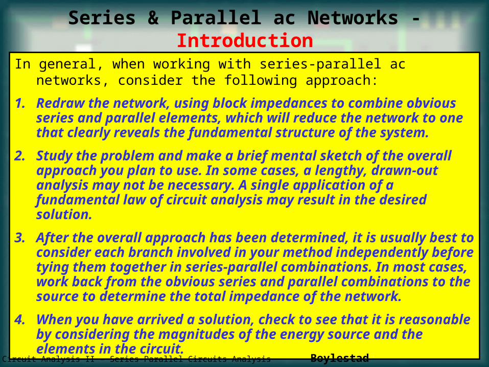
Series & Parallel ac Networks - Introduction
In general, when working with series-parallel ac networks, consider the following approach:
1. Redraw the network, using block impedances to combine obvious series and parallel elements, which will reduce the network to one that clearly reveals the fundamental structure of the system.
2. Study the problem and make a brief mental sketch of the overall approach you plan to use. In some cases, a lengthy, drawn-out analysis may not be necessary. A single application of a fundamental law of circuit analysis may result in the desired solution.
3. After the overall approach has been determined, it is usually best to consider each branch involved in your method independently before tying them together in series-parallel combinations. In most cases, work back from the obvious series and parallel combinations to the source to determine the total impedance of the network.
4. When you have arrived a solution, check to see that it is reasonable by considering the magnitudes of the energy source and the elements in the circuit.
ET 242 Circuit Analysis II – Series-Parallel Circuits Analysis Boylestad 3

ET 242 Circuit Analysis II – Series-Parallel Circuits Analysis Boylestad 12
Ex. 16-1 For the network in Fig. 16.1: a. Calculate ZT. b. Determine Is. c. Calculate VR and VC. d. Find IC.
e. Compute the power delivered. f. Find Fp of the network.
a. As suggested in the introduction, the network has been redrawn with block impedances, as shown in Fig. 16.2. Impedance Z1 is simply the resistor R of 1Ω, and Z2 is the parallel combination of XC and XL.
Figure 16.1 Example 16.1.
54.8008.661
906901
06
1
06
32
)903)(902(
)90)(90(//
0
21
2
1
21
jZZZand
j
jj
jXjX
XXZZZ
RZ
withZZZ
bydefinedisimpedancetotalThe
T
LC
LCLC
TFigure 16.2 Network in Fig. 16.1 after assigning the block impedances.

80.5419.74A
80.546.08Ω
0120
Z
EIb
Ts.
9.46118.44V)90)(6Ω80.54(19.74AZIV
80.5419.74V)0)(1Ω80.54(19.74AZIV
:lawsOhm'ofnapplicatiodirectaby
foundbecanVandVthatfindweFig.16.2.toReferringc
2sC
1sR
CR.
leading0.164cos80.54cosθFf
W389.67(1Ω1(19.74A)RIPe
80.5459.22A902Ω
9.46118.44V
Z
VI
:lawsOhm'usingfound
alsobecanIcurrenttheknown,isVthatNowd
p
22sdel
C
CC
CC
.
.
.
ET 242 Circuit Analysis II – Series-Parallel Circuits Analysis Boylestad 5
6.8780A53.135
60400
j43
60400
j4Ω4(3Ωj8Ω8(
)30)(50A90(8Ω
ZZ
IZI
yieldsruledividercurrenttheUsing
908Ωj8ΩjXZ
53.135Ωj4Ω3ΩjXRZ
havewe16.4,Fig.inascircuittheRedrawinga
12
2
C2
L1
.
ET 242 Circuit Analysis II – Parallel ac circuits analysis Boylestad 6
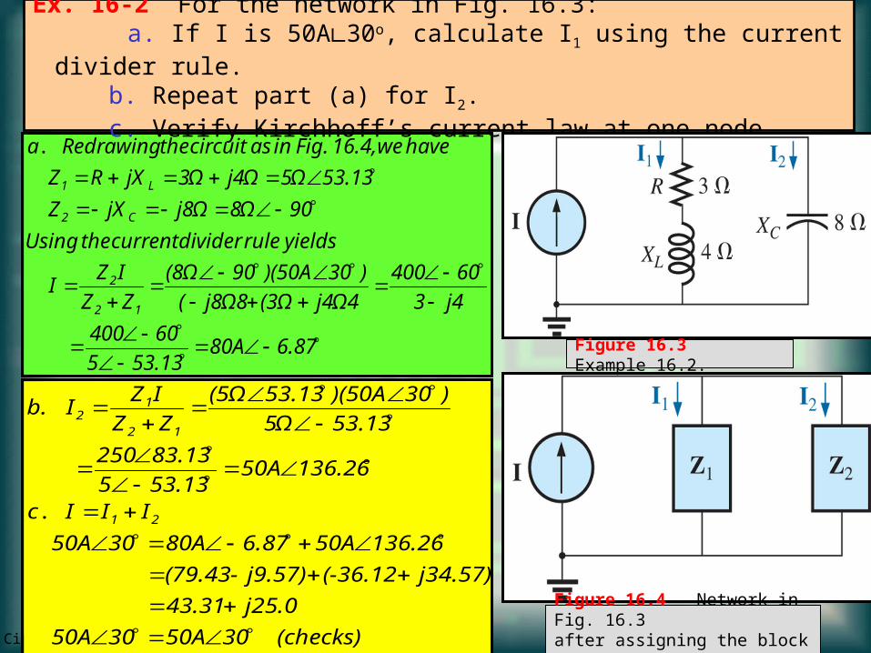
Ex. 16-2 For the network in Fig. 16.3: a. If I is 50A∟30o, calculate I1 using the current divider rule.
b. Repeat part (a) for I2.c. Verify Kirchhoff’s current law at one node.
Figure 16.3 Example 16.2.
Figure 16.4 Network in Fig. 16.3 after assigning the block impedances.(checks)3050A3050A
j25.043.31
j34.57)(-36.12j9.57)-(79.43
136.2650A6.8780A3050A
IIIc
136.2650A53.135
83.13250
53.135Ω
)30)(50A53.13(5Ω
ZZ
IZIb.
21
12
12
.

ET 242 Circuit Analysis II – Parallel ac circuits analysis Boylestad 2
Ex. 16-3 For the network in Fig. 16.5: a. Calculate the voltage VC using the voltage divider rule.
b. Calculate the current Is.
Figure 16.5 Example 16.3.
Figure 16.6 Network in Fig. 16.5 after assigning the block impedances.
62.246.1838.6713
70240
125
)2020)(9012(
9088
901212
055
,6.16.
.
21
2
3
2
1
VV
j
V
ZZ
EZV
jZ
jZ
Z
withFigin
shownasredrawnisnetworkThea
C
41.051.23Aj0.810.93I
j1.54)(0.07j2.35)(0.86
87.381.54A702.5AIII
and
87.381.54A67.3813Ω
2020V
ZZ
EI
702.5A53.138Ω
2020V
Z
EIb.
s
21s
212
31

26.5622.36A26.564.472Ω
0100V
Z
EIand
26.564.472Ω10.3011.18
16.2650Ω
j211
16.2650Ω
Ω)jΩ(Ω)jΩ(
).Ω)(.Ω(
ZZ
ZZZ
36.8710Ωj6Ω8ΩjXRZ
53.135Ωj4Ω3ΩjXRZ
obtainweFig.16.8,inascircuittheRedrawinga
Ts
21
21T
C22
L11
6843
87361013535
.
Ex. 16-4 For Fig. 16.7: a. Calculate the current Is.
b. Find the voltage Vab.
Figure 16.7 Example 16.4.
Figure 16.8 Network in Fig. 16.7 after assigning the block impedances.
73.74100Vj9628j48)(36j48)(64
53.1360V36.8780VVVVor
0VVV
12
21
RRab
RRab
36.8780V)0)(8Ω36.87(10AZIV
53.1360V)0)(3Ω53.13(20AZIV
36.8710A36.8710Ω
0100V
Z
EI
53.1320A53.135Ω
0100V
Z
EI
law,sOhm'Byb.
22
11
R1R
R1R
22
11
ET 242 Circuit Analysis II – Series-Parallel Circuits Analysis Boylestad 8

Ex. 16-6 For the network in Fig. 16.12: a. Determine the current I.
b. Find the voltage V.
51.4022.626mAj2.052mA1.638mA
4mAj2.052mA5.638mA04mA206mAIT
63.43522.361kΩ
j20kΩ10kΩZ
01.545kΩ
0//6.8kΩ02kΩZ
obtainweFig.16.13,inas
circuittheRedrawing
2
1
111.410.18mA
60.0041023.093
51.4024.057A
10j201011.545
51.4024.057A
j20kΩ10kΩ1.545kΩ
)51.402)(2.626mA0(1.545kΩ
ZZ
IZI
ruledividerCurrent
333
21
T1
:
a. The equivalent current source is their sum or difference (as phasors).
47.973.94V
)63.435)(22.36kΩ111.406(0.176mAIZVb 2.
Figure 16.12 Example 16.6.
Figure 16.8
ET 242 Circuit Analysis II – Series-Parallel Circuits Analysis Boylestad 9

ET 242 Circuit Analysis II – Parallel ac circuits analysis Boylestad 10
Ex. 16-7 For the network in Fig. 16.14: a. Compute I. b. Find I1, I2, and I3 c. Verify KCL by showing that
I = I1 + I2 + I3. d. Find total impedance of the circuit;.
6
10
.
j8
j9-j3Ω8Ω
jXjXRZ
j4Ω3ΩjXRZ
0ΩRZ
wherenetworkparallel
strictlyarevealsFig.16.15in
ascircuittheRedrawinga
CL32
L22
11
2
1
43.18316.01.03.0
06.008.016.012.01.0
87.361.013.532.01.087.3610
1
13.535
11.0
68
1
43
1
10
1
111
tan
321321
SSjS
SjSSjSS
SSS
S
jj
ZZZYYYY
isceadmittotalThe
T
435.182.63
)435.18326.0)(0200(
:
A
VEYI
IcurrentThe
T
Figure 16.14 Example 16.7.
Figure 16.15 Network in Fig. 16.14 following the assignment of the subscripted impedances.

ET 242 Circuit Analysis II – Parallel ac circuits analysis Boylestad 11
87.362087.3610
0200
13.534013.535
0200
020010
0200
,.
33
22
11
AV
Z
EI
AV
Z
EI
AV
Z
EI
branchesparallelacrosssametheisvoltagetheSinceb
44.1817.3435.18316.0
11.
)(20602060
)1216()3224()020(
87.362013.53400202060
. 321
SYZd
checksjj
jjj
j
IIIIc
TT
Ex. 16-8 For the network in Fig. 16.18: a. Calculate the total impedance ZT. b. Compute I. c. Find the total power factor. d. Calculate I1 and I2. e. Find the average power delivered to the circuit.
87.3610
4
.
j6Ω8ΩjXRZ
37.87-11.40j7Ω9ΩjXRZ
0ΩRZ
haveewFig.16.19,inascircuittheRedrawinga
L33
C22
11
Figure 16.18 Example 16.8.
Figure 16.19 Network in Fig. 16.14 following the assignment of the subscripted impedances.
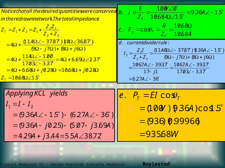
ET 242 Circuit Analysis II – Series-Parallel Circuits Analysis Boylestad 12
5.168.10
28.068.1028.068.64
37.269.6437.303.17
00.11144
)68()79(
)87.3610)(87.374.11(4
:.
32
32121
T
T
Z
jj
jj
ZZ
ZZZZZZ
impedancetotalThenetworkredrawnthein
conservedwerequantitiesdesiredtheallthatNotice
684.10
68.10cos.
5.136.95.1684.10
0100.
TTp
T
Z
RFc
AV
Z
EIb
3627.6
37.303.17
37.397.106
117
37.397.106
)68()79(
)5.136.9)(87.3740.11(
:.
32
22
A
A
j
A
jj
A
ZZ
IZI
ruledividercurrentd
72.385.544.329.4
)69.307.5()25.036.9(
)3627.6()5.136.9(21
AjA
AjjA
AA
III
yieldsKCLApplying
W
AV
EIPe TT
68.935
)99966.0)(936(
5.1cos)36.9)(100(
cos.

Ladder networks were discussed in some detail in Chapter 7. This section will simply apply the first method described in Section 7.6 to the general sinusoidal ac ladder network in Fig. 16.22. The current I6 is desired.
ET 242 Circuit Analysis II – Parallel ac circuits analysis Boylestad 13
Ladder Networks
T
'T21T
''T43
'T
65''T
31
TTT
ZEIThen
//ZZZZwith
//ZZZZand
ZZZ
16.23.Fig.indefinedareIandI
currentsandZandZZceIndependan
''' ,,
Figure 16.22 Ladder network.
Figure 16.23 Defining an approach to the analysis of ladder networks.


