Motion Control and Industrial Controllers World class competitors are moving heavily into CIM (computer integrated manufacturing), JIT (just in time) and TQC (total quality control). Each of these require more flexibility in the manufacturing process, a flexibility often achieved through motion control.
Need for Motion Control
The transfer line and the assembly line have had a powerful impact in automating our factories, especially during the middle decades of the 20th century. Their primary goal was reduction of labor content with the financial justification labeled as economy of scale. With labor now less than 10 percent of the cost of manufactured goods in this country and total employment in manufacturing less than 15 percent of the labor force, something more is needed. What is required is motion control and automation that is more flexible and offers other advantages besides mass production. Some desirable advantages include: producing parts near the point of use, producing any of a family of parts based on customer needs, keeping finished inventory minimized, and responding quickly to customer requests.
These economy of scope installations typically cost 40 to 50 percent more than their predecessors because of the high degree of flexibility that must be built in - often through motion control. The earlier transfer and assembly lines used limit switches to turn motors ON and OFF at fixed positions for the single part for which it was designed. When a family of parts was involved, the dimensions needed to be changed each time a different part came along. This has lead to the use of continuous feedback rather than limit switches; and servo motors and controllers rather than induction motors with ON/OFF contactors. An indication of this trend can be seen in the fact that the motion control segment of the numerical machine control market is growing at about 30 percent compared to the total market which is growing at only 20 percent.
Due to these changing needs, the people responsible for designing and manufacturing new automation equipment are being forced to deal with servos and are facing a myriad of difficult choices and questions. Some of these questions will be discussed. A discussion of a basic servo follows this discussion.
Need a Velocity Loop?
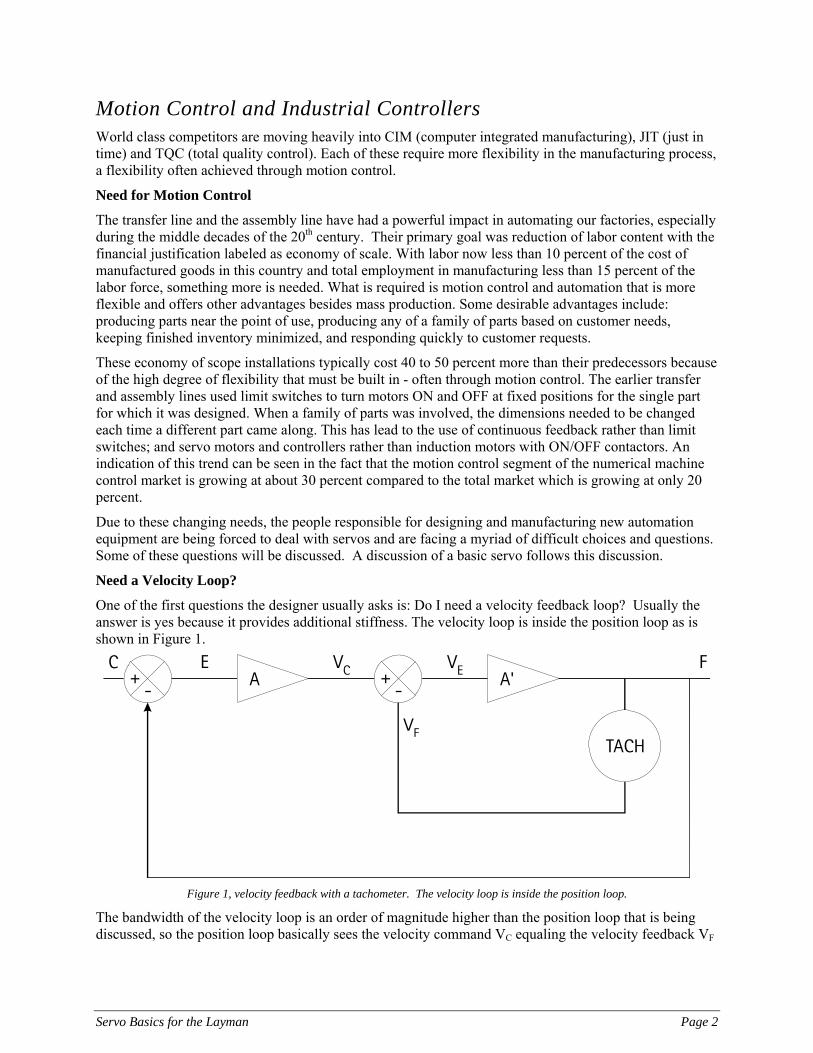
One of the first questions the designer usually asks is: Do I need a velocity feedback loop? Usually the answer is yes because it provides additional stiffness. The velocity loop is inside the position loop as is shown in Figure 1.
Figure 1, velocity feedback with a tachometer. The velocity loop is inside the position loop.
The bandwidth of the velocity loop is an order of magnitude higher than the position loop that is being discussed, so the position loop basically sees the velocity command VC equaling the velocity feedback VF
Servo Basics for the Layman Page 2
for frequencies within its bandwidth. This is important so that the velocity loop does not change the gain, and thereby the stability of the position loop. When VF is not exactly equal to VC, there is an additional gain factor A' to help with forcing. This is what provides the higher stiffness.
In the real world, a position loop can sit with a constant error because that error is not so large that it can develop enough motor torque to overcome static friction. When the velocity loop is added, this error is multiplied by the additional factor of A' until friction is broken and motion takes place so that VF can once again equal VC. A simple test can be made to show the impact of a velocity loop. If one grabs the shaft of a motor without a velocity loop, he will find that he can turn it and hold it out of position indefinitely. If the velocity loop is activated, he will find that he can initially turn it the same amount, but it will immediately fight his action and turn the shaft back into position. This is stiffness and it results in better accuracy.
Do I Run a Hard Servo or a Soft Servo?
High gain servos have come to be known as hard and low gain servos as soft. The higher the gain (A), the greater the bandwidth (the frequency when A = 1). If one tries to raise the bandwidth too much, the natural frequencies of the machine come into play and eventually instability occurs causing the machine to oscillate indefinitely. In addition, as one increases the bandwidth, the servo tries to force the machine more and more to follow the command. A step input in the command will force the machine to jump.
Over time, a machine could be beat to death by an oversized drive system that is forever jerking it back and forth in response to commands. The practical approach is to vary the gain and test the machine's response to a step in command. That response can be viewed on an oscilloscope for number of overshoots or one can rely on gut feel based on how the machine looks when the step occurs. For heavy industry, 1 IPM/MIL (inches per minute per mil of error) is a typical gain. It is unusual for a piece of industrial machinery to get above 5 IPM/MIL.
What Effect Does Gain Have on Performance?
The higher the gain, the less error (E) required to break friction or maintain velocity. The error required to break friction will affect position accuracy at the end of a move, which makes it a major factor in achieving repeatability. The error to break static friction can be measured with the loop closed by slowly changing the command (C) by its least increment while observing the buildup of the error (E). As noted earlier, a velocity loop will have a major impact on the error required to break friction. This test should be done at several points along the travel since mechanical variations will cause the breakaway friction to change.
Another common problem is null hunt, a phenomenon in which an axis moves back and forth with a square waveform at a low frequency. This is usually caused by the breakaway or static friction being significantly higher than the running friction. Essentially, the error builds up to break friction, but once motion starts the error is more than necessary to maintain the desired velocity so it overshoots the desired position. This continues to repeat in both directions. It can be prevented by lowering the gain, however lowering the gain will also affect accuracy. Lowering the ratio of static to running friction can be achieved with roller bearings or, as is more common now, through the use of a special coating material as one of the bearing surfaces. A static to running ratio of 1.01 or less is achievable in this manner.
Accuracy during motion is a concern in many applications. Cutting metal, routing wood, etching glass, and grinding silicon wafer edges are examples where extreme accuracy during motion is required. A servo with a gain of 1 IPM/MIL will have 0.001" of error when traveling at 1 IPM, 0.01" at 10 IPM and 0.1" at 100 IPM. It follows that the best accuracy can be achieved by keeping velocities low and gain high. This is a good generality, but not always that simple to achieve.
Servo Basics for the Layman Page 3
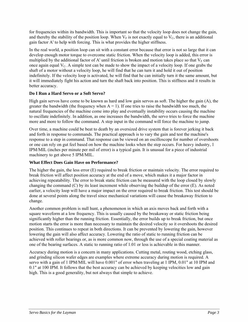
Figure 2, a two-axis move along a 45° slope where both X and Y are commanded at the same velocity.
What Is Required to Maintain Accuracy During Coordinated Motions?
The magnitude of the error really does not matter if the path being followed is a single axis move. The axis will trail the moving command, but will catch up when the endpoint is reached. One could not detect, by observing the cut, that an error ever existed. When two axes are moved simultaneously to generate a sloping straight cut, large errors can develop. Figure 2 shows a two axis move along a 45° slope where both X and Y are being commanded at the same velocity. The gain of the X axis is twice that of the Y axis, so the X axis error (EX) is half that of the Y axis error (EY). The resulting path is offset from the commanded one depending on direction, velocity, gains and angle of slope. If the gains of the two axes in the example were identical, EX and EY would be identical and the machine would lag the moving command, but it would be precisely on the desired path. It would catch up when the command stops at the endpoint. Once the gains are precisely matched, the direction, velocity and angle of slope no longer matter. As long as the commanded path remains on a straight line, the axes will always lag, but precisely on that line. Maintaining accuracy for linear moves becomes an exercise in matching gains. This will require detuning the more responsive axes to match the poorest performing one. Many systems allow gains to be set digitally (and thereby precisely). Often the gain will be a potentiometer or digital register adjustment. This adjustment is made by commanding each axis at the same medium range value and adjusting the potentiometers to achieve equal errors.
Circular moves, where the commanded path is generated by circular interpolation, is another story. Again, the axes gains must be matched or one will be cutting eggs instead of circles. With matched gains, circles will always result, but not necessarily of the commanded size. With low velocities and high circle radii, errors are negligible, however, as the ratio of velocity to circle radius increases, the error in the circle size increases. This raises the question: Will the resultant circle be larger or smaller than the commanded one? (Think about this before reading on.)
There will be servo lag errors, so the machine will lag behind command. As the velocity increases or the radius decreases, will the lagging point move outside the circle or inside? Many people will say that the lagging point moves outside the circle resulting in too large of a circle. This is because they are viewing it like centrifugal force, which it is not. For example, if you hooked a short rubber band with a weight on it to a pencil and drew a circle, the weight would fall farther and farther inside the circle as the rubber band stretched (which is what occurs at higher velocities).
Servo Basics for the Layman Page 4
The amount by which the circle is smaller is very predictable based on velocity, radius and gain, but the equations are more complex than can be covered in this article. There are empirical charts available that relate these factors.
Figure 3, commanding the amount of error with feedforward.
What is Feedforward And Will It Benefit Me?
Most controllers allow use of feedforward. Since the error due to velocity commands is so predictable once the gain is precisely known (and often in digital form in the controller anyway), it is a relatively simple matter to alter the command by the amount of error so that the machine position coincides with the command as is illustrated in figure 3.
If one wants C to equal F, then FF must equal E. Since the commanded velocity and the gain are known in the controller, the error can be computed and added to the command to generate a pseudo command to the servo to cause C and F to be coincident.
Through the proper use of feedforward, it is no longer necessary to precisely match gains, although each gain would still need to be known exactly. Also, for circles, the feedforward would command a pseudo-circle of larger size so that the resultant circle is equal to the one desired.
Contours can be done with feedforward as long as the path can be described with straight lines and circles with the transition points between them tangential. At discontinuous "corners," one must think through what may happen. The two diagrams in figure 4 illustrate what happens at a 90° corner which is executed at velocity.
Servo Basics for the Layman Page 5
Figure 4, an example of what happens at a 90° corner that is executed at velocity.
A normal servo, which lags the command, will round the corner as the second axis command builds up and the lag in the first axis dissipates. With feedforward, since the machine is coincident with the command when the corner is reached and the feedforward for the first axis is removed in a step fashion, the first axis will respond similar to its step response.
What About Servo Update Time?
Control vendors update their servos on a regular time basis. Servo update time is the time interval between the calculations for command (C) minus feedback (F) to give error (E). In other words, it is how often a correction (E) is calculated. Update times vary from microseconds up to 16 ms (milliseconds) for most controllers. Some vendors initially updated servos once per scan with their programmable controller. However, variations in scan time caused severe servo problems, especially when axes needed to be coordinated. Typically the software for closing the servo loop is written in assembly language which is OK since it is invisible to the user. Assembly language is the best to use because it is the most efficient with computer time, especially since it interrupts the computer so often. To conserve computer time, it would seem logical to choose the longest servo update time possible, however, sample data theory would tell one to choose the shortest. In a study of this conducted by myself and Dr. John Bollinger of the University of Wisconsin, the conclusion was that a 10 ms servo update time would be more than adequate for heavy duty industrial machinery. This has proven to be true.
Many vendors are also closing the velocity loop digitally with the computer. Since the velocity loop is inside the position loop, the velocity bandwidth must be at least five times greater, thereby requiring a sample time of 2 ms or better.
There are two basic approaches to computer closure of the servo loop. One is to devote a computer to each axis. The other is to have a central computer that closes all axes. Each vendor will have a list of reasons why his is best, but here are several basic observations.
• By closing the velocity loop as well as the position loop in the computer, a single feedback device can be used for both. The computer per axis approach is beneficial if very high update rates are chosen for the velocity loop. With multiple axes, the burden on a central computer may too great with high update velocity loops.
• If much coordinated motion is anticipated, a central computer would have direct access to each axis. With the computer per axis approach, the computer-to-computer communication links result in delays that limit close coordination. The velocity loops may remain analog with the central computer approach to ease this.
Servo Basics for the Layman Page 6
• A side benefit of the computer per axis approach is that axis information is processed very often so it can be used for other reasons. For instance, if one wants to open a valve when an axis crosses the 2.000" point, it can be done more accurately if the logic is processed much more often. The central computer vendors, realizing this, are now offering a register on the feedback board with a hardwired compare and output which will provide this same feature with essentially no delay.
What is Master/Slave And When Might I Use It?
In some coordinated motion applications, it is necessary that a second axis remain in synchronism with a first axis while maintaining control over the speed of both. For instance, when cutting a leadscrew, one would want the cutter advanced one lead each time the screw was rotated 360°. The operator may want to slow down or speed up this whole cutting process depending on how the cut looks and feels. This would be done by making the screw rotation the master, continually monitor its position with feedback, and use this position (with some ratio applied) to control the linear cutter axis. If the process needs to be slowed down or speeded up, the operator simply varies the motor that controls the screw rotation.
There are many applications where mechanical synchronization is being replaced by electronic master/slave. Food packaging is a good example. A packaging machine that wraps a snack may need to be synchronized with a cartoner that puts 12 in a box. Historically this has been done with a line shaft and gearbox between the two machines. The gearbox would allow changing the number of packages in a carton. Synchronizing this electronically with master/slave saves the line shaft and gearbox while allowing "instant" electronic gear changing. A printing press where flow of paper is the master to which print drums, cutters and slicers must be synchronized is another example.
Most master/slave controls allow some degree of profiling whereby the ratio between master and slave can change throughout one cycle of the master. This allows the relationship between the slave and master to become quite complex.
It is also possible to electronically filter out undesirable signals in the master before applying it to the slave or to shift the phase relationship of the slave.
What Language is Best to Control Motion?
All vendors have a language that simplifies the programming of position and coordinated moves. A comparison of these could be a subject for a paper by itself. Most programmable controller vendors have a way of incorporating moves within the ladder diagrams by using function blocks or special statements. Many motion control vendors have a language unique to their system.
A few things to consider:
• Mnemonics that look like assembly language (LDA, etc.) will require a lot of programming.
• A variety of software modules or function blocks mean that there is a library of generic software which has been independently proven out.
• A lot of specially written vendor software to do common things will result in a high cost for changes and a total reliance on the vendor's engineering staff.
• Favor standard languages such as ladder diagrams or the IEC programming languages.
• Stay with vendors who know the industrial control field as opposed to data-processing type vendors who are making only a half-hearted effort in the industrial market.
Conclusion
An understanding of a basic servo and its terminology is becoming more and more important to those who want to participate in the move toward flexible automation. This applies to both end-users and OEMs.
Servo Basics for the Layman Page 7
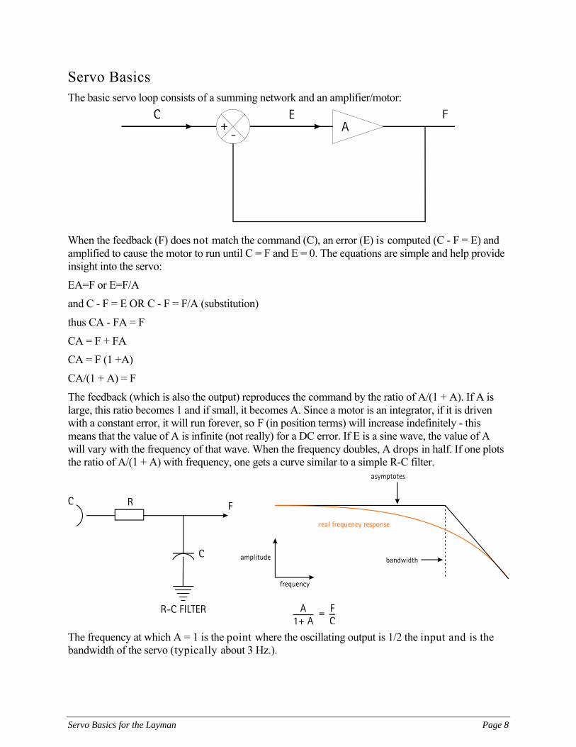
Servo Basics The basic servo loop consists of a summing network and an amplifier/motor:
When the feedback (F) does not match the command (C), an error (E) is computed (C - F = E) and amplified to cause the motor to run until C = F and E = 0. The equations are simple and help provide insight into the servo:
EA=F or E=F/A
and C - F = E OR C - F = F/A (substitution)
thus CA - FA = F
CA = F + FA
CA = F (1 +A)
CA/(1 + A) = F
The feedback (which is also the output) reproduces the command by the ratio of A/(1 + A). If A is large, this ratio becomes 1 and if small, it becomes A. Since a motor is an integrator, if it is driven with a constant error, it will run forever, so F (in position terms) will increase indefinitely - this means that the value of A is infinite (not really) for a DC error. If E is a sine wave, the value of A will vary with the frequency of that wave. When the frequency doubles, A drops in half. If one plots the ratio of A/(1 + A) with frequency, one gets a curve similar to a simple R-C filter.
The frequency at which A = 1 is the point where the oscillating output is 1/2 the input and is the bandwidth of the servo (typically about 3 Hz.).
Servo Basics for the Layman Page 8
The gain of a servo is A and is often expressed in inches per minute per mil (IPM/MIL). This is how fast it will go in IPM with one milliinch (MIL) of error (0.001"). Typically 1 IPM/MIL is common for heavy industrial equipment. At 10 IPM, the error (often called lag) will be 0.01" and at 50 IPM will be 0.05", etc. for a 1 IPM/MIL gain.
Servo Basics for the Layman Page 9
Master/Slave Coordination Writer's note: BULL will be the title of this regular column which will be written in response to readers' questions and concerns regarding motion control and servos. The title was chosen, of course, because it is the first four letters of my last name, not because it is what you can expect to find when you read the column. Nor was it chosen because it describes, in conjunction with a China shop, my style of management; as some might suggest.
In responding to your inquiries, 1 will rely upon my MSEE in Control Theory and Servos and my experience in the numerical control of machines and motion; which includes 17 years in R & D, seven years in sales and marketing management, and four years in general management.
The last article addressed basic questions on Motion Control and resulted in several inquiries about the master/slave form of coordinated motion, which will be discussed below.
Oftentimes, a number of axes need to be operated in synchronism while allowing the entire process to slow down or speed up at the operator's discretion. The most precise way of doing this is to digitally monitor the primary or master axis and to slave all other motions to it. The operator is allowed to change speed or position of the master axis and each slave will maintain its relationship to the master. Historically, if one had several machines in a line whose cycles had to start, move, and stop in precise synchronism, one would mechanically couple the machines through gears and line shafts.
There are several disadvantages to this:
• The machines must be close together.
• The ratio by which the slave follows the master requires physically replacing gears to change.
• Shifting the "phase" between master and slave requires a complicated design.
• Decoupling undesirable mechanical characteristics from one machine to the other is difficult.
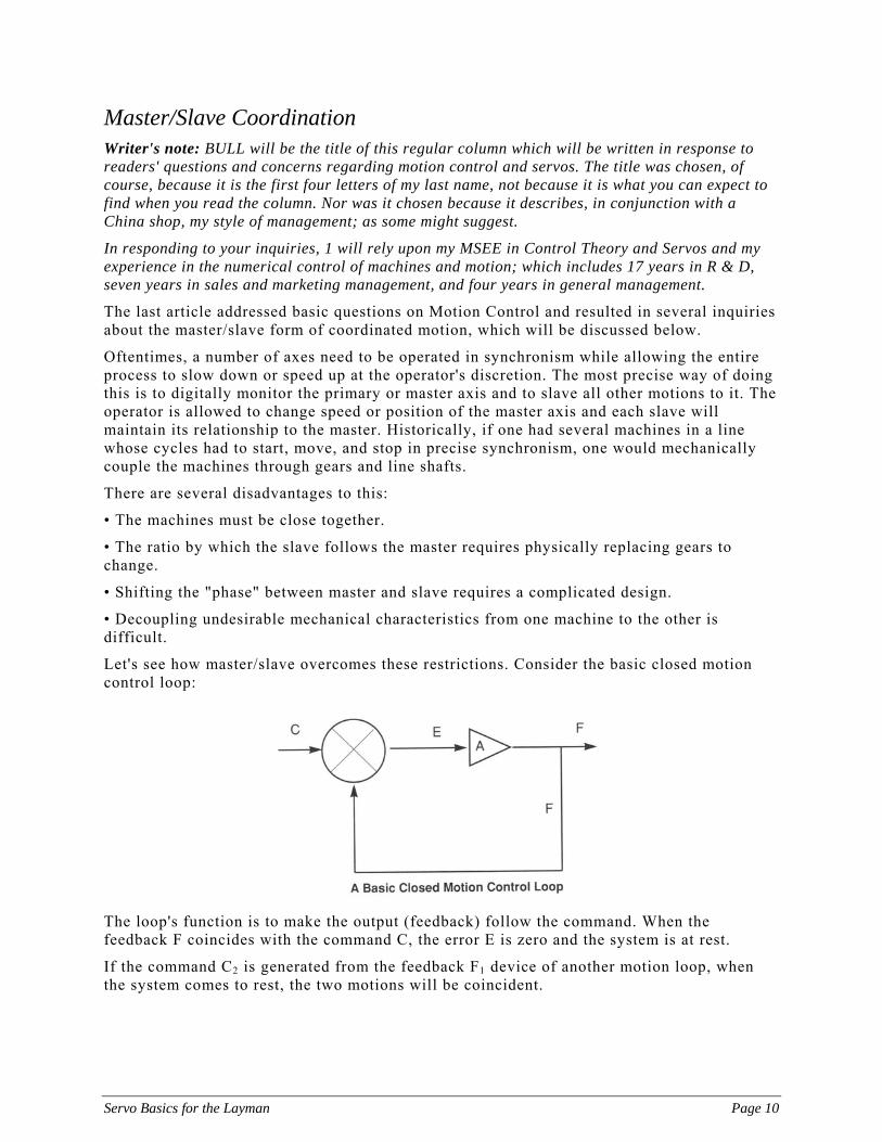
Let's see how master/slave overcomes these restrictions. Consider the basic closed motion control loop:
The loop's function is to make the output (feedback) follow the command. When the feedback F coincides with the command C, the error E is zero and the system is at rest.
If the command C2 is generated from the feedback F1 device of another motion loop, when the system comes to rest, the two motions will be coincident.
Servo Basics for the Layman Page 10
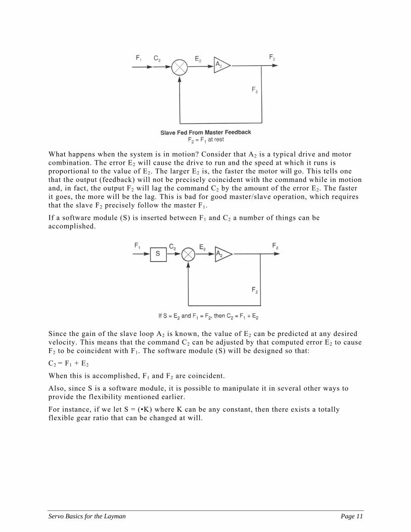
What happens when the system is in motion? Consider that A2 is a typical drive and motor combination. The error E2 will cause the drive to run and the speed at which it runs is proportional to the value of E2. The larger E2 is, the faster the motor will go. This tells one that the output (feedback) will not be precisely coincident with the command while in motion and, in fact, the output F2 will lag the command C2 by the amount of the error E2. The faster it goes, the more will be the lag. This is bad for good master/slave operation, which requires that the slave F2 precisely follow the master F1.
If a software module (S) is inserted between F1 and C2 a number of things can be accomplished.
Since the gain of the slave loop A2 is known, the value of E2 can be predicted at any desired velocity. This means that the command C2 can be adjusted by that computed error E2 to cause F2 to be coincident with F1. The software module (S) will be designed so that:
C2 = F1 + E2
When this is accomplished, F1 and F2 are coincident.
Also, since S is a software module, it is possible to manipulate it in several other ways to provide the flexibility mentioned earlier.
For instance, if we let S = (•K) where K can be any constant, then there exists a totally flexible gear ratio that can be changed at will.
Servo Basics for the Layman Page 11
If, instead of multiplying by a constant, one adds a constant, a phase shift results. The command to the slave can be "shifted" so it lags or leads F, by any desired amount.
It is also possible to filter the input to the second loop:
This can be accomplished with a "digital filter" and allows filtering out any undesirable cyclical variations that may occur in the first motion device (such as vibrations caused by resonances, tools, motors, etc.).
By properly designing the software module (S), one can:
• Provide instant "gear changing."
• Provide flexibility on "gear ratio."
• Shift the position relationship by a constant value.
• Decouple undesirable characteristics.
• Cause several axes to follow the master.
• Allow a complex relationship of the slave to the master over one cycle of the master.
The main purpose of this discussion was to provide an understanding of the master/slave concept and the types of features and solutions that it can provide for you. It will help you to understand your vendor's offerings and to communicate with them.
Your calls and letters are welcome and I will continue to write on those items that you tell me are "hot." And no BULL, either.
Servo Basics for the Layman Page 12
The Bode Diagram Many users of motion control have heard vendors try to explain certain servo features by using Bode diagrams. A basic understanding of them is necessary in dealing with motion. To begin with, the proper pronunciation is "Bo-dee". Just think of Bo Derek (which isn't hard to do). You'll find other similarities between the two (who am I kidding?) like the number 10, as will be seen.
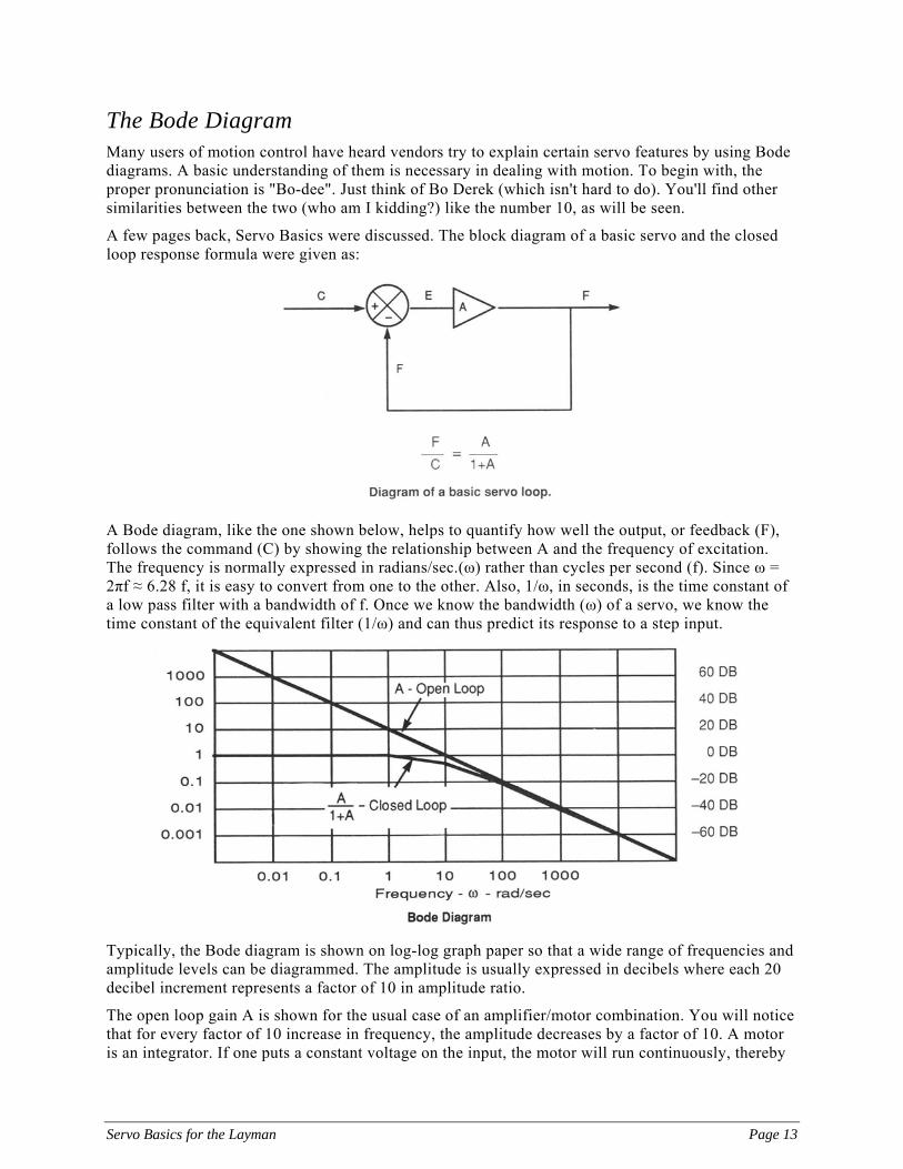
A few pages back, Servo Basics were discussed. The block diagram of a basic servo and the closed loop response formula were given as:
A Bode diagram, like the one shown below, helps to quantify how well the output, or feedback (F), follows the command (C) by showing the relationship between A and the frequency of excitation. The frequency is normally expressed in radians/sec.(ω) rather than cycles per second (f). Since ω = 2πf ≈ 6.28 f, it is easy to convert from one to the other. Also, 1/ω, in seconds, is the time constant of a low pass filter with a bandwidth of f. Once we know the bandwidth (ω) of a servo, we know the time constant of the equivalent filter (1/ω) and can thus predict its response to a step input.
Typically, the Bode diagram is shown on log-log graph paper so that a wide range of frequencies and amplitude levels can be diagrammed. The amplitude is usually expressed in decibels where each 20 decibel increment represents a factor of 10 in amplitude ratio.
The open loop gain A is shown for the usual case of an amplifier/motor combination. You will notice that for every factor of 10 increase in frequency, the amplitude decreases by a factor of 10. A motor is an integrator. If one puts a constant voltage on the input, the motor will run continuously, thereby
Servo Basics for the Layman Page 13
integrating the position to infinity. If one puts a sine wave alternating signal on the motor input, it will cycle back and forth to the same velocity levels, but the position covered during the excursions will vary dramatically with frequency. The higher the frequency, the less time for the excursions to the same velocity levels, and the less distance covered.
Without writing equations, this helps to intuitively explain why A is graphed as shown. One other observation that needs to be made for later use is that the position output lags in phase by 90° from the signal input.
Intuitively, this is obvious when one realizes that the motor will continue in the same positional direction until the input changes polarity to start it on its positional excursion in the other direction. The net effect that needs to be understood is that A is really A∠-90° (it has a gain factor of A and a phase lag of 90°). This Bode plot of A happens to have a gain of 1 (0 DB) at 10 radians/second (≈1.6 cycles/second). The gain adjustment would simply shift the A plot up or down.
The closed loop response [F/C = A/(1+A)] can also be plotted on the Bode diagram. When A is very large, F/C ≈ 1 and when A is very small, F/C ≈ A, which makes it easy to plot F/C except in the vicinity of A = 1. At the A = 1 point, the closed loop gain becomes A∠-90°/(1 + A∠-90°) (Remember that it is 90° phase shifted). In order to add two quantities that are phase shifted by 90°, it is necessary to view them as a right triangle. In this case, with legs of 1 and a magnitude of √2= 1.414
Since 0.707 is -3 DB, the closed loop bandwidth is defined as the point where the magnitude is 3 DB down from where it would be at very low frequencies.
Servo Basics for the Layman Page 14
Making these same calculations for other values of A near the A = 1 point (A = 1/4, 1/2, 2, 4) allows completion of the closed loop frequency response.
The closed loop response is similar to a simple R-C filter with a time constant of 1/ω (0.1 seconds in this case). This allows one to predict the servo's response to a step input in position by referring to texts on simple R-C filters.
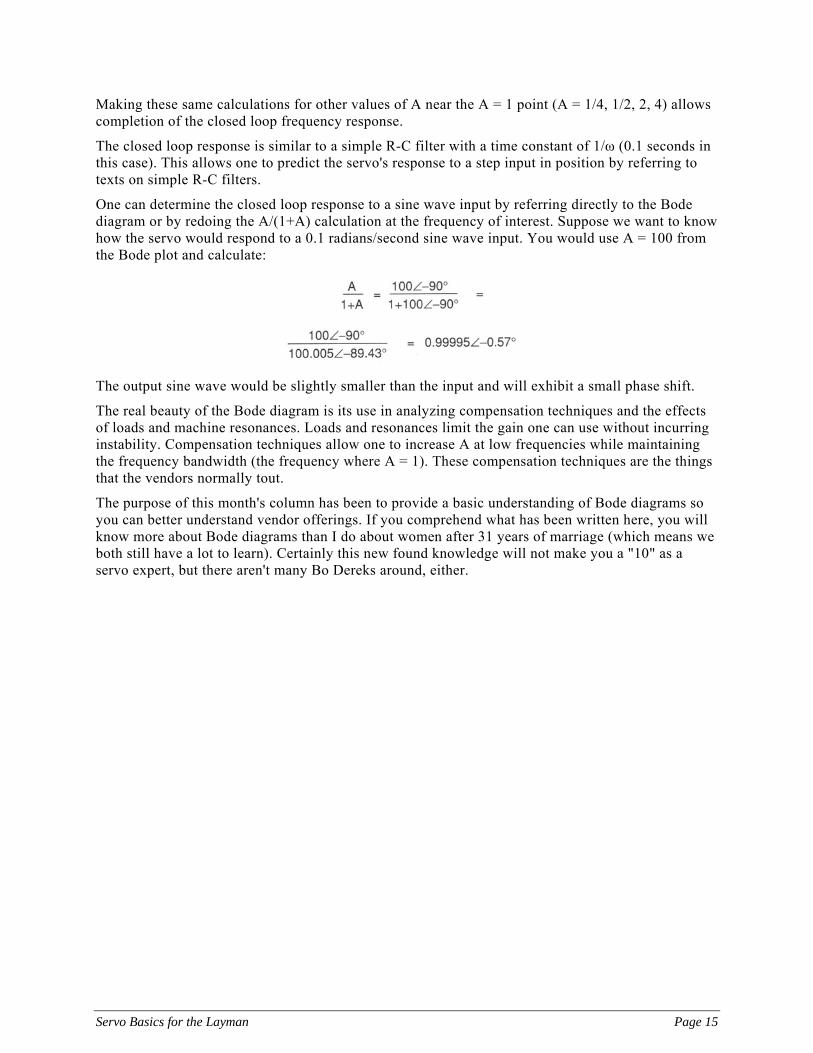
One can determine the closed loop response to a sine wave input by referring directly to the Bode diagram or by redoing the A/(1+A) calculation at the frequency of interest. Suppose we want to know how the servo would respond to a 0.1 radians/second sine wave input. You would use A = 100 from the Bode plot and calculate:
The output sine wave would be slightly smaller than the input and will exhibit a small phase shift.
The real beauty of the Bode diagram is its use in analyzing compensation techniques and the effects of loads and machine resonances. Loads and resonances limit the gain one can use without incurring instability. Compensation techniques allow one to increase A at low frequencies while maintaining the frequency bandwidth (the frequency where A = 1). These compensation techniques are the things that the vendors normally tout.
The purpose of this month's column has been to provide a basic understanding of Bode diagrams so you can better understand vendor offerings. If you comprehend what has been written here, you will know more about Bode diagrams than I do about women after 31 years of marriage (which means we both still have a lot to learn). Certainly this new found knowledge will not make you a "10" as a servo expert, but there aren't many Bo Dereks around, either.
Servo Basics for the Layman Page 15
PID and Servos PID is an acronym that gets used more and more as factory automation requires ever better performance from processes, machines and motion control. There exists a great deal of misunderstanding about it. This article will talk about PID conceptually and practically so that a clearer understanding may prevail.
To begin with, PID means Proportional, Integral and Differential. It probably should have been called IPD rather than PID because the Integral term is most effective at low frequencies, the Proportional term at moderate frequencies, and the Differential term at higher frequencies. These frequencies are relative to the bandwidth of the servo or process.
PID has been much more common in process control where temperatures, pressures, etc. need to be optimally controlled. The primary benefit from the Integral term is the reduction of steady state error while the Differential term helps improve the responsiveness and stability. The theory is valid whether one is controlling temperature, pressure or position. A big difference between a typical process closed loop and a typical position closed loop is the dynamics or frequency response. It is not unusual for a positioning servo to have a bandwidth of 10 Hz or for a process loop to have a bandwidth of 0.1 Hz. Control of temperature, pressure, etc. is usually a "slower" process than positioning with motors.
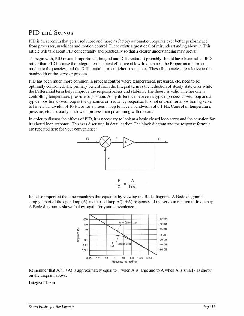
In order to discuss the effects of PID, it is necessary to look at a basic closed loop servo and the equation for its closed loop response. This was discussed in detail earlier. The block diagram and the response formula are repeated here for your convenience:
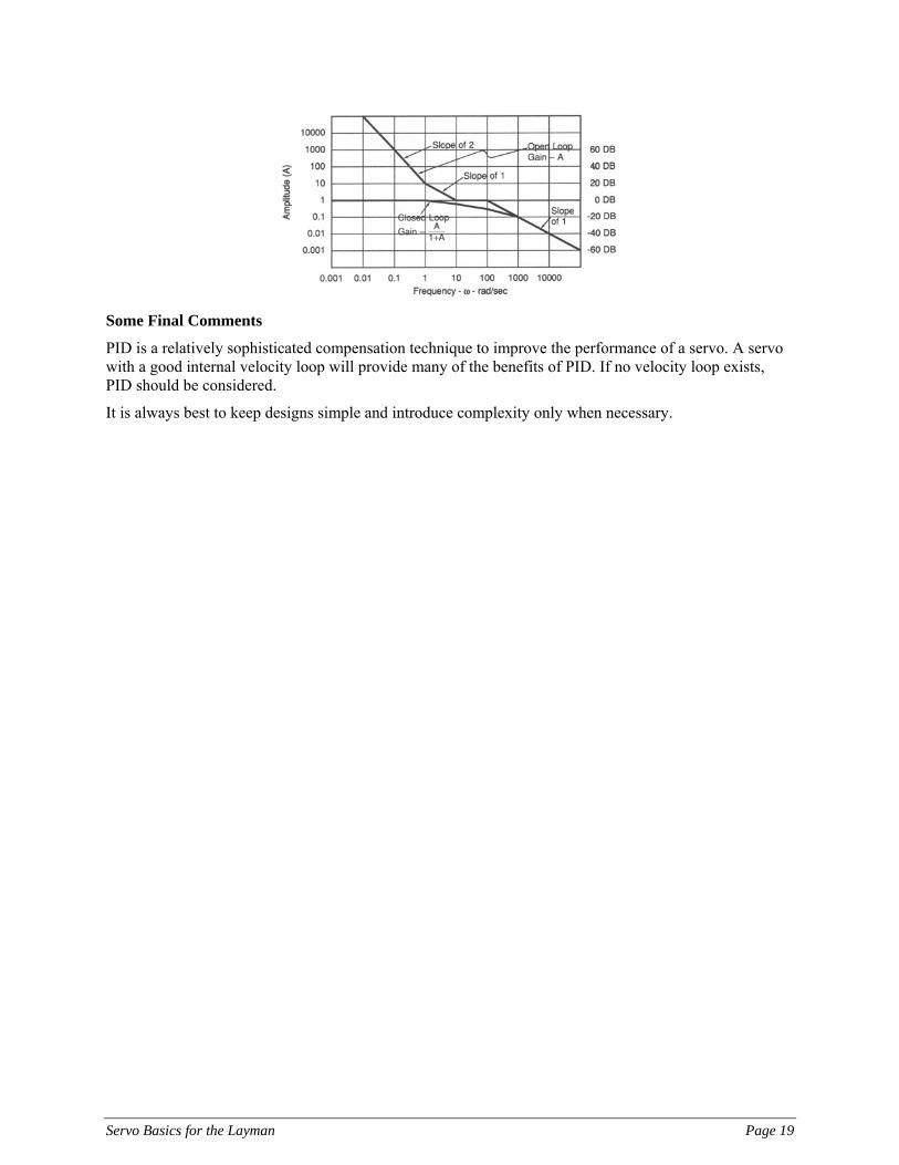
It is also important that one visualizes this equation by viewing the Bode diagram. A Bode diagram is simply a plot of the open loop (A) and closed loop A/(1 +A) responses of the servo in relation to frequency. A Bode diagram is shown below, again for your convenience.
Remember that A/(1 +A) is approximately equal to 1 when A is large and to A when A is small - as shown on the diagram above.
Let's discuss why one might want to introduce an Integral factor into the gain (A) of the control. The Bode diagram shows A approaching infinity as the frequency approaches zero. Theoretically, it does go to infinity at DC because if one put a small error into an open loop drive/motor combination to cause it to move, it would continue to move forever (the position would get larger and larger). This is why a motor is classified as an integrator itself - it integrates the small position error. If one closes the loop, this has the effect of driving the error to zero since any error will eventually cause motion in the proper direction to bring F into coincidence with C. The system will only come to rest when the error is precisely zero! The theory sounds great, but in actual practice the error does not go to zero. In order to cause the motor to move, the error is amplified and generates a torque in the motor. When friction is present, that torque must be large enough to overcome that friction. The motor stops acting as an integrator at the point where the error is just below the point required to induce sufficient torque to break friction. The system will sit there with that error and torque, but will not move.
One can introduce another Integrator (the motor being the first one) at the error point which recognizes and acts upon the least significant increment of the error. As long as an error exists, it will integrate (continually sum) that error (within certain limits) until motion takes place. A second Integrator shows up on a Bode diagram with a plot of gain (A') that has twice the slope previously shown. In the Bode diagram previously shown which has a bandwidth of 10 rad/sec., the double slope would result, for instance, in a gain of 10,000 at 0.1 rad/sec. instead of the 100. This means that the low frequency dynamics are dramatically improved in addition to the error being greatly reduced.
Proportional Term
There is a big problem with A' having two integrators, however. As discussed earlier, an integrator results in its output being 90° phase lagged from its input. By putting two integrators in series, a 180° phase lag results (expressed as A'∠-180°). Under this condition, the closed loop gain becomes:
As A' approaches 1 on the Bode diagram (at 10 rad/sec. in the example), the denominator becomes 1 + 1∠-180° = 1-1 = 0 and F/C becomes infinite! This will result in severe oscillations. In order to maintain a stable system, the denominator must not be allowed to approach 0. When the term "phase margin" is used, it expresses how close the phase shift of A' is to -180° when A' = 1 in magnitude. A commonly accepted design goal is for A' to have -135° of phase shift or less (45° of phase margin). This will result in a 25 percent overshoot of the closed loop system in response to small step inputs in position as shown below.
As the phase margin gets larger, the amount and number of overshoots diminish. As the phase margin gets smaller, the overshoots get larger and will "ring" for longer periods until finally constant "ringing" or sustained oscillation will occur.
In order to remain stable and limit the overshoot response to a step input, the second Integrator must be removed in the vicinity of A' = 1 or in the vicinity of 10 rad/sec. This will allow the phase to approach the -90° associated with the single integration of the motor. Typically, the "break point" at which the Integrator would be removed would be about a factor of 10 from the bandwidth. In the example, the "break point" would be placed at 1 rad/sec. and for frequencies above that value, the compensation for the loop would revert from an Integrator to a Proportional or constant term. If this Proportional term equals 1, then the gain reverts back to A at frequencies above 1 rad/sec. with only the normal single integration caused by the motor.
The methods for making an Integrator and removing it above a specific frequency value are covered in texts on digital filtering or analog filters depending on whether the servo error (E) is digital or analog.
Differential Term
The Integral and Proportional terms have provided a system which is considerably more accurate and responsive at lower frequencies, yet stable based on the phase margin criterion near servo bandwidth frequencies. It may also be desirable to further improve the phase margin so that the bandwidth can be extended or the overshoot of the step response minimized.
This is possible by introducing positive phase to improve the phase margin by means of a Differentiator. Earlier it was mentioned that an Integrator results in the output lagging the input by 90°. Conversely, a Differentiator has an output that leads the input by 90°. An Integrator, with frequency, takes the form of (KI/ω)∠-90° with its gain decreasing with frequency and its output having a 90° phase lag. A Differentiator takes the form KDω∠+90° with its gain increasing with frequency, but its output having a 90° phase lead. By designing the Differentiator so that it is effective for frequencies of 10 rad/sec. and above in the example, the phase lead will benefit the phase margin near the bandwidth frequencies. There is an undesirable effect from this, however. Since the Differentiator causes the gain to increase with frequency, it also increases some of the machine resonances that will often be found in the 100 to 1,000 rad/sec. range. For this reason, the Differentiator is usually "disengaged" back to Proportional at some midpoint between the servo bandwidth and the frequency of the first resonance.
PID
A Bode diagram of the whole PID compensation network would be:
Combining this with the Bode diagram shown earlier for the "naked" loop illustrates that this PID compensation has resulted in a closed loop servo with a wider bandwidth and a greater gain (thus accuracy) within that bandwidth.
Servo Basics for the Layman Page 18
Some Final Comments
PID is a relatively sophisticated compensation technique to improve the performance of a servo. A servo with a good internal velocity loop will provide many of the benefits of PID. If no velocity loop exists, PID should be considered.
It is always best to keep designs simple and introduce complexity only when necessary.
Servo Basics for the Layman Page 19
Servo Types No matter what is dealt with in life, it seems that it must be named and classified - servos are no exception. Servos are classified into three types: type 0, type 1, and type 2. This column will be devoted to discussing these three types plus the advantages and disadvantages of each.
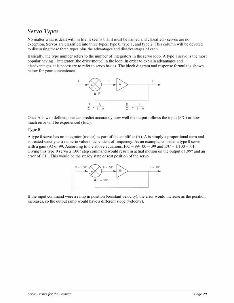
Basically, the type number refers to the number of integrators in the servo loop. A type 1 servo is the most popular having 1 integrator (the drive/motor) in the loop. In order to explain advantages and disadvantages, it is necessary to refer to servo basics. The block diagram and response formula is shown below for your convenience.
Once A is well defined, one can predict accurately how well the output follows the input (F/C) or how much error will be experienced (E/C).
Type 0
A type 0 servo has no integrator (motor) as part of the amplifier (A). A is simply a proportional term and is treated strictly as a numeric value independent of frequency. As an example, consider a type 0 servo with a gain (A) of 99. According to the above equations, F/C = 99/100 = .99 and E/C = 1/100 = .01. Giving this type 0 servo a 1.00" step command would result in actual motion on the output of .99" and an error of .01". This would be the steady state or rest position of the servo.
If the input command were a ramp in position (constant velocity), the error would increase as the position increases, so the output ramp would have a different slope (velocity).
Servo Basics for the Layman Page 20
The conclusion is that a type 0 system does not accurately follow steps in position nor constant velocity commands (position ramps).
Type 1
A type 1 servo has an integrator (motor) as part of the amplifier, so the A term takes the form (KI/ω)∠-90° as discussed in previously. As the frequency (ω) increases, the gain decreases. As the frequency decreases, the gain increases and approaches ∞ when ω approaches 0.
In the steady state condition, the error (E) must approach 0 since the gain (A) approaches ∞. The result of a 1.00" step command would be a final output of 1.00" and an error of 0".
If the input command is a ramp in position (constant velocity), the output will be a ramp in position of precisely the same value (velocity), but lagged in position. This is true because a motor or integrator puts out a position ramp (or velocity) with a constant error (voltage) applied to it. In the steady state (after acceleration is over) the actual position (F) will lag the command (C) by the error (E), but the velocities (ramp slope) of C and F will be identical.
There are two major advantages of a type 1 system over type 0. The steady state error at rest is 0 and it responds precisely in velocity to constant velocity input commands (position ramps).
Type 2
Servo Basics for the Layman Page 21
A type 2 servo has two integrators (usually one motor and one "software" integrator) as part of the amplifier. The A term takes the form (KI/ω2)∠-180°. Since the A term approaches ∞ as ω approaches 0, there will be no error (E) when the system is at rest. In this respect, it is similar to the type 1 servo.
If one considers the condition when a position ramp (constant velocity) is commanded, there are two logical inferences that can be made. The second integrator (the motor) must have a constant input to provide a velocity output. This means that the first integrator needs to supply a constant signal to the second integrator, thus the input to the first integrator must be 0. If the input to the first integrator is 0, then there is no position error in this system in the constant velocity mode. This is exactly the case and explains why so much effort has gone into developing type 2 systems.
In addition to no position error at rest, a type 2 system has the additional feature of no position error with a steady state ramp input in position (after the acceleration is complete.)
Final Comments
It would appear that one should simply use a type 2 servo. Needless to say, it isn't that easy. A type 2 servo is inherently unstable. One must use compensation techniques to make it a type 2 servo which converts to a type 1 near bandwidth frequencies where stability is determined. The earlier discussion on PID described just such a technique to give the low frequency benefits of a type 2 servo, yet achieve stability.
If zero position error is important under steady state positional ramping (constant velocity) conditions, then the PID approximation of a type 2 system is the answer. Don't complicate the design if you don't need it, though.
An example of the need for zero position error would be in master/slave applications where the slave is expected to stay in precise position synchronism with the master even though an operator may choose to change the "speed" of the master.
So much for this class in classifying servos.
Servo Basics for the Layman Page 22
Adjusting PID Gains An earlier discussion explained PID and showed the Bode diagram (open loop gain as a function of frequency) for it. A number of users of PID have indicated that they have difficulty adjusting the gains (KP for the proportional gain, KI for the integral gain, and KD for the differential gain). This reminds me of the golfer on the first tee whose first three swings resulted in nothing but air and whose fourth swing dribbled down the fairway. He turned to his friends and said, "This is a difficult course, isn't it?" It was only difficult because he didn't understand the basics and hadn't practiced them.
This discussion will concentrate on the basics - what happens when you adjust each of the three factors? It will still take some practice to do it well and quickly - and you may never become a 300 yard hitter, but your score will improve dramatically!
Two Bode diagrams from the earlier discussion will be used to help gain a picture of what happens when each of the factors is adjusted. The first Bode plot to be used is of the PID network by itself. Later, a Bode diagram of the total loop gain incorporating the motor (which is also an integrator) will be shown.
The PID network is shown below illustrating the effect of changing only the proportional factor (KP). As can be seen, increasing KP not only increases the mid-frequency range proportional factor, but also lowers the frequency at which the integration factor ceases effectiveness and raises the frequency at which the differential factor begins to kick in. The effect of lowering KP is also illustrated.
Changing the integration factor (KI) has the impact shown below. Not only does it affect the low frequency gain, but it changes the frequency at which the proportional factor (KP) becomes effective. It would be most desirable to raise KI as high as possible, but the higher it gets, the more negative a phase shift is introduced in the proportional range where the servo bandwidth normally ends up. This reduces the phase margin of the servo, causing overshoots and ringing as described in an earlier column.
Increasing the differential gain (KD) lowers the frequency at which it has more impact than the proportional factor (KP). This introduces positive phase shift in the proportional range to help offset the negative phase shift from the integration factor KI, thereby improving the phase margin and reducing the ringing. It has the
Servo Basics for the Layman Page 23
undesirable effect, however, of increasing the high frequency gain, making the servo more noise sensitive and encouraging the undesirable effects of natural resonances.
Now that one can "see" the impact of changing each of the gain factors, it is important to have a procedure to follow when working with them all together.
The Bode diagram that follows, shows the loop gain with the PID plus the integration resulting from the motor. It also shows the effect of increasing each of the three PID gain factors.
The adjustment procedure that seems most logical is first to reduce KI and KD to their minimum values so that KP and thus the servo bandwidth (0 DB crossover frequency) can be set with no influence from the integrator or the differentiator. This KP factor should be set about 30% below the adjustment where instability occurs. Next raise KI until the servo is just below instability, then increase KD to improve the phase margin and system stability. This can be done by repeatedly making about a 30% increase in KD, and then adjusting KI to see if it is still on the edge of instability. When KI no longer appears on the edge of stability, round 1 of the procedure is complete. Now, again increase KI to the point just below instability and again increase KD as before while "testing" KI. This time, when satisfactory operation occurs, the adjustment is complete.
The strategy behind this procedure is first to set the bandwidth for a normal, naked loop without compensation. Once this is done, it is desirable to raise KI as high as possible to approach a type 2 system with two integrators. KI is set as high as is dared and then the positive phase margin from the differential factor is introduced to restore stable operation. This technique is repeated to "tighten up" the proportional gain frequency section. It does not pay to continue to try to optimize since it is too easy to lose the "vision" and balance between KI and KD.
It seems that every time I get my golf game in balance, I start trying new things to make it even better and end up hacking instead of golfing. It usually requires going back to the basics to once again achieve that balance.
Servo Basics for the Layman Page 24
Servo Basics for the Layman Page 25
When you adjust your PID, remember the basics, keep a vision of what is happening, and maintain a balance.
Good luck in adjusting your PID - and your golf game.