Set Theory as a Computational Logic: I. From Foundations to Functions * Lawrence C. Paulson Computer Laboratory University of Cambridge 4 November 1992 Abstract Zermelo-Fraenkel (ZF) set theory is widely regarded as unsuitable for au- tomated reasoning. But a computational logic has been formally derived from the ZF axioms using Isabelle. The library of theorems and derived rules, with Isabelle’s proof tools, support a natural style of proof. The paper describes the derivation of rules for descriptions, relations and functions, and discusses interactive proofs of Cantor’s Theorem, the Composition of Homomorphisms challenge [3], and Ramsey’s Theorem [2]. Copyright c 1992 by Lawrence C. Paulson * Research funded by SERC grant GR/G53279 and by the ESPRIT Basic Research Action 3245 ‘Logical Frameworks’. Isabelle has enjoyed long-standing support from the British SERC, dating from the Alvey Programme (grant GR/E0355.7).
Transcript
Set Theory as a Computational Logic:I. From Foundations to Functions∗
Lawrence C. PaulsonComputer Laboratory
University of Cambridge
4 November 1992
Abstract
Zermelo-Fraenkel (ZF) set theory is widely regarded as unsuitable for au-tomated reasoning. But a computational logic has been formally derived fromthe ZF axioms using Isabelle. The library of theorems and derived rules, withIsabelle’s proof tools, support a natural style of proof. The paper describesthe derivation of rules for descriptions, relations and functions, and discussesinteractive proofs of Cantor’s Theorem, the Composition of Homomorphismschallenge [3], and Ramsey’s Theorem [2].
∗Research funded by SERC grant GR/G53279 and by the ESPRIT Basic Research Action 3245‘Logical Frameworks’. Isabelle has enjoyed long-standing support from the British SERC, datingfrom the Alvey Programme (grant GR/E0355.7).
A great many formalisms have been proposed for reasoning about computer systems:Hoare logics, modal/temporal logics, constructive logics, etc. Some are designed tohandle the needs of a specialized problem domain. Others are designed for ease ofimplementation; consider the highly successful Boyer/Moore logic [4], which consistsof a quantifier-free first-order logic augmented with carefully chosen principles ofrecursion.
Specialized logics often have limited expressive power. Since there is no cleardividing line between computational reasoning and arbitrary mathematics, perhapswe should adopt a fully general mathematical formalism — one that has no difficultywith concepts such as infinite objects, equivalence classes or sets of functions. Ageneral formalism may seem impossible to implement effectively, the more so if itmust compete with other logics in their specialized domains. But M. J. C. Gordon’swork demonstrates that higher-order logic, which is a general formalism, can beapplied successfully to specialized domains such as hardware verification [6, 7].
Axiomatic set theory is older and more general than higher-order logic. Canit be used for verification? Set theory is commonly regarded as unworkable. YetNoel [10], Quaife [18] and Saaltink [20], in their different ways, show that complexset theory proofs are possible. Such work seems to require great care and effort; thenext step is to make the proof process easy.
The drawbacks of set theory are well known. It is extremely low-level, withstrange definitions like 〈a, b〉 ≡ {{a}, {a, b}} and 3 ≡ {0, 1, 2}; and since it has noform of information hiding, it admits strange theorems like {a} ∈ 〈a, b〉 and 2 ∈ 3.But to compensate, set theory has tremendous expressive power. Its basic conceptsare few and are widely understood.
Finally, set theory has no type checking — every object is a set — while higher-order logic has infinitely many types. This is the clearest difference between the twoformalisms. Whether type checking is bad or good is perhaps a matter of taste, justas it is with programming languages.
The paper proceeds as follows. The next two sections introduce Isabelle andaxiomatic set theory. Further sections sketch the Isabelle development of basicconcepts such as relations and functions. Next come interactive proofs of threesmall examples: ordered pairing, Cantor’s Theorem, and the Composition of Homo-morphisms challenge [3]. Ramsey’s Theorem, a more realistic example, permits acomparison between Isabelle and other theorem provers [2]. The remaining sectionsdiscuss related work and draw conclusions.
2 Isabelle
The formalization and proofs discussed below have been done with the help of Isa-belle, an interactive theorem prover [14]. Isabelle is generic: it supports a rangeof formalisms, including modal, first-order, higher-order, and intuitionistic logics.Isabelle’s generic capabilities are vital for using set theory, whose axioms are far too
2 ISABELLE 2
low-level for most proofs. Isabelle’s version of set theory includes derived theories ofrelations, functions and type constructions, which can be regarded as logics in theirown right. These theories exploit Isabelle’s treatment of syntax, variable-bindingoperators, and derived rules.
Isabelle works directly with schematic inference rules of the form
[[φ1; . . . ;φn]] =⇒ φ.
Rules are combined by a generalization of Horn clause resolution. Theorems areproved not by refutation, but in the affirmative. Joining rules by resolution con-structs a proof tree, whose root is the conclusion.
Such rules are theorems of Isabelle’s meta-logic, which is a fragment of higher-order logic. The symbol =⇒ is meta-implication; the notation [[φ1; . . . ;φn]] =⇒ φabbreviates
φ1 =⇒ (· · · =⇒ (φn =⇒ φ) · · ·).The symbol
∧is another meta-connective, a universal quantifier, for expressing
generality in rules. The symbol ≡, which is meta-equality, expresses definitions.Elsewhere [12] I discuss how to formalize object-logics in the meta-logic, and howto prove that the formalization is correct.
Expressions in the meta-logic are typed λ-terms, and λ-abstraction handles anobject-logic’s quantifiers and other variable-binding operators. The presence of λ-terms means that Isabelle cannot use ordinary unification. Higher-order unifica-tion is undecidable in the general case but works well in practice — particularly forenforcing quantifier rule provisos of the form ‘x not free in . . . ’ [12].
For backward proof, a rule of the form [[φ1; . . . ;φn]] =⇒ φ can represent a proofstate; the ultimate goal is φ and the subgoals still unsolved are φ1, . . . , φn. Aninitial proof state has the form φ =⇒ φ, with one subgoal, and a final proof statehas the form φ, with no subgoals. The final proof state is itself the desired theorem.
Tactics are functions that transform proof states. A backward proof proceedsby applying tactics in succession to the initial state, reaching a final state. Thetactic resolve_tac performs Isabelle’s form of Horn clause resolution; it attemptsto unify the conclusion of some inference rule with a subgoal, replacing it by therule’s instantiated premises. This is proof checking.
Isabelle also supports automated reasoning. Each tactic maps a proof state to alazy list of possible next states. Backtracking is therefore possible and tactics canimplement search strategies such as depth-first, best-first and iterative deepening.Tacticals are operators for combining tactics. They typically express control struc-tures, ranging from basic sequencing to search strategies. Isabelle provides severalpowerful, generic tools:
• The classical reasoner applies naive heuristics to prove theorems in thestyle of the sequent calculus. Despite its naiveity, it can prove many nontrivialtheorems, including nearly all of Pelletier’s graded problems short of Schubert’sSteamroller [17]. As an interactive tool it is valuable. It is not restricted tofirst-order logic, but exploits any natural deduction rules. It can prove severalkey lemmas for Ramsey’s Theorem [2].
3 SET THEORY 3
• The simplifier applies rewrite rules to a goal, then attempts to prove therewritten goal using a user-supplied tactic. A conditional rewrite rule is ap-plied only if recursive simplification proves the instantiated condition. Con-textual information is also used, rewriting x = t → ψ(x) to x = t → ψ(t).Rewriting works not just for equality, but for any reflexive/transitive rela-tion enjoying congruence laws. Used with the classical reasoner, it can proveBoyer et al.’s challenge problem, that the composition of homomorphisms is ahomomorphism [3].
Isabelle does not find proofs automatically. Proofs require a skilled user, who mustdecide which lemmas to prove and which tools to apply. Each tool must be givena set of appropriate lemmas. For instance, the proof about composition of homo-morphisms requires lemmas about the composition of functions. Sometimes no toolis appropriate and we must use proof checking; even these proofs can be concise ifthey exploit derived rules and tacticals.
3 Set theory
Axiomatic set theory was developed in response to paradoxes such as Russell’s. Setscould not be arbitrary collections of the form {x . φ(x)}, pulled out of a hat. Theyhad to be constructed, starting from a few given sets. Operations for constructingnew sets included union, powerset and replacement.
Replacement is the most powerful set constructor. If A is a set, and the binarypredicate φ(x, y) is single-valued for all x in A, then replacement yields the imageof A under the predicate φ. Formally, if
∀x∈A . ∀y z . φ(x, y) ∧ φ(x, z)→ y = z
then there exists a set R(A, φ) such that
b ∈ R(A, φ)↔ (∃x∈A . φ(x, b)).
Replacement entails the principle of Separation. Let A be a set and ψ(x) a unarypredicate. Separation yields a set, written {x ∈ A . ψ(x)}, consisting of thoseelements of A that satisfy ψ:
a ∈ {x ∈ A . ψ(x)} ↔ a ∈ A ∧ ψ(a)
A class is an arbitrary collection of sets. Elements of the class {x . ψ(x)} are notrestricted to elements of some other set. Every set B is a class, namely {x . x ∈ B}.Many classes are too big to be sets, such as the universal class, V ≡ {x . x = x}.If V were a set then we could obtain Russell’s Paradox via Separation: define theset R ≡ {x ∈ V . x 6∈ x}, then R ∈ R ↔ R 6∈ R. We could define R as a class,namely R ≡ {x . x 6∈ x}, but this yields no paradox because a proper class cannotbe a member of another class: R ∈ R is false.
3 SET THEORY 4
3.1 Which axiom system?
The two main axiom systems for set theory, Zermelo-Fraenkel (ZF) and vonNeumann-Bernays-Godel (NBG), differ in their treatment of classes. In ZF, vari-ables range over sets; classes do not exist at all, but we may regard unary predicatesas classes if we like. In NBG, variables range over classes, and A ∈ V expresses thatthe class A is actually a set. The two axiom systems are similar in strength. Mostset theorists prefer ZF because they are interested in sets, not classes. Moreover,NBG is tiresome to use — it frequently requires showing that certain classes aresets. Even a ∈ {a} holds only if a ∈ V ; see Lemma 9 of Boyer et al. [3].
ZF has one serious drawback: Replacement is expressed by an axiom scheme,parametrized by the predicate φ. A textbook application of the Compactness Theo-rem demonstrates that ZF can have no finite axiom system in first-order logic. Thus,it is unsuitable for first-order resolution theorem provers. Boyer et al. [3] advocateNBG because it is finite. Quaife [18] has simplified their clauses for NBG and provedseveral hundred results, using the resolution prover Otter.
Isabelle can express axiom schemes, since its meta-logic is higher-order. In theaxiom of Replacement, the binary predicate φ is a variable of type [i, i]⇒ o, whichis the type of functions that map two individuals to a truth value. Separation canbe derived in its schematic form, where the unary predicate ψ is a variable of typei⇒ o.
Schemes can nonetheless cause problems with search. The goal
t ∈ ?A,
could be refined, instantiating the unknown ?A (a ‘logical variable’), to the subgoal
t ∈ {x ∈ ?B . ?ψ(x)}.This can be refined, by the principle of Separation, to the two subgoals
t ∈ ?B and ?ψ(t).
The subgoal t ∈ ?B can be refined exactly like t ∈ ?A, making the search loop; thesubgoal ?ψ(t) is totally unconstrained, since it consists of a formula unknown. Hadwe proved t ∈ ?A by instantiating ?A to {t}, we might have invalidated other goalsinvolving ?A. Such a situation arises in the proof of Cantor’s Theorem (see §5.2).Automatic tools seldom cope; the user can help by explicitly instantiating unknownssuch as ?A.
3.2 The Zermelo-Fraenkel axioms in Isabelle
The ZF axioms from Suppes [22, page 238] are expressed using Isabelle’s formulationof classical first-order logic. For clarity, the exposition uses standard mathematicalnotation rather than Isabelle’s ASCII substitutes [16]. We begin by defining thebounded quantifiers:
∀x∈A . P (x) ≡ ∀x . x ∈ A→ P (x)
∃x∈A . P (x) ≡ ∃x . x ∈ A ∧ P (x)
3 SET THEORY 5
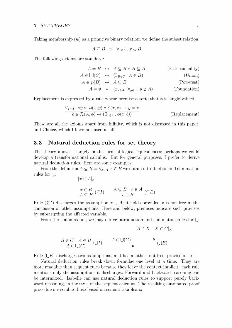
Taking membership (∈) as a primitive binary relation, we define the subset relation:
A ⊆ B ≡ ∀x∈A . x ∈ B
The following axioms are standard:
A = B ↔ A ⊆ B ∧B ⊆ A (Extensionality)
A ∈⋃
(C) ↔ (∃B∈C . A ∈ B) (Union)
A ∈ ℘(B) ↔ A ⊆ B (Powerset)
A = ∅ ∨ (∃x∈A . ∀y∈x . y 6∈ A) (Foundation)
Replacement is expressed by a rule whose premise asserts that φ is single-valued:
∀x∈A . ∀y z . φ(x, y) ∧ φ(x, z)→ y = z
b ∈ R(A, φ)↔ (∃x∈A . φ(x, b)) (Replacement)
These are all the axioms apart from Infinity, which is not discussed in this paper,and Choice, which I have not used at all.
3.3 Natural deduction rules for set theory
The theory above is largely in the form of logical equivalences; perhaps we coulddevelop a transformational calculus. But for general purposes, I prefer to derivenatural deduction rules. Here are some examples.
From the definition A ⊆ B ≡ ∀x∈A.x ∈ B we obtain introduction and eliminationrules for ⊆:
[x ∈ A]x....x ∈ BA ⊆ B
(⊆I)A ⊆ B c ∈ A
c ∈ B (⊆E)
Rule (⊆I) discharges the assumption x ∈ A; it holds provided x is not free in theconclusion or other assumptions. Here and below, premises indicate such provisosby subscripting the affected variable.
From the Union axiom, we may derive introduction and elimination rules for⋃
:
B ∈ C A ∈ BA ∈ ⋃(C)
(⋃I)
A ∈ ⋃(C)
[A ∈ X X ∈ C]X....θ
θ(⋃E)
Rule (⋃E) discharges two assumptions, and has another ‘not free’ proviso on X.
Natural deduction rules break down formulae one level at a time. They aremore readable than sequent rules because they leave the context implicit: each rulementions only the assumptions it discharges. Forward and backward reasoning canbe intermixed. Isabelle can use natural deduction rules to support purely back-ward reasoning, in the style of the sequent calculus. The resulting automated proofprocedures resemble those based on semantic tableaux.
3 SET THEORY 6
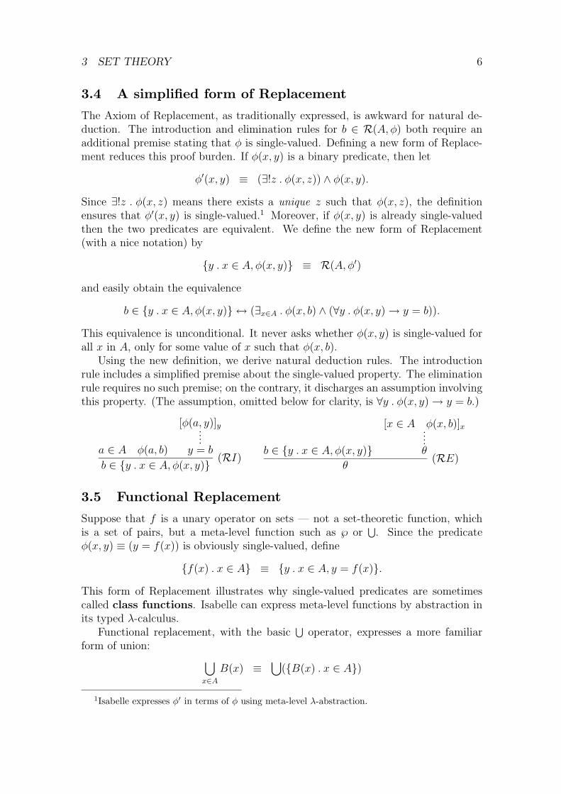
3.4 A simplified form of Replacement
The Axiom of Replacement, as traditionally expressed, is awkward for natural de-duction. The introduction and elimination rules for b ∈ R(A, φ) both require anadditional premise stating that φ is single-valued. Defining a new form of Replace-ment reduces this proof burden. If φ(x, y) is a binary predicate, then let
φ′(x, y) ≡ (∃!z . φ(x, z)) ∧ φ(x, y).
Since ∃!z . φ(x, z) means there exists a unique z such that φ(x, z), the definitionensures that φ′(x, y) is single-valued.1 Moreover, if φ(x, y) is already single-valuedthen the two predicates are equivalent. We define the new form of Replacement(with a nice notation) by
{y . x ∈ A, φ(x, y)} ≡ R(A, φ′)
and easily obtain the equivalence
b ∈ {y . x ∈ A, φ(x, y)} ↔ (∃x∈A . φ(x, b) ∧ (∀y . φ(x, y)→ y = b)).
This equivalence is unconditional. It never asks whether φ(x, y) is single-valued forall x in A, only for some value of x such that φ(x, b).
Using the new definition, we derive natural deduction rules. The introductionrule includes a simplified premise about the single-valued property. The eliminationrule requires no such premise; on the contrary, it discharges an assumption involvingthis property. (The assumption, omitted below for clarity, is ∀y . φ(x, y)→ y = b.)
a ∈ A φ(a, b)
[φ(a, y)]y....y = b
b ∈ {y . x ∈ A, φ(x, y)} (RI)b ∈ {y . x ∈ A, φ(x, y)}
[x ∈ A φ(x, b)]x....θ
θ(RE)
3.5 Functional Replacement
Suppose that f is a unary operator on sets — not a set-theoretic function, whichis a set of pairs, but a meta-level function such as ℘ or
⋃. Since the predicate
φ(x, y) ≡ (y = f(x)) is obviously single-valued, define
{f(x) . x ∈ A} ≡ {y . x ∈ A, y = f(x)}.
This form of Replacement illustrates why single-valued predicates are sometimescalled class functions. Isabelle can express meta-level functions by abstraction inits typed λ-calculus.
Functional replacement, with the basic⋃
operator, expresses a more familiarform of union: ⋃
x∈AB(x) ≡
⋃({B(x) . x ∈ A})
1Isabelle expresses φ′ in terms of φ using meta-level λ-abstraction.
4 DERIVING A THEORY OF FUNCTIONS 7
The corresponding natural deduction rules are
a ∈ A b ∈ B(a)
b ∈ (⋃x∈A .B(x))
(⋃RI)
b ∈ (⋃x∈A .B(x))
[x ∈ A b ∈ B(x)]x....θ
θ(⋃RE)
3.6 Separation
Given a set A and a unary predicate ψ, Separation yields a set consisting of thoseelements of A that satisfy ψ. Separation is easily defined in terms of Replacement:
{x ∈ A . ψ(x)} ≡ {y . x ∈ A, x = y ∧ ψ(x)}
The natural deduction rules have simple derivations:
a ∈ A ψ(a)
a ∈ {x ∈ A . ψ(x)}a ∈ {x ∈ A . ψ(x)}
a ∈ Aa ∈ {x ∈ A . ψ(x)}
ψ(a)
Using Separation, we can define general intersection:⋂(C) ≡ {x ∈
⋃(C) . ∀Y ∈C . x ∈ Y }
The empty intersection,⋂
(∅), causes difficulties. It would like to contain everything,but there is no universal set;
⋂(∅) should be undefined. But Isabelle’s set theory does
not formalize the notion of definedness; all terms are defined. Because⋃
(∅) = ∅, weobtain the perverse (but harmless) result
⋂(∅) = ∅.
4 Deriving a theory of functions
The next developments are tightly linked. We define unordered pairs, then binaryunions and intersections, and obtain finite sets of arbitrary size. Then we can definedescriptions and ordered pairs. Finally, we can define Cartesian products, binaryrelations and functions. The resulting theory includes a sort of λ-calculus with Πand Σ types. All the proofs have been done in Isabelle.
4.1 Finite sets and the boolean operators
Unordered pairing is frequently taken as primitive, but it can be defined in terms ofReplacement [22, page 237]. Observe that ℘(℘(∅)) contains two distinct elements, ∅and ℘(∅).
Upair(a, b) ≡ {y . x ∈ ℘(℘(∅)), (x = ∅ ∧ y = a) ∨ (x = ℘(∅) ∧ y = b)}
Tedious but elementary reasoning yields the key property:
c ∈ Upair(a, b)↔ (c = a ∨ c = b).
4 DERIVING A THEORY OF FUNCTIONS 8
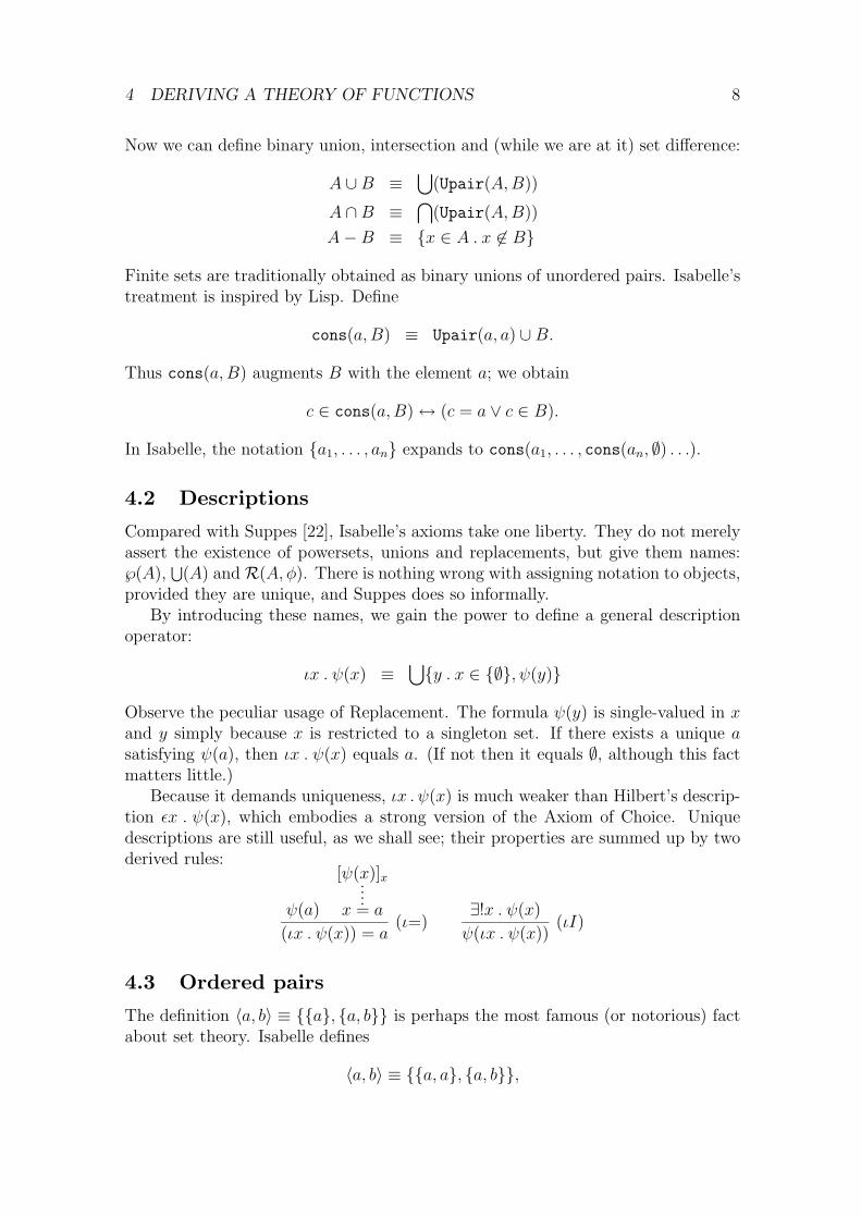
Now we can define binary union, intersection and (while we are at it) set difference:
A ∪B ≡⋃
(Upair(A,B))
A ∩B ≡⋂
(Upair(A,B))
A−B ≡ {x ∈ A . x 6∈ B}
Finite sets are traditionally obtained as binary unions of unordered pairs. Isabelle’streatment is inspired by Lisp. Define
cons(a,B) ≡ Upair(a, a) ∪B.
Thus cons(a,B) augments B with the element a; we obtain
c ∈ cons(a,B)↔ (c = a ∨ c ∈ B).
In Isabelle, the notation {a1, . . . , an} expands to cons(a1, . . . , cons(an, ∅) . . .).
4.2 Descriptions
Compared with Suppes [22], Isabelle’s axioms take one liberty. They do not merelyassert the existence of powersets, unions and replacements, but give them names:℘(A),
⋃(A) andR(A, φ). There is nothing wrong with assigning notation to objects,
provided they are unique, and Suppes does so informally.By introducing these names, we gain the power to define a general description
operator:
ιx . ψ(x) ≡⋃{y . x ∈ {∅}, ψ(y)}
Observe the peculiar usage of Replacement. The formula ψ(y) is single-valued in xand y simply because x is restricted to a singleton set. If there exists a unique asatisfying ψ(a), then ιx . ψ(x) equals a. (If not then it equals ∅, although this factmatters little.)
Because it demands uniqueness, ιx . ψ(x) is much weaker than Hilbert’s descrip-tion εx . ψ(x), which embodies a strong version of the Axiom of Choice. Uniquedescriptions are still useful, as we shall see; their properties are summed up by twoderived rules:
ψ(a)
[ψ(x)]x....x = a
(ιx . ψ(x)) = a(ι=)
∃!x . ψ(x)
ψ(ιx . ψ(x))(ιI)
4.3 Ordered pairs
The definition 〈a, b〉 ≡ {{a}, {a, b}} is perhaps the most famous (or notorious) factabout set theory. Isabelle defines
〈a, b〉 ≡ {{a, a}, {a, b}},
4 DERIVING A THEORY OF FUNCTIONS 9
which is equivalent but consists entirely of doubletons. This simplifies the proof —which we shall examine later — of the key property
〈a, b〉 = 〈c, d〉 ↔ a = c ∧ b = d.
The next step is to define the projections, fst and snd. Descriptions are extremelyuseful here. We could put
fst(p) ≡ ιx . ∃y . p = 〈x, y〉snd(p) ≡ ιy . ∃x . p = 〈x, y〉
To show fst(〈a, b〉) = a by the rule (ι=), we must exhibit a unique x such that∃y . p = 〈x, y〉 holds. Clearly x = a (with y = b) by uniqueness of pairing. Thetreatment of snd is similar. Descriptions are suitable for defining many other kindsof destructors, such as case analysis operators for disjoint unions, natural numbersand lists. Isabelle’s classical reasoner can prove the resulting equations.
Isabelle’s ZF actually defines fst and snd indirectly. Following Martin-Lof’s Constructive Type Theory [11], it defines the variable-binding projectionsplit(p, f), and proves the equation
split(〈a, b〉, f) = f(a, b).
Frequently split is more convenient than the usual projections, which we can defineconcisely:2
fst(p) ≡ split(p, x y . x)
snd(p) ≡ split(p, x y . y)
Like other destructors, split is defined using a description:
split(p, f) ≡ ιz . ∃x y . p = 〈x, y〉 ∧ z = f(x, y).
4.4 Cartesian products
The set A × B consists of all pairs 〈a, b〉 such that a ∈ A and b ∈ B. Manyauthors [8, 22] define the Cartesian product in a cumbersome manner. If a ∈ A andb ∈ B then {{a}, {a, b}} ∈ ℘(℘(A ∪B)), so they define A×B using Separation:
A×B ≡ {z ∈ ℘(℘(A ∪B)) . ∃x∈A . ∃y∈B . z = 〈x, y〉}
There is a historical and pedagogical case for this definition, which postpones theintroduction of Replacement. But Replacement is built into our notation, so wemight as well take advantage of it:
A×B ≡⋃x∈A
⋃y∈B{〈x, y〉}
2Here x y . x and x y . y stand for meta-level λ-abstractions, which would appear as %x y.x and%x y.y in an Isabelle source file.
4 DERIVING A THEORY OF FUNCTIONS 10
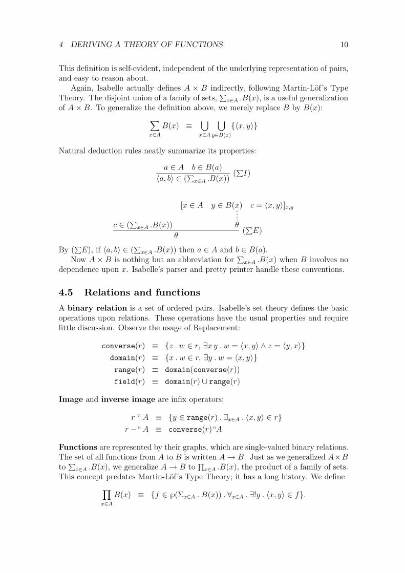
This definition is self-evident, independent of the underlying representation of pairs,and easy to reason about.
Again, Isabelle actually defines A × B indirectly, following Martin-Lof’s TypeTheory. The disjoint union of a family of sets,
∑x∈A .B(x), is a useful generalization
of A×B. To generalize the definition above, we merely replace B by B(x):∑x∈A
B(x) ≡⋃x∈A
⋃y∈B(x)
{〈x, y〉}
Natural deduction rules neatly summarize its properties:
a ∈ A b ∈ B(a)
〈a, b〉 ∈ (∑x∈A .B(x))
(∑I)
c ∈ (∑x∈A .B(x))
[x ∈ A y ∈ B(x) c = 〈x, y〉]x,y....θ
θ(∑E)
By (∑E), if 〈a, b〉 ∈ (
∑x∈A .B(x)) then a ∈ A and b ∈ B(a).
Now A × B is nothing but an abbreviation for∑x∈A .B(x) when B involves no
dependence upon x. Isabelle’s parser and pretty printer handle these conventions.
4.5 Relations and functions
A binary relation is a set of ordered pairs. Isabelle’s set theory defines the basicoperations upon relations. These operations have the usual properties and requirelittle discussion. Observe the usage of Replacement:
converse(r) ≡ {z . w ∈ r, ∃x y . w = 〈x, y〉 ∧ z = 〈y, x〉}domain(r) ≡ {x . w ∈ r, ∃y . w = 〈x, y〉}range(r) ≡ domain(converse(r))
field(r) ≡ domain(r) ∪ range(r)
Image and inverse image are infix operators:
r “ A ≡ {y ∈ range(r) . ∃x∈A . 〈x, y〉 ∈ r}r −“ A ≡ converse(r)“A
Functions are represented by their graphs, which are single-valued binary relations.The set of all functions from A to B is written A→ B. Just as we generalized A×Bto∑x∈A .B(x), we generalize A→ B to
∏x∈A .B(x), the product of a family of sets.
This concept predates Martin-Lof’s Type Theory; it has a long history. We define∏x∈A
Here A → B abbreviates∏x∈A .B(x) when B involves no dependence upon x. In
particular, we have
(f ∈ A→ B)↔ f ⊆ A×B ∧ (∀x∈A . ∃!y . 〈x, y〉 ∈ f).
We further define application and λ-abstraction. An explicit application operatoris necessary; f ‘a operates on the sets f and a. Observe how easily a descriptionexpresses the application operator:
f ‘a ≡ ιy . 〈a, y〉 ∈ fλx∈A . b(x) ≡ {〈x, b(x)〉 . x ∈ A}
Regarding functions as binary relations is tiresome. Only with difficulty can wederive high-level rules for functions, in the style of the λ-calculus.
[x ∈ A]x....b(x) ∈ B(x)
(λx∈A . b(x)) ∈ (∏x∈A .B(x))
(λΠI)f ∈ (
∏x∈A .B(x)) a ∈ Af ‘a ∈ B(a)
(λΠE)
a ∈ A(λx∈A . b(x))‘a = b(a)
(β)f ∈ (
∏x∈A .B(x))
(λx∈A . f ‘x) = f(η)
Injections, surjections and bijections are subsets of the total function space A→ B.Isabelle’s set theory also defines composition of relations (including functions):
inj(A,B) ≡ {f ∈ A→ B . ∀w∈A . ∀x∈A . f ‘w = f ‘x→ w = x}surj(A,B) ≡ {f ∈ A→ B . ∀y∈B . ∃x∈A . f ‘x = y}bij(A,B) ≡ inj(A,B) ∩ surj(A,B)
r ◦ s ≡ {w ∈ domain(s)× range(r) . ∃x y z .w = 〈x, z〉 ∧ 〈x, y〉 ∈ s ∧ 〈y, z〉 ∈ r}
The numerous derived rules include
f ∈ bij(A,B)
converse(f) ∈ bij(B,A)
f ∈ inj(A,B) a ∈ Aconverse(f)‘(f ‘a) = a
s ⊆ A×B r ⊆ B × C(r ◦ s) ⊆ A× C
g ∈ A→ B f ∈ B → C
(f ◦ g) ∈ A→ C
(r ◦ s) ◦ t = r ◦ (s ◦ t)Thus, relations and functions are closed under composition. A similar property isproved for injections, surjections and bijections.
5 EXAMPLES OF SET-THEORETIC REASONING 12
5 Examples of set-theoretic reasoning
To give some idea of the level of reasoning possible in Isabelle, we shall examinethree simple examples: ordered pairing, Cantor’s Theorem, and the Compositionof Homomorphisms challenge [3]. The sessions given below are based on polishedproofs from Isabelle’s set theory. I have simplified the commands to make the proofsslightly longer and easier to follow.
This section, which is intended for casual reading, describes the effect of eachcommand in general terms. For details of the many Isabelle primitives that appear,please consult the documentation [15].
5.1 Injectivity of ordered pairing
Proving that 〈a, b〉 ≡ {{a, a}, {a, b}} is a valid definition of ordered pairing is tire-some — see Halmos [8, page 23], for example. Here is a short machine proof usingIsabelle’s tools. We do not see all the details of a full proof (that happens internally)but we do see the key lemma. We now state this lemma, which concerns doubletons,to Isabelle:
1. {a,b} = {c,d} <-> a = c & b = d | a = d & b = c
This is the initial state of a backward proof. It has one subgoal, which is the sameas the main or ultimate goal. Our first inference will apply the derived rule
P ↔ Q Q↔ RP ↔ R
to let us replace {a, b} = {c, d} by any equivalent formula:
by (resolve_tac [iff_trans] 1);Level 1
{a,b} = {c,d} <-> a = c & b = d | a = d & b = c
1. {a,b} = {c,d} <-> ?Q
2. ?Q <-> a = c & b = d | a = d & b = c
The one subgoal has become two, and the unknown intermediate formula appearsas ?Q. The first occurrence of = in the main goal is one of the rare cases whenthe Axiom of Extensionality is directly useful. We replace {a, b} = {c, d} by theinclusions {a, b} ⊆ {c, d} and {c, d} ⊆ {a, b}, updating ?Q.
by (resolve_tac [extension] 1);Level 2
{a,b} = {c,d} <-> a = c & b = d | a = d & b = c
1. {a,b} <= {c,d} & {c,d} <= {a,b} <-> a = c & b = d | a = d & b = c
5 EXAMPLES OF SET-THEORETIC REASONING 13
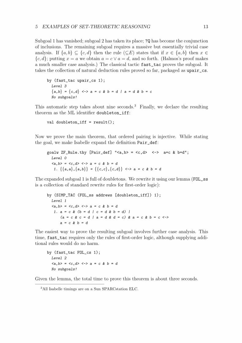
Subgoal 1 has vanished; subgoal 2 has taken its place; ?Q has become the conjunctionof inclusions. The remaining subgoal requires a massive but essentially trivial caseanalysis. If {a, b} ⊆ {c, d} then the rule (⊆E) states that if x ∈ {a, b} then x ∈{c, d}; putting x = a we obtain a = c ∨ a = d, and so forth. (Halmos’s proof makesa much smaller case analysis.) The classical tactic fast_tac proves the subgoal. Ittakes the collection of natural deduction rules proved so far, packaged as upair_cs.
by (fast_tac upair_cs 1);Level 3
{a,b} = {c,d} <-> a = c & b = d | a = d & b = c
No subgoals!
This automatic step takes about nine seconds.3 Finally, we declare the resultingtheorem as the ML identifier doubleton_iff:
val doubleton_iff = result();
Now we prove the main theorem, that ordered pairing is injective. While statingthe goal, we make Isabelle expand the definition Pair_def:
1. {{a,a},{a,b}} = {{c,c},{c,d}} <-> a = c & b = d
The expanded subgoal 1 is full of doubletons. We rewrite it using our lemma (FOL_ssis a collection of standard rewrite rules for first-order logic):
by (SIMP_TAC (FOL_ss addrews [doubleton_iff]) 1);Level 1
<a,b> = <c,d> <-> a = c & b = d
1. a = c & (b = d | c = d & b = d) |
(a = c & c = d | a = d & d = c) & a = c & b = c <->
a = c & b = d
The easiest way to prove the resulting subgoal involves further case analysis. Thistime, fast_tac requires only the rules of first-order logic, although supplying addi-tional rules would do no harm.
by (fast_tac FOL_cs 1);Level 2
<a,b> = <c,d> <-> a = c & b = d
No subgoals!
Given the lemma, the total time to prove this theorem is about three seconds.
3All Isabelle timings are on a Sun SPARCstation ELC.
5 EXAMPLES OF SET-THEORETIC REASONING 14
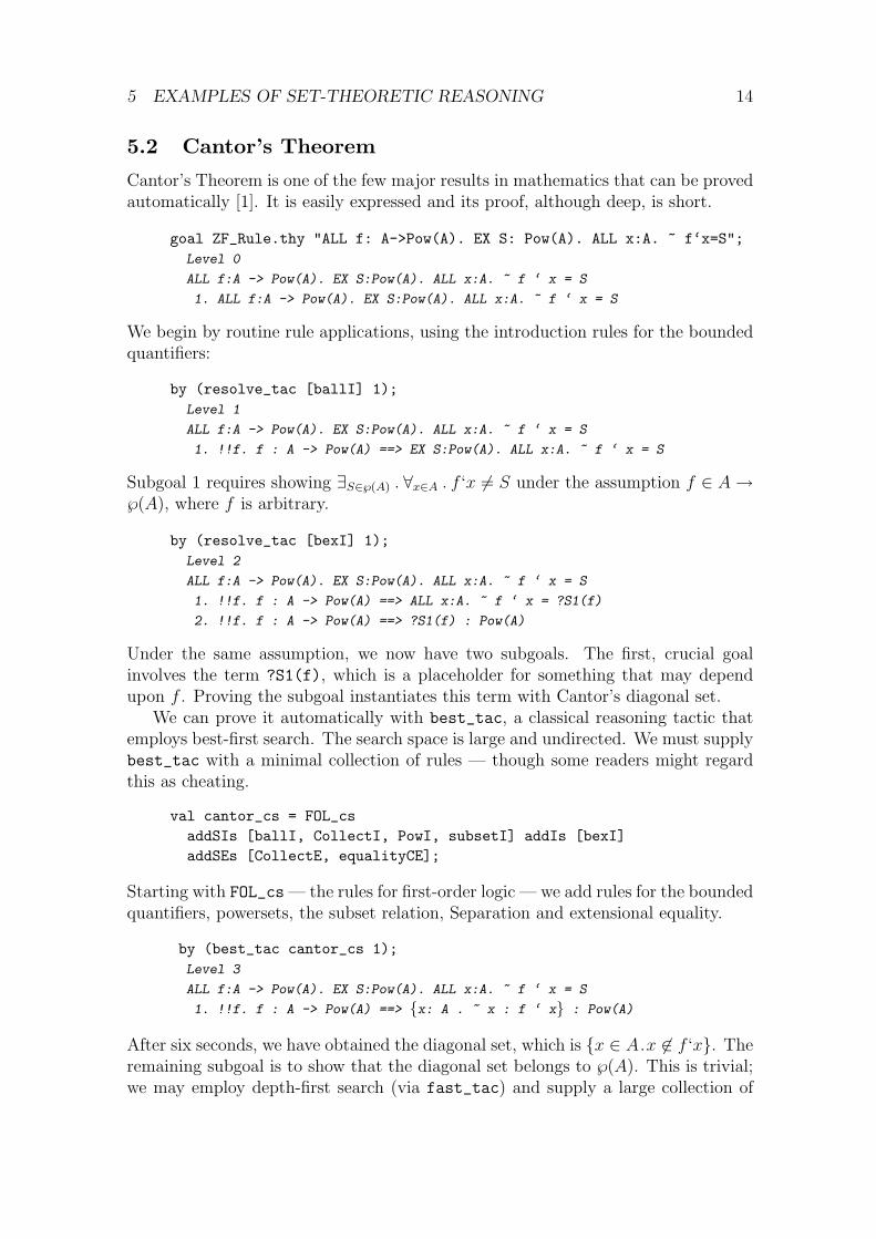
5.2 Cantor’s Theorem
Cantor’s Theorem is one of the few major results in mathematics that can be provedautomatically [1]. It is easily expressed and its proof, although deep, is short.
goal ZF_Rule.thy "ALL f: A->Pow(A). EX S: Pow(A). ALL x:A. ~ f‘x=S";Level 0
ALL f:A -> Pow(A). EX S:Pow(A). ALL x:A. ~ f ‘ x = S
1. ALL f:A -> Pow(A). EX S:Pow(A). ALL x:A. ~ f ‘ x = S
We begin by routine rule applications, using the introduction rules for the boundedquantifiers:
by (resolve_tac [ballI] 1);Level 1
ALL f:A -> Pow(A). EX S:Pow(A). ALL x:A. ~ f ‘ x = S
1. !!f. f : A -> Pow(A) ==> EX S:Pow(A). ALL x:A. ~ f ‘ x = S
Subgoal 1 requires showing ∃S∈℘(A) . ∀x∈A . f ‘x 6= S under the assumption f ∈ A→℘(A), where f is arbitrary.
by (resolve_tac [bexI] 1);Level 2
ALL f:A -> Pow(A). EX S:Pow(A). ALL x:A. ~ f ‘ x = S
1. !!f. f : A -> Pow(A) ==> ALL x:A. ~ f ‘ x = ?S1(f)
2. !!f. f : A -> Pow(A) ==> ?S1(f) : Pow(A)
Under the same assumption, we now have two subgoals. The first, crucial goalinvolves the term ?S1(f), which is a placeholder for something that may dependupon f . Proving the subgoal instantiates this term with Cantor’s diagonal set.
We can prove it automatically with best_tac, a classical reasoning tactic thatemploys best-first search. The search space is large and undirected. We must supplybest_tac with a minimal collection of rules — though some readers might regardthis as cheating.
Starting with FOL_cs — the rules for first-order logic — we add rules for the boundedquantifiers, powersets, the subset relation, Separation and extensional equality.
by (best_tac cantor_cs 1);Level 3
ALL f:A -> Pow(A). EX S:Pow(A). ALL x:A. ~ f ‘ x = S
1. !!f. f : A -> Pow(A) ==> {x: A . ~ x : f ‘ x} : Pow(A)
After six seconds, we have obtained the diagonal set, which is {x ∈ A.x 6∈ f ‘x}. Theremaining subgoal is to show that the diagonal set belongs to ℘(A). This is trivial;we may employ depth-first search (via fast_tac) and supply a large collection of
5 EXAMPLES OF SET-THEORETIC REASONING 15
rules (ZF_cs):
by (fast_tac ZF_cs 1);Level 4
ALL f:A -> Pow(A). EX S:Pow(A). ALL x:A. ~ f ‘ x = S
No subgoals!
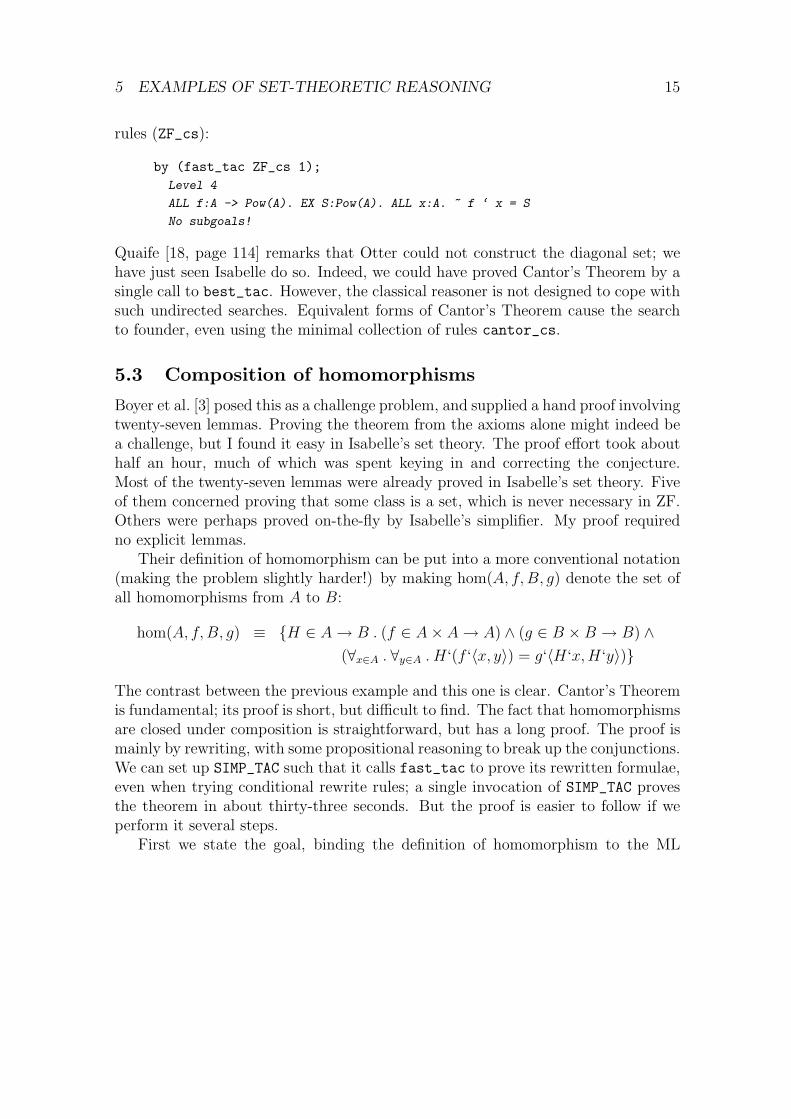
Quaife [18, page 114] remarks that Otter could not construct the diagonal set; wehave just seen Isabelle do so. Indeed, we could have proved Cantor’s Theorem by asingle call to best_tac. However, the classical reasoner is not designed to cope withsuch undirected searches. Equivalent forms of Cantor’s Theorem cause the searchto founder, even using the minimal collection of rules cantor_cs.
5.3 Composition of homomorphisms
Boyer et al. [3] posed this as a challenge problem, and supplied a hand proof involvingtwenty-seven lemmas. Proving the theorem from the axioms alone might indeed bea challenge, but I found it easy in Isabelle’s set theory. The proof effort took abouthalf an hour, much of which was spent keying in and correcting the conjecture.Most of the twenty-seven lemmas were already proved in Isabelle’s set theory. Fiveof them concerned proving that some class is a set, which is never necessary in ZF.Others were perhaps proved on-the-fly by Isabelle’s simplifier. My proof requiredno explicit lemmas.
Their definition of homomorphism can be put into a more conventional notation(making the problem slightly harder!) by making hom(A, f,B, g) denote the set ofall homomorphisms from A to B:
hom(A, f,B, g) ≡ {H ∈ A→ B . (f ∈ A× A→ A) ∧ (g ∈ B ×B → B) ∧(∀x∈A . ∀y∈A . H‘(f ‘〈x, y〉) = g‘〈H‘x,H‘y〉)}
The contrast between the previous example and this one is clear. Cantor’s Theoremis fundamental; its proof is short, but difficult to find. The fact that homomorphismsare closed under composition is straightforward, but has a long proof. The proof ismainly by rewriting, with some propositional reasoning to break up the conjunctions.We can set up SIMP_TAC such that it calls fast_tac to prove its rewritten formulae,even when trying conditional rewrite rules; a single invocation of SIMP_TAC provesthe theorem in about thirty-three seconds. But the proof is easier to follow if weperform it several steps.
First we state the goal, binding the definition of homomorphism to the ML
5 EXAMPLES OF SET-THEORETIC REASONING 16
identifier hom_def:
val [hom_def] = goal Perm.thy"(!! A f B g. hom(A,f,B,g) == \
J : hom(A,f,B,g) & K : hom(B,g,C,h) --> K O J : hom(A,f,C,h)
1. J : hom(A,f,B,g) & K : hom(B,g,C,h) --> K O J : hom(A,f,C,h)
Next, we expand hom_def in the subgoal:
by (rewtac hom_def);Level 1
J : hom(A,f,B,g) & K : hom(B,g,C,h) --> K O J : hom(A,f,C,h)
1. J :
{H: A -> B .
f : A * A -> A &
g : B * B -> B &
(ALL x:A. ALL y:A. H ‘ (f ‘ <x,y>) = g ‘ <H ‘ x,H ‘ y>)} &
K :
{H: B -> C .
g : B * B -> B &
h : C * C -> C &
(ALL x:B. ALL y:B. H ‘ (g ‘ <x,y>) = h ‘ <H ‘ x,H ‘ y>)} -->
K O J :
{H: A -> C .
f : A * A -> A &
h : C * C -> C &
(ALL x:A. ALL y:A. H ‘ (f ‘ <x,y>) = h ‘ <H ‘ x,H ‘ y>)}
Next we invoke a simple tactic from the classical reasoner, in order to break up
5 EXAMPLES OF SET-THEORETIC REASONING 17
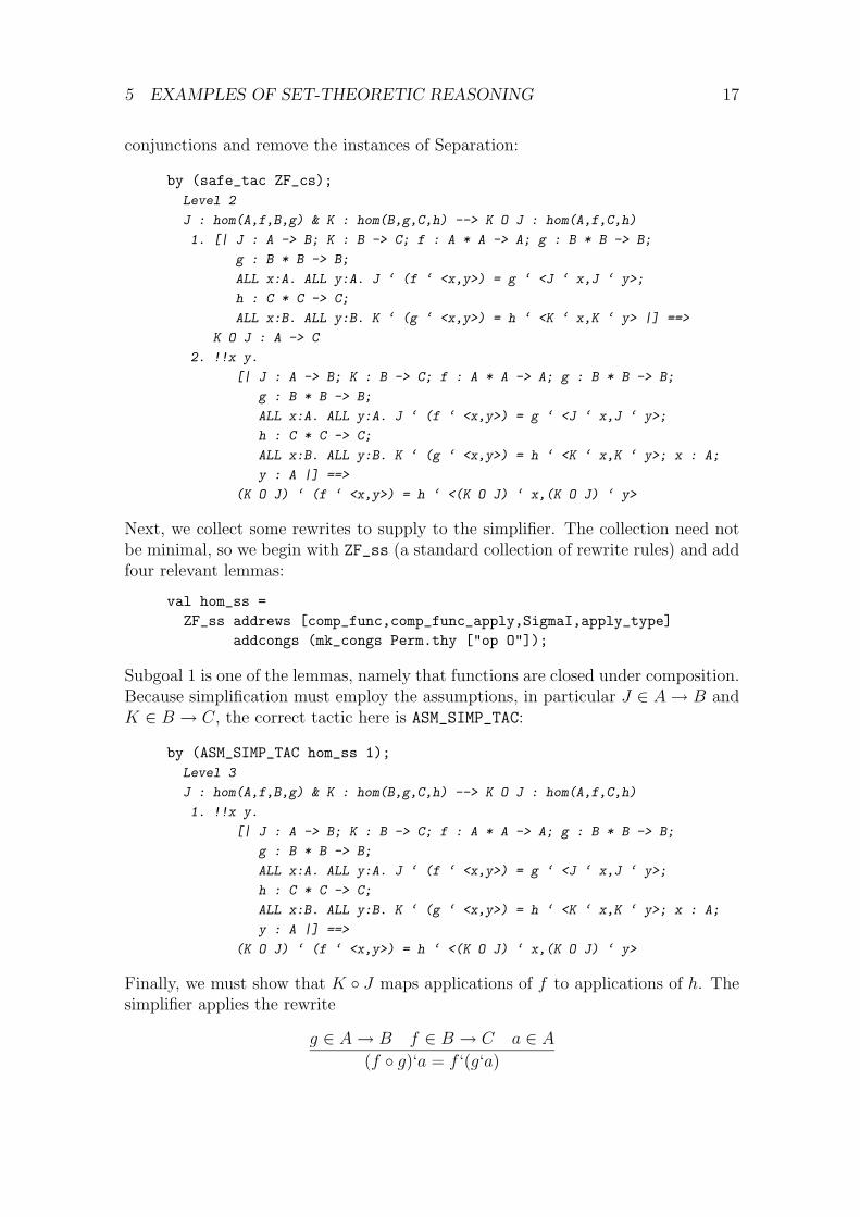
conjunctions and remove the instances of Separation:
by (safe_tac ZF_cs);Level 2
J : hom(A,f,B,g) & K : hom(B,g,C,h) --> K O J : hom(A,f,C,h)
1. [| J : A -> B; K : B -> C; f : A * A -> A; g : B * B -> B;
g : B * B -> B;
ALL x:A. ALL y:A. J ‘ (f ‘ <x,y>) = g ‘ <J ‘ x,J ‘ y>;
h : C * C -> C;
ALL x:B. ALL y:B. K ‘ (g ‘ <x,y>) = h ‘ <K ‘ x,K ‘ y> |] ==>
K O J : A -> C
2. !!x y.
[| J : A -> B; K : B -> C; f : A * A -> A; g : B * B -> B;
g : B * B -> B;
ALL x:A. ALL y:A. J ‘ (f ‘ <x,y>) = g ‘ <J ‘ x,J ‘ y>;
h : C * C -> C;
ALL x:B. ALL y:B. K ‘ (g ‘ <x,y>) = h ‘ <K ‘ x,K ‘ y>; x : A;
y : A |] ==>
(K O J) ‘ (f ‘ <x,y>) = h ‘ <(K O J) ‘ x,(K O J) ‘ y>
Next, we collect some rewrites to supply to the simplifier. The collection need notbe minimal, so we begin with ZF_ss (a standard collection of rewrite rules) and addfour relevant lemmas:
val hom_ss =ZF_ss addrews [comp_func,comp_func_apply,SigmaI,apply_type]
addcongs (mk_congs Perm.thy ["op O"]);
Subgoal 1 is one of the lemmas, namely that functions are closed under composition.Because simplification must employ the assumptions, in particular J ∈ A→ B andK ∈ B → C, the correct tactic here is ASM_SIMP_TAC:
by (ASM_SIMP_TAC hom_ss 1);Level 3
J : hom(A,f,B,g) & K : hom(B,g,C,h) --> K O J : hom(A,f,C,h)
1. !!x y.
[| J : A -> B; K : B -> C; f : A * A -> A; g : B * B -> B;
g : B * B -> B;
ALL x:A. ALL y:A. J ‘ (f ‘ <x,y>) = g ‘ <J ‘ x,J ‘ y>;
h : C * C -> C;
ALL x:B. ALL y:B. K ‘ (g ‘ <x,y>) = h ‘ <K ‘ x,K ‘ y>; x : A;
y : A |] ==>
(K O J) ‘ (f ‘ <x,y>) = h ‘ <(K O J) ‘ x,(K O J) ‘ y>
Finally, we must show that K ◦ J maps applications of f to applications of h. Thesimplifier applies the rewrite
g ∈ A→ B f ∈ B → C a ∈ A(f ◦ g)‘a = f ‘(g‘a)
6 RAMSEY’S THEOREM IN ZF 18
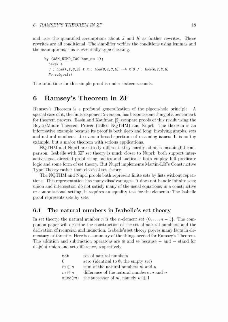
and uses the quantified assumptions about J and K as further rewrites. Theserewrites are all conditional. The simplifier verifies the conditions using lemmas andthe assumptions; this is essentially type checking.
by (ASM_SIMP_TAC hom_ss 1);Level 4
J : hom(A,f,B,g) & K : hom(B,g,C,h) --> K O J : hom(A,f,C,h)
No subgoals!
The total time for this simple proof is under sixteen seconds.
6 Ramsey’s Theorem in ZF
Ramsey’s Theorem is a profound generalization of the pigeon-hole principle. Aspecial case of it, the finite exponent 2 version, has become something of a benchmarkfor theorem provers. Basin and Kaufman [2] compare proofs of this result using theBoyer/Moore Theorem Prover (called NQTHM) and Nuprl. The theorem is aninformative example because its proof is both deep and long, involving graphs, setsand natural numbers. It covers a broad spectrum of reasoning issues. It is no toyexample, but a major theorem with serious applications.
NQTHM and Nuprl are utterly different; they hardly admit a meaningful com-parison. Isabelle with ZF set theory is much closer to Nuprl: both support inter-active, goal-directed proof using tactics and tacticals; both employ full predicatelogic and some form of set theory. But Nuprl implements Martin-Lof’s ConstructiveType Theory rather than classical set theory.
The NQTHM and Nuprl proofs both represent finite sets by lists without repeti-tions. This representation has many disadvantages: it does not handle infinite sets;union and intersection do not satisfy many of the usual equations; in a constructiveor computational setting, it requires an equality test for the elements. The Isabelleproof represents sets by sets.
6.1 The natural numbers in Isabelle’s set theory
In set theory, the natural number n is the n-element set {0, . . . , n − 1}. The com-panion paper will describe the construction of the set of natural numbers, and thederivation of recursion and induction. Isabelle’s set theory proves many facts in ele-mentary arithmetic. Here is a summary of the things needed for Ramsey’s Theorem.The addition and subtraction operators are ⊕ and ª because + and − stand fordisjoint union and set difference, respectively.
nat set of natural numbers0 zero (identical to ∅, the empty set)m⊕ n sum of the natural numbers m and nmª n difference of the natural numbers m and nsucc(m) the successor of m, namely m⊕ 1
6 RAMSEY’S THEOREM IN ZF 19
6.2 The definitions in ZF
Rather than attempt to improve Basin and Kaufmann’s description of Ramsey’sTheorem, I briefly discuss the corresponding definitions. I have used these largelyas abbreviations, rather than as abstract notions; in most of the Isabelle proofs, thedefinitions are expanded.
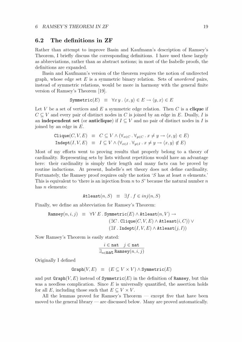
Basin and Kaufmann’s version of the theorem requires the notion of undirectedgraph, whose edge set E is a symmetric binary relation. Sets of unordered pairs,instead of symmetric relations, would be more in harmony with the general finiteversion of Ramsey’s Theorem [19].
Symmetric(E) ≡ ∀x y . 〈x, y〉 ∈ E → 〈y, x〉 ∈ ELet V be a set of vertices and E a symmetric edge relation. Then C is a clique ifC ⊆ V and every pair of distinct nodes in C is joined by an edge in E. Dually, I isan independent set (or anticlique) if I ⊆ V and no pair of distinct nodes in I isjoined by an edge in E.
Clique(C, V,E) ≡ C ⊆ V ∧ (∀x∈C . ∀y∈C . x 6= y → 〈x, y〉 ∈ E)
Indept(I, V, E) ≡ I ⊆ V ∧ (∀x∈I . ∀y∈I . x 6= y → 〈x, y〉 6∈ E)
Most of my efforts went to proving results that properly belong to a theory ofcardinality. Representing sets by lists without repetitions would have an advantagehere: their cardinality is simply their length and many facts can be proved byroutine inductions. At present, Isabelle’s set theory does not define cardinality.Fortunately, the Ramsey proof requires only the notion ‘S has at least n elements.’This is equivalent to ‘there is an injection from n to S’ because the natural number nhas n elements:
Atleast(n, S) ≡ ∃f . f ∈ inj(n, S)
Finally, we define an abbreviation for Ramsey’s Theorem:
Ramsey(n, i, j) ≡ ∀V E . Symmetric(E) ∧ Atleast(n, V )→(∃C . Clique(C, V,E) ∧ Atleast(i, C)) ∨(∃I . Indept(I, V, E) ∧ Atleast(j, I))
Now Ramsey’s Theorem is easily stated:
i ∈ nat j ∈ nat
∃n∈nat Ramsey(n, i, j)
Originally I defined
Graph(V,E) ≡ (E ⊆ V × V ) ∧ Symmetric(E)
and put Graph(V,E) instead of Symmetric(E) in the definition of Ramsey, but thiswas a needless complication. Since E is universally quantified, the assertion holdsfor all E, including those such that E ⊆ V × V .
All the lemmas proved for Ramsey’s Theorem — except five that have beenmoved to the general library — are discussed below. Many are proved automatically.
6 RAMSEY’S THEOREM IN ZF 20
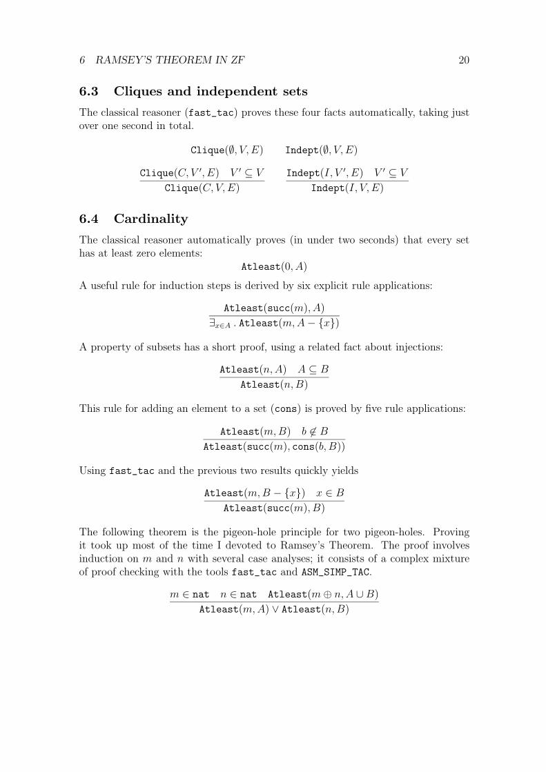
6.3 Cliques and independent sets
The classical reasoner (fast_tac) proves these four facts automatically, taking justover one second in total.
Clique(∅, V, E) Indept(∅, V, E)
Clique(C, V ′, E) V ′ ⊆ V
Clique(C, V,E)
Indept(I, V ′, E) V ′ ⊆ V
Indept(I, V, E)
6.4 Cardinality
The classical reasoner automatically proves (in under two seconds) that every sethas at least zero elements:
Atleast(0, A)
A useful rule for induction steps is derived by six explicit rule applications:
Atleast(succ(m), A)
∃x∈A . Atleast(m,A− {x})
A property of subsets has a short proof, using a related fact about injections:
Atleast(n,A) A ⊆ B
Atleast(n,B)
This rule for adding an element to a set (cons) is proved by five rule applications:
Atleast(m,B) b 6∈ BAtleast(succ(m), cons(b, B))
Using fast_tac and the previous two results quickly yields
Atleast(m,B − {x}) x ∈ BAtleast(succ(m), B)
The following theorem is the pigeon-hole principle for two pigeon-holes. Provingit took up most of the time I devoted to Ramsey’s Theorem. The proof involvesinduction on m and n with several case analyses; it consists of a complex mixtureof proof checking with the tools fast_tac and ASM_SIMP_TAC.
m ∈ nat n ∈ nat Atleast(m⊕ n,A ∪B)
Atleast(m,A) ∨ Atleast(n,B)
6 RAMSEY’S THEOREM IN ZF 21
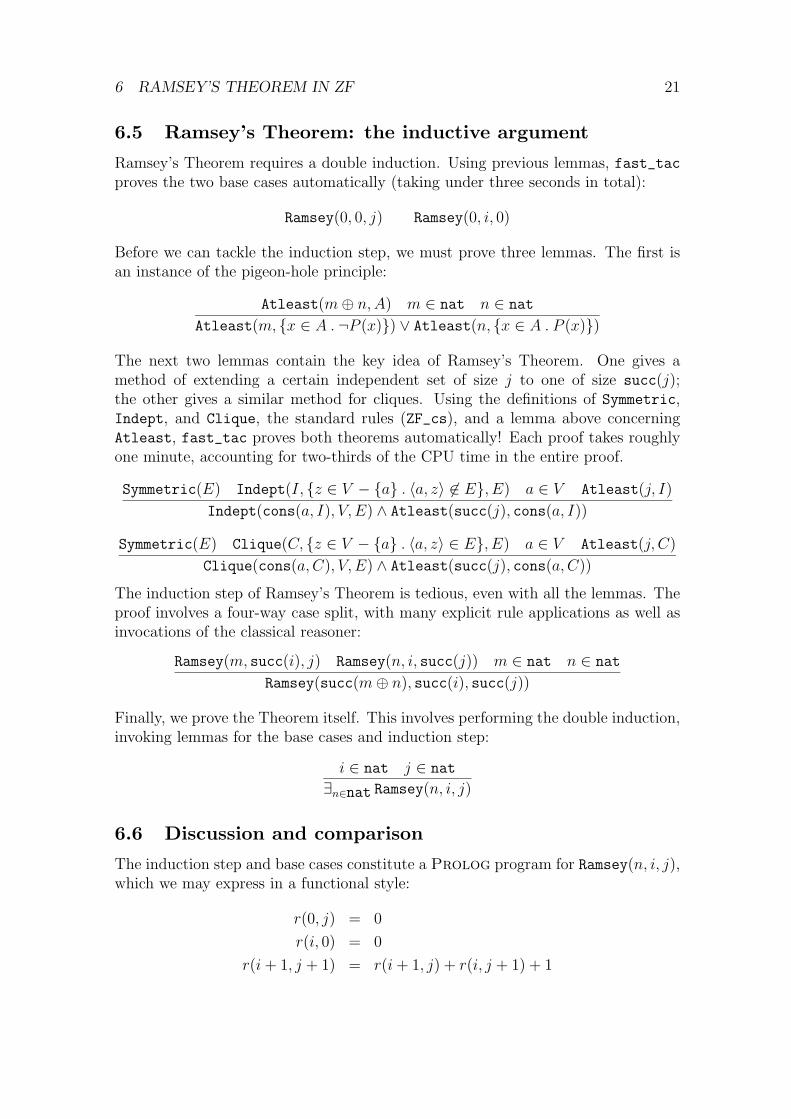
6.5 Ramsey’s Theorem: the inductive argument
Ramsey’s Theorem requires a double induction. Using previous lemmas, fast_tacproves the two base cases automatically (taking under three seconds in total):
Ramsey(0, 0, j) Ramsey(0, i, 0)
Before we can tackle the induction step, we must prove three lemmas. The first isan instance of the pigeon-hole principle:
Atleast(m⊕ n,A) m ∈ nat n ∈ nat
Atleast(m, {x ∈ A . ¬P (x)}) ∨ Atleast(n, {x ∈ A . P (x)})
The next two lemmas contain the key idea of Ramsey’s Theorem. One gives amethod of extending a certain independent set of size j to one of size succ(j);the other gives a similar method for cliques. Using the definitions of Symmetric,Indept, and Clique, the standard rules (ZF_cs), and a lemma above concerningAtleast, fast_tac proves both theorems automatically! Each proof takes roughlyone minute, accounting for two-thirds of the CPU time in the entire proof.
Symmetric(E) Indept(I, {z ∈ V − {a} . 〈a, z〉 6∈ E}, E) a ∈ V Atleast(j, I)
The induction step of Ramsey’s Theorem is tedious, even with all the lemmas. Theproof involves a four-way case split, with many explicit rule applications as well asinvocations of the classical reasoner:
Ramsey(m, succ(i), j) Ramsey(n, i, succ(j)) m ∈ nat n ∈ nat
Ramsey(succ(m⊕ n), succ(i), succ(j))
Finally, we prove the Theorem itself. This involves performing the double induction,invoking lemmas for the base cases and induction step:
i ∈ nat j ∈ nat
∃n∈nat Ramsey(n, i, j)
6.6 Discussion and comparison
The induction step and base cases constitute a Prolog program for Ramsey(n, i, j),which we may express in a functional style:
r(0, j) = 0
r(i, 0) = 0
r(i+ 1, j + 1) = r(i+ 1, j) + r(i, j + 1) + 1
6 RAMSEY’S THEOREM IN ZF 22
Since r(i, j) computes a number n satisfying Ramsey(n, i, j), it is called the wit-nessing function for Ramsey’s Theorem. Basin and Kaufman [2] obtain slightlydifferent Ramsey numbers; the definitions reflect details of the proofs.
Nuprl expresses Ramsey’s Theorem using quantifiers, as here. Since its logicis constructive, Nuprl can extract a witnessing function from the proof. NQTHMlacks quantifiers; it expresses Ramsey’s Theorem in terms of a witnessing function,obtained from a hand proof. Both the Nuprl and NQTHM proofs involve additionalwitnessing functions, which map a graph of sufficient size to a clique or independentset. The Isabelle proof follows the same reasoning as Basin and Kaufman’s proofs; itdoes not make essential use of classical logic. Because it is conducted in classical ZFset theory, there is no way of extracting such witnessing functions from the proof.
The table compares the NQTHM, Nuprl and Isabelle/ZF proofs:
The figures for Isabelle include all the definitions and lemmas given above, and theirproofs. The Isabelle proof has the fewest definitions and lemmas. But NQTHM hasby far the shortest replay time, since a Sun SPARCstation ELC is three or four timesfaster than a Sun 3/60. Kaufman took seven hours to find the NQTHM proof; Basinrequired twenty hours, plus a further sixty for library development [2]. I took aboutnine hours to develop the Isabelle proof, including all lemmas.
Tokens were counted, after removal of comments, by the Unix command
sed -e "s/[^A-Za-z0-9’_]/ /g" ramsey.ML | wc
This counts identifiers but not symbols such as : and =, and is therefore an un-derestimate. It counts seven tokens in EX x:A. Atleast(m, A-{x}). Basin andKaufman each used different methods for counting tokens in their proofs. Figure 1gives a more pessimistic impression of the token density of Isabelle proofs. Onetheorem is proved automatically. Another, which is the main induction step, hasthe second longest proof of the entire effort. The third is Ramsey’s Theorem itself,with its inductions on i and j.
Comparisons are difficult. There are discrepancies in the hardware, token count-ing methods, etc. Furthermore, each author of a proof was an expert with hissystem. We can hardly predict how the systems would compare if tested by novices.The proof requires familiarity with both the system and its library of theorems.
Given these reservations, what conclusions can we draw? Isabelle stands up wellagainst two extensively developed systems, despite its lack of arithmetic decisionprocedures and small size (about 9000 lines of Standard ML, excluding object-logicdefinitions). More importantly, the ZF proof demolishes the myth that axiomaticset theory is too cumbersome to use. Its formal language can be made clear and
Figure 1: Part of the Isabelle proof of Ramsey’s Theorem
7 PREVIOUS WORK USING ISABELLE 24
natural, and Isabelle’s tools — though far from perfect — allow proofs to proceedin large steps.
7 Previous work using Isabelle
Isabelle has supported some form of ZF set theory since its early days. My originalversion consisted of idiosyncratic axioms over the classical sequent calculus LK, withderived sequent rules for the set constructors [13, page 382].
When Philippe Noel started working in set theory, he found both the axiomsand the sequent calculus uncongenial. He adopted Suppes’s axioms and naturaldeduction (then newly available). Isabelle’s set theory was developed only up toordered pairs. Noel went on to prove a large body of results: theorems aboutrelations, functions, orderings, fixed points, recursion, and more [10].
His priority was to develop as much mathematics as possible, not to create shortand elegant proofs. Many of his proofs comprised ten, fifty or even 100 tactic steps.Tactical proofs are a form of software; the simpler they are, the easier they are tounderstand and maintain. Martin Coen adopted some of Noel’s proofs for his ownuse [5]. He polished them a bit, but much more remained to be done.
The present work is an attempt to make set theory easy. Simple facts shouldhave simple proofs: a few rule applications or tool invocations. This has largely beenaccomplished; proofs are easily an order of magnitude simpler than before. Here aresome techniques for taming set theory.
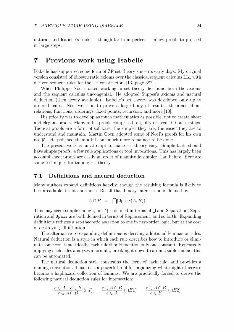
7.1 Definitions and natural deduction
Many authors expand definitions heavily, though the resulting formula is likely tobe unreadable, if not enormous. Recall that binary intersection is defined by
A ∩B ≡⋂
(Upair(A,B)).
This may seem simple enough, but⋂
is defined in terms of⋃
and Separation; Sepa-ration and Upair are both defined in terms of Replacement, and so forth. Expandingdefinitions reduces a set-theoretic assertion to one in first-order logic, but at the costof destroying all intuition.
The alternative to expanding definitions is deriving additional lemmas or rules.Natural deduction is a style in which each rule describes how to introduce or elimi-nate some constant. Ideally, each rule should mention only one constant. Repeatedlyapplying such rules analyses a formula, breaking it down to atomic subformulae; thiscan be automated.
The natural deduction style constrains the form of each rule, and provides anaming convention. Thus, it is a powerful tool for organizing what might otherwisebecome a haphazard collection of lemmas. We are practically forced to derive thefollowing natural deduction rules for intersection:
c ∈ A c ∈ Bc ∈ A ∩B (∩I) c ∈ A ∩B
c ∈ A (∩E1) c ∈ A ∩Bc ∈ B (∩E2)
7 PREVIOUS WORK USING ISABELLE 25
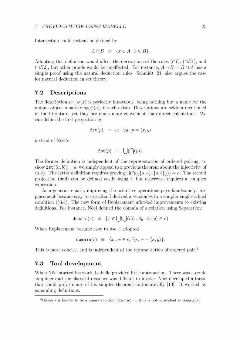
Intersection could instead be defined by
A ∩B ≡ {x ∈ A . x ∈ B}.
Adopting this definition would affect the derivations of the rules (∩I), (∩E1), and(∩E2), but other proofs would be unaffected. For instance, A ∩ B = B ∩ A has asimple proof using the natural deduction rules. Schmidt [21] also argues the casefor natural deduction in set theory.
7.2 Descriptions
The description ιx . ψ(x) is perfectly innocuous, being nothing but a name for theunique object a satisfying ψ(a), if such exists. Descriptions are seldom mentionedin the literature, yet they are much more convenient than direct calculatons. Wecan define the first projection by
fst(p) ≡ ιx . ∃y . p = 〈x, y〉
instead of Noel’s
fst(p) ≡⋃
(⋂
(p)).
The former definition is independent of the representation of ordered pairing; toshow fst(〈a, b〉) = a, we simply appeal to a previous theorem about the injectivity of〈a, b〉. The latter definition requires proving
⋃(⋂
({{a, a}, {a, b}})) = a. The secondprojection (snd) can be defined easily using ι, but otherwise requires a complexexpression.
As a general remark, improving the primitive operations pays handsomely. Re-placement became easy to use after I derived a version with a simpler single-valuedcondition (§3.4). The new form of Replacement afforded improvements to existingdefinitions. For instance, Noel defined the domain of a relation using Separation:
domain(r) ≡ {x ∈⋃
(⋃
(r)) . ∃y . 〈x, y〉 ∈ r}
When Replacement became easy to use, I adopted
domain(r) ≡ {x . w ∈ r, ∃y . w = 〈x, y〉}.
This is more concise, and is independent of the representation of ordered pair.4
7.3 Tool development
When Noel started his work, Isabelle provided little automation. There was a crudesimplifier and the classical reasoner was difficult to invoke. Noel developed a tacticthat could prove many of his simpler theorems automatically [10]. It worked byexpanding definitions.
4Unless r is known to be a binary relation, {fst(w) . w ∈ r} is not equivalent to domain(r).
8 CONCLUSIONS 26
Much later, I modified Isabelle’s classical reasoner to be generic, and suitablefor set theory. To help prevent subgoals of the form t ∈ ?A from causing runawayinstantiations (see §3.1), I reordered the premises of some rules. (Premises createsubgoals, which are normally processed from left to right, like in Prolog.) Finally, Iextended Isabelle with ways of preventing the instantiation of unknowns in subgoals.
Also during this period, Tobias Nipkow installed his simplifier [9].Specialized rewriters and theorem provers may be much faster, but Isabelle’s
tools offer satisfactory performance: they normally return in a few seconds. Becausemy proof style minimizes the expanding of definitions, defining new concepts doesnot make proofs slower.
Tools obviously improve user productivity; moreover, the resulting proofs areresilient. Proof checking causes brittleness: proofs ‘break’ (fail to replay) after theslightest change to a definition or axiom. Tools generally adapt to changes. For astriking example of resilience, recall the pigeon-hole principle:
m ∈ nat n ∈ nat Atleast(m⊕ n,A ∪B)
Atleast(m,A) ∨ Atleast(n,B)
The lemma can be strengthened: replace m⊕ n by m⊕ nª 1, where 1 ≡ succ(0).When I did this, the previous proof (consisting of twenty-eight commands!) replayedperfectly. The nested inductions went precisely as before; the case analyses wereidentical. The · · · ª succ(0) caused no difficulties because all subgoals containingit were submitted to the simplifier, using a general collection of arithmetic rewrites.This was partly luck, but the new version of the pigeon-hole principle required onlyslight changes to the rest of Ramsey’s Theorem.
8 Conclusions
Isabelle’s version of ZF set theory, with its definitions, derived rules and tools, hasreached an advanced sate of development. Problems can be stated in a reasonablyfamiliar notation and approached using high-level steps.
Quaife [18] and Saaltink [20] have also performed extensive proofs in axiomaticset theory. Quaife uses NBG set theory. He has obtained a degree of automationfrom the resolution theorem prover Otter; this requires proving a suitable series oflemmas, sometimes stated in a technical form, and carefully assigning weights andother settings of Otter. Saaltink uses the Eves theorem prover, which has the ZFaxioms built in. His proofs consist of commands to the Eves reducer, which canexpand definitions and perform various simplifications.
I would not attempt an objective comparison with Quaife’s work — the culturegap between Isabelle and Otter is too great. But ZF is much more to my tastethan NBG. Quaife forgoes the notations {x ∈ A . ψ(x)} and ιx . ψ(x), which seemessential for clarity. Saaltink’s work uses ZF and its interactive proof style resemblesIsabelle’s.
Boyer et al. [3] and Quaife mention the possibility of theorem provers settlingfamous open questions such as Goldbach’s Conjecture. This seems unlikely in the
REFERENCES 27
near future, especially since some of these open questions may be independent ofthe axioms of set theory. A more immediate goal is to produce a reasoning tool toassist mathematicians, just as symbolic algebra packages assist engineers. Even thismodest goal requires more research. Set theory by itself does not support mathe-matical abstraction — the set-theoretic definition of group leads to a horrendoussyntax for group theory. This is an area where we can make progress.
Isabelle’s set theory records nearly 700 theorems. We have discussed the formaldevelopment, starting from the ZF axioms, of a calculus of sets, pairs, relations andfunctions. This is the starting point for a computational logic. The next devel-opments concern general principles for defining recursive data types, including thenatural numbers — using, for the first time, the Axiom of Infinity! The companionpaper will discuss recursion in all its forms.
Acknowledgements. Philippe Noel’s version of set theory, modified by MartinCoen, was the starting point of the present theory. Tobias Nipkow made greatcontributions to Isabelle, including the simplifier. David Basin, Matt Kaufman,Brian Monahan and Philippe Noel commented usefully on this work.
References
[1] Peter B. Andrews, Dale A. Miller, Eve L. Cohen, and Frank Pfenning. Au-tomating higher-order logic. In W. W. Bledsoe and D. W. Loveland, editors,Automated Theorem Proving: After 25 Years, pages 169–192. American Math-ematical Society, 1984.
[2] David Basin and Matt Kaufmann. The Boyer-Moore prover and Nuprl: Anexperimental comparison. In Gerard Huet and Gordon Plotkin, editors, LogicalFrameworks, pages 89–119. Cambridge University Press, 1991.
[3] Robert Boyer, Ewing Lusk, William McCune, Ross Overbeek, Mark Stickel,and Lawrence Wos. Set theory in first-order logic: Clauses for Godel’s axioms.Journal of Automated Reasoning, 2:287–327, 1986.
[4] Robert S. Boyer and J Strother Moore. A Computational Logic Handbook.Academic Press, 1988.
[5] Martin Coen. Interactive Program Derivation. PhD thesis, University of Cam-bridge, 1992.
[6] Michael J. C. Gordon. Why higher-order logic is a good formalism for specifyingand verifying hardware. In G. Milne and P. A. Subrahmanyam, editors, FormalAspects of VLSI Design, pages 153–177. North-Holland, 1986.
[7] Michael J. C. Gordon. HOL: A proof generating system for higher-order logic.In Graham Birtwistle and P. A. Subrahmanyam, editors, VLSI Specification,Verification and Synthesis, pages 73–128. Kluwer Academic Publishers, 1988.
REFERENCES 28
[8] Paul R. Halmos. Naive Set Theory. Van Nostrand, 1960.
[10] Philippe Noel. Experimenting with Isabelle in ZF set theory. Journal of Auto-mated Reasoning. In press.
[11] Bengt Nordstrom, Kent Petersson, and Jan Smith. Programming in Martin-Lof’s Type Theory. An Introduction. Oxford, 1990.
[12] Lawrence C. Paulson. The foundation of a generic theorem prover. Journal ofAutomated Reasoning, 5:363–397, 1989.
[13] Lawrence C. Paulson. Isabelle: The next 700 theorem provers. In P. Odifreddi,editor, Logic and Computer Science, pages 361–386. Academic Press, 1990.
[14] Lawrence C. Paulson. Introduction to Isabelle. Technical report, University ofCambridge Computer Laboratory, 1992.
[15] Lawrence C. Paulson. The Isabelle reference manual. Technical report, Univer-sity of Cambridge Computer Laboratory, 1992.
[16] Lawrence C. Paulson. Isabelle’s object-logics. Technical report, University ofCambridge Computer Laboratory, 1992.
[17] F. J. Pelletier. Seventy-five problems for testing automatic theorem provers.Journal of Automated Reasoning, 2:191–216, 1986. Errata, JAR 4 (1988), 235–236.
[18] Art Quaife. Automated deduction in von Neumann-Bernays-Godel set theory.Journal of Automated Reasoning, 8(1):91–147, 1992.
[19] Herbert John Ryser. Combinatorial Mathematics. Mathematical Associationof America, 1963.
[20] Mark Saaltink. The EVES library models. Technical Report TR-91-5449-04,ORA Canada, 265 Carling Avanue, Suite 506, Ottawa, Ontario, 1992.
[21] David Schmidt. Natural deduction theorem proving in set theory. Technical Re-port CSR-142-83, Department of Computer Science, University of Edinburgh,1983.
[22] Patrick Suppes. Axiomatic Set Theory. Dover, 1972.