Seth Temple [email protected]Notes STAT 580s 2020-2021 These notes are from courses taught by University of Washington Professors Alex Luedtke and Marco Carone, as well as based on van der Vaart’s Asymptotic Statistics and Wainwright’s High-Dimensional Statistics. Another textbook Weak Convergence and Empirical Processes by van der Vaart and Wellner is used. This book may be abbreviated vdV&W (1996) whereas the blue book may be abbreviated vdV (2000). My contribution is to reword and reorganize course content and to provide some supplementary material. Enjoy the cover page matter and the rest! 1
These notes are from courses taught by University of Washington Professors Alex Luedtke andMarco Carone, as well as based on van der Vaart’s Asymptotic Statistics and Wainwright’sHigh-Dimensional Statistics. Another textbook Weak Convergence and Empirical Processesby van der Vaart and Wellner is used. This book may be abbreviated vdV&W (1996) whereasthe blue book may be abbreviated vdV (2000). My contribution is to reword and reorganizecourse content and to provide some supplementary material. Enjoy the cover page matterand the rest!
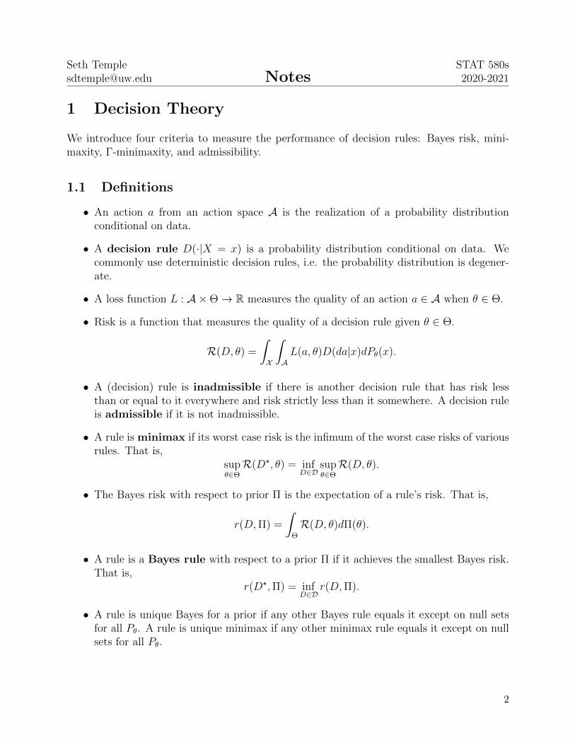
We introduce four criteria to measure the performance of decision rules: Bayes risk, mini-maxity, Γ-minimaxity, and admissibility.
1.1 Definitions
• An action a from an action space A is the realization of a probability distributionconditional on data.
• A decision rule D(·|X = x) is a probability distribution conditional on data. Wecommonly use deterministic decision rules, i.e. the probability distribution is degener-ate.
• A loss function L : A×Θ→ R measures the quality of an action a ∈ A when θ ∈ Θ.
• Risk is a function that measures the quality of a decision rule given θ ∈ Θ.
R(D, θ) =
∫X
∫AL(a, θ)D(da|x)dPθ(x).
• A (decision) rule is inadmissible if there is another decision rule that has risk lessthan or equal to it everywhere and risk strictly less than it somewhere. A decision ruleis admissible if it is not inadmissible.
• A rule is minimax if its worst case risk is the infimum of the worst case risks of variousrules. That is,
supθ∈ΘR(D?, θ) = inf
D∈Dsupθ∈ΘR(D, θ).
• The Bayes risk with respect to prior Π is the expectation of a rule’s risk. That is,
r(D,Π) =
∫Θ
R(D, θ)dΠ(θ).
• A rule is a Bayes rule with respect to a prior Π if it achieves the smallest Bayes risk.That is,
r(D?,Π) = infD∈D
r(D,Π).
• A rule is unique Bayes for a prior if any other Bayes rule equals it except on null setsfor all Pθ. A rule is unique minimax if any other minimax rule equals it except on nullsets for all Pθ.
• An estimator D? is Γ-minimax w.r.t. a loss function if
supΠ∈Γ
r(D?,Π) = infT
supΠ∈Γ
r(T,Π).
This definition is analogous to minimax but w.r.t. Bayes risk as opposed to risk.
• The kernel of a posterior distribution is the function depending on the parameter, notthe proportionality constant. The kernel uniquely determines the posterior distribution.
• A conjugate prior is one such that the posterior distribution is in the same family asthe prior distribution.
• A prior is least favorable if the Bayes risk for the Bayes rule and the prior achievesthe supremum over priors of Bayes risks for paired Bayes rules and priors.
• A sequence of priors is least favorable if, for all priors Π,
r(DΠ,Π) ≤ lim infk→∞
r(DΠk ,Πk).
1.2 Results
• Finding Bayes rules by minimizing the conditional expected loss. Supposethat θ ∼ Π, X|θ = θ ∼ Pθ, and the loss is nonnegative. If,
(i) there is a rule with finite Bayes risk, and
(ii) there exists DΠ ∈ D for almost all x that minimizes the conditional expected loss,
then DΠ is a Bayes rule.
• If the loss function is convex for fixed θ, decision rules are unrestricted, the action spaceis convex, and there is a Bayes rule, then there is a deterministic Bayes rule.
• Constant risk theorem. If Π satisfies
r(DΠ,Π) = supθ∈ΘR(DΠ, θ),
then (i) DΠ is minimax, (ii) unique Bayes DΠ w.r.t. Π implies unique minimax, and(iii) Π is a least favorable prior.
• Constant risk theorem (ii). For a sequence of priors Πk, if D ∈ D satisfies
supθ∈ΘR(D, θ) = lim inf
k→∞r(DΠk ,Πk),
then (i) D is minimax, and (ii) Πk is a least favorable prior sequence.
• Constant Bayes risk theorem. If Π? ∈ Γ satisfies
r(DΠ? ,Π?) = supΠ∈Γ
r(DΠ? ,Π)
then (i) DΠ? is Γ-minimax, (ii) unique Bayes DΠ? implies unique minimax, and (iii) Π?
is a least favorable prior.
• If a minimax estimator for a smaller model has no worse worst-case risk scenario for alarge model, then the estimator is minimax for the larger model as well. (See slide 36.)
• Some admissible estimators. (i) Any unique Bayes rule is admissible, and (ii) anyunique minimax rule is admissible. Moreover, for squared error loss, finite r(DΠ,Π),and
∫Pθ(X ∈ A)dΠ(θ) = 0 implying Pθ(X ∈ A) = 0 for all θ, we have that DΠ is a
unique Bayes rule.
• Stein’s lemma. Let Y ∼ N(µ, σ2) and let g : R → R be such that E[|g′(Y )|] < ∞.Then, E[g(Y )(Y − µ)] = σ2E[g′(Y )]. (See slides 74-76 for multivariate generalization.)
1.3 Examples
• The posterior mean is the (deterministic) Bayes rule under L2 loss.
• The posterior median is the (deterministic) Bayes rule under L1 loss.
• The posterior mode is the (deterministic) Bayes rule under 0-1 loss.
• The sample mean is a minimax estimator for θ in an X ≡ (X1, · · · , Xn) iid sample ofN(θ, σ2) random variables.
• The sample mean is an admissible estimator for θ in the case of univariate normalswith mean θ. The sample mean is inadmissible for dimension three or higher.
• The James-Stein estimator beats the sample mean when estimating a mean vector ofdimension 3 or more. The positive-part James-Stein estimator beats the James-Steinestimator, so the James-Stein estimator is inadmissible too. Intuitively, the James-Steinestimator shrinks the sample mean towards zero (or some other point).
T JS(x) =
(1− (d−2)σ2
n||xn||2 )xn xn 6= (0, · · · , 0)
0 otherwise.
In some cases, we can reduce the James-Stein estimator to lower dimensions by leverag-ing the fact that it is a spherically symmetric estimator, where a spherically symmetricestimator is of the form Tτ (x) = τ(||x||)x. This fact solicits some geometric intuition(see slides 63-72). The shrinkage property creates bias and may be inappropriate for es-timating individual means. Finally, we can motivate these estimators from an empiricalBayes perspective.
These results facilitate statistical inference when samples sizes grow to infinity.
2.1 Definitions
• (convergence almost surely) An →a.s. A if P ( limn→∞||An − A|| = 0) = 1.
• (convergence in probability) An →p A if, for all ε > 0, P (||An − A|| > ε)→ 0.
• Rd-valued random variable An converges in distribution to A if, for all bounded, con-tinuous functions f : Rd → R,
E[f(An)]→ E[f(A)].
This convergence is sometimes referred to as weak convergence or convergence in law.
• Uniform integrability: Xn is u.i. if supn E[|Xn| · 1|Xn| ≥ a] → 0. This is acondition controlling tail probabilities. (Weak convergence and u.i. imply convergenceof means.)
• Order notations.
– xn = O(rn) if lim sup |xn/rn| < ∞. Equivalently, there exists M > 0 such thatI|xn| ≤ M |rn| → 1. In layman’s terms, xn is within some multiplicative con-stant of rn.
– xn = o(rn) if lim sup |xn/rn| = 0. Identically, for all M > 0, I|xn| ≤M |rn| → 1.In layman’s terms, xn changes slower than rn.
– Xn = OP (Rn) if, for all ε > 0, there exists M > 0 s.t.
lim inf P (||Xn|| ≤M ||Rn||) > 1− ε.
– Xn = oP (Rn) if, for all M > 0,
P (||Xn|| ≤M ||Rn||)→ 1.
– Stochastic and determisitic notations are equivalent when Xna.s.= xn and Rn
a.s.= rn.
– Xn = oP (1) if and only if Xn →p 0.
– Xn = OP (1) is also referred to as the random sequence being uniformly tight.
– oP (1) is related to convergence in probability whereas OP (1) is related to weakconvergence.
– Read these useful properties left to right as an implication:
(1) Xn = oP (Rn) if and only if Xn = RnYn for some Yn = oP (1);
(2) Xn = OP (Rn) if and only if Xn = RnYn for some Yn = OP (1);
(3) oP (1) + oP (1) = oP (1);
(4) oP (1) +OP (1) = OP (1);
(5) OP (1)OP (1) = OP (1);
(6) oP (1)OP (1) = oP (1);
(7) [1 + oP (1)]−1 = OP (1);
(8) Xn = oP (1) implies Xn = OP (1).
2.2 Results
• Almost sure convergence implies convergence in probability implies weak convergence.
• Let An, A, and B be defined on a common probability space. An →a.s. A andAn →a.s. B implies A = B almost surely. An →p A and An →p B implies A = B
almost surely. Similarly, if Xn →d X and Xn →d X, then Xd= X. This juxtaposition
highlights that the weak limit X is only unique up to its distribution, whereas the otherconvergence limits are unique.
• Portmanteau theorem. TFAE definitions for weak convergence ⇒. Some of theseinterpretations of weak convergence are more useful than others in proving certainresults. Search this list for the appropriate definition for any proof at hand.
(i) E[f(Xn)]→ E[f(X)] for all bounded, continuous f .
(ii) P (Xn ≤ x)→ P (X ≤ x) for all continuity points x of P (X ≤ ·).(iii) E[f(Xn)]→ E[f(X)] for all bounded, Lipschitz-continuous f .
(iv) lim supE[f(Xn)] ≤ E[f(A)] for every upper semicontinuous f bounded above.
(v) lim inf E[f(Xn)] ≥ E[f(X)] for every lower semicontinuous f bounded below.
(vi) lim supP (Xn ∈ F ) ≤ P (X ∈ F ) for all closed sets F .
(vii) lim inf P (Xn ∈ O) ≥ P (X ∈ O) for all open sets O.
(viii) P (Xn ∈ C)→ P (X ∈ C) for all continuity sets C, i.e. sets C s.t. P (X ∈ ∂C) = 0.
(ix) E[expitTXn]→ E[expitTX] for all vectors t. (Levy continuity)
(x) tTXn ⇒ tTX for all vectors t. (Cramer-Wold)
• Continuous mapping. Let f be continuous at every point of C s.t. P (X ∈ C) = 1.
(ii) Xn ⇒ X and Yn →p c for constant c implies (Xn, Yn)⇒ (X, c).
• Slutsky’s lemma. This result provides a way to combine random vectors and randomvariables in the asymptote. Be careful with random vectors versus random variables inbetween (i) versus (ii) and (iii).
(i) Xn ⇒ X and Yn →p c for multidimensional constant c implies Xn + Yn ⇒ X + c;
(ii) Xn ⇒ X and Yn →p c for 1-dim constant c implies XnYn ⇒ cX;
(iii) Xn ⇒ X and Yn →p c for nonzero 1-dim constant c implies Xn + Yn ⇒ X/c.
• Laws of large numbers. Let E[|X|] <∞. Then,
– (weak law of large numbers) Xn →p E[X];
– (strong law of large numbers) Xn →a.s E[X].
• Prokhorov theorem. This theorem relates to how oP (1) is linked with converge inprobability. Here we see a relationship between OP (1) and weak convergence. Theresult is not quite an if and only if result. (ii) is similar to the Bolzano-Weierstrasstheorem from real analysis.
(i) Xn ⇒ X for some X implies that X = OP (1).
(ii) Xn = OP (1) implies that there is a subsequence Xni s.t. Xni ⇒ X for some X.
• Central limit theorems.
– (vanilla univariate CLT) iid sample and finite second moment implies
– (univariate) If f : Rd → R is differentiable at ψ0 and rn(ψn − ψ0)⇒ Z, then
rn(f(ψn)− f(ψ0))⇒ 〈Z,∇f(ψ0)〉;
– (multivariate) if f : Rd → Rp is differentiable at ψ0 and rn(ψn − ψ0)⇒ Z, then
rn(f(ψn)− f(ψ0))⇒ JfZ,
where Jf is the Jacobian with respect to function f .
2.3 Examples
• Examples
– The vanilla univariate central limit theorem is a special case of the Lindeberg-Fellercentral limit theorem when we have iid samples.
– See slides 40-44 applying Lindeberg-Feller for simple linear regression with a fixeddesign. This example is also discussed in Amy Willis’s BIOST 533. Moreover, wecan find another Lindeberg-Feller example on the BIOST 533 final exam.
– Samples from standard multivariate normals have nice weak convergence results.See Homework 2. The crux is to decompose the random vector into polar coordi-nates and consider generic orthogonal transformations.
– Estimation of relative risk using a delta method. See end of Chapter 2 slides.
• Counterexamples
– Convergence in probability does not imply almost sure convergence. We considera sequence of indicators that splits [0,1] into halves, then thirds, then fourths, andso on. As n gets large, this sequence of random variables converges in probabilityto zero. However, the indicator is triggered infinitely often, so the sequence doesnot converge almost surely to zero.
– Convergence in distribution does not imply convergence in probability. We con-sider a sequence that converges weakly to a symmetric distribution.
– Dependent sequences that marginally converge weakly may not jointly convergeweakly. We consider sequences where the covariance between random variablesalternate between -1 and 1. With independence, marginal weak convergencesimply joint weak convergence.
We introduce two paradigms for deriving estimators for a parameter θ. M for “maximum” inM -estimation involves maximizing a criterion function. Z for “zero” in Z-estimation involvesfinding roots of a criterion function.
3.1 Definitions
• Empirical process notation provides shorthand
Pf ≡∫f(x) dP (x)
Pnf ≡1
n
n∑i
f(Xi)
• If φ0 ≡ φ(θ0) ∈ arg maxφ P0mφ, then φn ∈ arg maxφ Pnmφ is an M -estimator. Moregenerally, we consider M0 and Mn that do not have to be P0mφ and Pnmφ.
• If φ0 is a solution to P0zφ = 0, then the solution φn to Pnzφ = 0 is a Z-estimator. Moregenerally, we consider Z0 and Zn that do not have to be P0zφ and Pnzφ.
• We call mφ : φ ∈ S ⊃ Im(Φ) a P0-GC class if supφ |(Pn − P0)mφ| = oP (1)
• The bracketing number measures how complex the class of functions F is. See slides21-26 for an introduction with application in the Glivenko-Cantelli theorem.
• The root density θ 7→ √pθ is differentiable in quadratic mean at θ if there exists a
pseudoscore function ˙θ such that
sup||h||=1
∫ (√pθ+εh −
√pθ
ε− hT ˙
θ
2
√pθ
)2
dµε→0−→ 0
This definition is akin to differentiability except an integral is thrown into the mix. Itis exactly what we require to weaken the regularity condition of first and second orderdifferentiability for asymptotic normality. We say a model is QMD if its root densityis QMD. The pseudoscore is the score under reasonable conditions.
• The squared Hellinger distance is involved in QMD arguments.
H2(Pε, P0) ≡∫ (√pε −
√p0
)2
dµ
• L2(µ) contains µ-measurable functions f such that∫f 2dµ is finite. This space is
equipped with inner product and norm, so the triangle and reverse triangle inequalitieshold.
• Under conditions for Radon-Nikodym derivatives, the Kullback-Leibler divergence servesas an mφ justifying maximum likelihood estimators as M -estimators.
• Under certain conditions, the M -estimation problem (maximizing) can be expressedas a Z-estimation problem (root-finding). On the other hand, Mθ(φ) = −||Zθ(φ)||expresses a Z-estimation problem as an M -estimation problem.
• Uniform consistency. Suppose that
(i) a near-maximizer for Mn is available: φn satisfies Mn(φn) ≥ supφMn(φ)− oP (1);
(ii) Mn is uniformly consistent: supφ |Mn(φ)−M0(φ)| →p 0; and
(iii) φ0 is well-separated: ∀ε > 0, M0(φ0) > sup||φ−φ0||>εM0(φ).
Then, φn →p φ0.
Finding a maximum is a good way to satisfy (i). In Homework 4 Problem 1(a), weformulate a case where missing condition (iii) results in the conclusion not holding.
• Consistency of Z-estimators in one dimension. Let Im(Φ)⊂ R and, for all φ,Zn(φ)→p Z0(φ). One or the other or both must hold:
(i) φ 7→ Zn(φ) is continuous and has one root φn.
(ii) φ 7→ Zn(φ) is nondecreasing and there is φn such that Zn(φn) = oP (1).
φ0 such that, for all ε > 0, Z0(φ0 − ε) < 0 < Z0(φ0 + ε) implies φn →p φ0.
This result is analogous to Homework 4 Problem 4(b).
• Glivenko-Cantelli theorems.
(i) If F is a class of functions with finite bracketing number for all ε > 0, F is P0-GC:
||Pn − P0||F ≡ supf|(Pn − P0)f | = oP (1).
(ii) Suppose F ≡ fφ : φ ∈ K for K ⊂ Rd compact. If φ(x) 7→ fφ(x) is continuousfor all x and there is an envelope function F satisfying P0F < ∞ for whichsupφ |fφ(x)| ≤ F (x) for all x, then the bracketing number is finite for ε > 0.
• Under regularity conditions, we have asymptotic normality for Z- and M -estimators.Regularity conditions are assumptions required such that we achieve our desired result.See Chapter 3 slides 29-36 and van der Vaart Theorems 5.21 and 5.23. Below we writesome of these regularity conditions for Z−estimation.
First, we compare the Wald, score (Rao), and likelihood ratio tests that all converge indistribution to χ2 under regularity conditions. Second, we consider local alternatives wherein sampling from the alternative we maintain desirable properties for our estimators. SeeChapter 4 slides for the hypothesis testing framework.
4.1 Definitions
• The (randomized) test function φn(X) indicates when we reject the null.
• The power function πn(θ) = Eθ[φn(X)] measures the probability we reject the null.
• The size of the test is supθ0∈Θ0
πn(θ0).
• Q is absolutely continuous w.r.t. P means that P (A) = 0 implies Q(A) = 0.
• Qn is contiguous w.r.t Pn means that Pn(An)→ 0 implies Qn(An)→ 0.
• A local alternative is some θ + h/√n where h describes some (small) perturbation
from the null in an arbitrary direction.
• A regular estimator is an estimator whose sampling distribution is invariant to localperturbations of the data-generating distribution.
4.2 Results
• Wald test. This test rejects the null when the estimate ψ of ψ is far from zero. Thetest statistic Wn ≡ nψTAθψ ⇒ χ2(m) under the null where m is the dimension of thespace ψ lives in. This test can be easy to implement when considering many hypothesesbecause the we only find one MLE.
• Likelihood ratio test. This test rejects the null when the KL divergence is large.The test statistic Ln ≡ 2nPn[`θ − `θ0 ] ⇒ χ2(m). This test better controls the type 1error in small samples.
• Score test. This test rejects the null when the empirical mean of the score is far fromzero. The test statistic Sn ≡ Zn(θ0)I−1
θ0Zn(θ0)⇒ χ2(m). This test is easy to implement
because Θ0 is often a lower-dimensional space.
• The pairwise differences between these three tests converge in probability to zero underthe null hypothesis.
• Le Cam’s First Lemma. This lemma helps us to show and characterize contiguity.TFAE:
(i) Qn is contiguous w.r.t. Pn
(ii) Ln ≡ dQandPn
(Zn)Pn⇒ V along a subsequence implies that E[V ] = 1.
(iii) dPandQn
(Zn)Qn⇒ U along a subsequence implies that P (U > 0) = 1.
• Le Cam’s Third Lemma. This lemma shows us how to use contiguity when studying
alternatives. Suppose that Qn is contiguous w.r.t. Pn and (Tn, Ln)Pn⇒ (T, V ). For all
measurable A ⊂ Rd, let R(A) = E[IA(T )V ]. Then R is a probability measure and
TnQn⇒ R.
• Asymptotic normality of log likelihood ratio. Suppose logLnPn⇒ N(µ, σ2). Then
Qn is contiguous w.r.t. Pn if and only if µ = −σ2/2. This result emphasizes that it cansometimes be useful to consider the weak limit of the log likelihood ratio.
• See van der Vaart Theorem 7.2 and Chapter 4 slides 30-40. With this theorem andLe Cam’s Third Lemma, we derive results for Wald tests under local alternatives andregular estimators.
• We achieve perfect asymptotic power at fixed alternatives. That is, if we collect enoughdata, we will always reject a false null hypothesis.
• Wald statistic under local alternative. We assume the regularity conditions forthe asymptotic normality of the MLE. Then, the Wald statistic Wn has a noncentralχ2(m) weak limit where the noncentrality parameter is hTψAθhψ. Because χ2 randomvariables are stochastically increasing in their noncentrality parameter, the Wald testachieves non-trivial power at local alternatives.
• We skipped the section on relative efficiency. See the final Chapter 4 slides.
• Pointwise asymptotic optimality. Suppose there is an estimator θn for each θ such
that√n(θn − θ)
θ⇒ Qθ. For any θ there exists another estimator θn such that
√n(θn − θ′)
θ′⇒
Qθ′ θ′ 6= θ
δ0 otherwise
That is, we can always construct a dominating estimator sequence. The above is theHodges’ estimator. See graph in Chapter 5 slides and van der Vaart Chapter 8.
• Almost everywhere convolution. Assume a QMD model at every θ with nonsin-
gular information Iθ. Suppose√n(θn− θ)
θ⇒ Qθ for every θ. Then, for almost everyθ, there exists Mθ s.t.
Qθ ≡ Z + ε
where Z ∼ N(0, I−1θ ) and ε ∼Mθ.
• Convolution for regular estimators. Let θn be a regular estimator sequence. Underthe same conditions as the a.e. convolution theorem, for all θ, there exists Mθ suchthat
Qθ ≡ Z + ε
where Z ∼ N(0, I−1θ ) and ε ∼Mθ.
• Anderson’s lemma. This theorem coupled with a convolution theorem shows thatthe MLE is asymptotically optimal, i.e. achieves a lower bound. Let Z ∼ N(0,Σ) andε ∼M be independent. If the loss L is quasiconvex and centrally symmetric, thenE[L(Z)] ≤ E[L(Z + ε)].
In nonparametric settings it is challenging to analytically derive optimal minimax risk. Welook at lower and upper bounds to determine an optimal minimax rate.
6.1 Definitions
• For rule T and model P the maximal risk is supP R(T, P ). The minimax rule hasthe smallest maximal risk. Having small maximal risk means a rule will work wellirrespective of the true P . It can be difficult to derive the maximal risk.
• Let P = Qn restrict us to an iid model and Tn denote allowable decision rules given n.A rule sequence Tn is minimax rate optimal if
lim infn→∞
infT∈Tn supQR(T,Qn)
supQR(Tn, Qn)> 0
Establishing rate optimality involves knowing maximal risk of Tn and minimax risk.This chapter contains methods to get lower bounds on minimax risk.
• The discrepancy d(P1, P2) between models is infa∈AL(a, P1) + L(a, P2).
• The testing affinity ||p1 ∧ p2||1 for models P1, P2 ν is∫min
dP1
dν,dP2
dν
dν
Draw the two density curves on the same plot for further elucidation.
• The total variation distance TV(P1, P2) is supA∈A |P1(A)− P2(A)|.
• Integrated squared error is used as the loss for regression and density problems.
where ` is the greatest integer less than β. So these functions are `-times differentiableand satisfy some Lipschitz condition. Assuming this class is useful in smooth regression.The Lipschitz condition here, Holder continuity, fits into a continuity heuristic.
This method proposes a lower bound on minimax risk as a tradeoff between discrepancyand testing affinity or likewise discrepancy and KL divergence. Using this method yieldsa rate-optimal minimax lower bound for estimating a smooth density at a specific point.
• Fano’s method. For P1, · · · , PN ∈ P ,
infT
supPR(T, P ) ≥ η
2
(1−
log 2 +N−1∑N
j=1 KL(Pj, P )
logN
)≥ η
2
(1− log 2 + maxj 6=k KL(Pj, Pk)
logN
)where P is the uniform mixture and η is the minimum discrepancy. Using this methodyields a rate-optimal minimax lower bound for smooth regression problems.
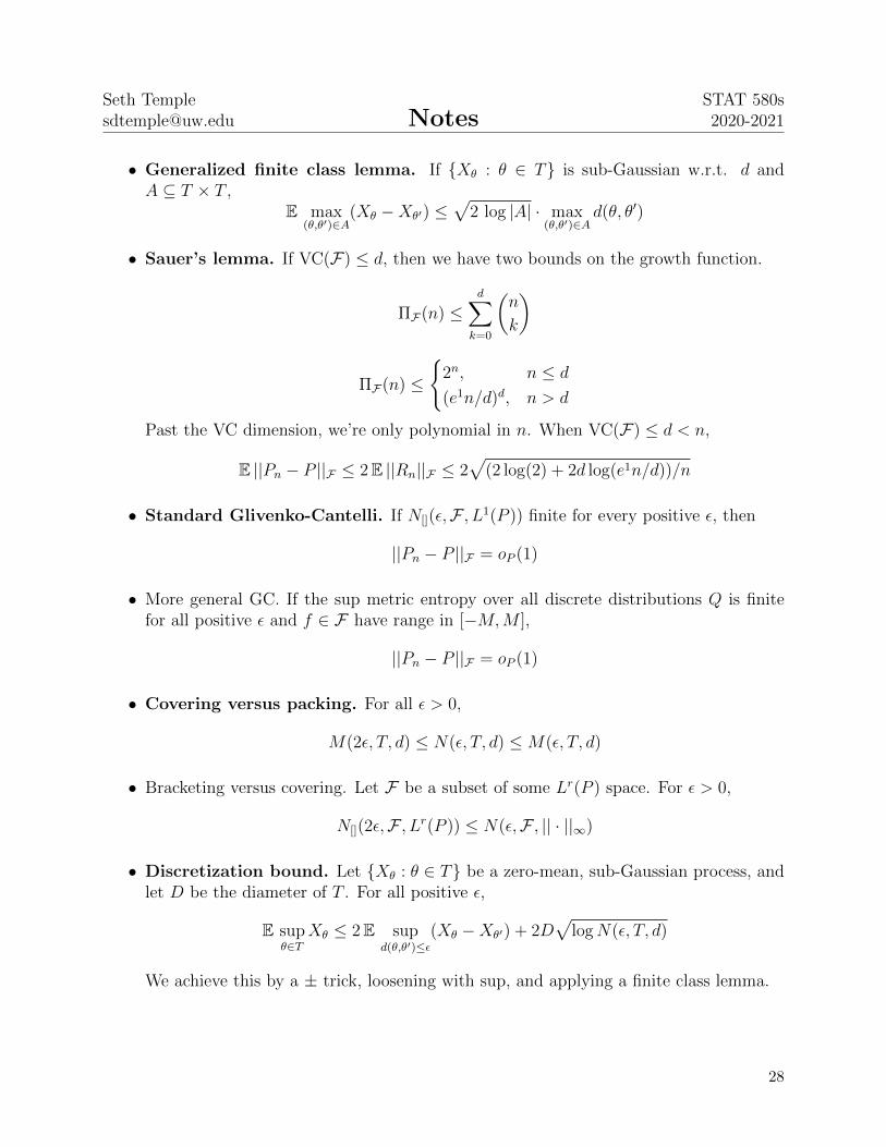
• Eight or more lemma. This lemma from Varshamov and Gilbert suggests thatsubsets of high-dimensional hypercubes exist such that the minimum Hamming distanceis large. Let Ω be an m-dimensional hypercube. If m ≥ 8, then |Ω| ≥ 2m/8 and theminimum Hamming distance is ≥ m/8. We take advantage of the implied inequalitiesin an example applying Fano’s method to a smooth regression problem.
• Pinsker’s inequality. For all distributions P1 and P2,
TV(P1, P2) ≤√
KL(P1, P2)/2
This belongs to a distribution distances heuristic involved in bound arguments.
• See slides 25-36 for applying Fano’s method to determine a tight lower bound for smoothregression problems. The K function on slide 27 is a bump function and m ≤ 1/h− 1such that bumps don’t overlap and the function is infinitely differentiable (very smooth).At various points the argument is to redefine constant terms ci and/or massage knowninequalities like those from the Varshamov-Gilbert lemma.
• In this example the minimum Hamming distance appears in formulas for the discrep-ancy and the KL divergence. The Hamming distance is the number of discordantpositions when comparing two byte strings.
• Applying Le Cam’s two-point method:
– For the mean θ of Rademacher random variables we derive r?n = n−1
– Density estimation from a Lipschitz class and normal errors we derive r?n = n−1/3
• Total variation TV is difficult to work with, so we often work with KL divergence viaPinsker’s inequality. When the KL divergence is large, an alternative bound providesa tighter lower bound for Le Cam’s method.
• The lower bound minimax rate for estimating Holder(β, L) density at a point is n−2β
2β+1 .
Figure 1: Distance metrics for probability distributions.
Kernel density estimators offer a upper bound for smooth density estimation that matchesthe lower bound rate, completing the argument for an optimal rate.
7.1 Definitions
• A kernel K : R → R satifies that∫K(u) du = 1. A kernel density estimator takes
form
fh(x) =1
nh
n∑i=1
K
(Xi − xh
)where bandwidth h is a tuning parameter. The bandwidth controls the smoothnessof the KDE, subsequently impacting the bias-variance tradeoff. Large h results in moresmoothing, larger bias, and smaller variance. Small h results in less smoothing, smallerbias, and larger variance.
• Up to s− 1, the moments of an sth-order kernel are zero and the sth moment is finite.
• Twicing is when we combine two related KDEs to get a KDE more amenable toconfidence intervals based on asymptotic normality.
4fh(x)− f2h(x)
3
7.2 Results
• The empirical cumulative distribution function is a good estimator for the CDF. How-ever, it is a step function, so its derivative is not an ideal estimator for the density.
• Kernel density estimators for Holder(β, L) smooth densities achieve upper bound rate
r?n n−2β
2β+1
Thus, the rate r?n is an optimal rate for Holder(β, L) density estimation. We arrive at
this upper bound by setting hn ∝ n−1
2β+1 , a compromise in managing bias squared and
variance. For d-dimensional densities, the rate is modified to n−2β
2β+d . An example ofthe “curve of dimensionality”.
• Kernel density derivative estimators have MSE bounded at rate n−2(β−1)2β+1
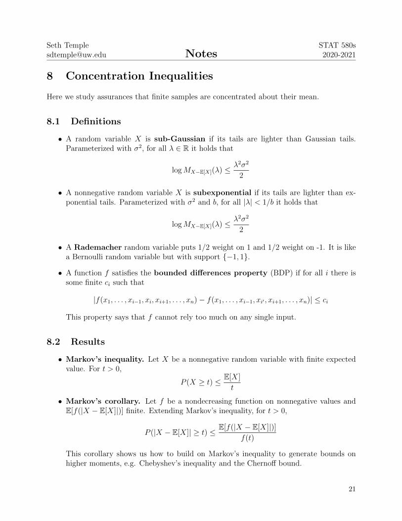
Here we study assurances that finite samples are concentrated about their mean.
8.1 Definitions
• A random variable X is sub-Gaussian if its tails are lighter than Gaussian tails.Parameterized with σ2, for all λ ∈ R it holds that
logMX−E[X](λ) ≤ λ2σ2
2
• A nonnegative random variable X is subexponential if its tails are lighter than ex-ponential tails. Parameterized with σ2 and b, for all |λ| < 1/b it holds that
logMX−E[X](λ) ≤ λ2σ2
2
• A Rademacher random variable puts 1/2 weight on 1 and 1/2 weight on -1. It is likea Bernoulli random variable but with support −1, 1.
• A function f satisfies the bounded differences property (BDP) if for all i there issome finite ci such that
• Chernoff bound. Suppose X has moment generating function in a neighborhood ofzero. For t > 0 and λ ∈ (0, b],
P (X − E[X] ≥ t) ≤ E[expλ(X − E[X])]eλt
=MX−E[X](λ)
eλt
P (X − E[X] ≥ t) ≤ infλ>0
MX−E[X](λ)
eλt
• Additivity of subexponentials and sub-Gaussians. This property is inheritedas a property of moment-generating functions when we have independent random vari-ables. See discussion on page 29 of Wainwright (2019). For independent subexponentialX1, . . . , Xn with parameters (σ2
i , bi), the sum of these is subexponential with parameters(∑n
i=1 σ2i ,maxi bi).
• Hoeffding’s inequality. This inequality applies to random variables with boundedsupport [a, b]. These random variables are sub-Gaussian with σ2 = (b − a)2/4. Thesecond statement uses independence to extend the result to a sample mean.
logP (X − E[X] ≥ t) ≤ − 2t2
(b− a)2
logP (Xn − E[Xn] ≥ t) ≤ − 2n2t2∑ni=1(bi − ai)2
• Tail bound for subexponentials. If X is subexponential with parameters (σ2, b),
logP (X − µ ≥ t) ≤
− t2
2σ2 , 0 ≤ t ≤ σ2/b
− t2b, t > σ2/b
This result suggests that the (right) tail probability in the exponent is quadratic in tfor small t and linear in t for large t. See an alternative presentation with proof asProposition 2.9 from Wainwright (2019).
• Bernstein’s inequality. LetX have finite variance σ2 and be bounded s.t. |X−µ| ≤ b.For all t > 0 we have
P (X ≥ µ+ t) ≤ exp
(− t2
2(σ2 + bt)
)If we have an independent collection of random variables so bounded and with possiblyunique mean and finite variances, then for all t > 0
P (Xn ≥ E[Xn] + t) ≤ exp
(− t2
2(bt+∑n
i=1 σ2i /n)
)Bernstein’s may be tighter than Hoeffding’s when variances are small.
• Bernstein’s expectation bound. Suppose we have a Bernstein-like tail inequality fornonnegative X. In Homework 3 Problem 1 we show
E[X] ≤ 2σ(√π +
√logC) + 4b(1 + logC)
where σ2, b > 0 and C ≥ 1.
• Bennet’s inequality. Given independent X1, . . . , Xn with zero mean, Xi ∈ [−b, b], andvariances σ2
i ,
P (X ≥ t) ≤ exp
(− nσ2
b2h
(bt
σ2
))where σ2 = 1/n
∑ni=1 σ
2i and h(y) = (1 + y) log(1 + y)− y for y ≥ 0. This inequality is
at least as tight as Bernstein’s. See Exercise 2.7 in Wainwright for a walkthrough.
• Efron-Stein inequality. Let f : X → R, and assume independent random variables.
Var(f(X)) ≤ 1
2
n∑i=1
E[(f(X)− f(X(i)))2]
=n∑i=1
E[(f(X)− E[f(X)|X(i)])2]
Further assumptions on f enable nicer forms on the bound. See homework 2. Provingthis involves a novel strategy.
• Bounded differences inequality. Let X = (X1, . . . , Xn) be an independent collec-tion of random variables and f satisfy BDP with bounds c1, . . . , cn. For t > 0 andE[|f(X)|] finite,
P (|f(X)− E[f(X)]| ≥ t) ≤ 2 exp
− 2t2∑n
i=1 c2i
This inequality is referred to as McDiarmid’s inequality. Proving it involves a noveltelescoping argument and the Azuma-Hoeffding inequality. See slides 34-39.
• Martingale differences inequality. Consider the martingale difference sequence:
• See Examples 2.11 and 2.12 in Wainwright (2019). Together these examples show howto reduce dimension based on a random projection while maintaining certain guaranteesabout the dimension reduction. This is done by leveraging properties of subexponentialχ2 random variables.
• See Slides 14-16 from Chapter 3 for a discussion of the Chernoff bound for normalrandom variables being in some sense aymptotically tight. Additionally, this exampleshows how to derive MGFs using a change of variables.
We establish tools to bound the regret in ERM by bounding empirical process terms, e.g.bounding the Rademacher complexity.
9.1 Definitions
• For a set Θ, an empirical risk minimizer θ is such that P`(θ) is close to infθ∈Θ P`(θ),denoting θ0 here as the arg min. In decision theory, we talk about θ as a parameter thatcharacterizes a parametric family. As a result, we look explicitly at the discrepancybetween θ and θ. Here we instead look at differences in expectation, introducing theterm regret:
Reg(θ) = P (`(θ))− P (`(θ0))
• A ghost sample is an independent (copy) sample X ′1, . . . , X′n used in Rademacher
symmetrization arguments. See Chapter 4 Part 1 Slides 13-18 for this technique.
• Let ε1, . . . , εn be Rademacher random variables, and define the Rademacher process
Rn :=1
n
n∑i=1
εif(Xi)
We denote ||Rn||F := supf∈F |Rn(f)| and call E ||Rn||F the Rademacher complexity.
• The growth function or shattering number measures the richness of the class F
ΠF(n) := supx1,...,xn
|Fx1,...,xn|
We discuss shattering in the context of function classes or sets. We say n points areshattered by F if ΠF(n) = 2n. Below are some properties of growth functions.
– ΠA(n+m) ≤ ΠA(n) ΠA(m)
– ΠA∪B(n) ≤ ΠA(n) + ΠB(n)
– ΠA∪B:A∈A,B∈B(n) ≤ ΠA(n) ΠB(n)
– ΠA∩B:A∈A,B∈B(n) ≤ ΠA(n) ΠB(n)
• The Vapnik-Chervonenkis (VC) dimension is the largest n such that a functionclass still shatters n points. The VC index is one plus the VC dimension, i.e. the firstn such that a function class can’t shatter n points. Write VC(F) as VC dimension ofF . We say a function class F (or set A) is VC if it has finite VC dimension. VC theoryis for classification problems.
• For r ≥ 1, Lr(P ) is the space of functions f s.t. ||f ||Lr(P ) := (∫|f(x)|r dP (x))1/r <∞.
The sup norm or uniform norm is supf∈F |f |.
• A Glivenko-Cantelli (GC) theorem is one where the implication is ||Pn−P ||F = oP (1).
• A bracket [`, u] is the set of f ∈ F s.t. ` ≤ f ≤ u pointwise. An ε-bracket is a bracket[`, u] satisfying ||u − `||Lr(P ) ≤ ε. The bracketing number N[](ε,F , Lr(P )) is theminimum cardinality of ε-brackets required to cover function class F .
• A pseudometric d, related to a metric, has ii) symmetry and iii) triangle inequality,but does not have i) the identity of indiscernibles. d(x, y) = 0 does not imply x = y.This is a more flexible quantity for discussing functions in Lr(P ) space.
• A subset T1 of a pseudometric space T is an ε-cover if for each θ ∈ T there is θ1 ∈ T1
s.t. d(θ1, θ) ≤ ε. Visually, T is a subset of a union of ε-balls centered at point inT1. The ε-covering number N(ε, T, d) is the minimum cardinality among possibleε-covers. The logarithm of the ε-covering number is refered to as the metric entropy.(We say T is totally bounded if for all positive ε there exists a finite ε-cover.)
• A subset T1 of a pseudometric space T is an ε-packing if d(θ, θ′) > ε for each pairθ, θ′ ∈ T1. Visually, ε-balls centered at points in T1 do not overlap. The ε-packingnumber M(ε, T, d) is the maximum cardinality among possible ε-packings.
• A stochastic process Xθ : θ ∈ T is a collection of (indexed) random variables. It iszero-mean if E[Xθ] = 0 for all indices θ. It is sub-Gaussian w.r.t. d if, for all pairsθ, θ′ ∈ T and for all λ ∈ R,
E[expλ(Xθ −Xθ′)] ≤ exp
(λ2d(θ, θ′)
2
)This generalizes sub-Gaussianity from Section 8 to stochastic processes.
• The canonical Rademacher process is a zero-mean, sub-Gaussian random process:
Xθ =n∑i=1
θiεi = 〈θ, ε〉
The canonical Gaussian process is a defined in the same fashion with ε1, . . . , εn beingstandard normals instead of Rademachers.
• The diameter D of a (pseudometric) space T is supθ,θ′ d(θ, θ′).
• An envelope function F for f ∈ F is s.t. |f | ≤ F pointwise.
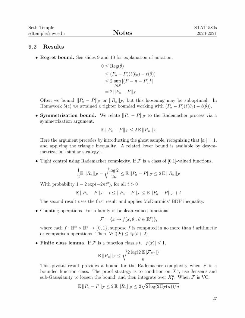
• Regret bound. See slides 9 and 10 for explanation of notation.
0 ≤ Reg(θ)
≤ (Pn − P )(`(θ0)− `(θ))≤ 2 sup
f∈F|(P − n− P )f |
= 2 ||Pn − P ||FOften we bound ||Pn − P ||F or ||Rn||F , but this loosening may be suboptimal. InHomework 5(c) we attained a tighter bounded working with (Pn − P )(`(θ0)− `(θ)).
• Symmetrization bound. We relate ||Pn − P ||F to the Rademacher process via asymmetrization argument.
E ||Pn − P ||F ≤ 2E ||Rn||F
Here the argument precedes by introducting the ghost sample, recognizing that |εi| = 1,and applying the triangle inequality. A related lower bound is available by desym-metrization (similar strategy).
• Tight control using Rademacher complexity. If F is a class of [0,1]-valued functions,
1
2E ||Rn||F −
√log 2
2n≤ E ||Pn − P ||F ≤ 2E ||Rn||F
With probability 1− 2 exp(−2nt2), for all t > 0
E ||Pn − P ||F − t ≤ ||Pn − P ||F ≤ E ||Pn − P ||F + t
The second result uses the first result and applies McDiarmids’ BDP inequality.
• Counting operations. For a family of boolean-valued functions
F = x 7→ f(x, θ : θ ∈ Rp),
where each f : Rm×Rp → 0, 1, suppose f is computed in no more than t arithmeticor comparison operations. Then, VC(F) ≤ 4p(t+ 2).
• Finite class lemma. If F is a function class s.t. |f(x)| ≤ 1,
E ||Rn||F ≤√
2 log(2E |FXn1|)
n
This pivotal result provides a bound for the Rademacher complexity when F is abounded function class. The proof strategy is to condition on Xn
1 , use Jensen’s andsub-Gaussianity to loosen the bound, and then integrate over Xn
• Chaining bound. Same setup as for the discretization bound. For all positive ε,
E supθ∈T
Xθ ≤ E supd(θ,θ′)≤ε
(Xθ −Xθ′) + 8
∫ D
ε/2
√log(N(δ, T, d)) dδ
For separable stochastic processes,
E supθ∈T
Xθ ≤ 8
∫ D
0
√logN(δ, T, d) dδ
Alex offered an extra lecture on proving the separable case. We achieve this by iter-atively applying a finite class lemma in a clever way. This bound is generally tighterthan the discretization bound.
• Chaining to control Rademacher complexity. If F is closed under negations,
E ||Rn||F ≤ 8n−1/2 E∫ ∞
0
√logN(δ,F , L2(Pn)) dδ ≤ 8n−1/2 sup
Q
∫ ∞0
√logN(δ,F , L2(Q)) dδ
• Bracketing integral bound. There is a universal positive constant C s.t for any class Fwith envelope function F ,
E ||Pn − P ||F ≤ Cn−1/2 ||F ||L2(P )
∫ 1
0
√logN[](δ||F ||L2(P ),F , L2(P )) dδ
9.3 Examples
• Vapnik-Chervonenkis (Some visuals)
– Dimension/index (Homework 3 Problem 4)
∗ (−∞, b] : b ∈ R has VC index 2.
∗ (−∞, b1]× (−∞, bd] : b1, . . . , bd ∈ R has VC index d+ 1
∗ (a1, b1]× (a1, , bd] : a1, . . . , ad, b1, . . . , bd ∈ R has VC index 2d+ 1
∗ (a, b] : a, b ∈ R has VC index 3.
∗ (a1, b1]× (a2, b2] : (a1, a2), (b1, b2) ∈ R2 has VC index 5.
∗ x 7→ g(x− θ) : θ ∈ R, g : R→ R monotone has VC index 2.
∗ Collection of convex sets in R2 has VC index ∞.
∗ x ∈ R2 : ||x− a||2 ≤ b has VC index 4.
– Applying the “counting operations” lemma
∗ Linear threshold class is VC
∗ Neural network classifiers are VC and we can attain probabilistic guaranteesfor regret (Homework 4 Problem 2)
We study the properties and applications of classes of random functions for which a uniformcentral limit theorem is available. (This section begins the transition from instructor AlexLuedtke to instructor Marco Sadinle.)
10.1 Definitions
• The empirical process Gn is√n(Pn − P ). When we apply it to functions f ∈ F , we
get a random variable. We study the stochastic process Gnf : f ∈ F.
• For measurable f and possibly nonmeasurable X, the outer expectation is
E∗[f(X)] = infE[U ] : U measurable, U ≥ f(X), and E[U ] exists
A similar definition works for inner expectation E∗. Outer and inner probabilities can bedefined using indicator functions. The measurability concerns related to these notionswe do not cover.
• A stochastic process Xn on F is called asymptotically uniform ρ-equicontinuousif, for all positive sequences δn → 0 and F(δn) = (f1, f2) : f1, f2 ∈ F , ρ(f1, f2) < δn,
supf1,f2∈F(δn)
|Xn(f1)−Xn(f2)| = oP (1)
Here the pseudometric ρ is important. With this sense of uniform continuity andconvergence in distribution of marginals, we achieve a weak convergence.
• A random variable X is tight if for every ε > 0 there is a compact set K such thatP (X ∈ K) ≥ 1− ε.
• An envelope function F is such that supf∈F |f(x)| ≤ F (x) for all x.
• If Gn G in `∞(F) where G is tight, then F is called P0-Donsker. This G is a mean-zero Gaussian process with covariance (f, g) 7→ EP0 [GfGg] = P0(fg)− P0(f)P0(g). Apseudometric guaranteed to exist is the standard deviation pseudometric:
ρ0 : (f1, f2) 7→√P0((f1 − f2)2)− (P0(f1 − f2))2.
• The variation norm of f : R → R is ||f ||V =∫|df(x)|. This measures all movement
along the y-axis. The uniform sectional variation norm ||f ||∗V of a function f : Rm → Rgeneralizes this univariate definition by considering generalized Riemann differences inslices. See slide 19 from chapter 0 notes, with special attention to the m = 2 case. Seevan der Laan’s 1996 thesis for more details.
• Generalized portmanteau. Let X1, X2, . . . be a sequence of arbitrary maps and Xbe another (random) map, all taking values in metric space (D, d). Weak convergenceXn X has many equivalent characterizations:
– E∗[f(Xn)]→ E[f(X)] for all bounded, continuous f .
– E∗[f(Xn)]→ E[f(X)] for all bounded, Lipschitz-continuous f .
– lim supn E∗[f(Xn)] ≤ E[f(Xn)] for every upper semicontinuous f bounded above.
– lim infnE∗[f(Xn)] ≥ E[f(X)] for every lower semicontinuous f bounded below.
– lim supn P∗(Xn ∈ F ) ≤ P (X ∈ F ) for all closed F .
– lim infn P∗(X ∈ O) for all open O.
– P ∗(Xn ∈ B)→ P (X ∈ B) for all continuity sets B.
This result is vdV Theorem 18.9 in the blue book. It is similar to our portmanteautheorem from our second section, but we use outer/inner expectations and probabilitiesfor possibly nonmeasurable maps.
• Generalized continuous mapping. Let (D, d) and (E, e) be metric spaces. Supposethat X1, X2, . . . are D-valued random variables, and that X is a D0-valued randomvariable with D0 ⊆ D. Let f : D → E be continuous on D0. Then, Xn X in Dimplies f(Xn) f(X) in E.
• Weak convergence equivalency. Xn converges weakly in `∞(F) to a tight randomvariable X if and only if
1. for each fj : j = 1, 2 . . . ,m ⊆ F we have Xn(fj) X(fj);2. there exists a pseudometric ρ on F such that
– (F , ρ) is totally bounded;
– Xn is asymptotically uniform ρ-equicontinuous.
The first condition is convergence in distribution of marginals. The second condition isthe existence of a suitable pseudometric such that F is not too rich and Xn is sufficientlysmooth. This result is from Theorems 1.5.4 and 1.5.7 of vdV&W (1996).
• A Slutsky result for . LetX1, . . . and Y1, . . . be sequences of `∞(F)-valued randomvariables for some function class F . If Xn X for some tight `∞(F)-valued X and||Xn − Yn||F = oP (1), then Yn X as well. (See Homework 0 Problem 1.)
• Controlling empirical process terms. To say that Gnfn = oP (1), it is sufficient toshow (1) P0f
2n = oP (1) and (2) fn is in a P0-Donsker class. (This is vdV lemma 19.24.
• Establishing Donsker classes. There are four strategies to establish a Donsker class.The brute force approach is work with the definition. The other three approachesinvolve entropy, permanence, and bounded variation. Entropy arguments via 582-typearguments are non-intuitive and challenging. Permanence arguments construct newDonsker classes from existing Donsker classes. Bounded variation arguments may bethe most useful.
– F is P0-Donsker if the bracketing integral J[](1,F , L2(P )) is finite.
J(δ,F , L2(P )) =
∫ δ
0
√logN[](ε,F , L2(P )) dε
– F is P0-Donsker if it has envelope F satisfying P0(F 2) <∞ and it has a uniformentropy bound. See slide 15 from Marco’s Chapter 0 and slide 57 from Alex’sChapter 4.2.
– Let F1, . . . ,Fk be P0-Donsker classes with ||P0||Fj < ∞ for j = 1, 2, . . . , k. Letφ : Rk → R for which there is C > 0 such that
|φ(f(x))− φ(g(x))|2 ≤ Ck∑j=1
|fj(x)− gj(x)|2
for every f, g ∈ F1, . . . ,Fk and x ∈ X . Then, φ (F1, . . . ,Fk) is P0-Donskerprovided φ (f1, . . . , fk) is P0-square integrable for some (f1, . . . , fk).
∗ If F and G are P0-Donsker classes and ||P0||F∪G finite, then pairwise infimaF ∧ G, pairwise suprema F ∨ G, and pairwise sums F + G are P0-Donskerclasses.
– For each positive constant M0, f : B ⊆ Rm → R : ||f ||∗V ≤ M0, P0(1B) = 1 is aP0-Donsker class.
∗ ||c · f ||∗V = c ||f ||∗V for any constant c > 0;
∗ ||f1 + f2||∗V ≤ ||f1||∗V + ||f2||∗V ;
∗ if f1 and f2 are bivariate cadlag functions, then |∫f1df2| ≤ 16 ||f1||∗V ||f2||∞;
∗ if f is bivariate, ||f ||∗V <∞, and f > δ > 0, then ||f−1||∗V <∞.
We establish language and results to talk about the asymptotic properties of estimators,especially to discuss joint behavior of two or more estimators.
11.1 Definitions
• Estimator ψn of ψ0 based on X1, . . . , Xn ∼ P0 ∈ M is said to be asymptoticallylinear if there is a function x 7→ φP0(x) such that
1. φP0(X) is mean-zero and has finite variance;
2. ψn−ψ0 = 1n
∑ni=1 φP0(Xi)+oP (n−1/2), where φP0 is the influence function. The
influence function expresses the extent to which outliers affect the estimator.
• The sandwich variance estimator in this context is
Σ :=1
n
n∑i=1
φP (Xi)φP (Xi)T ,
where P is a consistent estimator of P0.
• A V -statistic is an estimator for some generalized moment of a distribution; namely,
V (P ) :=
∫· · ·∫H(x1, . . . , xm) dP (x1) . . . dP (xm)
Vn := Pmn H
for some kernel function H. V -statistics may be biased in finite samples.
• A U -statistic is an unbiased estimator for some generalized moment of a distribution;
Un :=
(n
m
)−1 ∑im∈Dm,n
H(Xi1 , . . . , Xim)
Dm,n := im ⊆ 1, . . . , n : i1 < · · · < im
• Let P be a convex collection of distributions on R. Given F ∈ P , let Q(F ) be thevector space c(F1 − F ) : c ∈ R;F1 ∈ P equipped with some norm ρ. A functionΨ : P → R is ρ-continuous at F if, for any sequence F1, . . . ⊆ P , ρ(Fn − F ) → 0implies Ψ(Fn)→ Ψ(F ). This generalizes continuity for functionals.
• For any direction h ∈ Q(F ), the Gateaux derivative of Ψ at F ∈ F is
A functional Ψ is Gateaux differentiable at F ∈ F if Ψ(F ;h) exists for all h ∈ Q(F )and h 7→ Ψ(F ;h) is a linear functional.
• We study first-order representations like
Ψ(Fn)−Ψ(F0) = Ψ(F0;Fn − F0) + n−1/2Rn
Rn := RF0,εn(hn) = RF0,n−1/2(n1/2(Fn − F0))
RF,ε :=Ψ(F + εh)−Ψ(F )
ε− Ψ(F ;h)
If Rn = oP (1), we have asymptotic linearity. For this generalized asymptotic linearityof functionals, we require the above functional delta method.
• Suppose remainder term RF,ε tends to zero uniformly for h ∈ H and H ∈ H a collectionof subsets of Q(F ). That is, for each H ∈ H,
limε→0
[suph∈H|RF,ε(h)|
]= 0
We name different senses of uniform differentiability.
– Singleton (Gateaux) differentiability: H = singleton subsets of Q(F )– Compact (Hadamard) differentiability: H = compacts subsets of (Q(F ), ρ)– Bounded (Frechet) differentiability: H = bounded subsets of (Q(F ), ρ)
11.2 Results
• Delta method for influence curves. Let ψn be an asymptotically linear estimator ofψ0 ∈ Rp with influence curve φP0 . Suppose that h is differentiable at ψ0 with h′(ψ0) 6= 0.Then,
h(ψn)− h(ψ0) =1
n
n∑i=1
h′(ψ0)TφP0(Xi) + oP (n−1/2),
where x 7→ h′(ψ0)TφP0(x) is the new influence function.
• Delta method with a nuisance. Let X1, . . . , Xniid∼ P0. Consider some estimating
equation U(ψ, η)(x) such that (1) ψ0 is the unique solution P0U(ψ, η0) = 0, (2) ψnis a near-solution (PnU(ψn, ηn) = oP (n−1/2)), and (3) ηn is an asymptotically linearestimator of η0 with influence function ϕP0 . Then, provided some further regularityconditions, ψn is an asymptotically linear estimator of ψ0 with influence function
• Remainder Rn = oP (1) if either Ψ is compact differentiable at F0 relative to the supre-mum norm or Ψ is bounded differentiable w.r.t. some ρ and ρ(Fn − F0) = OP (n−1/2).
• (Pn − P0)f = Pnf − P0f = Pnf − PnP0f = Pn(f − P0f). This may be a term in aninfluence function after expanding terms with the ± trick.
We develop a general theory to study when asymptotically linear estimators achieve the lowestpossible asymptotic variance. This extends the observation of Charles Stein that estimationin a large modelM ought to be no easier than estimation in 1-dimensional parametric models.(Recall (Hajek’s) convolution theorem from Chapter 5 on optimal estimators.)
12.1 Definitions
• The (Fisher) information that parameter θ provides is
J (θ) := Pθ
([∂
∂θlog pθ
]2)This measures the curvature of the log-likelihood surface. Curvier surfaces have moredefinition to learn from.
• A generalized Cramer-Rao (GCR) lower bound depends on the information andpathwise derivatives with respect to sufficiently smooth models indexed by θ and passingthrough origin θ = 0.
σ20 ≥ sup
h∈H
[ ∂∂θ
Ψ(Pθ,h)|θ=0]2
JMh(0)
• Scores h ∈ H(P ) are defined (rigorously) with respect to quadratic mean differentiabil-ity (Chapter 3). Heuristically, if pθ,h = [1 + θh(x)]p(x) is sufficiently smooth, h is thederivative of the log density at θ = 0.
• The space L02(P ) is the collection of real-valued functions f with Pf = 0 and P (f 2) <∞
and endowed with the covariance inner product 〈f1, f2〉P . This is a Hilbert space.
• A (real) Hilbert space is a vector space equipped with an inner product and complete(in the Cauchy sense) relative to norm ||h|| := 〈h, h〉1/2. Some other properties are:
– Orthogonal complement H⊥0 of subspace H0 is h ∈ H : 〈h, h0〉 = 0,∀h0 ∈ H0– Projection of h ∈ H onto H∗, denoted Π[h|H∗], is the unique element h∗ ∈ H∗ s.t.
||h− h∗|| = min||h− h|| : h ∈ H∗
Residual h− h∗ is orthogonal to H∗, i.e. orthogonal to any h∗ ∈ H∗.– If H0 = H1 ⊕H2, then Π[·|H0] = Π[·|H1] + Π[·|H2]
– Given any closed subspace H0, H can be expressed as H0 ⊕ H⊥0 . As well, anyh ∈ H can be uniquely decomposed into h0 + h⊥0 .
– If Hf := cf : c ∈ R for some f ∈ H, then Π[h|Hf ] = 〈h,f〉〈f,f〉f for any h ∈ H.
– (Riesz representation) If φ is a bounded linear functional, there exists a uniqueelement h0 ∈ H s.t. φ(h) = 〈h, h0〉 for each h ∈ H. This representation offers theexistence of a gradient.
• The tangent set of model M at P is the set of (QMD) scores h ∈ L02(P ) for some
smooth 1-dim submodel indexed by θ that goes through the origin P at θ = 0.
• Tangent space, denoted TM(P ), is the additive and limit closure of the tangent set.Note that TM(P ) ⊆ L0
2(P ). Models are defined as nonparametric, semiparametric, andparametric according to the tangent space.
– Nonparametric: at each P the tangent space TM(P ) = L02(P )
– Parametric: if TM(P ) is finite-dimensional at each P ∈M– Semiparametric: otherwise
• A summary of interest Ψ :M→ R is pathwise differentiable at P ∈ M if there isa continuous linear map ΨP : L0
2(P )→ R s.t. for every h ∈ TM(P )
ΨP (h) :=∂
∂θΨ(Pθ,h)
∣∣∣∣θ=0
For each (regular) 1-dim parametric submodel Pθ,h : θ ∈ Θ through P the pathwisederivative at θ = 0 only depends on the score h.
• An element D(P ) ∈ L02(P ) is a gradient of Ψ at P relative toM if for each h ∈ TM(P )
ΨP (h) = 〈D(P ), h〉P
Given some gradient D0(P ), the set of gradients can be represented as
GM(P ) := D0(P ) + q(P ) : q(P ) ∈ TM(P )⊥)
The canonical gradient is the unique gradient D∗(P ) that lives in tangent spaceTM(P ). To find a gradient:
• Gradients in nested models. If M1 ⊆ M2, then GM2(P ) ⊆ GM1(P ). Pathwisederivatives are harder (there are less of them) when the model is larger.
• Influence functions are gradients. Suppose ψn is an asymptotically linear estimatorof ψ0 := Ψ(P0) with influence function φP0 . TFAE: (i) Ψ is pathwise differentiable atP0 and φP0 is a gradient, and (ii) ψn is regular at P0.
• Gradients are influence functions. Under sufficient regularity, for a gradient D(P0),TFAE: (i) an asymptotically linear estimator of ψ0 exists with influence function D(P0),and (ii) it is possible to estimate D(P0) consistently. This implies that we can find theinfluence function of an asymptotically linear estimator by computing a gradient.
• Canonical gradient is the efficient influence function. A RAL estimator ψn ofψ0 is efficient if and only if
ψn − ψ0 = Pn(D∗(P0)) + oP (n−1/2)
where D∗(P0) is the canonical gradient. This is established by looking at the GCRlower bound. We may refer to P0(D∗(P0)2) as the efficient bound.
12.3 Examples
• Simple 1-dim submodels
– pθ,h(x) := [1 + θh(x)]p(x)
– pθ,h(x) := exp(θh(x))p(x)/ch(θ) where ch(θ) is normalizing constant
– pθ,h(x) := expit(2θh(x))p(x)/ch(θ) where ch(θ) is normalizing constant
First approach usually suffices to compute a gradient. Third approach does not requirebounded h.
• Tangent spaces
– Nonparametric modelMµ for all d-variate distributions dominated by measure µ
– For bivariate M :=MZ ⊕MY |Z tangent space decomposes
TM(P ) = TMZ(P )⊕ TMY |Z (P )
For bivariate independence model, Y independent of Z,
TM(P ) = TMZ(P )⊕ TMY
(P )
See projections onto this tangent space in Note 5. Projections are verified bychecking orthogonality of residuals.
– Parametric M := Pβ : β ∈ B for some open, convex set B ⊆ Rp.
TM(P ) :=
x 7→ u · ∂
∂βlog pβ(x)
∣∣∣∣β=β0
: u ∈ Rp
See projections onto this tangent space in Note 5. Projections are verified bychecking orthogonality of residuals.
– A model with moment condition Pg0 = 0 for some g0
TM(P ) =
h ∈ L0
2(P ) :
∫g0(x)h(x)dP (x) = 0
See Homework 4 Problem 1 for more details on estimating ψ0 = Pf0 for some f0.This is an example in which the moment condition restricts the tangent space.
– A model for some symmetric distribution about some center/origin
TM(Pµ,f ) = T1(Pµ,f )⊕ T2(Pµ,f )
T1(Pµ,f ) := x 7→ af(x− µ)/f(x− µ) : a ∈ RT2(Pµ,f ) := x 7→ h(x− µ) : h ∈ H(P0,f )
See Homework 4 Problem 2 for more details on estimating the center µ0. This is ascenario in which exact knowledge about say f0 does not impact efficiency bound.
• Gradients
– Homework 4 Problem 1(c)
– Homework 4 Problem 2(b)
– General moment Ψ(P ) := Pf0 leads to D(P ) : x 7→ f0(x)− Pf0
– Average density value Ψ(P ) :=∫
[f(x)]2dx = Pf leads to D(P ) : x 7→ 2[f(x)−Pf ]after some calculus work
– Conditional mean value Ψ(P ) := E[Y |Z = z0]
D(P0) : (z, y) 7→ I(Z = z0)
P0(Z = z0)[y −Ψ(P0)]
See Note 6 for detail derivations. There is involved calculus work here.
• Differentiability in higher dimensions. Below are two representations of differen-tiability at ψ0. The first representation is especially useful for proving delta methods.For all ε > 0,
limε→0
sup||h||=1
|f(ψ0 + εh)− f(ψ)− ε〈h,∇f(ψ0)〉|ε
→ 0;
limh→0
||f(ψ0 + h)− f(ψ)− Jf (h)||||h||
→ 0.
Read more about the second representation at the Wikipedia article for differentiablefunctions in higher dimensions. A sufficient condition for differentiability is that partialderivatives exist and the linear map Jf is the Jacobian matrix. In class, we claimthis sufficient condition as that f is partially differentiable in a neighborhood aroundψ0 and the partial derivatives are continuous at ψ0. Lastly, note that h in the tworepresentations are different!
• Find a Lipschitz constant by finding the maximum of the norm of the gradient.
• Mean value theorem. For a function continuous on [a, b] and differentiable on (a, b)there is some c in the open interval such that the tangent line f ′(c) equals the secantline connecting a and b.
• Extreme value theorem. A continuous function on a closed interval attains itsmaximum and minimum values. With this result, we may assert that an extremum isat least attained.
• Fundamental theorems of calculus. These results link derivatives with integrals.
f(b)− f(a) =
∫ b
a
f ′(x) dx
f(x) =
∫ x
a
f(t) dt =⇒ f ′(x) = f(x)
• Taylor series. We approximate differentiable functions by the following and the re-mainder vanishes in the asymptote.
f(x) =f (0)(a)
0!(x− a)0 +
f (1)(a)
1!(x− a)1 +
f (2)(a)
2!(x− a)2 + remainder
• Lagrange remainder. Combining Taylor series with the mean value theorem wearrive at an alternative representation for `-differentiable functions.
f(x) =f (0)(a)
0!(x− a)0 +
f (1)(a)
1!(x− a)1 + · · ·+ f (`−1)(a)
(`− 1)!(x− a)`−1 +
f (`)(xa)
`!(xa)
`
Here xa is some point in the interval between x and a. Final term is Lagrange remainder.
• Bolzano-Weierstrass. Every bounded sequence has a convergent subsequence.
• Semi-continuity. See graphs under Examples.
– A function f is lower-semicontinuous at x0 if for all ε > 0 there is a neighborhoodaround x0 such that f(x) ≥ f(x0)− ε
– A function f is upper-semicontinuous at x0 if for all ε > 0 there is a neighborhoodaround x0 such that f(x) ≤ f(x0) + ε.
• Fisher-Cramer. This result from MDP’s STAT 513 says that the MLE is asymptot-ically consistant and normal if we have a regularity condition the depends of first andsecond derivatives of the log likelihood. Important estimators like medians may not fitinto this framework. We weaken this assumption using QMD.