sftfe: A Stata command for fixed-effects stochastic ... · f( y ij u )f( u ) d u (8) where is the...

Contribution to the communityConsistent estimation of the fixed-effects SF model

The sftfe commandMonte Carlo results

References

sftfe: A Stata command for fixed-effectsstochastic frontier models estimation

Federico Belotti? Giuseppe Ilardi

?CEIS, University of Rome Tor VergataBank of Italy

2014 Italian Stata Users Group MeetingMilan. November 13, 2014

Belotti, Ilardi Fixed-effects stochastic frontier estimation in Stata

Outline

1 Contribution to the community

2 Consistent estimation of the fixed-effects SF model

3 The sftfe command

4 Monte Carlo results



References

The fixed-effects stochastic frontier (SF) model

yit = αi + xitβ + εit , (1)

εit = vit − uit , i = 1, . . . , n, t = 1, . . . ,T , (2)

where, for each unit i and period t:

yit represents the output;

xit is a 1× k vector of exogenous inputs;

β is a k × 1 vector of technology parameters;

αi is the unit fixed-effect;

vit is the idiosyncratic error;

uit the one-sided disturbance which represents inefficiency.




References

Distributional assumptions - homoskedastic model

vit ∼ IID N (0, ψ2), (3)

uit ∼ IID Fu(µ, σ2), i = 1, . . . , n, t = 1, . . . ,T , (4)

vit and uit are independently distributed;

The inefficiency uit has distribution with support defined overR+, mean µ and variance parameter σ2 (e.g., half-normal(µ = 0), exponential (µ = σ) or truncated-normal);

vit is normally distributed with variance ψ2.




References

Heterogeneity

Heterogeneity: can be observable or unobservable;

Model (1)-(2) adds αi (unobservable) to shift the production(cost) function;

Observable heterogeneity is reflected in measured variables;

Examples are:1 Heteroskedastic inefficiency → σit = exp(zitδ);2 Heteroskedastic noise → ψit = exp(ritγ);3 Heterogeneity in the inefficiency mean → µit = sitξ;

It might be that zit = rit = sit .




References

The Maximum Dummy Variable approach

Greene (2005) propose to estimate model (1)−(4) by treatingthe unit-specific intercepts as parameters to be estimated;

This approach has been implemented in the sfpanel

command (Belotti et al., 2013);

However, as Greene’s simulations suggest, this approach leadsto inconsistent variance estimates, especially in short panels.

Since these parameters represent the key ingredients in thepost-estimation of inefficiencies, a solution to this issue iscrucial in the SF context.




References

Our contribution

The new command sftfe allows the estimation of the fixed-effectsSF models via three alternative estimators (Belotti and Ilardi, 2012;Chen et al., 2014)1;

They exploit the first-difference data transformation to eliminate thefixed-effects achieving consistency for both fixed-n and fixed-Tasymptotics;

sftfe allows to estimate models in which inefficiency follows afirst-order autoregressive process as well as to model inefficiency’svariance (eventually also the mean) as a function of exogenouscovariates.

1Belotti and Ilardi (2012) has been revised including the extension of the Chen et al. (2014) approach to

heteroskedastic and dynamic inefficiency models. The updated version is available fromhttp://www.econometrics.it.


http://www.econometrics.it



References

Eliminate the nuisance parameters

We get rid of the nuisance parameters through a first-differencedata transformation

∆yi = ∆Xiβ + ∆εi , (5)

∆εi = ∆vi −∆ui , (6)

where ∆yi = (∆yi2, . . . ,∆yiT ) with ∆yit = yit − yit−1 and ∆Xi isthe T − 1× k matrix of time-varying covariates with the t-th rowdenoted by ∆xit = (∆xit1, . . . ,∆xitk), ∀ t = 2, . . . ,T .




References

First-differenced modelIdiosyncratic error - ∆vi

The normality assumption for vit implies that ∆vi has aT − 1-variate normal distribution with covariance matrixΨ = ψ2ΛT−1, where ΛT−1 is

ΛT−1 =

2 −1 0 · · · 0−1 2 −1 · · · 0

0 −1. . .

. . ....

.... . .

. . .. . . −1

0 0 . . . −1 2

(7)




References

First-differenced model (ctd)Inefficiency - ∆ui

The multivariate distribution of ∆ui is generally unknown;

Nevertheless, given the independence assumption between∆vi and ∆ui , the marginal likelihood contribution L∗i can bedefined in general terms as

L∗i (θ) =

∫f (∆vi ,∆ui ) d∆ui =

∫f (∆vi )f (∆ui ) d∆ui

=

∫f (∆yi |∆ui )f (∆ui ) d∆ui (8)

where θ is the parameter vector to be estimated.




References

How to estimate the model: MMLE

Marginal Maximum Likelihood estimator (MMLE, Chenet al., 2014);

1 The basic idea is to exploit the Closed Skew Normal class ofdistributions (CSN, Gonzalez-Farias et al., 2004) that, thanks to itscloseness property under marginalization and linear transformations,allows to derive a closed form expression for the marginal likelihoodfunction in equation (8);

2 Feasible only when inefficiency has truncated-normal (orhalf-normal) distribution;

3 Extension to heteroskedastic (or dynamic) inefficiency iscumbersome when T > 5 since the estimation requires theapproximation of T-variate Gaussian integrals (see Kumbhakar andTsionas, 2011; Chen et al., 2014).




References

How to estimate the model: MMSLE

Marginal Maximum Simulated Likelihood estimator (MMSLE,Belotti and Ilardi, 2012);

1 The basic idea is that estimation can be accomplished viasimulation, treating the marginal likelihood function in equation (8)as an expectation with respect to the random vector ∆ui ;

2 Feasible when inefficiency has half-normal or exponentialdistribution;

3 Extension to heteroskedastic inefficiency is feasible but constrained(only time-invariant covariates can be used to model inefficiencyvariability);

4 Extension to dynamic inefficiency not feasible.




References

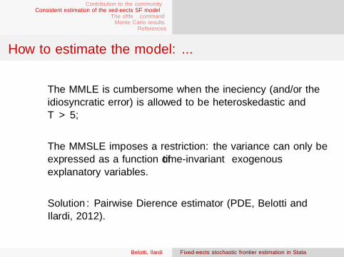
How to estimate the model: ...

The MMLE is cumbersome when the inefficiency (and/or theidiosyncratic error) is allowed to be heteroskedastic andT > 5;

The MMSLE imposes a restriction: the variance can only beexpressed as a function of time-invariant exogenousexplanatory variables.

Solution: Pairwise Difference estimator (PDE, Belotti andIlardi, 2012).




References

How to estimate the model: PDE

Pairwise Difference estimator (PDE, Belotti and Ilardi, 2012);

1 The basic idea is to exploit the closeness property of thenormal-exponential (or the normal-truncated normal via theCSN framework) marginal likelihood function when T = 2 todefine a U-estimator based on all pairwise quasi likelihoodcontributions;

2 Feasible and computationally efficient when inefficiency isheteroskedastic and has half-normal, exponential ortruncated-normal distribution;

3 Extension to dynamic inefficiency is feasible andstraightforward when the latter has truncated-normal (orhalf-normal) distribution.




References

The basic sftfe syntax is the following

sftfe depvar[indepvars

] [if] [

in] [

, options]

Factor variables are allowed.

Options:estimator(type) specifies the estimator to be used. May bemmle, mmsle and pde. Default is pde.

cost specifies a cost frontier model; default is production frontiermodel.




References

MMLE’s specific options

distribution(distname) specifies the inefficiencydistribution. Can be hnormal or tnormal. Default is hnormal.

ghkdraws([#] , [type(string) antithetics]) governs the drawsused in Geweke-Hajivassiliou-Keane (GHK) simulation ofhigher-dimensional cumulative multivariate normaldistributions. if # is omitted, the number of draws is set to100. The type(string) suboption specifies the type ofsequence in the simulation, can be halton, hammersley,ghalton, random, with halton being the default; antitheticsrequests antithetic draws; If this option is omitted, theestimation is performed exploiting the result outlined in Kotzet al. (2000) through Gauss-Hermite quadrature.




References

MMSLE’s specific options

distribution(distname) specifies the inefficiencydistribution. Can be exponential or hnormal. Default isexponential.

usigma(varlist [, noconstant]) specifies that inefficiency isheteroscedastic, with variance expressed as a function oftime-invariant covariates defined in varlist. Specifyingnoconstant suppresses the intercept in this function.




References

MMSLE’s specific options - 2

simtype(string) specifies the method to generate randomdraws for the first-differenced inefficiency. Can be uniform, foruniformly distributed random variates, or halton (the default)for Halton sequences.

nsimulations(#) specifies the number of draws used in thesimulation. The default is 250.

base(#) specifies the number, preferably a prime, used as abase for the generation of Halton sequences. The default is 5.




References

PDE’s specific options

distribution(distname) specifies the inefficiencydistribution. Can be exponential, hnormal or tnormal. Defaultis hnormal.

dynamic specifies that inefficiency follows a first-orderautoregressive process. Only when distribution(distname)is hnormal or tnormal.




References

PDE’s specific options - 2

emean(varlist m [, noconstant]) may be used only withdistribution(tnormal). With this option, sftfe specifiesthe inefficiency mean as a linear function of the covariatesdefined in varlist m.∗

usigma(varlist u [, noconstant]) specifies that inefficiency isheteroscedastic, with variance expressed as a function ofcovariates defined in varlist u.∗

vsigma(varlist v [, noconstant]) specifies that idiosyncraticerror is heteroscedastic, with variance expressed as a functionof covariates defined in varlist v.∗

∗ Specifying noconstant suppresses the constant in this function.




References

Postestimation

predict[type

]newvar

[if] [

in] [

, statistic]

where statistic includes:

xb, the default, calculates the linear prediction.

stdp calculates the standard error of the linear prediction.

u produces estimates of (technical or cost) inefficiency viaE(u|ε) using the Jondrow et al. (1982) estimator.

jlms produces estimates of (technical or cost) efficiency viaexp [−E(u|ε)].

alpha produces estimates of fixed-effects.




References

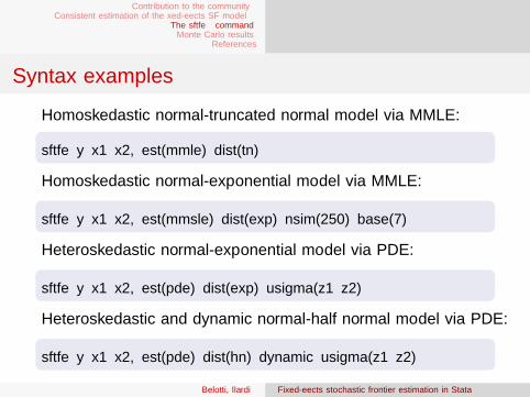
Syntax examples

Homoskedastic normal-truncated normal model via MMLE:

sftfe y x1 x2, est(mmle) dist(tn)

Homoskedastic normal-exponential model via MMLE:

sftfe y x1 x2, est(mmsle) dist(exp) nsim(250) base(7)

Heteroskedastic normal-exponential model via PDE:

sftfe y x1 x2, est(pde) dist(exp) usigma(z1 z2)

Heteroskedastic and dynamic normal-half normal model via PDE:

sftfe y x1 x2, est(pde) dist(hn) dynamic usigma(z1 z2)




References

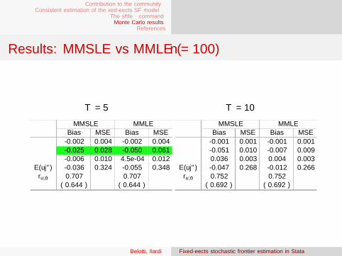
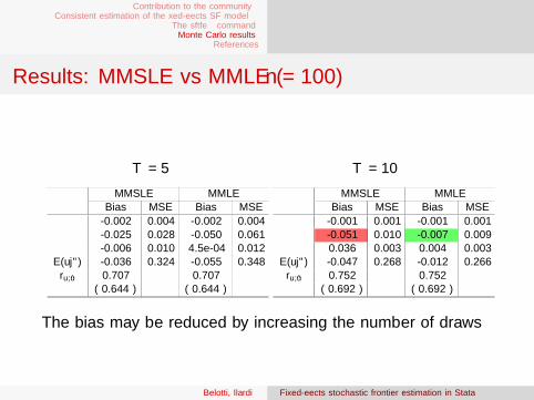
MMSLE vs MMLE - Data Generating Process

We consider the homoskedastic normal-half normal modelinvestigated by Chen et al. (2014), that is

yit = αi + βxit + vit − uit , (9)

vit ∼ N (0, ψ2), (10)

uit ∼ N+(0, σ2

)i = 1, . . . , n, t = 1, . . . ,T , (11)

wherethe fixed-effect parameters α1, ..., αn are drawn from a standard Gaussianrandom variable; xit = 0.5αi +

√0.52wit with wit ∼ N (0, 1);

For each experiment, we use the same αi and xit in all replications, thusonly uit and vit are redrawn in each replication;

We set β = 1, σψ

= λ = 2, and consider different sample sizes(n = 100, 250) and panel lengths (T = 5, 10);

The analysis is based on 250 replications for each experiment.




References

Results: MMSLE vs MMLE (n = 100)

T = 5

MMSLE MMLEBias MSE Bias MSE

β -0.002 0.004 -0.002 0.004σ -0.025 0.028 -0.050 0.061ψ -0.006 0.010 4.5e-04 0.012

E(u|ε) -0.036 0.324 -0.055 0.348ru,u 0.707 0.707

( 0.644 ) ( 0.644 )

T = 10


β -0.001 0.001 -0.001 0.001σ -0.051 0.010 -0.007 0.009ψ 0.036 0.003 0.004 0.003

E(u|ε) -0.047 0.268 -0.012 0.266ru,u 0.752 0.752

( 0.692 ) ( 0.692 )

The bias may be reduced by increasing the number of draws




References


T = 5


β -0.002 0.004 -0.002 0.004σ -0.025 0.028 -0.050 0.061ψ -0.006 0.010 4.5e-04 0.012

E(u|ε) -0.036 0.324 -0.055 0.348ru,u 0.707 0.707

( 0.644 ) ( 0.644 )

T = 10


β -0.001 0.001 -0.001 0.001σ -0.051 0.010 -0.007 0.009ψ 0.036 0.003 0.004 0.003

E(u|ε) -0.047 0.268 -0.012 0.266ru,u 0.752 0.752

( 0.692 ) ( 0.692 )





References


T = 5


β -0.002 0.004 -0.002 0.004σ -0.025 0.028 -0.050 0.061ψ -0.006 0.010 4.5e-04 0.012

E(u|ε) -0.036 0.324 -0.055 0.348ru,u 0.707 0.707

( 0.644 ) ( 0.644 )

T = 10


β -0.001 0.001 -0.001 0.001σ -0.051 0.010 -0.007 0.009ψ 0.036 0.003 0.004 0.003

E(u|ε) -0.047 0.268 -0.012 0.266ru,u 0.752 0.752

( 0.692 ) ( 0.692 )





References


T = 5


β -0.002 0.004 -0.002 0.004σ -0.025 0.028 -0.050 0.061ψ -0.006 0.010 4.5e-04 0.012

E(u|ε) -0.036 0.324 -0.055 0.348ru,u 0.707 0.707

( 0.644 ) ( 0.644 )

T = 10


β -0.001 0.001 -0.001 0.001σ -0.051 0.010 -0.007 0.009ψ 0.036 0.003 0.004 0.003

E(u|ε) -0.047 0.268 -0.012 0.266ru,u 0.752 0.752

( 0.692 ) ( 0.692 )





References


T = 5


β -0.002 0.004 -0.002 0.004σ -0.025 0.028 -0.050 0.061ψ -0.006 0.010 4.5e-04 0.012

E(u|ε) -0.036 0.324 -0.055 0.348ru,u 0.707 0.707

( 0.644 ) ( 0.644 )

T = 10


β -0.001 0.001 -0.001 0.001σ -0.051 0.010 -0.007 0.009ψ 0.036 0.003 0.004 0.003

E(u|ε) -0.047 0.268 -0.012 0.266ru,u 0.752 0.752

( 0.692 ) ( 0.692 )





References


T = 5


β -0.002 0.004 -0.002 0.004σ -0.025 0.028 -0.050 0.061ψ -0.006 0.010 4.5e-04 0.012

E(u|ε) -0.036 0.324 -0.055 0.348ru,u 0.707 0.707

( 0.644 ) ( 0.644 )

T = 10


β -0.001 0.001 -0.001 0.001σ -0.051 0.010 -0.007 0.009ψ 0.036 0.003 0.004 0.003

E(u|ε) -0.047 0.268 -0.012 0.266ru,u 0.752 0.752

( 0.692 ) ( 0.692 )





References


T = 5


β 0.001 0.001 0.001 0.001σ 0.002 0.011 0.001 0.012ψ -0.011 0.004 -0.011 0.005

E(u|ε) -0.016 0.304 -0.017 0.305ru,u 0.711 0.711

( 0.651 ) ( 0.651 )

T = 10


β 0.001 3.7e-04 8.8e-04 3.6e-04σ -0.025 0.004 -0.004 0.004ψ 0.016 0.001 -2.9e-04 0.001

E(u|ε) -0.026 0.261 -0.009 0.261ru,u 0.752 0.752

( 0.691 ) ( 0.691 )




References

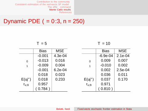
Dynamic PDE - Data Generating Process

We specify the following heteroskedastic normal-half normal modelwith AR(1) inefficiencies

yi = αi ιT + βxi + vi − ui , (12)

vi ∼ NT (0, ψ2It), (13)

ui ∼ N+T

(0, (1− ρ2)−1Ωi

), i = 1, . . . , n, (14)

whereΩi = ωitst,s=1,...,T with ωits = σitσisρ

|t−s| and σit = exp(γ0 + zitγ1);

α1, ..., αn and zit are drawn from a standard Gaussian random variablewhile xit = 0.5αi +

√0.52wit with wit ∼ N (0, 1);

We set β = 0.5, ψ = 0.5, γ0 = −0.5 and γ1 = 1 (this impliesλ = 1

nTψ

∑ni=1

∑Tt=1 σit ≈ 2).




References

Dynamic PDE - Data Generating Process

The simulation of the inefficiency vector ui is performed usingthe MCMC approach outlined in Geweke (1991), which uses aGibbs algorithm for sampling from an arbitrary multivariatetruncated normal distribution;

We consider two different values for the ρ parameter(ρ = 0.3, 0.7), different sample sizes (n = 100, 250) and panellengths (T = 5, 10);

The analysis is based on 250 replications for each experiment.




References

Dynamic PDE (ρ = 0.3, n = 100)

T = 5

Bias MSE

β -0.002 0.001γ0 -0.061 0.051γ1 -0.013 0.011ψ -0.002 0.001ρ 0.071 0.039

E(u|ε) 0.028 0.249ru,u 0.952

( 0.781 )

T = 10

Bias MSE

β -7.8e-04 5.5e-04γ0 -0.009 0.019γ1 -0.004 0.005ψ 5.4e-04 6.0e-04ρ 0.034 0.024

E(u|ε) 0.032 0.173ru,u 0.970

( 0.806 )




References


T = 5

Bias MSE

β -0.001 4.3e-04γ0 -0.013 0.016γ1 -0.009 0.004ψ -0.001 6.2e-04ρ 0.018 0.023

E(u|ε) 0.018 0.233ru,u 0.957

( 0.784 )

T = 10

Bias MSE

β -6.9e-04 2.1e-04γ0 0.009 0.007γ1 -0.010 0.002ψ 0.002 2.5e-04ρ 0.036 0.011

E(u|ε) 0.037 0.170ru,u 0.971

( 0.810 )




References


T = 5

Bias MSE

β -0.003 0.001γ0 -0.220 0.104γ1 -0.012 0.007ψ -6.3e-04 0.002ρ -0.008 0.010

E(u|ε) -0.123 0.515ru,u 0.955

( 0.800 )

T = 10

Bias MSE

β -9.7e-04 7.2e-04γ0 -0.088 0.030γ1 -0.010 0.003ψ 0.002 7.1e-04ρ -0.019 0.004

E(u|ε) -0.050 0.346ru,u 0.974

( 0.838 )




References


T = 5

Bias MSE

β -0.001 5.2e-04γ0 -0.180 0.054γ1 -0.012 0.003ψ -0.002 7.1e-04ρ -0.011 0.004

E(u|ε) -0.106 0.496ru,u 0.959

( 0.801 )

T = 10

Bias MSE

β -3.9e-04 2.5e-04γ0 -0.073 0.012γ1 -0.013 0.001ψ 0.002 3.0e-04ρ -0.019 0.002

E(u|ε) -0.039 0.336ru,u 0.975

( 0.842 )




References

References

Belotti, F., Daidone, S., Ilardi, G., and Atella, V. (2013). Stochastic frontier analysis using Stata. Stata Journal,13(4):718–758.

Belotti, F. and Ilardi, G. (2012). CEIS Research Paper 231, Tor Vergata University, CEIS.

Chen, Y., Wang, H., and Schmidt, P. (2014). Consistent estimation of the fixed effects stochastic frontier model.Journal of Econometrics, 181(2):65–76.

Geweke, J. (1991). Efficient simulation from the multivariate normal and student-t distributions subject to linearconstraints and the evaluation of constraint probabilities. In Keramidas, E. M., editor, Computing Science andStatistics: Proceedings of the 23rd Symposium on the Interface, pages 571–578. Interface Foundation of NorthAmerica, Inc.

Gonzalez-Farias, G., Dominguez-Molina, J., and Gupta, A. (2004). Additive properties of skew normal randomvectors. Journal of Statistical Planning and Inference, 126:521–534.

Greene, W. (2005). Reconsidering heterogeneity in panel data estimators of the stochastic frontier model. Journalof Econometrics, 126:269–303.

Jondrow, J., Lovell, C., Materov, I., and Schmidt, P. (1982). On the estimation of technical efficiency in thestochastic production function model. Journal of Econometrics, 19:233–238.

Kotz, S., Balakrishnan, N., and Johnson, N. L. (2000). Continuous Multivariate Distributions, Volume 1, Models

and Applications, 2nd Edition. John Wiley & Sons.

Kumbhakar, S. C. and Tsionas, E. G. (2011). Some recent developments in efficiency measurement in stochasticfrontier models. Journal of Probability and Statistics, 2011.


Date post:	29-Jan-2020
Category:	Documents
Upload:	others
View:	6 times
Download:	0 times

sftfe: A Stata command for fixed-effects stochastic ... · f( y ij u )f( u ) d u (8) where is the...

Documents