1

Shadow wages for the EU regions

Chiara Del Bo, Carlo Fiorio, Massimo Florio1 DEAS, Università degli Studi di Milano2

Abstract

According to cost-benefit analysis theory, the shadow wage rate (SWR) is the social opportunity cost of labour. After

reviewing earlier theoretical and empirical literature, we define the SWR under four labour market conditions: fairly socially

efficient (FSE), quasi-Keynesian unemployment (QKU), urban labour dualism (ULD) and rural labour dualism (RLD). We

offer, for the first time to date, a shortcut empirical estimation of the shadow wages for the EU at the regional (NUTS2) level.

Our estimated values are in the form of conversion factors, i.e coefficients that translate actual observed real wages into

shadow wages, as required by the evaluation of public investment projects under the Structural Funds of the EU. Our results

are obtained with an empirical strategy that is easy to implement with aggregate regional data, differently from traditional

micro-data based approaches to the estimation of the SWR, that are costly, project specific, and often difficult to be applied

because of lack of information.

We find that the conversion factor for the shadow wage rate is approximately 0.99 in 63 FSE regions (mostly in regions with

capital cities and in the old EU member states, where unemployment is low); 0.80 in 129 ULD regions, where there are both

migration inflows and unemployment ; 0.54 in 52 QKU regions, where unemployment is high; and 0.62 in 22 RLD regions

(mainly in Eastern European countries, where the share of rural employment and migration outflows are high). These

findings point to a high variability of labour market regimes in the EU and have important implications for project evaluation.

JEL Codes: H43, D61, R23

Keywords: Shadow wage, project evaluation, EU regions

1. Introduction

The shadow wage rate is the social opportunity cost of labour, and may differ from the observed

wage because of distortions in the labour market and in product markets as well. Under the wide scope

of EU regional policy and support to public investment in the New Member States there is now a

renewed interest in the estimation of shadow wages (European Commission (2008), Florio (2006)).

In the practice of cost-benefit analysis, observed market wages are translated into shadow wages

by conversion factors. These are coefficients computed as the ratio between the shadow and market

1 chiara.delbo@unimi.it (corresponding author), carlo.fiorio@unimi.it, massimo.florio@unimi.it 2 An earlier version of this paper was presented at the VII Milan European Economy Workshop, June 11th and 12th, 2009, University of Milan, in the framework of the EIBURS project, sponsored by the European Investment Bank. The Authors gratefully acknowledge the EIBURS financial support. The usual disclaimer applies and the views of the Authors do not necessarily reflect those of the EIB. The authors are grateful for comments on an earlier draft to Gines De Rus, Gareth Myles and Silvia Salini, and wish to thank Julien Bollati for competent research assistance. The usual disclaimer applies.

2

wage. In this paper we provide, for the first time to date, an estimation of conversion factors for the

calculation of shadow wages a regional level for the 27 member state of the EU. Moreover, we aim at

reviving the interest on a crucial ingredient of cost-benefit analysis. The definition and calculation of the

shadow wage rate was an important research topic in applied welfare economics since the 1960s (see,

inter alia, Little (1961), Sen (1966, 1972), Harberger (1971), Lal (1973), Little and Mirrlees (1974), Sah

and Stiglitz (1985). More recently shadow wages have been discussed inter alia by Potts (2002),

Londero (2003) and de Rus (2010), who propose shortcut approaches. Actual estimation and practical

applications of shadow pricing in general, and particularly of the SWR, in fact, have been limited, as

critically discussed, for example, by Squire (1998) or Little and Mirrlees (1990), in spite of the

requirements of project evaluation by international organizations, e.g. World Bank (2010), European

Commission (2008), Asian Development Bank (1997), or national governments, e.g. Honohan (1998)

for Ireland, De Borger (1993) for Belgium, Treasury Board of Canada (2002), or Saleh (2004) for

Australia. One reason for the difficulty of translating shadow wage theory into practice is the heavy

information burden for evaluators, who are often required to use project-specific micro-data, such as

surveys of reservation wages or firm-level marginal productivity.

In this paper we aim at deriving a new simple framework for the empirical computation of

shadow wages and conversion factors at the regional level, accounting for structural characteristics and

labour market conditions. We argue that shadow wages differ in space due to underlying spatial

economic, demographic and labour market structures. To do so, we propose to estimate a set of shortcut

shadow wage formulae based on solid theoretical grounds, that are, at the same time, easily

implementable with regional and national statistical data, moving away from the more precise but

cumbersome and costly approaches based on project-specific micro-data. We believe that the benefit of

relying on official statistics is worth the cost of a less precise computation of the shadow wage rate. We

regard this as a first step in order to provide project evaluators, particularly in the NMS of the EU and in

the context of regional policy, with a range of indicative values. Then, where needed and if possible,

evaluators may go ahead with the more information-demanding empirical approaches, usually based on

survey data and other local evidence.

Our approach is explicitly based on well established CBA theory, particularly on a combination

of the Little and Mirlees (1974) and the Drèze and Stern (1987,1990) frameworks.

After a brief review of the theoretical and empirical literature, we define four regional labour

market conditions in the EU, that differ in terms of per capita GDP, short and long term unemployment,

migration, and the role of agriculture in the regional economy. Our taxonomy along these five main

dimensions can be summarized as follows: fairly socially efficient (FSE), where labour is paid its

marginal product and unemployment is frictional; quasi-Keynesian unemployment (QKU) with wage

3

rigidities and high officially recorded unemployment rate; urban labour dualism (ULD) where the urban

informal labour market attracts workers from the rural areas, in spite of relatively high unemployment;

and rural labour dualism (RLD) where excess labour supply is partly absorbed by the agriculture sector,

and there is high migration to other regions. We then identify EU regions belonging to the four different

labour market conditions by means of a robust cluster analysis and compute shadow wages and the

corresponding conversion factors for each region in 2007.

As the conversion factor is defined as the ratio between the shadow wage and the observed

market wage, if the shadow wage is, for example, of 10,000 Euro and the conversion factor is equal to

0.85, the market wage is greater than the shadow wage, which is only Euro 8,500, hence the social

profitability of the public project is greater when labour is correctly evaluated at its social opportunity

cost. For many infrastructure projects, ignoring this correction may lead to an underestimation of the

social benefits of public investment.

Moreover, our findings highlight a substantial degree of SWR variability between European

regions, with important implications for public project evaluation and for the allocation of the EU

Structural Funds. In fact, we find that the numerical estimate for the conversion factor is of 0.99 in 63

FSE regions (mostly in regions with capital cities and in the old EU member states); 0.80 in 129 ULD

regions; 0.54 in 52 QKU regions, and 0.62 in 22 RLD regions (mainly in Eastern European countries).

The dispersion around these averages is, however, rather high for some subsets and this justifies the

computation of region-specific conversion factors.

The next Section presents an overview of earlier literature on shadow wages, both from a

theoretical and empirical perspective and provides a critical discussion of the state of the art in the field.

Section 3 lies out the conceptual framework for our analysis. Sections 4 and 5 present the data used, the

empirical analysis, and results. Finally, Section 6 summarizes and concludes. We derive some of the

formulae in an Appendix.

2. Earlier literature and research motivation

A project that uses labour as an input must normally consider this fact as a social cost, in the

same way as financial analysis considers the wage paid as a financial outflow. In principle, the social

opportunity cost of additional project employment is either the value, given a numeraire, of the marginal

product of labour in the economy, or the worker’s subjective disutility of effort. In principle, the two

measures would coincide for an equilibrium labour market, and would be equal to the observable market

wage. Nevertheless, even under full employment and in a competitive labour market, the market wage

may differ from the shadow wage because of the social cost of displacing workers from an activity to

4

another and because of price distortions in other markets. Moreover, labour markets are often far from

being in equilibrium, and close with unemployment and/or migration.

The CBA literature offers different shadow wage formulae based on different hypotheses on

labour market conditions, and sometimes on capital and product markets as well. This makes

comparisons across results often difficult. In this Section we provide a concise picture of early

contributions and recent findings on the social cost of labour.

In one of the earliest contributions, Lewis (1954) proposed a simple closed economy model based on

output loss. Society maximizes aggregate output, and consumption of different workers is given equal

social weight by the government. Employment per se has no social value (for a different view on this

issue, see Brent (1991)), the unemployed do not receive any subsidy, and leisure is given no value,

implying the lack of a term capturing the disutility of effort. The main message is that the shadow wage

is equal to the lost output from the former employment, i.e. the value of the marginal product of the

sector of provenance (that will be the one with the lowest wages at the end of the vacancy-replacement

chain, e.g. agriculture). With high unemployment or marginal productivity in the previous occupation

equal to zero, the new job created has no real effect in other sectors of the economy. The project

displaces some workers and hires some unemployed, in a proportion that represents the share of

employed and unemployed in the economy. These ideas are now frequently encountered in later applied

papers, e.g. see Campbell and Tobal (1981) in the context of projects by international organizations in

developing nations and by the Water Resources Council in the US. We shall see later the empirical

implications of this early shadow wage concept.

Going back to shadow wage theory, a classical starting point in the context of project evaluation

was the important work by Little and Mirrlees (1974), henceforth LM, drawing from their previous

OECD guidelines for project appraisal in developing economies. The authors justify the use of shadow

prices because of the presence of real wage rigidity in the formal sector of the economy, which

exaggerates the social cost of employment. Specifically, they identify five main sources of distortion.

First, even if actual wages were equal to the value of the marginal product of labour at market prices, the

former may be distorted by taxes and subsidies: hence consumption at shadow prices may be greater or

less than that at market prices. Second, labour in the rural sector receives subsidies (one may think of the

Common Agricultural Policy of the EU as a significant example). Third, in the formal sector there are

minimum wage requirements because of government regulation or unionization that may distort the

market. Finally, in some sectors high wages may correspond to even higher productivity and

consumption and transferring labour from the rural sector to the urban or formal sector may entail some

costs. This situation can be described as a combination of classical unemployment and dualism. We will

5

present and discuss the LM framework in more detail in Section 3, as their formulae will be the starting

point for our models.

Other theoretical contributions include in the vein of general equilibrium public economics

Marchand et al. (1984), who study the interrelations between the shadow wage rate and the social

discount rate. They consider an economy with one consumer, two consumption goods offered by a

competitive public sector, leisure, and a benevolent government. There is wage rigidity and involuntary

unemployment, while the interest rate is flexible. Expanding public expenditures financed by lump-sum

taxes gradually closes the gap between shadow and market wages. However, if there is displacement of

private investment and employment, the social discount rate may be greater than the interest rate.

Moreover, with distortionary taxation, e.g. profit taxation, there is both rationing in the labor market, and

a wedge between the gross and net of tax cost of capital. This work is an example of the complex

interrelation between the SWR and other ingredients of cost-benefit analysis, even in a very simple

economic model. This shows the limitation of the typical partial equilibrium approaches, such as those

presented in several textbook version of CBA (e.g. Boardman et al., 2003).

The problem with general equilibrium shadow wage rates is that the models tend to be very

complex, and the results sometimes surprising. An example is Roberts (1982), who shows that in an

economy with labor rationing, wage rigidity, flexible prices for goods, savings and money balances, one

public good, lump sum, profit and indirect taxation, the shadow wage can even be negative under very

high unemployment. This model is one of the few on the CBA literature where government may have a

monetary policy, and public production can be financed either by money, indirect or lump taxes. In this

context, under money finance, a high reservation wage, and high marginal propensity to consume, the

sign of the shadow wage is reversed: a public good production at shadow prices is the more desirable the

more it is unprofitable at producer prices. Another example of complex results is provided by Johansson

(1982), who proposes a model of a small open economy with three private firms, producing three goods

(one exported, one imported, one non traded), one public firm offering a non traded good, labour and

money. This setting potentially generates 24 rationing equilibria (for each good there may be either

excess demand or supply, given the n-1 conditions constraining the remaining market). Johansson offers

welfare measures, hence shadow prices, for four cases based on Malinvaud, (1977): Walrasian

equilibrium, ‘orthodox’ Keynesian unemployment (wage rigidity, price flexibility), fix-price Keynesian

unemployment (widespread price rigidity, except the exchange rate, excess supply in both product and

labour markets) and classical unemployment (excess labour supply combined with excess demand of

goods). Welfare measures are shown to be different in the four cases. Burgess (1989) considers the

relationship between the social opportunity cost of capital in the private sector and the gross-of-tax

return to capital when tax-induced labour market distortions cause the prevailing market wage to exceed

6

the social opportunity cost of labour (shadow wage).The main finding is that only part of the excess of

the market wage over the social opportunity cost of labour should be attributed to the private sector if

public investment can be considered as an input in private sector’s production processes, thus implying

that the social opportunity cost of capital is a function of the marginal product of capital in the private

sector and of the wedge between the market and shadow wage.

The CBA general equilibrium framework is admirably summarized by Drèze and Stern, (1987,

and 1990). Drèze and Stern (henceforth, DS) explicitly define shadow prices, including the SWR, as the

solution of a planning problem in second best economies. Their discussion generalises much of the

earlier debate, and in spite of the complexity of their results, still offers potentially testable ideas. We

shall consider each of the DS shadow wage formulas in Section 3 and in the Appendix, and use them as

the basis for our empirical application.

Another strand of SWR literature stemmed from the work by Harris and Todaro (1970), and

Harberger (1971), which consider the role of trade and migration. The basic Harris and Todaro,

henceforth HT, framework is described by a two sector static model, with internal trade and

unemployment. The main idea is that workers of the rural sector with lower productivity (i.e. income)

migrate to the urban sector, despite unemployment, until the urban expected wage equals the rural

certain wage. In this context, the proportion of employed on the total labour force represents the

probability of being hired. The main conclusion therefore is that the shadow wage will equal the market

wage if the unemployment rate remains unchanged. Fitzgerald (1976) introduces a petty urban service

sector, and defines a more complex saving cost concept. We shall adopt the idea of an urban informal

sector in one of our empirical formulas. An early analysis of a two sector model, with a traditional

agriculture sector and the government project sector, is given by Warr (1973). Mazumdar (1976)

proposes a different migration equation that allows for different methods of financing the period of

urban job research (e.g. income support by rural family or self financing with informal activities in the

urban sector). The dynamic equilibrium obtained is shown to be a particular form of the LM solution.

The result, with stringent conditions, could theoretically give a shadow wage greater than the market

wage. On this issue, see also Gupta (1986).

This setting has been further extended in the Sah and Stiglitz (1985) contribution, which presents

a general equilibrium model for shadow wages in developing countries. Shadow wages are influenced by

the structure of industrial and agricultural sectors, by the nature of the international trade environment

and by the equilibrating mechanism of the model. The derived relationship between shadow wages and

market wages can be adapted to various technological and institutional frameworks which are country-

specific. Another interesting extension to the HT model was proposed by economists aiming at a

conceptually relevant formula for efficient regional employment policies in Canada. Boadway and

7

Flatters (1981), and later on Wilson (1993), describe poor regions as those with fixed wages and

unemployment while rich regions are characterized by full employment and self-adjusting productivity.

The shadow wage in these models includes output loss along with changes in the imputed value of

leisure and migration costs from taking workers from the labour market.

What appears from these studies is that unemployment per se may not be sufficient to guarantee a

shadow wage lower than the market wage because of migration phenomena.

It is apparent from this brief and very selective review of early theoretical literature that it is not

possible to compute shadow wages, and thus infer the social cost of labour, without a model of the

underlying labour market, including at least a simple theory of wage determination and migration. In

principle, there are subtle interrelations of the SWR with the capital and product markets as well, an

issue that we do not deal with in this paper, except that for the inclusion in our analysis of a correction

for price distortions in agriculture products.

We now turn briefly to the empirical literature. When the shadow wage is simply seen as the

marginal productivity of labour, as in earlier theories, it can be directly estimated using a production

function. Cobb-Douglas specifications are often used in models estimating the labour supply of members

of agricultural households, especially in developing economies. A very good example of this approach is

Jacoby (1993) who uses data on 1034 households in 1985-86 from the Peruvian highlands region and

finds that testing the equality between wages and marginal product, leads to estimates of the conversion

factor between 0.37 and 0.58. Skoufias (1994) considers data from six villages in India from rainy

season crop-cycle of the calendar years 1975-1979. This leads to a total of 675 farmer/year estimation in

166 households and a conversion factor of 0.83 for males and 0.63 for female workers. Adbulai and

Regmi’s (2000) analysis is based on a cross-sectional survey of 280 farm households in Nepal from May

1996 to April 1997. Eight villages were selected representing the three agro climatic zones of the

country and they estimate a conversion factor of 0.414. See also Lal (1979) who estimates shadow prices

for Jamaica, and finds a conversion factor of 0.73. In a study on child labour, Menon et al. (2005)

estimate the shadow wage using a cost function that treats household labour as a quasi-fixed factor,

using data from the Nepal Living Standard Survey (1996) along with additional estimations carried out

on a sample of 2,380 farm households. Their main results are that, considering families with working

children, the adults’ shadow wage is below the market wage, implying a conversion factor well below

unity. A very comprehensive computation of shadow prices for Colombia is offered by Londero (2003),

who considers skilled and unskilled labour, foreign labour, administrative and professional jobs, and

8

differences in the level of benefits, with conversion factors ranging from 0.41 (administrative labour

with high benefits, to 1.0 for foreign employees).

All these papers rely on micro-data, and are often (not always, e.g Londero 2003) highly project-

specific, in that use evidence from small local economies.

When turning to developed economies, the focus of the analysis usually shifts towards the effects of

inter-regional migration and the presence of different categories of workers. Picazo-Tadeo and Reig-

Martinez (2005) compute shadow wages for family labour in the Spanish agricultural sector by

exploiting the duality between input distances and cost functions. With data on citrus farms in the

Valencia area, taken from the 1997 Survey on Input Use by Farms, provided by the Spanish ministry of

Agriculture, Fishery and Food, the authors estimate a conversion factor of family labour of around 0.68.

An empirical application specific to the Irish economy is given by Honohan (1998) who discusses the

Cost-Benefit methodology used in Ireland for the evaluation of industrial projects supported by the

EU.3The creation of an extra job in the urban sector will induce 1/(1-u) migrants to move (just enough to

restore the equilibrium unemployment rate), where the opportunity cost of an extra job is equal to the

loss of output of these migrants. Irish unemployment was very high at the time and this might justify a

low shadow wage. In fact, the estimated impact of job creation on unemployment was consistent with

conversion factors of at most 80%.

De Borger (1993) uses Belgian Railroads operations’ data (1959-1986) to estimate a log-linear

specification of the shadow wage formula that includes a variable to grasp the influence of politics on

the public enterprise and its employment policy. The main result is that the mean of conversion factors

over time is of 0.72Along the same line, Saleh (2004) uses sectoral employment and data from the

Australian Bureau of Statistics (ABS). The main results are that conversion factors differ across sectors

and range between 0.94 for Intermediate Clerical, Sales and Service Workers and 1.01 for Elementary

Clerical, Sales and Service.

It should be apparent from this selective review of empirical applications that, in all the

contributions reviewed, highly project-specific micro data were often needed to compute shadow wages

and corresponding conversion factors. This is a clear disadvantage when we consider the fact that

governments need to evaluate hundreds or thousands of investment projects every year. Therefore,

several countries have developed National Guidelines and recommendations for applied CBA which

include considerations on the social cost of labour. Examples of official guidelines for investment

3 The equation for the shadow wage, broadly based on the HT frame is: * / 1a mw w u w , where w* is the shadow

wage or opportunity cost of the extra job, wa the labour productivity in agricultural sector, wm the urban economy wage rate

and u is the unemployment rate.

9

appraisal include HM Treasury (2003) in the UK; the Italian Ministry of Infrastructure and Transport

(2006), where the conversion factor for Southern Regions with data between 1995 and 2001 provides a

figure of 0.59; The Australian Handbook of Cost-Benefit Analysis (2006)4; The Treasury Board

Secretariat of Canada (1998, 2002)5; the Cost Benefit Primer (2005)6 published by the New Zealand

Ministry of Finance. The US “Guidelines and discount rates for benefit-cost analysis of Federal

programs”,7 takes the view that “analyses should treat resources as if they were likely to be fully employed.

Employment or output multipliers that purport to measure the secondary effects of government expenditures on

employment and output should not be included in measured social benefits or costs. In contrast, the European

Commission’s CBA Guide (2008) remarks that “current wages may be a distorted social indicator of the

opportunity cost of labour because labour markets are imperfect, or there are macroeconomic imbalances, as

revealed particularly by high and persistent unemployment, or by dualism and segmentation of labour conditions

(e.g. when there is an extensive informal or illegal economy)”. In this situation, the use of conversion factors

is advocated by the EC Guide, and the importance of region-specific shadow wages is highlighted, due

to the lower mobility of labour with respect to capital. The motivation of our research, in a nutshell, is

thus to respond to the need of computable “shortcut” shadow wage formulae, that possibly do not require

detailed survey data to be implemented in different contexts, for example within a federation. At the

same time, given the different possible theoretical approaches, we need to clearly state our conceptual

framework of analysis, which is the aim of the following Section.

3. Conceptual framework and empirical formulae

In this Section we go back to the fundamentals of the shadow wage concept. Our aim is to provide a

simple baseline shadow wage equation that lends itself to empirical estimation through national and

regional statistical data. We build on the Little-Mirrlees and Drèze-Stern analytical settings. We show

that a baseline equation, under certain simplifying assumptions, is a reasonable approximation of the

SWR in different regional labour market conditions in the EU. Our setting covers a wider spectrum of

situations than the original LM framework and is broadly consistent with the DS theory, albeit with

some simplifications.

As mentioned in our review of the earlier literature, there is a wide consensus about the broad definition

of the SWR as the marginal social opportunity cost of labour. In the original LM contribution, by

focussing on developing countries, the core idea was framed in a context where there are two sectors: the

modern/urban one and the informal/rural one. The labour markets in the two contexts are different, for

example because, in the former, labour conditions are fairly regulated, e.g because of minimum wage

4 http://www.finance.gov.au/publications/finance-circulars/2006/docs/Handbook_of_CB_analysis.pdf 5 http://classwebs.spea.indiana.edu/krutilla/v541/Benfit-Cost%20Guide.pdf 6 http://www.treasury.govt.nz/publications/guidance/costbenefitanalysis/primer/cba-primer-v12.pdf 7 http://www.whitehouse.gov/omb/assets/omb/circulars/a094/a094.pdf

10

legislation, unionization, and other institutions. In contrast, in the latter, there is a much less regulated

labour market, self-employment in small rural firms, hidden unemployment, etc. Also the price structure

in the two environments is different. We first recall the more detailed SWR formula (LM, p 273), then

the simplified one (LM, p 270), that became quite popular among CBA practitioners in empirical

applications. With respect to the original LM formulation, we slightly adapt notation for ease of

comparison with the DS model, and we make some additional assumptions (more details are provided in

the Appendix).

We denote c1 as the before-project average consumption of the rural worker, some of which (possibly

through a series of interrelated effects) are transferred to the urban context because of the new job

opportunity given by the public project; c2 is the new consumption level of the worker after the project is

launched and has hired its employees; d is the cost of urbanization related to migration of the worker

from the countryside (including transport costs to provide food, accommodation and other

goods/services in the new urban location); e is any cost-saving associated with new employment (e.g.

saving of unemployment benefits by the government); L(∂c/∂L) is the side effect of increased

employment (L) on consumption (c) of existing employees, e.g. because of increased unionisation. We

also define m1 and m2 as the value of the marginal productivity of the rural worker and urban workers,

respectively, at shadow prices.

Following LM, the social planner wants to maximise a social welfare function SWF, (c), where

consumption is the welfare metric (alternatively following DS, one may define SWF using indirect

utilities of consumers, hence defining V(.) over incomes and prices, see below, and Appendix). In the

LM setting, V(c1), V(c2) are the welfare levels associated to c1 and c2 respectively. LM associate ‘welfare

weights’ to each consumption level. Thus the welfare weights in the SWF are simply

1

1 . /c

v c dV dc and 2

2 . /c

v c dV dc , respectively related to consumption levels c1 and c2. We

use in our model the LM assumption of iso-elasticity of the SWF which leads to welfare weights that are

equal to: v(c1)= (c0/c1)and v(c2)= (c0/c2)

where / /c v v c is the constant elasticity of the

marginal utility of consumption, and c0 is defined as the “base” or “critical” level of consumption. This

is the level of consumption for which one Euro of transfer to the poor from the government budget is

welfare equivalent to any other optimal use of uncommitted social income,8 such as investment. We

shall come back on the estimation of welfare weights below.

The more detailed LM formula is (p. 273):

(1) 2 2 1 1 1 1 2/ /SWR c d e L c L V c V c v c c m v c L c L .

8 We refer to discretionary public spending.

11

The interpretation of the formula is the following. The first term in brackets on the right hand side is the

total consumption impact of additional employment. It is a social cost, as the economy has to commit

resources to support the new employee’s consumption (c2+d) and this also has some effects on tax-

payers, since they now have to pay less unemployment benefits (-e), and on other workers, as well, in

the form of a pecuniary externality: L c /L . The second term in brackets on the right hand side is the

welfare change related to consumption: the new employees previously could only enjoy the consumption

level c1, while they now consume c2> c1: thus there is an increase in the social welfare level; their

relatives in the rural households were sharing with them the consumption level c1, which is assumed to

be greater than the value of the marginal productivity of the displaced worker m1 (as supposedly within

the rural households food and any compensation is equally distributed among members of the family,

and not according to individual productivity); finally, there is the welfare impact of increased

wages/consumption on other workers (because of less unemployment), evaluated at the c2 level of

consumption.

All the c and m variables are expressed at shadow prices, meaning that consumption and production are

evaluated at prices that in turn reflect the social value of goods, e.g. after appropriate corrections for

price distortions (e.g because of subsidies on food staples, monopoly tariffs in transport, etc). Thus the

intuition is simple: the marginal social cost of employment is the net welfare change determined by total

increased consumption, on the cost side, and by the sum of benefits for individuals of that consumption

on the benefit side, evaluated through the appropriate welfare weights.

Assuming that wages are inelastic to marginal changes in employment, that v(c) is continuous and

differentiable in the (c1-c2) interval, and using the mean value theorem of calculus,9 equation (1) can be

simplified into:

2 2 1 1 1 1*SWR c d e v c c c v c c m .

If v(c*) is locally close to v(c1), which is reasonable if the rural origin and the urban destination are one

near the other we obtain a reformulation of a more manageable (and popular) version of the LM formula

for the SWR (p. 270):

(2) '2 1

1SWR c c m

s

where '2c c d e .

A new variable appears in equation (2): s, defined as the ratio between the social value of public

investment to private consumption (“value of uncommitted government income, measured in terms of

9 The mean value theorem allows us to write, 2

1

2 1 2 1( ) ( ) ( ) *c

c

V c V c v c dc v c c c ,where c1<c*<c2.

12

consumption committed through employment”, see LM p 270). Thus, taking the inverse of s, LM

translate current consumption in its investment value. Clearly, the fact that s is greater than unity

suggests that the present social value of future net consumption generated by public investment is greater

than the social value of current consumption. In general LM would expect that s>1, because private

investment is constrained and this justifies the role of public investment in the first place.

The net effect (c2-m1) represents the benefit of moving the worker and it arises from the aggregation of

the benefit to the displaced worker (c2-c1) and to the rural household (c1-m1). This however must be

translated in terms of public investment equivalent, or the LM numeraire: uncommitted social income.

This is achieved by the (1/s) term. Thus, the greater the priority of investment relative to consumption,

the greater s, and the closer the SWR to c’, the total consumption impact of additional employment. The

only step needed to go from (1) to (2) is to justify the equality between the welfare weight of

consumption and the inverse of the social value of investment. In fact, if the social planner is benevolent

and optimally allocates public expenditure, the social marginal value of public investment should be

welfare equivalent to other socially valuable uses of government expenditure, notably transfers to the

poor. There is thus, in principle, a close relationship between 1/s and the “base” level of private

consumption (c0), which in turn is related to the income level that would justify either tax exemption or

an income subsidy (LM, p 243 ff). LM (p.265) state that “once we know s we can calculate c0”.10

However, we do not know s, a parameter that would need a complex inter-temporal analysis of the

national or local economy to establish the priority of investment over different consumption levels. We

use instead the inverse conceptual relationship and replace 1/s in (2) by a welfare weight. As a practical

approach to the estimation of v(c*), and our interest to the spatial dimension of EU cohesion policy, we

then aggregate the households by regions, and instead of using consumption levels we simply use per-

capita incomes. In this context, the v(c*) welfare weight can be interpreted as a “regional welfare

weight” (see Evans et al 2005, and Kula 2007).

Then, our estimate in the h-region will take the generic form : v(c*h) 0

hh

Y

Y

, where the

superscript h represents the average consumer in the region h; βh is the welfare weight of the average

consumer in region h, Yh is income; Y0 is our critical consumption/income in a reference area; and is

again the (constant) elasticity of social welfare to private income/consumption (we have thus turned the

direct social welfare function of LM, V(c), to an indirect one, see the Appendix for more details on the

general definition of the welfare weight with an indirect welfare function).

Moreover, to further simplify, we assume c2=c’, i.e. we consider the urbanization cost d as fully

balanced by the fiscal benefits e, for example because of less subsidies to the rural poor or less

10 In the original notation LM, b was used instead of c0.

13

unemployment subsidies in the urban context; we interpret m in a generic form as the value of labour in

the previous use at shadow prices; and given the LM assumption that private savings of workers are

negligible, we conclude that c2=w2, where w is the consumption value of the wage. Then, by simple

algebra we derive from (2) this generic expression for the shadow wage rate in region h:

(3) 1 21h h h h hSWR m w .

We shall discuss later how this version of the LM formula lends itself to empirical estimation, and can

be adapted to other labour market conditions simply by changing the variable in the first term. In other

words, we claim that, under the above-mentioned hypotheses, the net social cost of labour in the regional

economy is a welfare weighted linear combination of the previous (ex-ante) and of the current (post-

project) social value of the new job opportunity.

In principle, we could make weaker assumptions on savings, and ‘take away’ a part of w from the

consumption costs and benefits, and add a term on urbanisation costs, etc. However, we believe this

would not alter our results in a significant manner in the context of European regions. According to

region-specific structural characteristics, the value of marginal productivity in the previous occupation,

m, varies depending upon which category the workers displaced by the project come from,11 and we

could consider different cases for the computation of shadow wages, which we will describe in detail

below.

In what follows we assume that workers may be employed either in the agricultural or in the

manufacturing sector, which correspond to sectors 1 and 2 in our previous notation. We decided to use

wages in manufacturing, which is typically producing tradables, while the service sector includes

government and other non-traded services.

We take into account price distortions mainly in the agricultural sector, for example due to the

EU Common Agricultural Policy. To this end, we make use of a nominal protection coefficient in the

agricultural sector (NPC1) and an economy-wide coefficient (NPC), which reflects the relative

importance of the agricultural sector in the economy, assuming that there are no other relevant

distortions in other sectors.12 By considering a nominal protection coefficient, we are explicitly taking

into account the fact that price distortions may cause market wages to diverge form the opportunity cost

of labour (see for example Sah and Stiglitz, 1985).

Before turning to further empirical estimation issues, we need to show how this framework is flexible

and can be adapted to different regional labour markets. In fact, as mentioned, the LM framework was

11 From a formal perspective, m is the marginal productivity of labour, which in the empirical computations will be proxied by the sector-specific average market wage. A further direction of research is to compute, especially in the case of rural-urban dualism, the value of the marginal productivity of labour. 12 In Section 4 we will provide details on the computation of these indices for the empirical analysis.

14

proposed for the urban/rural divide. We can show, however, that equation (3) is more general and can be

adapted to encompass different labour market structures using the more general DS setting, briefly

presented in the Appendix. In the DS setting, three labour market conditions are rigorously derived in a

general equilibrium framework using different hypothesis about balancing mechanism of the market. We

label these three regimes Fairly Socially Efficient, Quasi-Keynesian Unemployment, Dual Labour

markets.

a) Fairly Socially Efficient case (FSE)

The first type of labour market is what we would label the “fairly socially efficient” FSE case,

where labour is paid nearly its marginal value and unemployment is frictional. Formally, if labour

supplies are fixed, and thus inelastic to wages, the market wage is a market-clearing variable, and will

respond to the change in labour demand by the public sector. Therefore, the shadow price of labour

SWRFSE is given by the marginal social product of labour that has been displaced by the project,

corrected by a distributional term. The sign of the latter will depend upon the relative welfare impact of

rents going to employees and shareholders (which in general are different social groups).

The analytical formulation for the vector shadow wage rates in competitive labour markets using

the DS framework, with some convenient changes in notation, is:13

(4) 2FSESWR m D

where m2 is the vector of marginal social product of labour, whose elements are the values taken

by productivity in each region in FSE markets, and D reflects the distributional effect of a raise in wages

due to the creation of new employment, through an inverse elasticity rule. As we are less interested in

intra-regional income and welfare disparities, and we focus on interregional comparisons, as a first step

for the empirical analysis we set D=0.

The empirical counterpart of SWRFSE is:

(5) 2FSE

wSWR

NPC ,

where w2 represents the vector of market wages rate in the FSE manufacturing sector, and NPC a

nominal protection factor to account for country-wide price distortions. The 1/NPC factor is our shortcut

way to express wages in terms of shadow prices, and w2 is a proxy of wages in a competitive labour

market. As SWR are obtained by multiplying the market wage by a conversion factor, in economies that

are undistorted, and where the distributional effects can be ignored, the vector of conversion factors (CF)

is equal to the inverse of nominal protection coefficient, i.e. 1/FSECF NPC . Hence, in this case, we

13 Formal proofs and derivations for this and the subsequent formulas are provided in the Appendix. See in particular equations (A.8)-(A-10).

15

estimate the shadow wage in region h as the prevailing regional manufacturing average wage, corrected

by the general price distortion indicator (NPC).14

b) Quasi-Keynesian Unemployment (QKU)

In case unemployment is involuntary and there is wage rigidity, a situation we label as quasi-

Keynesian unemployment (QKU), the workers hired by the public project will likely have been

previously unemployed. Thus, it is not the wage that will clear the market, but a softening in the

rationing of labour supply.

In this situation, the increase in employment due to the public project reduces leisure time, that

has a value expressed by the reservation wage. The formula for the shadow wage in the DS framework is

the sum of the welfare-weighted reservation wage and the marginal social value of the increase in

income that goes to the newly hired:

(6) 2QKU wSWR r bw ,

where is the vector of regional welfare weight, rw of the reservation wage, b of the marginal social

value of a lump-sum transfer to consumers in QKU markets.

We suggest that a proxy for b is simply b = (-1), as all worker’s income is spent in consumption

goods.15 This leads us by substitution to the empirical formula to be estimated:

(7) 2(1 )QKU ww

SWR rNPC

In our version, if region h has a high welfare weight, i.e. the average household is poor, the social

cost of labour is certainly less than the market wage. In this case h >1 because of our assumption that

is defined as 0 /h hY Y

, for all η>0 and the reservation wage is lower than the market wage,

rwh<w2

h .16 Moreover, while there is a vast literature in labour economics that tries to estimate

reservation wages based on survey micro data, we shall consider the reservation wage value as simply to

be equal to what the worker could have spent when unemployed, i.e. the value of the unemployment

benefit. Thus according to our short-cut formula, the cost to the economy of hiring an unemployed

person is equal to the unemployment benefit, plus the additional consumption, minus the social benefit

of this consumption. Differently from equation (1), but more or less similarly to equation (2) we ignore

here the complex side effects on public finance due to a decrease in unemployment, and we focus only

14 By ignoring the distributional impact in this case we are probably slightly overstating the SWR as compared with DS. A possible extension of the research could be to find a shortcut way to include a distributional correction even when the labour market is socially efficient. 15 In our model, this fact trivially derives from the definition of b that includes the social cost of consumption, and from the fact that income equals consumption expenditure. 16 Our formula probably understates the shadow wage rate because a more complete analysis should consider as a benefit only the difference between the observed wage and the unemployment subsidy. At the same time, in some countries, the reservation wage can be higher than the unemployment benefit.

16

on the consumption side of the story. Again, we are probably overstating the SWR, as under

distortionary taxation there may be an additional saving because of the social cost of public funds

previously committed to unemployment subsidies.

c) Rural Labour Dualism (RLD) and (d) Urban Labour Dualism (ULD)

In the DS setting, as in the LM framework, the dualistic labour market is characterized by the fact

that there is excess labour supply that is absorbed in the informal market. Therefore the shadow wage is

the value of the foregone marginal social product in the informal sector (i.e. labour productivity at

shadow prices) minus the social value of the increase of income to the household in the informal sector,

which is expressed in terms of the difference between the wage rate and the marginal product of labour,

MPl, evaluated at market prices (hence different from m):

(8) , 2RLD ULD lSWR m b w MP .

Our proxy for the consumption/wage level of workers in the informal sector, either in the urban

or rural context, is the net-of-tax wage rate because people accept to work underground, i.e. without

paying taxes and social contributions.

In case of significant migration flows, if the region is predominantly rural, we are in the presence

of the rural labour dualism case (RLD) as in LM. As workers employed by the project were previously

employed in the agricultural sector, we assume that in RLD markets mRLD= w1(1-t), where w1 is the

average regional agricultural wage rate, and (1-t) represents the benefit/tax wedge on wages in the

sector. Therefore, the empirical formula for the shadow wage rate in the RLD case is:

(9) 1 2

1

11RLD

w t wSWR

NPC NPC

If the region is instead highly urbanized, the existence of non-negligible net immigration flows

suggest that, even if unemployment is high, there might be labour opportunities in the unofficial urban

labour market. We have labelled this regime as urban labour dualism (ULD) market. This situation is

similar to QKU, but it differs from it because we assume that the new employee will be drawn from a

combination of formal and informal employment in the urban context, while under QKU a fraction of

workers were fully unemployed and their leisure time was valued as the reservation wage. Under ULD,

the new employment comes ultimately from the urban informal market.

The DS formulation would possibly be similar to the one in the previous case, but here we

assume that the earnings in the “black” labour market will be roughly equal to the market wage net of

benefits and taxes, i.e. mULD=w2(1-t). Our testable equation is thus:

(10) 2 21

1ULDw t w

SWRNPC NPC

.

17

To sum-up, starting from the LM model, we have generalized it by some reasonable

simplifications. We have proposed a baseline shadow wage rate formula that is a linear welfare weighted

of past and current social costs and benefits in terms of consumption. We have shown how, by a simple

change of variables, and broadly consistently with well established theory of CBA, the same baseline

formula can be adapted to four different regional labour market conditions, which are our interest in the

EU context. Obviously, project evaluators that have additional information, can try and implement more

complex formulas, but –as we shall see in the next sections – our approach has the advantage of being

applicable with easily available data across NUTS2 regions of the European Union.

4. Data and Methods In this paper we use various data sources including Cambridge Econometrics (CE), Eurostat,

ESPON, OECD and ILO. We have considered 266 NUTS2 regions of the EU27 in 2007.

The main variables on regional economic performance are per capita GDP in Purchasing Power

Standard (PPS) levels (Eurostat), the rate of unemployment and of long term unemployment (Eurostat).

Demographic and geographic data include total and active population (CE) and the annual net migration

flows (ESPON). Migration data is derived from ESPON’s annual net migration at NUTS3 level between

2001 and 2005 and is defined as the difference of in-migration and out-migration as percentage over

total population. This information has been aggregated at the NUTS2 level using each NUTS3’s

population share in 2003 (median year of the interval). Regional earnings data (CE) are per employee

and sector-specific (agriculture, energy and manufacturing, construction, market, non market services).

Average and marginal tax rates (Eurostat and OECD) and the unemployment benefit (Eurostat) are at the

country level. Rurality is measured as the share of workers employed in the agricultural sector

(Eurostat).

The marginal and average tax rates for an average taxpayer (respectively, t’ and t) were then used

to compute the country-specific elasticity of marginal utility on income, ln 1 ' / ln 1k k kt t ,

where k indicates the country (see, Stern (1977)). Following the general LM formulation and Kula

(2007) , the vector of η is an input in the computation of the regional welfare weights vector, βh, based

on the ratio between the national poverty thresholds (expressed as 60% of the median per capita GDP in

EU countries), 0Y and the region’s average per capita income, Yh, where again here h stands for a

NUTS2 region:

0h

hY

Y

.

18

To account for price distortions, which are especially relevant for agricultural prices in the EU

due to the CAP, we have considered the EU27 average producer Nominal Protection Coefficient (NPC)

provided by OECD (2010). This coefficient is used to compute the region-specific protection coefficient

indices for the agricultural sector (NPC1) and the whole economy (NPC). The NPC1 is defined as NPC

weighted by the ratio of the gross value added in agriculture over the gross value added in the whole

economy:

11

GVANPC NPC

GVA .

Assuming that there is no trade distortion due to producer protection policies in non-agricultural sectors,

the NPC is defined as:

1 1GVA GVA GVANPC NPC

GVA GVA

5. Empirical application

Following the framework presented in Section 3 we aim, first, at classifying the EU regions into

four groups (FSE, QKU, ULD and RLD), second, at computing the appropriate SWR for each region.

For this purpose we use a clustering procedure, a statistical methodology for data analysis that assigns a

set of observations into subsets, called clusters. Observations in the same cluster are similar in some

sense, minimising the effects of the researcher’s subjective choices in the classification process.

Clustering methods can be divided into two broad categories, hierarchical and partitional clustering, each

with a wide range of subtypes, including the type of clustering algorithm and the distance measure

adopted to identify similarities among observations. Hierarchical clustering develops by either merging

smaller clusters into larger ones or by dividing larger clusters, providing the researcher with a tree of

clusters, which shows how clusters are related. Partitioning clustering attempts to directly split the data

set into a set of disjoint clusters (for an early review see, Hartigan, 1975). As we aimed at splitting the

sample of EU regions into four main groups, we opted for the partitioning clustering methodology

.Typically, the global criteria of a partitioning clustering methodology aims at minimising some measure

of dissimilarity in the samples within each cluster, while maximising the dissimilarity of different

clusters. However, a common problem of clustering methodologies is robustness to initial values used

for the clustering algorithm.

As we aimed at splitting the sample of European regions into four groups, corresponding to our

labour market regimes, we have developed a cluster analysis based on a partitioning method that allows

the user to specify the number of clusters17 and is robust to the initial values used for the clustering

17 For a discussion on clustering methods where the number of clusters is set a priori, see Kaufman and Rousseeuw (1990).

19

procedure and to outliers. The robust partitioning algorithms used is the “partitioning around medoids”

(PAM) function (Kaufman and Rousseeuw, 1987).

The PAM algorithm is based on the search for j representative objects, called medoids, among

the objects of the data set. These medoids are identified so that the total dissimilarity of all objects to

their nearest medoid is minimal. In other words, the goal is to find a sub set 1{ ,..., }jmed med of a set of n

objects {1,…,n} which minimises the objective function:

(11) 1,...,

1

min ( , )n

tt ji

d i med

.

where d is distance metric function. Each object is then assigned to the cluster corresponding to

the nearest medoid, i.e. object i is included into cluster z when medoid 1{ ,..., }z jmed med med is nearer

to i than any other medoid.18

Our cluster analysis was performed along five - dimensions: average income levels (regional per

capita GDP in parity purchasing powers), regional unemployment rate (using both the short and long

term rates), rurality (measured as the share of workers employed in the agricultural sector) and migration

(defined as the difference of in-migration and out-migration as percentage over total population). All

these variables were standardised before inclusion in the PAM algorithm. We set j=4 and used the

Euclidean distance in (11), although results are also robust to the use of the absolute distance metric.

Table 1 shows some descriptive statistics of the variables used by cluster. Regions in cluster 1 are

characterized by a relatively high income level (€33,000) and lower agricultural employment share (3%),

with positive migration inflows (0.4%) and relatively low unemployment rates (4% and 1% for short and

long term unemployment, respectively). We identify these regions as those corresponding to what we

called the “fairly socially efficient” case (FSE). These regions are assumed to have a relatively efficient

labour market. In this set we have many regions, including capitals, such as Paris, London, Wien,

Amsterdam, Stockholm, mainly in EU15 countries, but also wider areas in the south of Germany, the

north of Italy, Austria, south east England, some regions of Scotland, Scandinavian regions and Basque

countries. Obviously, an informal urban sector may be present in these regions, but in relative terms this

can be assumed to be less pervasive than elsewhere, where official unemployment rates are considerably

higher.

Regions in cluster 3 are characterized by higher short and long term unemployment (12% and

6%, respectively) and significantly lower than average per capita GDP (€18,700), while agricultural

employment share (7%) is higher than in FSE and ULD regions, but lower than RLD regions. In this set

we have both New and Old Member States regions and we labelled this group as “quasi-Keynesian

18 For a thorough description of this and other robust clustering techniques, see Struyf et al. (1997). Our empirical application was developed using the R package “cluster” (Maechler et al., 2010).

20

unemployment” regions (QKU), among which we have regions of southern Spain, southern Italy,

northern France, northern Greece, east Germany, Hungary and Poland.

Dual labour markets are detected in clusters 2 and 4. Regions in cluster 4 are relatively very poor

and rural regions (per capita GDP is €10,400 and share of agricultural employment is equal to 30%),

with high short and long run unemployment (8% and 4%, respectively). We regard this duality to be of

the rural-urban type (“rural-labour dualism”, or RLD). We can also verify that they are characterized by

large outflow migration rates (-0.4%). Regions in cluster 4 include mostly regions in eastern EU and

Greece. Regions in cluster 2 are characterized by relatively high levels of GDP (€24,300) and very low

long term unemployment (2%), but relatively high short term unemployment (6%) and are not very rural

(rural employment is similar to that of FSE regions and is on average 4%). When looking at migration

rates, we see that these regions are characterized by the highest average immigration rate (0.6%),

possibly indicating the presence of a pool of migrants that might be entering an informal urban sector.

We classify these regions as “urban labour dualism” (ULD). They include many regions in Spain,

Portugal, France, central Italy, UK and Ireland, northern Germany, Baltic and Scandinavian countries.

Figure 1 gives a visual representation of how the four labour market cases are distributed across

the EU, with FSE (cluster 1) corresponding to the lightest shade and RLD (cluster 4) to the darkest.

Variable Obs Mean Std. Dev. Min Max FSE: Cluster 1

GDP per capita (in PPS) 63 33093.65 9330.96 22300.00 83200.00

Unemployment rate (%) 63 4.05 1.21 2.10 8.10

LT unempl. rate (%) 63 1.11 0.58 0.36 3.46

Agricolture empl. share 63 0.03 0.02 0.00 0.09

Migration rate (%) 63 0.40 0.35 -0.39 1.28 ULD: Cluster 2

GDP per capita (in PPS) 129 24271.32 5128.43 13900.00 47800.00

Unemployment rate (%) 129 6.36 1.62 3.40 10.50

LT unempl. rate (%) 129 2.32 1.14 0.51 4.91

Agricolture empl. share 129 0.04 0.04 0.00 0.23

Migration rate (%) 129 0.58 0.58 -0.55 2.67 QKU: Cluster 3

GDP per capita (in PPS) 52 18653.85 7365.86 9800.00 55000.00

Unemployment rate (%) 52 11.87 2.94 7.80 20.30

LT unempl. rate (%) 52 6.35 2.39 2.48 11.81

Agricolture empl. share 52 0.07 0.05 0.00 0.18

Migration rate (%) 52 -0.06 0.40 -0.79 1.06 RLD: cluster 4

GDP per capita (in PPS) 22 10400.00 3503.33 6400.00 18900.00

21

Unemployment rate (%) 22 8.27 1.99 4.30 12.10

LT unempl. rate (%) 22 4.45 1.32 1.82 7.06

Agricolture empl. share 22 0.30 0.07 0.19 0.42

Migration rate (%) 22 -0.39 0.40 -1.05 0.41 Source: our calculations on Eurostat and CE data.

Table 1: descriptive statistics on cluster dimensions.

LegendFSE: cluster 1ULD: cluster 2QKU: cluster 3RLD: cluster 4

Clustered on GDP, unemployment rate, long term unemployment rate, rurality and migration rate

Figure 1: Cluster analysis to identify the four labour markets outlined in Section 3.

Using the formulae described in Section 3 (equations 5, 7, 9 and 10) we therefore computed

shadow wages and the corresponding conversion factors (i.e. the ratio between shadow and market

wage) for each region, classified according to the previous cluster analysis.

Table 2 shows summary statistics for the SWR in the four groups of regions, as defined regarding

the main variables of interest.19 The highest shadow wage is, as expected, found in regions that we

classified as fairly efficient (FSE), with an average value of €45,240, for which an average conversion

factor with a value equal to 1 is computed. The second highest average shadow wage (€27,140) is that of

highly urban regions (ULD), and the conversion factor is on average 0.80, with a standard deviation

equal to 0.08. Regions classified as Quasi-Keynesian (QKU) have a lower average shadow wage

19 A detailed list of regions and corresponding conversion factors is available upon request.

22

(€12,111) with a conversion factor on average equal to 0.54,20 with a large standard error equal to 0.16.

Finally, the lowest shadow wages and conversion factors (average values of € 5,217 and 0.62,

respectively) are found, as expected, in regions with a rural-labour dualism.

Variable Obs Mean Std. Dev. Min Max FSE: Cluster 1 Shadow wages 63 45239.47 10738.99 13871.10 66528.37 Conversion factors 63 1.00 0.00 0.99 1 ULD: Cluster 2 Shadow wages 129 27143.10 10265.68 3255.30 50486.03 Conversion factors 129 0.80 0.08 0.61 0.97 QKU: Cluster 3 Shadow wages 52 12111.14 8858.47 3494.42 53107.76 Conversion factors 52 0.54 0.16 0.23 0.89 RLD: cluster 4 Shadow wages 22 5216.78 3350.83 1590.88 13928.63 Conversion factors 22 0.62 0.13 0.36 0.84 Source: our calculations on Eurostat and CE data.

Table 2: Summary statistics of shadow wages and conversion factors by clusters.

Figure 2 presents a graphical representation of conversion factors by regions. They are

characterised by large variability in some countries, especially in Italy, Germany and Spain.

20 In the RLD case, we might be overestimating the marginal productivity in the agricultural sector (and consequently the conversion factor). If agricultural production is characterized by decreasing returns to scale, average productivity will be lower than marginal productivity and our correction for the tax wedge may be insufficient to capture this effect. LM (p 277) in fact suggest taking half the average productivity as a reasonable approximation of marginal productivity in agriculture. Applying this shortcut to our data, however, leaves results substantially unaltered.

23

Legend(.95,1](.9,.95](.75,.9](.6,.75](.45,.6](.3,.45](.15,.3][0,.15]

Figure 2: Distribution of conversion factors across NUTS2 regions.

As mentioned, the shadow wages computed according to the formulae presented in Section 3 are

reflect region-specific labour market conditions, following the taxonomy obtained through the cluster

analysis based on relative GDP, unemployment, rurality and migration. We therefore assess how

conversion factors are statistically related to per capita GDP, unemployment rates, migration share and

agricultural employment share, and controlling for country fixed-effects.

We estimate the relation:

(11) 0 1 2 3 4 5i i i i iCF GDP Unempl UnemplLT Rurality Migr

By using OLS, with heteroskedastic corrected standard errors, clustered by countries, where GDP is per

capita GDP in PPS, Unempl and UnemplLT are short and long term unemployment rates, Migr and

Rurality are the same variables used in the cluster analysis and ε is the i.i.d. error term.

Results are presented in Table 3, which shows that the conversion factor is strongly correlated

with per capita GDP and rurality share. The correlation with migration rates is not statistically

significant, while long and short term unemployment rates are significant but highly correlated.

(A) (B) (C)

GDP (per capita, 0.009*** 0.009*** 0.009***

PPS in '000 euro) [0.000] [0.000] [0.000]

Unemployment rate -0.006 -0.047***

(long term) [0.721] [0.000]

24

Unemployment rate -0.028** -0.032***

[0.038] [0.000]

Migration rate 0 0.002 0.001

[0.995] [0.931] [0.971]

Rurality (share of -0.621*** -0.550*** -0.629***

agricultural workers) [0.003] [0.002] [0.003]

Country fixed effects yes yes yes

Constant 0.804*** 0.718*** 0.814***

[0.000] [0.000] [0.000]

Observations 266 266 266

R-squared 0.827 0.813 0.826

Notes: Robust p-values in brackets. All standard errors are clustered at the Country level.

*** p<0.01, ** p<0.05, * p<0.1

Source: our calculations on Eurostat and CE data. Table 3: Regression Results

6. Conclusions

In this paper we have developed a new simple framework for the empirical computation of

shadow wages and conversion factors at the regional level, accounting for structural characteristics and

labour market conditions. The shadow wage is of paramount relevance for public project evaluation, but

practitioners had often difficulties in its estimation because of information constraints

After a brief review of earlier literature, we have provided the analytical foundations for our

empirical exercise. We have linked the literature on shadow prices in a general equilibrium setting, in

the Little-Mirrlees and Drèze-Stern traditions, with easily applicable formulae. In this way, we have

provided a set of shortcut SWR formulae that applied economists can check and update with standard

regional and national statistical data, moving away from the more precise but cumbersome and costly

approaches based on project-specific micro-data. We hope that our approach would offer at least a first

step to the applied economist who needs to perform a cost-benefit analysis of a public project, and who

does not have the time and the resources to recur to, e.g., survey data on reservation wages, firm-level

data on marginal productivity of rural firms, household’s consumption spending and its distribution

across income groups, etc. At the same time, our results show that the use of a country-level SWR is

often inadequate. In fact, what has emerged from our analysis is that the EU regions are far from

homogeneous with respect to structural and labour market features They can, however, be classified in

four broad classes. We have considered regional GDP, unemployment rates, both short and long term,

migration flows and rurality to account formally, with a robust multivariate cluster analysis, for these

25

differences. Further research on this line can test if including some other variables can improve our

results, that we regard as preliminary, but reasonably robust. One possible line for future work is to

include intra-regional distributive effects in our frame, that up to now focuses only on interregional

welfare disparities.

In a nutshell, we conclude that the market wage is the best proxy of the shadow wage in the

average “Fairly Socially Efficient” labour market; a discount of around 10% of the market wage is the

average correction under “Urban Dualism”; a discount of around 46% of the market wage is suggested

in “Quasi-Keynesian Unemployment” regions and of approximately 38% in “Rural Dualism” regions.

The main lesson learned from this exercise has been to highlight the importance of regional

heterogeneity and disparities both across and within countries in the evaluation of public investment

projects and to show how this can be linked directly to underlying, observable, regional characteristics.

We believe that the benefit of relying on official statistics, easily accessible, and regularly updated, is

worth the cost of a less precise computation of the shadow wage rate. We regard this as a first step in

order to provide project evaluators, particularly in the NMS of the EU and in the context of regional

policy, with a range of indicative values.

References

Abdulai A. and Regmi P., 2000, “Estimating labour supply of farm households under non separability:

empirical evidence from Nepal”, Agricultural Economics, vol. 22(3), pp. 309-320.

Barrett C.B., Sherlund S.M., and Adesina A.A., 2008, “Shadow wages, allocative inefficiency, and

labour supply in smallholder agriculture”, Agricultural Economics, vol. 38, pp. 21–34.

Brent R. J., 1991, “The shadow wage rate and the numbers effect”, Public Finance, vol. 46(2), pp. 186-

197.

Boadway R., Flatters F., 1981, “The Efficiency basis for Regional Employment Policy”, Canadian

Journal of Economics, vol. 14(1), pp. 58-77.

Boardman A., Greenberg D., Vining A. and Weimer D., 2003, Cost-Benefit Analysis: Concepts and

Practice, Pearson Prentice Hall.

Burgess D., 1989, “The Social Opportunity Cost of Capital in the Presence of Labour Market

Distortions”, Canadian Journal of Economics, vol. 26(2), pp. 366-79.

Campbell D.C., Tobal C., 1981, “The efficiency price of labour in developed and developing nations”,

Journal of Economic Issues, vol. 15(2), pp. 435-447.

De Borger B., 1993, “The economic environment and the public enterprise behaviour: Belgian railroads,

1950-1986”, Economica, New Series, vol. 60(240), pp.443-463.

26

De Rus G., 2010, Introduction to Cost Benefit Analysis: looking for Reasonable Shortcuts, Edward

Elgar,.

Drèze J., Stern N., 1987, The theory of cost-benefit analysis, in Auerbach A., Feldstein M. (eds),

Handbook of public economics, Vol II, pp 909-989, Elsevier, North Holland.

Drèze J., Stern N., 1990, “Policy reform, shadow prices, and market prices”, Journal of public

economics, vol. 42, pp. 1-45.

European Commission, 2008, Guide to Cost-Benefit Analysis of Investment Projects, DG Regional

Policy (by M. Florio et al.), DG Regional Policy, Brussels.

Evans D., Kula E, Sezer H., 2005, Regional welfare weights in the UK: England, Scotland, Wales and

Northern Ireland, Regional Studies, vol. 39, pp 923-37.

Fitzgerald E.V.K., 1976, “The Urban Service Sector, the Supply of Wagegoods and the Shadow Wage

Rate”, Oxford Economic Papers, New Series, vol. 28(2), pp. 228-239.

Florio M., 2006, “Cost- benefit analysis and the European Union Cohesion Fund: on the social cost of

capital and labour”, Regional Studies, vol. 40(2), pp. 211-224.

Gupta M.R., 1986, “Shadow Wage Rate in a Dynamic Harris–Todaro Model”, Oxford Economic Papers,

New Series, vol. 38(1), pp. 131-140.

Harberger A.C., 1971, “On measuring the social opportunity cost of labour”, International Labour

Review, vol. 103, pp. 559-579.

Harris J.R., Todaro M.P., 1970, “Migration, unemployment and development: a two sector analysis”,

American Economic Review, vol. 60, pp 126-142.

Hartigan, J. (1975) Clustering Algorithms. Wiley, New York, NY.

Honohan P., 1997, “Don't Overdo PPP Adjustment of Real Output”, ESRI Working Papers 092,

Economic and Social Research Institute.

Honohan P., 1998, “Key Issues of Cost-Benefit methodology for Irish Industrial Policy" CSF Evaluation

Unit (Ireland), (1999), Proposed working rules for Cost-Benefit Analysis, Dublin, mimeo.

Ministero dei Trasporti e delle Infrastrutture, 2006, “Note sulla determinazione dei fattori di conversione

utilizzati nell’analisi costi-benefici dei grandi progetti”, Rome, mimeo.

Jacoby H.G., 1993, “Shadow wages and peasant family labour supply: an econometric application to the

Peruvian Sierra”, Review of Economic Studies, vol. 60, pp. 903-921.

Johansson P.O., 1982, “Cost benefit rules in general disequilibrium”, Journal of Public Economics, vol.

18, pp. 121-137.

Kaufman, L., Rousseeuw, P.J. (1987), “Clustering by means of medoids”. In: E.S. Gelsema,, L.N. Kanal

(eds.), Pattern Recognition in Practice II, North-Holland, Amsterdam, pp. 425-437.

27

Kaufman, L., Rousseeuw, P.J. (1990), Finding Groups in Data: An Introduction to Cluster Analysis.

Wiley, New York.

Krishnakumar J., Ronchetti E., 2003, Papers in Honour of Professor Pietro Balestra, Contributions to

Economic Analysis, 244. Elsevier Science, Amsterdam.

Kula, E. 2002, “Regional welfare weights in investment appraisal- the case of India”, Journal of

Regional Analysis and Policy, vol. 32, pp. 99-114.

Kula, E. 2007, “ Regional welfare weights”, in Florio M. (ed) “Cost-benefit analysis and incentives in

evaluation”, Edward Elgar, Cheltenham.

Lal D., “Accounting prices for Jamaica”, Social and Economic Studies, vol. 28(3), pp. 534-582.

Lal D., 1973, Disutility of effort, migration and the shadow wage rate, Oxford Economic Papers, vol.

25, pp. 112-126.

Lewis W.A., 1954, “Economic Development with Unlimited Supplies of Labour”, The Manchester

School, vol. 22, pp. 139–191.

Little I.M.D., 1961, “ The real cost of labour and the choice between consumption and investment”,

Quarterly Journal of Economics, 75, pp. 1-15.

Little I.M.D., Mirrlees J., 1974, Project appraisal and planning for developing countries, Heinemann,

London.

Maechler, M., Rousseeuw, P., Struyf, A., Hubert, M. (2005). Cluster Analysis Basics and Extensions;

unpublished. Downloadable from http://www.r-project.org/.

Malinvaud E., 1977, The theory of unemployment reconsidered, Basil Blackwell, Oxford.

Marchand M., Mintz J. and Pestieau P., 1984, “Shadow Pricing of Labour and Capital in an Economy

with Unemployed Labour”, European Economic Review, vol. 25, pp. 239-252.

Marglin S.A., 1976, Value and price in the labour-surplus economy, Oxford University Press.

Mazumdar D.,1976, “The Rural-Urban Wage Gap, Migration, and the Shadow Wage”, Oxford

Economic Papers, New Series, vol. 28(3), pp. 406-425.

Menon M., Preali F. and Rosati F.C., 2005, “The shadow wage of child labour: an application to Nepal”,

UCW Working Paper.

Neary, J.P., Roberts, K.W.S. 1980, “The theory of household behaviour under rationing”, European

Economic Review, vol. 13, pp. 25-42.

OECD (2010), Producer and Consumer Support Estimates, OECD Database 1986-2008,

http://www.oecd.org/agriculture/pse

Picazo-Tadeo A. and E. Reig-Martínez, 2005. “Calculating shadow wages for family labour in

agriculture : An analysis for Spanish citrus fruit farms,” Cahiers d'Economie et Sociologie

Rurales, INRA Department of Economics, vol. 75, pp. 5-21.

28

Potts D., 2002, Project planning and analysis for development, Lynne Rienner, London.

Roberts K., 1982, “Desirable Fiscal Policies under Keynesian Unemployment”, Oxford Economic

Papers, vol. 34(1), pp. 1-22.

Sah R.H., Stiglitz, J., 1985, “The social cost of labour and project evaluation: a general approach”,

Journal of Public Economics, vol. 28, pp. 135-163.

Saleh I., 2004, “Estimating shadow wages for economic project appraisal”, The Pakistan Development

Review, vol. 43(3), pp.253-266.

Skoufias E., 1994, “Using shadow wages to estimate labour supply of agricultural households”,

American Journal of Agricultural Economics, vol. 76, pp. 215-227.

Sen A.,1972, “Feasibility constraints: foreign exchange and shadow wages”, Economic Journal, vol. 82,

pp. 486-501.

Squire L., 1998, “Professor Mirrlees' Contribution to Economic Policy,” International Tax and Public

Finance, vol. 5(1), pp. 83-91.

Srinivasan T. N., Ghagwati J.N., 1978, “Shadow prices for project selection in the presence of

Distortions: Effective Rates of protection and Domestic Resource Costs”, The Journal of

Political Economy, vol. 86(1), pp. 97-116.

Struyf, A., Hubert, M. and Rousseeuw, P.J. (1997), Integrating Robust Clustering Techniques in S-

PLUS, Computational Statistics and Data Analysis, 26, 17-37.

Warr P., 1973, “Saving Propensities and the shadow wage”, Economica, vol. 40(160), pp. 410-15.

Wilson L. S., 1993, “Regional Employment subsidies and migration”, Canadian Journal of Economics,

vol. 22(2), pp. 245-62.

World Bank, 2010, Cost- Benefit Analysis in World bank Group, Report by the Independent Evaluation

Group.

29

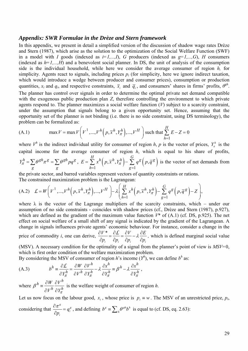
Appendix: SWR Formulae in the Drèze and Stern framework In this appendix, we present in detail a simplified version of the discussion of shadow wage rates Drèze and Stern (1987), which arise as the solution to the optimization of the Social Welfare Function (SWF) in a model with I goods (indexed as i=1,...,I), G producers (indexed as g=1,...,G), H consumers (indexed as h=1,...,H) and a benevolent social planner. In DS, the unit of analysis of the consumption side is the individual household, while here we consider the average consumer of region h, for simplicity. Agents react to signals, including prices pi (for simplicity, here we ignore indirect taxation, which would introduce a wedge between producer and consumer prices), consumption or production quantities, xi and qi, and respective constraints, ix and iq , and consumers’ shares in firms’ profits, θgh.

The planner has control over signals in order to determine the optimal private net demand compatible with the exogenous public production plan Z, therefore controlling the environment to which private agents respond to. The planner maximizes a social welfare function (V) subject to a scarcity constraint, under the assumption that signals belong to a given opportunity set. Hence, assuming that the opportunity set of the planner is not binding (i.e. there is no side constraint, using DS terminology), the problem can be formalized as:

(A.1) 1max max ,..., , , ,...,h h h HV V V V p x Y V

such that1

0H

hE Z

where Vh is the indirect individual utility for consumer of region h, p is the vector of prices, hY is the

capital income for the average consumer of region h, which is equal to his share of profits,

h gh g gh g

g gY pq ,

1 1, , ,

H Gh h h g g

h gE x p x Y q p q

is the vector of net demands from

the private sector, and barred variables represent vectors of quantity constraints or rations. The constrained maximization problem is the Lagrangean:

(A.2) 1

1 1,..., , , ,..., , , ,

H Gh h h H h h h g g

h gW V V p x Y V x p x Y q p q Z

L ,

where λ is the vector of the Lagrange multipliers of the scarcity constraints, which – under our assumption of no side constraints - coincides with shadow prices (cf., Drèze and Stern (1987), p.927), which are defined as the gradient of the maximum value function V* of (A.1) (cf. DS, p.925). The net effect on social welfare of a small shift of any signal is indicated by the gradient of the Lagrangean. A change in signals influences private agents’ economic behaviour. For instance, consider a change in the

price of commodity i, one can derive, *

i i i i

V V E

p p p p

L, which is defined marginal social value

(MSV). A necessary condition for the optimality of a signal from the planner’s point of view is MSV=0, which is first order condition of the welfare maximization problem. By considering the MSV of consumer of region h’s income (Yh), we can define bh as:

(A.3) h h h

h hh h h h h

W V x xb

Y V Y Y Y

L,

where h

hh h

W V

V Y

is the welfare weight of consumer of region h.

Let us now focus on the labour good, x , whose price is p w . The MSV of an unrestricted price, pi,

considering that g

gi

i

qp

, and defining g gh h

hb b is equal to (cf. DS, eq. 2.63):

30

(A.4) .

gh h gh h

h h g

h h g g

h g

x qx b

w w w w

x qx b q

w w

L

In other words, at the optimum, we can breakdown the MSV of a price change in the direct welfare effect on consumers (first term of A.4), the social value of extra profits changes (second term of A.4), and the social cost of meeting the induced change in net demands (third term of A.4). Again adopting the DS framework to our simplified setting, the marginal social value of the constrained

labour demand by consumer of region h, hx , can be defined as (cf. DS, eq. 2.67):

(A.5) h h

h h h hW V x

x V x x

L.

In other words, the marginal social of the labour supply constraint is given by the direct effect on welfare of marginal supply of labour, corrected by a change in the labour demand, which is the social cost of allowing this additional labour supply. Finally, the marginal social value of an increase in the constrained labour demand (negative supply) by firms is obtained by deriving the Lagrangean with respect to the ration hq , which using the notation

introduced before is (cf. DS, eq. 2.65):

(A.6) g g

h ghh g g

h

qb

q q q

L.

The first term in (A.6) shows how the effect of an increase in labour is distributed based on the vectors of property shares θ and of distributive coefficients b. The second term is the social value (evaluated at shadow prices) of the increase in labour supply. We shall now turn our attention to the four labour market structures identified in Section 3, and provide formal derivations in the DS setting of the main equations in the text.

a) Fairly Socially Efficient case (FSE)

In the FSE case the market for labour is competitive, hence wage is the market clearing variable. Using the Slutsky decomposition of consumer demands in income and substitution effects, where x̂ is compensated demand, (A.4) can be re-written as:

ˆgh h gh h

h g

x x x qb x x b q x

w w wY Y

L,

which, assuming that labour supply is fixed (hence, compensated consumer demands are inelastic with respect to w, implying that ˆ 0 x w ), leads to:

(A.7) gh h g

h g

qb x b q

w w

L

.

Let us now define the marginal social product as, g gj

j

gj

qS

wM P

q

w

,21 allowing us to

write:

21 In the main text we use m as a symbol for MSP.

31

.

gj

jg j

ggj

jg g j

gj

g

j gg j

gg

g

qqq

w w w

qq

w w

qqw

q ww

qMSP

w

Setting the MSV (A.7) of labour price equal to zero, we isolate the Lagrange multiplier for labour, ,

obtaining the SWR for the Fairly Socially Efficient (FSE) case:

(A.8)

gh h g

h ggFSE FSE

g

b x b q

SWR MSPq w

.

The SWR is equal to the marginal social product of labour plus a distributive term. The numerator of the second term of the SWR ( h h g g

h g

b x b q ) reflects distributional effects of a raise in wages due to the

creation of new employment.

b) Quasi-Keynesian Unemployment (QKU)

This labour market is characterized by involuntary unemployment, and clears by rationing of supply because wages are set under the reservation wage (for rationed household demand functions, see Neary and Roberts, 1980). Additional employment in this case requires a release of an additional unit of labour supply, i.e. a reduction in hx (by standard convention, labour supply is negative consumption of leisure

in x plans, and labour demand is negative supply in q plans).

Interpreting equation (A.5) in terms of the constraint demand of leisure, hx , the first term on the right

hand side of (A.5) is the social value of accepting a new job in the presence of Keynesian

unemployment and is the weighted difference between the reservation wage hwr (which can be thought

of as the disutility of labour in money terms) and the wage rate w . Hence, (A.5) can also be written (cf. DS, eq. 2.83), as:

hhjh h

w l jh h hj

xxr w

x x x

L,

which, defining h hj jh

j h h

x xw

x Y

the pure substitution effect of a small change in consumer of region

h’s ration of labour on his net demand for the generic good j, and recognizing that h hx x =1, and

equating (A.5) to zero leads us to write:

h hj jh h h h h h h

w j j w j jh hj j j

x xr w w r w

Y Y

.

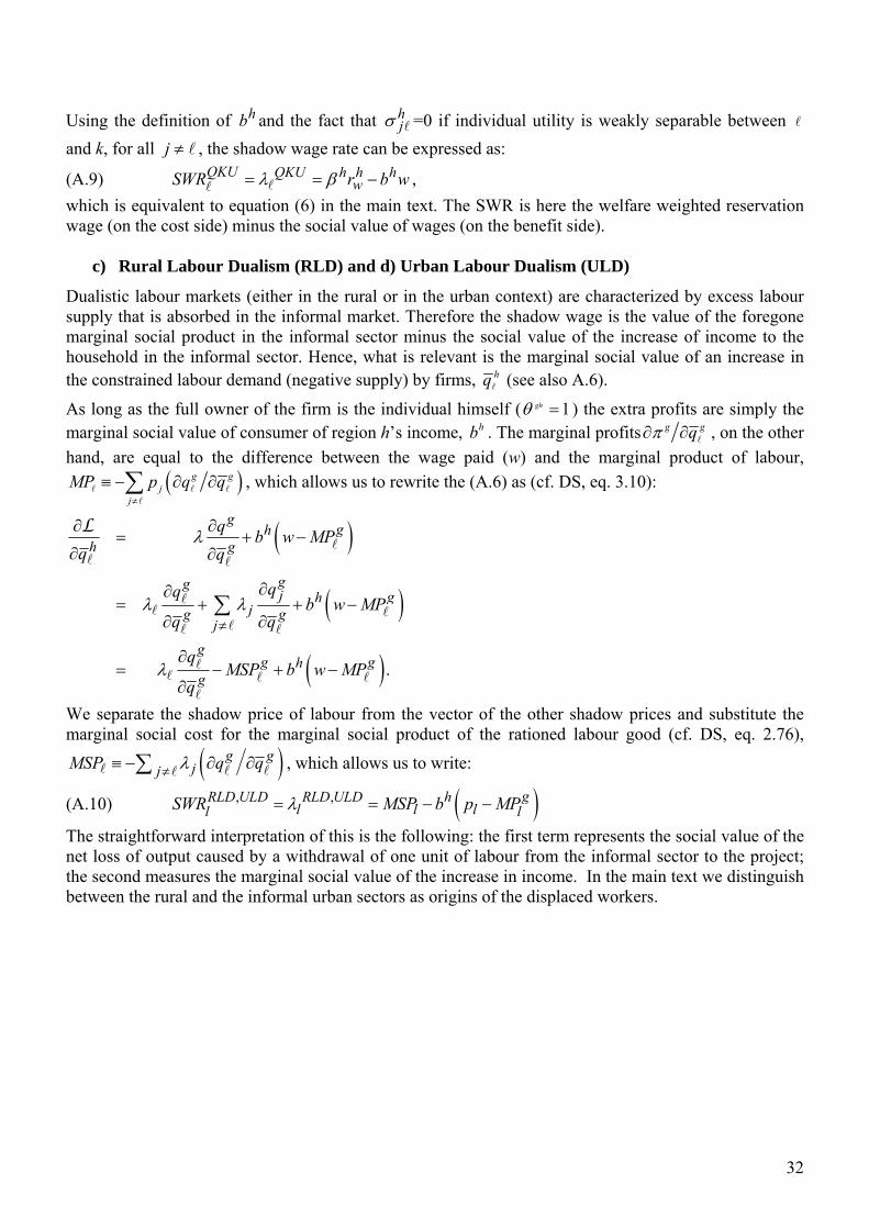
32

Using the definition of hb and the fact that hj =0 if individual utility is weakly separable between

and k, for all j , the shadow wage rate can be expressed as:

(A.9) QKU QKU h h hwSWR r b w ,

which is equivalent to equation (6) in the main text. The SWR is here the welfare weighted reservation wage (on the cost side) minus the social value of wages (on the benefit side).

c) Rural Labour Dualism (RLD) and d) Urban Labour Dualism (ULD)

Dualistic labour markets (either in the rural or in the urban context) are characterized by excess labour supply that is absorbed in the informal market. Therefore the shadow wage is the value of the foregone marginal social product in the informal sector minus the social value of the increase of income to the household in the informal sector. Hence, what is relevant is the marginal social value of an increase in the constrained labour demand (negative supply) by firms, hq (see also A.6).

As long as the full owner of the firm is the individual himself ( 1gh ) the extra profits are simply the marginal social value of consumer of region h’s income, hb . The marginal profits g gq , on the other

hand, are equal to the difference between the wage paid (w) and the marginal product of labour,

g gj

j

MP p q q

, which allows us to rewrite the (A.6) as (cf. DS, eq. 3.10):

.

ggh

h g

ggj gh

jg g

gg

g

j

gh

qb w MP

q q

qqb w MP

q q

qMSP b w MP

q

L

We separate the shadow price of labour from the vector of the other shadow prices and substitute the marginal social cost for the marginal social product of the rationed labour good (cf. DS, eq. 2.76),

g gjjMSP q q , which allows us to write:

(A.10) , , gRLD ULD RLD ULD hl l ll lSWR MSP b p MP

The straightforward interpretation of this is the following: the first term represents the social value of the net loss of output caused by a withdrawal of one unit of labour from the informal sector to the project; the second measures the marginal social value of the increase in income. In the main text we distinguish between the rural and the informal urban sectors as origins of the displaced workers.