j ourna l homepage: www.e lsev ie r .com/ locate /desa l
Shale gas flowback water desalination: Single vs multiple-effectevaporation with vapor recompression cycle and thermal integration
Viviani C. Onishi a,⁎, Alba Carrero-Parreño a, Juan A. Reyes-Labarta a, Rubén Ruiz-Femenia a,Raquel Salcedo-Díaz a, Eric S. Fraga b, José A. Caballero a
a Department of Chemical Engineering, University of Alicante, Ap. Correos 99, 03080 Alicante, Spainb Centre for Process Systems Engineering, Department of Chemical Engineering, University College London, London WC1E 7JE, UK
H I G H L I G H T S
• New NLP model for the SEE/MEE systems design including MVR and thermal integration• SEE/MEE model application to the high-salinity shale gas flowback water treatment.• Optimization by minimizing costs to achieve brine salinity close to ZLD conditions.• Sensitivity analysis to assess the system performance in distinct feed salinities• Results highlight the model accuracy to cost-effectively synthesize SEE/MEE systems.
Article history:Received 24 May 2016Received in revised form 26 September 2016Accepted 4 November 2016Available online xxxx
This paper introduces a new optimization model for the single and multiple-effect evaporation (SEE/MEE) sys-tems design, including vapor recompression cycle and thermal integration. The SEE/MEE model is specially de-veloped for shale gas flowback water desalination. A superstructure is proposed to solve the problem,comprising several evaporation effects coupled with intermediate flashing tanks that are used to enhance ther-mal integration by recovering condensate vapor.Multistage equipmentwith intercooling is used to compress thevapor formed by flashing and evaporation. The compression cycle is driven by electricity to operate on the vapororiginating from the SEE/MEE system, providing all the energy needed in the process. Themathematicalmodel isformulated as a nonlinear programming (NLP) problemoptimized under GAMS software byminimizing the totalannualized cost. The SEE/MEE system application for zero liquid discharge (ZLD) is investigated by allowing brinesalinity discharge near to salt saturation conditions. Additionally, sensitivity analysis is carried out to evaluate theoptimal process configuration and performance under distinct feed water salinity conditions. The results high-light the potential of the proposed model to cost-effectively optimize SEE/MEE systems by producing freshwater and reducing brine discharges and associated environmental impacts.
Natural gas extracted from tight shale formations or “shale gas”, isexpected to play an important role in meeting the rising global energydemand. In the U.S., it is estimated that natural gas production fromshale deposits will increase from 35% in 2012 to 50% in 2035 [1,2].This prediction is supported by the rapid progress achieved in recentyears in horizontal drilling and hydraulic fracturing technology, whichhas enhanced technically and economically the exploration of extensiveshale formations around North America [3–5]. In fact, the current ad-vances in shale gas production have significantly altered theworldwide
pq.cnpq.br (V.C. Onishi).
. This is an open access article under
energy scenario for any foreseeable future [6,7]. In Europe, shale gas ex-ploration has emerged as an attractive energy source mainly due itssupply reliability. Contrarily to petroleum-based energy sources, naturalgas production from unconventional reservoirs like shale deposits doesnot depend of unstable foreign markets that often dictate elevatedprices.
Natural gas production from shale formations requires well stimula-tion for starting andmaintaining the process, due to the low gas perme-ability on the rock [8,9]. Hence, the wells must be drilled and fracturedto retrieve the tight gas trapped in the shale rock formations. For thisreason, shale gas production consists of an unconventional gas drillingtechnology that requires large amounts ofwater for hydraulic fracturingof each well [10]. The fracturing fluids are injected into the horizontalwell under high pressure creating a complex artificial fracture network
the CC BY-NC-ND license (http://creativecommons.org/licenses/by-nc-nd/4.0/).
231V.C. Onishi et al. / Desalination 404 (2017) 230–248
to promote gas exhaustion. Usually, six or more wells are drilled hori-zontally through an extension of up to 2000 m, with a fracture networkdepth that can reach 500 m into the shale formation [11].
Actually, the development of technologies for drilling and hydrofracturing of shale gas plays are strongly conditioned by thewater avail-ability and flowback water disposal [5,12]. Recent studies estimate thatthe hydraulic fracturing of one single horizontal well demands approx-imately 3–6 million gallons of water (10,500–21,500 m3) [13,14]. Thehydraulic fracturing fluid is predominantly composed by water andsand (∼98%) containing several chemicals such as corrosion inhibitors,surfactants, friction reducers, acids, flow improvers [3]. Approximately10–80% of the amount of injected fluid flows back to surface duringthe first two weeks from the beginning of well exploitation [11,15].Along with the chemical additives utilized for fracturing the wells,flowback water also contains high concentrations of salts and otherminerals. Table 1 presents average and maximum values achieved forthe flowback water salinity from important U.S. shale plays, expressedin terms of the total dissolved solids (TDS). The flowback water can berecovered for recycling as injection water or for other purposes, de-manding specific treatment before any disposal and/or reuse.
Several works have been dedicated to the design and operation ofshale gas supply chains for optimal water management [1,4,16–19].Other studies have focused on the minimization of water consumption[5,13] and gaseous emissions [3,20] during shale gas production. How-ever, available literature about the treatment of high-salinity flowbackwater is scarce. It is worth noting that the water produced from shalegas drilling and fracturing can represent a serious environmental prob-lem, due to high concentrations of TDS and other pollutants.
The great potential of shale gas production at global scale highlightsthe need to develop more cost-effective processes for the treatment ofthe shale gas flowback water. Shaffer et al. [21] have critically reviewedpromising technologies for desalination of high-salinity producedwaterfrom shale gas exploration. According to the authors, mechanical vaporrecompression (MVR) systems are often more advantageous thanmembrane-based technologies for water desalination [22]. MVR sys-tems require less extensive pretreatment processes because they areusually less susceptible to fouling problems caused by the presence ofgrease and oil.
There are several publications addressing the optimization problemofmultiple-effect evaporation (MEE) systems. The first references in thefield date from 1840, with the MEE system being one of the oldest andmost widely used water desalination process around the globe [23].Halil and Söylemez [24] have developed a mathematical modeling ap-proach for the design and simulation of MEE processes for seawater de-salination, considering forward feed configuration and renewableenergy sources. Gautami and Khanam [25] have proposed nonlinearprogramming (NLP) models for MEE synthesis and optimization. Theoptimal design configuration is chosen according to the steam economyin the process. In the work of Druetta et al. [26], a nonlinear mathemat-ical model based on energy and mass balances is presented to predict
Table 1Flowback water salinity from different U.S. shale plays expressed in terms of total dis-solved solids (TDS).
Report U.S. Shale play TDS, ppm
Average Maximum
Acharya et al. [12] Fayetteville 13 k 20 kWoodford 30 k 40 kBarnett 80 k N150 kMarcellus 120 k N280 kHaynesville 110 k N200 k
Hayes [63]Haluszczak et al. [15] Marcellus 157ka 228ka
Thiel and Lienhard [69] Marcellus 145 k –Jiang et al. [70] Marcellus – 261 k
a TDS values for the flowback water in 14th day of hydraulic fracturing.
the optimal MEE performance in terms of energy efficiency. The MEEmodel is successfully applied to seawater desalination, and the sensitiv-ity analysis and simulations show good accuracy with realistic designs.Posteriorly, the model has been extended in Druetta et al. [27] to deter-mine the equipment capacity and operational conditions by consideringthe minimization of process costs as the objective function. Al-Mutazand Wazeer [28] have proposed mathematical models to evaluate theperformance of distinct configurations of conventionalMEE systems, in-cluding forward, backward and parallel/cross feed. More recently, Al-Mutaz [23] has published a comparative study on different seawater de-salination plants. His work indicates power consumption efficiency asthe main feature for making the MEE process more attractive than thedominant multistage flash (MSF) [29–32] and reverse osmosis (RO)[33–38] desalination processes. Piacentino [39] has introduced an in-depth cost analysis for multiple-effect distillation plants, through thecalculation of exergetic efficiency at subcomponent levels. His study in-troduces some key considerations when developing thermo-economi-cal models.
EI-Dessouky et al. [32,40–44] have made important contributions inmathematical modeling and design of MEE systems with/without me-chanical (MVR) or thermal vapor recompression (TVR). In EI-Dessoukyet al. [40], different models are presented for MEE systems design in-cluding MVR and TVR for seawater desalination. Mathematical modelsfor optimizing single-effect evaporation (SEE) systemswithmechanicalvapor recompression can be found in several studies in the literature[44–52]. Al-Juwayhel [45] have developed a comprehensive designmodel for the design of SEE includingMVR process. The model has pos-teriorly been expanded by Ettouney [44] for determining the geometri-cal characteristics of the evaporator, in addition to the heat transfer areaand power consumption calculations. The optimization of SEE systemswith MVR using mathematical programming has also been studied byMussati et al., [53] considering several non-convex constraints. Never-theless, it should be underlined that all of the above-mentioned workswere applied only to seawater desalination. Therefore, in previous stud-ies no considerations have beenmade about the treatment of very con-centrated feed and achievement of zero liquid discharge (ZLD) of brine.
ZLD systems have been studied by Thu et al. [54], by considering anadvanced multiple-effect adsorption process. The desalination processis developed to efficiently deal with high-salinity feed water, includingbrine from other seawater desalination plants. Chung et al. [55] havealso investigated ZLD application for the desalination of highly concen-tratedwater by allowing brine discharge close to NaCl saturation condi-tions. In their work, an approach based on finite differences is used tonumerically simulate a multistage membrane distillation process. Al-though the process can represent an attractive alternative over usualthermal desalination systems due to scale facility, by analyzingexergetic and energetic process efficiencies, the authors have concludedthat the required specific membrane area will determine its economicviability.
To surpass the aforementioned limitations, we introduce a newmathematical programming model for optimizing single and multiple-effect evaporation (SEE/MEE) systems, including vapor recompressioncycle and thermal integration. The SEE/MEE process is conceived forthe treatment of high-salinity flowback water originated during shalegas hydraulic fracturing process. The main objective of the proposedSEE/MEE system is to produce fresh water and concentrated salineclose to ZLD, considering the outflow brine salinity near to salt satura-tion conditions. For this purpose, the multiple-effect superstructure forflowback water desalination includes as many evaporation effects asthere are flashing tanks, placed intermittently. As a result, process ener-gy efficiency is further enhanced by recuperating the condensate vapor.The evaporation system is designedwith a counter-current flow config-uration. Thus, concentrated brine is recovered in the first evaporator ef-fect, while feed water is added to the last one after preheating. Inaddition, the vapor formed by evaporation and condensate flashing iscompressed through multistage electric-driven mechanical equipment
232 V.C. Onishi et al. / Desalination 404 (2017) 230–248
containing intercoolers. Consequently, the SEE/MEE process does notrequire any other external energy source.
The superstructure is mathematically formulated as an NLPmodel solved using GAMS, minimizing the total annualized cost of theprocess. The SEE and MEE optimal configurations including vaporrecompression cycle and heat integration are compared in terms oftheir ability to achieve ZLD conditions for the brine concentrate. Sensi-tivity analysis is performed to assess the optimal evaporation processconfiguration and performance under different flowback water salin-ities. In addition, the obtained results are validated by simulationsusing Aspen HYSYS software.
The main novelties introduced by this work include: (i) develop-ment of a more comprehensive and robust NLP model for the optimalsimultaneous synthesis of SEE/MEE systems, including vaporrecompression cycle and thermal integration; (ii) application of thepro-posed SEE/MEEmodel to the treatment of high-salinity flowbackwater,originating from the hydraulic fracturing process in shale gas produc-tion; (iii) SEE/MEE model application to ZLD conditions of the concen-trated brine and the high recovery ratio of fresh water; (iv) capabilityof the SEE/MEE model to effectively deal with very high concentrationsof the feed water; and, (v) facility of process scaling.
This paper is structured as follows: Section 2 presents the formalproblem statement, wherein the study boundaries are defined and themajor process features are described in detail. In Section 3, we developthe mathematical NLP model for the simultaneous SEE/MEE synthesis.The capabilities of our developed SEE/MEE model are evaluated inSection 4, by applying it to a case study based on shale gas production.In addition, this section shows the main results and discussions aboutthe sensitivity analysis and HYSYS simulations, and themost importantcomputational aspects. Finally, the conclusions of thework are present-ed in Section 5.
2. Problem statement
Given is a high-salinity flowback water stream from shale gas pro-duction, with a known supply state (inlet mass flowrate, salinity, tem-perature and pressure) and target specification defined by the brineconcentration. Additionally, equipment (for promoting heat exchange,evaporation, compression and separation) and energy services (includ-ing cooling water and electric power) are also provided, with their re-spective costs. The goal is to identify the optimal SEE/MEE systemconfiguration, considering the vapor recompression cycle and thermalintegration, by minimizing the process total annualized cost. The opti-mal process configuration should achieve a high recovery ratio offreshwater produced and brine close to the ZLD condition. The objectivefunction is composed of the capital cost of investment in equipment andthe operating expenses related to cold utility and electricity.
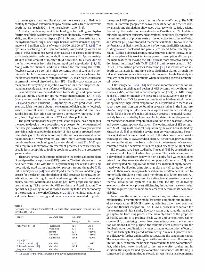
It should be highlighted that improving the process cost-effective-ness through the reduction of brine discharges (i.e., achieving ZLD con-ditions and consequently, increasing the fresh water production),allows lessening the environmental impacts associated to energy con-sumption and waste disposal. Shale gas exploration is a recent technol-ogy that requires further development, particularly in the framework ofthe flowback water treatment. To the best of our knowledge, this is thefirst work proposing the ZLD application to the treatment of theflowback water from shale gas fracking, through a SEE/MEE system in-cluding MVR and thermal integration. The multiple-effect superstruc-ture proposed for the desalination of shale gas flowback water isshowed in Fig. 1.
The following equipment are considered in the MEE system withvapor recompression and thermal integration:
(i) Shell-and-tube preheater (for the heat exchange between feedwater and condensate).
(ii) Multiple-effect evaporator.(iii) Multistage electricity-driven compressor with intercoolers.
(iv) Flashing tanks.(v) Pumps and mixers.
The MEE system comprises i evaporation effects intermediatelycoupled to flashing tanks that are used to recover condensate vapor, en-hancing process energy efficiency. Note that the SEE system corre-sponds to a simplification of the MEE process, being composed of asingle-effect evaporator without a flash tank. In this case, vapor flashingis not allowed due to the low amount of recoverable energy from thecondensate, which makes unfeasible the capital cost related to the allo-cation of such equipment.
In the proposed MEE system, the evaporation effects are numberedaccording to the direction of the heat flow (i.e., from 1 to i). The evapo-rator effect i is composed of the shell containing droplet separator (toremove water from the saturated vapor), spaces for the saturatedvapor and saline pool, brine spray nozzles and evaporation/condensa-tion tubes. A counter-current flow configuration is considered suchthat the vapor from the last evaporation effect and the condensatevapor from the last flash tank are compressed, through a mechanicalequipment composed by j stages. Thus, the superheated compressedvapor is added in the first evaporation effect, whereas the feed water(corresponding to the shale gas flowback water) is inserted in the lastone. It should be noted that the vapor recompression process is cyclic.Thus, the entire amount of vapor formed in the last evaporator effectis routed to themechanical vapor compressor together with the flashedoff condensate vapor from last flash tank —to be superheated to a de-sired target condition— before being added to the first evaporation ef-fect. It should be emphasized that the vapor recompression cycleallows further enhancing heat integration in evaporation systems, be-cause it operates on all the vapor originated from the evaporation sys-tem, providing the energy required in the process [56].
Under this system configuration, the first evaporation effect shouldpresent the highest temperature and pressure, while the last effect ishould be subjected to the lowest conditions for these variables. More-over, the vapor formed in the system follows the direction of droppingpressure (and temperature). The brine (feed) flows in the opposite di-rection. The superheated vapor from compression (for effect 1), aswell as the vapor formed in previous effects (for effects 2 to i), are intro-duced inside the evaporator tubes. The feed water (i.e., brine from sub-sequent stages for effects 1 to i-1; and, shale gas flowbackwater in effecti) is sprayed on the tubes in the shell-side to promote evaporation. Inthis way, the vapor is condensed on the tube-side by transferring its la-tent heat to the falling film formed by the sprayed feed. Observe that inthe first effect, the formed falling film outside tubes absorbs the latentheat from the compressed vapor starting the process of feed (i.e., brinefrom effect 2) evaporation. The vapor formed is used to drive effect 2.This process occurs successively until last effect i. Still in effect 1, sensi-ble heat is responsible for the temperature change in the tube-side,wherein the condensed vapor changes from the inlet superheatedvapor temperature to its desired outlet condition. Note that the conden-sate outlet temperature should correspond to the inlet vapor saturationpressure.
After each evaporation effect, the condensed vapor is sent to flashtanks to reduce its pressure (and temperature) and, consequently, re-cover energy. The small amount of flashed off condensate vapor in an ef-fect i, plus the vapor formed by boiling in the previous effect are addedto the tube-side of the subsequent evaporation effect. For this reason,both streams should be at the same pressure. Before entering into theevaporator, the feedwater is preheated taking in advantage the sensibleheat from the condensed vapor (i.e., produced fresh water) to improveheat integration in the evaporation system [57]. The increase in thefeed temperature is essential for improving the energy recovery andmaintaining the system productivity in the presence of climatic changesthroughout the year.
The SEE/MEE synthesis with MVR and thermal integration is acomplex process and we seek the optimal system configuration
Fig. 1.Multiple-effect evaporation superstructure proposed for the desalination of high-salinity flowback water from shale gas fracking.
233V.C. Onishi et al. / Desalination 404 (2017) 230–248
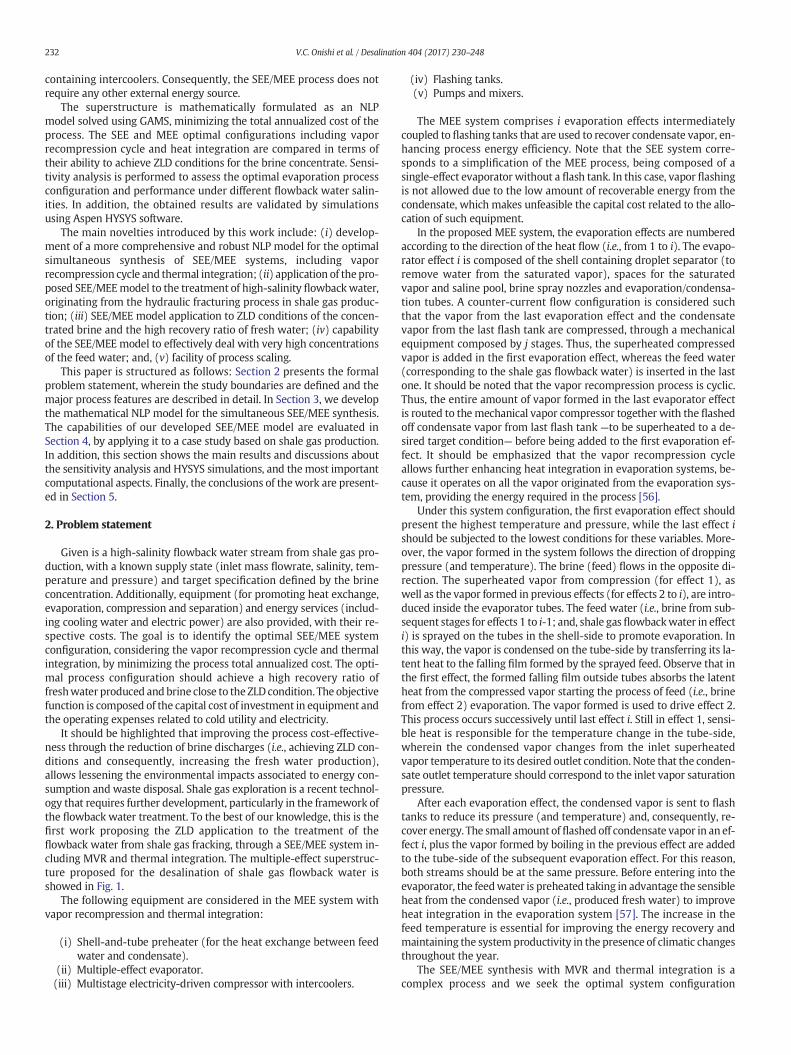
corresponding to lower heat transfer area and minimum services con-sumption (including thermal utilities and electricity). For this purpose,all flows properties (i.e., temperature, pressure, specific enthalpy, con-centration and flowrate) are unknown variables needing optimization.Fig. 2 (a) shows the main process variables for the effect i of the
Fig. 2. Process decision variables for (a) the effect i of the evapor
evaporator andflash tank i, while Fig. 2 (b) displays the systemvariablesfor the stage j of compression. Moreover, the elevated number of tem-perature constraints to guarantee the optimal equipment functioning,allied to the high non-convexity and nonlinearity of the cost correla-tions further increase the complexity of the model.
ator and flash tank i; and, (b) the stage j of the compressor.
234 V.C. Onishi et al. / Desalination 404 (2017) 230–248
For the desalination of the shale gas flowback water, it is assumedthat the feed water has been previously treated to remove all contami-nants, including chemical additives (such as flow improvers, acids, sur-factants, friction reducers, and corrosion inhibitors), oils, greases andsand. Water pretreatment technologies can include filtration, chemicaland physical precipitation, sedimentation and flotation. However, theshale gas flowbackwater still has high TDS concentration after pretreat-ment. The objective of the proposed SEE/MEE system is to supply, incombination with suitable water pretreatment technologies, highcost-effective recovery of fresh water for reuse or for safe disposal.Also, the system should operate at lowpressure and temperature to pre-vent equipment instability and avoid corrosion and fouling problems,which can be caused by the high salt concentration and the presenceof remaining oils and greases. In addition, the lower operation temper-atures allow for reducing process scaling and thermodynamic losses,allowing for minimal thermal insulation [41,43].
Due to the use of an electric-drivenmechanical compressor, the SEE/MEE system does not require an external energy source. An energy gen-erator can be used when electricity services are not available, makingthe SEE/MEE process suitable for use in remote off-grid locations.Other advantages of the SEE/MEE system include the consideration ofhorizontal tube configuration, in which the falling film formed allowsfor higher heat transfer coefficients and lower heat transfer areas [58].This reduces the capital costs of investment and equipment size,makingthe processmore compact and thereforemore easily transported.More-over, the MEE system permits the simple inclusion of additional evapo-ration effects due to its modular feature.
The following assumptions are considered to simplify the mathe-matical formulation:
(vi) Steady state operation.(vii) Heat losses in all thermal and mechanical equipment are
neglected.(viii) The non-equilibrium allowance (NEA) is neglected.(ix) Pressure drops in all thermal and mechanical equipment are
neglected.(x) Zero salinity for the condensate (product).(xi) Vapor streams fromeach evaporator effect behave as ideal gases.(xii) All effects of the evaporator are built with nickel (to avoid corro-
sion).(xiii) The multi-stage compressor is centrifugal (without drivers)
built with carbon steel.(xiv) Starter energy required for the multi-stage compressor is
neglected.(xv) Effect of surging and choking is disregarded in the multi-stage
compressor.(xvi) The vapor multi-stage compression is isentropic.(xvii) Shell-and-tube preheater and flash tanks are built with carbon
steel.(xviii) Capital costs of pumps and mixers are negligible.
The mathematical formulation of the proposed model includingequality and inequality constraints for the optimal SEE/MEE processsynthesis is presented in the following section.
3. Mathematical programming model
Themathematical programmingmodel for optimizing SEE/MEE sys-tems is formulated based on the superstructure presented in Fig. 1. Theproposed superstructure is composed by i evaporation effects coupledintermediately to i flashing tanks, and j compression stages. The inlettemperature (Tinfeed_water), mass flowrate (Finfeed_water) and salt concentra-tion (Sinfeed_water) of the feed water (i.e., shale gas flowback water) areknown parameters for themodel. The outlet conditions of the producedfresh water—including temperature (Toutfresh_water) and flowrate
(Foutfresh_water)—are variables that must be optimized by consideringbrine salinity specifications (Soutbrine). All intermediate streams tempera-tures (T), pressures (P), specific enthalpies (H), salt concentrations (S)and mass flowrates (F), as well as the system performance characteris-tics (including compression workW, heat transfer area A and heat flowQ) are decision variables requiring optimization. The mathematicalmodel formulation comprises mass and energy balances on all equip-ment and mixing points, and design constraints involving stream tem-peratures and pressures to avoid solutions without physical meaning.The objective function accounts for the total annualized process cost,which is composed by operational expenses and capital investment.The resulting NLP-based model is developed in the next sections, inwhich the SEE/MEE superstructure is generated according to the follow-ing steps.
3.1. Sets definition
The following sets are required to develop the NLP model.
I ¼ i=i is an evaporator effectf gJ ¼ j= j is a compression stagef g
Note that the number of evaporation effects and compression stagescan be chosen arbitrarily. However, the selection of larger values forthese indiceswill increases theproblem size and complexity and, conse-quently, the difficulty in obtaining a solution.
3.2. Multiple-effect evaporator
The multiple-effect evaporator design is as follows.
3.2.1. Evaporator mass balancesFor effects 1 to i-1, the feedwater corresponds to the brine from sub-
sequent effects at Fi+1brine and Si+1
brine conditions. In the last effect i, the feedstream is the shale gas flowback water to be treated (under Fifeed_water
and Sinfeed_water conditions). Thus, the mass balances for the effect i-1 of
Observe that for thefirst effect, the salinity of the brine should corre-spond to its outlet specification Sout
brine. In this study, we consider thebrine outlet specification near to salt saturation concentration toachieve zero liquid discharge conditions. For the last evaporation effect,the mass and salt balances are:
Ffeed wateri ¼ Fbrinei þ Fvapori i ¼ I ð3Þ
Ffeed wateri � Sfeed water
in ¼ Fbrinei � Sbrinei i ¼ I ð4Þ
3.2.2. Ideal temperatureThe ideal temperature Tiideal is defined as the temperature that an ef-
fect i should have if its brine salinity is equal to zero. The ideal temper-ature in effect i is estimated by Eq. (5).
ln Pvapori
� � ¼ aþ b= Tideali þ c
� �∀i∈I ð5Þ
The values for the Antoine parameters a, b and c in the Eq. (5) are12.98437,−2001.77468 and 139.61335, respectively. These correlationparameters have been obtained from HYSYS-OLI process simulator byconsidering the temperature in a range of 10≤Ti≤120oC and salt mass
235V.C. Onishi et al. / Desalination 404 (2017) 230–248
fractions XSibrine between 0 and 0.3, under the electrolytes thermody-namic package.
3.2.3. Boiling point elevation (BPE)The boiling point elevation (BPE) corresponds to the increase in the
boiling point temperature caused by the brine salt concentration. TheBPE is calculated as a function of the salt mass fraction (XSibrine) andthe ideal temperature (Tiideal) in an evaporation effect i.
3.2.4. Brine temperatureThe brine temperature (Tibrine) in an evaporation effect i should be
equal to its BPE added to its ideal temperature (Tiideal). In fact, thebrine temperature is considered to be the effect temperature. Thus,the brine and outlet vapor in an effect i (Tivapor) should be at the sametemperature Ti
brine.
Tbrinei ¼ Tideal
i þ BPEi ∀i∈I ð8Þ
3.2.5. Evaporator energy balancesThe overall energy balance for effect i should include the heat flows
added to the system boundary from feed water and condensed vapor,and the vapor and brine energy outflows. The overall energy balancesin each effect of the evaporator is given by Eq. (9) and Eq. (10).
Qevaporatori þ Fbrineiþ1 � Hbrine
iþ1 ¼ Fbrinei � Hbrinei þ Fvapori � Hvapor
i ibI ð9Þ
Qevaporatori þ Ffeed water
i � Hfeed wateri ¼ Fbrinei � Hbrine
i þ Fvapori � Hvapori i
¼ I ð10Þ
For which the specific enthalpies of the vapor, brine and feed water(i.e., shale gas flowback water) streams are estimated by the followingcorrelations:
As mentioned before, the vapor and brine streams are at the sametemperature Ti
brine in effect i. However, the specific enthalpy estimationfor the brine and for feedwater in the last effect should also consider theinfluence of their salinity in addition to the temperature.
3.2.6. Heat requirements in the evaporatorIn the first evaporation effect, the term Qi
evaporator in the Eq. (9) com-prises the latent heat needed to condense the superheated vapor fromthe compressor, and the sensible heat required to achieve the targetcondensate temperature (Ticondensate).
Qevaporatori ¼ Fspvi � Cpvapor � Tspv
j −Tcondensatei
� �þ Fspvi
� Hcvi −Hcondensate
i
� �i ¼ 1; j ¼ J
ð14Þ
In Eq. (14), Cpvapor is the specific heat for the vapor stream. In thiswork, it is considered to be constant in order to simplify the model.Tispv and Ti
condensate are the superheated vapor and condensate tempera-tures, respectively. The condensate temperature Ti
condensate is estimatedby considering the outlet compressor pressure Pj
spv in Antoine equationgiven by Eq. (5). Moreover,Hi
cv andHicondensate are the specific enthalpies
for the vapor and liquid phases of the condensate, respectively. Thesevariables are estimated by Eq. (11) and Eq. (12), considering the outletcondensate temperature Ti
condensate. Note that the salt mass fraction inEq. (12) should be equal to zero for the liquid specific enthalpy estima-tion. The variable Fi
spv indicates the superheated vapor flowrate, whichincludes the vapor flowrates from the last evaporator effect and flashingtank:
Fspv1 ¼ Fvapori þ Fvaporci i ¼ I ð15Þ
For effects 2 to i, the heat requirements include the contributions ofthe vaporization latent heat added by the boiling vapor, and the flashedoff condensate vapor from previous effect. The heat flows in each evap-oration effect are given by the following equation.
Qevaporatori ¼ Fvapori−1 � λi þ Fvaporci−1
� λi iN1 ð16Þ
In Eq. (16), Fi−1vapor and Fci−1
vaporare the boiling vapor and flashed offcondensate vapor flowrates from the previous effect, respectively. Thelatent heat of vaporization λi is calculated by the following correlation:
λi ¼ 2502:5−2:3648 � Tsvi þ 1:840 Tsv
i−1−Tsvi
� �iN1 ð17Þ
In which Tisv is the saturated vapor temperature estimated by Eq. (5)
corresponding to the saturated vapor pressure Pisv.
3.2.7. Feasibility of pressure and temperature between evaporator effectsThe outlet vapor pressure throughout the different effects of the
evaporator should decrease monotonically. Moreover, the outlet vaporpressure Pivapor in effect i should be equal to the saturated vapor pressurefrom the following effect i + 1 to avoid instabilities in the equipment.
Pvapori ≥Pvapor
iþ1 þ ΔPmin ibI ð18Þ
Pvapori ¼ Psv
iþ1 ibI ð19Þ
3.2.8. Overall heat transfer coefficient. The overall heat transfer coefficientUievaporator is estimated using the correlation presented by Al-Mutaz and
Wazeer [28].
Uevaporatori ¼ 0:001 � 1939:4þ 1:40562 � Tbrine
i −0:00207525 � Tbrinei
� �2þ 0:0023186 � Tbrine
i
� �3� �
ð20Þ
3.2.9. Evaporator heat transfer area. The evaporator is designed to be acompact piece of equipment composed of several evaporation effects.For this reason, a total heat transfer area should be determined for esti-mating costs. The total heat transfer area of the evaporator effects (Ai-evaporator) is given by Eq. (21).
Aevaporator ¼XI
i¼1
Ai ¼XI
i¼1
Qi= Ui � LMTDið Þ ð21Þ
In the first effect of the evaporator, the heat transfer area should beequal to the sum of the sensible and latent heat transfer areas. For thecalculation of the transfer area for sensible heat, the overall heat transfer
236 V.C. Onishi et al. / Desalination 404 (2017) 230–248
coefficient US is considered as a known parameter.
Ai ¼ A1i þ A2
i i ¼ 1 ð22Þ
A1i ¼ Fspvi � Cpvapor � Tspv
j −Tcondensatei
� �= US � LMTDi
� �i ¼ 1; j ¼ J ð23Þ
A2i ¼ Fspvi � Hcv
i −Hcondensatei
� �=Ui � Tcondensate
i −Tbrinei
� �i ¼ 1 ð24Þ
In order to avoid numerical difficulties related to matching temper-ature differences, Chen's approximation [59] is used to determine thelogarithmic mean temperature difference (LMTDi).
For obtaining amore uniformarea distribution, the following restric-tions are considered:
Ai≤n � Ai−1 iN1 ð27Þ
Ai≥Ai−1 iN1 ð28Þ
In which n is set to be equal to 3. However, it should be noted thatthe parameter n can be chosen arbitrarily according to the designerneed. If necessary, the constraint can be easily removed from themodel.
3.2.10. Temperature constraintsConstraints on temperature must be used to avoid temperature
crossovers in the evaporator effects. These constraints are defined bythe Eqs. (29)–(36).
Tspvj ≥Tcondensate
i þ ΔT1min i ¼ 1; j ¼ J ð29Þ
Tbrinei−1 ≥Tcondensate
i þ ΔT1min iN1 ð30Þ
Tbrinei ≥Tbrine
iþ1 þ ΔTstagemin ibI ð31Þ
Tbrinei ≥Tfeed
i þ ΔT2min i ¼ I ð32Þ
Tcondensatei ≥Tbrine
iþ1 þ ΔTmin ibI ð33Þ
Tcondensatei ≥Tfeed
i þ ΔTmin i ¼ I ð34Þ
Tcondensatei ≥Tbrine
i þ ΔTmin i∈I ð35Þ
Tsvi ≥Tbrine
i þ ΔTmin i∈I ð36Þ
3.3. Condensate flashing tanks
The condensate flashing tanks are modeled using the followingequations.
3.3.1. Mass balances in the flashing tank iThe mass balances in each flash tank i are given by the equations:
Fspvi ¼ Fvaporci þ Fliquidci i ¼ 1 ð37Þ
Fvapori−1 þ Fvaporci−1þ Fliquidci−1
¼ Fvaporci þ Fliquidci iN1 ð38Þ
In which Fcivapor and Fci
liquid are the mass flowrates for the flashed offvapor and liquid phases of the condensate, respectively.
3.3.2. Energy balances in the flashing tank iThe energy balances in each flash tank i are given by the equations:
Fspvi � Hcondensatei ¼ Fvaporci � Hvapor
ci þ Fliquidci � Hliquidci i ¼ 1 ð39Þ
Fvapori−1 þ Fvaporci−1
� �� Hcondensate
i þ Fliquidci−1� Hliquid
ci−1
¼ Fvaporci� Hvapor
ciþ Fliquidci
� Hliquidci
iN1 ð40Þ
In whichHicondensate andHci
liquid are the liquid specific enthalpies esti-mated by the Eq. (12) considering the temperatures of condensate Ti-condensate and ideal Tiideal, respectively. In both cases, salt mass fractionequal to zero (i.e., XSibrine=0) is assumed in Eq. (12). The specific enthal-py for the flash off vapor Hci
vapor from the condensate is obtained by Eq.(11), considering the ideal temperature in the effect.
3.3.3. Volume of the flashing tank iThe volume of each flashing tank i is given by the following equa-
tions:
Vflashi ¼ Fspvi � t� �
=ρ i ¼ 1 ð41Þ
Vflashi ¼ Fvapori−1 þ Fliquidci−1
� �� t=ρ iN1 ð42Þ
In which t indicates the retention time of the condensate inside theflash tank, and ρ the water density. In this study, a retention timeequal to 5 min is considered for flashing tanks design.
3.4. Condensate/feed preheater
The condensate/feed preheater used to heat the feed water is de-signed using the following equations.
3.4.1. Energy balance in the condensate/feed preheaterThe energy balance in the preheater is given by Eq. (43).
Fliquidci� Cpcondensatei � Tideal
i −Tfresh waterout
� �¼ Ffeed water
in � Cpfeedin � Tfeed wateri −Tfeed
in
� �i ¼ I ð43Þ
In which Tinfeed is the inlet feed temperature of the shale gas flowback
water. Cpicondensate and Cpinfeed are the specific heats of the condensate (i.e.,
fresh water produced) and feed water, respectively. The liquid specificheats are estimated by the following correlations:
Cpfeedin ¼ 0:001 �4206:8−6:6197 � Sfeed water
in þ 1:2288e−2 � Sfeed waterin
� �2� �
þ
−1:1262þ 5:418e−2 � Sfeed waterin
� �� Tfeed
in
264
375 i ¼ I
ð44Þ
Cpcondensatei ¼ 0:001 � 4206:8−1:1262 � Tideali
� �i ¼ I ð45Þ
237V.C. Onishi et al. / Desalination 404 (2017) 230–248
3.4.2. Heat transfer area of the condensate/feed preheaterThe heat transfer area Apreheaterof the condensate/feed preheater is
determined by the equation:
Apreheater ¼ Fliquidci � Cpcondensatei � Tideali −Tfresh water
out
� �=Upreheater
�LMTDpreheater i ¼ I
ð46Þ
In which, the overall heat transfer coefficient Upreheater is estimatedby Eq. (20) considering the ideal temperature Ti
idealfor the last evapora-tor effect. In this case, the log mean temperature difference (LMTD-preheater) is calculated by Eq. (25), with the temperature difference inthe hot and cold terminals given by:
θpreheater1 ¼ Tideali −Tfeed water
i i ¼ I and θpreheater2
¼ Tfresh waterout −Tfeed
in ð47Þ
3.5. Multistage mechanical compressor
Themultistagemechanical compressorwith intercooling is designedusing the following mathematical formulation.
3.5.1. Heat dutyThe amount of heat Qj
cooler exchanged by the intercooler is given byEq. (48).
Qcoolerj ¼ Fspvi � Cpvapor � Tspv
j−1−Tcj
� �jN1 ð48Þ
In which Tj−1spv is the inlet temperature in the intercooler that should
correspond to the compressor outlet temperature from the previousstage. On the other hand, Tjc is the intercooler outlet temperature,which should be equal to the inlet temperature in the next compressionstage.
3.5.2. Constraints on intercoolers temperaturesConstraints are necessary to ensure that the outlet temperature from
an intercooler is lower than the correspondent inlet temperature on it(i.e., the vapor stream should be cooled):
Tspvj−1≥T
cj þ ΔTcooler
min jN1 ð49Þ
Note that the outlet intercooler temperature should be above thesaturation temperature in order to avoid the presence of liquid in thecompressor, and related operational issues.
3.5.3. Energy balance in the mixerAn energy balance is needed in the mixer allocated before the com-
pressor, to guarantee that the inlet vapor temperature in such equip-ment is at mixture temperature Ti
m.
Fvaporci Tmi −Tideal
i
� �¼ Fvapori � Tbrine
i −Tmi
� �i ¼ I ð50Þ
3.5.4. Isentropic temperatureThe isentropic temperature of the compressed/superheated vapor is
given by the equations:
Tisj ¼ Tm
i þ 273:15� � � Pspv
j =Pvapori
� �γ−1=γ−273:15 i ¼ I; j ¼ 1 ð51Þ
Tisj ¼ Tc
j þ 273:15� �
� Pspvj =Pspv
j−1
� �γ−1=γ−273:15 jN1 ð52Þ
Inwhichγ is theheat capacity ratio. The outlet pressure of the super-heated vapor Pjspv in the stage j should be limited to a maximum com-pression ratio:
Pspvj ≤CRmax � Pvapor
i i ¼ I; j ¼ 1 andPspvj ≤CRmax � Pspv
j−1 jN1 ð53Þ
3.5.5. Temperature of the superheated vaporThe superheated vapor temperature, i.e. the compressor outlet tem-
perature in the stage j is calculated by the equation:
Tspvj ¼ Tc
j þ 1=η � Tisj −Tc
j
� �∀ j∈ J ð54Þ
In which η is the isentropic efficiency of the compressor.
3.5.6. Constraints on compressor temperatures and pressuresIn the compression stage j, an increase of the vapor temperature and
pressure is expected:
Tspvj ≥Tc
j ∀ j∈ J ð55Þ
Pspvj ≥Pvapor
i i ¼ I; j ¼ 1 ð56Þ
Pspvj ≥Pspv
j−1 jN1 ð57Þ
3.5.7. Compression workThe total compression work is expressed in terms of the enthalpies
difference of the compressed superheated vaporHjspv and the inlet com-
pressor vapor Hjc in each stage j:
W ¼XJ
j¼1
W j ¼XJ
j¼1
Fspvi � Hspvj −Hc
j
� �i ¼ 1 ð58Þ
InwhichHjspv andHj
c are the specific enthalpies for the vapor streamsestimated by Eq. (11), considering the inlet (Tjc) and outlet (Tjspv) com-pressor temperatures, respectively. For allowing a more uniform com-pression capacities distribution, the following restrictions areconsidered:
W j≤m �W j−1 jN1 ð59Þ
W j≥W j−1 jN1 ð60Þ
In whichm is set to be equal to 3. The parameterm can be chosen ar-bitrarily according to the designer specification. Note that the equip-ment is more expensive as higher uniformity is required for thecompressor construction. If necessary, the constraint can be easily re-moved from the model.
3.6. Design specification
To achieve the ZLD condition, the brine salinity at first effect shouldbe at least equal to its design specification.
Sbrinei ≥Sbrineout i ¼ 1 ð61Þ
All correlations presented in themathematical formulation—includ-ing the correlations for estimation of the BPE (Eq. (6)), liquid and vaporspecific enthalpies (Eq. (11)–(13)), latent heat of vaporization (Eq.(17)); and, liquid specific heat (Eq. (44) and Eq. (45)) — have been ob-tained fromHYSYS-OLI simulator by using the thermodynamic packagefor electrolytes, and considering salt mass fractions between 0 and 0.30.
Table 2Problem data for the case study based on the shale gas production.
Feed water (shale gas flowback water)Mass flowrate 37.5 m3 h−1 (10.42 kg s−1)Salinity 70 g kg−1
Temperature 25 °CPressure 50 kPa
Multistage compressor with intercoolingType/material Centrifugal/carbon steelIsentropic efficiency 0.75Heat capacity ratio 1.33Maximum compression ratio 3 per stageCooling services temperature 20–25 °C
SpecificationsBrine salinity 300 g kg−1
Cost dataElectricity costa 850.51 US$ (kW year)−1
Cooling services cost 100 US$ (kW year)−1
Factor of annualized capital cost 0.16 (10% - 10 years)
a Data obtained from Eurostat [71] database for industrial consumers in EuropeanUnion (2015 - S1).
238 V.C. Onishi et al. / Desalination 404 (2017) 230–248
3.7. Objective function
The objective function corresponds to the minimization of the totalannualized cost of the SEE/MEE process with mechanical vaporrecompression and heat recovery. The objective function is defined bythe following mathematical formulation.
3.7.1. Total annualized costThe total annualized cost of the SEE/MEE system with mechanical
vapor recompression and thermal integration should be equal to thesum between capital costs (CAPEX) and operational expenses (OPEX)as described by Eq. (62).
TAC ¼ CAPEX þ OPEX ð62Þ
3.7.2. Total capital expendituresThe total capital costs CAPEX should account for the investment cost
of all equipment in the SEE/MEE system with mechanical vaporrecompression and thermal integration. Therefore, the calculation ofthe total capital cost includes the expenditures for the preheater, multi-ple-effect evaporator, multistage compressor and flashing tanks.
In which fac is the annualization factor for the capital cost as definedby Smith [60]:
fac ¼ r 1þ rð Þy1þ rð Þy−1
ð64Þ
In which r is the fractional interest rate per year and y is the numberof years (amortization period). In Eq. (63), CPO indicates the basic costof a unitary equipment (in kUS$) operating at pressure close to ambientconditions. CPO is estimated using the correlations presented by Turtonet al. [61] for the preheater and flashing tanks. For the cost estimation ofthe evaporator and the multistage compressor, the correlations pro-posed by Couper et al. [62] are considered. FBM corresponds to the fac-tor of correction for the basic unitary cost, in which the constructionmaterials and the operational pressure of these equipment units arecorrelated. Moreover, the total annualized cost must be corrected forthe relevant year using the CEPCI index (Chemical Engineering PlantCost Index).
3.7.3. Operational expendituresOperational expenditures comprise the electricity and cooling ser-
vices consumed by the multistage compressor:
OPEX ¼ Ec �XJ
j¼1
W j þ Cc �XJ
j¼1
Qcoolerj ð65Þ
In which Ec and Cc are the cost parameters for electricity and coolingservices, respectively.
4. Case study
A case study is performed to verify the accuracy of the proposedmathematical model for optimizing SEE/MEE systems, consideringvapor recompression cycle and thermal integration. It should behighlighted that the problem data used in this example are based on
real data obtained from important U.S. shale plays such as Marcellusand Barnett [63–66]. The capacity of the centralized treatment plantshould be 900 m3 day−1 (or 10.42 kg s−1) of shale gas flowbackwater. Interestingly, Lira-Barragán et al. [4] report in a recent workthat under an uncertain scenario as the amount of water required tocomplete each well (i.e., considering a standard deviation of 10% in theshale plays data), the choice of the aforementioned value(900m3 day−1) has 100% probability of guaranteeing that the plant ca-pacity is adequate to treat the total amount offlowbackwater. These au-thors have considered a mean value of 15 k m3 (in a range of 12–18 k m3) for the amount of water needed for the hydraulic fracturingof each well, from which 25% is expected to return to surface asflowback water during the first 3 weeks. Additionally, the total numberof wells to be treated is divided in fracturing crews following an annualscheduling capable for answering the hydraulic drilling of 20 wells peryear [4].
Typical salinity average values (measured as total dissolved solids -TDS) for the shale gas flowback water from the Marcellus play are re-ported in the literature in a range of 120–157 k ppm [12,15,63]. Howev-er, it should be mentioned that other U.S. shale plays can present verydistinct salt concentrations for the flowback water as shown in Table1. For this reason, an initial mean value of 70 k ppm (or 70 g kg−1) isconsidered for the feed salinity in the SEE/MEE system design. Never-theless, it should be noted that themodel is robust enough to guaranteeoptimal solutions for a large range of salinities and flowrates of theflowback water, underlining the facility for process scaling. Model per-formance and system sensitivity are evaluated under higher salinitiesin the next sections. Table 2 presents the problem data, while Fig. 1shows the general superstructure proposed for the desalination of thehigh-salinity flowback water from shale gas fracking.
Additional problem data include the minimum pressure and tem-perature drop between evaporator effects equal to 0.1 kPa and 0.1 °C, re-spectively.Moreover, theminimum temperature approach between theoutlet vapor and concentrated brine, as well as between the superheat-ed vapor (i.e., vapor after compression) and condensate (freshwater) inan evaporator effect is ΔTmin=2oC. The unknown minimum ideal tem-perature in the evaporation effect i is considered in a range of 1–100 °Cto avoid operational problems (including rusting and fouling), while thesaturated vapor pressure is restricted to 1–200 kPa. Most importantly,concentrate discharge salinity is specified to be equal to 300 g kg−1
(very close to salt saturation condition of ~350 g kg−1) in order toachieve ZLD operation. In the case study, a factor of annualized capitalcost (fac) of 0.16 is considered; this corresponds to 10% interest rateover a period of 10 years.
239V.C. Onishi et al. / Desalination 404 (2017) 230–248
4.1. Optimizing the SEE/MEE system configuration
Several SEE/MEE system configurations are evaluated for their cost-effectiveness in obtaining concentrated brine at ZLD conditions andfresh water. In all cases, the minimization of the total annualized costof the evaporation process is considered to be the objective function,which is composed by operational expenses and capital cost of invest-ment. Initially, the system is optimized considering multiple-effectevaporation (MEE) without any additional equipment. In this case,steam at 120 °C and 50 kPa provided from an external source—Cvapor=418.8 US$(year kW)‐1— is added to the first evaporation ef-fect. The counter-current flow configuration is considered: the feedwater (shale gas flowback water) is introduced in the last effect of theevaporator. In this way, the last evaporator effect is submitted to thelowest pressure and temperature of the system. The optimization oftheMEE process is carried out by varying the number of evaporation ef-fects. Thus, the optimal configuration obtained consists of 3 evaporatoreffects with heat transfer areas (and heat flow) equal to 204.16 m2
(7086.95 kW), 176.91 m2 (6896.88 kW) and 114.27 m2 (6159.42 kW),respectively. The total annualized cost (TAC) is equal to3237 k US$ year−1, comprising 2579 k US$ year−1 related to operatingexpenses (OPEX) and 658 k US$ year−1 to capital cost of investment(CAPEX). Note that the evaporator with 2 effects presents a TAC equalto 4557kUS$ year−1 (OPEX=4043kUS$ year−1 and CAPEX=514kUS$year−1) while the evaporation equipment with 4 effects has a total costof 4812 k US$ year−1 composed by OPEX=2205k US$ year−1 andCAPEX=2607k US$ year−1. Therefore, the operating costs related tothe consumed steam in the process is significantly reduced as the num-ber of effects is increased (~36% of reduction from 2 to 3 effects) in theevaporator. This fact is related to the increment in the total heat transferarea that reduces the amount of heat required in the equipment. Notethat, although the operational costs are decreasing with the increasingin the evaporator area, there is a threshold (3th effect) from that the
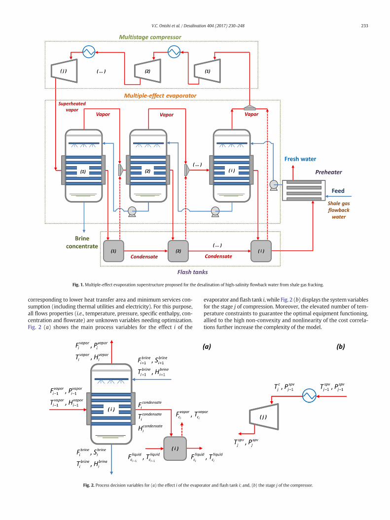
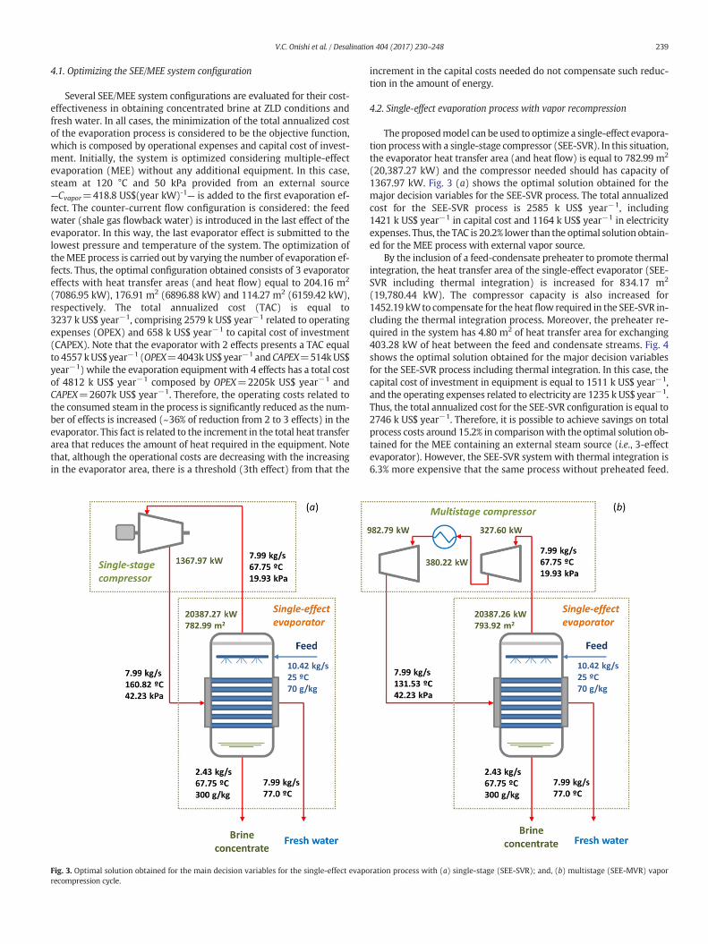
Fig. 3. Optimal solution obtained for the main decision variables for the single-effect evaporecompression cycle.
increment in the capital costs needed do not compensate such reduc-tion in the amount of energy.
4.2. Single-effect evaporation process with vapor recompression
The proposedmodel can be used to optimize a single-effect evapora-tion processwith a single-stage compressor (SEE-SVR). In this situation,the evaporator heat transfer area (and heat flow) is equal to 782.99 m2
(20,387.27 kW) and the compressor needed should has capacity of1367.97 kW. Fig. 3 (a) shows the optimal solution obtained for themajor decision variables for the SEE-SVR process. The total annualizedcost for the SEE-SVR process is 2585 k US$ year−1, including1421 k US$ year−1 in capital cost and 1164 k US$ year−1 in electricityexpenses. Thus, the TAC is 20.2% lower than the optimal solution obtain-ed for the MEE process with external vapor source.
By the inclusion of a feed-condensate preheater to promote thermalintegration, the heat transfer area of the single-effect evaporator (SEE-SVR including thermal integration) is increased for 834.17 m2
(19,780.44 kW). The compressor capacity is also increased for1452.19 kWto compensate for the heatflow required in the SEE-SVR in-cluding the thermal integration process. Moreover, the preheater re-quired in the system has 4.80 m2 of heat transfer area for exchanging403.28 kW of heat between the feed and condensate streams. Fig. 4shows the optimal solution obtained for the major decision variablesfor the SEE-SVR process including thermal integration. In this case, thecapital cost of investment in equipment is equal to 1511 k US$ year−1,and the operating expenses related to electricity are 1235 k US$ year−1.Thus, the total annualized cost for the SEE-SVR configuration is equal to2746 k US$ year−1. Therefore, it is possible to achieve savings on totalprocess costs around 15.2% in comparisonwith the optimal solution ob-tained for the MEE containing an external steam source (i.e., 3-effectevaporator). However, the SEE-SVR system with thermal integration is6.3% more expensive that the same process without preheated feed.
ration process with (a) single-stage (SEE-SVR); and, (b) multistage (SEE-MVR) vapor
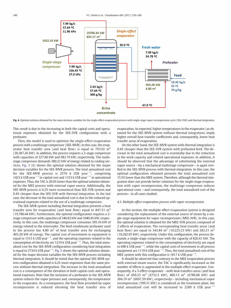
Fig. 4.Optimal solution obtained for themain decision variables for the single-effect evaporation process with single-stage vapor recompression cycle (SEE-SVR) and thermal integration.
240 V.C. Onishi et al. / Desalination 404 (2017) 230–248
This result is due to the increasing in both the capital costs and opera-tional expenses obtained for the SEE-SVR configuration with apreheater.
Then, the model is used to optimize the single-effect evaporationprocesswith amultistage compressor (SEE-MVR). In this case, the evap-orator heat transfer area (and heat flow) is equal to 793.92 m2
(20,387.26 kW). In addition, the process requires a 2-stage compressorwith capacities of 327.60 kW and 982.79 kW, respectively. The multi-stage compressor demands 380.22 kW of energy related to cooling ser-vices. Fig. 3 (b) shows the optimal solution obtained for the majordecision variables for the SEE-MVR process. The total annualized costfor the SEE-MVR process is 2576 k US$ year−1, comprising1423 k US$ year−1 in capital cost and 1153 k US$ year−1 in operationalexpenses. Thus, the TAC is 20.4% lower than the optimal solution obtain-ed for the MEE process with external vapor source. Additionally, theSEE-MVR process is 6.2% more economical than SEE-SVR system and0.4% cheaper than the SEE-SVR with thermal integration. In the lastcase, the decrease in the total annualized cost is due to the reduced op-erational expenses related to the use of a multistage compressor.
The SEE-MVR system including thermal integration presents a heattransfer area for evaporation (and heat flow) equal to 847.51 m2
(19,780.44 kW). Furthermore, the optimal configuration requires a 2-stage compressorwith capacities of 346.82 kWand1040.45 kW, respec-tively. In this case, the multistage compressor consumes 395.16 kW ofenergy related to the intercooler. The feed-condensate preheater usedin the process has 4.80 m2 of heat transfer area for exchanging403.28 kW of energy. The capital cost of investment in equipment isequal to 1515 k US$ year−1, and the operating expenses related to theconsumption of electricity are 1219 k US$ year−1. Thus, the total annu-alized cost for the SEE-MVR configuration considering heat integrationis equal to 2734 k US$ year−1. Fig. 5 shows the optimal solution obtain-ed for the major decision variables for the SEE-MVR process includingthermal integration. It should be noted that the optimal SEE-MVR sys-tem configuration obtained is 6.2% more expensive than the same pro-cess without thermal integration. The increase in the total annualizedcost is a consequence of the elevation in both capital costs and opera-tional expenses. Note that the inclusion of a preheater in the SEE-MVRsystem reduces the vapor pressure and, consequently, the temperaturein the evaporator. As a consequence, the heat flow provided by vaporrecompression is reduced elevating the heat transfer area of
evaporation. As expected, higher temperatures in the evaporator (as ob-tained for the SEE-MVR system without thermal integration) implyhigher overall heat transfer coefficients and, consequently, lower heattransfer areas of evaporation.
On the other hand, the SEE-MVR systemwith thermal integration is0.4% cheaper than the SEE-SVR system with preheated feed. The de-crease in the total annualized cost is essentially due to the reductionin the work capacity and related operational expenses. In addition, itshould be observed that the advantage of substituting the externalvapor source —by a mechanical multistage compressor— is again veri-fied in the SEE-MVR process with thermal integration. In this case, theoptimal configuration obtained presents the total annualized cost15.5% lower than theMEE system. Therefore, although the thermal inte-gration does not provide better solutions for the single-stage evapora-tion with vapor recompression, the multistage compressor reducesoperational costs —and consequently, the total annualized cost of theprocess— in all cases studied.
4.3. Multiple-effect evaporation process with vapor recompression
In this section, the multiple-effect evaporation system is designedconsidering the replacement of the external source of steam by a sin-gle-stage equipment for vapor recompression (MEE-SVR). In this case,the optimal solution is obtained for the MEE-SVR process composed of2 effects of evaporation. The corresponding heat transfer areas (andheat flow) are equal to 343.84 m2 (10,225.23 kW) and 282.21 m2
(10,262.95 kW), respectively. Under this configuration, the process de-mands a single-stage compressor with the capacity of 820.41 kW. Theoperating expenses related to the consumption of electricity are equalto 698 k US$ year−1, while the capital costs of investment in all processequipment are 1119 k US$ year−1. Thus, the total annualized cost of theMEE system with this configuration is 1817 k US$ year−1.
It should be observed that contrary to the MEE evaporation processwith external steam source, the TAC is significantly increased as thenumber of effects is augmented in the multiple-effect evaporator. Con-sequently, if a 3-effect evaporator —with heat transfers areas (and heatflow) of 450.23 m2 (6752.5 kW), 469.13 m2 (6780.68 kW) and304.19 m2 (6697.59 kW), respectively— including mechanical vaporrecompression (599.31 kW) is considered as the treatment plant, thetotal annualized cost will be increased to 2289 k US$ year−1
Fig. 5.Optimal solution obtained for the main decision variables for the single-effect evaporation process withmultistage vapor recompression cycle (SEE-MVR) and thermal integration.
241V.C. Onishi et al. / Desalination 404 (2017) 230–248
(OPEX=510k US$ year−1 and CAPEX=1779k US$ year−1). This valuecorresponds to an increment of 25.9% in relation to the TAC obtainedfor the design with 2 effects of evaporation. Note that the increase inthe total annualized cost is due to the need for bigger evaporator heattransfer areas, in which capital costs are significantly augmentedwhen considering three (~59% more expensive) or more evaporationeffects. On the other hand, the total annualized cost obtained consider-ing the MEE-SVR system with 2 evaporation effects (and single-stagecompressor) is 43.9% lower than the optimal solution found for thesteam-driven MEE process. This reduction in the total costs is possiblebecause, although a pressure manipulation equipment is used in theprocess —requiring an increased total heat transfer area of evapora-tion— the additional costs related to the inclusion in the MEE-SVR sys-tem of such mechanical compressor (including operational expensesand capital costs) do not exceed the expenses associated to externalsteam source (~270%more expensive than electricity expenses). More-over, the MEE-SVR process is 29.4% cheaper than the best solution ob-tained for the single-effect evaporation process (i.e., SEE-MVR withoutthermal integration). In this case, capital costs and operating expensesrelated to electricity consumption are both reduced when consideringthe multiple-effect evaporation process.
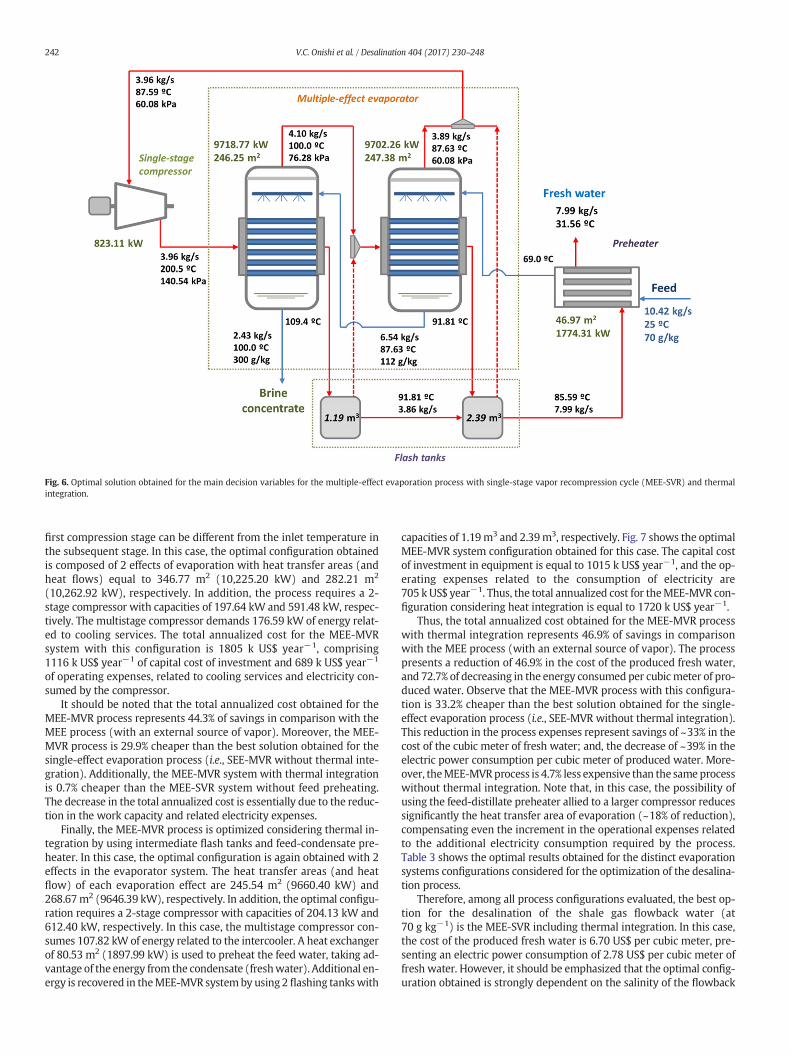
Afterwards, the MEE-SVR process is optimized considering thermalintegration through the inclusion of flash tanks and feed-condensatepreheater. In this case, the optimal configuration is again obtainedwith 2 effects in the evaporator. The heat transfer areas (and heatflow) of each evaporator effect are 246.25 m2 (9718.77 kW) and247.38 m2 (9702.26 kW), respectively. Moreover, a single-stage me-chanical compressorwith the capacity of 823.11 kW is needed formeet-ing the energy required in the process. In this case, thermal integrationis allowed in the process by using a preheaterwith area of 46.97m2 ableto exchange 1774.31 kW of heat between the fresh water (distillate)and the feed water. Additionally, 2 flashing tanks —with volumesequal to 1.19 m3 and 2.39 m3, respectively— are used to separate thedistillate vapor, providing a further energy recovery in the MEE-SVR
system. Fig. 6 shows the optimalMEE-SVRprocess configuration obtain-ed for this case study. The total annualized cost of the process with thisconfiguration is 1689 k US$ year−1, composed of 989 k US$ year−1 re-lated to capital cost of investment in equipment and 700 k US$ year−1
to operating expenses of electricity consumption. Note that, the processdesigned with 3 evaporation effects has a total annualized cost of1904 k US$ year−1, composed of OPEX=568k US$ year−1 andCAPEX=1336k US$ year−1. Therefore, analogously to the behavior ob-served for the MEE-SVR system without thermal integration, the pro-cess total annualized cost is significantly increased when moreevaporator effects are considered in the system.
It should be highlighted that theMEE-SVR process design with ther-mal integration is 38.5% cheaper than the SEE-SVR system withpreheating of the feed water. Moreover, the MEE-SVR process is 34.4%less expensive than thebest solution obtained for the single-effect evap-oration process (i.e., SEE-MVRwithout thermal integration). In addition,this MEE-SVR configuration (i.e., containing flash tanks and preheater)allows for reducing costs in 7.1%, comparing with the optimal solutionobtained for the MEE-SVR without heat integration; and, 47.8% whencompared with the optimal solution found for theMEE process. By ana-lyzing these results, it is possible to observe that the heat recovery in theMEE-SVR process reduces significantly the total heat transfer area(~21% of reduction) required in the evaporator, in comparison withthe MEE-SVR without thermal integration. The equipment size reduc-tion is responsible for the considerable decrease in the capital cost of in-vestment (~12% of reduction) and, subsequently, in the total annualizedcost. Therefore, the thermal integration associated with the vaporrecompression cycle in the MEE-SVR system is essential for enhancingenergy efficiency and, consequently, for reducing process costs.
After the single-stage compression step, the developed mathemati-cal model is used to optimize the multiple-effect evaporation system,considering multistage vapor recompression and thermal integration(MEE-MVR). Observe that the optimization is performed consideringno pressure drop in the intercooler, and the inlet temperature in the
Fig. 6. Optimal solution obtained for the main decision variables for the multiple-effect evaporation process with single-stage vapor recompression cycle (MEE-SVR) and thermalintegration.
242 V.C. Onishi et al. / Desalination 404 (2017) 230–248
first compression stage can be different from the inlet temperature inthe subsequent stage. In this case, the optimal configuration obtainedis composed of 2 effects of evaporation with heat transfer areas (andheat flows) equal to 346.77 m2 (10,225.20 kW) and 282.21 m2
(10,262.92 kW), respectively. In addition, the process requires a 2-stage compressor with capacities of 197.64 kW and 591.48 kW, respec-tively. The multistage compressor demands 176.59 kW of energy relat-ed to cooling services. The total annualized cost for the MEE-MVRsystem with this configuration is 1805 k US$ year−1, comprising1116 k US$ year−1 of capital cost of investment and 689 k US$ year−1
of operating expenses, related to cooling services and electricity con-sumed by the compressor.
It should be noted that the total annualized cost obtained for theMEE-MVR process represents 44.3% of savings in comparison with theMEE process (with an external source of vapor). Moreover, the MEE-MVR process is 29.9% cheaper than the best solution obtained for thesingle-effect evaporation process (i.e., SEE-MVR without thermal inte-gration). Additionally, the MEE-MVR system with thermal integrationis 0.7% cheaper than the MEE-SVR system without feed preheating.The decrease in the total annualized cost is essentially due to the reduc-tion in the work capacity and related electricity expenses.
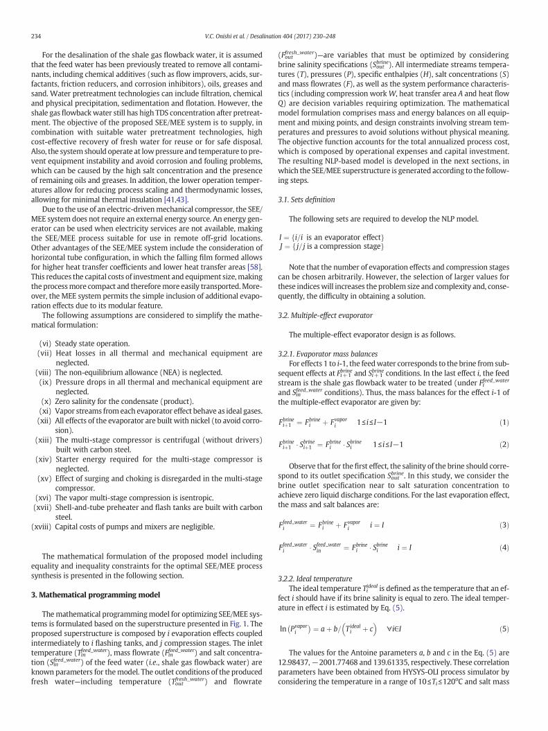
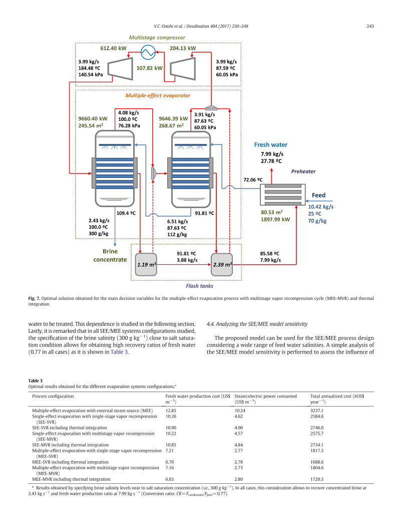
Finally, the MEE-MVR process is optimized considering thermal in-tegration by using intermediate flash tanks and feed-condensate pre-heater. In this case, the optimal configuration is again obtained with 2effects in the evaporator system. The heat transfer areas (and heatflow) of each evaporation effect are 245.54 m2 (9660.40 kW) and268.67m2 (9646.39 kW), respectively. In addition, the optimal configu-ration requires a 2-stage compressor with capacities of 204.13 kW and612.40 kW, respectively. In this case, the multistage compressor con-sumes 107.82 kW of energy related to the intercooler. A heat exchangerof 80.53 m2 (1897.99 kW) is used to preheat the feed water, taking ad-vantage of the energy from the condensate (freshwater). Additional en-ergy is recovered in theMEE-MVR systemby using 2 flashing tankswith
capacities of 1.19m3 and 2.39m3, respectively. Fig. 7 shows the optimalMEE-MVR system configuration obtained for this case. The capital costof investment in equipment is equal to 1015 k US$ year−1, and the op-erating expenses related to the consumption of electricity are705 k US$ year−1. Thus, the total annualized cost for theMEE-MVR con-figuration considering heat integration is equal to 1720 k US$ year−1.
Thus, the total annualized cost obtained for the MEE-MVR processwith thermal integration represents 46.9% of savings in comparisonwith the MEE process (with an external source of vapor). The processpresents a reduction of 46.9% in the cost of the produced fresh water,and 72.7% of decreasing in the energy consumed per cubicmeter of pro-duced water. Observe that the MEE-MVR process with this configura-tion is 33.2% cheaper than the best solution obtained for the single-effect evaporation process (i.e., SEE-MVR without thermal integration).This reduction in the process expenses represent savings of ~33% in thecost of the cubic meter of fresh water; and, the decrease of ~39% in theelectric power consumption per cubic meter of produced water. More-over, theMEE-MVRprocess is 4.7% less expensive than the sameprocesswithout thermal integration. Note that, in this case, the possibility ofusing the feed-distillate preheater allied to a larger compressor reducessignificantly the heat transfer area of evaporation (~18% of reduction),compensating even the increment in the operational expenses relatedto the additional electricity consumption required by the process.Table 3 shows the optimal results obtained for the distinct evaporationsystems configurations considered for the optimization of the desalina-tion process.
Therefore, among all process configurations evaluated, the best op-tion for the desalination of the shale gas flowback water (at70 g kg−1) is the MEE-SVR including thermal integration. In this case,the cost of the produced fresh water is 6.70 US$ per cubic meter, pre-senting an electric power consumption of 2.78 US$ per cubic meter offresh water. However, it should be emphasized that the optimal config-uration obtained is strongly dependent on the salinity of the flowback
Fig. 7. Optimal solution obtained for the main decision variables for the multiple-effect evaporation process with multistage vapor recompression cycle (MEE-MVR) and thermalintegration.
243V.C. Onishi et al. / Desalination 404 (2017) 230–248
water to be treated. This dependence is studied in the following section.Lastly, it is remarked that in all SEE/MEE systems configurations studied,the specification of the brine salinity (300 g kg−1) close to salt satura-tion condition allows for obtaining high recovery ratios of fresh water(0.77 in all cases) as it is shown in Table 3.
Table 3Optimal results obtained for the different evaporation systems configurations.a
Process configuration Fresh water productim−3)
Multiple-effect evaporation with external steam source (MEE) 12.85Single-effect evaporation with single-stage vapor recompression(SEE-SVR)
10.26
SEE-SVR including thermal integration 10.90Single-effect evaporation with multistage vapor recompression(SEE-MVR)
10.22
SEE-MVR including thermal integration 10.85Multiple-effect evaporation with single-stage vapor recompression(MEE-SVR)
7.21
MEE-SVR including thermal integration 6.70Multiple-effect evaporation with multistage vapor recompression(MEE-MVR)
7.16
MEE-MVR including thermal integration 6.83
a Results obtained by specifying brine salinity levels near to salt saturation concentration (i.2.43 kg s−1 and fresh water production ratio at 7.99 kg s−1 (Conversion ratio: CR=Fcondensate/F
4.4. Analyzing the SEE/MEE model sensitivity
The proposed model can be used for the SEE/MEE process designconsidering a wide range of feed water salinities. A simple analysis ofthe SEE/MEE model sensitivity is performed to assess the influence of
on cost (US$ Steam/electric power consumed(US$ m−3)
Total annualized cost (kUS$year−1)
10.24 3237.14.62 2584.6
4.90 2746.04.57 2575.7
4.84 2734.12.77 1817.3
2.78 1688.62.73 1804.6
2.80 1720.3
e., 300 g kg−1). In all cases, this consideration allows to recover concentrated brine atfeed=0.77).
244 V.C. Onishi et al. / Desalination 404 (2017) 230–248
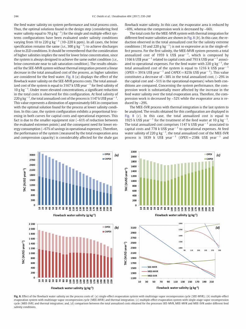
the feed water salinity on system performance and total process costs.Thus, the optimal solutions found in the design step (considering feedwater salinity equal to 70 g kg−1) for the single andmultiple-effect sys-tems configurations have been evaluated under salinity conditionsvarying from 10 to 220 g kg−1 (10–220 k ppm). In all cases, the brinespecification remains the same (i.e., 300 g kg−1) to achieve dischargesclose to ZLD conditions. It should be remembered that the considerationof higher salinities implies the need for lower brine concentration, sincethe system is always designed to achieve the same outlet condition (i.e.,brine concentrate near to salt saturation condition). The results obtain-ed for the SEE-MVR systemwithout thermal integration present a lineardecrease in the total annualized cost of the process, as higher salinitiesare considered for the feed water. Fig. 8 (a) displays the effect of theflowbackwater salinity on the SEE-MVRprocess costs. The total annual-ized cost of the system is equal to 3167 k US$ year−1 for feed salinity of10 g kg−1. Under more elevated concentrations, a significant reductionin the total costs is observed for this configuration. At feed salinity of220 g kg−1, the total annualized cost of theprocess is 1147 kUS$ year−1.This value represents a diminution of approximately 64% in comparisonwith the optimal solution found for the process at lower salinity condi-tion. In this case, the system configuration exhibits a proportional less-ening in both curves for capital costs and operational expenses. Thisfact is due to the smaller equipment size (~61% of reduction betweenthe evaluated extremes points) and the consequent need for lower en-ergy consumption (~67% of savings in operational expenses). Therefore,the performance of the system (measured by the total evaporation areaand compression capacity) is considerably affected for the shale gas
Fig. 8. Effect of the flowback water salinity on the process costs of: (a) single-effect evaporaevaporation system with multistage vapor recompression cycle (MEE-MVR) and thermal intcycle (MEE-SVR) and thermal integration; and, (d) comparison between the total annualizedsalinity conditions.
flowback water salinity. In this case, the evaporator area is reduced by~69%, whereas the compression work is decreased by ~66%.
The total costs for theMEE-MVR systemwith thermal integration fordifferent feedwater salinities are shown in Fig. 8 (b). In this case, the re-duction observed in the total annualized cost for the salinity extremeconditions (10 and 220 g kg−1) is not so expressive as in the single-ef-fect process. For the first salinity, the MEE-MVR system presents a totalannualized cost of 1959 k US$ year−1, which is composed by1166 k US$ year−1 related to capital costs and 793 k US$ year−1 associ-ated to operational expenses. For the feed water with 220 g kg−1, thetotal annualized cost of the system is equal to 1216 k US$ year−1
(OPEX=391k US$ year−1 and CAPEX=825k US$ year−1). This valueconstitutes a decrease of ~38% in the total annualized cost, (~29% inthe capital cost and ~51% in the operational expenses) when both con-ditions are compared. Concerning the system performance, the com-pression work is substantially more affected by the increase in thefeed water salinity over the total evaporation area. Therefore, the com-pression work is decreased by ~52% while the evaporator area is re-duced by ~29%.
The MEE-SVR process with thermal integration is the last system tobe analyzed. The results obtained for this configuration are displayed inFig. 8 (c). In this case, the total annualized cost is equal to1925 k US$ year−1 for the treatment of the feed water at 10 g kg−1.The total annualized cost comprises 1147 k US$ year−1 associated tocapital costs and 778 k US$ year−1 to operational expenses. At feedwater salinity of 220 g kg−1, the total annualized cost of the MEE-SVRprocess is 1839 k US$ year−1 (OPEX=238k US$ year−1 and
tion system with multistage vapor recompression cycle (SEE-MVR); (b) multiple-effectegration; (c) multiple-effect evaporation system with single-stage vapor recompressioncosts obtained for the processes SEE-MVR, MEE-MVR and MEE-SVR under different feed
245V.C. Onishi et al. / Desalination 404 (2017) 230–248
CAPEX=1601k US$ year−1). This value represents a reduction of ~5% incomparison with the optimal solution found for the process at10 g kg−1. The systemwith this configuration presents ~69% of savingsin operational expenses. On the other hand, the capital cost of invest-ment is increased by ~40%. This fact is due to the significant increasein the total evaporation area (~93%), whereas the compression workis reduced by ~70%. However, the MEE-SVR system configuration ex-hibits an inflection point at the feed water salinity equal to 80 g kg−1.Therefore, the process presents a minimum total annualized cost of1646 k US$ year−1 under this condition.
Finally, Fig. 8 (d) shows the comparison between the total annual-ized costs obtained for the processes SEE-MVR, MEE-MVR and MEE-SVR under different feed salinity conditions. In this figure, it is possibleto observe that the MEE-SVR process (with thermal integration) pre-sents the lower total costs at salinities between 10 and 100 g kg−1. Inthis concentration range, the SEE-MVR (without thermal integration)is the most expensive process for the treatment of the shale gasflowback water. Between the salinities of 100 to 150 g kg−1, the MEE-MVR system (with thermal integration) becomes the most economicalprocess to achieve brine discharges close to ZLD conditions. From salin-ities higher than 150 g kg−1, the MEE-SVR system is the less beneficialprocess. Note that the MEE-SVR system presents the lower comparedtotal annualized cost for the feed salinity at 70 g kg−1. Interestingly,the SEE-MVR system has the lower total annualized cost for salinitieshigher than 180 g kg−1. Observe that the SEE-MVR process is widelyused in the seawater desalination industry, in which there is no needto achieve ZLD conditions.
Fig. 9. MEE-MVR process flow diagram in Aspen HYSYS used t
4.5. Simulating the MEE process
To verify the accuracy of the proposed mathematical programmingmodel, a simulation of the process has been carried out using the com-mercial software Aspen HYSYS (version V8.8). With this aim, the MEE-MVR superstructure shown in Fig. 1 has been simulated consideringsteady state conditions. The resulting MEE-MVR process flow diagraminAspenHYSYS is displayed in Fig. 9. TheMEE-MVR systemhas been se-lected due to its elevated complexity in comparison with the other sys-tems designed.
The thermodynamic package NTRL-electrolytes has been chosen forthe process simulation. Moreover, the results obtained for the decisionvariables (i.e., inlet and outlet pressures and temperatures, and massflowrates) in the design step (shown in Fig. 7) have been introducedin the simulator to estimate the work capacities or heat flows of allequipment. A reasonably good agreement has been observed betweenthe design and simulated values for the MEE-MVR process. The simula-tion results showed that the compressor stages should have the capac-ities of 208.7 kWand 618.3 kW, respectively. In this case, the intercoolerconsumes 111.8 kW of energy. These values present differences of 0.9%,2.2% and 3.7%, respectively, in relation to the design ones. In the simula-tion, the effects of the evaporator present heat flows equal to 9555 kWand 9652 kW, respectively. The difference between the values obtainedfrom the model and the simulated ones are equal to 1.2% and 0.1%,respectively.
The simulation of the preheater has also shown high precision withthe modeled results. The difference between the two values is equal to
o validate the results obtained in the system design step.
246 V.C. Onishi et al. / Desalination 404 (2017) 230–248
0.8%. In this case, the heat duty simulated is equal to 1882 kW. More-over, all the remaining simulated values (including some inlet or outlettemperatures, pressures and mass flowrates) exhibit variations in rela-tion to the design values lower than 1%. It should be highlighted that thelow differences obtained between the modeling and simulation aremainly due to the use of correlations to estimate some decision vari-ables in the mathematical model.
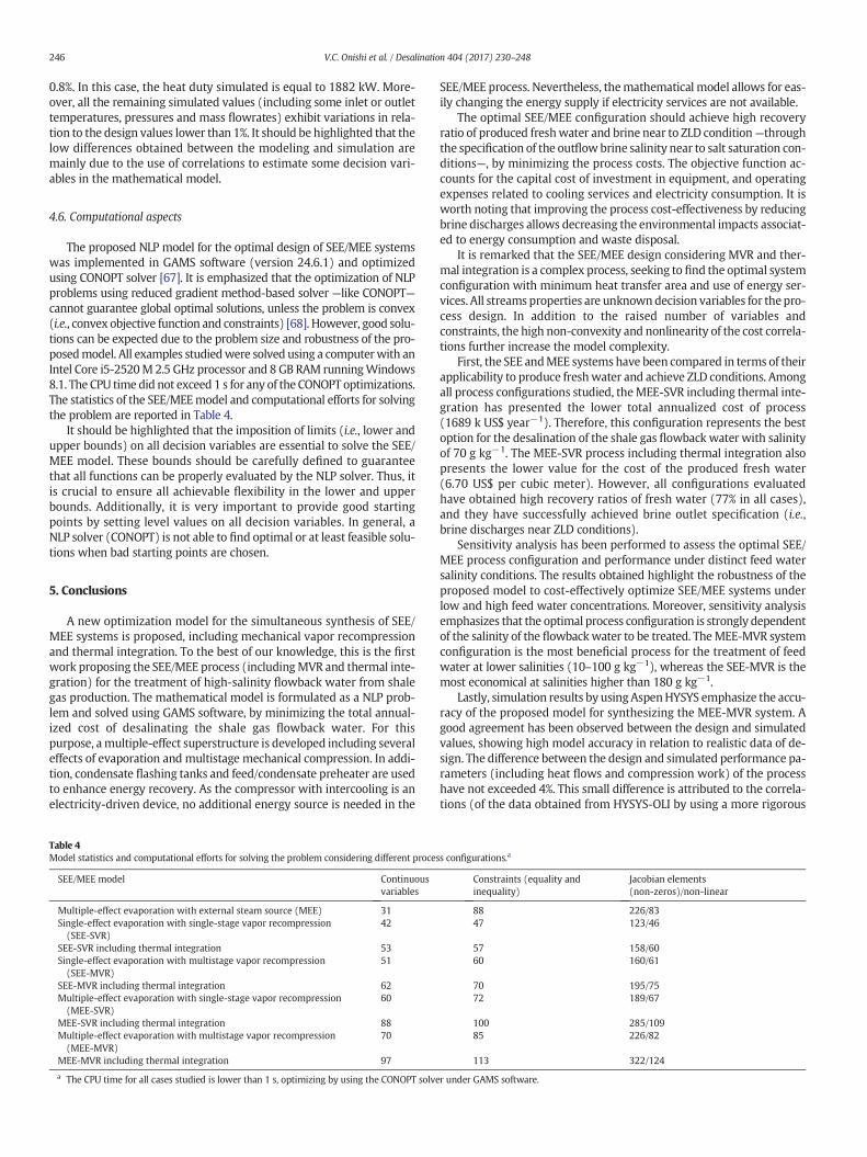
4.6. Computational aspects
The proposed NLP model for the optimal design of SEE/MEE systemswas implemented in GAMS software (version 24.6.1) and optimizedusing CONOPT solver [67]. It is emphasized that the optimization of NLPproblems using reduced gradient method-based solver —like CONOPT—cannot guarantee global optimal solutions, unless the problem is convex(i.e., convex objective function and constraints) [68]. However, good solu-tions can be expected due to the problem size and robustness of the pro-posedmodel. All examples studiedwere solved using a computerwith anIntel Core i5-2520M 2.5 GHz processor and 8 GB RAM runningWindows8.1. The CPU timedid not exceed 1 s for any of the CONOPT optimizations.The statistics of the SEE/MEEmodel and computational efforts for solvingthe problem are reported in Table 4.
It should be highlighted that the imposition of limits (i.e., lower andupper bounds) on all decision variables are essential to solve the SEE/MEE model. These bounds should be carefully defined to guaranteethat all functions can be properly evaluated by the NLP solver. Thus, itis crucial to ensure all achievable flexibility in the lower and upperbounds. Additionally, it is very important to provide good startingpoints by setting level values on all decision variables. In general, aNLP solver (CONOPT) is not able to find optimal or at least feasible solu-tions when bad starting points are chosen.
5. Conclusions
A new optimization model for the simultaneous synthesis of SEE/MEE systems is proposed, including mechanical vapor recompressionand thermal integration. To the best of our knowledge, this is the firstwork proposing the SEE/MEE process (includingMVR and thermal inte-gration) for the treatment of high-salinity flowback water from shalegas production. The mathematical model is formulated as a NLP prob-lem and solved using GAMS software, by minimizing the total annual-ized cost of desalinating the shale gas flowback water. For thispurpose, amultiple-effect superstructure is developed including severaleffects of evaporation and multistage mechanical compression. In addi-tion, condensate flashing tanks and feed/condensate preheater are usedto enhance energy recovery. As the compressor with intercooling is anelectricity-driven device, no additional energy source is needed in the
Table 4Model statistics and computational efforts for solving the problem considering different proces
SEE/MEE model Continuousvariables
Multiple-effect evaporation with external steam source (MEE) 31Single-effect evaporation with single-stage vapor recompression(SEE-SVR)
42
SEE-SVR including thermal integration 53Single-effect evaporation with multistage vapor recompression(SEE-MVR)
51
SEE-MVR including thermal integration 62Multiple-effect evaporation with single-stage vapor recompression(MEE-SVR)
60
MEE-SVR including thermal integration 88Multiple-effect evaporation with multistage vapor recompression(MEE-MVR)
70
MEE-MVR including thermal integration 97
a The CPU time for all cases studied is lower than 1 s, optimizing by using the CONOPT solve
SEE/MEE process. Nevertheless, themathematical model allows for eas-ily changing the energy supply if electricity services are not available.
The optimal SEE/MEE configuration should achieve high recoveryratio of produced freshwater and brine near to ZLD condition—throughthe specification of the outflowbrine salinity near to salt saturation con-ditions—, by minimizing the process costs. The objective function ac-counts for the capital cost of investment in equipment, and operatingexpenses related to cooling services and electricity consumption. It isworth noting that improving the process cost-effectiveness by reducingbrine discharges allows decreasing the environmental impacts associat-ed to energy consumption and waste disposal.
It is remarked that the SEE/MEE design considering MVR and ther-mal integration is a complex process, seeking to find the optimal systemconfiguration with minimum heat transfer area and use of energy ser-vices. All streams properties are unknowndecision variables for thepro-cess design. In addition to the raised number of variables andconstraints, the high non-convexity and nonlinearity of the cost correla-tions further increase the model complexity.
First, the SEE andMEE systems have been compared in terms of theirapplicability to produce freshwater and achieve ZLD conditions. Amongall process configurations studied, theMEE-SVR including thermal inte-gration has presented the lower total annualized cost of process(1689 k US$ year−1). Therefore, this configuration represents the bestoption for the desalination of the shale gas flowback water with salinityof 70 g kg−1. The MEE-SVR process including thermal integration alsopresents the lower value for the cost of the produced fresh water(6.70 US$ per cubic meter). However, all configurations evaluatedhave obtained high recovery ratios of fresh water (77% in all cases),and they have successfully achieved brine outlet specification (i.e.,brine discharges near ZLD conditions).
Sensitivity analysis has been performed to assess the optimal SEE/MEE process configuration and performance under distinct feed watersalinity conditions. The results obtained highlight the robustness of theproposed model to cost-effectively optimize SEE/MEE systems underlow and high feed water concentrations. Moreover, sensitivity analysisemphasizes that the optimal process configuration is strongly dependentof the salinity of the flowbackwater to be treated. TheMEE-MVR systemconfiguration is the most beneficial process for the treatment of feedwater at lower salinities (10–100 g kg−1), whereas the SEE-MVR is themost economical at salinities higher than 180 g kg−1.
Lastly, simulation results by usingAspenHYSYS emphasize the accu-racy of the proposed model for synthesizing the MEE-MVR system. Agood agreement has been observed between the design and simulatedvalues, showing high model accuracy in relation to realistic data of de-sign. The difference between the design and simulated performance pa-rameters (including heat flows and compression work) of the processhave not exceeded 4%. This small difference is attributed to the correla-tions (of the data obtained from HYSYS-OLI by using a more rigorous
s configurations.a
Constraints (equality andinequality)
Jacobian elements(non-zeros)/non-linear
88 226/8347 123/46
57 158/6060 160/61
70 195/7572 189/67
100 285/10985 226/82
113 322/124
r under GAMS software.
247V.C. Onishi et al. / Desalination 404 (2017) 230–248
thermodynamic package for electrolytes) used in the mathematicalmodel formulation.
Further development of the process technology is needed to ensurethe best possibilities for the treatment of the shale gas flowback water.Thus, future works include the study of the influence of the overall heattransfer coefficient on the process configuration and performance; anal-ysis of the uncertainty associated to the concentration data of thewells;and, consideration of the salinity variation as a function of the explora-tion time. Finally, the assessment of environmental impacts followingLCA principles should also be considered for the optimal design ofmore environmentally conscious processes.
Nomenclature
Roman letters
A heat transfer area, m2
BPE boiling point elevation, °CCAPEX capital expenses, kUS$ year−1
Cc cost parameter for the cooling services, US$ (kW year)−1
Cp specific heat, kJ (kg °C)−1
CPO cost of equipment unit, kUS$CRmax maximum compression ratioEc cost parameter for electricity, US$ (kW year)−1
fac factor of annualized capital costF mass flowrate, kg s−1
FBM correction factor for the capital costFP parameter for the capital cost estimationH specific enthalpy, kJ kg−1
LMTD logarithmic mean temperature differenceOPEX operational expenses, kUS$ year−1
P pressure, kPaΔPmin minimum pressure approach, kPaQ heat flow, kWr fractional interest rate per yearS salinity, g kg−1
T temperature, °Ct retention time in the flash tanks, minΔTmin minimum temperature approach, °CTAC total annualized cost, kUS$ year−1
U overall heat transfer coefficient, kW m−2 K−1
V volume, m3
XS Salt mass fractiony number of yearsW compression work, kW
Subscripts
c condensatei evaporator effectsj compressor stages
Superscript
c compressoris isentropicm mixturecv condensate vaporsv saturated vaporspv superheated vapor
Acronyms
CEPCI Chemical Engineering Plant Cost IndexGAMS General Algebraic Modeling SystemLCA Life Cycle AssessmentMEE Multiple-Effect EvaporationMSF Multistage FlashMVR Mechanical Vapor RecompressionNLP Nonlinear ProgrammingRO Reverse OsmosisSEE Single-Effect EvaporationTDS Total Dissolved SolidsTVR Thermal Vapor RecompressionZLD Zero Liquid Discharge
This project has received funding from the European Union'sHorizon 2020 Research and Innovation Programme under grant agree-ment No. 640979. The financial support provided by the NationalCouncil for Scientific and Technological Development of Brazil (CNPq),under process No. 233953/2014-0 is also gratefully acknowledged.
References
[1] J. Gao, F. You, Shale gas supply chain design and operations toward better economicand life cycle environmental performance: MINLPmodel and global optimization al-gorithm, ACS Sustain. Chem. Eng. 3 (2015) 1282–1291, http://dx.doi.org/10.1021/acssuschemeng.5b00122.
[2] B. Xiong, A.L. Zydney, M. Kumar, Fouling of microfiltration membranes by flowbackand produced waters from the Marcellus shale gas play, Water Res. (2016), http://dx.doi.org/10.1016/j.watres.2016.04.049.
[3] T. Stephenson, J.E. Valle, X. Riera-Palou,Modeling the relative GHG emissions of con-ventional and shale gas production, Environ. Sci. Technol. 45 (2011) 10757–10764,http://dx.doi.org/10.1021/es2024115.
[4] L.F. Lira-Barragán, J.M. Ponce-Ortega, G. Guillén-Gosálbez, M.M. El-Halwagi, Optimalwater management under uncertainty for shale gas production, Ind. Eng. Chem. Res.55 (2016) 1322–1335, http://dx.doi.org/10.1021/acs.iecr.5b02748.
[5] J.-P. Nicot, B.R. Scanlon, Water use for shale-gas production in Texas, U.S. Environ.Sci. Technol. 46 (2012) 3580–3586, http://dx.doi.org/10.1021/es204602t.
[6] C.L. Weber, C. Clavin, Life cycle carbon footprint of shale gas: review of evidence andimplications, Environ. Sci. Technol. 46 (2012) 5688–5695, http://dx.doi.org/10.1021/es300375n.
[7] M.S. Mauter, P.J.J. Alvarez, A. Burton, D.C. Cafaro, W. Chen, K.B. Gregory, G. Jiang, Q.Li, J. Pittock, D. Reible, J.L. Schnoor, Regional variation in water-related impacts of
248 V.C. Onishi et al. / Desalination 404 (2017) 230–248
shale gas development and implications for emerging international plays, Environ.Sci. Technol. 48 (2014) 8298–8306, http://dx.doi.org/10.1021/es405432k.
[8] A. Vengosh, N. Warner, R. Jackson, T. Darrah, The effects of shale gas exploration andhydraulic fracturing on the quality of water resources in the United States, ProcediaEarth Planet. Sci. 7 (2013) 863–866, http://dx.doi.org/10.1016/j.proeps.2013.03.213.
[9] E. Barbot, N.S. Vidic, K.B. Gregory, R.D. Vidic, Spatial and temporal correlation ofwater quality parameters of produced waters from devonian-age shale followinghydraulic fracturing, Environ. Sci. Technol. 47 (2013) 2562–2569, http://dx.doi.org/10.1021/es304638h.
[10] C. He, X. Wang, W. Liu, E. Barbot, R.D. Vidic, Microfiltration in recycling of Marcellusshale flowback water : solids removal and potential fouling of polymericmicrofiltration membranes, J. Membr. Sci. 462 (2014) 88–95, http://dx.doi.org/10.1016/j.memsci.2014.03.035.
[11] M.A. Cluff, A. Hartsock, J.D. MacRae, K. Carter, P.J. Mouser, Temporal changes in mi-crobial ecology and geochemistry in produced water from hydraulically fracturedMarcellus shale gas wells, Environ. Sci. Technol. 48 (2014) 6508–6517, http://dx.doi.org/10.1021/es501173p.
[12] H.R. Acharya, C. Henderson, H. Wang, Cost effective recovery of low-TDS fracflowback water for re-use, Glob. Res. 1–100 (2011).
[13] C.E. Clark, R.M. Horner, C.B. Harto, Life cycle water consumption for shale gas andconventional natural gas supporting information, Environ. Sci. Technol. 47 (2013)1–9, http://dx.doi.org/10.1021/es4013855.
[14] J.B. Jacquet, Review of risks to communities from shale energy development, Envi-ron. Sci. Technol. 48 (2014) 8321–8333, http://dx.doi.org/10.1021/es404647x.
[15] L.O. Haluszczak, A.W. Rose, L.R. Kump, Geochemical evaluation of flowback brinefrom Marcellus gas wells in Pennsylvania, USA, Appl. Geochem. 28 (2013) 55–61,http://dx.doi.org/10.1016/j.apgeochem.2012.10.002.
[16] I.E. Cafaro, D.C. Grossmann, Strategic planning, design, and development of the shale gassupply chain network, AICHE J. 60 (2014) 6–21, http://dx.doi.org/10.1002/aic.14405.
[17] B.G. Rahm, S.J. Riha, Toward strategic management of shale gas development: re-gional, collective impacts on water resources, Environ. Sci. Pol. 17 (2012) 12–23,http://dx.doi.org/10.1016/j.envsci.2011.12.004.
[18] L. Yang, I.E. Grossmann, J. Manno, Optimization models for shale gas water manage-ment, AIChE J. 60 (2014) 3490–3501, http://dx.doi.org/10.1002/aic.14526.
[19] X. Zhang, A.Y. Sun, I.J. Duncan, Shale gas wastewater management under uncertain-ty, J. Environ. Manag. 165 (2016) 188–198, http://dx.doi.org/10.1016/j.jenvman.2015.09.038.
[20] P.L. Staddon, M.H. Depledge, Fracking cannot be reconciled with climate changemitigation policies, Environ. Sci. Technol. (2015) 8269–8270, http://dx.doi.org/10.1021/acs.est.5b02441.
[21] D.L. Shaffer, L.H. Arias Chavez, M. Ben-Sasson, S. Romero-Vargas Castrillón, N.Y. Yip,M. Elimelech, Desalination and reuse of high-salinity shale gas produced water:drivers, technologies, and future directions, Environ. Sci. Technol. 47 (2013)9569–9583, http://dx.doi.org/10.1021/es401966e.
[22] L.M. Camacho, L. Dumée, J. Zhang, J. Li, M. Duke, J. Gomez, S. Gray, Advances inmem-brane distillation for water desalination and purification applications, Water 5(2013) 94–196, http://dx.doi.org/10.3390/w5010094.
[23] I.S. Al-Mutaz, Features of multi-effect evaporation desalination plants, Desalin. WaterTreat. 54 (2015) 3227–3235, http://dx.doi.org/10.1080/19443994.2014.910842.
[24] İ. Halil, M.S. Söylemez, Design and computer simulation on multi-effect evaporationseawater desalination system using hybrid renewable energy sources in Turkey, De-salination 291 (2012) 23–40, http://dx.doi.org/10.1016/j.desal.2012.01.022.
[25] G. Gautami, S. Khanam, Selection of optimum configuration for multiple effect evap-orator system, Desalination 288 (2012) 16–23, http://dx.doi.org/10.1016/j.desal.2011.12.005.
[26] P. Druetta, P. Aguirre, S. Mussati, Optimization of multi-effect evaporation desalinationplants, Desalination 311 (2013) 1–15, http://dx.doi.org/10.1016/j.desal.2012.10.033.
[27] P. Druetta, P. Aguirre, S. Mussati, Minimizing the total cost of multi effect evapora-tion systems for seawater desalination, Desalination 344 (2014) 431–445, http://dx.doi.org/10.1016/j.desal.2014.04.007.
[28] I.S. Al-Mutaz, I. Wazeer, Comparative performance evaluation of conventionalmulti-effect evaporation desalination processes, Appl. Therm. Eng. 73 (2014)1194–1203, http://dx.doi.org/10.1016/j.applthermaleng.2014.09.025.
[29] O.A. Hamed, K. Ba-mardouf, H. Al-Washmi, K. Al-Shail, H. Abdalla, A. A. Al-, Model-ing and simulation of multistage flash distillation process— Part II, Technical Report(2004) 1–49.
[30] O.A. Hamed, M.A.K. Al-Sofi, G.M. Mustafa, K. Ba-Mardouf, H. Al-Washmi, Modelingand simulation of multistage flash distillation process, Technical Report (1999) 1–44.
[32] F.M.H. El-Dessouky, H. Ettouney, H. Al-Fulaij, Multistage flash desalination com-bined with thermal vapor compression, Chem. Eng. Process. Process Intensif. 39(2000) 343–356.
[33] C. Fritzmann, J. Löwenberg, T.Wintgens, T.Melin, State-of-the-art of reverse osmosisdesalination, Desalination 216 (2007) 1–76, http://dx.doi.org/10.1016/j.desal.2006.12.009.
[34] L.F. Greenlee, D.F. Lawler, B.D. Freeman, B. Marrot, P. Moulin, P. Ce, Reverse osmosisdesalination: water sources, technology, and today's challenges, Water Res. 43(2009) 2317–2348, http://dx.doi.org/10.1016/j.watres.2009.03.010.
[35] S. Zhao, L. Zou, C.Y. Tang, D. Mulcahy, Recent developments in forward osmosis: op-portunities and challenges, J. Membr. Sci. 396 (2012) 1–21, http://dx.doi.org/10.1016/j.memsci.2011.12.023.
[36] Y. Lu, Y. Hu, X. Zhang, L. Wu, Q. Liu, Optimum design of reverse osmosis systemunder different feed concentration and product specification, J. Membr. Sci. 287(2007) 219–229, http://dx.doi.org/10.1016/j.memsci.2006.10.037.
[37] N.M. Al-Bastaki, A. Abbas, Modeling an industrial reverse osmosis unit, Desalination126 (1999) 33–39, http://dx.doi.org/10.1016/S0011-9164(99)00152-6.
[38] G. Chen, Z. Wang, L.D. Nghiem, X.M. Li, M. Xie, B. Zhao, M. Zhang, J. Song, T. He,Treatment of shale gas drilling flowback fluids (SGDFs) by forward osmosis: mem-brane fouling and mitigation, Desalination 366 (2015) 113–120, http://dx.doi.org/10.1016/j.desal.2015.02.025.
[39] A. Piacentino, Application of advanced thermodynamics, thermoeconomics andexergy costing to a multiple effect distillation plant: in-depth analysis of cost forma-tion process, Desalination 371 (2015) 88–103, http://dx.doi.org/10.1016/j.desal.2015.06.008.
[45] F. Al-Juwayhel, H.T. El-Dessouky, H.M. Ettouney, Analysis of single-effect evaporatordesalination systems combined with vapor compression heat pumps, Desalination114 (1997) 253–275.
[46] J.M. Veza, Mechanical vapour compression desali- nation plants — a case study, De-salination 101 (1995) 1–10.
[47] M.A. Darwish, Thermal analysis of vapor compression desalination system, Desali-nation 69 (1988) 275–295.
[48] H.M. Ettouney, H.T. El-Dessouky, Y. Al-Roumi, Analysis of mechanical vapor com-pression desalination process, Int. J. Energy Res. 23 (1999) 431–451.
[49] N.H. Aly, A.K. El-Fiqi, Mechanical vapor compression desalination systems — casestudy, Desalination 158 (2003) 143–150.
[50] A. Karameldin, A. Lotfy, S. Mekhemar, The Red Sea area wind-driven mechanicalvapor compression desalination system, Desalination 153 (2003) 47–53.
[51] H.S. Aybar, Analysis of a mechanical vapor com- pression desalination system, Desa-lination 142 (2002) 181–186.
[52] R. Bahar, M.N.A. Hawlader, L.S. Woei, Performance evaluation of a mechanical vaporcompression desalination system, Desalination 166 (2004) 123–127.
[53] S. Mussati, N. Scenna, E. Tarifa, S. Franco, J.A. Hernandez, Optimization of the me-chanical vapor compression (MVC) desalination process using mathematical pro-gramming, Desalin. Water Treat. 5 (2009) 124–131, http://dx.doi.org/10.5004/dwt.2009.572.
[54] K. Thu, Y.-D. Kim, M.W. Shahzad, J. Saththasivam, K.C. Ng, Performance investigationof an advancedmulti-effect adsorption desalination (MEAD) cycle, Appl. Energy 159(2015) 469–477, http://dx.doi.org/10.1016/j.apenergy.2015.09.035.
[55] H.W. Chung, J. Swaminathan, D.M. Warsinger, J.H. Lienhard, Multistage vacuummembrane distillation (MSVMD) systems for high salinity applications, J. Membr.Sci. 497 (2016) 128–141, http://dx.doi.org/10.1016/j.memsci.2015.09.009.
[56] A. Matsuda, K. Kansha, Y. Fushimi, C. Tsutsumi, A. Kishimoto, Advanced Energy Sav-ing and its Applications in Industry, Springer, New York, 2013.
[57] I. Kemp, Pinch Analysis and Process Integration, Butterworth, 2007.[58] H.T. El-Dessouky, H.M. Ettouney, F. Al-Juwayhel, Multiple effect
[59] J.J.J. Chen, Comments on improvements on a replacement for the logarithmic mean,Chem. Eng. Sci. 42 (1987) 2488–2489, http://dx.doi.org/10.1016/0009-2509(87)80128-8.
[60] R. Smith, Chemical Process Design and Integration, second ed. John Wiley and SonsLtd., England, 2005.
[61] R.C. Turton, R.C. Bailie, W.B. Whiting, Analysis, Synthesis, and Design of ChemicalProcesses, fourth ed., 2012.
[62] J.R. Couper, W.C. Penney, J.R. Fair, S.M. Walas, Chemical Process Equipment, Selec-tion and Design, 2 second ed. Elsevier, USA, 2010.
[63] T. Hayes, Sampling and Analysis of Water Streams Associated With the Develop-ment of Marcellus Shale Gas, 10, Rep. by Gas Technol. Institute, Des Plaines, IL,2009 Marcellus Shale Coalit.
[64] P. Slutz, J. Anderson, J. Broderick, R. Horner, Key shale gas water management strat-egies: an economic assessment tool, SPE/APPEA Int. Conf. Heal. Safety, Environ. OilGas Explor. Prod. Perth, Aust. (2012) Sept. 2012.
[65] R.D. Vidic, S.L. Brantley, J.M. Vandenbossche, J.D. Abad, Impact of shale gas develop-ment on regional water quality, Science 340 (2013).
[66] J. Zammerilli, A. Murray, R.C. Davis, T. Littlefield, Environmental Impacts of Uncon-ventional Natural Gas Development and Production, 800, 2014 553–7681.
[67] A.S. Drud, CONOPT: A System for Large Scale Nonlinear Optimization, ReferenceManual for CONOPT Subroutine Library, ARKI Consulting and Development A/S,Bagsvaerd, Denmark, 1996.
[68] I.E. Grossmann, J.A. Caballero, H. Yeomans, Advances in mathematical programmingfor the synthesis of process systems, Lat. Am. Appl. Res. 284 (2000) 263–284.
[69] G.P. Thiel, J.H.V. Lienhard, Treating produced water from hydraulic fracturing: com-position effects on scale formation and desalination system selection, Desalination346 (2014) 54–69, http://dx.doi.org/10.1016/j.desal.2014.05.001.
[70] Q. Jiang, J. Rentschler, R. Perrone, K. Liu, Application of ceramicmembrane and ion-ex-change for the treatment of the flowback water fromMarcellus shale gas production,J. Membr. Sci. 431 (2013) 55–61, http://dx.doi.org/10.1016/j.memsci.2012.12.030.