Shale Revolution and Shifting Crude Dynamics

Shale Revolution and Shifting Crude Dynamics

Liuren WuJoint work with Malick Sy

Baruch College

October 17, 2017

Liuren Wu (Baruch) Shifting Crude Dynamics 10/17/2017 1 / 25

Background

Crude oil plays a vital role in the economy as a major energy source.

Crude price fluctuation sends shocking waves to all segments of theeconomy, particularly so for heavy users such as the airline industry.

Estimating the (negative) impacts on the economy: Brown &Yucel(2002), Jones, Leiby, &Paik (2004), Huntington (2005), ...

The estimated oil price elasticity is around –0.05Many explanations, e.g., classic supply-side effect

Hedging crude fluctuation for airline industry, Morrell & Swan (2006),Carter, Rogers, & Simkins (2006), ...

Why/whether hedging fuel cost can enhance firm performance

Empirical evidence is on average positive

Recent hedges led to large losses

Crude price fluctuation can come from both supply and demand shocks

Crude price fluctuation impacts the economy, but economic demandshocks also impact crude price.

Kilian (2009): structural VAR to capture two-way interaction

Equilibrium models...Liuren Wu (Baruch) Shifting Crude Dynamics 10/17/2017 2 / 25

What we do

The relative contribution of supply and demand shocks can vary stronglyover time.

Major events and structural changes can induce large variations in theintensities of the two types of shocks and fundamental shifts in theirrelative contribution.

This is evident from its recent year crude behavior shifts...

Optimal fuel cost hedging depends on the relative composition of thesupply/demand shocks

The intuition is to hedge supply shocks, but not demand shocks.

We propose a simple, semi-parametric way of estimating themarket-anticipated time variation of the relative composition using optionson the stock index (as a demand proxy) and crude futures, and

Explore the underlying reason for the observed variations

Derive optimal hedging policy as a function of the anticipated relativecomposition and revenue/cost exposures


Time-varying supply and demand shocks

Decompose crude futures price moves into supply and demand shocks

dOt/Ot = ηdt

√vdt dW

dt − ηst

√v st dW

st

(vdt , v

st ) — intensities of demand/supply shocks

(ηdt , ηst ) — loadings of the shocks on crude oil futures prices

Take S&P 500 index (SPX) as a proxy for demand variation

dDt/Dt =

√vdt dW

dt

We focus on aggregate economic demand rather than oil demand.

Choosing a financial security index with actively traded options (ratherthan aggregate economic strength measures) helps identification

Think CAPM, with time-varying beta (ηdt ).

Traditional economic analysis often focuses on projections of future oildemand and oil supply, and their effects on the crude price and the economy

Direction prediction is too hard.

Risk prediction is a bit easier, and it can also be very useful.


Semi-parametric identification with SPX options

We allow the shock intensities (vdt , v

st ) and crude loadings (ηdt , η

st ) to vary

randomly, but without specifying how.

Had we specified the full dynamics, we could have derived the option pricingimplications and estimate the dynamics with option prices.

We choose not to do this for fear of misidentification

Standard stochastic variance specification often takes the form of atime-homogeneous mean-reverting process, not particularly helpful foridentifying structural shifts.Accurately estimating regime switching dynamics often asks forrepeated historical occurrence of the difference regimes, not particularlyhelpful for short samples, or new shifts.

We consider a new modeling approach that allows us to extract the currentstate of things (such as vd

t , vst ) without the need to know how they move in

the future.


Option P&L attribution and implied volatility dynamics

Instead of specifying the full variance rate dynamics, we specify the localvariation of the SPX option BMS implied volatility for each contract (K ,T ),

dI dt (K ,T )/I dt (K ,T ) =

√ωdt dZ

dt , Et [dZ

dt dW

dt ] = ρtdt,

ρt < 0 captures the volatility feedback effect on the market portfolio:Higher market risk →higher discount rate→ lower valuation

Perform daily P&L attribution for each option with the BMS pricingequation as a transformation and take risk-neutral expectation

0 = EQt

[dB

dt

]= Bt +

1

2BDDD

2t v

dt +

1

2BII (ω

dt )(I dt )2 + BDIDt Itγ

dt , (1)

wth γdt =√vdt ω

dt ρ

dt being the return-implied volatility covariance.

(1) can be regarded as a moment-condition based pricing equation:The current option price on this contract must satisfy the constraintimposed by (1) in terms of the index’s current variance vd

t , the optionimplied volatility’s variance ωt , and their covariance γt .

Nothing is said about how these variance/covariance vary over time.


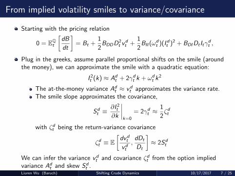
From implied volatility smiles to variance/covariance

Starting with the pricing relation

0 = EQt

[dB

dt

]= Bt +

1

2BDDD

2t v

dt +

1

2BII (ω

dt )(I dt )2 + BDIDt Itγ

dt ,

Plug in the greeks, assume parallel proportional shifts on the smile (aroundthe money), we can approximate the smile with a quadratic equation:

I 2t (k) ≈ Adt + 2γdt k + ωd

t k2

The at-the-money variance Adt ≈ vd

t approximates the variance rate.The smile slope approximates the covariance,

Sdt ≡

∂I 2t∂k

∣∣∣∣k=0

= 2γdt ≈1

2ζdt

with ζdt being the return-variance covariance

ζdt ≡ E[dvd

t

vdt

,dDt

Dt

]≈ 2Sd

t

We can infer the variance vdt and covariance ζdt from the option implied

variance Adt and skew Sd

t .Liuren Wu (Baruch) Shifting Crude Dynamics 10/17/2017 7 / 25

Project crude on SPX

dOt/Ot = ηdt

√vdt dW

dt − ηst

√v st dW

st

We can think of the above equation as a projection of crude futures returnonto the market portfolio (SPX) and treat dW s

t as the residual.

By projection, Et [dWst dW

dt ] = 0.

By classic asset pricing theory, there is no feedback effect on idiosyncraticrisk, Et [dW

st dv

st ] = 0.

From the at-the-money variance and skew on crude futures options, we have

Aot = (ηdt )2vd

t + (ηst )2v st = (ηdt )2Ad

t + (ηst )2v st .

Sot = 1

2E[dvo

t

vot, dOt

Ot

]=

(ηdt )3vd

t

vot

12E[dvd

t

vdt, dDt

Dt

]=

(ηdt )3Ad

t

Aot

Sdt .

Combining the two smiles gives us the demand loading (ηdt ) and the relativevariance contribution of the demand shocks (RC d

t ):

ηdt =

(Sot A

ot

Sdt A

dt

)1/3

, RC dt =

(ηdt )2Adt

Aot

.


Constructing floating implied variance and skew series

SPX options are listed at CBOE. Crude (WTI) futures options at CME.

Options contracts are with fixed strikes and expiry dates.

We choose three-month at the pivot point and construct the at-the-moneyimplied variance (At) and implied variance skew (St) from the optionobservations.

Convert option prices into BMS implied volatilities.

At each observed maturity, perform local quadratic regression togenerate implied volatility estimates at floating moneyness levels k

Linear interpolation on total variance to obtain estimates at 3-monthmaturity.

Shorter maturity is noisier. Longer maturity is sparse. A quarter horizon isabout right for hedging.


Time-variation of the ATM implied volatilities

04 05 06 07 08 09 10 11 12 13 14 15 16 170

10

20

30

40

50

60

70

80

90AT

M im

plie

d vo

latil

ity, %

WTI

SPX

The two series show more independent variations during the first half of thesample, but more comovements during the second half.

Cross-correlation between daily log changes: 26% before 2010, 41% after.


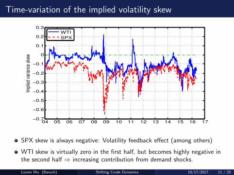
Time-variation of the implied volatility skew

04 05 06 07 08 09 10 11 12 13 14 15 16 17−0.7

−0.6

−0.5

−0.4

−0.3

−0.2

−0.1

0

0.1

0.2

0.3Im

plie

d va

rianc

e sk

ew

WTI

SPX

SPX skew is always negative: Volatility feedback effect (among others)

WTI skew is virtually zero in the first half, but becomes highly negative inthe second half ⇒ increasing contribution from demand shocks.


Shifting demand shock contribution to crude movements

04 05 06 07 08 09 10 11 12 13 14 15 16 170

10

20

30

40

50

60

70

80

90

100V

aria

nce

cont

ribut

ion

from

dem

and

shoc

ks, %

Demand shock contributes little to crude movements before 2009, but over50% since then.

What’s driving the shift and what’s the implication?


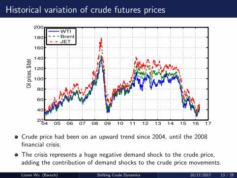
Historical variation of crude futures prices

04 05 06 07 08 09 10 11 12 13 14 15 16 1720

40

60

80

100

120

140

160

180

200O

il pr

ices

, $/b

bl

WTIBrentJET

Crude price had been on an upward trend since 2004, until the 2008financial crisis.

The crisis represents a huge negative demand shock to the crude price,adding the contribution of demand shocks to the crude price movements.


The US shale revolution

04 05 06 07 08 09 10 11 12 13 14 15 16 1710

20

30

40

50

60O

PE

C p

rodu

ctio

n, m

bb/d

04 05 06 07 08 09 10 11 12 13 14 15 16 171

2

3

4

5

6

US

tigh

t oil,

mbb

/d

Year

OPEC production has been stable over the sample period.

US tight oil production has picked up pace since 2010, from negligible to17% of OPEC production.


The history

Oil entered human history as an energy source in the mid 1800s.

The US started and dominated crude production and consumption until1970s, when the center of the market started shifting to the Gulf, wherecrude can be produced cheaply via primary and secondary oil recovery.

Primary oil recovery: crude that naturally rises to the surface, or thosethat use artificial lift devices, such as pump jacks.Secondary recovery employs water and gas injection, displacing the oiland driving it to the surface.

By forming a cartel, the OPEC countries had been able to control crudeproduction to maximize surplus.

The low production cost and the abundant reserves are what giveOPEC the market price-setting power.

Since 2010, advances in technology (horizontal drilling, hydraulic fracturing)and innovative financing have enabled US companies to produce tight oilfrom shales via enhanced oil recovery at competitive cost.

The center of energy might be shifting back to the US ...


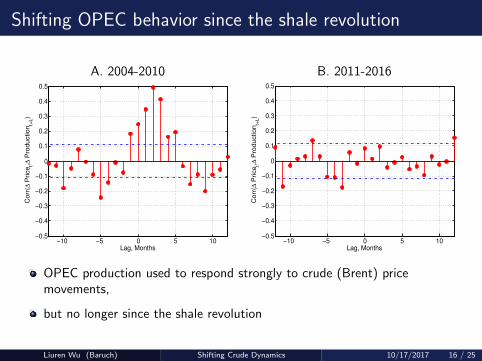
Shifting OPEC behavior since the shale revolution

A. 2004-2010 B. 2011-2016

−10 −5 0 5 10−0.5

−0.4

−0.3

−0.2

−0.1

0

0.1

0.2

0.3

0.4

0.5

Lag, Months

Corr

(∆ P

rice

t,∆ P

roduction

t+L)

−10 −5 0 5 10−0.5

−0.4

−0.3

−0.2

−0.1

0

0.1

0.2

0.3

0.4

0.5

Lag, MonthsC

orr

(∆ P

rice

t,∆ P

roduction

t+L)

OPEC production used to respond strongly to crude (Brent) pricemovements,

but no longer since the shale revolution


Shifting crude dynamics and market sentiments

The financial crisis represents a large negative demand shock that put a dentto the crude price.

The subsequent rise of the shale revolution has fundamentally altered thecrude supply behavior.

The increasing U.S. shale oil production at a competitive cost has undercutthe price-setting power of the OPEC, and lowered the OPEC’s incentive toself-regulate its production.

As a result of the shift in dynamics, investors have also shifted from beingconcerned with crude oil price hikes as a gauge of production cost, toworrying about crude oil price declines as an indication of weakening marketdemand.

Crude futures option implied volatilities turned from showing positiveor no skew to showing negative skew.


Implications for fuel cost hedging

The purpose of hedging is to reduce variation in the bottom line.

Reduce bottom-line variation can reduce financial vulnerability.

We can decompose an airline company’s bottom line into revenue and cost.

Revenue fluctuation is mainly driven by aggregate market demand,which we can assume proportional to variation in the stock index (Dt).

Cost variation is mainly driven by variation in jet fuel cost, which wecan proxy with variation in crude futures price Ot .

Schematically, we can decompose the variation of the airline company’sunhedged bottom line variation as

dUAt

UAt= βr

dDt

Dt− βc

dOt

Ot= (βr − βcηdt )

√vdt dW

dt + βcη

st

√v st dW

st

βr , βc capture the exposure to demand shock and oil shock.

When the fuel cost variation is fully hedged with crude futures, the hedgedbottom line variation becomes

dHAt

HAt= βr

dDt

Dt= βr

√vdt dW

dt


Fuel cost hedging effectiveness under different markets

Compare the bottom line variation for hedged and unhedged operations:

dUAt

UAt= (βr − βcηdt )

√vdt dW

dt + βcη

st

√v st dW

st ,

dHAt

HAt= βr

√vdt dW

dt

When crude variation is dominated by supply shocks and demand shock issmall (v s

t � vdt ∼ 0), hedging fuel cost variation effectively removes bottom

line variation, as VHA = β2r v

dt ∼ 0.

This is the original idea of fuel cost hedging, with fuel cost variationimplicitly regarded as driven by supply shocks independent of demand.

When demand shocks dominate the crude variation (vdt � v s

t ∼ 0), theunhedged bottom line can show smaller variation than the hedged bottomline, (βr − βcηdt )2 < β2

r with βr ≥ βcηdt .

When demand shock dominates, crude price increases with increaseddemand, and decline with reduced demand.Fuel cost positively co-moves with demand and hence revenue, thuscan partially cancel out the revenue variation.


Optimal dynamic fuel cost hedging

Let ht denotes the optimal fraction of hedging against fuel cost. Thepartially hedged bottom line dynamics becomes

dPAt

PAt= (βr − (1− ht)βcη

dt )

√vdt dW

dt + (1− ht)βcη

st

√v st dW

st .

We choose ht to minimize the bottom line variation

minht

(βr − βc(1− ht)η

dt

)2vdt + β2

c (1− ht)2(ηst )2v s

t

⇒ ht = 1 − βrβc

ηdt vdt

vot

The optimal hedging ratio depends crucially on the relative composition.

Full hedge when demand shock contribution is small (zero)Partial or no hedge when demand shock dominates.

We can map the hedging ratio to the option ATM implied variance and skewestimates:

ht = 1 − βrβc

(Sot

Sdt

)1/3 (Adt

Aot

)2/3

.


Shifting optimal hedging ratio for fuel cost hedging

04 05 06 07 08 09 10 11 12 13 14 15 16 170.2

0.3

0.4

0.5

0.6

0.7

0.8

0.9

1O

ptim

al fu

el c

ost h

edgi

ng ra

tio, h

t

Full fuel cost hedging is optimal historically.

only partial hedge in the current demand-driven crude market.


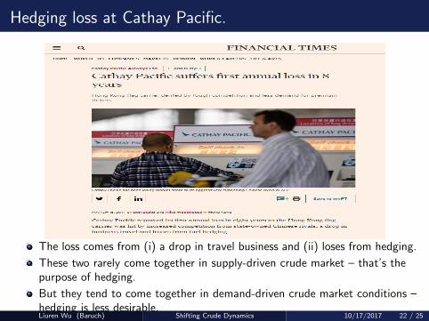
Hedging loss at Cathay Pacific.

The loss comes from (i) a drop in travel business and (ii) loses from hedging.

These two rarely come together in supply-driven crude market – that’s thepurpose of hedging.

But they tend to come together in demand-driven crude market conditions –hedging is less desirable.Liuren Wu (Baruch) Shifting Crude Dynamics 10/17/2017 22 / 25

Delta loss to crude hedging

The $4bn loss in the last 8 years is not due to “wrong bet,” but due to“wrong hedge.”

Crude movements during the last 8 years are much more driven by demandthan supply, and asking for less or no fuel cost hedging.Liuren Wu (Baruch) Shifting Crude Dynamics 10/17/2017 23 / 25

Ignore the shifting market condition at your own peril

It is difficult to predict whether the crude price will go up or down.

Delta CEO Bastian: “I don’t get paid to make those kinds of bets.”

Predicting the second moments (variance/covariance) is much easier,especially with options.

We can infer the time-variation in the relative contribution of demand shocksto the crude price movements from stock index and crude futures options,

without making directional bets,

without pretending to know whether there are different regimes andhow they transit from one to another.

The inferred relative contribution can be used to determine the optimal fuelhedging ratio, which can drastically reduce the cost/loss of the foolhardypractice of full fuel hedge.

In a demand-driven market, the full hedge fully exposes the airline todemand shocks.


Concluding remarks

Historically, oil prices have gone through many up and down cycles.

Predicting where the price goes next is immensely useful but difficult to do.

It can also be beneficial if we can predict or identify at an early stage themajor driving forces of the upcoming cycle.

Demand-driven price movements have drastically different economicand financial implications than supply-driven price movements.

We propose a semi-parametric approach to identify the time-varyingmagnitudes of demand and supply shocks from options on crude futures andthe stock index.

An analysis of the recent decades reveals a shift from supply-dominatedfluctuations to demand-dominated fluctuations.

The shift was started by the large negative demand shock shock of the 2008financial crisis, and henceforth perpetuated by the shale revolution.

Accounting for the shift alters the optimal hedging strategy for the airlineindustry and can bring potentially huge savings to their bottom line.


Date post:	07-Feb-2022
Category:	Documents
Upload:	others
View:	2 times
Download:	0 times

Shale Revolution and Shifting Crude Dynamics

Documents