Shape Optimization of Transfer Functions^

Jiawang Nie and James W. Demmel

Department of Mathematics, University of California, Berkeley, CA 94710, USA. {nj w,demmel}9math.berkeley.edu

Summary. We show how to optimize the shape of the transfer function of a linear time invariant (LTI) single-input-single-output (SISO) system. Since any transfer function is rational, this can be formulated as an optimization problem for the coefficients of polynomials. After characterizing the cone of polynomials which are nonnegative on intervals, we formulate this problem using semidefinite programming (SDP), which can be solved efficiently. This work extends prior results for discrete LTI SISO systems to continuous LTI SISO systems.

K e y words: Linear system, transfer function, shape optimization, nonnega­tive polynomials, convex cone, semidefinite programming.

1 Introduction

Consider the following linear time invariant (LTI) single-input-single-output (SISO) system

i = Ax + bu (1)

y = c^x + du (2)

where yl € K"^" , 6, c G R " , d £ R. The transfer function is H{s) = d + c^{sl-A)~'^b, which can also be written as the rational function

ELpQ'fc's' ' = gi(g)

Note tha t deg[qi) < deg(g2) < n. Conversely any function H{s) of this kind is the transfer function of some

LTI system. Any such a LTI system is called a realization of H{s). There are many such (algebraically equivalent) LTI systems [CD91, chap. 9].

* This research was supported by the National Science Foundation Grant No. EIA-0122599.

314 Jiawang Nie and James W. Demmel

In many engineering applications, we want the transfer function to have certain attractive properties. For example, we may want the Bode plot (the graph of |i?(s)| along the pure imaginary axis s = j • UJ) to have a certain shape corresponding to some kind of filtering. In this paper we study the shape optimization problem of choosing the coefficients of the rational function H{s) so its Bode plot has some desired shape.

Now consider a discrete LTI system, i.e. the governing differential equation (l)-(2) is replaced by the difference equation 52fc=i C(kz{n—k) = X]^=i Pe.v[n— t) where {u(fc)}^j is a sequence of discrete inputs and {z{k)}^^^ is the se­quence of state variables. In this case there are several nice papers [AV02, GHNOO, WBV97] that show how to formulate the filter design problem as the solution of the feasibility problem for certain convex sets. The main idea is to apply the spectral factorization of trigonometric polynomials, a characteriza­tion of nonnegative univariate polynomials, and semi-infinite programming. This approach can be used to design the transfer function to be a bandpass filter, piecewise constant or polynomial, or even have an arbitrary shape.

Our contribution is to extend these results to continuous time LTI SISO systems (l)-(2). In this case the transfer function is not a trigonometric poly­nomial and hence we cannot directly apply spectral factorization. Fortunately our transfer function is a univariate rational function, which lets us apply cer­tain characterizations of nonnegative univariate polynomials over the whole axis (—00,00), semi-axis (0,oo), or some finite interval [a,5]; see section 2. Using these characterizations, we show how to solve the shape optimization problem for the following shapes:

1. standard bandpass filter design; 2. arbitrary piecewise constant shape; 3. arbitrary piecewise polynomial shape; 4. general nonnegative function.

We will show that the first three shape optimization problems can be solved by testing the feasibility of certain convex sets, which are the intersections of certain hyperplanes and the cone of semidefinite matrices. This feasibility testing can be done efficiently using semidefinite programming (SDP) [VB96]. The fourth shape optimization problem can be solved by semi-infinite pro­gramming (SIP) [P0I97, WBV97].

We introduce some notation. For any m G N, denote by 5"* the vector space of m — by — m symmetric matrices, and let S^ be the intersection of S^ and the positive semidefinite matrices. A y B{A y B resp.) means that A — B is positive definite (semidefinite resp.). [r\ denotes the largest integer no greater than r. deg{p) is the degree of the polynomial p(-). Given a cone K C K^, y ^K 0 means that y G mtK, the interior of K. K* denotes the dual cone of K, i.e., /f* = {u e M^ : u^y > 0, Vy G K).

The rest of this paper is organized as follows. In Section 2 we give a characterization of the cone of polynomials which are nonnegative on certain intervals. In Section 3, we reformulate the shape optimization problem for

Shape Optimization of Transfer Functions 315

transfer functions to be convex optimization, and also discuss related work. In Section 4 we show how to recover the transfer function from its absolute value. Section 5 draws conclusions.

2 Cone of nonnegative polynomials on intervals

We characterize univariate polynomials which are nonnegative on certain in­tervals. For a survey paper see [PROO].

First, we characterize the nonnegative polynomials on the positive semi-axis [0, oo). The following result is due to Markov and Lukacs about one century ago.

Theorem 1 (Markov, Lukacs [Lukl8, Mar48, PS76]). Let q{t) G be a real polynomial of degree n. Let rii = [^J and n2 = L^^J • //'?(*) ^ 0 for all f > 0, then q{t) = qiit^ + 92(0^ where deg{qi) < n\ and deg{q2) < n2-

Now we apply this theorem to characterize the transfer function, which is similar to the spectral factorization for trigonometric polynomials. Observe that

l92(jt^)P \q2,even{j(^) + q2,odd{joj)\'^

921(^2)2-I-w2g22(w2)2

___ Pljw) 2 = —-,—r where w = u

P2[w)

Here qi^even and qi^odd denotes the even and odd parts of the polynomial gj, and qij,i,j = 1,2 are defined accordingly. Note that pi{w) and P2{w) are nonnegative polynomials on w £ [0, oo). Conversely, by Theorem 1, given any such nonnegative pi{w) and P2{w), it is possible to reconstruct the qij{w), and so qi{ju)) and H{jio). In other words, p\{w) and P2{w) with deg{pi) < deg{p2) satisfy \H{ju)\'^ = Pi{w)/p2{w) where w = u'^ for some transfer function H{juj) if and only if they are nonnegative on [0, oo).

The characterization of polynomials nonnegative on some finite interval [a, h] is analogous:

Theorem 2 (Markov, Lukacs [Lukl8, Mar48, PS76]). Letq{t) € R[t] be a real polynomial. Suppose q{t) > 0 for all t G [o, b], then one of the following holds.

1. If deg[q) = n = 2m is even, then q{t) = gi(t)^ + (* •" o-){b — 092(0^ where deg{qi) < m and deg{q2) < m — 1.

2. If deg{q) = n = 2TO + 1 is odd, then q{t) = {t - a)qi{t)'^ + (6 - t)q2{tf where deg{q{) < m and deg{q2) < m.

316 Jiawang Nie and James W. Demmel

In our algorithms we will need to compute the polynomials qi{jio) from Pi{w), i.e. we need computationally effective versions of Theorems 1 and 2. These are given in section 4.

To make the connection to semidefinite programming, we next characterize the polynomials nonnegative on an interval (either [0, oo) or [a,b]) by using certain convex cones. As introduced in [NesOO], define the vector of monomials v{t) = [1 t i^ • • • t""]"^ and the two convex cones of polynomials

Ko,co = {P G K"+^ : P^v{t) > 0 V i > 0}

Ka,b = {pe ]R"+i : p'^v{t) > 0 V e [a, b]}.

Let Hn,i G 5"+i be the i-th Hankel matrix, i.e., H^\=\^' if /e + / = i + 1, ' lO, otherwise.

As introduced in [NesOO], define linear operators

by the following

2rn + l 2n2 + l ^l{v) = Yl '^i^rii,i: ^2(-y) = Yl ^i+l^n2,i-

i=l i= l

Another two operators A^, and A/^ are defined according to whether n is even or odd. When n = 2m,

yl3 : ]R"+i-> S'™+\ Ai-.W+^^S"^

are defined as

2m+l 2 m - 1

M{v) = Yl '"i^rn.i, Ai{v) = ^ [(a + b)ViJ^i - Vi+2 " a K ] ^ m - l , i -i = l i = l

When n = 2m + 1,

yl3 :M»+i ^5-"^+!, yl4 : ]R"+i-^ 5""+i

are defined as

2m+l 2m + l

^3(w) = YZ [ »+l ~ "^il-^n^.i' ^4(^) = Yl, [ » ~ •' i+ll'f^m.i-i= l i= l

Let yli,yl2,yl3,^4 be their adjoint operators respectively, with respect to the inner product < A,B >= trace{A^B) for symmetric matrices of the same size. The following theorem is a compact characterization of cones ii'o.ooi -^o,b and their dual cones.

Shape Optimization of Transfer Functions 317

Theorem 3 (Nesterov [NesOO]). The cones Ko^(X), Ka^b can be chcLrcictev-ized as follows

1- -f o.oo f^fid its dual KQ ^ are characterized as follows:

i o.oo = {P G R"+i : p = AUYi) + A*^iY2), Yi e 5!f>+\F2 G Sl'^'},

^o.oo = {c G lR"+i : yli(c) h 0, A2{c) h 0};

2. when n = 2m is even,

Ka,b = {P G R"+i : p = AliYs) + yi:(F4),1^3 G 5!f'+\y4 G S!^},

Kl, = {c G ]R"+i : yl3(c) ^ 0,yl4(c) >r 0};

when n — 2m + 1 is odd,

K,,b = {P G R"+i : p = AUYs) + A^Y^), Y3 G 5!^+\y4 G 5!^+i},

i r ;^ = {c G R"+i : .13(c) h 0 , ^ ( c ) ^ 0};

3. Both Ko^aoiKa,b) and KQ^{K*I^) are convex, closed, and pointed cones with non-empty interiors.

Now suppose we have L subintervals of [0,00): {[ai,bi]}i=,i- Let K = i o.oo X Ka,,bi X • ••Ka^,bj^. Then its dual K* = K^^ x K*^f,^ x • • • K*^,,^. Given a matrix A of (L + l)(n + 1) rows and 2(n + 1) columns, consider the following problem:

find a vector ( if it exists ) p e K^Cn+i) s.t. Ap G K.

This can be done by solving a SDP feasibility problem by Theorem 3, say, using the SDP solver in [Stu99]. However it will introduce 2{L+ 1) symmetric matrices of size [n/2] or [n/2] + 1. In order to use interior-point methods to solve it, the complexity of one iteration will be at least 0(2(L + ^)n^) arithmetic operations. Fortunately, the dual cone K* ( does not involve two symmetric matrices. A natural barrier function [NN94] for K* is given by

L

F{c) = -lndetyli(co) -lndetyl2(co) - ^ ( l n d e t 4 ' ^ ( c i ) + Indetyl^'^(ci)),

where 713(714) is the operator A3{A4) corresponding to Kai,bi in Theorem 3. Here the vector c = (CQ, • • • , cz,) G IR""*"- x • • • R""'"^ Now solve the following

L+i times analytic center problem:

min F{c) (3)

s.t. A'^c = 0,ceintK*. (4)

318 Jiawang Nie and James W. Demmel

The barrier function F{c) will tend to infinity as c approaches dK*. Hence the minimum will be attained in the interior of K*, which is not empty as guaranteed by Theorem 3. The optimality condition is that

VF{c)=AX, ceintK*;

A'^c = 0.

The optimal solution c* and its Lagrange multiplier A* can be found very efficiently using Newton's method. For any c G intK*, it can be shown [NN94] that VF(c) -<K 0. Therefore a strictly feasible point p* = -A* with Ap* )~K 0 is obtained immediately. In Newton's method, we need to evaluate the first and second derivatives of F{c), which takes 0(Lnln^n + L'^n) arithmetic operations by using the displacement structure of Hankel matrices [GHNOO, KS95]. The interior-point methods that solve this analytic center problem take O ( Y ^ l n - ) steps [NN94] to achieve relative accuracy e. Therefore, the total complexity is 0(Ln^'^(ln^ n + L) In ^).

3 Shape optimization

In this section, we will show how to design the transfer function of a LTI SISO system so that it has a desired Bode plot. Four kinds of shapes will be discussed: standard bandpass filter, piecewise constant, piecewise polynomial, and general shapes.

3.1 Bandpass filter design

The goal is to design a transfer function \H{ju)\'^ = ^ 4 ^ which is close

to one on some squared frequency {w = w^) interval [u)^,u;''] and tiny in a neighborhood just outside this interval. The design rules can be formulated as

Pi{w),P2{w) > 0, y w >0

P2{w) Pijw) Piiw)

<S, VwG[wlw'2]U[w{,wl2]

where the interval [wfjtOg] is to the left of \w^,w^], and [101,102] ^ t° ^^'^ right. Here a and f3 are tiny tolerance parameters (say around .05). Let pi and p2 be the vectors of coefficients of pi{w) and P2{w) respectively. Then the constraints above can we restated as

Shape Optimization ofTransfer Functions 319

Pi,P2 e Xo.oo

pi - (1 - a)p2 e K^e^^r

Using Theorem 3, we see that the above cone constraints can be expressed as Ap £ K where

• In+i 0

0 In+l In+1 [a - l ) / „ + l

-In+l ( l + / 3 ) / „ + l

—In+1 SIn+1 _—In+l ^In+1

A = P

and K ^ KQ^OO X ^O,OO X -f' ^ iu'- x - -u '.-iu x-f^w«,^ xii'^.^^r. Given (Q;,/3, 5), solve the analytic center problem (3)-(4) and then recover the coefficients p.

As introduced in [GHNOO] for the discrete case, we can also consider the following objectives:

• minimize a + /9 for fixed S and n • minimize S for fixed a, /3, and n • minimize the degree n of pi and p2 for fixed a, /?, and 6.

These optimization problems with objectives are no longer convex, but quasi-convex. This means that we can use bisection to find the solution by solving a sequence of analytic center problems.

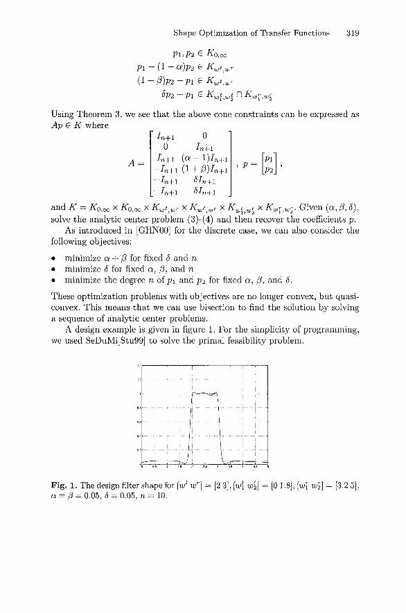
A design example is given in figure 1. For the simplicity of programming, we used SeDuMi[Stu99] to solve the primal feasibility problem.

Fig. 1. The design filter shape for [w' w''] = [2 3], [w' w'2] = [0 1.8], [wl w^] = [3.2 5], a = /3 = 0.05, 5 = 0.05, n = 10.

320 Jiawang Nie and James W. Demmel

3.2 Piecewise constant shape design

Here we extend the shape design technique from the last section to piecewise constant shapes. In other words we want the transfer function to be close to given constant values ci, ...,c„ in a set of m disjoint intervals ui"^ = w G \ak,bk], where ai < foi < a2 < 62 < • • • < Om < ^m- More precisely we want the transfer function to lie in the interval [{l—a)ck, (1 + /3)cfc] for w G [0^,6^]. By picking enough intervals (picking m large enough) we can approximate any continuous function as closely as we like.

These constraints may be written

Pii'w),P2{w) > 0, y w >0

pi{w) (1 - a)ck <

P2{w) < (1 + I3)ck, y w e [ak,bk], k = !,••• ,m.

Using Theorem 3 as before, these constraints can be rewritten as the cone constraints

Pliw),P2{w) e /tTo.oo

pi - (1 -a)ckP2, (l+/3)cfcP2 - P i e Ka^,bk,k = !,•

As before, find vector p such that Ap G K where

0

, m.

0 /n+1 (a - l)ci/„+i

( l+/?)c i /„+i - / „ + i

'n+1

(1 + f3)CmIn+l l)Cm-^n+l

and K ^ 0 , 0 0 ^ - ^ a i . b i ^ •X K? {, . Solve the analytic center problem (3)-(4) again and recover the vector p.

As in the preceding subsection, various design objectives can be considered by applying bisection. A design example for a step function with 3 steps is given in figure 2.

3.3 Piecewise polynomial shape design

Here we extend the techniques of the last section to piecewise polynomials. Thus, on each interval [afc,&fc] we ask that Pi{w)/p2{w) be close to a given polynomial (j>k{w)-, in particular that it lie in an interval [(1 — a)<j)k{w)^ (1 + (5)(j)k{w)]. This leads to the constraints

Pi{w),P2{w) > 0, V 10 > 0

{l-a)<j>k{w)<i^^<{l+l3)4>k{w), Vu;G[afc,5fc],fc = l , -- . ,m. P2\W)

Shape Optimization of Transfer Functions 321

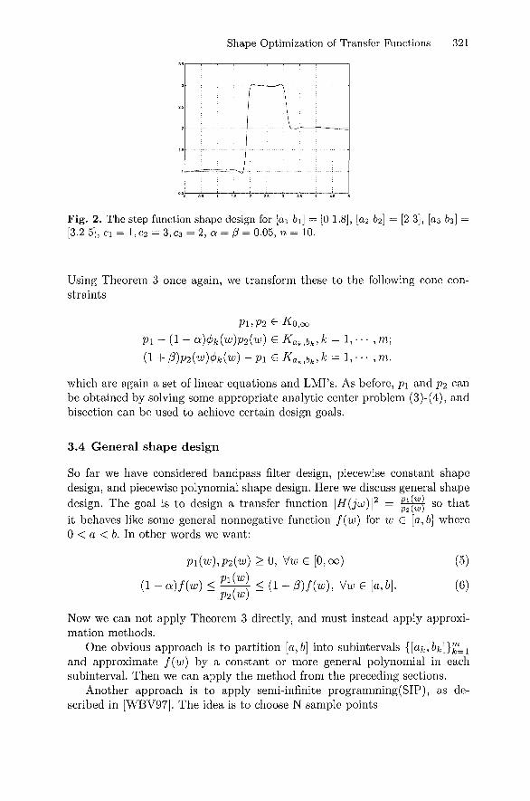
Fig. 2. The step function shape design for [ai bi] = [0 1.8], [02 62] = [2 3], [as 63] [3.2 5], ci = 1,C2 = 3,C3 = 2, a = /3 = 0.Q5, n = 10.

Using Theorem 3 once again, we transform these to the following cone con­straints

Pi - (1 - a)4>k{w)p2{'w) e Kaf,,bk,k = !,••• ,m;

(1 + (3)p2{w)(f)k{w) - p i G Ka^,bt,k = !,••• ,m.

which are again a set of linear equations and LMI's. As before, pi and P2 can be obtained by solving some appropriate analytic center problem (3)-(4), and bisection can be used to achieve certain design goals.

3.4 General shape design

So far we have considered bandpass filter design, piecewise constant shape design, and piecewise polynomial shape design. Here we discuss general shape design. The goal is to design a transfer function \H{ju>)\'^ = ^^\^l so that it behaves like some general nonnegative function f{w) for w G [a, b] where 0 < a < 6. In other words we want:

Piiw),p2{w) >0,yw& [0,00)

( l - a ) / H < Pijw) P2{w)

<{l+p)f{w), \/w€[a,b].

(5)

(6)

Now we can not apply Theorem 3 directly, and must instead apply approxi­mation methods.

One obvious approach is to partition [a,b] into subintervals {[afc,&fc]}fcLi and approximate f{w) by a constant or more general polynomial in each subinterval. Then we can apply the method from the preceding sections.

Another approach is to apply semi-infinite programming(SIP), as de­scribed in [WBV97]. The idea is to choose N sample points

322 Jiawang Nie and James W. Demmel

a < Wi < W2 < • • • < wj^ < b

and replace the semi-infinite inequality constraints (5)-(6) by N simple in­equality constraints. A standard rule of thumb is to choose A'' = 15n in prac­tice [WBV97]. Then the approximate optimization problem is solved itera-tively [Pol97].

3.5 Related work

There are several related papers [AV02, GHNOO, WBV97] on various filter design techniques. Most of them are for discrete systems, and some techniques can be applied to continuous systems with some modifications. Note that the mapping s = j ^ maps the pure imaginary axis onto the unit circle except (—1,0). Then our transfer function H{s) becomes a rational trigonometric function R{z). Each interval j[ai,bi] is mapped onto some arc {e^^ : u G [w/, wf ]} on the unit circle. The methods described in [AV02, GHNOO, WBV97] all can be applied. However, all of them will involve the constraints of the form that some trigonometric polynomial is nonnegative on some interval. The characterization of (trigonometric) polynomials nonnegative on some intervals will eventually need Theorem 3 or its equivalent form to transform to a LMI. In this paper, we transform our design problems using constraints of real polynomial nonnegativity on some intervals in the positive semi-axis. Then we may apply Theorem 3 directly to characterize these constraints using LMIs. As described at the end of Section 2, we solve an appropriate analytic center problem, instead of solving these LMIs directly. The structure of this problem can be exploited to use Newton's method to efficiently find the analytic center.

There are also several good papers [Fab02, NesOO, GHY03] on polynomials on the real axis, unit circle, pure imaginary axis, and other curves. [NesOO] is the classical paper that characterizes polynomial nonnegativity constraints by LMIs; our paper is based mostly on it. In [GHY03] the authors characterized the cone of positive pseudopolynomial matrices and discussed optimization over this cone. The authors also discussed the conditioning of such optimiza­tions, and proposed using the basis of Chebyshev polynomials to improve conditioning. [Fab02] gives an abstract version of [NesOO, GHY03], charac­terizing polynomials which are nonnegative on the disjoint union of several intervals.

4 Recovery of the transfer function

In this section, we show how to use Theorems 1 and 2 effectively. First, given polynomials pi{w) and P2{w) {w = u"^) such that ^

desired shape, we need to find real polynomials qi and q2 so that

2 Pijw)

P2{w) 92 (jw)

Shape Optimization of Transfer Functions 323

To this end, given a polynomial p{w) that is nonnegative on [0, oo), we will provide an algorithm to find two polynomials qe{w) and qo{w) such that p{w) = q1{w) + w • Qoiw). Then qe contains the even coefficients and qo the odd coefficients (modulo signs) of the desired polynomial q as described in Section 2.

Lemma 1. The following polynomial identities hold:

1. iff + wgJXfl + wgl) = {hh + wgxg2? +w{hg2 - /25i)^' 2. {w - r)2 + b^^{w- v 9 2 T F ) 2 + w • 2{Vr^+lP - r).

Proof. Verify directly. D

Lemma 2. If a polynomial p{'w) is nonnegative on [0, oo), then its factoriza­tion must have the form

( 111 \ n 2 " 3

nC-^ + Ci) Y[{.{w-rif + b^)l[{w + ai) i=l J i= l i=l

where a >0, bi > 0, n\ + 2n2 + na = n, 0 < ai < • • • < a„3, Ci < 0. Proof. Write the factorization p(tf) = a YYk=i{'^~'Pk)• First consider the constant

term a; it must clearly satisfy a > 0 for piw) to be nonnegative over [0, oo). Next consider the three classes of roots pk- real positive, complex, and real nonpositive. The positive roots must all have even multiplicity for p{w) to be nonnegative, so we can write the product of all their factors w—pk as 0^=1 (^"1" Cj) where Cj < 0. Next, the complex roots come in complex conjugate pairs Pk = Tk + j • bk and p^ = rk - j • bk, so we can write {w - Pk)iw - pk) = {w — rkY + b\ for all n2 complex conjugate pairs. Finally consider the na nonpositive real roots 0 > —ai > • • • > ~a„3 of p{w). Their corresponding factors u; — (—Oj) = u; + ttj are all nonnegative on [0, oo).

D Using the above two lemmas, we get the following algorithm.

Algorithm 4.1 This algorithm will find qe{w) and qo{w) such that p{w) = q1{w) + « ; • q1{w) if p{w) is nonnegative on [0, oo). Let ge = l>9o = 0.

Step 1 Find the factorization of

where hi > 0, ni + 2n2 + ns = n, 0 < ai < • • • < a„3,0 > Cj £ K. Step 2 Find the {-f + w{-f form ofXXZ^iw + a^)

for fc = 1 : n3 qe = y/alqe + W • qo

qo = \fa'iqo - qe qe •=qe,qo -^^qo-

end

324 Jiawang Nie and James W. Demmel

Step 3 Find the {-f + w{-f form ofY^^l^{w'^ + 6f) for k = 1 : n2

qe = qejw - ^rf + b'i) + w • g „ ^ 2 ( ^ K ' + 6f - r^)

9o = qeyj2{^rt^+yf^)- qo{w - ^rf + b'j)

Qe ••=qe,qo ••^'qo-end

Step 4 qe := aqe ]Xi=ii'^ + ^i), 9o := aQo n " = i ( ^ + ^i).

Now apply algorithm 4.1 topi{w){i = 1,2) respectively, i.e., Und qij{w){i,j = 1, 2) such that Pi{w) = qfiiw) + w • ql2{'^) fo^ i = 1, 2. Then we obtain the desired transfer function

H{s) 92,l(- 'S^) + S92 ,2 ( -S^) '

Remark: If a polynomial p{w) is nonnegative on a finite interval [—1,1] (an­other finite interval can be changed to this one by a linear transformation), then we can also apply the above algorithm to find two polynomials pi and P2 such that p{w) = Pi{w) + (1 — w){w + l)p'2{w). ActuaUy, we only need to do the Goursat transform (see [PROO]) for piw), i.e.,

p(«;) = (^ + l ) " p ( i ^ ) ,

and then apply the above algorithm to find qe,qo such that

p{w) =ql{w)+wqliw),

and then apply the inverse Goursat transform to get back p{w):

p{w) = 2-"(w + l)'*''ff(P)p(i-^^).

5 Conclusions and discussion

This paper discusses shape optimization for a transfer function for a LTI SISO system by formulating it via semidefinite programming. Given the shape (absolute value) of the transfer function, we show how to extract the transfer function itself. Since the optimization process uses semidefinite programming, it may be done efficiently.

We do not consider any constraints on the components A, b, c, d of the LTI system. However in practice, these components may not be arbitrary, but instead have special structure and depend on certain design parameters. Thus an interesting question is finding those parameters to optimize the shape of the transfer function as we did in Section 3. This is in general not a convex

Shape Optimization of Transfer Functions 325

problem, and can be very hard to solve. But it is still a feasibility/optimization problem about polynomials, if {A, b, c, d) are polynomials in those parameters. Therefore, we may formulate them using polynomial optimization, and then solve them by techniques such as the sum of squares and positivstellensatz (see [ParOl]). But this is more difficult, and future work.

A c k n o w l e d g e m e n t s : The authors would like to thank Prof. El Ghaoui and the Referee for many useful comments and suggestions.

References

[AV02] B. Alkire and L. Vandenberghe, Convex optimization problems involving finite autocorrelation sequences. Mathematical Programming Series A 93 (2002), 331-359.

[CD91] Prank M. Callier, Charles A. Desoer, Linear System Theory, Springer-Verlag, New York, 1991.

[Fab02] L. Faybusovich, On Nesterov's approach to semi-infinite programming. Acta Applicandae Mathematicae 74 (2002), 195-215.

[GHNOO] Y. Genin, Y. Hachez, Yu. Nesterov, P. Van Dooren, " Convex Optimization over Positive Polynomials and filter design", Proceedings UK A CC Int. Conf. Control 2000, page SS41, 2000.

[GHY03] Y. Genin, Y. Hachez, Yu. Nesterov, P. Van Dooren, Optimization problems over positive pseudopolynomial matrices, SIAM Journal on Matrix Analysis and Applications 25 (2003), 57-79.

[KS95] T. Kailath and A.H. Sayed, "Displacement Structure: theory and applica­tions", SIAM Rev. 37(1995), 297-386.

[LuklS] Lukacs, "Verscharfung der ersten Mittelwersatzes der Integralrechnung fur rationale Polynome", Math. Zeitschrift, 2, 229-305, 1918.

[Mar48] A.A. Markov, "Lecture notes on functions with the least deviation from zero", 1906. Reprinted in Markov A.A. Selected Papers (ed. N. Achiezer), GosTechlzdat, 244-291, 1948, Moscow(in Russian).

[NN94] Yu. Nesterov and A. Nemirovsky, "interior-point polynomial algorithms in convex programming", SIAM Studies in Applied Mathematics, vol. 13, Soci­ety of Industrial and Applied Mathematics(SIAM), Philadelphia, PA, 1994.

[NesOO] Yu. Nesterov, "Squared functional systems and optimization problems". High Performance Optimization(H.Frenk et al., eds), Kluwer Academic Publishers, 2000, pp.405-440.

[Pol97] E. Polak, "Optimization: Algorithms and Consistent Approximations". Ap­plied Mathematical Sciences, Vol. 124, Springer, New York, 1997.

[PS76] G. Polya and G. Szego, Problems and Theorems in Analysis II, Springer-Verlag, New York, 1976

[PROO] V. Powers and B. Reznick, "Polynomials That are Positive on an Interval", Transactions of the American Mathematical Society, vol. 352, No. 10, pp. 4677-4692, 2000.

[WBV97] S.-P. Wu, S. Boyd, and L. Vandenberghe, "FIR filter design via spectral factorization and convex optimization". Applied and Computational Con­trol, Signals and Circuits, B. Datta, ed., Birkhauser, 1997, ch.2, pp.51-81.

326 Jiawang Nie and James W. Demmel

[ParOl] P.A. Parrilo. Semidefinite Programming relaxations for semialgebraic prob­lems. Math. Prog., No. 2, Ser. B, 293-320, 96 (2003).

[Stu99] J.F. Sturm, "SeDuMi 1.02, a MATLAB toolbox for optimization over sym­metric cones". Optimization Methods and Software, ll&£:12(1999)625-653.

[VB96] L. Vandenberghe and S. Boyd, "Semidefinite Programming", SIAM Review, 38(l):49-95, 1996.