SHAPE Ver. 1.3 A Software Package for

Quantitative Evaluation of Biological Shapes

Based on elliptic Fourier descriptors

Developed by

Hiroyoshi Iwata

Last update: 2006.12.26

1

SHAPE ver. 1. 3 Copyright © 2001, 2006 National Agricultural Research Organization. All rights reserved.

This program is freely distributed in the hope that it will be useful, but WITHOUT ANY WARRANTY; without even the implied warranty of MERCHANTABILITY or FITNESS FOR A PARTICULAR PURPOSE.

Contact Information: Hiroyoshi Iwata (Ph. D) Data­mining and Grid Research Team National Agricultural Research Center National Agricultural Research Organization 3­1­1 Kannondai, Tsukuba, Ibaraki 305­8666, Japan Tel: +81­298­38­7025, Fax: +81­298­38­8551 e­mail: iwatah@affrc.go.jp Web page: http://cse.naro.affrc.go.jp/iwatah

2

Table of Contents

0. Caution

1. Introduction

2. System Requirements

3. Installation

4. Preparation of Image files

5. Image analysis program ­ ChainCoder

6. Elliptic Fourier transformation program ­ Chc2Nef

7. Principal component analysis program ­ PrinComp

8. Contour visualization program – PrinPrint

9. ViwerPrograms – ChcViewer and NefViewer

10. About sample files

11. How to cite SHAPE

12. Acknowledgements

13. References

14. Appendix

Elliptic Fourier Descriptors

3

0. Caution

! Caution If you have been a user of the older version of SHAPE, please beware of the following point:

I found a bug in SHAPE ver.1.2, which has been fixed in SHAPE ver.1.3. Because of this bug, chain­code obtained by SHAPE ver.1.2 traces an object's contour “clockwise”, although it is expected to trace a contour “counter­clockwise” in general (you can check the direction of contour trace by the viewer programs, ChcViewer and NefViewer). EFDs derived from clockwise chain­code are different from ones derived from counter­clockwise code in the sign of coefficients b and d. As indicated in Table 1, the difference in the sign of the coefficients may not cause any serious problem in the shape analyses, if all EFD or chain­code data are obtained by the same version of SHAPE. However, it should cause a serious artifact, if you analyze jointly the data obtained by the different version of SHAPE. Please be sure NEVER TO ANALYZE JOINTLY EFD or chain­code data obtained by THE DIFFERENT VERSION OF SHAPE! For the joint analysis, please use converter programs to convert the direction of contour trace of chain­code or EFDs obtained by SHAPE ver.1.2.

I greatly apologize for the inconvenience.

Table 1. Direction of contour trace and problems in shape analyses EFD and

chain­code Data Direction of contour trace Problems in shape analyses Ways of coping

Data obtained by SHAPE ver.1.2 Clockwise No problem Not necessary

Data obtained by SHAPE ver.1.3 Counter­clockwise Of course, No problem Not necessary

Combined data obtained by both versions

The mixture of clockwise and contour­clockwise

The difference in the direction of contour trace causes the difference in the sign of Fourier coefficients b and d. This should cause a serious artifact in the analyses

Use converter programs before analyzing the conbined data

4

Introduction

Methods for the quantitative evaluation of biological shapes are valuable for researchers in various fields, such as genetics, agriculture, ecology and taxonomy. Elliptic Fourier descriptors (EFDs), originally proposed by Kuhl and Giardina (1982), can delineate any type of shape with a closed two­dimensional contour. EFDs have been effectively applied to the analysis of various biological shapes in animals (Rohlf and Archie 1984; Ferson et al. 1985; Bierbaum and Ferson 1986; Diaz et al. 1989; Liu et al. 1996; Laurie et al. 1997) and plants (White et al. 1988; McLellan 1993; Furuta et al. 1995; Ohsawa et al. 1998; Iwata et al. 1998; Iwata et al. 2000; Toyohara et al. 2000; Iwata et al. 2002; Uga et al. 2003: Iwata et al. 2004a, 2004b; Yoshioka et al. 2005a, 2005b, 2006a, 2006b). Evaluation based on EFDs also gives sufficient resolution¸ in combination with quantitative genetic analysis, to elucidate the inheritance of biological shapes.

However, although EFDs can be powerful tools for the analysis of biological shapes they are not easy to apply, since several complex procedures are involved, such as image­processing, contour­recording, derivation of the descriptors and multivariate analysis of the descriptors.

For this reason, I developed SHAPE, a software package for evaluating contour shapes based on EFDs. SHAPE contains four programs named ChainCoder, Chc2Nef, PrinComp and PrinPrint for processing digital images, obtaining EFDs, performing principal component analysis and visualizing shape variations explained by the principal components, respectively. With the aid of this package, a researcher can easily analyze shapes on a personal computer without special knowledge about the procedures involved in the method.

I hope that SHAPE will be used by many researchers in diverse fields and that it will help elucidate various important aspects of biological shapes in the future.

5

1. System Requirements

The programs contained in SHAPE can be executed on any IBM compatible computer running Windows 95, 98, NT or higher versions.

2. Installation

1. Download the zipped file named "shape.zip", which contains all the SHAPE files. The file is available at the website ”http://cse.naro.affrc.go.jp/iwatah/shape”. The files contained in "shape.zip"* are as follows:

ChainCoder.exe an execute file for the program ChainCoder CHC2NEF.exe an execute file for the program Chc2Nef PrinComp.exe an execute file for the program PrinComp PrinPrint.exe an execute file for the program PrinPrint ChcView.exe an execute file for the program ChcView NefView.exe an execute file for the program NefView bmp_work.dll a dynamic link library used by ChainCoder imgprc.dll a dynamic link library used by ChainCoder Princomp.dll a dynamic link library used by PrinComp Prinscore.dll a dynamic link library used by PrinComp Prinplot.dll a dynamic link library used by PrinPrint Sample_img.bmp a sample image file Sample_chc.chc a sample of chaincode file Sample_nef.nef a sample of normalized EFDs file Tutorial.pdf a tutorial for understanding how to use SHAPE Manual.pdf this file (a manual for SHAPE)

* “shape_s.zip” does not contained the sample, tutorial and manual files.

2. Create a new folder named "shape".

3. Extract all the files from "Shape.zip" to the "shape" folder.

4. You can run any program by double­clicking its icon in the “shape” folder.

6

Preparation of image files

SHAPE can only handle FULL COLOR (24­bit) BITMAP (*.bmp) images, and CANNOT HANDLE 256 COLOR, 16 COLOR, or MONOCHROME bitmap images. So, if you have files of images in a different format, such as jpeg or 256­color bitmap, you have to convert them to full color (24­bit) bitmap format prior to analysis. “Microsoft Paint” that comes with Microsoft Windows can convert the file formats. Graphic programs such as "Paint Shop Pro" may be more suitable for this purpose. "Paint Shop Pro" can convert the file format of all the images within a folder in a single operation.

When you prepare images of objects, please pay attention to the following points: 1. If you want to measure the size of the objects: i.e. their area and perimeter, a scale marker should be included with each image. The marker should be a square or rectangle of defined size (e.g. 30 mm x 30 mm) placed above, below, or to the left or right of the image (see the file "Sample_img.bmp" accompanying SHAPE for an example).

2. When you take images, you do not need to pay strict attention to the orientation of the objects. Although it is better to align them, at least roughly, their orientation is standardized mathematically in the derivation of the normalized EFDs.

3. SHAPE can process multiple objects in a single image. In other words, you can place more than one object for analysis in each image. In such cases, please take care that none of the objects overlap each other.

4. If the objects have a comparatively bright color, it is better to use a black background. However, if the objects are dark, the background should be bright (white).

5. If the objects are not flat, it is recommended to light them from behind when taking their image, to suppress differences in shading on their surfaces (see the "Sample_img.bmp").

6. If objects have a flat, essentially two­dimensional shape (for instance, plant leaves), an image scanner can be used to take their images. In general, however, a digital camera will be best suited for this purpose.

7

4. Image analysis program ­ ChainCoder

ChainCoder extracts the contour of objects from an image file and records them as chain­code (Freeman 1974). Chain­code is a coding system for describing geometrical information about contours in numbers from 0 to 7. ChainCoder converts a full color image to a binary (black and white color) image, reduces noise, traces the contours of objects and describes the contour information as chain­code. ChainCoder outputs a chain­code file, which is analyzed by the program Chc2Nef.

Input file : A windows full color bitmap (*.bmp) file

Output file : A chain­code (*.chc) file

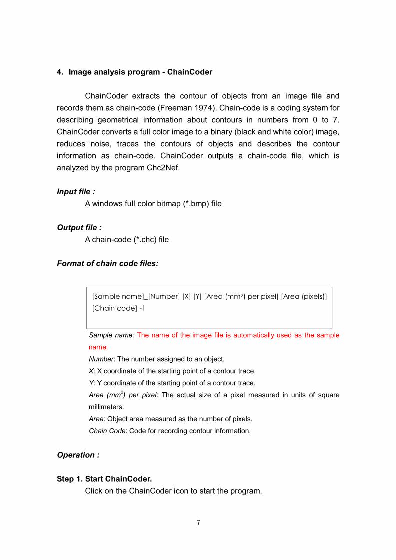
Format of chain code files:

Sample name: The name of the image file is automatically used as the sample

name.

Number: The number assigned to an object.

X: X coordinate of the starting point of a contour trace.

Y: Y coordinate of the starting point of a contour trace.

Area (mm 2 ) per pixel: The actual size of a pixel measured in units of square

millimeters.

Area: Object area measured as the number of pixels.

Chain Code: Code for recording contour information.

Operation :

Step 1. Start ChainCoder. Click on the ChainCoder icon to start the program.

[Sample name]_[Number] [X] [Y] [Area (mm 2 ) per pixel] [Area (pixels)] [Chain code] ­1

8

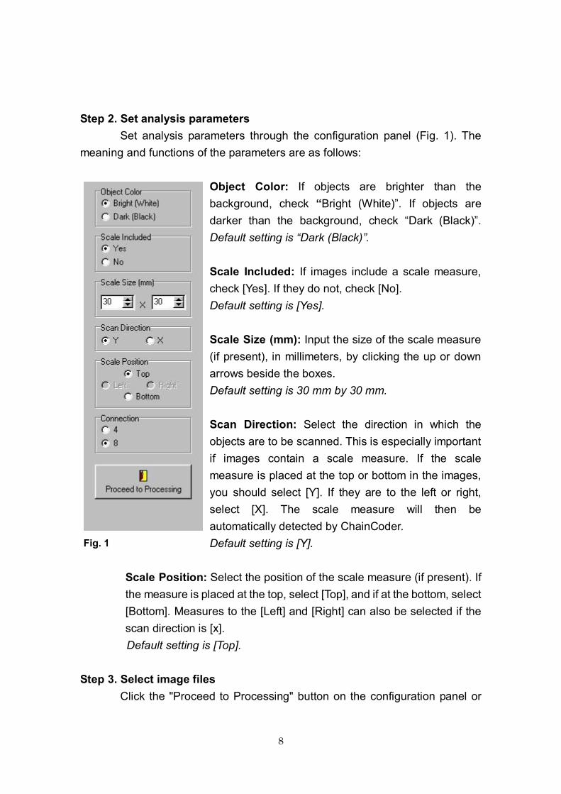
Step 2. Set analysis parameters Set analysis parameters through the configuration panel (Fig. 1). The

meaning and functions of the parameters are as follows:

Object Color: If objects are brighter than the background, check “Bright (White)”. If objects are darker than the background, check “Dark (Black)”. Default setting is “Dark (Black)”.

Scale Included: If images include a scale measure, check [Yes]. If they do not, check [No]. Default setting is [Yes].

Scale Size (mm): Input the size of the scale measure (if present), in millimeters, by clicking the up or down arrows beside the boxes. Default setting is 30 mm by 30 mm.

Scan Direction: Select the direction in which the objects are to be scanned. This is especially important if images contain a scale measure. If the scale measure is placed at the top or bottom in the images, you should select [Y]. If they are to the left or right, select [X]. The scale measure will then be automatically detected by ChainCoder. Default setting is [Y].

Scale Position: Select the position of the scale measure (if present). If the measure is placed at the top, select [Top], and if at the bottom, select [Bottom]. Measures to the [Left] and [Right] can also be selected if the scan direction is [x]. Default setting is [Top].

Step 3. Select image files Click the "Proceed to Processing" button on the configuration panel or

Fig. 1

9

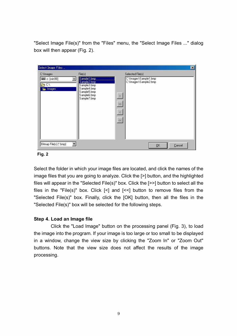
"Select Image File(s)" from the "Files" menu, the "Select Image Files ..." dialog box will then appear (Fig. 2).

Select the folder in which your image files are located, and click the names of the image files that you are going to analyze. Click the [>] button, and the highlighted files will appear in the "Selected File(s)" box. Click the [>>] button to select all the files in the "File(s)" box. Click [<] and [<<] button to remove files from the "Selected File(s)" box. Finally, click the [OK] button, then all the files in the "Selected File(s)" box will be selected for the following steps.

Step 4. Load an Image file Click the "Load Image" button on the processing panel (Fig. 3), to load

the image into the program. If your image is too large or too small to be displayed in a window, change the view size by clicking the "Zoom In" or "Zoom Out" buttons. Note that the view size does not affect the results of the image processing.

Fig. 2

10

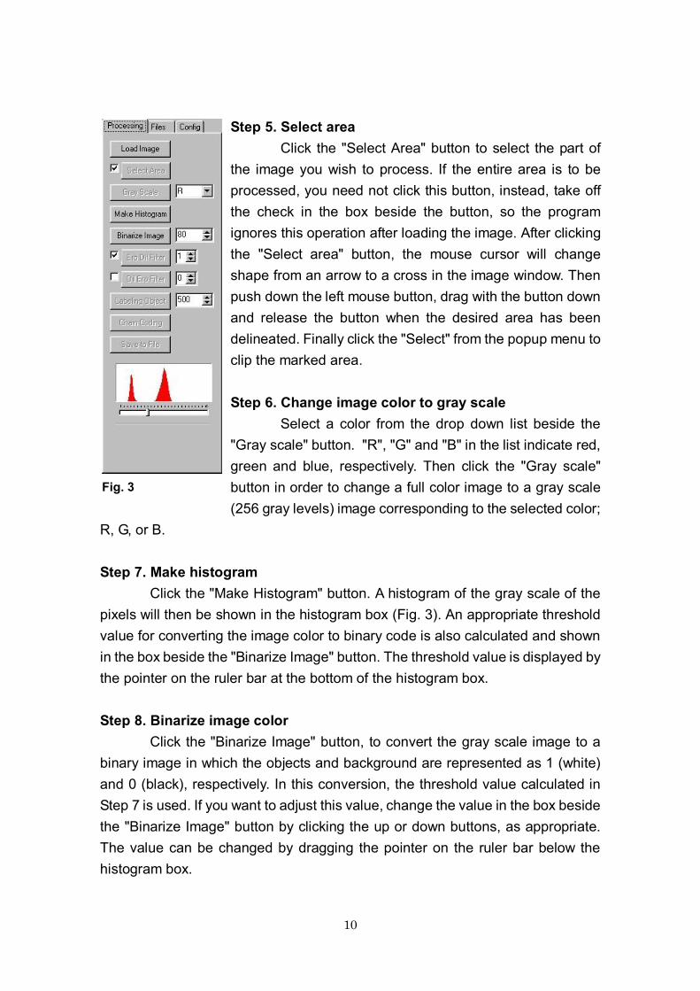
Step 5. Select area Click the "Select Area" button to select the part of

the image you wish to process. If the entire area is to be processed, you need not click this button, instead, take off the check in the box beside the button, so the program ignores this operation after loading the image. After clicking the "Select area" button, the mouse cursor will change shape from an arrow to a cross in the image window. Then push down the left mouse button, drag with the button down and release the button when the desired area has been delineated. Finally click the "Select" from the popup menu to clip the marked area.

Step 6. Change image color to gray scale Select a color from the drop down list beside the

"Gray scale" button. "R", "G" and "B" in the list indicate red, green and blue, respectively. Then click the "Gray scale" button in order to change a full color image to a gray scale (256 gray levels) image corresponding to the selected color;

R, G, or B.

Step 7. Make histogram Click the "Make Histogram" button. A histogram of the gray scale of the

pixels will then be shown in the histogram box (Fig. 3). An appropriate threshold value for converting the image color to binary code is also calculated and shown in the box beside the "Binarize Image" button. The threshold value is displayed by the pointer on the ruler bar at the bottom of the histogram box.

Step 8. Binarize image color Click the "Binarize Image" button, to convert the gray scale image to a

binary image in which the objects and background are represented as 1 (white) and 0 (black), respectively. In this conversion, the threshold value calculated in Step 7 is used. If you want to adjust this value, change the value in the box beside the "Binarize Image" button by clicking the up or down buttons, as appropriate. The value can be changed by dragging the pointer on the ruler bar below the histogram box.

Fig. 3

11

Step 9. Reduce noise with the erosion and dilation filters If noise needs to be reduced in your images, use an erosion­dilation or a

dilation­erosion filter. If the noise consists of marks like hairlines or grains of sand, the erosion­dilation filter will be most suitable. The value in the box beside the "ero dil filter" button sets the number of iterations of the erosion­dilation operation. If the value is large, large amounts of noise can be removed from your images. The "dil ero filter" is best for filling cavities in the contour (for example, if worm­eaten leaves are being analyzed).

Note that, as the time of these operations is increased, the contour of the objects becomes increasingly distorted from the original contour. Therefore, the number of iterations of the operation should be kept as low as possible.

Step 10. Label the objects Click the "Labeling Object" button. Each object will then be numbered.

The value in the box beside this button indicates the minimum pixel number covered by the objects. Objects that have an area less than this value will be ignored in the following steps. Set this value as appropriate, to insure that objects you do not wish to measure (for example, objects such as letters describing the data attribution) will not be processed.

Step 11. Get a chain code Click the "Chain Coding" button, to obtain the chain­code for each object.

Step 12. Save the chain code Click the "Save to File" button, the chain code data will then be saved in

an output file. The first time the button is used after executing this program, the "Save Chc File dialog" window will appear. Input the name of the output file and save the data. If you select the name of a file that already exists, the chain­code data is appended to the end of the file. Note that if you don't click this button, the chain­code data will not be saved anywhere. If you do not obtain a good result from Steps 4­11, you can retry the processing from Step 4 without clicking the "Save to File" button.

Step 13. Processing the next image Repeat Steps 4­12 until all the remaining images have been processed.

12

The progress of your task can be checked by clicking the "files" tab.

13

5. Elliptic Fourier transformation program ­ Chc2Nef

Chc2Nef calculates the normalized EFDs from the chain code information. The normalized EFDs are calculated in accordance with the procedures suggested by Kuhl and Giardina (1982). Chc2Nef can perform two types of normalization. One is based on the first harmonic ellipse that corresponds to the first Fourier approximation to the contour information. The size and orientation of the contour is standardized in accordance with the size and alignment of the major axis of the ellipse. The starting point for tracing the contour is also standardized with respect to the major axis. Another normalization is based on the point of the contour farthest from the center (i.e. the longest radius). This normalization is performed in accordance with the direction and absolute size of the vector from the center to the farthest point. In Chc2Nef, the normalization can be also performed manually, if desired.

Input file : A chain code (*.chc) file

Output file : A normalized EFD (*.nef) file

Format of Normalized EFD files:

Sample name, Number: Identical to those of the chain code file.

Coefficients a1­an, b1­bn, c1­cn, d1­dn: Normalized elliptic Fourier coefficients. The

value "n" corresponds to the maximum harmonic number.

Operation :

[Sample name]_[Number] [Coefficient a1] [Coefficient b1] [Coefficient c1] [Coefficient d1] [Coefficient a2] [Coefficient b2] [Coefficient c2] [Coefficient d2]

: [Coefficient an] [Coefficient bn] [Coefficient cn] [Coefficient dn]

14

Step 1. Start Chc2Nef Click the Chc2Nef icon to start the program.

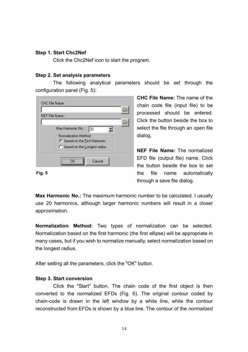
Step 2. Set analysis parameters The following analytical parameters should be set through the

configuration panel (Fig. 5): CHC File Name: The name of the chain code file (input file) to be processed should be entered. Click the button beside the box to select the file through an open file dialog.

NEF File Name: The normalized EFD file (output file) name. Click the button beside the box to set the file name automatically through a save file dialog.

Max Harmonic No.: The maximum harmonic number to be calculated. I usually use 20 harmonics, although larger harmonic numbers will result in a closer approximation.

Normalization Method: Two types of normalization can be selected. Normalization based on the first harmonic (the first ellipse) will be appropriate in many cases, but if you wish to normalize manually, select normalization based on the longest radius.

After setting all the parameters, click the "OK" button.

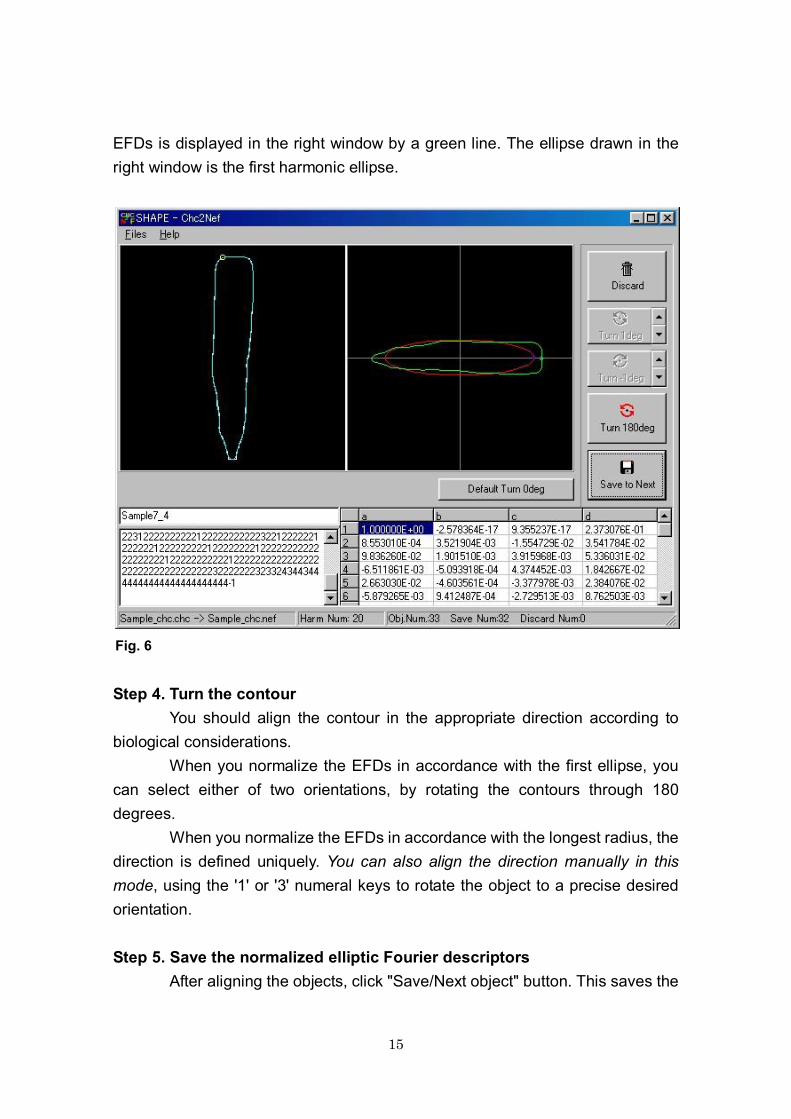
Step 3. Start conversion Click the "Start" button. The chain code of the first object is then

converted to the normalized EFDs (Fig. 6). The original contour coded by chain­code is drawn in the left window by a white line, while the contour reconstructed from EFDs is shown by a blue line. The contour of the normalized

Fig. 5

15

EFDs is displayed in the right window by a green line. The ellipse drawn in the right window is the first harmonic ellipse.

Step 4. Turn the contour You should align the contour in the appropriate direction according to

biological considerations. When you normalize the EFDs in accordance with the first ellipse, you

can select either of two orientations, by rotating the contours through 180 degrees.

When you normalize the EFDs in accordance with the longest radius, the direction is defined uniquely. You can also align the direction manually in this mode, using the '1' or '3' numeral keys to rotate the object to a precise desired orientation.

Step 5. Save the normalized elliptic Fourier descriptors After aligning the objects, click "Save/Next object" button. This saves the

Fig. 6

16

normalized EFDs to the output file named in advance. If you don't want to save the object, click the "Discard" button.

Step 6. Convert the next object After clicking the "Save/Next object" button, the next object is converted

to normalized elliptic Fourier descriptors. To convert the remaining objects, repeat steps 4 and 5 until all the objects have been converted.

17

6. Principal component analysis program ­ PrinComp

PrinComp performs a principal component analysis of the normalized EFDs derived by Chc2Nef. When a contour shape is described in the first 20 harmonics of Fourier coefficients, the number of normalized EFD coefficients becomes large (77 or 80). However, principal component analysis can efficiently summarize the information contained in these coefficients (Rohlf and Archie 1984). The principal component analysis conducted by PrinComp is based on the variance­covariance matrix of the coefficients and not on the correlation matrix, because coefficients with small variance and covariance values are generally not important for explaining the observed morphological variations. The principal component scores can be used as observed values of morphological features in subsequent analysis, such as genetic analysis of the shapes of biological organs. PrinComp outputs a principal component scores file (*.pcs) in text format with tab­stops. The scores file can be opened as an MS­Excel worksheet, and analyzed from the appropriate (e.g. biological) perspective.

Input file : a normalized EFD (*.nef) file

Output files : a principal component report (*.txt) file a principal component analysis result (*.pcr) file a principal component contours (*.pcc) file a principal component scores (*.pcs) file

Format of principal component scores files:

Sample name, Number: Identical to those in the chain­code and normalized EFD

files.

PC 1 ­ n scores: The scores of principal components. The number of principal

components, "n", can be chosen.

Operation :

[Sample Name]_[Number] [PC 1 score] [PC 2 score] ... [PC n score]

18

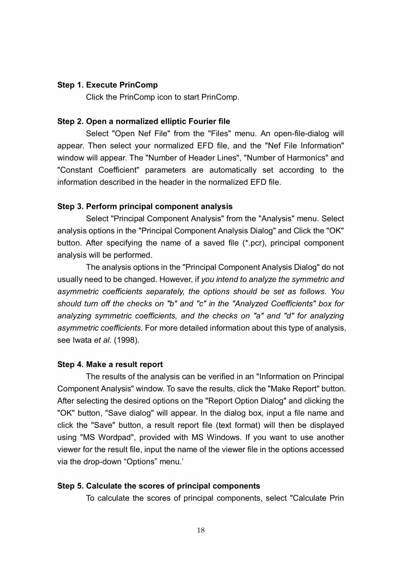
Step 1. Execute PrinComp Click the PrinComp icon to start PrinComp.

Step 2. Open a normalized elliptic Fourier file Select "Open Nef File" from the "Files" menu. An open­file­dialog will

appear. Then select your normalized EFD file, and the "Nef File Information" window will appear. The "Number of Header Lines", "Number of Harmonics" and "Constant Coefficient" parameters are automatically set according to the information described in the header in the normalized EFD file.

Step 3. Perform principal component analysis Select "Principal Component Analysis" from the "Analysis" menu. Select

analysis options in the "Principal Component Analysis Dialog" and Click the "OK" button. After specifying the name of a saved file (*.pcr), principal component analysis will be performed.

The analysis options in the "Principal Component Analysis Dialog" do not usually need to be changed. However, if you intend to analyze the symmetric and asymmetric coefficients separately, the options should be set as follows. You should turn off the checks on "b" and "c" in the "Analyzed Coefficients" box for analyzing symmetric coefficients, and the checks on "a" and "d" for analyzing asymmetric coefficients. For more detailed information about this type of analysis, see Iwata et al. (1998).

Step 4. Make a result report The results of the analysis can be verified in an "Information on Principal

Component Analysis" window. To save the results, click the "Make Report" button. After selecting the desired options on the "Report Option Dialog" and clicking the "OK" button, "Save dialog" will appear. In the dialog box, input a file name and click the "Save" button, a result report file (text format) will then be displayed using "MS Wordpad", provided with MS Windows. If you want to use another viewer for the result file, input the name of the viewer file in the options accessed via the drop­down “Options” menu.’

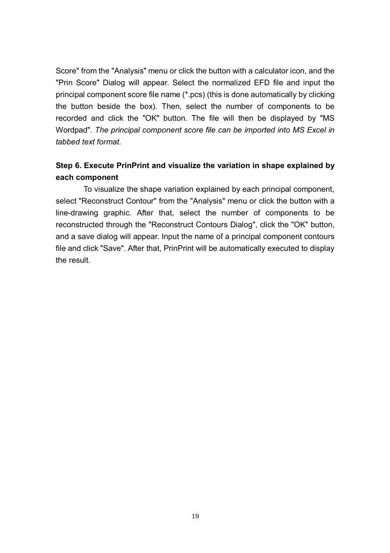
Step 5. Calculate the scores of principal components To calculate the scores of principal components, select "Calculate Prin

19

Score" from the "Analysis" menu or click the button with a calculator icon, and the "Prin Score" Dialog will appear. Select the normalized EFD file and input the principal component score file name (*.pcs) (this is done automatically by clicking the button beside the box). Then, select the number of components to be recorded and click the "OK" button. The file will then be displayed by "MS Wordpad". The principal component score file can be imported into MS Excel in tabbed text format.

Step 6. Execute PrinPrint and visualize the variation in shape explained by each component

To visualize the shape variation explained by each principal component, select "Reconstruct Contour" from the "Analysis" menu or click the button with a line­drawing graphic. After that, select the number of components to be reconstructed through the "Reconstruct Contours Dialog", click the "OK" button, and a save dialog will appear. Input the name of a principal component contours file and click "Save". After that, PrinPrint will be automatically executed to display the result.

20

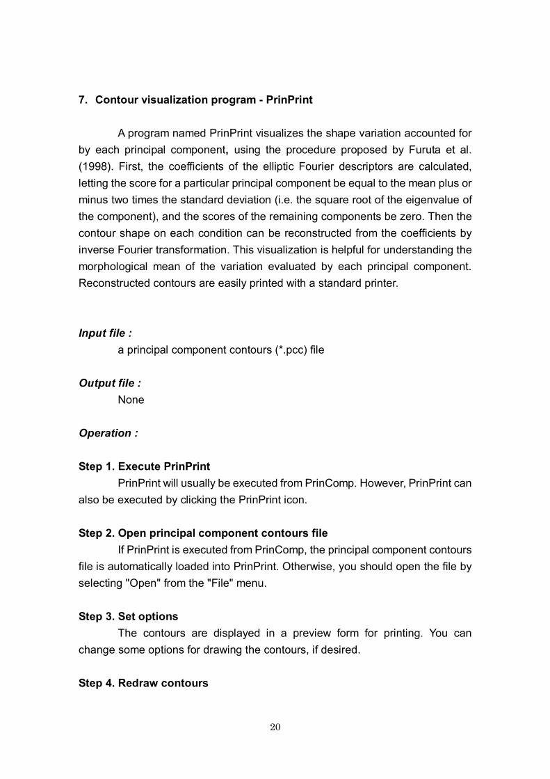
7. Contour visualization program ­ PrinPrint

A program named PrinPrint visualizes the shape variation accounted for by each principal component, using the procedure proposed by Furuta et al. (1998). First, the coefficients of the elliptic Fourier descriptors are calculated, letting the score for a particular principal component be equal to the mean plus or minus two times the standard deviation (i.e. the square root of the eigenvalue of the component), and the scores of the remaining components be zero. Then the contour shape on each condition can be reconstructed from the coefficients by inverse Fourier transformation. This visualization is helpful for understanding the morphological mean of the variation evaluated by each principal component. Reconstructed contours are easily printed with a standard printer.

Input file : a principal component contours (*.pcc) file

Output file : None

Operation :

Step 1. Execute PrinPrint PrinPrint will usually be executed from PrinComp. However, PrinPrint can

also be executed by clicking the PrinPrint icon.

Step 2. Open principal component contours file If PrinPrint is executed from PrinComp, the principal component contours

file is automatically loaded into PrinPrint. Otherwise, you should open the file by selecting "Open" from the "File" menu.

Step 3. Set options The contours are displayed in a preview form for printing. You can

change some options for drawing the contours, if desired.

Step 4. Redraw contours

21

After setting the draw options, click the "Redraw" button, the preview window will then be updated in accordance with the new settings.

Step 5. Print contours Select "Print" from the "File" menu or click the button with a printer icon,

and the print dialog will appear. After setting the printer properties, click the "OK" button. You can then print the contours.

22

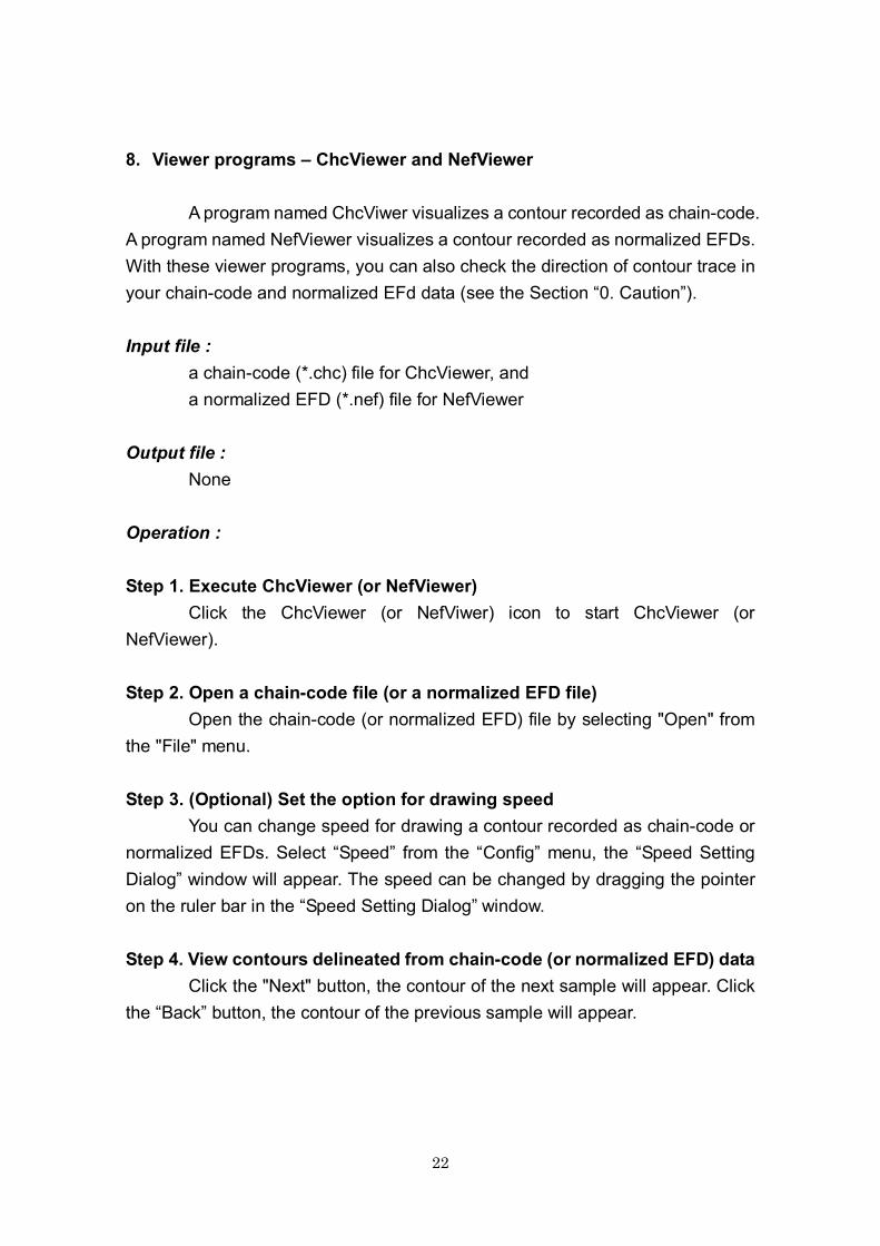
8. Viewer programs – ChcViewer and NefViewer

A program named ChcViwer visualizes a contour recorded as chain­code. A program named NefViewer visualizes a contour recorded as normalized EFDs. With these viewer programs, you can also check the direction of contour trace in your chain­code and normalized EFd data (see the Section “0. Caution”).

Input file : a chain­code (*.chc) file for ChcViewer, and a normalized EFD (*.nef) file for NefViewer

Output file : None

Operation :

Step 1. Execute ChcViewer (or NefViewer) Click the ChcViewer (or NefViwer) icon to start ChcViewer (or

NefViewer).

Step 2. Open a chain­code file (or a normalized EFD file) Open the chain­code (or normalized EFD) file by selecting "Open" from

the "File" menu.

Step 3. (Optional) Set the option for drawing speed You can change speed for drawing a contour recorded as chain­code or

normalized EFDs. Select “Speed” from the “Config” menu, the “Speed Setting Dialog” window will appear. The speed can be changed by dragging the pointer on the ruler bar in the “Speed Setting Dialog” window.

Step 4. View contours delineated from chain­code (or normalized EFD) data Click the "Next" button, the contour of the next sample will appear. Click

the “Back” button, the contour of the previous sample will appear.

23

About sample files

This package contains three sample files. First, please try using ChainCoder with "Sample_img.bmp". This file contains images of five radish roots and a 50 mm by 50 mm scale marker at the top. Next, try out Chc2Nef with "Sample_chc.chc" or a chain­code file made from "Sample_img.bmp" using ChainCoder. Finally, try using PrinComp and PrinPrint with "Sample_nef.nef" (this file contains sufficient data for principal component analysis). You can view contours recorded in “Sample_chc.chc” (or “Sample_nef.nef”) file by using ChcViewer (or NefViewer).

The tutorial (Tutorial.pdf) included in this package will help you to try out SHAPE with the sample files.

24

9. How to cite SHAPE

When you intend to publish results from SHAPE, please cite SHAPE as follows:

Iwata, H. and Y. Ukai (2002) SHAPE: A computer program package for quantitative evaluation of biological shapes based on elliptic Fourier descriptors. Journal of Heredity 93: 384­385

10.Acknowledgements

I would like to thank Prof. Yasuo Ukai for suggesting that I develop this software package and for giving me constant guidance. I would also like to thank Mr. Naoya Furuta, and Drs. Hiroshi Ohmori, Takeshi Hayashi, Yasushi Takano and Seishi Ninomiya for valuable suggestions about elliptic Fourier analysis, statistical analysis and computer programming.

25

11.References

Bierbaum RM and Ferson S, 1986. Do symbiotic pea crabs decrease growth rate in mussels? Biol Bull 170: 51­61.

Diaz G, Zuccarelli A, Pelligra I and Ghiani A, 1989. Elliptic Fourier analysis of cell and nuclear shapes. Comp Biomed Res 22: 405­414.

Ferson S, Rohlf FJ and Koehn RK, 1985. Measuring shape variation of two­dimensional outlines. Syst Zool 34: 59­68.

Freeman H, 1974. Computer processing of line drawing images, Comp Surv 6: 57­97.

Furuta N, Ninomiya S, Takahashi S, Ohmori H and Ukai Y, 1995. Quantitative evaluation of soybean (Glycine max L., Merr.) leaflet shape by principal component scores based on elliptic Fourier descriptor. Breed Sci 45: 315­320.

Iwata H, Nesumi H, Ninomiya S, Takano Y and Ukai Y, 2002. Diallel analysis of leaf shape variations of citrus varieties based on elliptic Fourier descriptors. Breeding Science 52: 89­94.

Iwata H, Niikura S, Matsuura S, Takano Y and Ukai Y, 1998. Evaluation of variation of root shape of Japanese radish (Raphanus sativus L.) based on image analysis using elliptic Fourier descriptors. Euphytica 102: 143­149.

Iwata H, Niikura S, Matsuura S, Takano Y and Ukai Y, 2000. Diallel analysis of root shape of Japanese radish (Raphanus sativus L.) based on elliptic Fourier descriptors. Breed Sci 50: 73­80.

Iwata H, Niikura S, Matsuura S, Takano Y and Ukai Y, 2004a. Genetic control of root shape at different growth stages in radish (Raphanus sativus L.). Breeding Science 54: 117­124.

Iwata H, Niikura S, Matsuura S, Takano Y, and Ukai Y, 2004b. Interaction between genetic effects by soil type in diallel analysis of root shape and size of Japanese radish (Raphanus sativus L.). Breeding Science 54: 313­318.

Iwata H. and Ukai Y, (2002) SHAPE: A computer program package for quantitative evaluation of biological shapes based on elliptic Fourier descriptors. Journal of Heredity 93: 384­385.

Kuhl FP and Giardina CR, 1982. Elliptic Fourier features of a closed contour. Comp Graph Ima Proc 18: 236­258.

26

Laurie CC, True JR, Liu J and Mercer JM, 1997. An introgression analysis of quantitative trait loci that contribute to a morphological difference between Drosophila simulans and D. mauritiana. Genetics 145: 339­348.

Liu J, Mercer JM, Stam LF, Gibson G and Laurie CC, 1996. Genetic analysis of a morphological shape difference in the male genitalia of Drosophila simulans and D. mauritiana. Genetics 142: 1129­1145.

McLellan T, 1993. The roles of heterochrony and heteroblasty in the diversification of leaf shapes in Begonia dregei (Begoniaceae). Am J Bot 80: 796­804.

Ohsawa R, Tsutsumi T, Uehara H, Namai H and Ninomiya S, 1998. Quantitative evaluation of common buckwheat (Fagopyrum esculentum Moench) kernel shape by elliptic Fourier descriptor. Euphytica 101: 175­183.

Rohlf FJ and Archie JW, 1984. A comparison of Fourier methods for the description of wing shape in mosquitoes (Ritera culicidae). Syst Zool 33: 302­317.

Toyohara H, Irie K, Ding W, Iwata H, Fujimaki H, Kikuchi F and Ukai Y, 2000. Evaluation of tuber shape of yam (Dioscorea alta L.) cultivars by image analysis and elliptic Fourier descriptors. SABRAO J Breed. Genet. 32: 31­37.

Uga Y, Fukuta Y, Cai HW, Iwata H, Ohsawa R, Morishima H, Fujimura T, 2003. Mapping QTLs influencing rice floral morphology using recombinant inbred lines derived from a cross between Oryza sativa L. and O. rufipogon Griff. Theoretical and Applied Genetics 107: 218­226.

White R, Rentice HC, Verwist T, (1988) Automated image acquisition and morphometric description. Can J Bot 66: 450­459.

Yoshioka Y, Iwata H, Ohsawa R, Ninomiya S, 2005a. Quantitative evaluation of flower colour pattern by image analysis and principal component analysis of Primula sieboldii E. Morren. Euphytica 139: 179­186.

Yoshioka Y, Iwata H, Ohsawa R, Ninomiya S, 2005b. Quantitative evaluation of the petal shape variation in Primula sieboldii caused by breeding process in the last 300 years. Heredity 94: 657­663.

Yoshioka Y, Iwata H, Fukuta N, Ohsawa R, Ninomiya S, 2006a. Quantitative evaluation of petal shape and picotee color pattern in lisianthus by image analysis. Journal of the American Society for Horticultural Science 131: 261­266.

27

Yoshioka Y, Iwata H, Hase N, Matsuura S, Ohsawa R, Ninomiya S, 2006b. Genetic combining ability of petal shape in garden pansy (Viola x wittrockiana Gams) based on image analysis. Euphytica 151: 311­319

28

12.Appendix

Elliptic Fourier descriptors

The coefficients of elliptic Fourier descriptors are calculated by the discrete Fourier transformation of chain­coded contours through the procedure proposed by Kuhl and Giardina (1982). Briefly, the procedure is as follows:

A contour of the digitized shapes can be represented as a sequence of the x­ and y­ coordinates of ordered points measured contour­clockwise from an arbitrary starting point. Assuming that the contour between two adjacent points is linearly interpolated, and the length of the linear segment between the (i ­ 1)th and the ith points is i t ∆ , then the length of the contour from the starting point to

the pth point is ∑ = ∆ = ∆ p

i i p t t 1

, and the perimeter of the contour is K t T = , where K

is the total number of the points on the contour. Note that the Kth point is

equivalent to the starting point. The x­ coordinate of the pth point is ∑ = ∆ = p

i i p x x 1

,

where i x ∆ is the displacement along the x­ axis of the contour between the (i­1)th and ith points. Then, elliptic Fourier expansion of the sequences of the x­coordinates gives

∑ ∞

=

+ + = 1

) 2

sin 2

cos ( n

p n

p n cen p T

t n b

T t n

a x x π π

,

where

∑=

− − ∆

∆ =

K

p

p p

p

p n T

t n T t n

t x

n T a

1

1 2 2 )

2 cos

2 (cos

2 π π

π ,

and

∑=

− − ∆

∆ =

K

p

p p

p

p n T

t n T t n

t x

n T b

1

1 2 2 )

2 sin

2 (sin

2 π π

π .

In the above equation, cen x is the coordinate of the center point, and n is the harmonic number of the coefficients ( n a and n b ). The coefficients values for the y­ coordinates, n c and n d , are found in the same way.

The coefficients of elliptic Fourier descriptors can be mathematically normalized to be invariant to size, rotation and starting point of the contour trace. In SHAPE, the coefficients can be normalized by two types of procedures; one

29

based on the ellipse of the first harmonic and the other based on the longest radius. For detailed information about the normalization, see Kuhl and Giardina (1982).