Sharpe-optimal SPDR portfoliosor

How to beat the marketand sleep well at night

byVic Norton

Bowling Green, Ohio 43402-2223USA

<mailto:vic@norton.name>

Website<http://vic.norton.name/

finance-math/sospdr/>

1

Sharpe Ratio

The Sharpe Ratio of an investment is the ratio of itsexpected reward to its risk.

1990 Nobel Prize in Economics.

Harry Markowitz (U.S.) Baruch College (of theCity Univ. of New York), for his Portfolio The-ory. William F. Sharpe (U.S.) Stanford Univ., forhis Capital Asset Pricing Model. Merton Miller(U.S.) Univ. of Chicago, for his work on the Miller-Modigliani Theory.

Together, their work revolutionized the finan-cial/business industries.

– 2006 New York Times Almanac

2

Select Sector SPDRs

The Select Sector SPDRs (pronounced ”spiders”)are ETFs (Exchange Traded Funds) that partition theS&P 500 (U.S. large-cap stocks) into 9 categories:

XLY – Consumer DiscretionaryXLP – Consumer StaplesXLE – EnergyXLF – FinancialXLV – Health CareXLI – IndustrialXLB – MaterialsXLK – TechnologyXLU – Utilities

Problem: Determine a portfolio in these SPDRs thatmaximizes the ratio of expected reward to risk, the“Sharpe Ratio.”

Strategy for beating the market and sleeping well atnight: Every now and then reinvest in the ex post,Sharpe-optimal portfolio, deleveraging with the basefund as appropriate. (More details on the “sospdr”web site.)

3

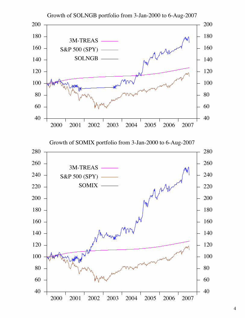
4

Abstract

The Sharpe Ratio of an investment portfolio is,loosely speaking, the ratio of its reward to its risk.We seek portfolios of maximum Sharpe Ratio froma fixed universe of Exchange Traded Funds (ETFs,Select Sector SPDRs).

It is convenient to look at this problem in a geomet-ric setting. Then a portfolio is identified with its riskvector in a high-dimensional Euclidean space, andthe Sharpe Ratio of the portfolio is proportional tothe cosine of the angle between the risk vector andan expected-reward axis. Now we seek to maximizethis cosine (and thus the Sharpe Ratio) over a convexpolytope of portfolios. The maximization is accom-plished by a simplex-type algorithm using updatedQR-factorizations.

5

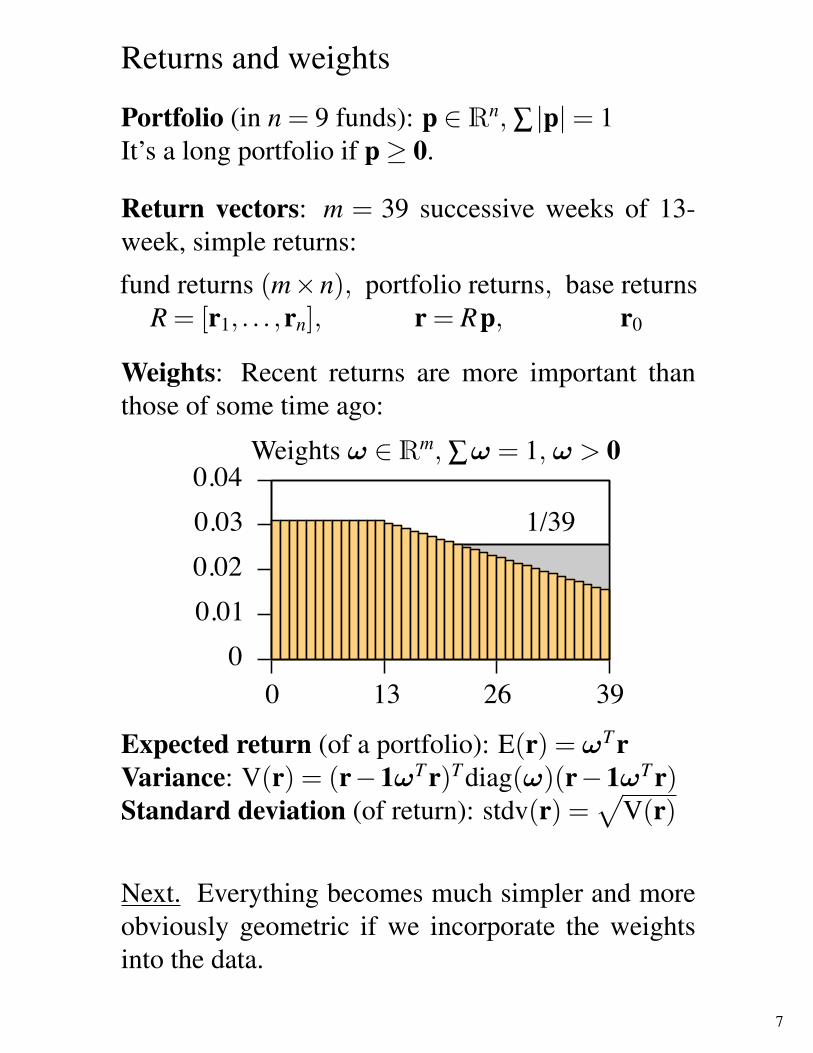
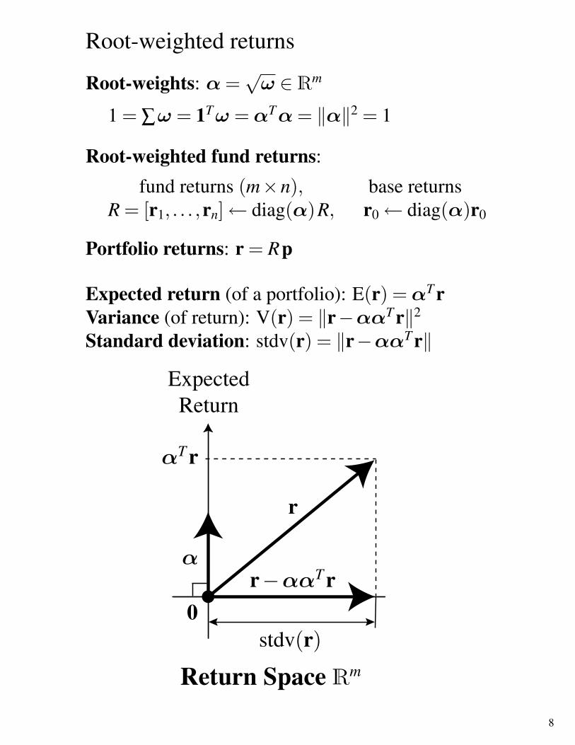
Data

Computations depend on data.

We use historical, adjusted-price data for various se-curities from Yahoo Finance

<http://finance.yahoo.com/>and interest rate data from the Federal Reserve

<http://federalreserve.gov/

Releases/h15/data.htm>.

These data are freely available to anyone.

6

Returns and weights

Portfolio (in n = 9 funds): p ∈Rn, ∑ |p|= 1It’s a long portfolio if p≥ 0.

Return vectors: m = 39 successive weeks of 13-week, simple returns:

fund returns (m×n), portfolio returns, base returnsR = [r1, . . . ,rn], r = Rp, r0

Weights: Recent returns are more important thanthose of some time ago:

Weights ω ∈Rm, ∑ω = 1, ω > 0

Expected return (of a portfolio): E(r) = ωT rVariance: V(r) = (r−1ωT r)T diag(ω)(r−1ωT r)Standard deviation (of return): stdv(r) =

√V(r)

Next. Everything becomes much simpler and moreobviously geometric if we incorporate the weightsinto the data.

7

Root-weighted returns

Root-weights: α=√ω ∈Rm

1 = ∑ω = 1Tω =αTα= ‖α‖2 = 1

Root-weighted fund returns:

fund returns (m×n), base returnsR = [r1, . . . ,rn]← diag(α)R, r0← diag(α)r0

Portfolio returns: r = Rp

Expected return (of a portfolio): E(r) =αT rVariance (of return): V(r) = ‖r−ααT r‖2

Standard deviation: stdv(r) = ‖r−ααT r‖

ExpectedReturn

Return Space8

Rewards

Fund reward vectors: w j = r j− r0 ∈Rm

W = [w1, . . . ,wn] = R− r01T ∈Rm×n

Portfolio reward vector: w = Wp

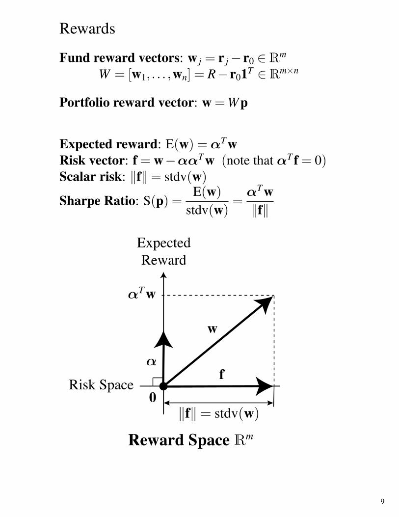
Expected reward: E(w) =αT wRisk vector: f = w−ααT w (note that αT f = 0)Scalar risk: ‖f‖= stdv(w)

Sharpe Ratio: S(p) =E(w)

stdv(w)=αT w‖f‖

ExpectedReward

Risk Space

Reward Space

9

Risks

Fund risk vectors: f j = w j!!!T w j "Rm

F = [f1, . . . , fn] = (I!!!T)W "Rm#n

Portfolio risk: f = Fp, scalar risk: $f$

Expected reward vector: e = F(FT F)!1ET

where E = [E(w1), . . . ,E(w1)] = !TWProperties1. e is a risk vector: !T e = 0.2. eT F = E. (Expected reward is a function of risk)3. The Sharpe Ratio of the portfolio p is given by

S(p) =eT f$f$ = $e$cosu(f), u = e/$e$,

where cosu(f) = (uT f)/$f$ for f %= 0.

Asset allocation problem. Find a long portfolio pin n funds of maximal Sharpe Ratio.

Corresponding mathematical problem. Given anm#n matrix F and a unit m-vector u, find a point

f = Fp, !p = 1, p& 0,

that maximizes cosu on the convex hull of thecolumns of F .

10

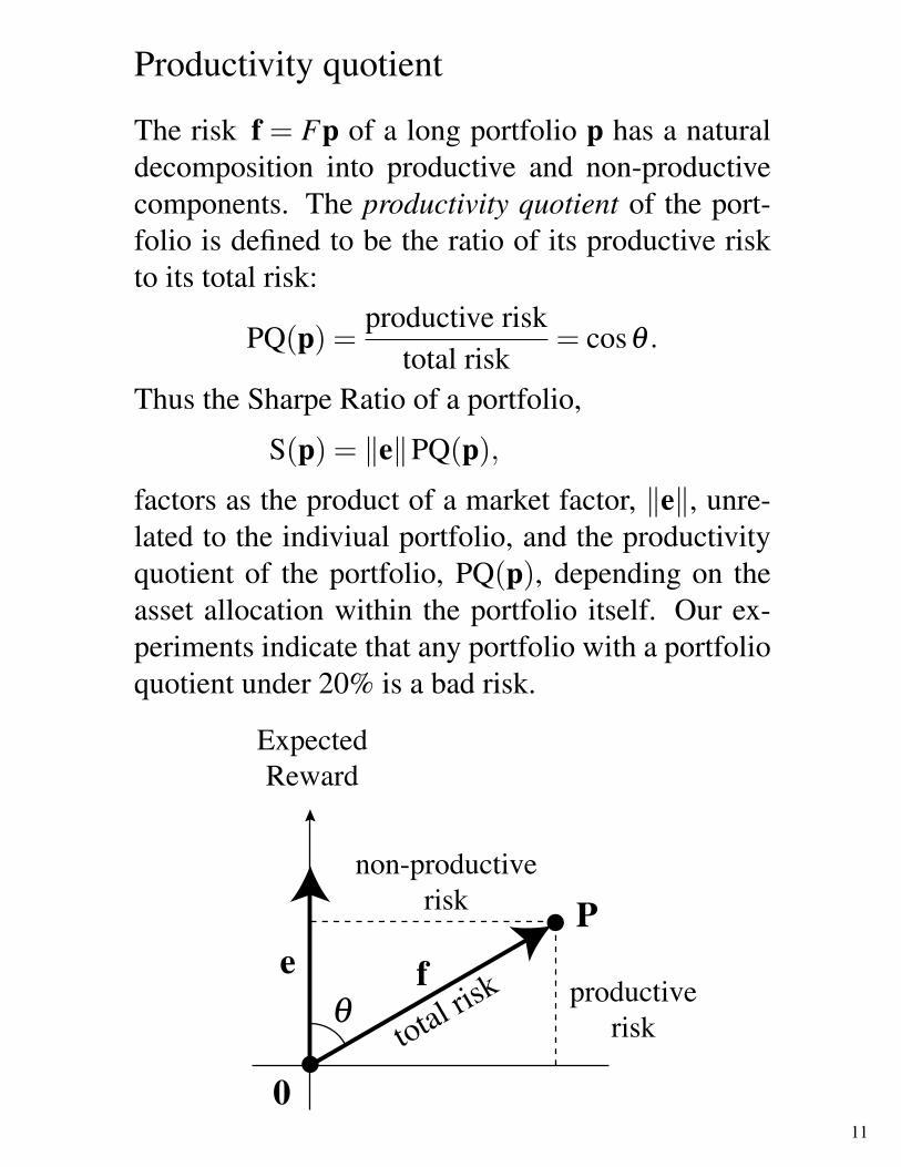
Productivity quotient

The risk f = Fp of a long portfolio p has a naturaldecomposition into productive and non-productivecomponents. The productivity quotient of the port-folio is defined to be the ratio of its productive riskto its total risk:

PQ(p) =productive risk

total risk= cosθ .

Thus the Sharpe Ratio of a portfolio,

S(p) = ‖e‖PQ(p),

factors as the product of a market factor, ‖e‖, unre-lated to the indiviual portfolio, and the productivityquotient of the portfolio, PQ(p), depending on theasset allocation within the portfolio itself. Our ex-periments indicate that any portfolio with a portfolioquotient under 20% is a bad risk.

non-productiverisk

productiverisktotal ris

k

ExpectedReward

11

Summary of part 1

Any long portfolio in the 9 risky funds (the Se-lect Sector SPDRs) has a risk vector that is aconvex combination of the fund risk vectors. Theexpected reward of the portfolio is the dot prod-uct of its risk vector with the expected rewardvector. The risk of the portfolio (its standard de-viation of reward) is the length of its risk vec-tor. Thus the Sharpe ratio of the portfolio is afixed multiple of the cosine of the angle betweenits risk vector and the expected reward axis. Tomaximize the Sharpe ratio we need to minimizethis angle (and maximize its cosine).

summary of part 1

How to maximize a cosine

byVic Norton

Bowling Green, Ohio 43402-2223USA

<mailto:vic@norton.name>

Website<http://vic.norton.name/

finance-math/maxcos/>

12

Abstract

Given a unit m-vector u and a nonzero m× n ma-trix A, we describe a simplex-type algorithm to max-imize the cosine function

cosu(P) = (uT P)/‖P‖

on the convex hull of the columns of A. The maxi-mizing P is returned in the form

Pmax = AJ p ,

where J is a sequence of nJ distinct indices from{1, . . . ,n}, the nJ columns of AJ are linearly indepen-dent, and p is an nJ-vector satisfying ∑p = 1, p > 0.

13

Some Notation

A = [a1, . . . ,an] ∈Rm×n, “the vertices”

J = [ j1, . . . , jnJ], nJ distinct indices from {1, . . . ,n}AJ = [a j1, . . . ,a jnJ

], linearly independentAJ = QR, QR-decomposition:

QTQ = I, R upper triangular, nonsingular

C (AJ) – the convex hull of the columns of AJ

F (AJ) – the flat spanned by the columns of AJ

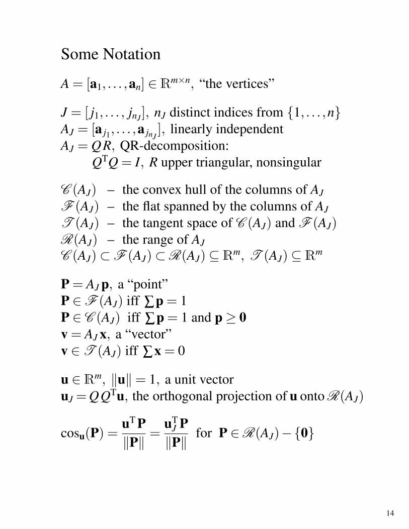
T (AJ) – the tangent space of C (AJ) and F (AJ)R(AJ) – the range of AJC (AJ)⊂F (AJ)⊂R(AJ)⊆Rm, T (AJ)⊆Rm

P = AJ p, a “point”P ∈F (AJ) iff ∑p = 1P ∈ C (AJ) iff ∑p = 1 and p≥ 0v = AJ x, a “vector”v ∈T (AJ) iff ∑x = 0

u ∈Rm, ‖u‖= 1, a unit vectoruJ = QQTu, the orthogonal projection of u onto R(AJ)

cosu(P) =uT P‖P‖

=uT

J P‖P‖

for P ∈R(AJ)−{0}

14

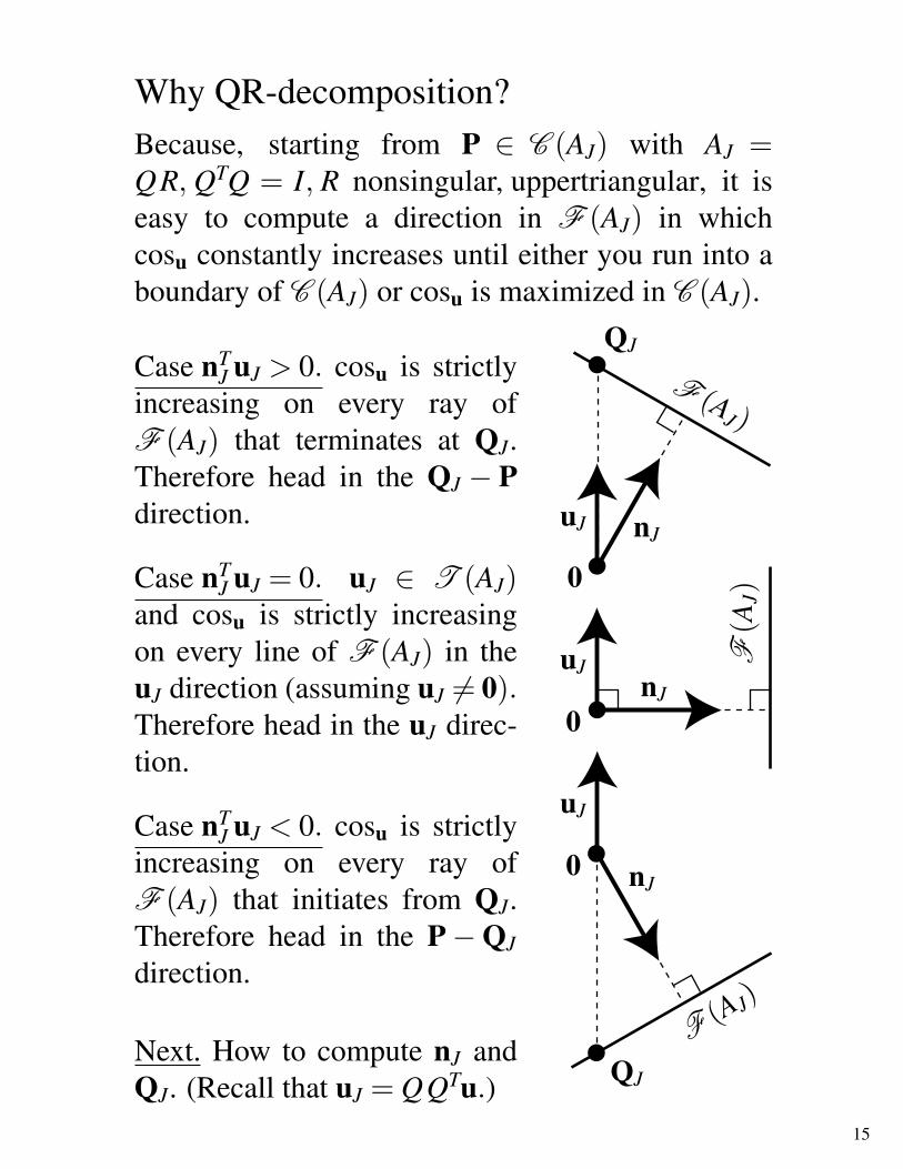
Why QR-decomposition?Because, starting from P ∈ C (AJ) with AJ =QR, QTQ = I, R nonsingular, uppertriangular, it iseasy to compute a direction in F (AJ) in whichcosu constantly increases until either you run into aboundary of C (AJ) or cosu is maximized in C (AJ).

Case nTJ uJ > 0. cosu is strictly

increasing on every ray ofF (AJ) that terminates at QJ.Therefore head in the QJ − Pdirection.

Case nTJ uJ = 0. uJ ∈ T (AJ)

and cosu is strictly increasingon every line of F (AJ) in theuJ direction (assuming uJ 6= 0).Therefore head in the uJ direc-tion.

Case nTJ uJ < 0. cosu is strictly

increasing on every ray ofF (AJ) that initiates from QJ.Therefore head in the P−QJ

direction.

Next. How to compute nJ andQJ. (Recall that uJ = QQTu.)

15

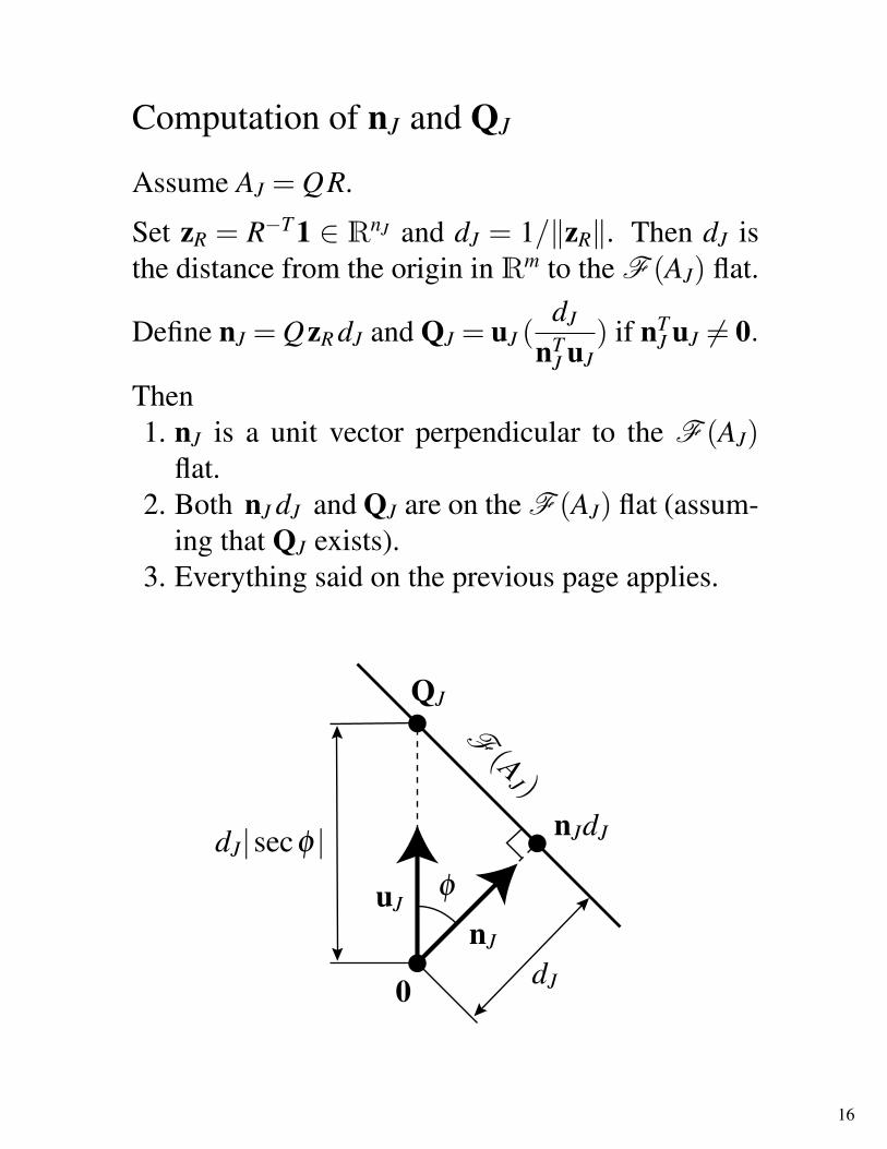
Computation of nJ and QJ

Assume AJ = QR.

Set zR = R−T 1 ∈ RnJ and dJ = 1/‖zR‖. Then dJ isthe distance from the origin in Rm to the F (AJ) flat.

Define nJ = QzR dJ and QJ = uJ (dJ

nTJ uJ

) if nTJ uJ 6= 0.

Then1. nJ is a unit vector perpendicular to the F (AJ)

flat.2. Both nJ dJ and QJ are on the F (AJ) flat (assum-

ing that QJ exists).3. Everything said on the previous page applies.

16

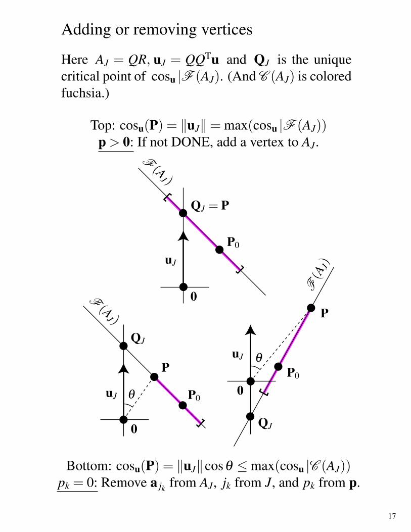
Adding or removing vertices

Here AJ = QR, uJ = QQTu and QJ is the uniquecritical point of cosu |F (AJ). (And C (AJ) is coloredfuchsia.)

Top: cosu(P) = ‖uJ‖= max(cosu |F (AJ))p > 0: If not DONE, add a vertex to AJ.

Bottom: cosu(P) = ‖uJ‖cosθ ≤max(cosu |C (AJ))pk = 0: Remove a jk from AJ, jk from J, and pk from p.

17

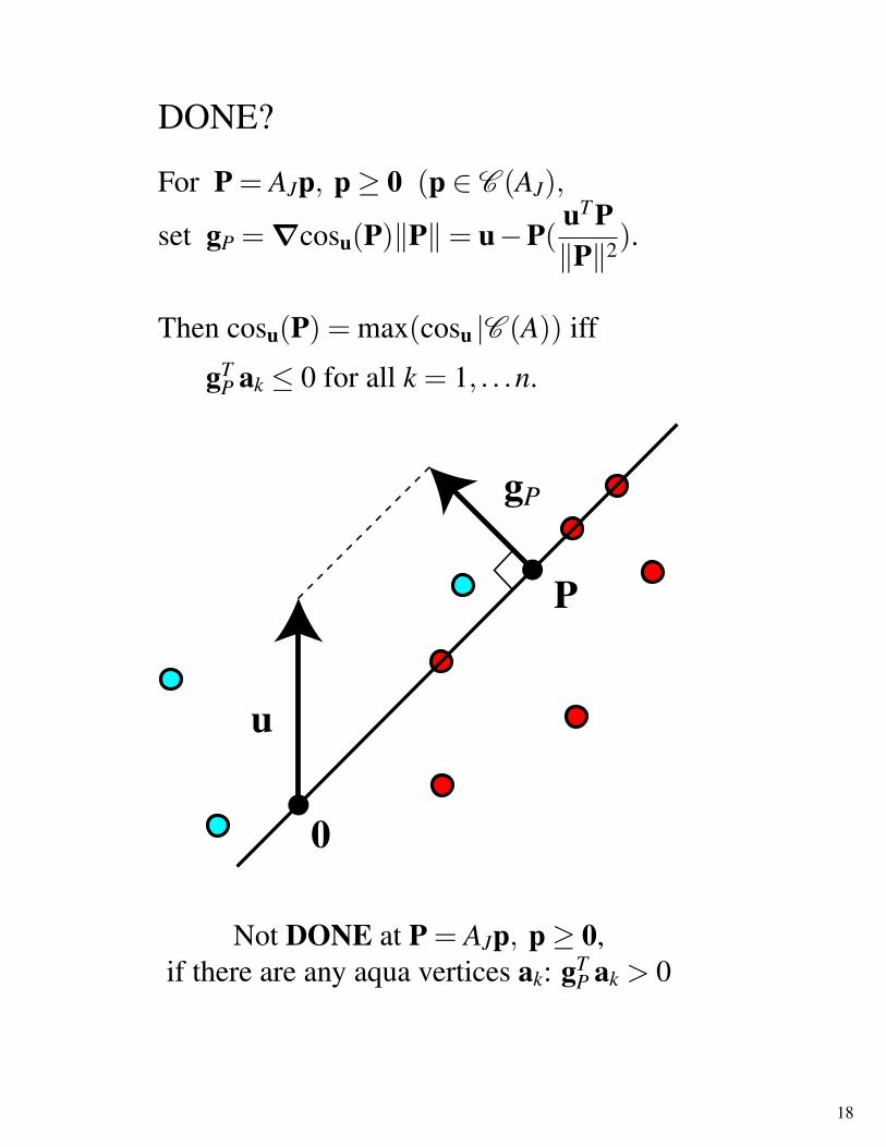
DONE?

For P = AJp, p≥ 0 (p ∈ C (AJ),

set gP = ∇cosu(P)‖P‖= u−P(uT P‖P‖2).

Then cosu(P) = max(cosu |C (A)) iff

gTP ak ≤ 0 for all k = 1, . . .n.

Not DONE at P = AJp, p≥ 0,if there are any aqua vertices ak: gT

P ak > 0

18

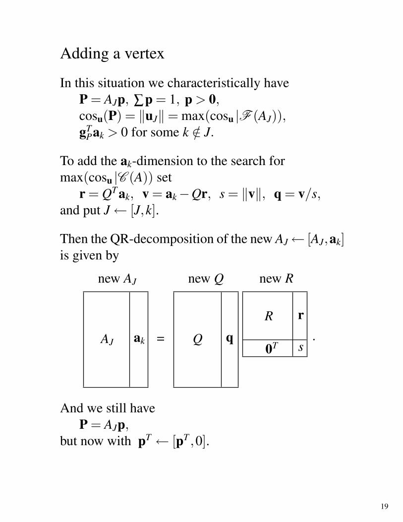
Adding a vertex

In this situation we characteristically haveP = AJp, ∑p = 1, p > 0,cosu(P) = ‖uJ‖= max(cosu |F (AJ)),gT

Pak > 0 for some k /∈ J.

To add the ak-dimension to the search formax(cosu |C (A)) set

r = QT ak, v = ak−Qr, s = ‖v‖, q = v/s,and put J← [J,k].

Then the QR-decomposition of the new AJ← [AJ,ak]is given by

AJ ak = Q qR

0T

r

s

new AJ new Q new R

.

And we still haveP = AJp,

but now with pT ← [pT ,0].

19

Givens rotation

A rotation of an orthonormal basis of a plane thatzeros the second coordinate of a given vector.

v = [q1 q2]!!!

"= [#q1 #q2]

!!0

"

!qT

1qT

2

"[q1 q2] =

!#qT

1#qT

2

"[#q1 #q2] =

!1 00 1

"

givens

G =!

c "ss c

",

c = cos!s = sin!

rot.col rot.row

[#q1 #q2] = [q1 q2]G, GT!! · · ·! · · ·

"=

!! · · ·0 · · ·

"

20

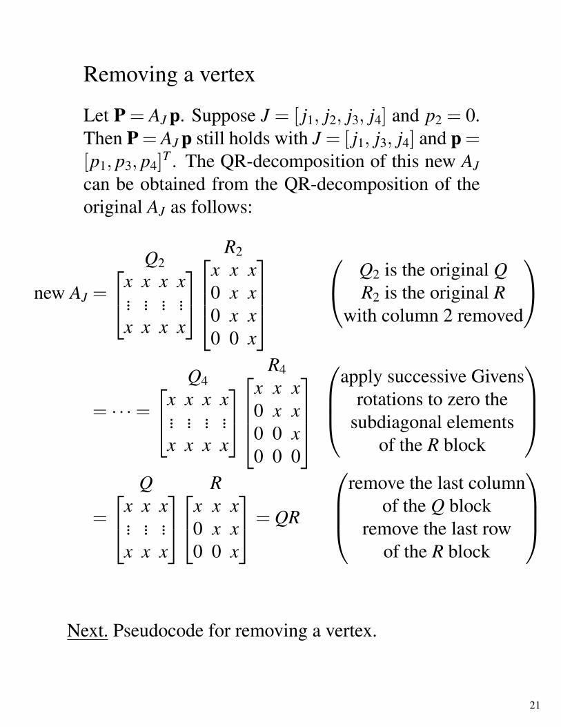
Removing a vertex

Let P = AJ p. Suppose J = [ j1, j2, j3, j4] and p2 = 0.Then P = AJ p still holds with J = [ j1, j3, j4] and p =[p1, p3, p4]T . The QR-decomposition of this new AJ

can be obtained from the QR-decomposition of theoriginal AJ as follows:

new AJ =

Q2x x x x... ... ... ...x x x x

R2

x x x0 x x0 x x0 0 x

Q2 is the original Q

R2 is the original Rwith column 2 removed

= · · ·=

Q4x x x x... ... ... ...x x x x

R4

x x x0 x x0 0 x0 0 0

apply successive Givensrotations to zero the

subdiagonal elementsof the R block

=

Qx x x... ... ...x x x

Rx x x

0 x x0 0 x

= QR

remove the last column

of the Q blockremove the last row

of the R block

Next. Pseudocode for removing a vertex.

21

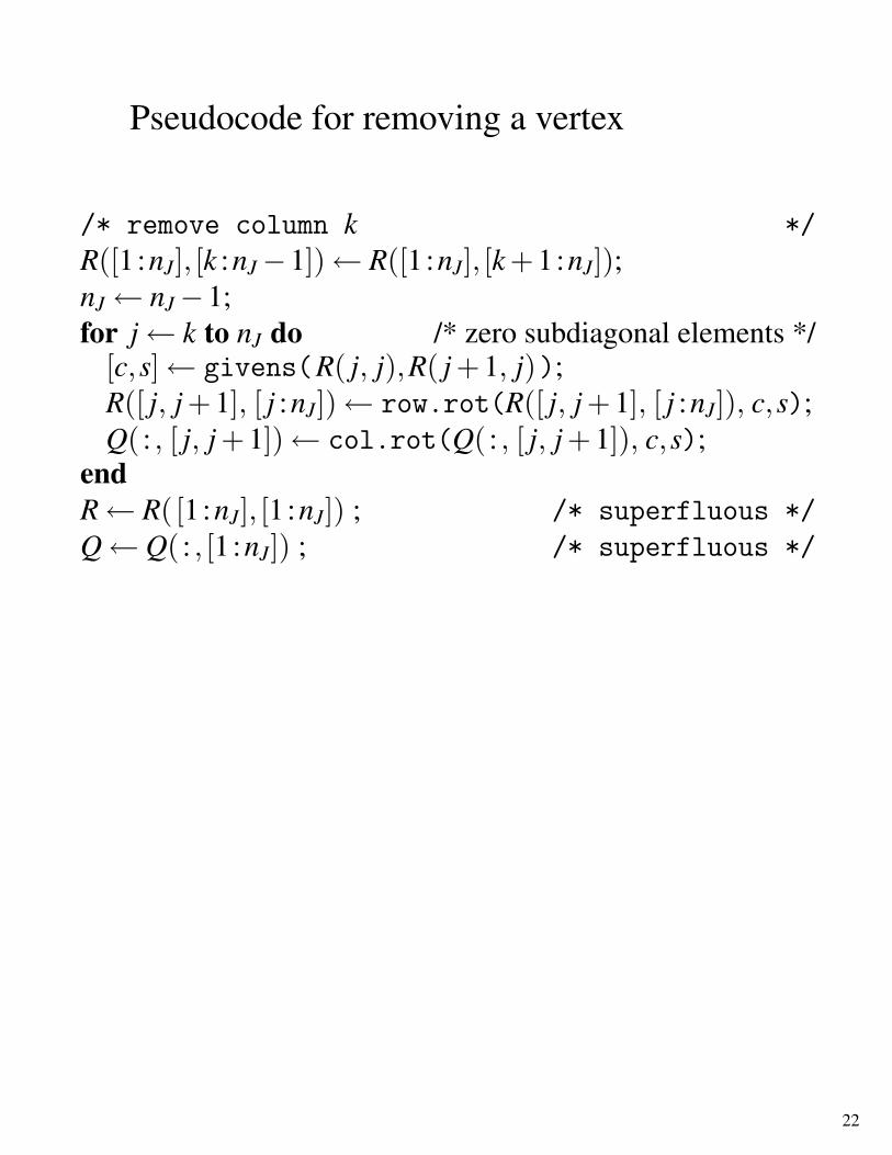
Pseudocode for removing a vertex

/* remove column k */

R([1:nJ], [k :nJ−1])← R([1:nJ], [k +1:nJ]);nJ← nJ−1;for j← k to nJ do /* zero subdiagonal elements */

[c,s]← givens(R( j, j),R( j +1, j));R([ j, j +1], [ j :nJ])← row.rot(R([ j, j +1], [ j :nJ]), c,s);Q( : , [ j, j +1])← col.rot(Q( : , [ j, j +1]), c,s);

endR← R( [1:nJ], [1:nJ]) ; /* superfluous */

Q← Q( : , [1:nJ]) ; /* superfluous */

22

To maximize cosu |C (A):1. Start at vertex A : AJ = [A].

2. Add vertex B : AJ = [A,B].

3. Proceed to P1 = max(cosu |C (AJ)).

4. Add vertex C : AJ = [A,B,C].

5. Proceed directly towardQ = max(cosu |F (AJ)) until you hit theboundary of C (AJ) at P2.

6. Remove vertex A : AJ = [B,C].

7. Proceed to P3 = max(cosu |C (AJ)).

23

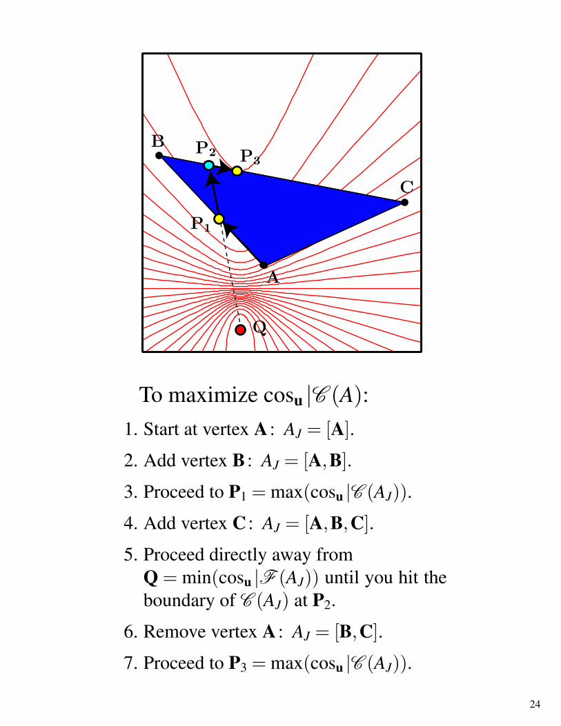
To maximize cosu |C (A):1. Start at vertex A : AJ = [A].

2. Add vertex B : AJ = [A,B].

3. Proceed to P1 = max(cosu |C (AJ)).

4. Add vertex C : AJ = [A,B,C].

5. Proceed directly away fromQ = min(cosu |F (AJ)) until you hit theboundary of C (AJ) at P2.

6. Remove vertex A : AJ = [B,C].

7. Proceed to P3 = max(cosu |C (AJ)).

24

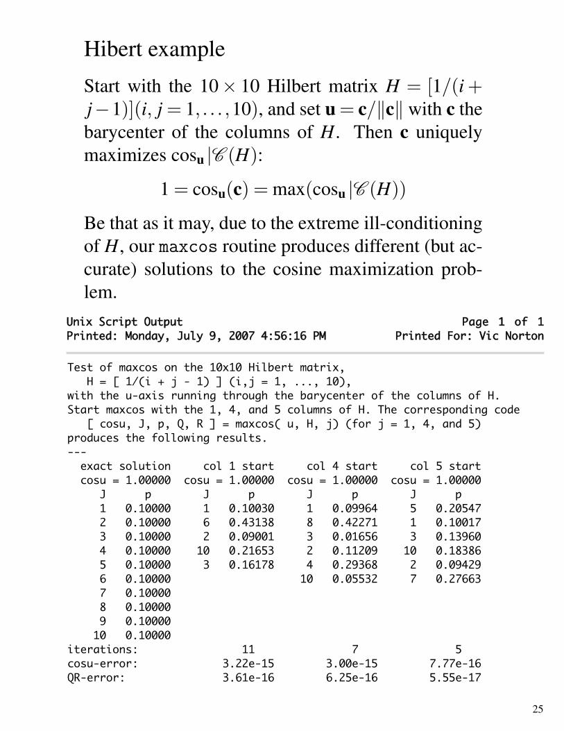
Hibert example

Start with the 10× 10 Hilbert matrix H = [1/(i +j−1)](i, j = 1, . . . ,10), and set u = c/‖c‖ with c thebarycenter of the columns of H. Then c uniquelymaximizes cosu |C (H):

1 = cosu(c) = max(cosu |C (H))

Be that as it may, due to the extreme ill-conditioningof H, our maxcos routine produces different (but ac-curate) solutions to the cosine maximization prob-lem.

Page 1 of 1Unix Script OutputPrinted: Monday, July 9, 2007 4:56:16 PM Printed For: Vic Norton

Test of maxcos on the 10x10 Hilbert matrix, H = [ 1/(i + j - 1) ] (i,j = 1, ..., 10),with the u-axis running through the barycenter of the columns of H.Start maxcos with the 1, 4, and 5 columns of H. The corresponding code [ cosu, J, p, Q, R ] = maxcos( u, H, j) (for j = 1, 4, and 5)produces the following results.--- exact solution col 1 start col 4 start col 5 start cosu = 1.00000 cosu = 1.00000 cosu = 1.00000 cosu = 1.00000 J p J p J p J p 1 0.10000 1 0.10030 1 0.09964 5 0.20547 2 0.10000 6 0.43138 8 0.42271 1 0.10017 3 0.10000 2 0.09001 3 0.01656 3 0.13960 4 0.10000 10 0.21653 2 0.11209 10 0.18386 5 0.10000 3 0.16178 4 0.29368 2 0.09429 6 0.10000 10 0.05532 7 0.27663 7 0.10000 8 0.10000 9 0.10000 10 0.10000 iterations: 11 7 5 cosu-error: 3.22e-15 3.00e-15 7.77e-16QR-error: 3.61e-16 6.25e-16 5.55e-17

25