University of Kentucky University of Kentucky UKnowledge UKnowledge University of Kentucky Master's Theses Graduate School 2006 Shear-Wave Velocities and Derivative Mapping For the Upper Shear-Wave Velocities and Derivative Mapping For the Upper Mississippi Embayment Mississippi Embayment David M. Vance University of Kentucky, [email protected]Right click to open a feedback form in a new tab to let us know how this document benefits you. Right click to open a feedback form in a new tab to let us know how this document benefits you. Recommended Citation Recommended Citation Vance, David M., "Shear-Wave Velocities and Derivative Mapping For the Upper Mississippi Embayment" (2006). University of Kentucky Master's Theses. 296. https://uknowledge.uky.edu/gradschool_theses/296 This Thesis is brought to you for free and open access by the Graduate School at UKnowledge. It has been accepted for inclusion in University of Kentucky Master's Theses by an authorized administrator of UKnowledge. For more information, please contact [email protected].
Transcript
University of Kentucky University of Kentucky
UKnowledge UKnowledge
University of Kentucky Master's Theses Graduate School
2006
Shear-Wave Velocities and Derivative Mapping For the Upper Shear-Wave Velocities and Derivative Mapping For the Upper
Right click to open a feedback form in a new tab to let us know how this document benefits you. Right click to open a feedback form in a new tab to let us know how this document benefits you.
Recommended Citation Recommended Citation Vance, David M., "Shear-Wave Velocities and Derivative Mapping For the Upper Mississippi Embayment" (2006). University of Kentucky Master's Theses. 296. https://uknowledge.uky.edu/gradschool_theses/296
This Thesis is brought to you for free and open access by the Graduate School at UKnowledge. It has been accepted for inclusion in University of Kentucky Master's Theses by an authorized administrator of UKnowledge. For more information, please contact [email protected].
Shear-Wave Velocities and Derivative Mapping For the Upper Mississippi Embayment
During the past two decades, University of Kentucky researchers have been acquiring seismic refraction/reflection data, as well as seismic downhole data, for characterizing the seismic velocity models of the soil/sediment overburden in the central United States. The dataset includes densely spaced measurements for urban microzonation studies and coarsely spaced measurements for regional assessments. The 519 measurements and their derivative products often were not in an organized electronic form, however, limiting their accessibility for use by other researchers. In order to make these data more accessible, this project constructed a database using the ArcGIS 9.1 software. The data have been formatted and integrated into a system serving a wider array of users. The seismic shear-wave velocity models collected at various locations are archived with corresponding x-, y-, and z-coordinate information. Flexibility has been included to allow input of additional data in the future (e.g., seismograms, strong ground-motion parameters and time histories, weak-motion waveform data, etc.). Using the completed database, maps of the region showing derivative dynamic site period (DSP) and weighted shear-wave velocity of the upper 30 m of soil (V30) were created using the ArcGIS 9.1 Geostatistical Analyst extension for examination of the distribution of pertinent dynamic properties for seismic hazard assessments. Both geostatistical and deterministic techniques were employed. Interpolation of V30 data yielded inaccurate predictions because of the high lateral variation in soil layer lithology in the Jackson Purchase Region. As a result of the relatively uniform distribution of depths to bedrock, the predictions of DSP values suggested a high degree of accuracy.
Keywords: GIS, geodatabase, kriging, shear-wave velocity, dynamic site period
Shear-Wave Velocity Database and Derivative Mapping For the Upper Mississippi Embayment
By
David M. Vance
Dr. Edward W. Woolery Director of Thesis Dr. Sue Rimmer Director of Graduate Studies
Rules for the Use of Thesis
Unpublished theses submitted for the Master’s degree and deposited in the University of Kentucky Library are as a rule open for inspection, but are to be used only with due regard to the rights of the authors. Bibliographical references may be noted, but quotations or summaries of parts may be published only with the permission of the author, and with the usual scholarly acknowledgements. Extensive copying or publication of the thesis in whole or in part also requires the consent of the Dean of the Graduate School of the University of Kentucky. A library that borrows this thesis for use by its patrons is expected to secure the signature of each user.
THESIS
David M. Vance
The Graduate School
University of Kentucky
2006
SHEAR-WAVE VELOCITY DATABASE AND DERIVATIVE MAPPING FOR THE UPPER MISSISSIPPI EMBAYMENT
THESIS
A thesis submitted in partial fulfillment of the requirements of the degree of Master of Science in the
College of Arts and Sciences at the University of Kentucky
By
David M. Vance
Director: Dr. Edward W. Woolery, University of Kentucky Department of Earth and Environmental Sciences
Acknowledgments The completion of this project would not have been possible without the support of many friends and colleagues. First, I’d like to thank the Kentucky Geological Survey for providing both financial and technical support. In particular, Jackie Silvers and Mandy Long were dependable sources of help throughout the process. Mark C. Thompson was invaluable in keeping the computer network and software available and running. I’d also like to thank Dr. Zhenming Wang and Dr. John Kiefer for excellent advice and suggestions concerning the development of this project. I appreciate the comments, insights, and suggestions of Josh Sexton, James Ward, James Whitt, and Ken Macpherson, as well. Dr. Ed Woolery, in addition to being my supervisor, has been an outstanding mentor. I greatly appreciate his advice, support, and knowledge. I’m grateful for the learning opportunities he afforded me, both as an undergraduate and at the graduate level. Finally, I’d like to thank my family for their encouragement and especially my wife, Laura, for her incredible love and support throughout this process. Without her inspiration and encouragement this project would not have been possible.
iv
Table of Contents
Acknowledgments………………………………………………………………………..iii List of Tables………………………………………………………………….………….vi List of Figures………………………………………………………….………………...vii List of Files…………………………………………………………………….…………ix
Chapter 2: Geographic Information Systems (GIS) ........................................................... 7
2.1 Development of Geographic Information Systems................................................... 7 2.2 Applicability ............................................................................................................. 8
Global and Local Interpolators ............................................................................. 15 Exact and Inexact Interpolators ............................................................................ 15 Extent of Similarity versus Degree of Smoothing ................................................ 15
3.1 The Dataset and Database Development ................................................................ 22
v
Chapter 4: Application 2: Derivative Maps of the Jackson Purchase Region .................. 26
4.1 Exploratory Spatial Data Analysis (ESDA)............................................................ 30 4.1.1 ESDA Applied to Mean Dynamic Site Period Attribute ................................. 30
Chapter 5: Output Surfaces and Prediction Error Statistics.............................................. 66
5.1 Prediction Accuracy................................................................................................ 66 5.2 Mean Dynamic Site Period (DSP) .......................................................................... 66
5.3 Weighted Shear-Wave Velocity of the Upper 30 m of Soil (V30) .......................... 72 5.4 Deterministic Methods............................................................................................ 76
6.1 Future Work ............................................................................................................ 79 6.1.1 Database Design............................................................................................... 79 6.1.2 Field Work ....................................................................................................... 79
List of Tables Table 1. Aspects of a dataset examined using Voronoi maps........................................... 10 Table 2. Generalized stratigraphy in the Jackson Purchase Region ................................ 29
vii
List of Figures Figure 1. Geographic distribution of sample locations....................................................... 3 Figure 2. The Jackson Purchase Region of western Kentucky........................................... 4 Figure 3. Personal geodatabase........................................................................................... 6 Figure 4. Construction of a normal QQ plot ..................................................................... 11 Figure 5. Construction of a general QQ plot..................................................................... 12 Figure 6. The trend analysis tool....................................................................................... 14 Figure 7. Ordinary kriging ................................................................................................ 17 Figure 8. Universal kriging ............................................................................................... 18 Figure 9. Indicator kriging ................................................................................................ 19 Figure 10. Ordinary cokriging .......................................................................................... 21 Figure 11. The Jackson Purchase sites feature class table in ArcCatalog ........................ 24 Figure 12. Geodatabase creation process………………………………………………...25 Figure 13. Distribution of the sample locations in the Jackson Purchase area ................. 31 Figure 14. ESDA options accessible in Geostatistical Analyst ........................................ 33 Figure 15. The histogram of Jackson_Purchase_sites DSP data ...................................... 34 Figure 16. The histogram after the log transformation has been applied. ........................ 35 Figure 17. The normal QQ plot with no data transformation ........................................... 36 Figure 18. Normal QQ plot with a log transformation applied to the data....................... 37 Figure 19. The simple Voronoi map ................................................................................. 39 Figure 20. The mean Voronoi map ................................................................................... 40 Figure 21. The cluster Voronoi map ................................................................................. 41 Figure 22. The standard deviation Voronoi map .............................................................. 42 Figure 23. The semivariogram cloud ................................................................................ 45 Figure 24. Covariance cloud of the DSP values ............................................................... 46 Figure 25. General QQ plot of DSP and bedrock depth data............................................ 47 Figure 26. Crosscovariance cloud of DSP and bedrock depth data.................................. 48 Figure 27. Selection of interpolation method ................................................................... 50 Figure 28. Parameter selection.......................................................................................... 52 Figure 29. The detrending tool standard options .............................................................. 53 Figure 30. The detrending tool advanced options............................................................. 54 Figure 31. The semivariogram/covariance modeling window ......................................... 56 Figure 32. The covariance cloud....................................................................................... 57 Figure 33. Definition of the search neighborhood for dataset 1 ....................................... 59 Figure 34. Cross-validation............................................................................................... 60 Figure 35. Plot of error versus measured value ................................................................ 61 Figure 36. Plot of standardized error versus measured value ........................................... 62 Figure 37. Plot of standardized error versus normal value QQ. ....................................... 63 Figure 38. Summary of selected interpolation parameters ............................................... 64 Figure 39. The output surface showing distribution of DSP values ................................. 65 Figure 40. Cross validations from multiple output surfaces compared side-by-side........ 67 Figure 41. Distribution of bedrock depths over DSP output surface. ............................... 69 Figure 42. The prediction standard error map derived from the DSP prediction map ..... 71 Figure 43. The output surface showing distribution of V30 values ................................... 73 Figure 44. Cross-validation summary statistics ................................................................ 74
viii
Figure 45. Prediction standard error map derived from V30 output surface. .................... 75 Figure 46. The completely regularized spline surface showing regional DSP trends ...... 77
ix
List of Files
VanceThesis06.pdf
1
1.0 Introduction
1.1 The Dataset
During the last two decades, researchers at the University of Kentucky have collected
numerous seismic velocity data, especially in the vicinity of the New Madrid Seismic Zone,
including western Kentucky, southeastern Missouri, northeastern Arkansas, northwestern
Tennessee; and the Wabash Valley Seismic Zone, located in southern Indiana and Illinois.
Additional microzonation data have been collected in the Kentucky cities of Paducah,
Henderson, Louisville, and Maysville (Figure 1).
In addition to seismic velocity, the data provided the depth to bedrock at each site,
thicknesses of overlying soil layers, and location coordinates. The weighted average shear-wave
velocity of the upper 30 meters (V30) of soil/bedrock, calculated according to the 1997 National
Earthquake Hazard Reduction Program (NEHRP) provisions (BSSC, 1997), were included in
some of the studies from which the data were taken. The V30 values were manually calculated
and added to the dataset in which they were not originally included. Dynamic site periods (DSP)
were also included in some of the original studies and calculated for studies in which they were
not originally included. Other associated data from the original sources, such as the site name,
site classification, average sediment and bedrock velocities, elevation, soil type, collection date,
and topographic map name were also included.
The purpose of these data is to characterize and model the soil/sediment overburden in
the central United States in order to determine the ground-motion site effects during an
earthquake. Flexibility in the database is built in for future additions of new data and data types.
For this project, the Jackson Purchase Region of western Kentucky (Figure 2), because of its
increasing development, particularly in the vicinity of Paducah, and because of its proximity to
major geologic structures and seismically active zones, was selected for derivative mapping.
The seismic risk to engineered structures in the central United States necessitates the
research to characterize earthquake site effects in the region. Several seismic zones are present
in the central United States, including the Eastern Tennessee Seismic Zone, the South Carolina
Seismic Zone, the Giles County Seismic Zone (in Virginia), the Anna, Ohio, Seismic Zone, the
Northeastern Kentucky Seismic Zone, and the New Madrid Seismic Zone, which dominates the
overall seismic hazard. The influence of local geologic/soil conditions on the amplitude,
frequency content, and duration of any size earthquake ground motion is referred to as “site
2
effects.” Site effects may have a more profound influence on ground motions than the magnitude
in areas with a thick sediment overburden (Street et al., 1997). Ground-motion parameters can
be either amplified or attenuated by the dynamic soil properties (e.g., sediment velocity, natural
period), the subsurface geometry at both one-dimensional local and two- and three-dimensional
basin scales, and surface topography. Only one-dimensional local site effects were considered in
this project. Neglecting material damping and scattering effects, for example, as a seismic wave
passes into a region of low impedance from a region of high impedance, the resistance to motion
decreases and the wave amplitude must increase to maintain energy conservation.
The effect of near-surface geometry is evident in the case of a site with dynamic soil
properties remaining the same, changing only the thickness (H) of the sediments above bedrock.
According to the equation for the frequency of the soil, fs = β/4H, where β = shear-wave
velocity, an increase in thickness of the sediments results in a decrease in frequency. The
dynamic site period (DSP), the period at which the fundamental mode of resonance occurs, is the
inverse of the frequency and is used to design structures with fundamental periods that differ
from the DSP, avoiding in-phase resonance between the structure and soil column and therefore
minimizing damage during an earthquake (Street et al., 1997).
The weighted shear-wave velocity of the upper 30 m of soil/bedrock (V30), as calculated
in accordance with the 1997 NEHRP Recommended Provisions for Seismic Regulations for New
Buildings (BSSC, 1997), is used for site classification of the more poorly consolidated sediments
of the near-surface soils. These site classifications can then be used to calculate site-dependent
seismic coefficients, which are used to produce soil amplification maps (Street et al., 2001).
Derivative maps generated using the Geostatistical Analyst extension of ArcGIS 9.1 are
useful for providing DSP estimates across the study area. Researchers can use the maps for
examination of the distribution of the values, which would otherwise be impossible without
sample locations at every point.
To support ongoing earthquake site-effects research, the objectives of this project were to
1) retrieve seismic velocity data collected by University of Kentucky researchers from various
media (e.g., journals, theses, dissertations, reports), 2) digitize the data and organize by project,
3) use methods to interpolate pertinent dynamic properties for seismic hazard assessments (i.e.,
V30 and DSP values), and 4) interpret the resultant derivative maps.
3
Figure 1. Geographic distribution of the 519 sample locations contained in the database.
4
0 10 205 Miles
GRAVES
LYON
CALLOWAY
MARSHALL
BALLARD
LIVINGSTON
HICKMAN
FULTON
MCCRACKEN
CARLISLE
TRIGG
CALDWELL
Figure 2. The Jackson Purchase Region of western Kentucky (highlighted in red). The lower figure shows the distribution of sample locations in the study area. The concentration of sample sites in McCracken County centers around the Paducah urban area and the samples were collected by Harris (1992). The remaining samples were collected by Street et al. (1997).
5
1.2 Data Accessibility
The usefulness of 519 seismic velocity soundings has been limited because of the
inaccessibility of the data. Often, the data did not exist in electronic form, requiring researchers
to spend time and energy locating the data in published reports, theses, and journal articles. The
existence of data was sometimes unknown. In addition, examination of the data to identify
trends and to derive useful information was often difficult because there was no easy way to plot
the data for spatial representation and perform rapid manipulation of the dataset. Therefore,
another goal of this project was to digitize the database in a manner that would allow queries and
spatial representation in map form. Specifically, this digitization provides a view of the sample
site distribution and allows statistical analyses that would be overly cumbersome to perform by
hand.
1.3 The GIS Database
For this project, the ArcGIS version 9.1 suite of applications, including ArcCatalog,
ArcMap, and ArcToolbox, developed by the Environmental Systems Research Institute (ESRI),
was selected because of its comprehensive database management tools, geostatistical analysis
capabilities, and wide acceptance in the scientific community. Dowdy (1998) compared ArcGIS
to various other GIS software packages, such as Rockworks, TerraSoft, and MapInfo.
The data in this study were organized in the geographic database, or geodatabase, by
name of researcher and study area location. This design allows a user to examine data and
perform operations on data from specific areas, since future studies will likely focus on a
particular area rather than an entire region. The data may easily be reconfigured to allow
operations on the full dataset, however. The personal geodatabase, feature dataset, and feature
classes were created directly in ArcCatalog with no data initially contained within. Data were
entered into the geodatabase manually by transfer from other digital sources or directly from
printed sources. Each dataset from a single source forms a point feature class and all feature
classes are included in a single-feature dataset to enforce a common spatial reference. This
ensures that all data points will be projected at the appropriate locations on the map. The feature
dataset and all included data are stored in a personal geodatabase (Figure 3). Metadata were
created to document the source, quality, and other information related to the data using the
template available in ArcCatalog.
6
Figure 3. A personal geodatabase handles small to moderately sized (~2 GB) datasets (from ESRI, 2004).
1.3.1 Application 1: ArcGIS Functionality ArcGIS 9.1 includes the Geostatistical Analyst extension, which was used to demonstrate
two applications of ArcGIS functionality: specifically, derivative maps of the mean dynamic site
period (DSP) and weighted shear-wave velocity of the upper 30 meters of soil (V30)
distributions. Geostatistical Analyst provides tools such as histograms, Voronoi maps, Quantile-
Quantile (QQ) plots, trend analysis, and semivariogram/covariance clouds for exploratory spatial
data analysis (ESDA), which is used to examine the data for trends and to identify data outliers.
Application of these tools assists the parameter selection process, resulting in more accurate
prediction maps. An explanation of the available tools for ESDA was included in this text, and
comparisons between interpolation methods were made using the root-mean-square (RMS) and
other prediction error measurements, also provided in Geostatistical Analyst, to identify the most
accurate method.
1.3.2 Application 2: Interpolated Maps Although geophysical knowledge of an entire area such as the Jackson Purchase is
desirable, the collection of such an enormous amount of data is both logistically and fiscally
unrealistic. For this reason, interpolation of the data between data points over the study area,
using deterministic and stochastic methods based on the limited samples already collected,
7
allows prediction of values of a particular geophysical property at any given location with a
finite amount of accuracy. Deterministic methods, such as splines, apply mathematical functions
to the dataset for the interpolation process. Stochastic methods, such as kriging, also use
mathematical functions but include geostatistical methods as well to account for the randomness
inherent in geologic and data collection processes. Therefore, stochastic methods provide
measures of accuracy and a level of confidence in the predictions. The methodology for
producing such interpolated maps is documented and then demonstrated using the real dataset
from the Jackson Purchase area.
2.0 Geographic Information System (GIS)
In addition to having human and organizational components, a geographic Information
system (GIS) is defined as: An integrated collection of computer software and data used to view and
manage information about geographic places, analyze spatial
relationships, and model spatial processes. A GIS provides a framework
for gathering and organizing spatial data and related information so that it
can be displayed and analyzed (ESRI GIS Dictionary).
The utility of GIS spans multiple industries, and GIS has been used to integrate the operations of
organizations in more powerful ways than in the past. Specifically, in the past organizations
relied on hard copies of information and data in the form of compact disks and paper files, often
resulting in duplication of work. The use of shared geodatabases has reduced operation time and
costs and prevented the duplication of work already accomplished.
2.1 Development of Geographic Information Systems
The historical development of GIS is based in a variety of disciplines and is well
documented (Foresman, 1998). Developments in the separate fields of geographic information
systems and spatial data analysis and their convergence can be traced beginning in the 1950s and
1960s. One expression of this convergence is found in the ArcGIS Geostatistical Analyst
extension of ArcGIS 9.1. The Geostatistical Analyst extension is used for application of
statistical methods to datasets and production of derivative maps.
The ArcGIS software package was developed by the Environmental Systems Research
Institute (ESRI) with capabilities for handling geoprocessing, database management, and digital
8
cartographic projects. The release of ArcGIS 8 in 1999 introduced ArcCatalog, ArcMap,
ArcToolbox, and several extensions for data viewing and manipulation (ArcCatalog), projection
and analysis (ArcMap), conversion and processing (ArcToolbox), and utilization for various
specific applications (extensions such as Geostatistical Analyst, Spatial Analyst, and 3D
Analyst). Subsequent versions such as 8.1, 8.3, 9.0, and 9.1 build upon previous versions to
enhance functionality, usability, and performance.
2.2 Applicability
Data collected by researchers at the University of Kentucky existed primarily in paper
form (e.g., journals, theses, dissertations, reports), making the data difficult to access and
manipulate. Often, the existence of previously collected data was overlooked. ArcGIS provides
an efficient platform for the storage and display of data and offers the Geostatistical Analyst
extension and accompanying Exploratory Spatial Data Analysis (ESDA) environment for data
analysis. The GIS technology was used to enhance seismic research efforts by organizing data in
digital form and creating derivative maps of dynamic soil properties for regional assessment of
seismic hazard.
2.2.1 ArcGIS (ArcCatalog, ArcMap, ArcToolbox, and Extensions)
In this project, the ESRI ArcGIS 9.1 software package was used, and the Geostatistical
Analyst extension of version 9.1 was of particular interest for its ability to apply statistical
methods to spatial datasets and to determine trends, identify outliers, and produce derivative
maps of a given attribute. The various interpolation methods also yield measures of uncertainty.
2.2.2 Geostatistical Analyst
Exploratory Spatial Data Analysis (ESDA) ESDA is a component of Geostatistical Analyst that is used to apply statistical methods to
the dataset. The available tools include histograms, Voronoi maps, normal and general QQ plots,
trend analysis, semivariogram/covariance clouds, and crosscovariance clouds. Each method
assists in identification of data outliers, trends in the data, spatial autocorrelation, and data
distribution.
9
Histograms Histograms show the frequency distribution of the data in one variable and calculate
summary statistics such as the count, minimum and maximum values, mean, median, standard
deviation, skewness, kurtosis, and first and third quartiles. Carr (1995) defined these terms that
describe histogram characteristics.
Voronoi Maps Voronoi maps are composed of polygons, each of which contains a sample point, and are
constructed so that any given point within the polygon is closer to the sample point in that
polygon than any other sample point on the map. Statistics calculated within Voronoi maps
allow the identification of local smoothing, local variation, local outliers, and local influence.
There are eight types of maps that can be produced with this tool, including simple, mean, mode,
cluster, entropy, median, and standard deviation. Four of the eight types of Voronoi maps were
used in this project and are described below. Table 1 shows the functional purpose of each type
of Voronoi map.
• Simple: The value assigned to a cell is the value recorded at the sample point within that cell.
• Mean: The value assigned to a cell is the mean value that is calculated from the cell and its neighbors.
• Cluster: All cells are placed into five class intervals. If the class interval of a cell is different from each of its neighbors, the cell is colored gray to distinguish it from its neighbors.
• Standard Deviation: The value assigned to a cell is the standard deviation that is calculated from the cell and its neighbors.
10
Functional category Voronoi statistics
Local Smoothing Mean Mode Median
Local Variation Standard deviation Interquartile range Entropy
Local Outliers Cluster
Local Influence Simple
Table 1. Various aspects of a dataset examined using Voronoi maps (ESRI, 2006).
Quantile-Quantile (QQ) Plots
A cumulative distribution for a dataset is produced by ordering the data and producing a
graph of the ordered values versus cumulative distribution values calculated as (i– 0.5)/n for the
ith ordered value out of n total values (the percent of the data below a value) (ESRI, 2006).
Normal QQ plots, used to determine if the data are normally distributed, are constructed by
plotting data values with standard normal values that have equal cumulative distributions, as
shown in Figure 4 (ESRI, 2006). General QQ plots, used to examine the similarity of
distributions between two datasets, are constructed by plotting values from one dataset with
values from a second dataset that have equal cumulative distributions (Figure 5).
11
Figure 4. Construction of a normal QQ plot, which is used to examine the distribution of a dataset (ESRI, 2006).
12
Figure 5. Construction of a general QQ plot, which is used to compare distributions of two datasets (ESRI, 2006).
Trend Analysis
To identify trends for mapping or removal, the trend analysis tool is used to view the data
in a three-dimensional graph. The samples are plotted by location on the x, y plane. The z plane
shows the values of the measured attribute of interest. The values are then projected on both the
x, z plane and the y, z plane as scatter plots. Polynomial curves are fitted through the scatter
plots to show trends. Additional features allow rotation of the graph and sample points to isolate
directional trends, change of perspective, change of size and color of points and lines, removal of
planes and points, and selection of the order of polynomial used to fit the scatter plots (Figure 6).
13
Semivariogram/Covariance Clouds
The semivariogram/covariance cloud, defined by Schabenberger and Gotway (2005), is
used to examine spatial autocorrelation and identify data outliers and is constructed by plotting
the difference squared between the values of two points for a designated attribute as a function of
the distance between the pair of points. Thus, one dot on the cloud represents a pair of sample
points.
Crosscovariance Clouds
Used to examine spatial autocorrelation between two datasets and to identify spatial shifts
in correlation between the two datasets, the crosscovariance cloud is constructed by plotting the
empirical crosscovariance for pairs of locations between two datasets as a function of the
distance between them.
2.3 Surface Creation Using Interpolation Techniques
Geostatistical Analyst uses a finite set of sample points at known locations to calculate
(predict) unknown values at unsampled locations and produce a map showing the distribution of
values over an area. A fundamental geographic principle states that samples close together are
more alike than samples farther apart. Based on this assumption, Geostatistical Analyst uses two
types of interpolation techniques to derive surfaces based on limited datasets: deterministic
methods and geostatistical methods. This assumption is often not applicable geologically.
Specifically, the Jackson Purchase Region exhibits strong lateral variation in lithology over short
distances, which resulted in higher prediction errors associated with the V30 derivative maps.
This is attributed to the fact that V30 is calculated based on the thickness of individual soil layers,
which vary appreciably over short distances. The DSP values, which are dependent on the total
thickness of sediments above bedrock, demonstrated a more uniform distribution, resulting in
low prediction errors.
14
Figure 6. The trend analysis tool, showing distribution, trends, and magnitude of the DSP dataset.
15
2.3.1 Deterministic Methods
The deterministic interpolation methods can be characterized as global or local, exact or
inexact, and are based on either extent of similarity between data points or degree of smoothing.
Each method may be considered as a combination of one or more of these characterizations.
Global and Local Interpolators
Global interpolators (global polynomial) utilize the entire dataset when calculating the
output surface, whereas local interpolators (inverse distance weighted, local polynomial, and
radial basis functions) use search neighborhoods, which are smaller areas within the extent of the
entire study area.
Exact and Inexact Interpolators
Exact interpolators (inverse distance weighted and radial basis functions) force the output
surface to pass through the sample points, meaning the value of the derived surface is exactly
equal to the measured value of the original dataset. Inexact interpolators (global polynomial and
local polynomial) calculate values that vary slightly from the measured values, reducing sharp
peaks that may occur in the output surface as a result of forcing the surface to pass through the
measured sample points.
Extent of Similarity vs. Degree of Smoothing
Interpolators such as inverse distance weighted (IDW) perform interpolations based on
the extent of similarity between data points. IDW gives more weight to points closer to the
location at which a value is being calculated and gives progressively diminishing weight to
points that are farther apart. Radial basis functions (RBF), such as splines, fit a surface through
all data points while reducing the amount of curvature of the derived surface between points.
2.3.2 Geostatistical Methods Geostatistical interpolation techniques involve both mathematical and statistical models.
For this reason, these methods can be used to create maps showing the standard error and
uncertainty in the prediction surfaces. The ability to produce error and uncertainty surfaces
allows the user to attain a level of confidence in the accuracy of the derivative maps and is a
distinguishing feature between the geostatistical and deterministic interpolators. Geostatistics is
16
dependent on the assumption that data are autocorrelated, meaning they are the result of random
processes with dependence. The dependence rules are determined during the ESDA process
(ESRI, 2006).
The group of interpolation techniques based on mathematical and statistical models is
known collectively as kriging. Several varieties of kriging are available in Geostatistical Analyst
including ordinary, simple, universal, indicator, probability, disjunctive, and cokriging.
Advantages of using the geostatistical techniques include the ability to use
semivariogram/covariance clouds, perform transformations, remove trends, and account for
measurement error.
Ordinary Kriging
Ordinary kriging is modeled by the function
Z(s) = µ + ε(s)
where µ is an unknown constant mean and ε is autocorrelated error at location (s) (Figure 7). A
constant mean across a large study area is probably unrealistic in most cases, but may be
sufficiently flexible to achieve the desired result. Acceptable results are relative and depend
greatly on the goals of the researcher.
Simple Kriging
The model used in ordinary kriging is also used in simple kriging, but here the mean, µ,
is assumed to be known. Previously, when using ordinary kriging µ was unknown and
estimated. Therefore, ε was also estimated. When ε is known, it is possible to make better
estimations of autocorrelation and to produce more accurate derivative maps.
17
Figure 7. Ordinary kriging fits an unknown constant mean, µ, to the dataset with autocorrelated random errors, ε(s). Z(s) is a measured value, Z, at location (s) (ESRI, 2006).
Universal Kriging
Universal kriging uses a mathematical model similar to the previous two methods. The
model used is
Z(s) = µ(s) + ε(s)
where µ(s) represents a deterministic function, rather than a known or unknown constant mean
(Figure 8). The deterministic function is fitted to the data in Figure 8 as a second-order
polynomial. Subtraction of the polynomial from the data results in a plot of autocorrelated
errors. Universal kriging can be thought of as regression performed on spatial coordinate
variables (ESRI, 2006).
18
Figure 8. In universal kriging, the data are fitted with a deterministic function, µ(s). Errors, ε(s), are assumed to be autocorrelated (ESRI, 2006).
Indicator Kriging
Indicator kriging is defined by the equation
I(s) = µ + ε(s),
where µ is an unknown constant and I(s) is a binary variable (ESRI, 2006). This method may be
used on binary data or on binary data created by establishing a threshold on a continuous dataset.
Otherwise, the procedure is the same as that for ordinary kriging (Figure 9).
19
Figure 9. Indicator kriging interpolations indicate the probability of a given location having a value of 1, or in the case of a threshold applied to a dataset, the probability of the value at a point exceeding or not exceeding the threshold. Here, the dashed line indicates an unknown mean, µ. The measurement error, ε(s), is assumed to be autocorrelated. Multiple thresholds can be used to establish primary and secondary indicator variables, and interpolations can then be performed using the cokriging technique (ESRI, 2006).
Probability Kriging
The probability kriging method is defined by the equations
I(s) = I(Z(s) > ct) = µ1 + ε1(s)
Z(s) = µ2 + ε2(s),
where µ1 and µ2 are unknown constants, and I(s) is a binary variable indicating exceedance or
nonexceedance of a set threshold. This method is similar to indicator kriging, but uses cokriging
rather than regular kriging, with the intent of producing more accurate results. The drawback is
the extra estimation needed for autocorrelation of each variable and cross-correlation between
datasets, potentially introducing more uncertainty.
20
Disjunctive Kriging
Disjunctive kriging is defined by the function
f(Z(s)) = µ1 + ε(s),
where µ1 is an unknown constant and f(Z(s)) is an arbitrary function of Z(s) (ESRI, 2006). This
model can also be written as f(Z(s)) = I(Z(s) > ct). The functions available are Z(s 0) and I(Z(s 0)
> ct). According to ESRI (2006), disjunctive kriging “requires the bivariate normality
assumption and approximations to the functions fi(Z(s i)); the assumptions are difficult to verify,
and the solutions are mathematically and computationally complicated.”
Cokriging
Cokriging is potentially more powerful than kriging. In addition to the autocorrelation
present in the main dataset of interest, information from another dataset is cross-correlated with
the variable from the main dataset to achieve greater accuracy. If correlation does, in fact, exist
between the two datasets, the resulting output surface should model reality more accurately. If
there is no cross-correlation between datasets, the predictions are still made from the
autocorrelation present in the original dataset. The risk involved comes from the added
parameter estimations, which may introduce more variability, effectively negating any gains
made from using the second dataset, possibly wasting the extra effort required to interpolate with
more than one dataset.
Ordinary cokriging is defined by the mathematical models
Z1(s) = µ1 + ε1(s)
Z2(s) = µ2 + ε2(s),
where µ1 and µ2 are unknown constants (Figure 10). Each of the kriging methods is also
available as a cokriging method; in each case a second dataset is used to achieve greater
accuracy.
21
Figure 10. Similar to ordinary kriging, ordinary cokriging uses a second dataset with positive correlation to the original dataset to achieve greater accuracy (ESRI, 2006).
3.0 Application 1: Shear-Wave Velocity Database
Geophysical data were collected at 519 sites by researchers at the University of
Kentucky, including Harris (1992), Al-Yazdi (1994), Higgins (1997), Street (1997), Street et al.
(1997), Wood (2000), Lin (2003), Wang et al. (2004), and Street et al. (2005). Seismic-
refraction surveys were conducted for the collection of SH-wave velocity data for all studies
from which data were included in this database. This was typically accomplished using a
seismograph with internal hard drive for signal data storage, connected to two inline spreads of
horizontally polarized 4.5- or 30-Hz geophones. Spacing of geophones typically ranged from 2
to 10 m. The geophones detected seismic shear waves generated by an energy source, such as a
section (approximately 12 kg) of steel H-pile beam struck horizontally by an approximately 4.5-
kg sledgehammer. For maximum energy transmission, the H-pile beam was oriented
perpendicular to the spread of geophones and was coupled with the ground surface by placing
the edge against an asphalt surface or a prepared slit in the soil. SH-waves were used because
the velocities at which they travel are characteristic of the soil medium, whereas P-waves travel
22
at velocities characteristic of water when generated in water-saturated sediments (Higgins,
1997).
To achieve the best possible signal-to-noise ratio, several strikes by the energy source at
one location were stacked upon each other. This method allowed random noise generated by
successive hammer blows to be cancelled out by destructive interference while coherent noise
was constructively interfered to produce a more robust signal (Rutledge, 2004). In some
instances, the hammer impacts were recorded for each side of the energy source and added
together to enhance coherent SH-wave signals and to decimate other phases and random noise
(Street et al., 1997).
The walkaway method was used, in which a 12- or 48-geophone spread remains fixed
while the energy source is systematically struck and moved along a set of predetermined offsets
dependent on geologic site conditions. Information gained from this method included velocities
and intercepts of head-waves, identification of reflection events and interval velocities, and
calculation of thicknesses of soil horizons and depths to bedrock (Street et al., 1997).
3.1 The Dataset and Database Development
The dataset includes seismic velocities, latitude/longitude coordinates, the depth to
bedrock at each site, thicknesses of overlying soil layers, weighted-average shear-wave velocity
of the upper 30 meters (V30) of soil/bedrock, calculated according to the 1997 NEHRP
provisions (BSSC, 1997), site name, site classification, average sediment and bedrock velocities,
elevation, soil type, collection date, and topographic map name (Figure 11). The V30 values
were manually calculated and added to the dataset in which they were not originally included.
Dynamic site periods (DSP) were also included in some of the original studies and calculated for
studies in which they were not originally included. Appendix A contains complete tables of all
data currently stored in the database.
The current form of the database represents a template in which additional data can be
included. New fields can be created and filled, and appropriate relationships established between
data fields. The geodatabase (GDB) was created in ArcCatalog from Microsoft Excel files that
were imported into the GDB using ArcCatalog’s tools. Each table derived from the Excel files
was converted to a feature class and stored in a feature dataset to ensure a common spatial
reference. The feature classes were organized according to the researcher and geographic
23
location of the sites from which the data were collected. Figure 12 shows the process by which a
geodatabase is created in ArcCatalog.
Different types of databases can be created in ArcGIS including enterprise (or multiuser)
geodatabases and personal geodatabases. Enterprise geodatabases are typically used for
handling large amounts of data (databases over 2 GB) in projects requiring multiple users for
editing. ArcSDE is required for managing the database, and multiple storage models can be
used, including IBM DB2, IBM Informix, Microsoft SQL Server, Oracle, and Oracle with
Spatial or Locator. Versioning is supported in the enterprise geodatabase environment, allowing
multiple users to edit the database simultaneously. Conflict resolution rules prevent separate
users from editing the same feature at the same time in a contradictory manner. The personal
geodatabase model is used for handling databases 2 GB or smaller, and is edited by a single user.
The Microsoft Jet Engine (Access) is used for database management, and versioning is not
supported. The smaller size of the dataset and the intended uses of the database make the
personal geodatabase model ideally suited for this project. As the size of the database increases
and new types of data are added, such as image files, conversion to the enterprise model may be
necessary.
The data that were originally located in various journals, theses, and other hard-copy
publications were initially digitized as Excel files and later imported into the GDB. ArcInfo is
based on Microsoft Access, however, which can be used to create tables and databases directly.
Empty feature classes and feature datasets can be created and placed in a geodatabase using
ArcCatalog, and data can be subsequently entered. The choice of method for database creation is
subjective, and the most efficient method depends highly on the pre-existing format of the data.
Metadata is defined as “data about data,” and is used to describe the data being stored in
the GDB. The purpose of metadata is to provide an efficient way for users to locate desired data
and determine the source, usefulness, and quality of the data. Descriptions of data provenance,
quality, and purpose were included in the GDB, and standard formats available from ESRI,
found in ArcCatalog, provided the template.
24
Figure 11. The Jackson Purchase sites feature class table in ArcCatalog. See Appendix A for data tables for all sources included in the database.
25
Figure 12. A personal geodatabase is created in ArcCatalog by using menu options. Feature datasets, feature classes, tables, and relationship classes can all be established within the geodatabase.
Within the personal geodatabase, create new feature dataset.
Establish a name and spatial reference.
In the feature dataset, create new feature classes. The feature classes will be set with the same coordinate system as the feature dataset. Name, alias, and type (point, line, polygon) are established. Fields are also
defined.
Feature classes contain the data in tabular format.
Relationships can also be established between feature classes.
In ArcCatalog, create a new “personal geodatabase.”
26
4.0 Application 2: Derivative Maps of the Jackson Purchase Region
4.0.1 Study Area: Geologic Setting of the Jackson Purchase Seismic velocity models have been collected at sites throughout the central United States.
Using some of the ArcGIS tools available for analyzing data stored in the geodatabase, the
Jackson Purchase area of western Kentucky was selected to provide a regional overview of
seismic hazard characteristics. The methods used are applicable to other areas in which similar
data have been collected. The Jackson Purchase extends east–west from Kentucky Lake to the
Ohio River, and north–south from the Ohio River to the Tennessee border. The city of Paducah
is the most populous city in the area (population approximately 30,000) and is located adjacent to
the Ohio River along the northern boundary of the Jackson Purchase.
Notably, the Jackson Purchase Region represents the northeasternmost part of the
Mississippi Embayment. The Mississippi Embayment is a south-plunging syncline whose axis is
roughly parallel to the course of the Mississippi River, filled with sediments ranging in age from
Jurassic to Quaternary. These sediments overlie Ordovician and Mississippian bedrock (Davis,
1987). In the Jackson Purchase, Cretaceous to Quaternary sediments overlie the Paleozoic
bedrock. The generalized stratigraphy of the Jackson Purchase area is shown in Table 2, and the
post-Paleozoic sediment formations are described, from oldest to youngest, in Olive (1972):
Tuscaloosa Formation: The Tuscaloosa Formation rests unconformably on the
Paleozoic bedrock surface and consists of chert gravel sediments and interspersed
lenses of chert and silt. This formation was largely derived from rocks of
Devonian and Mississippian age.
McNairy and Clayton Formations: Rest unconformably on the Tuscaloosa
Formation and the Paleozoic bedrock. They are composed primarily of sand and
sandy clay. Coal beds are present in some areas near the top of the formation.
Porters Creek Clay: Rests conformably on the McNairy and Clayton
Formations in most places. The Porters Creek Clay is derived largely from
weathered volcanic rocks deposited in nearshore or deltaic environments.
Wilcox Formation: Rests unconformably on the Porters Creek Clay and is
composed predominantly of interbedded and interlensing sand, clay, and silt.
27
Claiborne Formation: Rests unconformably on the Wilcox Formation and
Porters Creek Clay and is composed of quartz sand with lenses of silt and clay
deposits.
Jackson Formation: Lies unconformably on the Claiborne Formation and is
composed of silt and clay with quartz sand lenses.
Continental Deposits: Predominantly composed of chert and quartz gravel.
Loess: Consists of silt mixed with minor amounts of fine sand.
Alluvium and lacustrine deposits: Consist of silt, sand, and gravel and are
rarely calcareous.
Other structures located in proximity to the study area include the Reelfoot Rift, a
seismically active structure that extends from southwest to northeast and into the Jackson
Purchase, and the Rough Creek Graben, a seismically inactive structure that extends east–west
through most of western Kentucky. The structural and seismological relationship between the
Reelfoot Rift and Rough Creek Graben is not well defined (Wheeler, 1997).
The New Madrid Seismic Zone, which extends from northeastern Arkansas into
southeastern Missouri and the Jackson Purchase Region of western Kentucky, is situated within
the boundaries of the Reelfoot Rift. Reactivation of the zones of weakness in the vicinity of the
rift complex as a result of the regional stress field is thought to be the cause of seismicity in the
area (Harris, 1992). Several large earthquakes ranging in magnitude from mb,Lg 7.0 to mb,Lg 7.3
occurred between December 1811 and February 1812 (Nuttli, 1973; Street, 1982). The New
Madrid Seismic Zone is the most seismically active intracontinental area in the United States and
represents the greatest earthquake threat east of the Rocky Mountains (Nuttli, 1973; Street, 1982;
Johnston and Nava, 1985).
Research efforts in the Jackson Purchase Region and surrounding areas have attempted to
delineate fault structures to establish controls on the timing of deformation and therefore to better
determine locations and rates of seismicity, and to define the geophysical characteristics of the
soil/sediment overburden for determining regional seismic hazards. The proximity to New
Madrid seismicity, the presence of thick sediment deposits, and the location within the
boundaries of the Mississippi Embayment (basin effects) make the Jackson Purchase ideal for
emphasizing the objectives of this project.
28
Several maps were created using the shear-wave velocity database and the Geostatistical
Analyst extension in ArcMap. Geostatistical methods were used to examine the data for trends
and outliers with histograms, trend analysis diagrams, Voronoi maps, QQ plots, and
semivariogram/covariance and crosscovariance clouds. The distribution of data values was
examined and maps were generated for the purpose of interpolating characteristics between sites
of physical measurements. Diagnostics were performed to determine the accuracy of each
method. A summary of each method follows.
The techniques used for identifying trends and data outliers, and for producing derivative
maps, depend on the assumption of stationarity in the data. In other words, the samples were
collected from a spatially fixed and continuous field and are an incomplete representation of the
entire surface. The purpose of this study is to predict with accuracy the magnitude of a particular
attribute at all points within the study area.
29
System Series Group and
Formation Thickness
Holocene and
Pleistocene
Alluvium and
lacustrine deposits 0 – 56 m
Quaternary
Pleistocene Loess 0 – 24 m
Tertiary and
Quaternary
Pliocene and
Pleistocene
Continental
deposits 0 – 30 m
Jackson Fm. ~122 m
Claiborne Fm. ~152 m Eocene
Wilcox Fm. 0 – 107 m
Tertiary
Paleocene Porters Creek Clay 20 – 70 m
Cretaceous and
Tertiary
Upper Cretaceous
and Paleocene
McNairy and
Clayton Fms. 38 – 83 m
Cretaceous Upper Cretaceous Tuscaloosa Fm. 0 – 50 m
Paleozoic Bedrock
Table 2. Generalized stratigraphy in the Jackson Purchase Region (modified from Olive, 1972).
30
4.1 Exploratory Spatial Data Analysis (ESDA)
Prior to the application of spatial interpolation methods, exploratory spatial data analysis
(ESDA) techniques were applied to better understand the distribution of values contained in the
dataset. The tools used for ESDA included viewing histograms, Voronoi maps, normal and
general QQ plots, trend analysis, semivariogram/covariance clouds, and crosscovariance clouds.
Sample interpolations were performed on the V30 and DSP attributes using both stochastic and
deterministic methods. Using the ESDA tools, outliers were identified, trends in the data were
determined, and the distribution of the data was examined. Knowledge gained from the suite of
ESDA tools was used to select interpolation parameters more accurately and consequently
produce more accurate prediction and standard error maps. Figure 13 shows the distribution of
sample sites across the study area.
4.1.1 ESDA Applied to the Mean Dynamic Site Period (DSP) Attribute
Histogram
To show the frequency distribution of the mean dynamic site period, the histogram tool
was used (Figure 14). In this case the “Jackson Purchase sites” layer was chosen and the
attribute to be studied was the mean dynamic site period (DSP). The attribute of interest was
selected from the dataset, and the resulting histogram is shown in Figure 15. In this diagram,
two bars representing DSP values appear to be outliers. Examination of the summary statistics
also reveals that the data are not normally distributed. Data distributed normally would be
indicated by a skewness value close to 0 and a kurtosis value close to 3. Although normal
distribution is not required to perform kriging for prediction maps, normal distribution is
necessary for producing quantile and probability maps using ordinary, simple, and universal
kriging, according to ArcGIS Desktop Help. Therefore, a log transformation is necessary to
normalize the distribution for producing such maps (Figure 16). The resulting histogram shows
a skewness value of 0.27127, much closer to 0, and a kurtosis value of 3.4623, closer to the
desired value of 3. With the data now normally distributed, there are no obvious outliers in the
data. It is evident that the application of a log transformation is needed before performing a
kriging interpolation method for quantile and probability maps when using ordinary, simple, and
universal kriging. For prediction kriging interpolations, the transformation is not necessary,
however.
31
Figure 13. Distribution of the sample locations in the Jackson Purchase area that were used for the interpolations.
32
Normal Quantile-Quantile (QQ) Plot
The normal QQ plot is constructed by plotting the quantile values for the dataset versus
the quantile values for a standard normal distribution (ESRI, 2006). The normal QQ plot without
the log transformation is shown in Figure 17. The plot deviates from the straight line, indicating
non-normal distribution. When the log transformation is applied, the resulting plot is closer to a
straight line but still shows considerable deviation, particularly between standard normal values
of 1.05 to 2.6 (Figure 18). A perfect straight line would indicate perfect normal distribution.
Thus, the QQ plot confirms the benefit of applying a log transformation to the DSP data to obtain
normal distribution.
33
Figure 14. The ESDA options are accessible in Geostatistical Analyst.
34
Figure 15. The histogram of Jackson_Purchase_sites DSP data. No transformation has been applied, and summary statistics are found in the upper right of the window.
35
Figure 16. The histogram after the log transformation has been applied. The summary statistics reflect the change.
36
Figure 17. The normal QQ plot with no data transformation.
37
Figure 18. Normal QQ plot with a log transformation applied to the data.
38
Voronoi Map
The Voronoi map offers multiple insights into the data. Four of the eight different types
of map that may be drawn, including simple, mean, cluster, and standard deviation (StDev), were
examined.
The first Voronoi map examined was the simple map (Figure 19). The simple Voronoi
map shows the extent of each sample point’s local influence. Each polygon reflects the value of
the sample point contained within that polygon, and it is possible to see the distribution of values
and the areal extent to which the sample points influence the immediate vicinity during
interpolation. For example, a concentration of sample points with values between 0.95507 and
1.3487 is found in the vicinity of Paducah (top center of Figure 19). Sparse sample points are
found in the upper right corner of the figure (east of Paducah); dominant values are between
1.8995 and 2.67.
In the mean Voronoi map, the value assigned to a polygon is determined by averaging the
value of that polygon and its neighbors (Figure 20). The local smoothing effect of this method
emphasizes local trends in the dataset.
The cluster Voronoi map is used to identify local outliers (Figure 21). Each of the
polygons is placed into five class intervals. If the class interval of a particular cell is different
from each of its neighbors, it is colored gray to distinguish it from its neighbors. Figure 16
shows ten outliers across the extent of the map. When choosing parameters for an interpolation,
it may be beneficial to remove these outliers in order to prevent unrealistic influence from these
anomalies.
The standard deviation map is shown in Figure 22. Values assigned to polygons are
standard deviations calculated from a polygon and its neighbors. From the resulting map, it is
possible to examine local variation among the data. It is clear that in areas with sparse sample
points there is greater variation in the data values, indicating spatial autocorrelation in the
dataset. Examination of the Voronoi maps indicates a trend in the DSP values. In general, the
values are higher in the northeast and southwest, and lower in the intervening areas. This
information is useful when defining a search neighborhood. Specifically, the search
neighborhood was elongated northeast to southwest in order to make predictions based on real
measurements that were likely to share similar values.
39
Figure 19. The simple Voronoi map shows that a single sample point has greater local influence where sample locations are sparse. Areas of high sample-point density show less local influence from a single sample point.
40
Figure 20. The mean Voronoi map. The value assigned to each polygon is calculated by averaging the sample value with those of neighboring polygons. The smoothing effect emphasizes local trends in the data.
41
Figure 21. The cluster Voronoi map. Each of the values of the sample points is placed into one of five bins. If the value of a polygon is placed into a bin different from that of its neighbors, the polygon is shown in gray. These sample points are identified as local outliers.
42
Figure 22. The standard deviation Voronoi map. Values are calculated as standard deviations between a sample location and its neighbors, allowing local variation to be identified.
43
Semivariogram/Covariance Cloud
The semivariogram is a plot of the difference squared, (x1–x2)2, between two points as a
function of the distance between them (ESRI, 2006). The term autocorrelation refers to the
correlation of a variable with itself, as measured at different locations. For instance, if positive
spatial autocorrelation exists for a given variable, then the magnitude will be more similar at
locations closer together than locations measured farther apart (Schabenberger et al., 2005). If
the data are autocorrelated, the difference squared should increase as the distance between a
given pair of points increases. In choosing the lag size and number of lags, it is general practice
to choose values that, when multiplied together, equal about half the greatest distance between a
pair of points (ESRI, 2006).
Construction of a semivariogram of the mean dynamic site periods demonstrates
directional influences. In Figure 23, the strongest autocorrelation is apparent when the search
direction is oriented 45º. This fact has implications regarding the selection of search direction
when performing interpolations. During that process, the search neighborhood can be set to
preferentially examine adjacent points in the orientation identified from examination of the
semivariogram.
The covariance cloud shows the variance between a pair of data points plotted as a
function of distance between the two points. Each pair is represented by one red dot on the
covariance graph. Figure 24 shows that there is good covariance in the DSP data, which is
necessary for accurate interpolation.
General Quantile-Quantile (QQ) Plot
The formula for calculating dynamic site period, 4H/V, indicates dependence on the
depth to bedrock variable, H. For this reason, the general QQ plot is shown with the distribution
of the mean dynamic site period quantiles compared to the distribution of depth-to-bedrock
quantiles. The result is close to a straight line. The values exceeding approximately 1.5 x 10⁻²
continue the trend, though DSP data beyond this point predominantly correspond to equal
bedrock depth values. The correlation between the two variables is evident from this graph
(Figure 25). Correlation of two datasets as demonstrated by the general QQ plot indicates
cokriging may be the best-suited interpolation technique. As discussed in later sections, this
proved accurate.
44
Crosscovariance Cloud
When using the cokriging method, the crosscovariance cloud tool can be used to examine
the local spatial correlation between two datasets (ESRI, 2006). Figure 26 shows that the
crosscovariance of the DSP and bedrock depth datasets remains constant for pairs of data points
at increasing distances when the search direction is oriented approximately 45º, indicating the
presence of spatial correlation between the two datasets. As with kriging, cokriging assumes the
data are spatially correlated. The crosscovariance cloud confirms this assumption.
45
Figure 23. The semivariogram cloud shows the difference squared between the values of a pair of data points as a function of the distance between them.
46
Figure 24. Covariance cloud of the DSP values showing covariance of a pair of points as a function of the distance between them.
47
Figure 25. General QQ plot of DSP and bedrock depth data.
48
Figure 26. Crosscovariance cloud of DSP and bedrock depth data.
49
4.2 Stochastic Methods
Also known as geostatistical methods, stochastic methods use both mathematical and
statistical methods for interpolation and provide measures of uncertainty in the results (ESRI,
2006). Using the Geostatistical Analyst toolbar, the Geostatistical Wizard function is chosen.
The input data is selected as “Jackson Purchase sites” and the attribute to be interpolated is the
mean dynamic site period (DSP) (Figure 27). In the Methods menu, the interpolation options are
listed. Note that a description of each selected method is given to the right of the Methods menu.
For the geostatistical methods, the Ordinary Kriging model is the simplest and requires the
fewest parameter choices. Each additional parameter that must be selected requires additional
estimation, thus potentially introducing more error into the final output surface. Therefore, it is
beneficial to select the kriging method that requires the fewest choices of parameters, unless
there is sufficient knowledge to select the parameters accurately. Each of the other kriging
methods is a derivation of the ordinary kriging model and require more parameter decision-
making.
The dynamic site period is calculated according to the equation
TDSP = 4H/V
where H is the thickness of soil overburden above bedrock, V is the weighted-average seismic
shear-wave velocity of the combined soil layers, and TDSP is the dynamic site period. From this
equation, it is evident that the DSP is directly proportional to the soil thickness, H. Also, it may
be assumed that there is a trend in the data that generally follows the distribution of bedrock
depth, though the coefficients of the polynomial that would describe the trend are unknown,
accompanied by random autocorrelated errors in measured values. Therefore, the universal
cokriging model was chosen as the test method for interpolation of DSP values. The universal
kriging interpolation technique is examined in detail, and the results of the remaining methods
are subsequently discussed and compared.
50
Figure 27. Cokriging is selected as the interpolation method. The DSP and bedrock depth attributes of the Jackson_Purchase_sites feature class are selected as the input datasets.
51
4.2.1 Universal Cokriging
The procedure chosen for interpolating DSP values across the study area is the universal
cokriging method, defined by two equations,
Z1(s) = µ1(s) + ε1(s)
Z2(s) = µ2(s) + ε2(s)
where Z(s) is any given point to be interpolated, µ(s) is the deterministic function defining the
unknown trend in the data, and ε(s) is the random autocorrelated error associated with a
measured sample point. The first equation represents the first dataset, the dynamic site periods,
and the second equation represents the depths-to-bedrock (or soil overburden thicknesses)
dataset. Each dataset is actually an attribute of the “Jackson Purchase sites” dataset.
To begin the interpolation process, cokriging is chosen as the method of interpolation
using the DSP and bedrock depth attributes of the Jackson Purchase dataset. No transformation
is selected for either dataset since normal distribution is not necessary for this type of
interpolation, and the order of trend is left as constant (Figure 28).
The “detrending” tool is then used to identify and remove trends (Figure 29). Two
options are available for detrending. The first is presented as the “Standard Options,” in which
the search neighborhood can be selected as 100 percent global, 100 percent local, or any
combination of the two. The global search neighborhood uses the entire dataset, whereas the
local search neighborhood uses a subset of data values, limiting the influence of points used for
the detrending calculation to those located within a defined area around a given location. A color
ramp is calculated and a map displaying the defined search neighborhood is drawn. If more than
one dataset is being examined, detrending options may be selected separately for each dataset.
For this interpolation, detrending combinations were examined for both datasets and were set at
50 percent global and 50 percent local, which resulted in the lowest error values. Figure 30
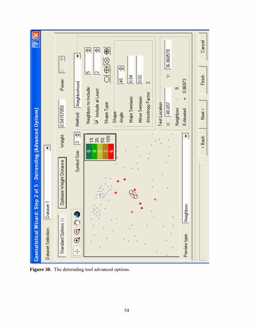
shows the “Advanced Options” parameters, available where parameters may be set to perform
more precise detrending.
52
Figure 28. Based on information gained from the ESDA process, the universal cokriging method is selected and the type of output surface to be produced is a map showing predicted values across the study area based on measured values from a limited number of sample locations.
53
Figure 29. The detrending tool standard options.
54
Figure 30. The detrending tool advanced options.
55
In modeling the semivariogram and covariance, parameters are selected by default by the
Geostatistical Wizard, each optimized according to the input dataset (Figure 31). These
parameters include the range, partial sill, nugget, lag size, and number of lags, which describe the
semivariogram model and may be entered manually. When viewing the semivariogram model,
the curve fitted to the plotted points levels out at a particular distance. The distance at which the
curve begins to flatten out is the range. Points within the range are autocorrelated, whereas
points beyond the range are not autocorrelated. In theory, the value of the semivariogram at zero
separation distance is zero. As a result of measurement errors, however, the semivariogram
value at infinitely small separation distance is usually greater than zero. This is referred to as the
nugget. The sill is defined as the value on the y-axis corresponding to the range on the x-axis.
The partial sill is then defined as the sill minus the nugget. Construction of the semivariogram
involves placing the data into bins of similar values. This is done to reduce the number of points
displayed in the semivariogram plot, making the necessary calculations manageable. The lag
size determines the size of the bins. Lag size must be chosen carefully, because small-scale
variation may be masked by a lag size that is too large, whereas a lag size that is too small may
overly smooth the results. Both the semivariogram and covariance clouds can be viewed. A
search direction may be defined if directional influences are suspected in the data.
The final selection to be made is a function to define the semivariogram and covariance.
Functions available include circular, spherical, tetraspherical, pentaspherical, exponential,
Gaussian, rational quadratic, hole effect, K-Bessel, J-Bessel, and stable. The
semivariogram/covariance model can be defined by one function, or a combination of up to three
functions. After examining the fit of the curves to the semivariogram and the resulting error
values, it was determined that the addition of the spherical and exponential functions produced
the lowest prediction errors.
The covariance of the dataset was also examined (Figure 32). In the covariance cloud,
the covariance is plotted as a function of distance, so data that are closer together should show
higher covariance.
56
Figure 31. Modeling the semivariogram/covariance.
57
Figure 32. Modeling the covariance.
58
Search neighborhoods may be defined for both datasets (Figure 33). Parameters to be
selected include the number and minimum number of neighbors used, shape type, and details
concerning the orientation, shape, and size of the search neighborhood. A preview of the sample
points and search neighborhood, and a preview of the output surface can be viewed. In the
preview of the search neighborhood, any point on the map may be selected to show which
sample points will be included in the calculation of the predicted value at that point. The x- and
y-coordinates, number of neighbors, and predicted value at a given location are displayed.
Cross-validation completes the model-fitting process. Multiple options are available for
viewing plots of predicted versus measured values (Figure 34), error versus measured values
(Figure 35), standardized error versus measured values (Figure 36), and a QQ plot of
standardized error versus normal values (Figure 37). A table consisting of the coordinates of
each measured sample point along with statistics associated with each point, including measured
and predicted values, error, standard error, standardized errors, and normal values, results. In
addition, measures of interpolation accuracy are provided in the form of statistics of the
prediction errors. These statistics are used to assess and compare the accuracy of one output
surface to another.
When cross-validation is complete, a summary of the method and selected parameters is
displayed (Figure 38). The resulting derivative map is shown in Figure 39. The new output
surface layer is added to the basemap. Summary information and a legend are shown in the
map’s table of contents. A prediction standard error surface can be produced showing spatially
the relative uncertainty in the predictions. A discussion of the results is provided in the
following chapter.
59
Figure 33. Definition of the search neighborhood for dataset 1. A unique search neighborhood may be defined for dataset 2.
60
Figure 34. Cross-validation involves the interpretation of prediction error statistics. Shown is the predicted versus measured values plot.
61
Figure 35. Plot of error versus measured value. The more accurate the predictions, the closer the points should plot to the line.
62
Figure 36. Plot of standardized error versus measured value.
63
Figure 37. Plot of standardized error versus normal value QQ.
64
Figure 38. Prior to generation of the output surface, the Geostatistical Wizard displays a summary of the parameters selected for interpolation.
65
Figure 39. The output surface showing distribution of DSP values. See Appendix B for interpolations of the DSP and V30 attributes using other techniques available in ArcMap 9.1.
66
5.0 Output Surfaces and Prediction Error Statistics
5.1 Prediction accuracy
Measures of prediction accuracy calculated by Geostatistical Analyst are provided during
cross-validation and include the mean, root-mean-square, average standard error, mean
standardized, and the root-mean-square standardized error. The mean and root-mean-square are
available for both geostatistical (kriging) and deterministic (e.g., splines) interpolation methods.
The average standard error, mean standardized, and root-mean-square standardized statistics,
which provide measures of uncertainty in the predictions (i.e., how good are the predictions) are
available only for the geostatistical methods, however.
Parameters may be selected and changed to achieve optimal prediction error statistics.
Once the process has been completed, the prediction errors associated with each method can be
compared, as well as graphs of the predicted, error, standardized error, and QQ plots from each
method (Figure 40).
5.2 Mean Dynamic Site Period (DSP)
5.2.1 Prediction Map
Universal cokriging, using depth-to-bedrock values as a correlating variable, was used to
produce the DSP prediction map. The resulting prediction error values suggest this method
produced the most accurate results. If the predicted values are unbiased (centered on the true
values), the mean should be near zero. For this interpolation, the calculated mean was –
0.005278. The root-mean-square error (RMS) measures how close the predicted values are to
the measured values, and the RMS should be as small as possible (the closer to zero the better).
The RMS was 0.2298.
The remaining measurements detail the validity of the results, describing the uncertainty
in the predictions. Average standard error (ASE) is a measure of the variability of the prediction
and should be close to the RMS value. Here, the ASE was 0.1989, a difference of 0.0309 from
the RMS. If the ASE is greater than the RMS
67
Figure 40. The cross validations from multiple output surfaces can be compared side-by-side.
68
the variability in prediction is overestimated, and if the ASE is less than the RMS, the prediction
variability is underestimated. The mean prediction error depends on the scale of the data, so the
mean standardized error is calculated by dividing the prediction errors by the prediction standard
errors. The mean standardized error should be as close to zero as possible. In this case, the
calculated value was –0.02963. Root-mean-square standardized error is another measure of
variability and is calculated by dividing each prediction error by its estimated prediction standard
error. These values should be similar, resulting in RMS standardized values close to 1 if the
prediction standard errors are valid. If the value is greater than 1, the prediction variability is
underestimated. Values less than 1 indicate overestimation of variability. The interpolation of
DSP using universal cokriging resulted in an RMS standardized value of 1.07.
Inspection of the DSP output surface allows conclusions to be drawn concerning the
geological and geophysical nature of the Jackson Purchase Region. First, trends in the
distribution of DSP values are clearly visible. Areas with mean dynamic site periods ranging
from 1.0 to 3.0 extend from north to south in parts of McCracken County (predominantly in the
central and western sections of the county), Ballard County (predominantly in the southeastern
half of the county), Carlisle County (in most areas except in the east), Hickman County
(covering the vast majority of the county), and Fulton County (in the northwestern and
northeastern sections of the visible study area). Parts of west-central, east-central, and
northeastern Graves County show DSP values above 1.0, as well as the northern half of Marshall
County and the eastern half of Calloway County.
Figure 41 shows the DSP output surface with bedrock depth distribution. The positive
correlation between the two variables is observed graphically where deeper bedrock depths align
with higher dynamic site periods.
Caution should be taken when examining areas of the map with few sample points (e.g.,
the northwestern, south-central, and eastern edges of the map, as well as the north-central and
south-central parts of Graves and McCracken Counties, respectively). Two additional areas,
central Hickman County and west-central Graves County, also contain few sample points. In
these areas, the scarcity of sample points results in less-reliable predictions, sometimes referred
to as “edge effects.”
69
Figure 41. Distribution of bedrock depths over DSP output surface. Higher dynamic site periods correlate with deeper sediments.
70
5.2.2 Prediction Standard Error Map
The prediction standard error map shows the distribution of prediction standard errors
calculated for every point on the output surface (Figure 42). Higher error values are represented
by darker colors, and lower error values by lighter colors. As expected, error values are highest
in areas with the fewest sample points, such as in north-central Graves County. In this area,
errors with values as high as about 0.3 are recorded, whereas in the vicinity of Paducah in
McCracken County, where many more sample points are located, providing better control on the
distribution of DSP values, error values of about 0.09 are common.
Using the prediction standard error map, areas can be identified where additional field
measurements may be necessary. Conversely, areas of high sampling density and, therefore high
confidence in the predicted values, can be identified. For example, if knowledge of the mean
dynamic site period for locations in north-central Graves County is needed, additional field
investigation to determine DSP should be conducted rather than relying completely on the values
predicted by Geostatistical Analyst.
71
Figure 42. The prediction standard error map derived from the DSP prediction map shows graphically the calculated uncertainty in the predictions. Light colors represent areas of low uncertainty, and dark colors represent high uncertainty as a result of lack of sample locations.
72
5.3 Weighted Shear-Wave Velocity of the Upper 30 m of Soil (V30)
The interpolation techniques used for the DSP output surfaces, other than cokriging, were
also used to interpolate V30 values over the same study area using data collected at the same
sample locations (Figure 43). Resulting accuracy statistics indicate that prediction of V30 values
over the study area was unsuccessful (Figure 44). The prediction error statistics were:
Mean: –0.1273
RMS: 79.7
Average standard error: 73.13
Mean standardized: –0.003095
RMS standardized: 1.078
The RMS error shows that there was a very large discrepancy in the predicted values
versus the actual measured values. For this reason, the output surface of interpolated V30 values
is not considered a true representation of the geophysical reality of the Jackson Purchase Region
and should not be used to infer relationships of V30 values from one location to another within
the study area. Figure 45 is a prediction standard error map derived from the V30 prediction map
showing areas of high uncertainty in areas with few sample locations.
The difficulty with interpolation of V30 arises as a result of the lateral variation in
stratigraphy in the Jackson Purchase. Thicknesses of individual soil layers and their s-wave
velocities are used for V30 calculation. The thickness of a layer determines how much weight is
given to its velocity, as shown in the equation V30 = 30/Σni=1(hi/vi) (BSSC, 1997). High variation
in stratigraphy, thicknesses of individual soil layers, and layer velocities over short distances
within the study area cause high interpolation prediction errors. In contrast, DSP values are
dependent only on the total thickness of the soil/sediment overburden and the weighted-average
velocity of all layers, parameters that are much more consistent over the entire study area than
thicknesses and velocities of individual layers. This accounts for the discrepancy in prediction
error statistics of DSP and V30 values.
73
Figure 43. The output surface showing distribution of V30 values.
74
Figure 44. Cross-validation summary statistics of prediction errors for V30 output surface.
75
Figure 45. Prediction standard error map derived from V30 output surface.
76
5.4 Deterministic Methods
In addition to the kriging methods, deterministic techniques were considered. Although
these methods, including inverse distance weighted (IDW), global and local polynomial, and
radial basis functions, including splines, produced surfaces with RMS values approximately
0.45, no means are available for assessment of uncertainty in the predictions. These methods are
ideal for fast interpolation and can provide output surfaces for use in general examination of
trends in a study area when no detailed uncertainty statistics are necessary.
The surface shown in Figure 46 was produced using a completely regularized spline. The
RMS error was 0.4412 with mean prediction error of –0.007481. Although the RMS error was
smaller using the universal cokriging method, the spline method still produced a relatively
accurate result. Though there are no associated measures of uncertainty, and prediction standard
error maps cannot be created from deterministic method output surfaces, the spline output
surface can be compared with the kriging surface to show the similarities between them.
Cokriging clearly produces a more detailed surface, but the spline surface shows agreement with
the major trends in DSP distribution across the study area.
OBJECTID THICK_SED_ SITE_CLASS Shape 1 17.5 SC-III Point 2 18.5 SC-III Point 3 20.6 SC-III Point 4 8.8 SC-III Point 5 13.7 SC-IV Point 6 9.5 SC-III Point 7 12.6 SC-IV Point 8 16.9 SC-III Point 9 13.7 SC-III Point
10 20.9 SC-III Point 11 22.2 SC-III Point 12 17.2 SC-III Point 13 16.8 SC-IV Point 14 26.2 SC-III Point 15 27.4 SC-IV Point 16 25 SC-III Point 17 23.1 SC-III Point 18 23.8 SC-III Point 19 29 SC-III Point 20 19.6 SC-IV Point
85
21 11.5 SC-IV Point 22 44.8 SC-III Point 23 20 SC-IV Point 24 13.9 SC-IV Point 25 30.8 SC-III Point 26 28.6 SC-III Point
Higgins–Henderson, KY, sites.
86
OBJECTID SITE LAT LONG_ V30 ARRAY OFFSET_1__ 1 701 35.883 -89.949 671 B 20 2 702 35.931 -89.98 663 B 400 3 703 35.887 -90.029 686 B 20 4 704 35.985 -90.042 674 B 400 5 705 35.857 -89.979 647 B 400 6 706 35.796 -89.942 657 B 400 7 707 35.785 -90.036 631 B 400 8 708 35.858 -90.074 679 B 400 9 709 35.956 -90.165 628 B 400
10 710 35.911 -90.225 638 B 400 11 711 35.836 -90.176 658 B 400 12 712 35.76 -90.149 698 B 400 13 713 35.895 -89.86 623 B 400 14 714 35.965 -89.819 592 B 400 15 715 35.859 -89.829 707 B 400 16 716 35.792 -89.846 658 B 400 17 717 35.917 -90.917 684 B 400 18 718 35.982 -90.361 701 B 400 19 719 35.847 -90.357 710 B 400 20 720 35.861 -90.404 632 B 400 21 721 35.797 -90.429 676 B 400 22 722 35.907 -90.469 696 B 400 23 723 35.985 -90.487 785 B 400 24 724 35.977 -90.533 859 B 400 25 725 35.903 -90.55 685 B 400 26 726 35.912 -90.711 675 B 400 27 727 35.989 -90.709 1503 B 400 28 728 35.981 -90.8 713 B 400 29 729 35.924 -90.854 751 B 400 30 730 35.84 -90.856 833 B 400 31 731 35.767 -90.786 950 B 400 32 732 35.777 -90.763 756 B 400 33 733 35.767 -90.553 0 B 400 34 734 35.672 -89.964 700 C 20 35 735 35.695 -90.035 595 C 20 36 736 35.726 -90.157 603 C 20 37 737 35.684 -90.22 664 C 20 38 738 35.722 -90.344 698 C 20 39 739 35.659 -90.322 665 C 20 40 740 35.57 -90.341 713 C 20 41 741 35.145 -90.103 626 B 20 42 742 35.193 -90.23 596 B 20 43 743 35.081 -90.222 602 B 20 44 744 35.693 -90.486 743 B 0 45 745 35.706 -90.554 688 B 0 46 746 35.671 -90.606 697 B 0 47 747 35.657 -90.648 782 B 0
87
48 748 35.655 -90.713 845 B 0 49 749 35.695 -90.833 0 B 0 50 750 35.565 -90.797 840 B 0 51 751 35.402 -90.785 923 B 0 52 752 35.325 -90.812 919 B 0 53 753 35.167 -90.847 883 B 0 54 754 35.067 -90.843 844 B 0 55 755 35.581 -90.972 586 C 20 56 756 35.53 -90.087 612 C 20 57 757 35.575 -90.2 660 C 20 58 758 35.567 -90.384 633 C 20 59 759 35.569 -90.558 695 C 20 60 760 35.583 -90.732 928 C 20 61 761 35.555 -90.948 923 C 20 62 762 35.55 -91.057 751 C 20 63 763 35.518 -91.201 682 C 20 64 764 35.446 -91.199 614 C 20 65 765 35.327 -91.193 761 C 20 66 766 35.582 -91.557 3899 C 20 67 767 35.57 -91.612 1176 C 20 68 768 35.599 -91.324 737 C 20 69 769 35.714 -91.202 725 C 20 70 770 35.815 -91.169 782 C 20 71 771 35.145 -90.686 652 C 20 72 772 35.204 -90.56 684 C 20 73 773 35.551 -90.554 740 C 20 74 774 35.287 -90.706 1152 C 20 75 775 35.354 -90.571 726 C 20 76 776 35.268 -90.447 753 C 20 77 777 35.34 -90.321 649 C 20 78 778 35.264 -90.321 696 C 20 79 779 35.266 -90.202 614 C 20 80 788 35.196 -90.91 895 B 0 81 789 35.193 -91.087 821 B 0 82 790 35.936 -90.663 752 B 0 83 791 35.471 -90.465 720 B 0 84 792 35.451 -90.52 767 B 0 85 793 35.397 -90.417 780 B 0 86 794 35.463 -90.359 774 B 0 87 795 35.453 -90.274 720 B 0 88 796 35.435 -90.208 644 B 0
OBJECTID OFFSET_2__ OFFSET_3__ OFFSET_4__ ELE___FT_ Shape 1 400 20 400 245 Point 2 20 20 400 248 Point 3 400 20 400 240 Point 4 20 20 400 240 Point 5 20 20 400 239 Point 6 20 20 400 240 Point
88
7 20 20 400 232 Point 8 20 20 400 239 Point 9 20 20 400 239 Point
10 20 20 400 237 Point 11 20 400 20 231 Point 12 20 400 20 231 Point 13 20 20 400 250 Point 14 20 20 400 256 Point 15 20 400 20 254 Point 16 20 400 20 248 Point 17 20 400 20 236 Point 18 400 20 20 238 Point 19 20 400 20 233 Point 20 20 400 20 229 Point 21 400 20 20 224 Point 22 400 20 20 233 Point 23 400 20 20 247 Point 24 20 400 20 280 Point 25 20 400 20 248 Point 26 20 400 20 311 Point 27 400 20 20 373 Point 28 400 20 20 253 Point 29 400 20 20 248 Point 30 400 20 20 259 Point 31 400 20 20 255 Point 32 400 20 20 237 Point 33 400 20 0 226 Point 34 0 20 0 244 Point 35 0 20 0 235 Point 36 0 20 0 232 Point 37 0 20 0 228 Point 38 0 20 0 223 Point 39 0 20 0 222 Point 40 0 20 0 218 Point 41 20 400 0 210 Point 42 400 20 400 220 Point 43 20 400 0 214 Point 44 240 0 240 221 Point 45 240 0 240 223 Point 46 240 0 240 223 Point 47 240 0 240 225 Point 48 230 0 240 248 Point 49 240 0 240 247 Point 50 240 0 240 245 Point 51 240 0 240 255 Point 52 240 0 240 244 Point 53 240 0 240 224 Point 54 240 0 240 218 Point
89
55 0 20 0 236 Point 56 0 20 0 225 Point 57 0 20 0 224 Point 58 0 20 0 216 Point 59 0 20 0 214 Point 60 0 20 0 257 Point 61 0 20 0 230 Point 62 0 20 0 230 Point 63 0 20 0 220 Point 64 0 20 0 225 Point 65 0 20 0 208 Point 66 0 20 0 590 Point 67 0 20 0 220 Point 68 0 20 0 222 Point 69 0 20 0 242 Point 70 0 20 0 247 Point 71 0 20 0 220 Point 72 0 20 0 207 Point 73 0 20 0 217 Point 74 0 20 0 255 Point 75 0 20 0 213 Point 76 0 20 0 213 Point 77 0 20 0 216 Point 78 0 20 0 224 Point 79 0 20 0 220 Point 80 240 0 240 219 Point 81 240 0 240 218 Point 82 240 0 240 224 Point 83 240 0 240 213 Point 84 240 0 240 212 Point 85 240 0 240 220 Point 86 240 0 240 220 Point 87 240 0 240 219 Point 88 240 0 240 230 Point
OBJECTID DATE_ TOPO ARRAY OFFSET_1 OFFSET_2 1 21-May-96 Wyatt A 20 220 2 21-May-96 Wyatt A 20 220 3 21-May-96 Charleston A 20 200 4 21-May-96 Charleston A 20 200 5 21-May-96 Bertrand A 20 200 6 21-May-96 Bertrand A 20 200 7 21-May-96 Sikeston N A 20 200 8 21-May-96 Sikeston N A 20 200 9 22-May-96 Morley A 20 200
10 22-May-96 Morley A 20 200 11 22-May-96 Thebes A 20 200 12 27-Jun-96 Vanduser A 20 200 13 27-Jun-96 Vanduser A 20 200 14 28-Jun-96 Oran A 20 200 15 28-Jun-96 Oran A 20 200 16 28-Jun-96 Chaffee A 20 200 17 28-Jun-96 Chaffee A 20 200 18 28-Jun-96 White Water A 20 200 19 28-Jun-96 Bell City A 20 200 20 28-Jun-96 Clines Island A 20 200 21 28-Jun-96 Clines Island A 20 200 22 28-Jun-96 Bloomfield A 20 200 23 29-Jun-96 Anniston A 20 200 24 29-Jun-96 Wickliffe SW A 20 200 25 16-Jul-96 New Madrid A 20 200 26 16-Jul-96 Kewanee A 20 200 27 16-Jul-96 Kewanee A 20 240 28 16-Jul-96 Sikeston S A 20 200 29 16-Jul-96 Sikeston S A 20 200 30 17-Jul-96 Point A 20 200
93
Pleasant
31 17-Jul-96 Point
Pleasant A 20 200 32 31-Jul-96 Morehouse A 20 200 33 31-Jul-96 Morehouse A 20 200 34 31-Jul-96 Charter Oak A 20 200 35 31-Jul-96 Charter Oak A 20 200 36 31-Jul-96 Hills Store A 20 200 37 31-Jul-96 Hills Store A 20 200 38 31-Jul-96 Bernie A 20 200 39 31-Jul-96 Dexter A 20 200 40 31-Jul-96 Essex A 20 200 41 01-Aug-96 East Prairie A 20 200 42 01-Aug-96 East Prairie A 20 200 43 01-Aug-96 Wyatt A 20 200 44 05-Aug-96 Caruthersville A 20 200 45 05-Aug-96 Caruthersville A 20 200 46 06-Aug-96 Catron A 20 200 47 06-Aug-96 Catron A 20 200 48 06-Aug-96 Parma A 20 200 49 06-Aug-96 Parma A 20 200 50 06-Aug-96 Malden A 20 200 51 06-Aug-96 Malden A 20 200 52 06-Aug-96 Valley Ridge A 20 200 53 06-Aug-96 Campbell A 20 200 54 06-Aug-96 Campbell A 20 200 55 06-Aug-96 Gideon A 20 200 56 07-Aug-96 Portageville A 20 200 57 07-Aug-96 Portageville A 20 200 58 07-Aug-96 Boekerton A 20 200 59 07-Aug-96 Boekerton A 20 200 60 07-Aug-96 Gideon A 20 200 61 07-Aug-96 Kenneth N A 20 200 62 07-Aug-96 Kenneth N A 20 200 63 07-Aug-96 Bragg City A 20 200 64 07-Aug-96 Bragg City A 20 200 65 07-Aug-96 Wardell A 20 200 66 08-Aug-96 Hayti Heights A 20 200 67 08-Aug-96 Deering A 20 200 68 08-Aug-96 Hayti Heights A 20 200
69 12-Aug-96 Cottonwood
Point A 20 200 70 12-Aug-96 Steele A 20 200 71 12-Aug-96 Steele A 20 200 72 12-Aug-96 Denton A 20 200
94
73 12-Aug-96 Denton A 20 200 74 12-Aug-96 Deering A 20 200 75 13-Aug-96 Kennett S A 20 200 76 13-Aug-96 Kennett S A 20 200 77 13-Aug-96 Senath A 20 200 78 13-Aug-96 Arbyrd A 20 200 79 13-Aug-96 Cardwell A 20 200 80 13-Aug-96 Arbyrd A 20 200 81 13-Aug-96 Homersville A 20 200 82 13-Aug-96 Homersville A 20 200 83 13-Aug-96 Stanley A 20 200 84 13-Aug-96 Wardell A 20 200
85 14-Aug-96 Hubbard
Lake A 20 200
86 14-Aug-96 Henderson
Mound A 20 200
87 14-Aug-96 Henderson
Mound A 20 200 88 14-Aug-96 Bayouville A 20 200 89 26-Aug-96 New Madrid A 20 200 90 26-Aug-96 Scott City A 20 200 91 26-Aug-96 Scott City A 20 200 92 26-Aug-96 Advance A 20 200 93 27-Aug-96 Dudley A 20 200 94 27-Aug-96 Powe A 20 200 95 27-Aug-96 Valley Ridge A 20 200 96 27-Aug-96 Kennett S A 20 200 97 26-Aug-96 Wickliffe SW A 20 200 98 26-Aug-96 Anniston A 20 200 99 26-Aug-96 Wolf Island A 20 200 100 02-Jul-98 Wyatt A 20 200
OBJECTID OFFSET_3 OFFSET_4 OFFSET_5 Shape 1 420 Point 2 420 620 820 Point 3 400 600 800 Point 4 400 600 800 Point 5 400 600 800 Point 6 400 600 800 Point 7 400 600 800 Point 8 400 600 800 Point 9 400 600 800 Point
10 400 600 800 Point 11 400 600 800 Point 12 400 600 800 Point 13 400 600 800 Point
95
14 400 600 Point 15 400 600 Point 16 400 600 Point 17 400 600 Point 18 400 600 Point 19 400 600 Point 20 400 600 Point 21 400 600 Point 22 400 Point 23 400 600 Point 24 400 600 800 Point 25 400 600 800 Point 26 400 600 800 Point 27 460 680 Point 28 400 600 800 Point 29 400 600 800 Point 30 400 600 800 Point 31 400 600 800 Point 32 400 600 800 Point 33 400 600 800 Point 34 400 600 800 Point 35 400 600 800 Point 36 400 600 800 Point 37 400 600 800 Point 38 400 600 800 Point 39 400 600 800 Point 40 400 600 800 Point 41 400 600 800 Point 42 400 600 800 Point 43 400 600 800 Point 44 400 600 800 Point 45 400 600 800 Point 46 400 600 800 Point 47 400 600 800 Point 48 400 600 800 Point 49 400 600 800 Point 50 400 600 800 Point 51 400 600 800 Point 52 400 600 800 Point 53 400 600 800 Point 54 400 600 800 Point 55 400 600 800 Point 56 400 600 800 Point 57 400 600 800 Point
96
58 400 600 800 Point 59 400 600 800 Point 60 400 600 800 Point 61 400 600 800 Point 62 400 600 800 Point 63 400 600 800 Point 64 400 600 800 Point 65 400 600 800 Point 66 400 600 800 Point 67 400 600 800 Point 68 400 600 800 Point 69 400 600 800 Point 70 400 600 800 Point 71 400 600 800 Point 72 400 600 800 Point 73 400 600 800 Point 74 400 600 800 Point 75 400 600 800 Point 76 400 600 800 Point 77 400 600 800 Point 78 400 600 800 Point 79 400 600 800 Point 80 400 600 800 Point 81 400 600 800 Point 82 400 600 800 Point 83 400 600 800 Point 84 400 600 800 Point 85 400 600 800 Point 86 400 600 800 Point 87 400 600 800 Point 88 400 600 800 Point 89 400 600 800 Point 90 400 600 800 Point 91 400 600 800 Point 92 400 600 800 Point 93 400 600 Point 94 400 600 800 Point 95 400 600 800 Point 96 400 600 800 Point 97 400 600 800 Point 98 400 600 800 Point 99 400 600 800 Point 100 400 600 800 Point
OBJECTID ELEVATION_ ARRAY OFFSET_1 OFFSET_21 325 A 20 2002 369 A 20 200
99
3 275 A 20 2004 285 A 20 2005 376 C 0 06 360 B 20 4007 329 B 20 4008 345 C 0 09 350 C 0 0
10 340 C 0 011 435 C 0 20012 380 C 0 013 410 C 0 014 550 C 0 015 425 C 0 016 480 C 0 40017 380 C 0 018 400 C 0 019 299 C 400 020 290 C 0 40021 310 C 0 022 330 C 0 023 300 C 0 024 300 C 0 025 323 C 0 026 300 C 0 027 350 C 0 028 340 C 0 40029 370 C 0 030 450 C 0 031 510 C 0 032 387 C 0 033 396 C 0 034 430 C 0 035 480 C 0 036 465 C 0 037 510 C 0 038 440 C 0 039 355 C 0 041 405 C 0 042 385 C 0 043 395 C 0 044 310 C 0 045 385 C 0 046 460 C 0 047 485 C 0 0
100
48 415 C 0 049 510 C 0 050 460 C 4 051 540 C 4 052 300 B 20 40053 300 B 20 40054 280 B 20 32055 283 B 20 32056 280 B 20 32057 270 B 20 32058 272 B 20 32059 300 B 20 32060 270 C 20 061 295 C 20 062 326 C 20 063 353 C 20 064 372 C 0 2065 340 C 20 066 390 C 20 067 480 C 20 068 500 C 20 2069 280 B 0 9670 410 B 0 40071 340 B 0 40072 320 B 0 40073 370 B 0 40074 350 B 0 40075 300 B 0 40076 280 B 0 40077 270 B 0 40078 300 B 0 40079 350 B 0 40080 250 B 0 40081 290 B 0 40082 500 20 140
Ordinary Kriging (V30) Mean: 0.6137 Root-Mean-Square: 79.55 Average Standard Error: 68.96 Mean Standardized: 0.008499 Root-Mean-Square Standardized: 1.133
136
Simple Kriging (V30) Mean: 1.155 Root-Mean-Square: 80.36 Average Standard Error: 64.16 Mean Standardized: 0.01027 Root-Mean-Square Standardized: 1.21
137
Universal Kriging (V30) Mean: 0.09248 Root-Mean-Square: 79.32 Average Standard Error: 68.29 Mean Standardized: 0.001597 Root-Mean-Square Standardized: 1.143
138
References
Al-Yazdi, Ali Ahmed. 1994. Paleozoic bedrock depth investigation in the Jackson Purchase Region of western Kentucky using the P-wave seismic reflection technique for the purpose of regional 1-D site effects estimation. University of Kentucky, Thesis.
Arlinghaus, Sandra L. 1996. Practical Handbook of Spatial Statistics. CRC Press, Boca Raton,
FL. BSSC. 1997. NEHRP Recommended Provisions for Seismic Regulations for New Buildings,
Part 1 — Provisions. 1997 Edition, Building Seismic Safety Council, Washington, D.C.: 337 pp.
Carr, James R. 1995. Numerical Analysis for the Geological Sciences. Upper Saddle River,
New Jersey: Prentice-Hall, Inc. Carver, Steve. 1997. Innovations in GIS 5. Taylor and Francis, Inc. Bristol, Pa. Christakos, G., Bogaert, P., and Serre, M. 2001. Temporal GIS: Advanced Functions for Field-
Based Applications. Berlin: Springer-Verlag. Cressie, Noel A. 1991. Statistics for Spatial Data. New York: John Wiley and Sons. Davis, John C. 1986. Statistics and Data Analysis in Geology (2nd Edition). New York: John
Wiley and Sons. Deutsch, Clayton V., and Journel, Andre G. 1998. GSLIB: Geostatistical software library and
user’s guide (2nd Edition). New York: Oxford University Press, Inc. Dowdy, Therese C. 1998. Application of a GIS to a hydrogeologic investigation of the Inner
Bluegrass karst region in Scott County, Kentucky. University of Kentucky, Thesis. ESRI Virtual Campus Web Course. 2004. Creating, Editing, and Managing Geodatabases for
ArcGIS 8.3. campus.esri.com/index.cfm. (Accessed March, 2005). ESRI. 2006. www.esri.com. Accessed February, 2006. Foresman, Timothy W. 1998. The History of Geographic Information Systems. Upper Saddle
River, N.J.: Prentice Hall, Inc. Goovaerts, Pierre. 1997. Geostatistics for Natural Resources Evaluation. New York: Oxford
University Press, Inc.. Haining, Robert. 1990. Spatial data analysis in the social and environmental sciences.
Cambridge [England]: Cambridge University Press, 409 pp.
139
Harris, James B. 1992. Site amplification of seismic ground motions in the Paducah, Kentucky, area. University of Kentucky, Thesis.
Hernandez, Michael J. 1997. Database Design for Mere Mortals: A Hands-On Guide to
Relational Database Design. Reading, Mass.: Addison Wesley Longman, Inc. Higgins, Brian A. 1997. Site amplification of earthquake ground motions in unconsolidated
sediments in Henderson, Kentucky. University of Kentucky, Thesis. Hoffer, Jeffrey A., Prescott, Mary B., and McFadden, Fred R. 2005. Modern Database
Management (7th Edition). Upper Saddle River, N.J.: Pearson Education, Inc. Hohn, Michael E. 1999. Geostatistics and Petroleum Geology. Dordrecht, The Netherlands:
Kluwer Academic Publishers. Isaaks, Edward H., and Srivastava, R. Mohan. 1989. An Introduction to Applied Geostatistics.
New York: Oxford University Press. Johnston, A.C., and Nava, S.J. 1985. Recurrence rates and probability estimates for the New
Madrid Seismic Zone. Journal of Geophysical Research, 90, 6737–6753. Journel, Andre G. 1989. Fundamentals of Geostatistics in Five Lessons. Washington, D.C.:
American Geophysical Union. Kanevski, Mikhail, and Maignan, Michel. 2004. Analysis and Modelling of Spatial
Environmental Data. New York: EPFL Press. Kim, Dong-Soo, Chung, Choong-Ki, Sun, Chang-Guk, Bang, Eun-Seok. 2002. Site assessment
and evaluation of spatial earthquake ground motion of Kyeongju. Soil Dynamics and Earthquake Engineering 22, 371–387.
Laslett, G.M. 1994. Kriging and splines: An empirical comparison of their predictive
performance in some applications. Journal of the American Statistical Association, 89 (426), 391–409.
Lin, T. 2003. Local soil-induced amplification of strong ground motion in Maysville, Kentucky.
University of Kentucky, Thesis. Middleton, Gerard V. 2000. Data analysis in the earth sciences using MATLAB. Upper Saddle
River, N.J.: Prentice Hall. Nuttli, O.W. 1973. The Mississippi Valley earthquakes of 1811 and 1812, intensities, ground
motion, and magnitude. Seismological Society of America Bulletin, 63, 227–248.
140
Olive, W.W. 1972. Geology of the Jackson Purchase Region, Kentucky: Roadlog for the Geological Society of Kentucky field excursion: Kentucky Geological Survey, Ser. 10, 11 p.
O’Sullivan, David, and Unwin, David J. 2003. Geographic Information Analysis. Hoboken,
NJ.: John Wiley and Sons. Ott, Thomas, and Swiaczny, Frank. 2001. Time-Integrative Geographic Information Systems.
Berlin: Springer-Verlag. Petry, Frederick E., Robinson, Vincent B., and Cobb, Maria A. 2005. Fuzzy Modeling with
Spatial Information for Geographic Problems. Berlin: Springer-Verlag. Riccardi, Greg. 2001. Principles of Database Systems with Internet and Java Applications.
Boston: Addison Wesley Publishing Company. Royle, A., Clark, Isobel, Brooker, P.I., Parker, H., Journel, A., Rendu, J.M., Sandefur, R., and
Mousset-Jones, Pierre. 1980. Geostatistics. New York: McGraw-Hill, Inc. Rutledge, Alex. 2004. High resolution geophysical investigation of late quaternary deformation
in the lower Wabash Valley Fault System. Thesis. University of Kentucky. Schabenberger, Oliver, and Gotway, Carol A. 2005. Statistical Methods for Spatial Data
Analysis. Boca Raton, Fla.: Chapman and Hall/CRC, 488 p..
Schwalb, H. R., 1969, Paleozoic geology of the Jackson Purchase Region, Kentucky, with reference to petroleum possibilities: Kentucky Geological Survey, ser. 10, Report of Investigations 10, 40 p.
Shi, Wenzhong, Fisher, Peter F., and Goodchild, Michael F. 2002. Spatial Data Quality.
London: Taylor and Francis. Street, R. 1982. A contribution to the documentation of the 1811–1812 Mississippi Valley
earthquake sequence. Earthquake Notes, 53 (2), 39–52. Street, R. 1996. Dynamic site periods in the northern Mississippi Embayment area of western
Kentucky and southeastern Missouri. Contract report to U.S. Geological Survey. Street, R., Woolery, E., Harik, I., Allen, D., and Sutterer, K. 1997. Dynamic Site Periods for the
Jackson Purchase Region of Western Kentucky. (KYSPR96-173). Research Report KTC-97-1. Kentucky Transportation Center.
141
Street, R., Woolery, E., Wang, Z., and Harik, I. 1997. Soil classifications for estimating site-dependent response spectra and seismic coefficients for building code provisions in western Kentucky. Engineering Geology, 46, p. 331–347.
Street, R., Woolery, E., Wang, Z., and Harris, J. 2001. NEHRP soil classifications for
estimating site-dependent seismic coefficients in the Upper Mississippi Embayment. Engineering Geology, 62, 123–135.
Street, R., Wiegand, J., Woolery, E. W., and Hart, P. 2005. Ground-motion parameters of the
southwestern Indiana earthquake of 18 June 2002 and the disparity between the observed and predicted values. Seismological Research Letters, 76 (4).
Wang, Z. 1993. Qs estimation for unconsolidated sediments and site amplification of strong
ground motion in western Kentucky. University of Kentucky, Thesis, 94 p. Wang, Z., Cordiviola, S., and Kiefer, J. 2004. Earthquake Hazard Assessment for Louisville
Metropolitan Area, Kentucky. Kentucky Geological Survey Final Report. USGS. Wheeler, R. 1997. Boundary separating the seismically active Reelfoot Rift from the sparsely
seismic Rough Creek Graben, Kentucky and Illinois. Seismological Research Letters, 68, 586–598.
Wood, Steve. 2000. Ground-response analysis of the near-surface sediments in the Memphis,
Tennessee, metropolitan area. University of Kentucky, Thesis. Woolery, Edward W., Schaefer, Jeffrey A., and Wang, Zhenming. 2003. Elevated lateral stress
in unlithified sediment, Midcontinent, United States—Geotechnical and geophysical indicators for a tectonic origin. Tectonophysics, 368, 139–153.
Zeiler, Michael. 1999. Modeling Our World: The ESRI Guide to Geodatabase Design.
Environmental Systems Research Institute. Zhang, Jingxiong, and Goodchild, Michael. 2002. Uncertainty in Geographical Information.
New York: Taylor and Francis, Inc.
142
VITA
-Born February 10, 1977, in Santa Maria, California. Education -University of Kentucky, Lexington, Kentucky, 2000 – 2004 Bachelor of Science – Geology Experience -Research Assistant, Kentucky Geological Survey, 2001 – 2006 -Kentucky Army National Guard, 1999 – 2004 -United States Army, 1996 – 1999 Honors and Activities -Presented thesis research poster at the Seismological Society of America sectional meeting, 2005 -Presented research findings at the Seismological Society of America sectional meeting, 2005 -Recipient of Graduate School Pirtle academic scholarship, 2005 and 2006 -Attended field camp as a student, Montana; 6-week structural geology mapping course, 2004