Shearing Flows in Liquid Crystal Models

By

Timothy Dorn

Submitted to the graduate degree program in the Department of Mathematicsand the Graduate Faculty of the University of Kansas in partial fulfillment of the

requirements for the degree of Doctor of Philosophy.

Doctor of Philosophy

Committee members

Dr Weishi Liu, Chairperson

Dr Myunghyun Oh

Dr Milena Stanislavova

Dr Erik Van Vleck

Dr JiCong Shi, Physics and Astronomy

Date defended: March 26, 2012

The Dissertation Committee for Timothy Dorn certifiesthat this is the approved version of the following dissertation:

Shearing Flows in Liquid Crystal Models

Dr Weishi Liu, Chairperson

Date approved: April 13, 2012

ii

Abstract

The liquid crystal phase is a phase of matter between the solid and liquid phase whose

flow is characterized by a velocity field and a director field which describes locally

the orientation of the liquid crystal. In this work we explore shearing flows in two

related continuum models of liquid crystals. The first is a phenomenological model

of frictional forces in a geological fault, which is motivated by the second model, the

Leslie-Ericksen continuum theory of liquid crystals.

iii

Acknowledgements

First, I would like to thank my wife, Terra, for all her support and encouragement

throughout my entire graduate career. Also, my daughter Adelaide whose arrival gave

me a second wind.

I would like to thank my advisor Weishi Liu. When I was stumped, he was always

there get me through and guide me in the right direction.

Finally, I would like to thank everyone in the KU mathematics department. Espe-

cially professors Erik Van Vleck and Milena Stanislavova for their many conversations.

iv

Contents

Abstract iii

Acknowledgements iv

1 Introduction 1

1.1 Liquid Crystals . . . . . . . . . . . . . . . . . . . . . . . . . . . . . . 1

1.2 Classic Continuum Models for Liquid Crystals . . . . . . . . . . . . . 2

1.3 A Simplified Phenomenological Model . . . . . . . . . . . . . . . . . . 12

2 Shearing Flows in a Liquid Crystal Model for Friction 14

2.1 The steady state . . . . . . . . . . . . . . . . . . . . . . . . . . . . . . 18

2.1.1 Existence and multiplicity . . . . . . . . . . . . . . . . . . . . 18

2.1.2 An example of multiple steady states . . . . . . . . . . . . . . 24

2.2 Stability for small shearing speeds . . . . . . . . . . . . . . . . . . . . 25

2.2.1 Linear stability . . . . . . . . . . . . . . . . . . . . . . . . . . 26

2.2.2 Nonlinear stability . . . . . . . . . . . . . . . . . . . . . . . . 28

2.3 Eigenvalues and bifurcations of steady-states . . . . . . . . . . . . . . 30

2.3.1 Linearization, eigenvalues, and the Evans function . . . . . . . 30

2.3.2 The Characterization of a zero eigenvalue . . . . . . . . . . . . 33

2.3.3 Bifurcation of the zero eigenvalue . . . . . . . . . . . . . . . . 38

v

2.4 Hysteresis: a numerical simulation of dynamic boundary conditions . . 53

3 Shearing Flows in the Leslie-Ericksen Continuum Theory of Nematic Liq-

uid Crystals 56

3.1 The steady state system . . . . . . . . . . . . . . . . . . . . . . . . . . 63

3.2 Phase plane configurations . . . . . . . . . . . . . . . . . . . . . . . . 64

3.3 Existence in the region containing 5CB . . . . . . . . . . . . . . . . . 69

3.3.1 The time map technique . . . . . . . . . . . . . . . . . . . . . 69

3.3.2 Existence of single twist solutions . . . . . . . . . . . . . . . . 72

3.4 Further Research . . . . . . . . . . . . . . . . . . . . . . . . . . . . . 76

Figures 78

Bibliography 80

vi

Chapter 1

Introduction

In this work we explore shearing flows of liquid crystals in the context of both the

Leslie-Ericksen continuum theory of nematic liquid crystals and a simplified phenomeno-

logical continuum model for nematic liquid crystals proposed to describe frictional

forces in geological faults. The phenomenological model is a simplification of the

Leslie-Ericksen continuum theory, but still captures the underlying dynamics.

1.1 Liquid Crystals

The liquid crystal phase is a phase of matter between the liquid and solid phases. They

have flow properties of liquids, but because the molecules possess a highly anisotropic

structure they also exhibit properties of solids. Because of these properties liquid crys-

tals are are used in many applications including LCD televisions, thermometers, and

optical imaging.

At the microscopic level liquid crystals look like small rods and at the macroscopic

level these rods align themselves into locally preferred orientations modeled by a vector

field, n, called the director field, Figure 1.1.

1

Nematic Liquid CrystalSolid Liquiddirector

Figure 1.1: Nematic liquid crystal phase and director unit vector describing the local orienta-tion.

The discovery of liquid crystals is attributed to Dr Friedrich Reinitzer in 1888, [9].

Many materials exhibit a liquid crystal phase as the the material is heated or cooled,

called thermotropic liquid crystals, or by changes in concentration in a solvent, called

lyotropic liquid crystals. The thermotropic liquid crystal is commonly classified into

three different types:

1. Nematic: The molecules align on average locally into a preferred orientation.

2. Cholesteric: The molecules align on average locally into a preferred orientation

and also longitudinally align into a preferred helical configuration.

3. Smectic: The molecules align on average locally into a preferred orientation and

also into layers within the bulk of the material.

1.2 Classic Continuum Models for Liquid Crystals

The first static continuum theory, i.e. in the absence of positional movement, for ne-

matic liquid crystals is due to Zocher, [48, 49], and Oseen, [35], in the 1930s and then

was refined by Frank, [19], in 1958 to include cholesteric liquid crystals. The idea

2

behind the static continuum theory is to construct an energy density functional

W (n,∇n) (1.1)

which measures the localized average change in energy due to a deformation from a

natural undeformed state. The director field is the realization of local averaging to de-

scribe the natural state in a nematic liquid crystal, Figure 1.1. For any natural alignment

of the liquid crystal, n∗, one prescribes that W (n∗,∇n∗) = 0.

Since the director field is used to describe the locally averaged direction of the liquid

crystal it is modeled by a unit vector field

|n|= 1, (1.2)

and because of the rod like structure one does not differentiate between the orientations

n and −n. This along with the usual mechanics assumptions of frame indifference

W (n,∇n) = W (Qn,Q∇nQT ) (1.3)

for any orthogonal matrix Q, allowed Frank to derive the following formula for W ,

commonly referred to as Frank’s free energy formula.

W = K0τ(n ·∇×n+ τ)+K1(∇ ·n)2 +K2(n ·∇×n+ τ)2 (1.4)

+K3|n×∇×n|2 +(K2 +K4)(tr(∇n)2− (∇ ·n)2)

The parameter τ is a measure of the longitudinal twist associated with a cholesteric

liquid crystals with τ = 0 corresponding to the nematic liquid crystal. The constants

3

K1,K2,K3 are called Frank’s constants and are a measure of the liquid crystal materials

tendency to splay, twist, or bend respectively.

The energy density functional is defined up to a constant representing the minimal

energy in the natural configuration of the liquid crystal material. By taking this constant

to be zero, it is typical to assume that the energy density functional W is positive

definite, i.e.

W (n,N)≥ 0 (1.5)

for all n ∈ S2 and N ∈L (n,R3) where

L (n,R3) = N ∈L (R3) : NT n = 0 (1.6)

The space L (N,R3) arises naturally from the restriction (1.2) since taking the deriva-

tive on both sides yields

(Dn)T n = 0.

In 1966, Ericksen derived the inequalities

2K1 ≥ K2 +K4, K2 ≥ |K4|, K3 ≥ 0 (1.7)

which are necessary and sufficient conditions for (1.5) to hold.

To go from local theory to global theory one defines the energy functional

E [n] =ˆ

DW (n,∇n)dV. (1.8)

on a domain D with a smooth boundary ∂D and prescribed Dirichlet

n∣∣∂D

= 0

4

or Neumann∂n∂ν

∣∣∣∣∂D

= 0

boundary conditions. For static configurations one looks to find minimizers of the

energy functional E [n]. Minimizers which are not smooth are of particular interest as

they present defects in the alignment of the liquid crystal, [10]. Another approach is to

derive a set of Euler-Lagrange equations. This variational approach is especially useful

in examining special types of static director configurations, [45, 10, 44].

The dynamic continuum theory of liquid crystals was developed in series of papers

by Ericksen, [18], and Leslie, [28, 27], which summarize the dynamic continuum the-

ory. This is done via the classical approach of averaging the motion of the particles

in the liquid crystal material and defining the motion by a velocity field, u(t,x). The

derivation is analogous to that of the Navier-Stokes equations, [12], and we now give a

brief overview of how this is done.

Consider at each point x in a domain Ω∈R3 the motion of the liquid crystal material

through that point given by the velocity field u(t,x). For a function h : R×R3→ R3,

we define the material time derivative of h by the formula

DDt

h(t,x) =∂h∂ t

+(u ·~∇)h.

The acceleration is of the liquid crystal material through the point x is given by

a(t,x) =DuDt

.

Following the classical approach one assumes that for every open subset Wt ⊂Ω, trav-

eling along with the flow, the following conservation laws are true:

5

(i) Conservation of Massddt

ˆΩ

ρ dx = 0 (1.9)

where ρ(t,x) is the density per unit volume.

(ii) Conservation of Linear Momentum

ddt

ˆWt

ρudV =

ˆWt

FdV +

ˆ∂Wt

tdS (1.10)

where F is the external body force and t is the stress tensor with components

ti = t jiν j where ν is the outward pointing unit normal.

(iii) Conservation of Angular Momentum

ddt

ˆWt

ρ(x×u)+ρ1(n× n)dV =

ˆWt

x×F+n×GdV +

ˆ∂Wt

x× t+n× sdS

(1.11)

where G is the external director body force, ρ1 is a material constant, and s is the

director stress tensor with components si = s jiν j.

(iv) Conservation of Energy

ddt

ˆWt

12

ρ|u|2 + 12

ρ1|n|+E dV =

ˆWt

f ·u+G · ndV +

ˆ∂Wt

t ·u+ s · ndS (1.12)

where E is the internal energy per unit volume. Note, the left hand side constitutes

the kinetic energy due to the positional movement of the material plus the kinetic

energy of the liquid crystal material due to a non-natural static configuration of

the director field.

By converting the surface integrals into volume integrals and enforcing that the

conservation laws should hold on any arbitrary subset of Ω one obtains the differential

6

form of the conservation laws. Yet, the the domain Wt is traveling along with the flow,

thus the need for the following lemma which is proved in [12].

Lemma 1. [Transport Theorem] Suppose that ϕ : R×Ω→ Ω is the flow associated

with the differential equation x′ = u(t,x). Then, for any function f ∈C1(R×Ω,Ω),

ddt

ˆWt

f (x, t)dV =

ˆWt

D fDt

(x, t)+ f (x, t)∇ ·u(x, t)dV

where Wt = ϕ(t,W0) and W0 ⊂∈Ω is open. Moreover, if the vector field the u is incom-

pressible, i.e. ∇ ·u = 0, then

ddt

ˆWt

f (x, t)dV =

ˆWt

D fDt

(x, t)dV

In [28], Leslie assumes that the liquid crystal material is incompressible since a

majority of applications enforce this constraint,

∇ ·u = 0. (1.13)

The differential forms for the conservation of mass and conservation of linear momen-

tum, using Lemma 1 are straightforward to compute and are given respectively by

ρ = 0, (1.14)

ρ vi = Fi + t ji. j. (1.15)

where˙= DDt and we are using the Einstein summation convention which states that one

should sum over all repeated indices.

7

The differential form of (1.11) is more delicate. We differentiate and after eliminat-

ing the conservation of linear momentum term, (1.15), which arises we have

ei jk(ρ1n jnk−n jGk−n jspk,p) = ei jk(tk j +n j,pspk). (1.16)

The left hand side of equation is a vector orthogonal to n and thus so is the right hand

side. There exists a vector g such that n×g is equal to the right hand side of equation

(1.16) and so

ei jkn jgk = ei jk(tk j +n j,pspk), (1.17)

where ei jk is the alternating symbol. But, note that equation (1.17) doesn’t completely

determine the vector g since for any γ ∈ R the vector g≡ g+ γn also satisfies equation

(1.16). Equating terms in (1.16) and (1.17) we arrive at the differential form of the

conservation of angular momentum

ρ1ni = Gi +gi + s ji, j, (1.18)

where g is determined only up to the addition of a constant multiple of the director n

and satisfies equation (1.17). Finally we derive from the conservation of energy, after

eliminating terms arising from (1.15) and (1.18),

E = t jiu j,i + s j,in j,i−gini. (1.19)

In order to derive the constitutive relations on the the stress tensor t and s as well as

the intrinsic body force g we define the Hemoltz free energy

H = E−TS , (1.20)

8

where T is the internal temperature, which we assume to be constant, and S is the

entropy per unit volume. By the second law of thermodynamics one has S ≥ 0 and

hence rearranging the terms in (1.20) and substituting from (1.19) gives the inequality

t jiu j,i + s j,in j,i−gini−H ≥ 0. (1.21)

The derivation of the constitutive relations is due to Leslie [28]. The stress tensor

t ji is separated into an static part, t0ji, and a dynamic part, td

ji,

t ji = t0ji + td

ji, (1.22)

with

t0ji =−pδ ji−

∂H

∂nk, jnk,i, (1.23)

and

tdji = µ1nknmdkmnin j +µ2n jNi +µ3niN j +µ4d ji +µ5n jnkdki +µ6ninkdk j, (1.24)

where

Ni = ni−wiknk,

2di j = vi, j + v j,i,

2wi j = vi. j− v j,i,

p is an indeterminate constant, and µi, i= 1 . . .6 are referred to as the Leslie coefficients

of viscosity. The intrinsic director body force is also decomposed in to an static part,

g0i , and a dynamic part, gd

i ,

gi = g0i +gd

i , (1.25)

9

with

g0i = γni−β jni, j−

∂H

∂ni, (1.26)

and

gdi = λ1Ni +λ2n jd ji, (1.27)

where γ and β j are indeterminate constants, and

λ1 = µ2−µ3, λ2 = µ5−µ6. (1.28)

Also,

s ji = β jni +∂H

∂ni, j. (1.29)

In this work we will be considering shearing flows for the nematic liquid crystal

state. Thus we summarize the conservation laws for the nematic liquid crystal:

ρ v = fi + ti j, j, (1.30)

ρ1n = Gi +gi + s ji, j, (1.31)

2F = K1(∇ ·n)2 +K2(n ·∇×n)2 +K3|n×∇×n|2, (1.32)

where t ji, s ji, and gi are defined in (1.22), (1.29), and (1.25) respectively and F is

derived from Frank’s formula (1.4)

Because of the complexity inherent in the full Leslie-Ericksen continuum theory of

liquid crystals only recently has global existence of weak solutions been shown, [32,

31]. There are also many other active areas of research including Poiseuille flows [7, 8],

liquid crystals with variable degrees of orientation [29, 30, 6], static configurations and

Fredericks transitions [7, 34].

10

The second portion of this work is devoted to one-dimensional shearing flows within

the context of the Leslie-Ericksen continuum theory of liquid crystals. Much work has

been done in the area of shearing flows of nematic liquid crystals , but there are three

main drawbacks to the current analysis.

The first is a lack of analytic results concerning the multiplicity and stability of

steady state solutions. Using numerical methods McIntosh et. al., [33], were able

to show that only two types of solutions may be stable, which was a reduction to the

number of stable candidates proposed by Currie and MacSithigh, [15].

The second is a common set of simplifying assumptions made on intrinsic parame-

ters. More specifically the constant approximation

K1 = K2 = K3 (1.33)

of the Frank elasticity constants. As we will see, the constant approximation (1.33)

retards the possibility of multiplicity of solutions in a one-dimensional shearing flow.

The third is a reduction in complexity made by assuming the velocity field is con-

stant, [5]. While this is fine if one is concerned with this specific class of flows, we do

not make this assumption in the following work and thus present more general results.

In the one-dimensional shearing flow regime we consider, the liquid crystal is con-

fined between two parallel plates and a flow is induced via a shearing force applied to

the upper plate. In our work we first transform the steady state equations into a Hamil-

tonian system and proceed to construct the Hamiltonian. We then give a complete

description of the phase planes with respect to the parameter space

Λ = (λ1,λ2) ∈ R2, (1.34)

11

where λ1,λ2 are defined through the Leslie coefficients of visocity in (1.28).

Focusing in on a particularly relevant region, in that it contains many of the com-

monly referenced liquid crystal materials including Isopentyl-cyanobiphenyl (5CB), we

prove an existence result concerning steady state solutions subject to strong anchoring

boundary conditions via time map arguments.

1.3 A Simplified Phenomenological Model

In their paper, Cheng et. al. [11], the authors consider a nematic liquid crystal fluid

layer in between two parallel blocks to model frictional sliding in a geological fault.

The continuum model proposed to describe this situation is

ut +(u ·∇)u = div(v(r)∇u)− 1ρ

∇p, in Ω (1.35)

rt +∇r ·u−∇u · r = δ∆r, in Ω (1.36)

where u is the velocity of the fluid, r is the director field, ρ is the density, v(r) is the

kinematic viscosity, p is the pressure, δ is a relaxation parameter, and Ω denotes the

region bounded by the two solid blocks. The kinematic viscosity v(r) is assumed to

depend on the director field r via the model

v(r) = α(θ)v1 +(1−α(θ))v0

for some decreasing function α and 0 < v0 < v1, where

cosθ =|u× r||u||r|

.

12

The function α(θ) determines the type of frictions modeled. In [11], the authors in-

troduced the above model (2.1) and (2.2), and used numerical simulations to examine

the behavior of solutions that allow them to compare with the empirical rate-and-state

friction law. In our work we consider a more general form of the kinematic viscosity.

In order to understand the behavior in a geological fault, the authors consider a

reduction to a one-dimensional shearing flow between two parallel plates. The shearing

flow is assumed to be induced by a shearing velocity on the upper plate while the lower

plate is held fixed. Furthermore the director is subject to a strong anchoring boundary

condition, i.e. it is held in the same fixed direction on the upper and lower plate.

To begin, we completely describe the existence and multiplicity of the steady states.

We are able to do so by exploiting the inherent Hamiltonian structure of the steady state

equations. In the case that multiple steady-state solutions exist, it is natural to further

ask which solutions are linearly (spectrally) stable. Stable solutions are ones which

persist under small perturbation and hence are more physically realistic. We approach

the question of spectral stability in two ways: energy methods and the Evans function

[25, 24].

For small values shearing velocities we are able to show that the spectrum of the

linearized operator lies in the left half complex plane, i.e. the steady state solution

with small shearing velocity is spectrally stable. We are actually able to take this one

step further and show that in fact for small shearing speeds the steady state solution is

nonlinearly stable. Next we construct an Evans type function and show that zero is an

eigenvalue of the linearized operator precisely when there is a bifurcation of the steady

states.

Finally our spectral stability results suggest the possibility of an interesting hystere-

sis mechanism being present in this system. We use numerics to explore this subject.

For a shorter technical presentation of this work reference [11].

13

Chapter 2

Shearing Flows in a Liquid Crystal Model for Friction

In this section we explore a liquid-crystal type model which specifically attempts to

address the issue of frictional forces in geological fault flows. Recall, the nematic liquid

crystal continuum model proposed by C. H. A Cheng et. al., [11] which considers a

fluid layer composed of nematic liquid crystal confined between two solid blocks:

ut +(u ·∇)u = div(v(r)∇u)− 1ρ

∇p, in Ω (2.1)

rt +∇r ·u−∇u · r = δ∆r, in Ω (2.2)

where u is the velocity of the fluid, r is the director field, ρ is the density, v(r) is the

kinematic viscosity, p is the pressure, δ is a relaxation parameter, and Ω denotes the

region bounded by the two solid blocks.

To model the behavior of a fault the domain is taken to be Ω = (−∞,∞)× (0,L),

an infinite channel with width L, with coordinates (x,y) and is is assumed that there is

no external pressure, i.e. p ≡ 0. Let u = (u1(x,y),u2(x,y)) and r = (r1(x,y),r2(x,y))

denote the velocity and director fields respectively. Under further simplifications, see

14

[11], these fields are assumed to take the form

u1(x,y) = u(y), u2 = 0; r1(x,y) = r(y), r2 = 1. (2.3)

A shearing flow is then induced by an imposed shearing velocity on the upper block,

u, see Figure 2.1.

(u(y),0) (r(y),1)

(u,0)

Figure 2.1: Diagram of the shearing flow in an infinite channel

Under these assumptions and with v(r) = v(r), one obtains a one-dimensional ver-

sion of the model:

ut = (v(r)uy)y, rt = δ ryy +uy, for y ∈ (0,1), (2.4)

with the boundary conditions

u(0, t) = 0, u(1, t) = u; r(0, t) = r(1, t) = 0. (2.5)

In this shearing flow, the kinematic viscosity v(r) depends only on the director field r

via the model

v(r) = α(θ)v1 +(1−α(θ))v0

15

for some decreasing function α with α(0) = 1 and α(π/2) = 0 and 0 < v0 < v1, where

θ is the angle of r from the vertical.

In our analysis we consider a general v(r) and assume

0 < v0 ≤ v(r)≤ v1, v′(r)≤ 0 and

either v′(r) = 0 for large r or limr→∞

(v′(r))2

v′′(r)= µ0.

(2.6)

As it turns out the existence of the limit in the assumption (2.6) implies that µ0 = 0 (see

Lemma 3).

In this chapter we give what constitutes a more or less complete study of this model.

A framework for studying these types of nonlinear PDEs is well established, but this

concrete model, being prescribed fully upon physical properties, presents extra diffi-

culties which we must overcome. It is the inherent structure of the governing equations

that allows us to overcome these difficulties and explicitly construct some of the impor-

tant analytical tools such as the Evans function and all of its derivatives. The chapter is

laid out as follows:

(i) We will first examine steady state solutions of (2.4) and (2.5). In this study we

are able to give a complete characterization on the existence and multiplicity of

steady states. An example with which exhibits multiple steady states is given as

well.

(ii) We tackle the issue of stability of steady states. The steady states together with

their stabilities play a critical role in understanding the global dynamics of general

solutions. We discuss two types of stability results.

(iia) First, using energy estimates, we prove that for small shearing speeds, u, the

steady state solution is linearly and nonlinearly stable.

16

(iib) The second result concerns the stability of steady states which bifurcate from

a critical steady state. We are able to identify conditions on u which char-

acterize this type of bifurcation as well as give stability results for the bi-

furcated steady states. Specifically, we show that zero is a eigenvalue of the

linearization about a critical steady state and we track the bifurcation of this

zero eigenvalue.

(iii) Finally, our stability result suggests that this simple model possesses hysteresis;

more precisely, when one applies dynamic boundary conditions u(t) in two man-

ners, one with slowly increasing u(t) from zero to large, and the other in the

reversal way, the solution of (2.4) and (2.5) for the second setup is not the reverse

of the first. In the last section we use numerics to explore this hysteresis phe-

nomenon. This activity confirms a probably well-known necessary condition for

hysteresis: the existence of multiple stable steady states.

The study outlined above is the natural approach if one considers the structure of

system (2.4). The system comprises an integrable equation coupled with a Hamiltonian

equation. Thus we construct a Hamiltonian function enabling us study the existence of

solutions to the Hamiltonian equation. Because the linearization about a steady state is

precisely the zero eigenvalue problem associated with the linearization, we are able to

construct a full set of first integrals through the Hamitonian function. This allows us to

explicitly construct an Evans type function for the zero eigenvalue. Having the explicit

form of the Evans type function lets us freely compute the derivatives and analyze

eigenvalues in a neighborhood of a zero eigenvalue.

17

2.1 The steady state

In this section, we will characterize the existence and multiplicity of steady-state solu-

tions of (2.4) and (2.5) under the assumption (2.6) on the kinematic viscosity v.

For definiteness, we assume u > 0 in (2.5), i.e. the shearing on the upper plate is

in the direction of the positive x-axis. We obtain the steady state problem by assuming

the solution is stationary in time and setting ut = 0, rt = 0. After an integration of the

velocity equation one obtains the steady-state problem of (2.4) and (2.5) which is for

some positive constant M2 (see (2.9)),

v(r)u′ =M2, δ r′′+u′ = 0, y ∈ (0,1)

u(0) = 0, u(1) = u > 0, r(0) = r(1) = 0,(2.7)

where prime denotes the derivative with respect to y.

Upon another integration we obtain a solution of the velocity equation implicitly in

terms of the director field, r. That is

u(y) = u(0)+M2ˆ y

0

1v(r(s))

ds. (2.8)

In view of the boundary conditions u(0) = 0 and u(1) = u > 0, we have

M2 = uˆ 1

0

1v(r(y))

dy−1

> 0. (2.9)

2.1.1 Existence and multiplicity

In light of (2.8) a study of system (2.7) reduces to the study of the system

r′′+M2

δv(r)= 0, r(0) = r(1) = 0, (2.10)

18

subject to the constraint (2.9). System (2.10) is a classical Hamiltonian system (New-

tonian system) whose solutions lie on the level curves of the Hamiltonian function

H(r,r′) =12(r′)2 +

M2

δf (r), (2.11)

where f , called the potential function, is given by

f (r) =ˆ r

0

1v(τ)

dτ. (2.12)

The phase portrait of system (2.10), which is obtained by plotting the level curves of

(2.11), is shown in Figure 2.2.

r

r’

0

Figure 2.2: The phase portrait of system (2.10) in the (r,r′)-plane.

It is clear that f is strictly increasing since v(r) > 0. Let g be the inverse function

of f . The following lemma is a simple consequence of (2.6).

Lemma 2. f (0)= g(0)= 0, f (∞)= g(∞)=∞, f ′(r)= 1/v(r)> 0, f ′′(r)=−v′(r)/v2(r)>

0; g′(s) = v(g(s)) ∈ (v0,v1], g′′(s)< 0.

19

We define the function

D(β ) = β

ˆ 1

0

g′(β t)√1− t

dt for β > 0. (2.13)

and proceed to prove the following characterization of steady state solutions.

Theorem 1. For any u > 0, the set of solutions of the boundary value problem (2.7) is

in one-to-one correspondence with the set of solutions β of u = 4δD(β ). In particular,

there always exists at least one solution.

Proof. We first claim that, if r(y) is a solution of the boundary value problem (2.10),

then r(y) ≥ 0 for y ∈ (0,1), r(y) is symmetric about y = 1/2 and r′(1/2) = 0. In

fact, it follows from the equation in (2.10) that r(y) is strictly concave downward. The

boundary condition r(0) = r(1) = 0 then implies that r(y)> 0 for y∈ (0,1) and there is

a unique y∗ ∈ (0,1) so that r′(y∗) = 0. Set r(y∗) = α and r1(y) = r(2y∗−y). Then r1(y)

satisfy the second-order equation in (2.10) and the initial conditions r1(y∗) = r(y∗) = α

and r′1(y∗) = −r′(y∗) = 0. By uniqueness of initial value problems, we have r(y) =

r1(y); in particular, r1(1) = r(2y∗− 1) = r(1) = 0. Since r(y) = 0 implies y = 0 or

y = 1, we have either 2y∗−1 = 1 or 2y∗−1 = 0; that is, either y∗ = 1 or y∗ = 1/2. We

thus conclude y∗ = 1/2 since y∗ ∈ (0,1), and hence, r(y) = r1(y) = r(1− y).

It now follows from (2.11), r(1/2) = α and r′(1/2) = 0 that

12(r′)2 +

M2

δf (r) =

M2

δf (α),

and hence, for y ∈ (0,1/2), r′(y)≥ 0 and

r′ =

√2δ

M√

f (α)− f (r) or Mdy =

√δ

2dr√

f (α)− f (r). (2.14)

20

Integrate from y = 0 to y = 1/2 to get

M =√

2δ

ˆα

0

dr√f (α)− f (r)

.

Note that r′(0) =√

2δ−1M√

f (α) and

ˆ 1

0

dyv(r(y))

=2ˆ 1/2

0

dyv(r(y))

=− 2δ

M2

ˆ 1/2

0r′′(y)dy

=− 2δ

M2

(r′(1/2)− r′(0)

)=

2δ

M2 r′(0) =2√

2δ

M

√f (α).

The relation (2.9) then imposes that

u = 2M√

2δ√

f (α) = 4δ√

f (α)

ˆα

0

dr√f (α)− f (r)

.

Let β = f (α) or equivalently α = g(β ). In terms of β , we have,

M =√

2δ

ˆβ

0

g′(s)√β − s

ds =√

2δβ1/2ˆ 1

0

g′(β t)√1− t

dt, (2.15)

u =4δβ1/2ˆ

β

0

g′(s)√β − s

ds = 4δβ

ˆ 1

0

g′(β t)√1− t

dt = 4δD(β ). (2.16)

It follows that, given any u > 0, if β > 0 is a solution of (2.16), then there is a

steady-state solution. It is also clear from the construction of the steady-state solution

and the monotonicity of f (r) that different β values provide different steady-state so-

lutions. Therefore, the set of steady-states is in one-to-one correspondence with the set

of solutions β of equation (2.16).

Since v0 ≤ g′(s)≤ v1, one has that D(β )→ 0 as β → 0 and D(β )→ ∞ as β → ∞.

Thus, for any u > 0, there exists at least one β > 0 such that (2.16) is satisfied. This

completes the proof.

21

Next, we provide a condition on u so that the corresponding boundary value prob-

lem (2.7) has a unique solution and an example of v(r) for which the boundary value

problem (2.7) has multiple solutions for a range of u.

Lemma 3. Assumption (2.6) implies µ0 = 0.

Proof. Assume, on the contrary, that µ0 6= 0. The existence of limr→∞

(v′(r))2

v′′(r)= µ0 im-

plicitly implies that v′′(r) 6= 0 and v′(r) < 0 if r > r0 for some large r0. We claim that

v′′(r)> 0 for r > r1 since, otherwise, v′(r)≤ v′(r0)< 0 and hence v(r)≤ v(r0)+(r−

r0)v′(r0)→−∞ as r→∞ that contradicts to v(r)≥ v0 > 0. Therefore, µ0 > 0. Denote,

for r > r0,(v′(r))2

v′′(r)= ρ(r). Then ρ(r)→ µ0 as r→∞. Assume ρ(r)≥ µ0/2 for r≥ r∗

for some r∗ > r0. Solve the equation ρ(r)(v′)′ = (v′)2 to get, for r ≥ r∗,

v′(r) =− 1´ rr∗

1ρ(τ)dτ− 1

v′(r∗)

.

Hence,

v(r) = v(r∗)−ˆ r

r∗

1´ sr∗

1ρ(τ)dτ− 1

v′(r∗)

ds.

It follows from, for r ≥ r∗, ρ(r)≥ µ0/2 that

ˆ r

r∗

1ρ(τ)

dτ ≤ 2µ0

(r− r∗).

Therefore,

v(r)≤ v(r∗)−ˆ r

r∗

12µ0(s− r∗)− 1

v′(r∗)

ds→−∞ as r→ ∞.

The latter contradicts to v0 ≤ v(r)≤ v1. We thus conclude µ0 = 0.

22

Corollary 1. Assume (2.6). There exist 0 < β1 < β2 such that D′(β ) > 0 for 0 < β <

β1 and for β > β2. Hence, for u ∈ (0,4δD(β1))∪ (4δD(β2),∞), the boundary value

problem (2.7) has a unique solution.

Proof. Note that

D′(β ) =ˆ 1

0

g′(β t)√1− t

dt +β

ˆ 1

0

tg′′(β t)√1− t

dt.

The existence of β1 follows from that g′ ≥ v0 > 0 and |g′′| is bounded.

From g′(s) = v(g(s)), we have

dgv(g)

= ds orˆ g(z)

0

drv(r)

= z.

Therefore,

zg′′(z) = zvr(g(z))g′(z) = vr(g(z))v(g(z))ˆ g(z)

0

1v(r)

dr.

If v(r) = 0 for large r in (2.6), then limz→+∞ (g′(z)+ zg′′(z)) = v0 > 0. For the other

case in (2.6),

limz→+∞

(g′(z)+ zg′′(z)

)=v0 + lim

z→∞

(vr(g(z))v(g(z))

ˆ g(z)

0

1v(r)

dr

)

=v0− limg→∞

v(g)v2r (g)/vrr(g)

v2r (g)/vrr(g)+ v(g)

= v0 > 0.

One checks that, for any continuous function q(t),

limβ→∞

ˆ 1

0

q(β t)√1− t

dt = 2 limt→∞

q(t)

if the latter limit exists. Therefore,

limβ→∞

D′(β ) = limβ→∞

ˆ 1

0

g′(β t)+β tg′′(β t)√1− t

dt = 2 limz→+∞

(g′(z)+ zg′′(z)

)> 0.

23

The existence of β2 > 0 with the desired property follows directly.

Remark 1. In the proof of Corollary 1 the limit

limz→+∞

(g′(z)+ zg′′(z)

)=

v20

µ0 + v0

Yet, one can also compute

limz→+∞

(g′(z)+ zg′′(z)

)=v0 + lim

z→∞

(vr(g(z))v(g(z))

ˆ g(z)

0

1v(r)

dr

)

=v0− v0 limg→∞

v2r (g)/vrr(g)

v(g)

=v0−µ0

Thus, it must true that µ0 = 0.

2.1.2 An example of multiple steady states

We give an example of v(r) for which u = 4δD(β ) is a cubic-like function. We set

δ = 1 and choose a piecewise viscosity function

v(r) =

1, 0≤ r < 1

(1+9(r−1)8)−1, 1≤ r < 2

0.1, 2≤ r.

(2.17)

This cubic u(α) has a local maximum umax ≈ 12.84 and local minimum umin ≈ 10.98,

Figure 2.3. For u ∈ (umin,umax) there are three steady-state solutions which bifurcate

from a unique solution as u is varied across the local extrema.

24

1.2 1.4 1.6 1.8 2 2.2 2.4 2.69.5

10

10.5

11

11.5

12

12.5

13

13.5

14

14.5

u

α

Figure 2.3: A cubic-like u(β ) for v(r) in the example. Note that the horizontal axis islabeled by α = g(β ) instead of β .

2.2 Stability for small shearing speeds

In this section, we use energy methods to establish the nonlinear and linear stability of

steady-states with small shearing speeds u. In particular, this will imply the spectral

stability of these steady-states, which will be relevant for the discussion of hysteresis

in Section 2.4.

For fixed points of finite dimensional autonomous ODEs it is always true that spec-

tral stability implies linear stability implies nonlinear stability. This is the result of the

classical Hartman-Grobman Theorem, [38] pp. 120, which states that the flow of the

nonlinear system x′ = f (x), f ∈ C1(R) is diffeomorphic to the flow of the linearized

system y′ = D f (x0)y in a neighborhood of the fixed point, x0, f (x0) = 0, provided zero

is not in the spectrum of the linearized operator, i.e 0 /∈ σ(D f (x0)). In this case, the

fixed point is asymptotically stable is the spectrum lies in the left half complex plane,

25

and unstable if the spectrum lies in the right half complex plane. The analogue of fixed

points in finite dimensional ODEs are steady states in infinite dimensional PDEs.

For PDEs the study of stability of steady states is more complicated and it is not

necessarily true that spectral stability implies linear stability implies nonlinear stability.

Yet, this idea still permeates the analysis of steady state stability and it is often, but

not always true, that spectral stability is necessary for linear stability is necessary for

nonlinear stability.

2.2.1 Linear stability

Let (u∗,r∗)= (u∗(y),r∗(y)) be a steady-state of the problem (2.4) and (2.5) with u∗(1)=

u. The linearization of the problem (2.4) and (2.5) along (u∗,r∗) is

Ut =(v(r∗)Uy +u∗yvr(r∗)R

)y , Rt = δRyy +Uy, (2.18)

with U(t,0) =U(t,1) = R(t,0) = R(t,1) = 0.

Our proof of stability for small shearing speeds uses Poincare’s which we state here

for reference, [3].

Lemma 4. (Poincare’s Inequality) Suppose that y ∈ C1(0,L) and y(0) = 0 = y(1),

then ˆ 1

0y2 dx≤ L2

π2

ˆ 1

0(y′)2 dx.

Theorem 2. For small u, (u∗,r∗) is linearly exponentially stable in L2; more precisely,

for K = π2δ−1v−10 , if u is small enough, then there exists ρ > 0 such that

ˆ 1

0(KU2(t,y)+R2(t,y))dy≤ e−ρt

ˆ 1

0(KU2(0,y)+R2(0,y))dy.

26

Proof. By the Poincare inequality, we have, for R with R(0) = R(1) = 0,

ˆ 1

0R2(y)dy≤ 1

π2

ˆ 1

0R2

y(y)dy.

It follows from (2.9) that M2(β )≤ uv1 so that

u∗y(y) =M2(β )

v(r∗(y))≤ v1

v0u, |u∗y(y)vr(r∗(y))| ≤

uv1‖vr‖∞

v0.

Multiply the U-equation by KU , R-equation by R, and integrate over [0,1] to get

12

ddt

ˆ 1

0(KU2 +R2) =−

ˆ 1

0

(Kv(r∗)U2

y +Ku∗yvr(r∗)RUy +δR2y−RUy

)dy

≤−ˆ 1

0

(Kv0U2

y +δR2y)

dy+Kuv1‖vr‖∞ + v0

v0

ˆ 1

0|RUy|dy.

By Young’s inequality and the Poincare inequality,

ˆ 1

0|RUy|dy≤δπ2

2

ˆ 1

0R2dy+

12π2δ

ˆ 1

0U2

y dy

≤δ

2

ˆ 1

0R2

ydy+1

2π2δ

ˆ 1

0U2

y dy.

It is clear that, for small u,

Kv0 >Kuv1‖vr‖∞ + v0

2π2δv0and δ >

Kuv1‖vr‖∞ + v0

2v0δ .

Thus, there exists ρ > 0 such that

12

ddt

ˆ 1

0(KU2 +R2)dy≤− ρ

2

ˆ 1

0

1π2 (KU2

y +R2y)dy

≤− ρ

2

ˆ 1

0(KU2 +R2)dy.

27

Hence, by Gronwall’s inequality,

ˆ 1

0(KU2(t,y)+R2(t,y))dy≤ e−ρt

ˆ 1

0(KU2(0,y)+R2(0,y))dy.

This establishes the L2 linear stability of steady states with small u.

2.2.2 Nonlinear stability

Theorem 2 implies that the spectrum lies in the left half complex plane, but does not

necessarily prove the other direction that the steady state solution is nonlinearly sta-

ble. It turns out though that we are able to prove directly that steady states in fact are

nonlinearly stable.

Theorem 3. If u is small enough, then (u∗,r∗) is nonlinearly stable in L2; more pre-

cisely, for K > δ−1v−10 , if u is small enough, then there exists ρ > 0 such that

ˆ 1

0

(K(u(t,y)−u∗(t,y))2 +(r(t,y)− r∗(t,y))2)dy

≤ e−ρtˆ 1

0

(K(u(0,y)−u∗(0,y))2 +(r(0,y)− r∗(0,y))2)dy.

Proof. Let U = u−u∗ and R = r− r∗. Then

Ut =(v(r)uy− v(r∗)u∗y)y =(

v(r)Uy +(v(r)− v(r∗))u∗y)

y,

Rt =δRyy +Uy.

28

Fix K > δ−1v−10 . Multiply the U-equation by KU , R-equation by R, and integrate

over [0,1] to get

12

ddt

ˆ 1

0(KU2 +R2) =−

ˆ 1

0

(Kv(r)U2

y +K(v(r)− v(r∗))u∗yUy +δR2y−RUy

)dy

≤−ˆ 1

0

(Kv0U2

y +δR2y +K(v(r)− v(r∗))u∗yUy−RUy

)dy

Now, by Young’s inequality we have

ˆ 1

0|RUy|dy≤ δ

2

ˆ 1

0R2dy+

12δ

ˆ 1

0U2

y dy,

ˆ 1

0|K(v(r)− v(r∗))u∗yUy|dy≤

ˆ 1

0

Kv1u|vr|0v0

|RUy|dy≤ Kuv1|vr|02v0

ˆ 1

0(R2 +U2

y )dy.

If u is small enough so that

ρ =: min

2π2Kδv20−π2v0−π2Kδ uv1|vr|0

Kv0δ,

v0δ −Kuv1|vr|0v0

> 0,

then by Poincare’s inequality we have

12

ddt

ˆ 1

0(KU2 +R2)≤−

ˆ 1

0

(2Kδv0−1−Kδ u|vr|02δ

U2y +

δ −Ku|vr|02

R2)

dy

≤−ˆ 1

0

(2π2Kδv0−π2−π2Kδ u|vr|02δ

U2 +δ −Ku|vr|0

2R2)

dy

≤− ρ

2

ˆ 1

0(KU2 +R2).

Hence, by Gronwall’s inequality,

ˆ 1

0(KU2(t,y)+R2(t,y))dy≤ e−ρt

ˆ 1

0(KU2(0,y)+R2(0,y))dy.

29

This establishes the L2-stability of (u∗,r∗) with small u.

2.3 Eigenvalues and bifurcations of steady-states

In view of the existence and multiplicity result (Theorem 1), steady-states of the bound-

ary value problem (2.4) and (2.5) cannot be uniquely parameterized by u in general. We

thus parameterize steady-states by the parameter β with u(β ) = 4δD(β ) and examine

the spectral stability of steady-states as β varies.

It follows from the previous section that steady-states associated to small u are

linearly stable. As we increase β , there are two possibilities for the steady-state to

loss its stability: one is that a zero eigenvalue is created and the other is a pair of pure

imaginary eigenvalues. In this section, we focus on stability changes of steady-states

due to bifurcations of zero eigenvalues. The basic tool for this investigation is an Evans

or a Wronskian type function.

We are concern ourselves with only the eigenvalues, or point spectrum, associated

with linearized system (2.18) since its solution operator is a compact map and thus the

spectrum consists only of eigenvalues, [22, 26].

2.3.1 Linearization, eigenvalues, and the Evans function

For β > 0, let (u,r) = (u(y;β ),r(y;β )) be the steady-state with u = 4δD(β ) defined

in (2.16). In view of the linearized system (2.18), the eigenvalue problem associated to

this steady-state is the system

(v(r)Uy +uyvr(r)R)y = λU, δRyy +Uy = λR (2.19)

30

with the boundary condition

U(0) = R(0) = 0, U(1) = R(1) = 0. (2.20)

Alternatively, we can set

P = v(r)Uy +uyvr(r)R and Q = δRy +U,

and rewrite system (2.19) into a system of first order equations

U ′ =1

v(r)P−

uyvr(r)v(r)

R, P′ = λU, R′ =1δ

Q− 1δ

U, Q′ = λR, (2.21)

where prime denotes the derivative with respect to y. Setting Z = (U,P,R,Q), system

(2.21) has the compact form

Z′ = A(y;λ ,β )Z, (2.22)

where

A(y;λ ,β ) =

0 1v(r(y;β )) −

uy(y;β )vr(r(y;β ))v(r(y;β )) 0

λ 0 0 0

− 1δ

0 0 1δ

0 0 λ 0

.

For any given β ∈R+ and λ ∈C, let Z j(y;λ ,β ) for j = 1,2,3,4 be the solutions of

(2.21) with

Z1(0;λ ,β ) = Z3(1;λ ,β ) = e2 = (0,1,0,0),

Z2(0;λ ,β ) = Z4(1;λ ,β ) = e4 = (0,0,0,1)

31

so that Z1 and Z2 are linearly independent solutions and satisfy the boundary condition

at y = 0, and Z3 and Z4 are linearly independent solutions and satisfy the boundary

condition at y = 1.

Set

E(y;λ ,β ) = det(Z1(y;λ ,β ),Z2(y;λ ,β ),Z3(y;λ ,β ),Z4(y;λ ,β )). (2.23)

We recall Lemma 5 which will be used to show that E is independent of y in Lemma 6.

Lemma 5. (Louiville’s Theorem) Suppose that Φ(t) is a fundamental matrix solution

of x′ = A(t)x. Then,

det(Φ(t)) = det(Φ(0))expˆ t

0tr(A(s))

ds

Lemma 6. The function E is independent of y and is smooth in (λ ,β ).

Proof. It follows from Lemma 5 that

E(y;λ ,β ) = expˆ y

0trA(τ;λ ,β )dτ

E(0;λ ,β ).

Since trA(τ;λ ,β )= 0, then E(y;λ ,β ) is independent of y. Smoothness of the functionE

is a direct consequence of the smoothness of solutions of differential equations with re-

spect to parameters and initial values, [38].

We thus denote E(y;λ ,β ) by E(λ ,β ) : C×R+ → C and refer to it as the Evans

function of the eigenvalue problem (2.22). Evans function was widely used to study

point spectrum of linearization along special solutions, such as various wave solutions,

of systems of PDEs (see, for example, [23, 2, 40, 41, 20, 25, 21, 24, 37]) and the cor-

responding spectral problem is defined typically on the whole space. For the problem

32

at hand, the eigenvalue problem is a boundary value problem but the idea for the con-

struction of an Evans function is the same.

Lemma 7. A number λ ∈ C is an eigenvalue if and only if E(λ ,β ) = 0.

Proof. Suppose λ is an eigenvalue. Then there exists a nonzero solution Z(y)=Z(y;λ ,β ) 6=

0 of the boundary value problem (2.21). Let Z(0)= (0,c1,0,c2) and Z(1)= (0,c3,0,c4)

for some ci’s, not all zeros. Since Z(0) = c1Z1(0;λ ,β ) + c2Z2(0;λ ,β ) and Z(1) =

c3Z3(1;λ ,β )+ c4Z4(1;λ ,β ), one has

Z(y) = c1Z1(y;λ ,β )+ c2Z2(y;λ ,β ) = c3Z3(y;λ ,β )+ c4Z4(y;λ ,β ).

Therefore, E(λ ,β ) = 0. On the other hand, if E(λ ,β ) = 0, then

c1Z1(y;λ ,β )+ c2Z2(y;λ ,β )+ c3Z3(y;λ ,β )+ c4Z4(y;λ ,β ) = 0

for some ci’s, not all zeros. Since Z1 and Z2 are linearly independent, and Z3 and Z4 are

linearly independent, it cannot happen that c1 = c2 = 0 or c3 = c4 = 0. Therefore,

Z(y) := c1Z1(y;λ ,β )+ c2Z2(y;λ ,β ) =−c3Z3(y;λ ,β )− c4Z4(y;λ ,β )

is a nonzero solution of the boundary value problem (2.21), and hence, the number λ

is an eigenvalue.

2.3.2 The Characterization of a zero eigenvalue

In the section we show that a zero is an eigenvalue of the linearization about the steady

state associated with β∗ if and only if β∗ is a critical point of D(β ), see (2.13). In system

(2.7) for the steady-states of (2.4), we introduce p = v(r)uy and q = δ ry + u. System

33

(2.7) becomes

uy =1

v(r)p, py = 0, ry =

1δ

q− 1δ

u, qy = 0. (2.24)

It can be checked directly that

Lemma 8. System (2.24) has three integrals given by

H1 = p, H2 = q, H3 =12(q−u)2 +δ f (r)p.

When λ = 0, system (2.21) of eigenvalue problems is reduced to

U ′ =1

v(r)P−

uyvr(r)v(r)

R, P′ = 0, R′ =1δ

Q− 1δ

U, Q′ = 0, (2.25)

which is nothing but the linearization of system (2.24) along the solution z = (u, p,r,q)

of (2.24). We have

Lemma 9. System (2.25) has three integrals G j = 〈∇H j(z),Z〉:

G1 = P, G2 = Q, G3 =−(q−u)U +δ f (r)P+δ pv(r)

R+(q−u)Q.

Proof. One can verify the statement directly. In general, if H(z) is an integral for a

nonlinear system z′(t) = F(z), then its linearization Z′ = DF(z(t))Z along a solution

z(t) has an integral given by G = 〈∇H(z(t)),Z〉.

The three integrals given in Lemma (9) constitute a full set of integrals, which allow

us to explicitly construct a fundamental matrix solution of system (2.22) for λ = 0.

34

Lemma 10. The principal fundamental matrix solution Φ(y) at y = 0 of system (2.25)

is

Φ(y) =

U1(y) U2(y) U3(y) U4(y)

0 1 0 0

R1(y) R2(y) R3(y) R4(y)

0 0 0 1

where

U1(y) =v1

v(r(y))+

r′(0)v(r(y))

ˆ y

0vr(t)dt,

U2(y) =1

v(r(y))

ˆ y

0(vr(r(t)) f (r(t))+1)dt,

U3(y) =−u′(0)

v(r(y))

ˆ y

0vr(r(t))dt,

U4(y) =−1

δv(r(y))

ˆ y

0u(t)vr(r(t))dt = 1−U1(y),

R1(y) =r′(y)u′(y)

U1(y)−r′(0)u′(y)

=r′(y)u′(0)

− r′(0)u′(y)

+r′(0)r′(y)v1u′(0)

ˆ y

0vr(r(t))dt,

R2(y) =r′(y)u′(y)

U2(y)−f (r(y))u′(y)

,

R3(y) =r′(y)u′(y)

U3(y)+u′(0)u′(y)

,

R4(y) =r′(y)u′(y)

U4(y)+u(y)

δu′(y)=−R1(y).

Proof. We construct only the second column of Φ(y) and the other columns can be

found similarly. Suppose that (U,P,R,Q)T is a solution of (2.25) with with the initial

condition e2. It follows from Lemma 9 that, for all y,

P(y) = G1(0) = 1, Q(y) = G2(0) = 0, −δ r′U +δ f (r)+δu′R = G3(0) = 0.

35

Substituting R = r′u′U−

f (r)u′ into the U-equation of (2.25), we get

vU ′+ vrr′U = vr f (r)+1.

Therefore,

U =1v

ˆ y

0(vr f (r)+1)dt.

Hence,

R =r′

u′U− f (r)

u′.

This completes the proof.

With a fundamental matrix solution, it is possible to now explicitly construct the

Evan’s function for λ = 0 and all of its derivatives, most importantly at the critical

values β ∗.

Proposition 1. For β > 0, E(0,β ) =−8β 2u′(β )/u2(β ).

Proof. Recall the definition of Z j(y;λ ,β ), for j = 1,2,3,4, given next to system (2.22).

Denote Z0j (y) = Z j(y;0,β ) for simplicity.

It follows from Lemmas 10 and 6, (2.14), (2.15), (2.16) and u′(1) = M2/v1 that,

E(0,β ) =det(Z01(1),Z

02(1),Z

03(1),Z

04(1)) = det(Φ(1)e2,Φ(1)e4,e2,e4)

=r′(1)− r′(0)

u′(1)U2(1) =−

8β

u

(ˆ 1

0vr(r(t)) f (r(t))dt +1

).

(2.26)

36

Using the symmetry of r(y) with respect to y = 1/2 and expression (2.14) and a

number of substitutions, we have

ˆ 1

0vr(r(t)) f (r(t))dt =

√2δ

M

ˆα

0

vr(r) f (r)√f (α)− f (r)

dr

=

√2δ

M

ˆβ

0

svr(g(s))g′(s)√β − s

ds

=

√2δβ

32

M

ˆ 1

0

tvr(g(β t))g′(β t)√1− t

dt

=

√2δβ

32

M

ˆ 1

0

tg′′(β t)√1− t

dt =4δβ 2

u

ˆ 1

0

tg′′(β t)√1− t

dt.

(2.27)

In the second to last step, we have used the relation g′′(s) = vr(g(s))g′(s) from g′(s) =

v(g(s)) (see Lemma 2).

Recall that

u′(β ) = 4δ

ˆ 1

0

g′(β t)√1− t

dt +4δβ

ˆ 1

0

tg′′(β t)√1− t

dt. (2.28)

Substitute (2.27) into (2.26) and use (2.16) and (2.28) to get

E(0,β ) =− 8β 2

u2

(4δβ

ˆ 1

0

tg′′(β t)√1− t

dt +u(β )

β

)=− 8β 2

u2

(4δβ

ˆ 1

0

tg′′(β t)√1− t

dt +4δ

ˆ 1

0

g′(β t)√1− t

dt)

=− 8β 2u′(β )u2(β )

.

This completes the proof.

Our main result regarding the characterization of the zero eigenvalue is given in the

next theorem and is a direct consequence of Lemma 7 and Proposition 1

37

Theorem 1. The number λ = 0 is an eigenvalue associated to β∗ > 0 if and only if

u′(β∗) = 0 (or equivalently, D′(β∗) = 0).

In general

Lemma 11. If, for some positive integer k, u′(β∗) = · · ·= u(k)(β∗) = 0, then

∂ jE∂β j (0,β∗) = 0 for j < k and

∂ kE∂β k (0,β∗) =−

8β 2∗

u2(β∗)u(k+1)(β∗).

2.3.3 Bifurcation of the zero eigenvalue

If E(0,β∗) = 0 and Eλ (0,β∗) 6= 0, then, by the Implicit Function Theorem, there exists

an η > 0 and a unique smooth function λ (β ) for β ∈ (β∗−η ,β∗+η) such that λ (β∗)=

0 and E(λ (β ),β ) = 0 for all β ∈ (β∗−η ,β∗+η). Then,

Eβ (λ (β ),β )+Eλ (λ (β ),β )λ′(β ) = 0

for all β ∈ (β∗−η ,β∗+η). In particular,

λ′(β∗) =−

Eβ (0,β∗)Eλ (0,β∗)

=8β 2∗ u′′(β∗)

u2(β∗)Eλ (0,β∗). (2.29)

This observation directly characterizes the type of bifurcation which occurs in a

neighborhood of a zero eigenvalue when Eλ (0,β∗)< 0 and β∗ is not a degenerate crit-

ical point of D(β ) and is summarized in the next theorem.

Theorem 2. Assume that Eλ (0,β∗)< 0.

(i) If β∗ satisfies u′(β∗) = 0 and u′′(β∗) < 0, then, for β < β∗ but close, there is ex-

actly one negative eigenvalue close to zero (bifurcating from the zero eigenvalue

38

of β∗); for β > β∗ but close, there is exactly one positive eigenvalue close to zero

(bifurcating from the zero eigenvalue of β∗).

(ii) If β∗ satisfies u′(β∗) = 0 and u′′(β∗) > 0, then, for β < β∗ but close, there is

exactly one positive eigenvalue close to zero (bifurcating from the zero eigenvalue

of β∗); for β > β∗ but close, there is exactly one negative eigenvalue close to zero

(bifurcating from the zero eigenvalue of β∗).

If β∗ happens to be a degenerate critical value, with D(k) vanishing for k = 1 . . .n,

then

Remark 2. In general, if u(k)(β∗) = 0 for k = 1, · · · ,n and u(n+1)(β∗) 6= 0, then, from

Lemma 11,

λ(k)(β∗) = 0 for k = 1,2, · · · ,n−1, λ

(n)(β∗) =8β 2u(n+1)(β∗)

u2(β∗)Eλ (0,β∗).

We refer the reader to Figure 2.3.3 for a graphical representation of Theorem 2.

β1∗

λ

β

1.2 1.6 2 2.4 2.6

9.5

10

11

12

13

14

14.5

+

ββ1 β2

u

0

0

-

-

-

+

λ

β

β2∗

(a) (b) (c)

Figure 2.4: Graphs (a) and (b) show the graphs of λ (β ) in a neighborhood of a zero eigenvaluecorresponding to local maxima and minima of u(β ), (c), respectively.

39

While we are not able to prove it, we suspect that Eλ (0,β∗) is always true for

choices of viscosity functions v(r) satisfying (2.6). This is because we are able to

construct Eλ (0,β∗) and after some technical manipulations we obtain a tractable form.

Proposition 2. If β∗ is a critical point of u(β ), then

Eλ (0,β∗) =16δβ 3

∗u3 L(β∗)

where

L(β ) =δ

(ˆ 1

0

g′(βτ)√1− τ

dτ

)−1

∆−ˆ 1

0g′(βτ)

(1−√

1− τ

)F(τ,β )dτ

−(ˆ 1

0

g′(βτ)√1− τ

dτ

)−1ˆ 1

0g′(βτ)

√1− τG(τ,β )F(τ,β )dτ,

where

F(τ,β ) =

ˆτ

0tg′(β t)(1− t)−3/2dt, G(τ,β ) =

ˆτ

0g′(β t)(1− t)−3/2dt,

∆ =

ˆ 1

0

g′(βτ)√1− τ

dτ

ˆ 1

0

√1− τF(τ,β )dτ−

ˆ 1

0

√1− τG(τ,β )F(τ,β )dτ.

We hold off on the proof for the moment to comment on the function ∆, which

clearly plays the central role in determining the sign of Eλ (0,β∗).

Corollary 2. Fix v(r) and let β∗ be a critical point of u(β ). If ∆ < 0 or if ∆ > 0 but

δ > 0 is small enough, then Eλ (0,β∗)< 0.

We actually suspect that ∆< 0, since this holds for constant, piecewise constant, and

linear functions, as well as a few other special classes of functions which we have tested

satisfying (2.6). On the other hand if it where the case that ∆ > 0 and δ sufficiently

large, then this would imply that the negative eigenvalue associated to a steady state

40

with small shearing velocity must split into a pair of complex conjugate eigenvalues

passing through the imaginary axis and then returning to the positive real axis before

approaching the zero eigenvalue.

We now proceed to prove Proposition (2), but first we will need some preparatory

observations.

Lemma 12. R2(0) = R2(1) = 0 and R2(y)< 0 for y ∈ (0,1) and R2(y) is monotone for

y ∈ [0,1/2).

Proof. Note that rβ (y;β∗) = pβ (β∗)R2(y). Recall from (2.14) that, for y ∈ (0,1/2),

r′(y;β ) =√

2δ−1M(β )(β − f (r(y;β ))1/2 ,

and hence,

r′β=a(y;β )rβ +

√2

δ (β − f (r))

(M(β )

2+Mβ (β )(β − f (r))

),

where

a(y;β ) =− M(β )

v(r)√

2δ (β − f (r)).

Denote Ψ(y) the principal fundamental matrix solution with system matrix a(y;β ).

Then, noting that rβ (0;β ∗) = 0,

rβ (y;β∗) =

ˆ y

0Ψ(y)Ψ−1(t)

√2

δ (β∗− f (r))

(M(β∗)

2+Mβ (β∗)(β∗− f (r))

)dt.

It follows from

M(β ) =u(β )β−1/2√

8δand Mβ (β∗) =−

u(β∗)β−3/2∗

2√

8δ

41

that, for y ∈ (0,1/2),

M(β∗)

2+Mβ (β∗)(β∗− f (r)) = β

−3/2∗ f (r(y))> 0.

Therefore, rβ (y;β∗)> 0 for y ∈ (0,1/2). The statement for R2(y) follows.

Lemma 13. If β∗ is a critical value of u(β ), then

ˆ 1

0

g′′(β∗t)√1− t

dt =u(β∗)8δβ 2

∗− v1

β∗− u(β∗)

4δβ 2∗=− u(β∗)

8δβ 2∗− v1

β∗,

ˆ 1

0vr(r(t;β∗))dt =− 1

2β∗− 4δv1

u(β∗), U1(1) =−1− u(β∗)

4δβ∗v1, R1(1) =

1δ.

Proof. It follows from the same line in (2.27) that, for any β ,

ˆ 1

0vr(r(t;β ))dt =

4δβ

u(β )

ˆ 1

0

g′′(β t)√1− t

dt.

If β∗ is a critical value of u(β ), then, from (2.16) and (2.28),

4δβ 2∗

u(β∗)

ˆ 1

0

tg′′(β∗t)√1− t

dt =−1 orˆ 1

0

tg′′(β∗t)√1− t

dt =− u(β∗)4δβ 2

∗.

Now,

ˆ 1

0

(1− t)g′′(β∗t)√1− t

dt =ˆ 1

0

√1− tg′′(β∗t)dt =

ˆ 1

0

√1− t

(1β∗

g′(β∗t))′

dt

=− g′(0)β∗

+1

2β∗

ˆ t

0

g′(β∗t)√1− t

dt =u(β∗)8δβ 2

∗− v1

β∗.

Thus, ˆ 1

0

g′′(β∗t)√1− t

dt =u(β∗)8δβ 2

∗− v1

β∗− u(β∗)

4δβ 2∗=− u(β∗)

8δβ 2∗− v1

β∗.

Other statements follow immediately.

42

Lemma 14. If β∗ is a critical value of u(β ), then U2(y) is odd and R2(y) is even with

respect to y = 1/2.

Proof. We will show that U2(y) is odd with respect to y = 1/2 from which it follows

by the relation in Lemma (10) that R2(y) is even. Fix y ∈ [0,1]. Note that from the

symmetry of r(y) we have

ˆ 1

yvr(r(t)) f (r(t))dt =

ˆ 1−y

0vr(r(t)) f (r(t))dt.

Lemma (1) and the above give

0 =

ˆ 1

0

(vr(r(t)) f (r(t))+1

)dt

=

ˆ y

0

(vr(r(t)) f (r(t))+1

)dt +ˆ 1−y

0

(vr(r(t)) f (r(t))+1

)dt.

This implies −U(y) =U(1− y) proving the result.

It follows from (2.23) and Lemma 6 that

E(λ ,β ) =det(Z1(1;λ ,β ),Z2(1;λ ,β ),Z3(1;λ ,β ),Z4(1;λ ,β ))

=det(Z1(1;λ ,β ),Z2(1;λ ,β ),e2,e4).

Hence,

Eλ (0,β∗) =det(Z1,λ (1;0,β∗),Z2(1;0,β∗),e2,e4)

+det(Z1(1;0,β∗),Z2,λ (1;0,β∗),e2,e4).

43

At λ = 0, Z1(1;0,β∗) = e2 and hence,

Eλ (0,β∗) = det(Z1,λ (1;0,β∗),Z2(1;0,β∗),e2,e4).

If we denote Z1,λ (1;0,β∗) = (E1,E2,E3,E4)T , noting that

Z2(1;0,β∗) = (U4(1),0,R4(1),1)T ,

then

Eλ (0,β∗) =U4(1)E3−R4(1)E1 =U4(1)u′(1)

(u′(1)E3− r′(1)E1)−u

δu′(1)E1. (2.30)

It is known that Z1,λ (y) = Z1,λ (y;0,β∗) is the solution of

Z′ = A(y;0,β∗)Z +Aλ (y;0,β∗)Z1(y;0,β∗) (2.31)

with initial condition Z(0) = 0. Hence,

Z1,λ (y) = Φ(y)ˆ y

0Φ−1(t)Aλ (t;0,β∗)Z1(t;0,β∗)dt. (2.32)

Using Lemma 10, one has

Φ(1) =

U1(1) 0 U3(1) U4(1)

0 1 0 0

R1(1) 0 R3(1) R4(1)

0 0 0 1

44

and

Φ−1(y) =

R3 U3R2−U2R3 −U3 U3R4−U4R3

0 1 0 0

−R1 U2R1−U1R2 U1 U4R1−U1R4

0 0 0 1

.

Also,

Aλ (y;0,β∗) =

0 0 0 0

1 0 0 0

0 0 0 0

0 0 1 0

.

If we denote

ˆ 1

0Φ−1(t)Aλ (t;0,β∗)Z1(t;0,β∗)dt = (S1,S2,S3,S4)

T ,

then

S1 =

ˆ 1

0(U2(U3R2−U2R3)+R2(U3R4−U4R3))dt, S2 =

ˆ 1

0U2dt,

S3 =

ˆ 1

0(U2(U2R1−U1R2)+R2(U4R1−U1R4))dt, S4 =

ˆ 1

0R2dt.

It then follows from (2.32) that

E1 =U1(1)S1 +U3(1)S3 +U4(1)S4 and E3 = R1(1)S1 +R3(1)S3 +R4(1)S4.

Using the fact that r′(0)=−r′(1)= u/2δ , u′(0)= u′(1), and the relations in Lemma

(10) it is easy to show that

Eλ (0,β∗) = (r′(0)δ )−1 (r′(0)S1−u′(0)S3)−2S3.

45

For convenience we consider the integrands L1 and L3 of S1 and S3 respectivly. It

follows from Lemma 10 that

U4R1−U1R4 = R1,

which gives

L3 =U22 R1−U1U2R2 +R1R2

The expanded terms in L1 are

U3R2−U2R3 =u′(0)r′(0)

(v1

v−U1

)R2−U2

(r′

r′(0)− u′(0)

r′(0)R1

)=

u′(0)v1

r′(0)vR2−

u′(0)r′(0)

U1R2−r′

r′(0)U2 +

u′(0)r′(0)

R1U2

and

U3R4−U4R3 =u′(0)r′(0)

(v1

v−U1

)(−R1)− (1−U1)

(r′

r′(0)− u′(0)

r′(0)R1

)=−u′(0)

r′(0)v1

vR1 +

u′(0)r′(0)

R1 +r′

r′(0)U1−

r′

r′(0)

Hence,

r′(0)u′(0)

L1 =v1

vU2R2−U1U2R2−

r′

u′(0)U2

2 +U22 R1−

v1

vR1R2

+R1R2 +r′

u′(0)U1R2−

r′

u′(0)R2

=v1

vU2R2−

r′

u′(0)U2

2 −v1

vR1R2 +

r′

u′(0)U1R2−

r′

u′(0)R2 +L3.

As a consequence of Lemma 14, after integration over the interval [0,1], the first two

terms v1v U2R2 and u′(0)r′U2

2 will vanish. Thus, we drop these terms. It follows from

46

Lemma 9 that −r′(0) =−r′U1 +u′R1, which gives the reduction

r′(0)L1 =(r′(0)− r′

)R2 +u′(0)L3

Again we drop the term r′R2, as it will vanish after integration, to obtain

r′(0)L1−u′(0)L3 = r′(0)R2 (2.33)

Turning our attention back to L3, since

ˆ y

0r′(t)U1(t)dt =

ˆ y

0r′(0)

ddt

(f (r(t))

)ˆ t

0vr(r(s))ds+ v1

ddt[ f (r(t))]dt

= f (r(y))(

r′(0)ˆ y

0vr(r(t))dt + v1

)− r′(0)

(ˆ y

0f (r(t))vr(r(t))+1dt

)+ r′(0)y

=v(r(y)) f (r(y))U1(y)− v(r(y))r′(0)U2(y)+ r′(0)y,

after expanding U2R1−U1R2 we have

ˆ 1

0U2

2 R1−U1U2R2 dt =ˆ 1

0U2

ˆ t

0

1v(r(s))

R1(s)dsdt. (2.34)

Finally, noting that −δR2(y) =´ y

0 U2(t)dt, we integrate the above expression by parts

and combine with (2.33) to obtain

Eλ (0,β∗) =1δ

ˆ 1

0R2(t)dt−2

ˆ 1

0R1(t)R2(t)dt−2

ˆ 1

0

δ

v(r(t))R1(t)R2(t)dt.

47

It is easy to check that, for any function φ(v) and ψ(v) = vφ(v),

ˆ 1

0φ(v(r))R2dy =2

ˆ 1/2

0φ(v(r))R2dy

=2

M2

ˆ 1/2

0φ(v(r))r′

ˆ y

0(vr f +1)dtdy− 2

M2

ˆ 1/2

0f (r)ψ(v(r))dy.

We have

ˆ 1/2

0φ(v(r(y)))r′(y)

ˆ y

0(vr f +1)dtdy

=

ˆα

0φ(v(p))

ˆ r−1(p)

0(vr f +1)dtd p

=

√δ√

2M

ˆα

0φ(v(p))

ˆ p

0

vr(z) f (z)+1√f (α)− f (z)

dzd p

=

√δ√

2M

ˆα

0φ(v(p))

ˆ f (p)

0

sg′′(s)+g′(s)√β − s

dsd p

=

√δ√

2M

ˆβ∗

0ψ(g′(w))

ˆ w

0

sg′′(s)+g′(s)√β∗− s

dsdw

=

√δβ

3/2∗√

2M

ˆ 1

0ψ(g′(β∗τ))

ˆτ

0

β∗tg′′(β∗t)+g′(β∗t)√1− t

dtdτ

=

√δβ

3/2∗√

2M

ˆ 1

0ψ(g′(β∗τ))

ˆτ

0

(tg′(β∗t))t√1− t

dtdτ,

and

ˆ 1/2

0f (r)ψ(v(r))dy =

√δ√

2M

ˆα

0

f (p)ψ(v(p))√f (α)− f (z)

d p

=

√δ√

2M

ˆβ∗

0

sg′(s)ψ(g′(s))√β∗− s

ds

=

√δβ

3/2∗√

2M

ˆ 1

0

τg′(β∗τ)ψ(g′(β∗τ))√1− τ

dτ.

48

Also,

ˆτ

0

(tg′(β∗t))t√1− t

dt =tg′(β∗t)(1− t)−1/2|τ0−12

ˆτ

0tg′(β∗t)(1− t)−3/2dt

=τg′(β∗τ)√

1− τ− 1

2

ˆτ

0tg′(β∗t)(1− t)−3/2dt.

Therefore,

ˆ 1

0φ(v(r(y)))R2(y)dy =−

√δβ

3/2∗√

2M3

ˆ 1

0ψ(g′(β∗τ))

ˆτ

0tg′(β∗t)(1− t)−3/2dt dτ.

Note that

ˆ 1

0

v+δ

vR1(y)R2(y)dy

=

ˆ 1

0

(r′

u′(0)− r′(0)

u′+

r′(0)r′

M2

ˆ y

0vrdt

)v+δ

vR2dy

=−ˆ 1

0

r′(0)u′

v+δ

vR2dy+

r′(0)M2

ˆ 1

0r′ˆ y

0vrdt

v+δ

vR2dy

=− 2r′(0)M2

ˆ 1/2

0(v+δ )R2dy+

r′(0)M2

ˆ 1/2

0r′ˆ y

0vrdt

v+δ

vR2dy

+r′(0)M2

ˆ 1

1/2r′ˆ y

0vrdt

v+δ

vR2dy

=− r′(0)M2

ˆ 1

0(v+δ )R2dy− 2r′(0)

M2

ˆ 1/2

0r′ˆ 1/2

yvrdt

v+δ

vR2dy,

49

and

ˆ 1/2

0r′ˆ 1/2

yvrdt

v+δ

vR2(y)dy =

1M2

ˆ 1/2

0

v+δ

vr′r′ˆ y

0(vr f +1)dt

ˆ 1/2

yvrdtdy

− 1M2

ˆ 1/2

0(v+δ ) f r′

ˆ 1/2

yvrdtdy

=:1

M2 (I1− I2).

Now,

I1 =

√2M√δ

ˆα

0

v(p)+δ

v(p)

√f (α)− f (p)

ˆ r−1(p)

0(vr f +1)dt

ˆ 1/2

r−1(p)vrdtd p

=

√δ√

2M

ˆα

0

v(p)+δ

v(p)

√β∗− f (p)

ˆ p

0

vr(z) f (z)+1√β∗− f (z)

dzˆ

α

p

vr(z)√β∗− f (z)

dzd p

=

√δ√

2M

ˆα

0

v(p)+δ

v(p)

√β∗− f (p)

ˆ f (p)

0

sg′′(s)+g′(s)√β∗− s

dsˆ

β∗

f (p)

g′′(s)√β∗− s

dsd p

=

√δ√

2M

ˆβ∗

0(g′(q)+δ )

√β∗−q

ˆ q

0

sg′′(s)+g′(s)√β∗− s

dsˆ

β∗

q

g′′(s)√β∗− s

dsdq,

and

I2 =

ˆα

0(v(p)+δ ) f (p)

ˆ 1/2

r−1(p)vrdt d p

=

√δ√

2M

ˆα

0(v(p)+δ ) f (p)

ˆα

p

vr(z)√β∗− f (z)

dzd p

=

√δ√

2M

ˆα

0(v(p)+δ ) f (p)

ˆβ∗

f (p)

g′′(s)√β∗− s

dsd p

=

√δ√

2M

ˆβ∗

0(g′(q)+δ )g′(q)q

ˆβ∗

q

g′′(s)√β∗− s

dsdq.

50

Therefore,

I1− I2 =−√

δ

2√

2M

ˆβ∗

0(g′(q)+δ )

√β∗−q

ˆ q

0

sg′(s)(β∗− s)3/2 ds

ˆβ∗

q

g′′(s)√β∗− s

dsdq

=−√

δβ5/2∗

2√

2M

ˆ 1

0(g′(β∗τ)+δ )

√1− τ

ˆτ

0

tg′(β∗t)(1− t)3/2 dt

ˆ 1

τ

g′′(β∗t)√1− t

dt dτ.

Set, as introduced in the statement of Proposition 2,

F(τ,β∗) =

ˆτ

0

tg′(β∗t)(1− t)3/2 dt.

Then,

−√

2M3u

8√

δβ5/2∗

Eλ (0,β∗) =ˆ 1

0

(u

8β∗δ+g′(β∗τ)+δ

)g′(β∗τ)F(τ,β∗)dτ

+β∗

ˆ 1

0(g′(β∗τ)+δ )

√1− τF(τ,β∗)

ˆ 1

τ

g′′(β∗t)√1− t

dt dτ.

It follows from Lemma 13 that

β∗(g′(β∗τ)+δ )√

1− τ

ˆ 1

τ

g′′(β∗t)√1− t

dt =− (g′(β∗τ)+δ )√

1− τ

(u

8β∗δ+ v1

)−β∗(g′(β∗τ)+δ )

√1− τ

ˆτ

0

g′′(β∗t)√1− t

dt,

51

and

−β∗(g′(β∗τ)+δ )√

1− τ

ˆτ

0

g′′(β∗t)√1− t

dt =−(g′(β∗τ)+δ )√

1− τ

ˆτ

0

(g′(β∗t))t√1− t

dt

=− (g′(β∗τ)+δ )√

1− τ

(g′(β∗τ)√

1− τ− v1−

12

ˆτ

0g′(β∗t)(1− t)−3/2dt

)=− (g′(β∗τ)+δ )g′(β∗τ)+ v1(g′(β∗τ)+δ )

√1− τ

+12(g′(β∗τ)+δ )

√1− τ

ˆτ

0g′(β∗t)(1− t)−3/2dt.

If we set

G(τ,β∗) =

ˆτ

0g′(β∗t)(1− t)−3/2dt,

L(β∗) =8β∗δ

u

√2M3u

8√

δβ5/2∗

Eλ (0,β∗) =

√2δM3

β3/2∗

Eλ (0,β∗),

Then,

L(β ) =ˆ 1

0(g′(βτ)+δ )

√1− τF(τ,β )dτ−

ˆ 1

0g′(βτ)F(τ,β )dτ

− 4βδ

u

ˆ 1

0(g′(βτ)+δ )

√1− τG(τ,β )F(τ,β )dτ

=δ

(ˆ 1

0

g′(βτ)√1− τ

dτ

)−1

∆−ˆ 1

0g′(βτ)

(1−√

1− τ

)F(τ,β )dτ

−(ˆ 1

0

g′(βτ)√1− τ

dτ

)−1ˆ 1

0g′(βτ)

√1− τG(τ,β )F(τ,β )dτ,

where

∆ =

ˆ 1

0

g′(βτ)√1− τ

dτ

ˆ 1

0

√1− τF(τ,β )dτ−

ˆ 1

0

√1− τG(τ,β )F(τ,β )dτ.

This then completes the proof of Proposition 2.

52

2.4 Hysteresis: a numerical simulation of dynamic bound-

ary conditions

Our bifurcation analysis of the zero eigenvalue shows the stability change of the steady-

state when β crosses critical points of u(β ). For a certain potential functions v(r) (see

the example in Chapter 2.1.2), the function u = 4δD(β ) is cubic-like and the condition

in Corollary 2 holds. Assume we are in this case. Let u1 be the local maximum value

and let u2 be the local minimum value. The stability result suggests the following

scenario for a hysteresis: if we consider the dynamic boundary condition by letting

u(t) increase in t slowly from small value to large value, then, for t < t1 so that u(t1) =

u1, the solution (u(y, t),r(y, t)) of (2.4) and (2.5) with u = u(t) will behave closely

to the left-branch of steady-states associated to u = u(t) and, for t > t1, the solution

(u(y, t),r(y, t)) will behave closely to the steady-state associated to u = u(t) > u1 on

the right-branch; if we now reverse the dynamic boundary condition by letting u(t)

decreases slowly from large value to small value, then, for t < t2 where t2 is the first

time so that u(t2) = u2, the solution (u(y, t),r(y, t)) will behave closely to the right-

branch of steady-states associated to u= u(t) and, for t > t2, the solution (u(y, t),r(y, t))

will behave closely to the steady-state associated to u = u(t) < u2 on the left-branch.

In particular, the two processes are not reversible to each other over the range (u2, u1)

of u; that is, this problem possesses a hysteresis phenomenon. Although we could not

justify this hysteresis rigorously, a numerical simulation provides a strong support.

Remark 3. The hysteresis phenomenon is exhibited in other simplified continuum the-

ories of liquid crystal,[17], and in the Leslie-Ericksen continuum theory as well as in

other interesting models such as climate change models, [1].

53

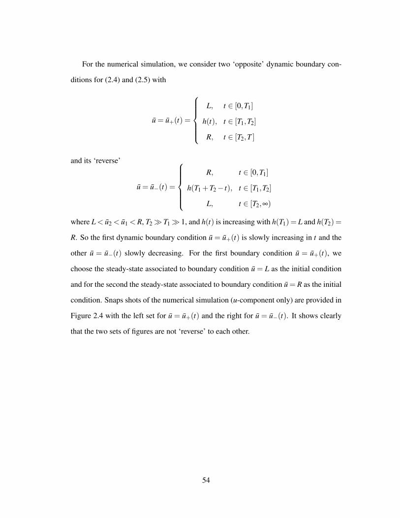
For the numerical simulation, we consider two ‘opposite’ dynamic boundary con-

ditions for (2.4) and (2.5) with

u = u+(t) =

L, t ∈ [0,T1]

h(t), t ∈ [T1,T2]

R, t ∈ [T2,T ]

and its ‘reverse’

u = u−(t) =

R, t ∈ [0,T1]

h(T1 +T2− t), t ∈ [T1,T2]

L, t ∈ [T2,∞)

where L < u2 < u1 < R, T2 T1 1, and h(t) is increasing with h(T1) = L and h(T2) =

R. So the first dynamic boundary condition u = u+(t) is slowly increasing in t and the

other u = u−(t) slowly decreasing. For the first boundary condition u = u+(t), we

choose the steady-state associated to boundary condition u = L as the initial condition

and for the second the steady-state associated to boundary condition u = R as the initial

condition. Snaps shots of the numerical simulation (u-component only) are provided in

Figure 2.4 with the left set for u = u+(t) and the right for u = u−(t). It shows clearly

that the two sets of figures are not ‘reverse’ to each other.

54

0

1.2

0

0

0

1.4 1.6

0.2

1.8 2

0.4

2.2 2.4

0.6

2.6

9.5

0.8

10

1

11

0

0

0

0

0

0

0

0

2

2

2

2

2

2

4

12

4

4

4

44

6

6

6

6

6

6

8

8

13

88

8

8

10

10

1010

10

10

12

14

12 12

1212

12

14.514

14

14

14

y

0.2 0.4 0.6 0.8 1

u

β

y

Figure 2.5: On the left, beginning at the bottom, the right boundary condition u is slowlyincreased. When a value of u is near a critical point u1 ≈ 10.98 or u2 ≈ 12.78, we pause theboundary condition in order to converge to a steady state. The left hand side pauses at thevalues u1

L(1) = 10.6,u2L(1) = 11.1,u3

L(1) = 12.7, and u4L(1) = 12.9 and the bottom, beginning

from the right, pauses at the values u1R(1) = 12.9,u2

R(1) = 12.6,u3R(1) = 11, and u4

R(1) = 10.7.

55

Chapter 3

Shearing Flows in the Leslie-Ericksen Continuum

Theory of Nematic Liquid Crystals

In this chapter we consider a one-dimensional shearing flow within the context of the

Leslie-Ericksen continuum theory of liquid crystals. In this shearing flow, a nematic

liquid crystal layer is confined between two parallel plates a distance 2h apart with the

velocity field parallel to the plates and the velocity gradient perpendicular to the plates.

We assume the velocity and director fields are of the form

v(t,y) = 〈v(t,y),0,0〉, (3.1)

n(t,y) = 〈cos(θ(t,y)),sin(θ(t,y)),0〉 (3.2)

where θ is the angle between the x-axis and the director field. Notice, that |n|= 1.

We now reformulate the governing equations (1.22)- (1.32) for this shearing flow.

We compute

∇ ·n = n2,2,

∇×n = 〈0,0,n1,2〉,

56

n ·∇×n = 0,

n× curl(n) = 〈−n2n1,2,n1n1,2,0〉,

N =12

∂v∂y〈−n2,n1,0〉+θt〈−sin(θ(t,y)),cos(θ(t,y)),0〉. (3.3)

The stress tensor terms are

toj1, j =−

∂ p∂x−

3

∑j=1

3

∑k=1

∂

∂x j

∂F∂nk, j

nk,1 =−∂ p∂x

,

toj2, j =−

∂ p∂y−

3

∑j=1

3

∑k=1

∂

∂x j

∂F∂nk, j

nk,2

=−∂ p∂y− d

dy[

∂F∂n1,2

n1,2 +∂F

∂n2,2n2,2]

=−∂ p∂y− d

dy[K3n2

1,2 +K1n22,2],

toj3, j =−

∂ p∂ z−

3

∑j=1

3

∑k=1

∂

∂x j

∂F∂nk, j

nk,3 =−∂ p∂ z

,

since nk,1 = nk,3 = 0 for all k, and

tdj1, j =

3

∑j=1

∂

∂x jtd

j1 =∂

∂yt ′21(y),

tdj2, j =

3

∑j=1

∂

∂x jtd

j2 =∂

∂yt22(y),

57

tdj3, j =

3

∑j=1

∂

∂x jtd

j3 = 0,

where

td21 = g(θ)

dvdy

+h(θ)θt ,

t22 =−2 f (θ)+14

sin(2θ)[2µ1 sin2(θ)+µ2 +µ3 +µ4 +µ5]vy−1/2hθ (θ)θt ,

h(θ) = µ3 cos2(θ)−µ2 sin2(θ),

g(θ) = µ1 cos2(θ)sin2(θ)+1/2[µ5−µ2]sin2(θ)+1/2[µ3 +µ6]cos2(θ)+1/2µ4,

f (θ) = K1 cos2(θ)+K3 sin2(θ).

In the construction of the dynamic theory, [28], Leslie shows that g > 0, which we

will assume from here on. Additionally, to simplify our analysis, we assume that f > 0.

Given the Onsager-Parodi relation, [14, 36],

µ2 +µ3 = µ6−µ5, (3.4)

we express g by the formula

2g(θ) = 2µ1 cos2(θ)sin2(θ)+µ5 +µ4 +µ3 +[µ3 +µ2]cos(2θ)

= 2µ1 cos2(θ)sin2(θ)+µ5 +µ4 +µ3−λ2 cos(2θ)

The condition g > 0 leads to the inequality

|λ2|< µ3 +µ4 +µ5. (3.5)

58

Frank’s free energy formula, (1.4), reduces to

F = K1n22,2 +0+K3n2

1,2(n22 +n2

1) = K1n22,2 +K3n2

1,2. (3.6)

Using the derived formulas of the stress tensors the component form of (1.30) is

ρvt = f1−∂ p∂x

+∂

∂ytd21(t,y),

0 = f2−∂ p∂y

+∂

∂ytd22(t,y),

0 = f3−∂ p∂ z

.

At this point we assume that the external director body force is conservative. That

is

〈 f1, f2, f3〉=−∇(χ)

for some real valued scalar potential function χ . An electromagnetic field is an example

of a conservative director body force and is used in determining Frank’s constants by

measuring the the strength of magnetic field needed to induce a Freedericksz effect,

[10, 16].

Taking the derivative of the first equation with respect to x, then substituting in the

second equation and noticing from the third equation that χ + p is independent of z

gives∂

∂ytd21(t,y)+A = ρvt ,

and

(χ + p) = Ax+ t22(t,y)+d,

59

where

A =− ∂

∂x(χ + p).

Finally from the first of these equations we obtain

ddy

[g(θ)dvdy

+(µ3 cos2(θ(t,y))−µ2 sin2(θ(t,y)))θt ]+A = ρvt . (3.7)

To derive an equation for θ , be begin by setting ρ1 = 0; that is we assume that the

contribution of the positional movement of the director is negligible when compared to

the alignment energy, E, see equation (1.12). We also assume that there are no external

body forces, i.e. Gi = 0, i = 1,2,3. Then the component form of (1.31) is

0 = gi + s ji, j,

with

g1 = γn1−β2n1,2−1/2λ1dvdy

n2 +1/2λ2n2dvdy−λ1 sin(θ)θt

= γ cos(θ)+β2 sin(θ)θ ′+1/2(λ2−λ1)sin(θ)v′−λ1 sin(θ)θt ,

g2 = γn2−β2n2,2 +1/2λ1dvdy

n1 +1/2λ2n1dvdy

+λ1 cos(θ)θt

= γ sin(θ)−β2 cos(θ)θ ′+1/2(λ1 +λ2)cos(θ)v′+λ1 cos(θ)θt ,

g3 = 0,

60

s j1, j = β2n1,2 +K3ddy

n1,2

=−β2 sin(θ)θ ′−K3 cos(θ(y))(θ ′(y))2−K3 sin(θ(y))θ ′′(y),

s j2, j = β2n2,2 +K1ddy

n2,2

= β2 cos(θ)θ ′−K1 sin(θ(y))(θ ′(y))2 +K1 cos(θ(y))θ ′′(y),

s j3, j = 0,

where ′= d/dy. Solving for the indeterminate γ in the first equation and substituting

back into the second equation gives

0 = sin(θ)(1/2λ1v′ sin(θ)−1/2λ2v′ sin(θ)+K3 cos(θ)(θ ′)2 +K3 sin(θ)θ ′′+λ1 sin(θ)θt)

+ cos(θ)(1/2λ1v′ cos(θ)+1/2λ2v′ cos(θ)−K1 sin(θ)(θ ′)2 +K1 cos(θ)θ ′′+λ1 cos(θ)θt)

= (K3 sin2(θ)+K1 cos2(θ))θ ′′+(K3 cos(θ)sin(θ)−K1 cos(θ)sin(θ))(θ ′)2

+1/2(λ1 +λ2 cos(2θ))v′+λ1θt ,

which we express as the second order nonlinear partial differential equation

2 f (θ)θ ′′+ fθ (θ)(θ′)2 + v′(λ1 +λ2 cos(2θ))+2λ1θt = 0. (3.8)

We obtain from (3.7) and (3.8) the governing system of pdes of the nematic liquid-

crystal in shear flow

ρvt =∂

∂y[g(θ)v′+h(θ)θt ]+A, (3.9)

61

−2λ1θt = 2 f (θ)θ ′′+ fθ (θ)(θ′)2 + v′(λ1 +λ2 cos(2θ)). (3.10)

The shearing flow is completely described once we stipulate that the flow is induced

by a shearing force applied to the upper plate and that the director has a fixed orientation

on the upper and lower plate. These are the boundary conditions for (3.9) and (3.10)

v(t,−h) = 0, v(t,h) = v, (3.11)

θ(t,−h) = φ = θ(t,h). (3.12)

where 2h is the distance between the two plates and φ ∈ [0,π) since one does not

distinguish between n and −n.

With the shearing flow fully prescribed we begin an exploration of the existence,

dynamics, and stability of steady state solutions. As in Chapter 2, it is the underlying

structure in the governing equations which allows us move forward through difficulties.

The general plan of study will be as follows:

(i) Steady states: existence and uniqueness.

(ii) Stability of steady states.

(iii) Semi-global and global dynamics.

We begin the plan of study by exploring the existence of steady states. This is made

more complicated by the shear number of parameters, the Leslie coefficients and Frank

constants, as well as their interdependencies. In what follows we set up the steady state

problem and using a clever change of variables transform the system into a Hamiltonian

system. Then, we give a complete description of phase plane configurations on a subset

62

of the Leslie coefficients. Focusing in on one region in particular we then give a nec-

essary condition for the existence of a steady state solution. Even with this extensive

work we have only begun to explore the tip of the iceberg and thus end the chapter by

with a discussion of what may lie below the surface.

3.1 The steady state system

In the steady state, θt = 0,vt = 0, equations (3.9) and (3.10) reduce to the system of

nonlinear ordinary differential equations

M = g(θ)v′+Ay (3.13)

0 = 2 f (θ)θ ′′+ fθ (θ)(θ′)2 + v′(λ1 +λ2 cos(2θ)) (3.14)

where M = td21(h) and subject to the boundary conditions

v(−h) = 0, v(h) = v, θ(−h) = φ = θ(h). (3.15)

Assuming the absence of external director body forces, i.e. A = 0, equation (3.13) is

integrable. Thus the velocity is given by

v(t) =ˆ t

−h

Mg(θ(τ))

dτ.

From this we see that the study of system (3.13),(3.14) reduces to the study of equation

(3.14).

Set

θ′ =

η

f (θ).

63

Under this transformation (3.14) can be written as the system of odes

θ′ =

1f (θ)

η

η′ =

fθ (θ)

2 f (θ)2 η2− v′

2(λ1 +λ2 cos(2θ))

(3.16)

Theorem 3. The system (3.16) is a Hamiltonian system with a Hamiltonian function

given by

H(θ ,η) =1

2 f (θ)η

2 +MG(θ) (3.17)

where G(θ) =

ˆλ1 +λ2 cos(2θ)

4g(θ)dθ is an antiderivative.

3.2 Phase plane configurations

In this section we analyze the phase plane associated with system (3.16) and give a

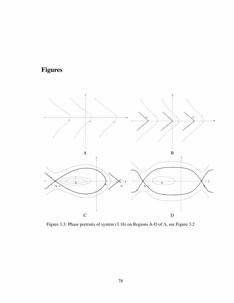
complete characterization with respect to the parameter space Λ = (λ1,λ2) ∈ R2,

where λ1,λ2 are defined in (1.28)

If |λ2|< |λ1| the system contains no equilibrium on the η-axis. It is in this region,

(λ1,λ2) : |λ2| < |λ1|, that solutions of (3.16) cannot undergo multiple twists within

the channel. Yet, there is still the possibility for a multiplicity of solutions, which is a

topic for further research.

Now suppose that either |λ1| < |λ2| or |λ1| = |λ2| and let θ0 be the unique value

[0,π/2) such that cos(2θ0) =−λ1λ2

. System (3.16) possess fixed points with η = 0 and

θ = θ0± kπ

or

θ =−θ0± kπ,

64

for all k ∈ Z. The linearization about the fixed points (θ0 + kπ,0) is

x′ =

0 [ f (θ0)]−1

Mλ2g(θ0)

sin(2θ0) 0

x, (3.18)

which has eigenvalues

µ =±

√cλ2 sin(2θ0)

f (θ0)g(θ0)

and the eigenvalues of the linearization about the fixed points (−θ0 + kπ,0) are

µ =±

√−cλ2 sin(2θ0)

f (θ0)g(θ0).

We see that the eigenvalues of the linearizations are independent of λ1 allowing us

to give a complete characterization of fixed points based upon the sign of λ2. The fixed

points (θ0 + kπ,0) are hyperbolic if λ2 > 0 and are centers if λ2 < 0. The fixed points

(−θ0 + kπ,0) are centers if λ2 < 0 and hyperbolic if λ2 > 0.

In order to analyze the phase plane on the region Λ>, defined by

Λ> = (λ1,λ2) ∈ R2 : 0 < |λ1|< |λ2|, (3.19)

we introduce the function F : Λ>→ R given by the formula

F(λ1,λ2) =

ˆπ

0

λ1 +λ2 cos(2t)2g(t)

dt. (3.20)

By symmetry and π-periodicity of the functions g(t) and cos(2t), we compute an alter-

nate form

F(λ1,λ2) = 2ˆ π

4

0

λ1(2µ1 cos2(t)sin2(t)+µ3,4,5)+λ 22 cos2(2t)

g(t)g+(t)dt, (3.21)

65

where µ3,4,5 = µ3 +µ4 +µ5 and g+(t) = g(t +π/2).

Without loss of generality we take G(θ) in Theorem 3 to be

G(θ)≡ G(θ ,λ1,λ2) =

ˆθ

θ0−π

λ1 +λ2 cos(2t)4g(t)

dt. (3.22)

Then, by construction

F(λ1,λ2) = 2G(θ0). (3.23)

Now, fix λ2 > 0, then

G′(θ) =λ1 +λ2 cos(2t)

4g(t)

< 0, if θ0−π < θ <−θ0

= 0, if θ =−θ0

> 0, if −θ0 < θ < θ0

(3.24)

for all (λ1,λ2) ∈ Λ>.

The saddle point (θ0− π,0) lies on the level curve with H(θ0− π,0) = G(θ0−

π,λ1,λ2) = 0, Theorem 3. Thus, if 0 = F(λ1,λ2), then equations (3.24), (3.23), and

Theorem 3 together imply that there exists a herteroclinic orbit from the point (θ0−

π,0) to the point (θ0,0), and by symmetry a heteroclinic orbit from the point (θ0,0) to

the point (θ0−π,0). Furthermore, since λ2 > 0, then θ0 ∈ (0,π/4) and so

θ0−π < 0 < θ0.

If F(λ1,λ2)> 0, then by the same arguments used above there exists a unique value

θh ∈ (−θ0,θ0) such that G(θh) = 0, Figure 3.1 (a). Hence H(θh,0) = 0, which proves

the existence of a homoclinic orbit to (θ0−π,0) containing the point (θh,0).

66

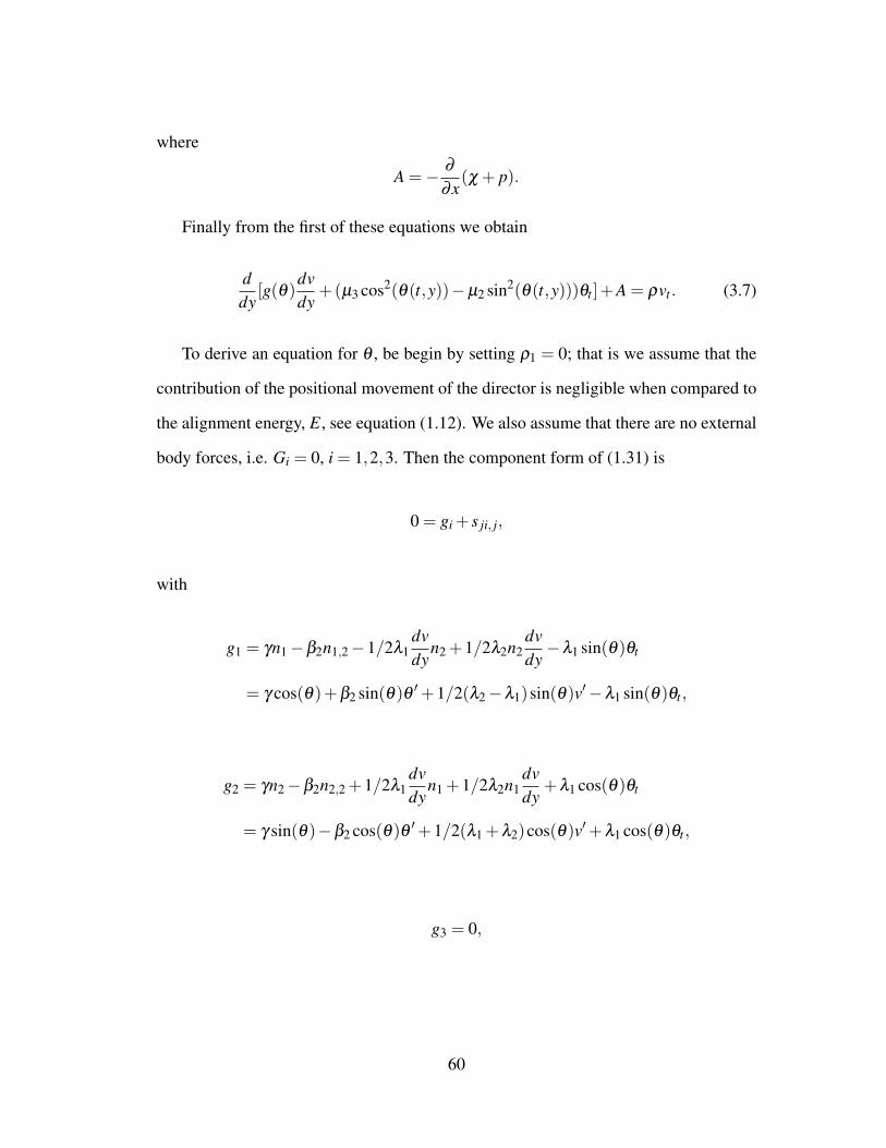
On the other hand, if F(λ1,λ2) < 0, then there exists a unique value θh ∈ (θ0−

π,−θ0) such that G(θh) = G(θ0), Figure 3.1(b). Hence H(θ0,0) = H(θh,0), which

proves the existence of a homoclinic orbit to (θ0,0) containing the point (θh,0).

θh

θ0−π θ0−θ0 θh θ0−θ0θ0−π

(a) (b)

Figure 3.1: Graphs of G(θ) with (a) F(λ1,λ2)> 0 and (b) F(λ1,λ2)< 0.

We now show that each of these cases can be realized in Λ>.

Lemma 15. With F defined above, there exists a C1 curve h : R+ → R such that

(h(λ2),λ2) ∈ Λ> and

F(h(λ2),λ2) = 0

for all λ2 ∈ (0,∞). Furthermore, for all (λ1,λ2) ∈ Λ>0,

F(λ1,λ2)> 0 if λ1 > h(λ2)

and

F(λ1,λ2)< 0 if λ1 < h(λ2).

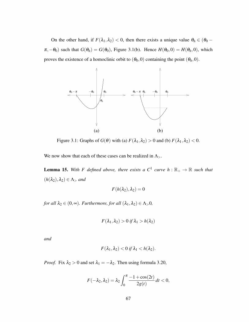
Proof. Fix λ2 > 0 and set λ1 =−λ2. Then using formula 3.20,

F(−λ2,λ2) = λ2

ˆπ

0

−1+ cos(2t)2g(t)

dt < 0,

67

and by continuity F(λ1,λ2)< 0 for λ1 ≈−λ2. Similarly F(λ1,λ2)> 0 for λ1 ≈ λ2.

By the Intermediate Value Theorem there exists a λ ∗1 such that −λ2 < λ ∗1 < λ2 and

F(λ ∗1 ,λ2) = 0.

Now,

Fλ1 =

ˆπ

0

12g(t)

dt > 0,

and thus by the implicit function theorem there exists an ε > 0 and a C1 function h :

(λ2−ε,λ2+ε)→R such that h(λ2)= λ ∗1 and F(h(τ),τ)= 0 for all τ ∈ (λ2−ε,λ2+ε).

Since λ2 was fixed arbitrarily, then the function h can be smoothly extended to all of

R+.

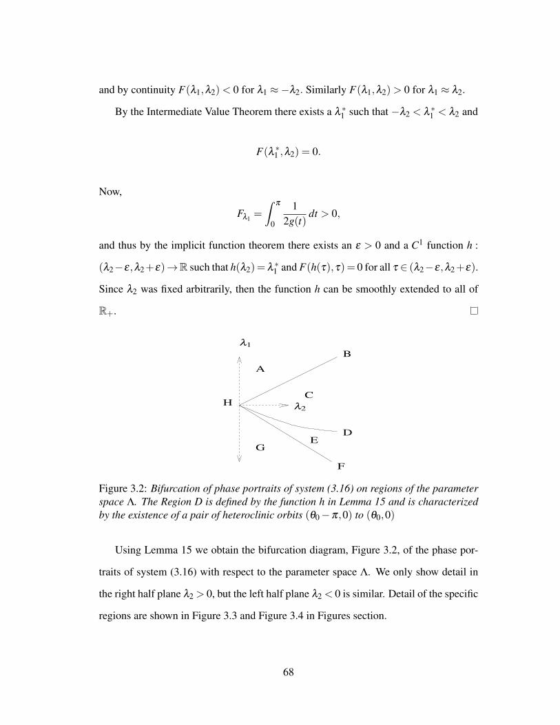
CH

B

DE

F

A

G

λ1

λ2

Figure 3.2: Bifurcation of phase portraits of system (3.16) on regions of the parameterspace Λ. The Region D is defined by the function h in Lemma 15 and is characterizedby the existence of a pair of heteroclinic orbits (θ0−π,0) to (θ0,0)

Using Lemma 15 we obtain the bifurcation diagram, Figure 3.2, of the phase por-

traits of system (3.16) with respect to the parameter space Λ. We only show detail in

the right half plane λ2 > 0, but the left half plane λ2 < 0 is similar. Detail of the specific

regions are shown in Figure 3.3 and Figure 3.4 in Figures section.

68

Notice that for λ2 fixed, as we vary the value of λ1, the value of θ0 varies as well.

More specifically θ0→ π/4− as λ1→−λ+2 and θ0→ 0+ as λ1→ 0−.

3.3 Existence in the region containing 5CB

Two of the most well studied nematic liquid crystals 4-mthoxybenzylidene-4’-butylaniline

(MBBA) and 4-pentyl-4’cyanobiphenyl (5CB) have parameter sets which lie in the the

region E shown in Figure 3.2; the values of the Leslie coefficients and Franks constants

for 5CB and MBBA can be found in [44] Appendix D. Thus we study the region E

as a jumping off point of in our study of steady state solutions subject to to the strong

anchoring boundary condition

θ(−h) = 0 = θ(h). (3.25)

Physically the boundary condition (3.25) is such that the liquid crystal lies on the upper

and lower plate in a direction parallel to the plates. We rely on the time map method

for our analysis and so before continuing we give a brief overview of this now.

3.3.1 The time map technique

The time map technique developed in a series of papers by Smoller and Wasserman,

[42, 43, 13], as well as Brunovsky and Chow, [4], is a method for characterizing the

existence and bifurcation of steady state solutions of the reaction-difusion equation

ut = uxx + f (u), (3.26)

69

subject to Dirichlet,

u(t,−L) = 0 = u(t,L), (3.27)

or Neumann,

ux(t,−L) = 0 = ux(t,L), (3.28)

boundary conditions. Reaction-diffusion systems arises naturally as a models of chemi-

cal reactions and biological processes. It is well known that every solution of (3.26),(3.27),

which does not blow up in finite time, approaches a steady state solution as t →±∞,

[4]. Thus, it is of importance to understand the existence and multiplicity of solutions

of the steady state equation

uxx + f (u) = 0, (3.29)

subject to boundary conditions

u(−L) = 0 = u(L). (3.30)

This is exactly what the time map technique aims to accomplish by exploiting the

Hamiltonian structure of system (3.29).

We make the change of variables x ≡ Lx and set v = u′, so that we can rewrite

system (3.26) as the equivalent two dimensional linear system

u′ = v, v′ =−L2 f (u). (3.31)

The system (3.31) is called a classical Hamiltonian (Newtonian) system and the solu-

tions lie on the level curves of the Hamiltonian function

H(u,v) =v2

2+L2F(u), (3.32)

70

where F(u) is an antiderivative of f (u) and without loss of generality we assume

F(0) = 0. Now suppose that (u(x),v(x)) is a solution of (3.31) lying on the level curve

H(u,v) = ξ , ξ > 0, with initial condition (u(0),v(0)) = (0,√

2ξ ). Suppose this solu-

tion intersects the positive x-axis at a point (α,0), α > 0. Then the time map is defined

by

T (α) = inf t > 0 : u(t) = α,v(t) = 0, (3.33)

and is such that (u(T (α)),v(T (α))) = (α,0) and for 0 < x < T (α), v(x) > 0. Fur-

thermore, by symmetry it is also true that (u(2T (α)),v(2T (α))) = (0,−√

2ξ ). The

existence of a solution to (3.29),(3.30) boils down to showing that there exists and α in

the domain of T such that T (α) = 2L.

The characterization of multiplicity of steady state solutions is done through ana-

lyzing the derivatives of the time map. Examples of this can be found in the works of

SH Wang and Kazarinoff, [46], in the case of the classic Kolmogorov equation

ut =12

uxx + f (u), (3.34)

where f ∈C2([0,1]) satisfies f (x)> 0 on (0,1), f (1) = 0, and there exists a small δ > 0

such that f ′(u) ≤ 0 in (1−δ ,1). More recent work via time map techniques by Qian,

[39], concerns L-periodic solutions of (3.29) and work by Z. Wang, [47], concerns

L-periodic solutions of the nonlinear equation

x′′+ f (x)x′+g(x) = e(t), (3.35)

where f ,g,e ∈C([0,∞)) and e(t) is an L-periodic forcing term.

The last few examples show that the time map technique is highly dependent of the

form of f (u) and as such work is done on a case by case basis.

71

3.3.2 Existence of single twist solutions

We proceed to set up the time map for our problem to prove the existence of a singly

twisted solution; i.e. the liquid crystal undergoes a single twist in the channel. Suppose

that (θ(y),η(y)) is a solution of (3.16) satisfying the boundary condition

θ(−h) = φ = θ(h) (3.36)

for fixed φ ∈ [−θ0,θ0). Without loss of generality we take G in Theorem 3 to be

G(θ) =

ˆθ

−θ0

λ1 +λ2 cos(2s)4g(s)

ds. (3.37)

Now suppose that the solution (θ(y),η(y)) with initial condition (θ(0),η(0)) = (φ ,ξ ),

ξ > 0 , traversing in a clockwise manner, intersects the θ -axis for the first time at a point

(α,0). In region E, these types of solutions always exist and lie inside the homoclinic

orbit to (θ0,0), see Figure 3.4 in Figures section.

By our choice of G, this solution lies on the level set H(α,0), given by

MG(α) =1

2 f (θ)η

2 +MG(θ). (3.38)

Since η = θ ′ f (θ) then using separation of variables in (3.38) we have

y =2√M

ˆθ(y)

φ

√f (t)√

G(α)−G(t)dt,

from which we are able to derive the explicit form of the time map given by

T (α) =2√M

ˆα

φ

√f (t)√

G(α)−G(t)dt. (3.39)

72

By construction the time map is such that (θ(T (α)),η(T (α))) = (α,0) and by sym-

metry (θ(2T (α)),η(2T (α))) = (φ ,−ξ ).

Making the linear change of variables t ≡ l(u,α) = αu+(1−u)φ we have

√M2

T (α) = (α−φ)

ˆ 1

0

√f (l(u,α))√

G(α)−G(l(u,α))du, (3.40)

and

√M2

T ′(α) =

ˆ 1

0

f (l(u,α))(G(α)−G(l(u,α)))√f (l(u,α))(G(α)−G(l(u,α))3/2

du

+α−φ

2

ˆ 1

0

u f ′(l(u,α))(G(α)−G(l(u,α))− f (l(u,α))(G′(α)−uG′(l(u,α))√f (l(u,α))(G(α)−G(l(u,α))3/2

du

=

ˆ 1

0

f (l(u,α))[ϕ(α)−ϕ(l(u,α))]+ α−φ

2 u f ′(l(u,α))(G(α)−G(l(u,α))√f (l(u,α))(G(α)−G(l(u,α))3/2

du,

where

ϕ(t) = G(t)− t2

G′(t),

and

f ′(t) = 2(K3−K1)cos(t)sin(t) = (K3−K1)sin(2t).

The time map we constructed is generic for solutions inside the homoclinic orbit,

but properties of the time map, T , depend on the choice of boundary conditions φ . We

show the existence of a single twist solution for φ ≥−θ0,

Lemma 16. Suppose that K3 > K1, µ1 > 0, and λ1,λ1 lie in region E. If φ > −θ0,

then the minimum time, h, it takes for a solution (θ(y),η(y)) satisfying 0 ≤ η(0) <√2M f (θ0)G(θ0) and (θ(h),η(h)) = (α,0) is given byT (α) which satisfies

(i) T ′(α)> 0 for α ∈ (φ ,θ0)

73

(ii) limα→φ+

T1(α) = 0

(iii) limα→θ

−0

T1(α) = ∞

Proof. Since we are in region E, θ0 ∈ (0,π/4). The condition 0≤η(0)<√

2M f (θ0)G(θ0)

guarantees that the solution is periodic lying inside the homoclinic orbit to (θ0,0). To

prove the first part of the lemma is suffices to show that ϕ ′(t) > 0 for t ∈ (−θ0,θ0)

since K3 > K1 and G(α)−G(l(u,α))> 0. We compute

2g′(t) = 4µ1 cos3(t)sin(t)−4µ1 cos(t)sin3(t)+2λ2 sin(2t)

= 2µ1 sin(2t)cos(2t)+2λ2 sin(2t)

= 2sin(2t)[µ1 cos(2t)+λ2],

and so

2ϕ′(t) = G′(t)− tG′′(t)

=2g(t)(λ1 +λ2 cos(2t))+4λ2tg(t)sin(2t)+2tg′(t)(λ1 +λ2 cos(2t))

(2g(t))2

=2g(t)(λ1 +λ2 cos(2t))+ t sin(2t)[4λ2g(t)+2(µ1 cos(2t)+λ2)(λ1 +λ2 cos(2t))]

(2g(t))2 .

We see that each term in the numerator is positive and hence ϕ ′(t)> 0.

The asymptotic behavior can be proved using the fact that the solution (θ(y),η(y))

approaches the stable branch of the hyperbolic fixed point (θ0,0) as α → θ−0 . On the

other side, near φ , the denominator is bounded below, and hence the term√

α−φ

governs the asymptotic behavior.

Lemma 17. Suppose that K3 > K1, µ1 > 0, and λ1,λ2 lie in region E. If φ = −θ0,

then the minimum time, h, it takes for a solution (θ(y),η(y)) satisfying 0 ≤ η(0) <√2M f (θ0)G(θ0) and (θ(h),η(h)) = (α,0) is given by T (α) which satisfies

74

(i) T ′(α)> 0 for α ∈ (−θ0,θ0)

(ii) limα→−θ

+0

T1(α) = π

√f (θ0)g(θ0)

Mλ2 sin(2θ0)

(iii) limα→θ

−0

T1(α) = ∞

Proof. The proof of T ′ > 0 carries over from Lemma 16. The asymptotic behavior

is proved using the fact that the solution (θ(y),η(y)) approaches the stable branch

of the fixed point (θ0,0) as α → θ−0 . On the other side, as α → −θ

+0 the system

is approximated by the linearization (3.18) and hence the time it takes is one half π

the frequency which is given by the eigenvalue of the linearization at (−θ0,0). Note

one may also directly perform an asymptotic expansion of the integrand to prove this

fact.

We define

he = π

√f (θ0)g(θ0)

Mλ2 sin(2θ0). (3.41)

In order to prove the existence of a solution for the full system (3.16) with bound-

ary conditions (3.15) it is necessary to show that a solution of (3.14) with boundary

condition (3.36) exists.

Theorem 4. Suppose the hypothesis of Lemma 16, then there exists a solution of (3.14)

subject to the boundary conditions

θ(−h) = φ = θ(h)

with−θ0 < φ < θ0 which undergoes a single twist within the channel. If φ =−θ0, then

there exists a singly twisted solution if and only if h > he.

75

Proof. If φ = −θ0, then the result follows immediately from the definition of he to-

gether with Lemma 17. If θ0−π < φ < θ0 then the result follows immediately from

Lemma 16.

3.4 Further Research

There are many interesting dynamics exhibited by nematic liquid crystals in shearing

flow and we have simply scratched the surface in this chapter. A quick glance at Figure

3.2 shows that there are many types of steady state solutions which may exist satisfying

the strong anchoring boundary condition θ(−h) = φ = θ(h). These include symmet-

ric, asymmetric, and super twisted solutions, although certain regions of the parameter

space Λ and choices of Frank constants place a restriction on their existence. Thus a

more thorough analysis on the different regions of phase space configurations is needed.

In the region E, see Figure 3.2, we will focus first on the critical periodic solution

(θ(y),η(y)) which satisfies the boundary condition θ(−h) = 0 = θ(h) and θ ′(−h) =

0 = θ ′(h). This is the solution which wraps once and touches the η-axis. Treating the

length of the channel,h, as a bifurcation parameter we see that this symmetric steady

state solution has the possibility to bifurcate two asymmetric solutions. A more rigorous

analysis of the time map is needed to determine if this is a possible.

Region A is also interesting and more directly analogous to our previous work in

Chapter 2 in that on this parameter region system (3.16) contains no equilibrium points.

Moreover, while there is the possibility of multiple singly twisted steady state solutions,

there cannot exist super twisted solutions.

Similar to the study done in Chapter 2, an inspection of bifurcations of the zero

eigenvalue can be carried out by noting that the zero eigenvalue problem associated

with the linearization about a steady state is precisely the linearization about a steady

76

state. Thus we will be able to exploit the Hamiltonian structure of the steady state

system in order to better understand the spectrum in a neighborhood of the zero eigen-

value. For the bifurcation of a critical periodic solution mentioned above, the condition

θ ′(−h)= 0= θ ′(h) implies that θ ′(y) is a solution of the zero eigenvalue problem. This

is important because it shows that the zero eigenvalue may have multiplicity greater

than one, which allows for the possibility of more complex types of bifurcations.

77

Figures

θ

η

−π π

η

θ

A B

θ

θh−θ0

θ0−π θ0

η

θ−θ0

θ0θ0−π

η

C D

Figure 3.3: Phase portraits of system (3.16) on Regions A-D of Λ, see Figure 3.2

78

θ0θh

−θ0θ0−π

η

θ

−ππ

η

θ

E Fη

θ

η

θ

G H

Figure 3.4: Phase portraits of system (3.16) on Regions E-H of Λ, see Figure 3.2

79

Bibliography

[1] A. Abbot, D.S.and Voigt and D. Koll. The Jormungand global climate state andimplications for Neoproterozoic glaciations. Journal of Geophysical Research,116, 2011. Cited on 53

[2] J. Alexander, R. Gardner, and C. Jones. A topological invariant arising in thestability analysis of traveling waves. J. Reine. Angew. Math., 410:167–212, 1990.Cited on 32

[3] M. Bebendorf. A note on the Poincare inequaility for convex domains. Journalfor Analysis and its Applications, 22:751–756, 2003. Cited on 26

[4] P. Brunovsky and S.-N Chow. Generic properties of stationary steady state solu-tions of reaction diffusion equations. Journal of Differential Equations, 53:1–23,1984. Cited on 69, 70

[5] M.C. Calderer. Stability of shear flows of polymeric liquid crystals. Journal ofNon-Newtonian Fluid Mechanics, 43:351–368, 1992. Cited on 11

[6] M.C. Calderer, D. Golovaty, F.-H Lin, and C. Liu. Time evolution of nematicliquid crystals with variable degree of orientation. SIAM journal on mathematicalanalysis, 33:1033–1047, 2002. Cited on 10

[7] M.C. Calderer and C. Liu. Liquid crystal flow: Dynamic and static configurations.SIAM Journal of Applied Mathematics, 60 no. 6:1925–1949, 2000. Cited on 10

[8] M.C. Calderer and C. Liu. Poiseuille flow of nematic liquid crystals. InternationalJournal of Engineering Science, 38(910):1007 – 1022, 2000. Cited on 10

[9] T. Carlson and F.M. Leslie. The development of theory for flow and dynamiceffects for nematic liquid crystals. Liquid Crystals, 26:1267–1280, 1999. Citedon 2

[10] S. Chandrasekhar. Liquid Crystals. Cambridge University Press, 2 edition, 1992.Cited on 5, 59

[11] C.H.A. Cheng, L.H. Kellogg, S. Shkoller, and D. L. Turcotte. A liquid-crystal model for friction. Proceedings of the National Academy of Sciences,105(23):7930–7935, 2008. Cited on 12, 13, 14, 15

80

[12] A. Chorin and J. Marsden. A mathematical introduction to fluid mechanics.Springer-Verlag, 3rd edition, 1992. Cited on 5, 7

[13] C. Conley and J. Smoller. Remarks on the stability of steady-state solutions ofreaction-diffusion equations. Bifurcation Phenomena in Mathematical Physicsand Related Topics: proceedings of the NATO Advanced Study Institute., pages47–56, 1980. Cited on 69

[14] P.K. Currie. Parodi’s relation as a stability condition for nematics. Molecularcrystals and liquid crystals, 28:197, 1974. Cited on 58

[15] P.K. Currie and G.P. MacSithigh. The stability and dissipation of solutions forshearing flow of nematic liquid crystals. The Quarterly Journal of Mechanics andApplied Mathematics, 32(4):499–511, 1979. Cited on 11

[16] F.P. Da Costa, E.G. Gartland, M. Grinfeld, and J. T. Pinto. Bifurcation analysisof the twist-Freedericksz transition in a nematic liquid-crystal cell with pre-twistboundary conditions. European Journal of Applied Mathematics, 20(03):269–287, 2009. Cited on 59

[17] C. Denniston, E. Orlandini, and J.M. Yeomans. Simulations of liquid crystals inPoiseulle flow. Computational and Theoretical Polymer Science, pages 389–395,2001. Cited on 53

[18] J.L. Ericksen. Equilibrium theory of liquid crystals. Advances in Liquid Crystals,2:233–298, 1976. New York: Academic Press. Cited on 5

[19] F.C. Frank. On the theory of liquid crystals. Trans. Faraday Soc., 25:19–28, 1958.Cited on 2

[20] R. Gardner and K. Zumbrun. The gap lemma and geometric criteria for instabilityof viscous shock profiles. Communications on Pure and Applied Mathematics,51(7):797–855, 1998. Cited on 32

[21] A. Ghazaryan and C. Jones. On the stability of high Lewis number combustionfronts. Discrete Contin. Dyn. Syst., 24:809–826, 2009. Cited on 32

[22] P.D. Hislop and I.M. Sigal. Introduction to Spectral Theory. Springer-Verlag,1996. Cited on 30

[23] C. Jones. Stability of the traveling wave solution of the FitzHugh-Nagumo system.Trans. Amer. Math. Soc., 286:431–469, 1984. Cited on 32

[24] T. Kapitula. The Evans function and generalized Melnikov integrals. SIAM J.Math Anal., 30:237–297, 1998. Cited on 13, 32

81

[25] T. Kapitula and B. Sandstede. Eigenvalues and resonances using the Evans func-tion. Discrete Contin. Dyn. Syst., 10:857–869, 2004. Cited on 13, 32

[26] T. Kato. Perturbation Theory for Linear Operators. Springer-Verlag, 1980. Citedon 30

[27] F.M. Leslie. Some constitutive equations for liquid crystals. Archive for RationalMechanics, 28:265–283, 1968. Cited on 5

[28] F.M. Leslie. Theory of flow phenomena in liquid crystals. Advances in liquidcrystals, 4:1–81, 1979. New York: Academic Press. Cited on 5, 7, 9, 58

[29] F.M. Leslie. Liquid crystals with variable degrees of orientation. Archive forRational Mechanics, 113:97–120, 1991. Cited on 10

[30] F.-H Lin. On nematic liquid crystals with variable degree of orientation. Commu-nications on pure and applied mathematics, 44:453–468, 1991. Cited on 10

[31] F.-H Lin, J. Lin, and C. Wang. Liquid crystal flows in two dimensions. Archivefor Rational Mechanics & Analysis, 197(1):297 – 336, 2010. Cited on 10

[32] F.-H Lin and C. Liu. Existence of solutions for the Ericksen-Leslie system. Arch.Rat. Mech. Anal, 154:135–158, 2000. Cited on 10

[33] J.G. McIntosh, F.M. Leslie, and D.M. Sloan. Stability for shearing flow of nematicliquid crystals. Continuum Mechanics and Thermodynamics, 9:293–308, 1997.10.1007/s001610050072. Cited on 11

[34] H. Millar and G. McKay. Director orientation of a twisted nematic under theinfluence of an in-plane magnetic field. Molecular Crystals and Liquid Crystals,435:937–946, 2005. Cited on 10

[35] C.W. Oseen. The theory of liquid crystals. Trans. Faraday Soc., 29:883–899,1933. Cited on 2

[36] O. Parodi. Stress tensor for a nematic liquid crystal. Le Journal de physique,31:581, 1970. Cited on 58

[37] R. Pego and M. Weinstein. Evans’ function, Melnikov’s integral, and solitarywave instabilities. Differential Equations with Applications to MathematicalPhysics, Academic Press, Boston, pages 273–286, 1993. Cited on 32

[38] L. Perko. Differential Equations and Dynamical Systems. Springer-Verlag, 3rdedition, 2001. Cited on 25, 32

[39] D. Qian. Periodic solutions for second order equations with time-dependentpotential via time map. Journal of Mathematical Analysis and Applications,294:361–372, 2003. Cited on 71

82

[40] B. Sandstede. Stability of traveling waves. Handbook of dynamical systems II,2:983–1055, 2002. Cited on 32

[41] B. Sandstede and A. Scheel. Evans function and blow-up methods in criticaleigenvalue problems. Discrete Contin. Dyn. Syst., 10:941–964, 2004. Cited on 32

[42] J. Smoller and A. Wasserman. Global bifurcation of steady-state solutions. Jour-nal of Differential Equations, 39:269–290, 1981. Cited on 69

[43] J. Smoller and A. Wasserman. Generic bifurcation of steady-state solutions. Jour-nal of Differential Equations, 52:432–438, 1984. Cited on 69

[44] I. Stewart. The static and dynamic continuum theory of liquid crystals: a mathe-matical introduction. Taylor & Francis Inc, 2004. Cited on 5, 69

[45] E.G. Virga. Variational Theories for Liquid Crystals. Chapman & Hill, 1st edition,1994. Cited on 5

[46] S. Wang and N.D. Kazarinoff. Bifurcation and stability of positive solutions ofa two-point boundary value problem. Australian Mathematical Society, 52:334–342, 1992. Cited on 71

[47] Z. Wang. Periodic solutions of the second-order forced Lienard equation via timemaps. Nonlinear Analysis, 48:445–460, 2002. Cited on 71

[48] H. Zocher. Uber die Molekulanordnung in der anisotrop-fussigen Phase. Physik.Z., 28:790, 1927. Cited on 2

[49] H. Zocher. The effect of a magnetic field on the nematic state. pubs.rsc.org, pages945–967, 1933. Cited on 2

83