Page 1
Beyond the Standard Model Effective Field Theory:
The Singlet Extended Standard Model
Shekhar Adhikari,∗ Ian M. Lewis,† and Matthew Sullivan‡
Department of Physics and Astronomy,
University of Kansas, Lawrence, Kansas, 66045 U.S.A.
Abstract
One of the assumptions of simplified models is that there are a few new particles and interactions
accessible at the LHC and all other new particles are heavy and decoupled. Effective field theory
(EFT) methods provide a consistent method to test this assumption. Simplified models can be
augmented with higher order operators involving the new particles accessible at the LHC. Any UV
completion of the simplified model will be able to match onto these beyond the Standard Model
EFTs (BSM-EFT). In this paper we study the simplest simplified model: the Standard Model
extended by a real gauge singlet scalar. In addition to the usual renormalizable interactions, we
include dimension-5 interactions of the singlet scalar with Standard Model particles. As we will
show, even when the cutoff scale is 3 TeV, these new effective interactions can drastically change
the interpretation of Higgs precision measurements and scalar searches. In addition, we discuss
how power counting in a BSM-EFT depends strongly on the processes and parameter space under
consideration. Finally, we propose a χ2 method to consistently combine the limits from new
particle searches with measurements of the Standard Model. Unlike imposing a hard cut off on
heavy resonance rates, our method allows fluctuations in individual channels that are consistent
with global fits.
∗Electronic address: [email protected] †Electronic address: [email protected] ‡Electronic address: [email protected]
1
arX
iv:2
003.
1044
9v1
[he
p-ph
] 2
3 M
ar 2
020
Page 2
I. INTRODUCTION
The Large Hadron Collider (LHC) has had two very successful runs. While no new physics
beyond the Standard Model (BSM) has been discovered, we may yet expect it to show up in
currently unanalyzed data or in future runs at the LHC. In the absence of discoveries of more
complete models such as Supersymmetry, extra dimensions, or composite Higgs models, it
is useful to study simplified models [1]. A frequent assumption of simplified models is that
there are at most a handful of new particles accessible at LHC energies, while all additional
new particles are too heavy to be produced. However, this raises the question: can the effects
of the inaccessible new particle be truly neglected? For example, consider a simplified model
with a new up-type vector like quark (VLQ). If there is a new scalar in the theory, even if
the scalar cannot be directly produced, it can mediate new loop level decays of the VLQ into
photons and gluons [2]. Indeed, in certain regions of parameter space, these decay modes
can be dominant [2–4], fundamentally changing the phenomenology of the simplified VLQ
model.
The most “model independent” method to determine the effects of new, heavy particles
is an effective field theory (EFT). An EFT is a power expansion in inverse powers of some
new physics scale Λ:
L = Lren +∞∑n=5
∑k
fk,nΛn−4Ok,n, (1)
where fk,n are Wilson coefficients, Lren is the renormalizable Lagrangian, and Ok,n are
dimension-n operators. In the Standard Model EFT (SMEFT) [5–7], Lren and Ok,n con-
sist of SM fields and are invariant under SM symmetries. To test the stability of simplified
models against heavy new physics, this frame needs to be extended to the Beyond the Stan-
dard Model EFT (BSM-EFT) [2–4, 8–15]. In the BSM-EFT, Lren and Ok,n consist of SM
and simplified model fields and are invariant under the symmetries of the simplified model.
This approach is agnostic about the high scale new physics since any UV completion of a
simplified model will match onto the BSM-EFT.
In this paper we study the BSM-EFT of the simplest possible extension of the SM, the
addition of a real scalar singlet S [16–18]. Beyond being the simplest extension of the SM,
the singlet model can help provide a strong first order electroweak phase transition necessary
of electroweak baryogenesis [19–23]. At the renormalizable level, the new singlet only enters
2
Page 3
the scalar potential and its interactions with fermions and gauge bosons are inherited by its
mixing with the SM Higgs boson. However, it is highly unlikely that a singlet scalar singlet
would appear without any new physics. For example, even if it can give rise a strong first
order electroweak phase transition, in order to successfully have electroweak baryogenesis
new sources of CP violation are needed [24–27]. In fact, it has been shown [28–30] that the
BSM-EFT for the real scalar singlet can provide the CP violation necessary for electroweak
baryogenesis.
Our analysis will consist of two major portions: re-interpreting Higgs precision measure-
ments in the singlet extended SM and re-interpreting searches for new heavy scalars. After
EWSB, the new singlet scalar and Higgs boson will mix. Without the new EFT interactions,
this mixing results in a universal suppression of Higgs boson production rates. Hence, Higgs
precision measurements have a very simple interpretation [31–35]. However, the BSM-EFT
will introduce new interactions between the Higgs boson and fermions/gauge bosons. As we
will show, these can significantly alter the interpretation of Higgs measurements. A similar
argument can be made for constraints coming from heavy scalar searches. At the renormaliz-
able level, the new scalar inherits all of its interactions with fermions and gauge bosons from
the SM Higgs boson. Hence, its production rates are the same as a heavy Higgs boson but
suppressed by a mixing angle. Similarly, its decay rates are the same as a heavy Higgs boson
suppressed by a mixing angle, except when a di-Higgs resonance is kinematically available.
That is, at the renormalizable model, the phenomenology is well defined. As we will show,
with the introduction of new interactions between the scalar and fermions/gauge bosons the
phenomenology can significantly change. Even though it is typically assumed that heavy
new physics can be neglected, we will show that even in the simplest of all simplified models
this assumption must be called into question.
This paper is an extension of work in Ref. [8], where only effective interactions between
the scalar singlet and gauge bosons were considered. We should note that the full BSM-EFT
was considered in Ref. [9]. However, they also considered dimension-6 SMEFT operators.
While these effects can be important, we are interested in the question of how the EFT
including new particles can change the phenomenology of the simplified models. Hence, we
will focus on dimension-5 operators involving SM gauge bosons, SM fermions, and the new
scalar singlet. In addition, we will include the most up-to-date Higgs precision data and
searches for scalar singlets. Also, we give a robust discussion of power counting the BSM-
3
Page 4
EFT and propose a new χ2 analysis to combine heavy resonance searches with precision
measurements.
In Section II we develop the BSM-EFT for the real scalar singlet. The EFT power
counting in a BSM-EFT can change from the usual SMEFT power counting, as we will
discuss in Sec. III. The effects of the new operators on Higgs production and decay are
shown in Sec. IV, and results from fitting to Higgs signal strengths are given in Sec. V. In
Sec. VI A we propose a χ2 analysis for heavy resonance search limits, and in Sec. VI B the
final results of heavy scalar resonances and their combination with Higgs signal strengths
are given. We conclude in Sec. VII. The Feynman rules are given in Appendix A, the
experimental results we fit to are given in App. B, and various parameter space limits are
given in App. C.
II. MODEL
We consider the SM extended by a real gauge singlet scalar, S, and will not impose an
additional Z2 upon S. In order to focus on the effects of new physics on the scalar singlet
properties, we will consider only dimension-5 EFT operators. For simplicity, we will also
only focus on CP even operators. These are the lowest order effective operators that include
a scalar singlet [8, 9]. At dimension-5, the only SMEFT operators are those that contribute
to Majorana neutrino masses [5, 6, 36], which are not relevant for LHC analyses. Hence,
these will be neglected and the BSM-EFT will only consist of operators including the new
singlet scalar.
Adapting the notation of Refs. [37], to or Λ−1 the scalar potential is:
V (Φ, S) = −µ2Φ†Φ + λ(Φ†Φ)2 +a12
Φ†ΦS +a22
Φ†ΦS2 +a32Λ
Φ†ΦS3 +a42Λ
(Φ†Φ)2S
+b1S +b22S2 +
b33S3 +
b44S4 +
b55ΛS5 (2)
where Φ = (0, φ0/√
2)T is the SM Higgs doublet in the Unitary gauge, φ0 = h + v is the
neutral scalar component of Φ, h is the Higgs boson, and 〈φ0〉 = v is the SM Higgs vacuum
expectation value (vev). Since S is not charged under any symmetry, its vev does not
break any symmetry and results in an unphysical redefinition of parameters [34, 37]. Hence,
without loss of generality we can impose 〈S〉 = 0.
4
Page 5
After electroweak symmetry breaking (EWSB), the Higgs boson h and scalar singlet have
the same quantum numbers and can mix:h1h2
=
cos θ sin θ
− sin θ cos θ
hS
, (3)
where h1,2 are mass eigenstates with masses m1,2. We will assume m1 = 125 GeV < m2,
since the other mass hierarchy is strongly constrained by LEP [31]. With the masses, mixing,
and vevs, we can now solve for five parameters in the potential
µ2 =1
2
(cos2 θm2
1 + sin2 θm22
)(4)
λ =cos2 θm2
1 + sin2 θm22
2 v2
a1 = sin 2θm2
1 −m22
v− a4
v2
Λ
b1 =1
4sin 2θ v
(m2
2 −m21
)+ a4
v4
8 Λ
b2 = cos2 θm22 + sin2 θm2
1 −1
2a2 v
2.
These are O(v/Λ) corrections on the relationships founds in Refs. [34, 37]. The free param-
eters of the scalar potential are then
m1 = 125 GeV, m2, v = 246 GeV, 〈S〉 = 0, θ, a2, a3, a4, b3, b4, b5. (5)
The scalar potential gives rise to important trilinear scalar couplings after EWSB:
V (h1, h2) ⊃1
3!λ111h
31 +
1
2λ211h
21h2, (6)
where
λ111 =3m2
1
vcos3 θ + 2 b3 sin3 θ + 3 a2v cos θ sin2 θ +
3 a3v2
2 Λsin3 θ +
3 a4v2
Λcos2 θ sin θ (7)
λ211 = −m22 + 2m2
1
vcos2 θ sin θ + 2 b3 cos θ sin2 θ + a2v sin θ
(2 cos2 θ − sin2 θ
)+
3 a3v2
2 Λcos θ sin2 θ +
a4v2
Λcos θ
(cos2 θ − 2 sin2 θ
). (8)
When kinematically allowed, the coupling λ211 gives rise to resonant double Higgs production
via the decay h2 → h1h1. The Higgs trilinear coupling λ111 can alter the non-resonant di-
Higgs rate away from SM predictions.
5
Page 6
There are important theoretical constraints on the scalar potential, Eq. (2), to consider.
Limits from the potential effect the allowed values of λ211 and can have a significant impact
on the h2 → h1h1 branching ratio [37]. First, there are quintic terms S(Φ†Φ)2,S3Φ†Φ and
S5 that dominate at large field values and can be negative, indicating an unstable potential.
We only consider parameter space where the global minimum is inside the field value region
|S| < Λ and |φ0| < Λ and not along the boundaries. Above the cut-off scale, it assumed
new physics comes in and stabilizes the potential. Second, the potential is much more
complicated than the SM and has many different minimum even inside the allowed field
value regions. The singlet vev cannot contribute to the W and Z masses. Hence, the Higgs
vev must give the correct masses and we only consider parameter space where the global
minimum is 〈φ0〉 = v = 246 GeV and 〈S〉 = 0. Finally, in the scalar potential we require
all dimensionless parameters to be bounded by 4π and all dimensionful parameters to be
bounded by Λ.
In addition to the scalar potential, the scalar singlet obtains new interactions with SM
fermions and gauge bosons [8, 9]. Current measurements of the observed Higgs boson are
only sensitive to third generation quarks, and second and third generation leptons. Hence, we
will only consider those interactions in addition to the gauge bosons. The relevant effective
interactions in the fermion mass eigenbasis for our study are then:
LEFT ⊃g2s
16π2
fGGΛS GA
µνGA,µν +
g2
16π2
fWW
ΛSW a
µνWa,µν +
g′2
16π2S BµνB
µν (9)
−(fµΛ
mµ
vS L2ΦµR +
fτΛ
mτ
vS L3Φ τR +
fbΛ
mb
vS Q3Φ bR +
ftΛ
mt
vS Q3Φ tR + h.c.
),
where L2,3 are second and third generation lepton SU(2)L doublets, Q3 is the third generation
quark SU(2)L doublet, µR, τR, bR, tR are SU(2)L singlets, and mµ,mτ ,mb,mt are the masses
of the relevant fermions. All Wilson coefficients are assumed to be real. The Feynman rules
from Eqs. (2,9) can be found in Appendix A.
III. POWER COUNTING
In traditional SMEFT counting, the amplitude squared terms should be truncated to
the same order as the Lagrangian. As an example, consider a baryon and lepton number
6
Page 7
conserving SMEFT amplitude to dimension-81
ASMEFT ∼ Aren +1
Λ2A6,SMEFT +
1
Λ4A8,SMEFT +O(Λ−6), (10)
where Aren is the dimension-4 renormalizable amplitude, and An,SMEFT are SMEFT ampli-
tudes originating from operators at dimension-n. The amplitude squared is then
|ASMEFT| ∼ |Aren|2 +1
Λ2ArenA6,SMEFT +
1
Λ4|A6,SMEFT|2 +
1
Λ4ArenA8,SMEFT +O(Λ−6).(11)
As can be clearly seen, at the amplitude squared level the dimension-8 term is of the same
order as the dimension-6 squared term. Hence, for self-consistency, if only the dimension-6
term is included in the amplitude, then the amplitude squared should also be truncated at
O(Λ−2).
According to this argument, since the interactions in Eqs. (2,9) are truncated at
dimension-5 the amplitude squareds should be truncated at O(Λ−1). Here we note that
while this is the SMEFT procedure, in the model presented the counting is more compli-
cated due to the unknown scalar mixing angle. First, consider h1 single production and
decay. The relevant singlet scalar interactions are all dimension-5 or higher. Hence, to order
Λ−2, amplitudes for h1 production and decay are schematically
Ah1 ∼ cos θAren + cos θA6,SMEFT
Λ2+ sin θ
(A5,S
Λ+A6,S
Λ2
)+O(Λ−3), (12)
where A5,S and A6,S are, respectively, dimension-5 and dimension-6 operators involving the
scalar singlet S. Note that due to mixing among the scalars after EWSB, in the production
and decay of the mass eigenstate h1 the SMEFT and renormalizable terms are proportional
to cos θ and the singlet scalar EFT terms are proportional to sin θ. The amplitude squared
is then
|Ah1 |2 ∼ cos2 θ|Aren|2 + sin θ cos θArenA5,S
Λ(13)
+1
Λ2
(sin2 θ|A5,S|2 + sin θ cos θArenA6,S + cos2 θArenA6,SMEFT
)+O(Λ−3).
In the small mixing angle limit the SM and SMEFT contributions dominate, and the usual
power counting is valid. In the large mixing angle limit, sin θ → ±1, the cos θ terms go to
zero and the amplitude squared is
|Ah1 |2 −−−−−→| sin θ|→1
|A5,S|2
Λ2+A6,SA5,S
Λ3+O(Λ−4). (14)
1 In SMEFT, dimension-5 and dimension-7 operators violate lepton and/or baryon number [36, 38–41].
7
Page 8
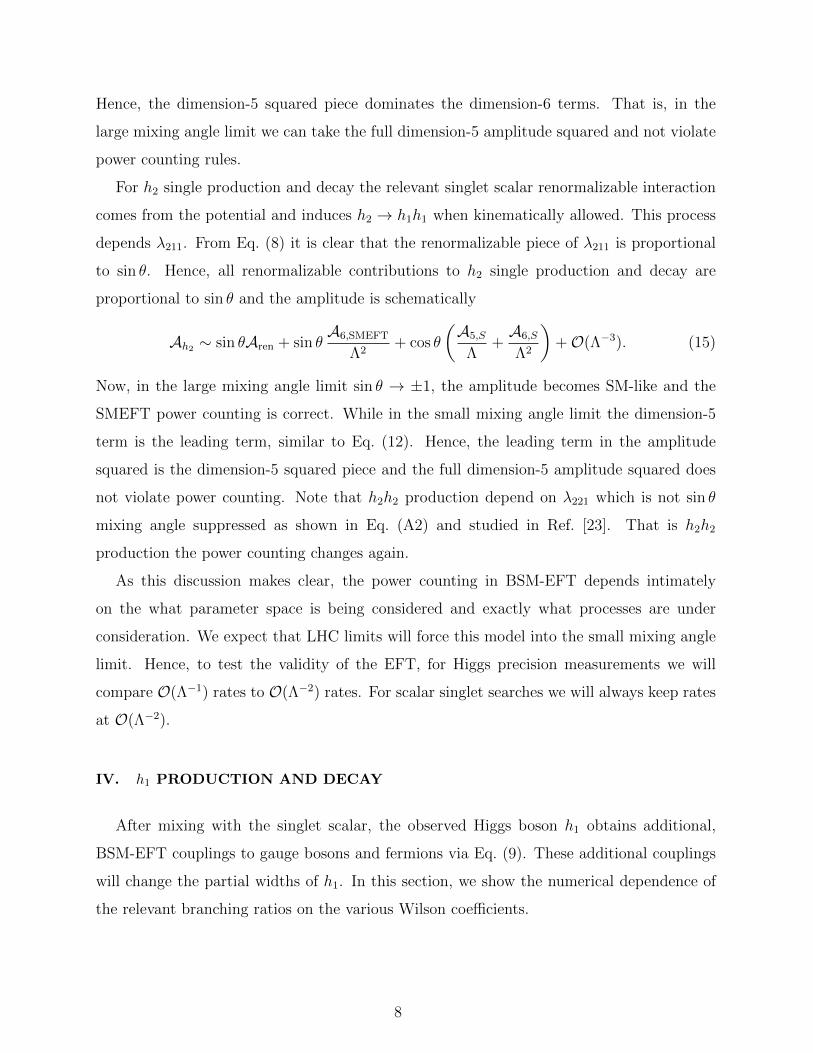
Hence, the dimension-5 squared piece dominates the dimension-6 terms. That is, in the
large mixing angle limit we can take the full dimension-5 amplitude squared and not violate
power counting rules.
For h2 single production and decay the relevant singlet scalar renormalizable interaction
comes from the potential and induces h2 → h1h1 when kinematically allowed. This process
depends λ211. From Eq. (8) it is clear that the renormalizable piece of λ211 is proportional
to sin θ. Hence, all renormalizable contributions to h2 single production and decay are
proportional to sin θ and the amplitude is schematically
Ah2 ∼ sin θAren + sin θA6,SMEFT
Λ2+ cos θ
(A5,S
Λ+A6,S
Λ2
)+O(Λ−3). (15)
Now, in the large mixing angle limit sin θ → ±1, the amplitude becomes SM-like and the
SMEFT power counting is correct. While in the small mixing angle limit the dimension-5
term is the leading term, similar to Eq. (12). Hence, the leading term in the amplitude
squared is the dimension-5 squared piece and the full dimension-5 amplitude squared does
not violate power counting. Note that h2h2 production depend on λ221 which is not sin θ
mixing angle suppressed as shown in Eq. (A2) and studied in Ref. [23]. That is h2h2
production the power counting changes again.
As this discussion makes clear, the power counting in BSM-EFT depends intimately
on the what parameter space is being considered and exactly what processes are under
consideration. We expect that LHC limits will force this model into the small mixing angle
limit. Hence, to test the validity of the EFT, for Higgs precision measurements we will
compare O(Λ−1) rates to O(Λ−2) rates. For scalar singlet searches we will always keep rates
at O(Λ−2).
IV. h1 PRODUCTION AND DECAY
After mixing with the singlet scalar, the observed Higgs boson h1 obtains additional,
BSM-EFT couplings to gauge bosons and fermions via Eq. (9). These additional couplings
will change the partial widths of h1. In this section, we show the numerical dependence of
the relevant branching ratios on the various Wilson coefficients.
8
Page 9
The total width of h1 is
Γ1 = Γ(h1 → bb) + Γ(h1 → cc) + Γ(h1 → gg) (16)
+Γ(h1 → γγ) + Γ(h1 → W±W∓,∗) + Γ(h1 → ZZ∗)
+Γ(h1 → τ+τ−) + Γ(h1 → µ+µ−).
Higher order QCD corrections are included in the numerical studies. The partial widths
Γ(h1 → bb) and Γ(h1 → cc) are calculated to next-to-next-to-leading order (NNLO) in
QCD [42–46]; and Γ(h1 → gg) [47, 48], Γ(h1 → γγ) [49–52] and Γ(h1 → Zγ) [53] are
calculated to NLO in QCD [46] by reweighting exact amplitudes by the K-factor in the
infinite top quark mass limit. Finally, for loop level decays Γ(h1 → Zγ) and Γ(h1 → γγ) we
include contributions from t, b, c, τ, µ and W , while for Γ(h1 → gg) we include t, b and c.
In addition to the Higgs boson mass, our input parameters are the same as the LHC
Higgs cross section working group [54]:
GF = 1.16637× 10⁻⁵ GeV−2, MW = 80.35797 GeV, MZ = 91.15348 GeV,
mt(mt) = 173 GeV, mb(mb) = 4.18 GeV, mc(3 GeV) = 0.986 GeV
mτ = 1.77682 GeV, mµ = 0.1056583715 GeV
αs(MZ) = 0.118,
where bars indicate MS parameters and masses inside parentheses indicate the renormaliza-
tion scale at which the parameters are evaluated. For all decays we set the renormalization
scale to the Higgs mass. All quark masses are evaluated in the MS scheme in the calculation
of the Higgs width. The conversion between on-shell and MS quantities are taken from
Ref. [46].
In Figs. 1 and 2 we show the dependence of various Higgs branching ratios and the total
Higgs width on the gauge boson and fermion Wilson coefficients with a scalar mixing angle
of sin θ = 0.1. We consider one Wilson coefficient at a time and show branching ratios for
which the Wilson coefficients make a direct contribution to the partial widths. Additionally,
deviations in the total width are important in fits to Higgs precision data since Γ1 enters
all Higgs branching ratios. Hence, we also show the dependence of the total width on the
Wilson coefficients.
From Fig. 1, it is clear that the WW and ZZ partial widths have very little dependence
on the Wilson coefficients fBB and fWW . This can be understood by noting that these
9
Page 10
-10 -5 0 5 10
fBB
/Λ (TeV-1
)
0.8
0.9
1
1.1
1.2B
R(h
1→
XY
)/B
R(h
1→
XY
) SM
XY=WW/ZZXY=γγXY=ZγΓ
1/Γ
1,SM
fWW
=fGG
=fb=f
t=fµ=fτ=0, sin θ=0.1
Solid: O(Λ-1)
Dotted: O(Λ-2)
(a)
-10 -5 0 5 10
fWW
/Λ (TeV-1
)
0.8
0.9
1
1.1
1.2
BR
(h1→
XY
)/B
R(h
1→
XY
) SM
XY=WW/ZZXY=γγ
XY=Zγ
Γ(h1)/Γ(h
1)SM
fBB
=fGG
=fb=f
t=f
µ=f
τ=0, sin θ=0.1
Solid: O(Λ-1
)
Dotted: O(Λ-2
)
(b)
-10 -5 0 5 10
fGG
/Λ (TeV-1
)
0
0.5
1
1.5
2
2.5
3
BR
(h1→
XY
)/B
R(h
1→
XY
) SM
XY=gg
Γ1/Γ
1,SM
fWW
=fBB
=fb=f
t=fµ=fτ=0, sin θ=0.1
Solid: O(Λ-1)
Dotted: O(Λ-2)
(c)
FIG. 1: Dependence of various branching ratios of h1 and h1 total width normalized to their SM
values as a function of the gauge boson Wilson coefficients (a) fBB, (b) fWW , and (c) fGG. All
other Wilson coefficients are set to zero. The partial widths are calculated at both (solid) O(Λ−1)
and (dotted) O(Λ−2). Different colors indicate different final states.
decays are tree level in the SM, while the EFT contributions are suppressed by a loop
factor, a small mixing angle, and a heavy scale. The situation changes for SM loop level
decays. Both h1 → γγ and h1 → Zγ depend strongly on fBB and fWW , with deviations
from SM predictions up to 15%. Similarly, h1 → gg strongly depends on fGG, with order
one deviations from the SM. Finally, the total width has little dependence on fBB and fWW
since γγ and Zγ have negligible contributions to Γ1. However, Γ1 depends more strongly on
fGG due to the larger h1 → gg partial width. These results are consistent with Ref. [8].
10
Page 11
-10 -5 0 5 10
fb/Λ (TeV
-1)
0.6
0.8
1
1.2
1.4
1.6B
R(h
1→
XY
)/B
R(h
1→
XY
) SM
XY=bbXY=gg
Γ1/Γ
1,SM
fWW
=fBB
=fGG
=ft=fµ=fτ=0, sin θ=0.1
Solid: O(Λ-1)
Dotted: O(Λ-2)
(a)
-10 -5 0 5 10
fτ/Λ (TeV-1
)
0.6
0.8
1
1.2
1.4
BR
(h1→
XY
)/B
R(h
1→
XY
) SM
XY=ττXY=γγ/ZγΓ
1/Γ
1,SM
fWW
=fBB
=fGG
=fb=f
t=fµ=0, sin θ=0.1
Solid: O(Λ-1)
Dotted: O(Λ-2)
(b)
-10 -5 0 5 10
ft/Λ (TeV
-1)
0.6
0.8
1
1.2
1.4
BR
(h1→
XY
)/B
R(h
1→
XY
) SM
XY=gg
XY=γγXY=ZγΓ
1/Γ
1,SM
fWW
=fBB
=fGG
=fb=fµ=fτ=0, sin θ=0.1
Solid: O(Λ-1)
Dotted: O(Λ-2)
(c)
FIG. 2: Same as Fig. 1 for the fermion Wilson coefficients (a) fb, (b) fτ , and (c) ft.
The branching ratios into fermionic final states depend strongly on the fermion Wilson
coefficients, as evidenced in Figs. 2(a,b). The decay to ττ varies as much as ∼ 30% from SM
predictions, while the bottom quark final state varies by around ∼ 20%. It is striking that
h1 → bb depends less on fb than h1 → ττ depends on fτ . This can be understood by noting
that the total width of h1 depends strongly on fb, but very little on fτ . Hence, the variation
in the h1 → bb partial width is somewhat compensated by the variation in Γ1. Similarly,
while the partial width of h1 → gg has little dependence on fb, the BR(h1 → bb) varies up
to ∼ 20 − 30% due to the variation in the total width. Finally, all the loop level processes
depend relatively strongly on the top quark Wilson coefficient, as seen in Fig. 2(c). In
particular, BR(h1 → γγ) and BR(h1 → gg) vary upwards of ∼ 15% and ∼ 30%,respectively.
11
Page 12
Finally, the branching ratios and widths calculated to (solid)O(Λ−1) and (dotted)O(Λ−2)
are shown in Figs. 1 and 2. For most final states and the total width, both the O(Λ−1) and
O(Λ−2) results agree well. This indicates that the BSM-EFT is valid in these regions of
parameter space. The only exception is the dependence of h1 → gg on fGG. However, as we
will show in the next section, the fits to the Higgs precision data also indicate the BSM-EFT
is valid in the allowed parameter regions.
While we do not explicitly show the variation of the Higgs production cross section, it
should be noted that gluon fusion is the main production mode. For on-shell h1 decay, the
LO gluon fusion production rate is
σggF (pp→ h1) =π2
8m1 SLΓ(h1 → gg), (17)
where the parton luminosity is
L =
∫ − ln(√τ0)
ln(√τ0)
dy g(√τ0e
y) g(√τ0e−y), (18)
where√S is the hadronic center-of-momentum energy and τ0 = m2
1/S. As show in Fig. 1(c)
and 2(c), this production rate will have a strong dependence on fGG and ft. Other sub-
dominant but important production modes are Higgs production in association with W/Z
(Wh1/Zh1) and vector-boson-fusion (VBF). The relevant Wilson coefficients for these pro-
duction modes are fBB and fWW . However, as evidenced in Figs. 1(a,b) Wh1, Zh1, and
VBF production will have little dependence on fBB and fWW .
V. HIGGS SIGNAL STRENGTHS
Now we perform a fit to the Higgs precision data. The effects of the additional interactions
on the Higgs measurements are parameterized using Higgs signal strengths:
µfi =σi(pp→ h1)
σi,SM(pp→ h1)
BR(h1 → f)
BRSM(h1 → f), (19)
where i is the initial state, f is the final state, and the subscript SM indicates SM values.
We combine the signal strengths into a chi-square:
χ2h1
=∑i,j
(µfi − µfi )
2
(δfi )2, (20)
12
Page 13
where µfi is a calculated signal strength, µfi is a signal strength measured at the LHC, and
δfi is the one standard deviation uncertainty on µfi . We combine measurements from both
ATLAS and CMS at the 13 TeV LHC. The set of signal strengths we use can be found in
Tables I and II in Appendix B.
For the gluon fusion (ggF) production rate we use Eq. (17) to calculate
σggF (pp→ h1)
σggF,SM(pp→ h1)=
Γ(h1 → gg)
ΓSM(h1 → gg), (21)
where the partial widths into gluons are calculated as discussed in Sec. (IV). We also include
Wh1, Zh1, Higgs production in association with a tt pair (tth1), Higgs production in asso-
ciation with a top plus jet or top plus W (collectively th1), and VBF. For these production
modes the model is implemented in MadGraph5 aMC@NLO [55] via FeynRules [56]. The de-
fault NNPDF2.3LO pdf sets [57] are used and the renormalization and factorization scales are
set to the sum of the final state particle masses. For the VBF mode, we apply the cuts [58]
pjT > 20 GeV, |ηj| < 5, |∆ηjj| > 3, andmjj > 130 GeV, (22)
where pjT are jet transverse momenta, ηj are jet pseudo-rapidity, ∆ηjj is the difference in
the jet pseudo-rapidity, and mjj is the di-jet invariant mass. These production and decay
modes are calculated at LO in QCD, and it is hoped that most of the QCD corrections
cancel in the ratio of the cross sections used for the signal strengths. However, it should be
pointed out that in the SMEFT, for some observables the QCD corrections can be strongly
dependent upon the EFT operators [59–62].
Once all the signal strengths are known, we perform a fit to the Wilson coefficients
and scalar mixing angle. As shown in Appendix A, the h1 → γγ decay depends on the
combination fBB+fWW but not fBB−fWW . Also, Fig. 1 shows that processes with external
W and Z bosons do not depend strongly on fWW and fBB. Hence, we define
f± =1√2
(fBB ± fWW ) . (23)
Now h1 → γγ will constrain only f+, and Wh1, Zh1,VBF, h1 → WW ∗, and h1 → ZZ∗
have negligible dependence on both f±. Hence, we set f− = 0. Also, the constraints on
h1 → µ+µ− are not yet strong and we set fµ = 0. Hence, the following parameters are fit
using just Higgs signal strengths:
sin θ, fGG, f+, fb, ft, and fτ . (24)
13
Page 14
0 2 4 6 8 10 12 14 16 18 20
fGG
/Λ (TeV-1
)
-1
-0.5
0
0.5
1si
n θ
ggF+th1+tth
1, µ to O(Λ-1
)
All µ to O(Λ-1)
All µ, rates to O(Λ-2)
All µ, rates to O(Λ-2) and |f
i| < 4 π
95% CL Higgs FitsΛ = 3 TeV
(a)
0 2 4 6 8 10 12 14 16 18 20
ft/Λ (TeV
-1)
-1
-0.5
0
0.5
1
sin θ
ggF+th1+tth
1, µ to O(Λ-1
)
All µ to O(Λ-1)
All µ, rates to O(Λ-2)
All µ, rates to O(Λ-2), and |f
i| < 4π
95% CL Higgs FitsΛ = 3 TeV
(b)
0 2 4 6 8 10 12 14 16 18 20
fb/Λ (TeV
-1)
-1
-0.5
0
0.5
1
sin θ
ggF+th1+tth
1, µ to O(Λ-1
)
All µ to O(Λ-1)
All µ, rates to O(Λ-2)
All µ, rates to O(Λ-2) and |f
i| < 4π
95% CL Higgs FitsΛ = 3 TeV
(c)
0 2 4 6 8 10 12 14 16 18 20
fτ/Λ (TeV-1
)
-1
-0.5
0
0.5
1
sin θ
ggF+th1+tth
1, µ to O(Λ-1
)
All µ to O(Λ-1)
All µ, rates to O(Λ-2)
All µ, rates to O(Λ-2) and |f
i| < 4π
95% CL Higgs FitsΛ = 3 TeV
(d)
0 2 4 6 8 10 12 14 16 18 20
f+/Λ (TeV
-1)
-1
-0.5
0
0.5
1
sin θ
ggF+th1+tth
1, µ to O(Λ-1
)
All µ to O(Λ-1)
All µ, rates to O(Λ-2)
All µ, rates to O(Λ-2) and |f
i| < 4π
95% CL Higgs FitsΛ = 3 TeV
(e)
FIG. 3: 95% CL regions from Higgs precision data for sin θ vs. (a) fGG, (b) ft, (c) fb, (d) fτ ,
and (e) f+. Parameters not shown in a plot are profiled over. For µif expanded to O(Λ−1): (blue
dashed) tth1 + th1 +ggF initial states only, and (black solid) all initial and final states. For widths
and cross sections kept to O(Λ−2): (red solid) all initial and final states and (red dotted) keeping
|fi| < 4π at a new physics scale of Λ = 3 TeV. Regions inside contours are allowed.
14
Page 15
In Fig. 3 we show the results of the χ2 fits to Higgs data at 95% CL. As can be seen
from Eq. (13), the amplitude squareds are invariant under the simultaneous parity transfor-
mations: sin θ → − sin θ and all Wilson coefficients fi → −fi. Hence, only fi > 0 results
are shown and contain all the information. The results are shown for just (blue-dashed)
tth1 + th1+ggF and (black/red) including all signal strengths. As can be seen, if only gluon
fusion and Higgs production in association with top quarks are used, all values of sin θ are
allowed. This is because ggF, tth1, and th1 depend relatively strongly on ft and fGG. Hence,
deviations in sin θ can be compensated for by changes in ft and fGG. The major effect
of vector boson fusion and Higgs production in association with W± or Z is to eliminate
the largest sin θ regions. As discussed above in Sec. IV, VBF,Wh1, and Zh1 do not de-
pend strongly on the Wilson coefficients2. Hence, the production rates for these modes are
approximately the SM rate suppressed by the mixing angle cos2 θ:
σV BF/V h1(pp→ h1) ≈ cos2 θ σV BF/V h1,SM(pp→ h1), (25)
where V h1 = Zh1,Wh1. Limits on these production rates then essentially place limits on
the scalar mixing angle. Additionally, at large Wilson coefficient values, fits including only
ggF, tth1, and th1 agree well with the full fit, except for fb and fτ . This is can be understood
by noting that the strongest constraints on h1 → τ+τ− and h1 → bb come from VBF,Wh1,
and Zh1.
Fig. 3 also compares various calculations of the full χ2 to determine the validity of the
limits on the BSM-EFT. As discussed in Sec. III, for small mixing angles, the power counting
of h1 production and decay is expected to follow the usual power counting of the SMEFT.
To check the validity of the power counting in our fits, Fig. 3 shows the (black dash-dot-dot)
signal strengths expanded to O(Λ−1) and (red solid) signal strengths calculated by keeping
cross section and widths to O(Λ−2). For the bulk of the distributions, these two scenarios
largely agree with each other showing that the the limits are compatible with the BSM-EFT
power counting. However, if the full Λ−2 dependence is kept, new 95% CL regions open up
at large Wilson coefficients.
From general perturbativity arguments, it is expected that the Wilson coefficients are
bounded |fi| < 4π. The red dotted contours in Fig. 3 shows the results of requiring |fi| < 4π
2 This is also true in SMEFT [63]
15
Page 16
-1 -0.75 -0.5 -0.25 0 0.25 0.5 0.75 1sin θ
0
2
4
6
8
10
∆χ2
All µ expanded to O(Λ-1) and |f
i|<4π
All µ, rates to 0(Λ-2) and |f
i|<4π
All fi = 0
Higgs FitsΛ = 3 TeV
95% CL
68% CL
FIG. 4: One dimensional fits to sin θ using Higgs signal strengths with all other parameters profiled
over for (black dash-dot-dot) signal strengths expanded to O(Λ−1), (red dotted) cross sections and
widths kept at O(Λ−2), and (blue dashed) all dimension-5 operators set to zero. The new physics
scale is Λ = 3 TeV and Wilson coefficients are required to be |fi| < π.
for a new physics scale of Λ = 3 TeV. Comparing to the red solid lines, it can be seen that
in the relevant regions, the fits are consistent with perturbative Wilson coefficients. Com-
paring the power counting and perturbativity constraints, it is clear that the new allowed
parameter regions that appear at O(Λ−2) but not O(Λ−1) are not consistent with pertur-
bativity. Hence, imposing the perturbativity constraints automatically guarantees Higgs
precision measurements are fully compatible with BSM-EFT power counting.
Finally, in Fig. 4 we show the one-dimensional fits to sin θ using Higgs data with
dimension-5 operators and in the renormalizable singlet extend SM without dimension-5
operators. As can be seen, even with a new physics scale of Λ = 3 TeV, the dimension-5
operators make a substantial impact on the interpretation of Higgs data. Also, consistently
expanding signal strengths to O(Λ−1) gives the same result as keeping all cross sections and
widths to O(Λ−2). The conclusion is that the BSM-EFT is valid for Higgs measurements
and even if we assume a new physics scale beyond the current reach of the LHC, the effects
of this new physics on the singlet extended SM cannot be ignored.
16
Page 17
VI. INCLUDING HEAVY RESONANCE SEARCHES
Heavy scalars are searched for regularly at the LHC. The EFT couplings of h1, h2 are
inherited by the mixing of the SM Higgs with the scalar S. Hence, in production and decay
of h1 the Wilson coefficients and mixing angle always appear in the combination sin θfi
whereas the in the production and decay of h2 they appear in the combination cos θ fi. As a
result, heavy resonance searches are expected to give complementary information to Higgs
signal strengths.
First, we describe how heavy resonance searches are incorporated into our χ2 fits, then
we give the results.
A. χ2 for Heavy Resonance Searches
Similar to the Higgs signal strengths, it is assumed that scalar resonance searches are
Gaussian and χ2 fit is performed:
χf,2i,h2 =
(σfi − σ
fi
δσfi
)2
, (26)
where χf,2i,h2 is a chi-square of a single h2 process, σfi is the calculated cross section for initial
state i into final state f , σif is the measured cross section at the LHC, and δσfi is the one
standard deviation uncertainty on σfi . To calculate the cross section, both the SM rate as well
as the new physics contribution must be included. Using the narrow width approximation,
we have
σfi = σfi,SM + σ(i→ h2)BR(h2 → f). (27)
Typically, the observed and expected 95% CL upper limits on resonance production are
reported. Assuming that there are no large fluctuations away from the SM predictions, a
SM cross section is measured in all new physics searches. The allowed fluctuations away
from the SM cross section at 95% CL are then the expected 95% CL upper limits on new
resonance cross sections. That is, the uncertainty on the cross section is approximated as
δσfi ≈ σfi,Exp/1.96, (28)
where σi,Exp is the expected 95% CL upper limit on the resonance cross section. Again
assuming there are no large excesses, the measured cross section is mostly SM-like with a
17
Page 18
small deviation given by the difference in the observed and expected bounds:
σfi ≈ σfi,SM + σfi,Obs − σfi,Exp, (29)
where σfi,Obs is the observed 95% CL upper limit on the resonance cross section. With these
approximations, we finally have
χf,2i,h2 =
(σ(i→ h2)BR(h2 → f) + σfi,Exp − σ
fi,Obs
σfi,Exp/1.96
)2
. (30)
One final complication is if σfi,Obs < σfi,Exp then according to Eq. (30) the best fit signal
cross section σ(i → h2)BR(h2 → f) will be negative, which is nonsensical. We propose to
alter the definition in Eq. (30) to
χf,2i,h2 =
(σ(i→ h2)BR(h2 → f) + σfi,Exp − σ
fi,Obs
σfi,Exp/1.96
)2
if σfi,Obs ≥ σfi,Exp(σ(i→ h2)BR(h2 → f)
σfi,Obs/1.96
)2
if σfi,Obs < σfi,Exp.
(31)
The second line forces the best fit value of σi(pp → h2)BR(h2 → f) to be bounded from
below by zero. Also in the second line, the uncertainty has been changed from the expected
to observed signal rate. If the best fit value of the signal cross section is at zero, then σi,Obs
is how far away it can fluctuate from zero at 95% CL. Hence, this form of the χ2 allows for
upward fluctuations with a best fit value of the signal cross section away from zero as well
as bounding the best fit value of the cross section to be positive.
The usual use of the reported 95% CL upper bounds is to put a strict upper bound
on resonance cross sections: σ(i → h2)BR(h2 → f) < σi,Obs. To check that our proposal
is consistent, it must be checked that this interpretation can be derived from Eq. (31).
Assuming a 1-parameter fit, the value of the resonance cross section at the minimum χ2 is
[σi(pp→ h2)BR(h2 → f)]χ2min
=
σfi,Obs − σ
fi,Exp if σfi,Obs ≥ σfi,Exp
0 if σfi,Obs < σfi,Exp
(32)
Then, the 1-parameter fit limit is found by requiring ∆χ2 = χ2−χ2min < 3.84, where χ2
min is
the minimum χ2. It can then be shown that Eq. (31) gives the limit
σ(i→ h2)BR(h2 → f) < σfi,Obs, (33)
18
Page 19
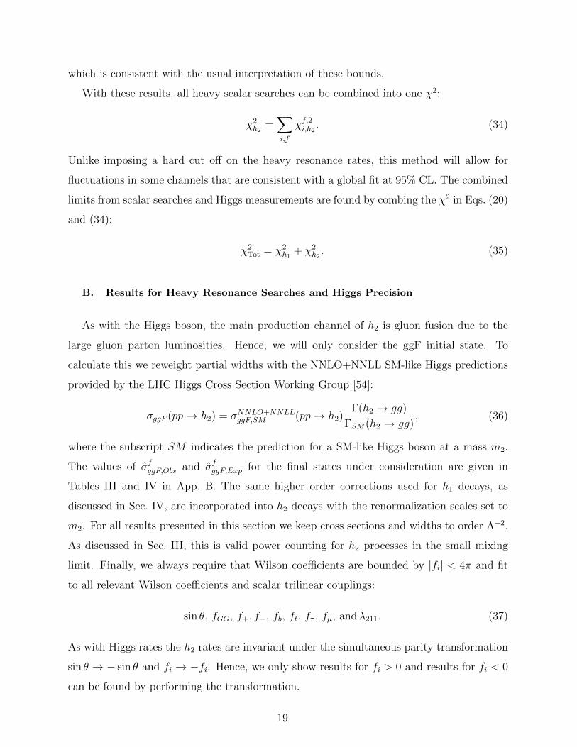
which is consistent with the usual interpretation of these bounds.
With these results, all heavy scalar searches can be combined into one χ2:
χ2h2
=∑i,f
χf,2i,h2 . (34)
Unlike imposing a hard cut off on the heavy resonance rates, this method will allow for
fluctuations in some channels that are consistent with a global fit at 95% CL. The combined
limits from scalar searches and Higgs measurements are found by combing the χ2 in Eqs. (20)
and (34):
χ2Tot = χ2
h1+ χ2
h2. (35)
B. Results for Heavy Resonance Searches and Higgs Precision
As with the Higgs boson, the main production channel of h2 is gluon fusion due to the
large gluon parton luminosities. Hence, we will only consider the ggF initial state. To
calculate this we reweight partial widths with the NNLO+NNLL SM-like Higgs predictions
provided by the LHC Higgs Cross Section Working Group [54]:
σggF (pp→ h2) = σNNLO+NNLLggF,SM (pp→ h2)
Γ(h2 → gg)
ΓSM(h2 → gg), (36)
where the subscript SM indicates the prediction for a SM-like Higgs boson at a mass m2.
The values of σfggF,Obs and σfggF,Exp for the final states under consideration are given in
Tables III and IV in App. B. The same higher order corrections used for h1 decays, as
discussed in Sec. IV, are incorporated into h2 decays with the renormalization scales set to
m2. For all results presented in this section we keep cross sections and widths to order Λ−2.
As discussed in Sec. III, this is valid power counting for h2 processes in the small mixing
limit. Finally, we always require that Wilson coefficients are bounded by |fi| < 4π and fit
to all relevant Wilson coefficients and scalar trilinear couplings:
sin θ, fGG, f+, f−, fb, ft, fτ , fµ, andλ211. (37)
As with Higgs rates the h2 rates are invariant under the simultaneous parity transformation
sin θ → − sin θ and fi → −fi. Hence, we only show results for fi > 0 and results for fi < 0
can be found by performing the transformation.
19
Page 20
0 1000 2000 3000 4000 5000|λ
211| (GeV)
-1
-0.75
-0.5
-0.25
0
0.25
0.5
0.75
1si
n θ
Higgs FitsHiggs Fits+Γ
2/m
2 < 0.1
Higgs+ScalarHiggs+Scalar+Γ
2/m
2 < 0.1
Scalar SearchScalar Search + Γ
2/m
2 < 0.1
m2 = 400 GeV
|fi| < 4π, Λ = 3 TeV
(a)
0 1000 2000 3000 4000 5000|λ
211| (GeV)
-1
-0.75
-0.5
-0.25
0
0.25
0.5
0.75
1
sin θ
Higgs FitsHiggs Fits+Γ
2/m
2 < 0.1
Higgs+ScalarHiggs+Scalar+Γ
2/m
2 < 0.1
Scalar SearchScalar Search + Γ
2/m
2 < 0.1
m2 = 600 GeV
|fi| < 4π, Λ = 3 TeV
(b)
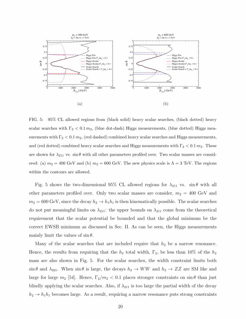
FIG. 5: 95% CL allowed regions from (black solid) heavy scalar searches, (black dotted) heavy
scalar searches with Γ2 < 0.1m2, (blue dot-dash) Higgs measurements, (blue dotted) Higgs mea-
surements with Γ2 < 0.1m2, (red dashed) combined heavy scalar searches and Higgs measurements,
and (red dotted) combined heavy scalar searches and Higgs measurements with Γ2 < 0.1m2. These
are shown for λ211 vs. sin θ with all other parameters profiled over. Two scalar masses are consid-
ered: (a) m2 = 400 GeV and (b) m2 = 600 GeV. The new physics scale is Λ = 3 TeV. The regions
within the contours are allowed.
Fig. 5 shows the two-dimensional 95% CL allowed regions for λ211 vs. sin θ with all
other parameters profiled over. Only two scalar masses are consider, m2 = 400 GeV and
m2 = 600 GeV, since the decay h2 → h1h1 is then kinematically possible. The scalar searches
do not put meaningful limits on λ211: the upper bounds on λ211 come from the theoretical
requirement that the scalar potential be bounded and that the global minimum be the
correct EWSB minimum as discussed in Sec. II. As can be seen, the Higgs measurements
mainly limit the values of sin θ.
Many of the scalar searches that are included require that h2 be a narrow resonance.
Hence, the results from requiring that the h2 total width, Γ2, be less than 10% of the h2
mass are also shown in Fig. 5. For the scalar searches, the width constraint limits both
sin θ and λ221. When sin θ is large, the decays h2 → WW and h2 → ZZ are SM like and
large for large m2 [54]. Hence, Γ2/m2 < 0.1 places stronger constraints on sin θ than just
blindly applying the scalar searches. Also, if λ211 is too large the partial width of the decay
h2 → h1h1 becomes large. As a result, requiring a narrow resonance puts strong constraints
20
Page 21
0 1 2 3 4
fGG
/Λ (TeV-1
)
-1
-0.75
-0.5
-0.25
0
0.25
0.5
0.75
1
sin θ
Higgs FitsHiggs+ScalarScalar SearchScalar Search + Γ
2/m
2 < 0.1
m2 = 200 GeV
|fi| < 4π, Λ = 3 TeV
(a)
0 1 2 3 4
fGG
/Λ (TeV-1
)
-1
-0.75
-0.5
-0.25
0
0.25
0.5
0.75
1
sin θ
Higgs FitsHiggs+ScalarScalar SearchScalar Search + Γ
2/m
2 < 0.1
m2 = 400 GeV
|fi| < 4π, Λ = 3 TeV
(b)
0 1 2 3 4
fGG
/Λ (TeV-1
)
-1
-0.75
-0.5
-0.25
0
0.25
0.5
0.75
1
sin θ
Higgs FitsHiggs+ScalarScalar SearchScalar Search + Γ
2/m
2 < 0.1
m2 = 600 GeV
|fi| < 4π, Λ = 3 TeV
(c)
0 1 2 3 4
ft/Λ (TeV
-1)
-1
-0.75
-0.5
-0.25
0
0.25
0.5
0.75
1
sin θ
Higgs FitsHiggs+ScalarScalar SearchScalar Search + Γ
2/m
2 < 0.1
m2 = 200 GeV
|fi| < 4π, Λ = 3 TeV
(d)
0 1 2 3 4
ft/Λ (TeV
-1)
-1
-0.75
-0.5
-0.25
0
0.25
0.5
0.75
1
sin θ
Higgs FitsHiggs+ScalarScalar SearchScalar Search
m2 = 400 GeV
|fi| < 4π, Λ = 3 TeV
+Γ2/m
2 < 0.1
(e)
0 1 2 3 4
ft/Λ (TeV
-1)
-1
-0.75
-0.5
-0.25
0
0.25
0.5
0.75
1
sin θ
Higgs FitsHiggs+ScalarScalar SearchScalar Search + Γ
2/m
2 < 0.1
m2 = 600 GeV
|fi| < 4π, Λ = 3 TeV
(f)
FIG. 6: 95% CL allowed regions from (black solid) heavy scalar searches, (black dotted) heavy
scalar searches with Γ2 < 0.1m2, (blue dot-dash) Higgs measurements, and (red dotted) combined
heavy scalar searches and Higgs measurements. The regions within the contours are allowed. These
are shown for (a,b,c) fGG and (d,e,f) ft vs. sin θ with all other parameters profiled over. Three
scalar masses are considered: (a,d) m2 = 200 GeV, (b,e) m2 = 400 GeV, and (c,f) m2 = 600 GeV.
The new physics scale is Λ = 3 TeV.
21
Page 22
on λ211. Higgs measurements already strongly constrain sin θ, so the effect of requiring a
narrow resonance limits the allowed values of λ211 for both Higgs measurements and their
combination with scalar searches.
The two-dimensional 95% CL allowed regions for fGG vs. sin θ and ft vs. sin θ with all
other parameters profiled over are shown in Fig. 63. As with the λ211 limits, requiring a
narrow width in the scalar search results squeezes the allowed parameter region for m2 = 400
and m2 = 600 GeV. The narrow width requirement does not significantly change the Higgs
precision and combination constraints. For the smaller m2, the narrow width requirement
makes no difference on any of the limits.
As can be seen in Fig. 6, Higgs measurements and scalar searches are complementary.
That is, the allowed regions for scalar searches and Higgs measurements do not fully overlap.
Indeed, the combined allowed region is smaller than the individual allowed regions. This is
particularly striking for m2 = 600 GeV.
Finally, in Fig. 7 we show the ∆χ2 distributions as a function sin θ for the BSM-EFT
and renormalizable model with all other parameters profiled over. In the BSM-EFT, the
shape of ∆χ2 changes dramatically. The 95% CL and 68% CL allowed regions also change
drastically and exactly how they change depends strongly on the h2 mass. It is clear that
even 3 TeV new physics effects can make a significant impact on the interpretation of current
measurements.
VII. CONCLUSION
A common assumption of simplified models at the LHC is that there are a few new
BSM particles that can be produced, while all other new particles are heavy and decoupled.
Under these assumptions, most studies of simplified models are renormalizable. However,
using EFT techniques it is possible to test the basic assumption that all other new particles
are indeed decoupled.
In this paper, we studied a popular simplified model, the real singlet extended SM, and
supplemented it with all possible dimension-5 operators involving the scalar singlet. We
studied the effects of the effective operators on the interpretation of Higgs signal strengths
3 The results for the remaining Wilson coefficients can be found in App. C
22
Page 23
(a) (b)
(c)
FIG. 7: ∆χ2 for combined Higgs measurements and scalar searches as a function of sin θ with
all other parameters profiled over. Both (black solid) Wilson coefficients with |fi| < 4π and
(blue dashed) fi = 0, i.e. dimension-5 terms set to zero. Three h2 masses are considered: (a)
m2 = 200 GeV, (b) m2 = 400 GeV, and (c) m2 = 600 GeV.
as well as searches for heavy new resonances. As we showed, even if the new physics occurs
at 3 TeV, the interpretation of these measurements and searches are changed drastically.
This study shows that even in the simplest of simplified model, the heavy new physics is not
“decoupled” even when the BSM-EFT expansion is valid. That is, it cannot be neglected
and the BSM-EFT should generically be considered.
In addition to the numerical results, we also gave a comprehensive discussion of the
counting in BSM-EFT for production and decay rates. We showed that while in the linear
23
Page 24
SMEFT power counting is relatively straightforward, power counting in a BSM-EFT is
strongly process and parameter space dependent. We also developed a new proposal to
consistently combine the limits from new resonance searches and precision measurements
via a χ2. This method allows for fluctuations in individual channels, while keeping the global
χ2 within allowable limits. This is unlike the usual cutoff method where all resonance cross
sections are strictly cut off at the observed limits [64].
Acknowledgments
We thank Jeong Han Kim, KC Kong, Tilman Plehn, Daniel Tapia Takaki, Yajuan Zheng,
for helpful discussions. Chris Rogan is thanked for reassuring IML that he is not crazy. IML
would like to thank the Institute for Theoretical Physics at Universitat Heidelberg for their
hospitality during the completion of this work. This work was performed in part at the
Aspen Center for Physics, which is supported by National Science Foundation grant PHY-
1607611. SA, IML, and MS are supported in part by United States Department of Energy
grant number de-sc0017988. SA and MS are also supported in part by the State of Kansas
EPSCoR grant program. The data to reproduce the plots has been uploaded with the arXiv
submission or is available upon request.
Appendix A: Feynman Rules
1. Trilinear Scalar Couplings
The trilinear scalar couplings are defined as
V (h1, h2) ⊃1
3!λ111h
31 +
1
2λ211h
21h2 +
1
2λ221h1h
22 +
1
3!λ222h
32. (A1)
where λ111 and λ211 are given in Sec. II, and
λ221 =m2
1 + 2m22
vcos θ sin2 θ + 2 b3 cos2 θ sin θ + a2v cos θ
(cos2 θ − 2 sin2 θ
)+
3 a3v2
2Λcos2 θ sin θ − a4v
2
Λsin θ
(2 cos2 θ − sin2 θ
)(A2)
λ222 = −3m22
vsin3 θ + 2 b3 cos3 θ − 3 a2v cos2 θ sin θ +
3 a3v2
2 Λcos3 θ (A3)
+3 a4v
2
Λcos θ sin2 θ
24
Page 25
2. hi − f − f and hi − V − V ′ couplings
The vertex rules, with all momenta outgoing, are
Vh1ff = −imf
v(cos θ +
f sfΛv sin θ) (A4)
Vh1gµ(p1)gν(p2) = −i g2s
4π2
f sGGΛ
sin θ(ηµνp1 · p2 − p1νp2µ) (A5)
Vh1γµ(p1)γν(p2) = −i e2
4π2
f sBB + f sWW
Λsin θ(ηµνp1 · p2 − p1νp2µ) (A6)
Vh1W+µ (p1)W
−ν (p2)
= 2im2w
vηµν cos θ − i g
2
4π2
f sWW
Λsin θ(ηµνp1 · p2 − p1νp2µ) (A7)
Vh1Zµ(p1)Zν(p2) = 2im2z
vηµν cos θ − i g
2z
4π2
f sZZΛ
sin θ(ηµνp1 · p2 − p1νp2µ) (A8)
Vh1Zµ(p1)γν(p2) = −i2gze4π2
f sZγΛ
sin θ(ηµνp1 · p2 − p1νp2µ) (A9)
Vh2ff = −imf
v(− sin θ +
f sfΛv cos θ) (A10)
Vh2gµ(p1)gν(p2) = −i g2s
4π2
f sGGΛ
cos θ(ηµνp1 · p2 − p1νp2µ) (A11)
Vh2γµ(p1)γν(p2) = −i e2
4π2
f sBB + f sWW
Λcos θ(ηµνp1 · p2 − p1νp2µ) (A12)
Vh2W+µ (p1)W
−ν (p2)
= −2im2w
vηµν sin θ − i g
2
4π2
f sWW
Λcos θ(ηµνp1 · p2 − p1νp2µ) (A13)
Vh2Zµ(p1)Zν(p2) = −2im2z
vηµν sin θ − i g
2z
4π2
f sZZΛ
cos θ(ηµνp1 · p2 − p1νp2µ) (A14)
Vh2Zµ(p1)γν(p2) = −i2gze4π2
f sZγΛ
cos θ(ηµνp1 · p2 − p1νp2µ) (A15)
with gz = gcos θw
, f sZZ = f sBB sin4 θw + f sWW cos4 θw, and f sZγ = f sBB sin2 θw + f sWW cos4 θw
Appendix B: Signal Strengths/Bounds
1. Higgs Signal Strengths
We now give the signal strengths used in our fits. These are chosen to be the measured
signal strengths with the most integrated luminosity in a given channel. All results are from
Run 2, with up to 139 fb−1 of accumulated data. The guide to non-obvious abbreviations:
ggF = gluon fusion, VBF = vector boson fusion, Wh1 = Higgs associated production with
a W , Zh1 = Higgs associated production with a Z, V h1 = combination of Wh1 and Zh1,
and V V ∗ = combination of ZZ∗ and WW ∗.
25
Page 26
γγ ZZ∗ WW ∗ V V ∗ ττ bb
ggF 0.96+0.14−0.14 [65] 0.98+0.11
−0.11 [66] 1.08+0.19−0.19 [65] * 0.96+0.59
−0.52 [65] *
VBF 1.39+0.40−0.35 [65] 1.4+0.52
−0.52 [66] 0.59+0.36−0.35 [65] * 1.16+0.58
−0.53 [65] 3.01+1.67−1.61 [65]
V h1 1.09+0.58−0.54 [65] 1.3+0.93
−0.93 [66] * * * 1.19+0.27−0.25 [65]
Wh1 * * 2.3+1.2−1.0 [67] * * *
Zh1 * * 2.9+1.9−1.3 [67] * * *
tth1 + th1 * * * 1.50+0.59−0.57 [65] 1.38+1.13
−0.96 [65] 0.79+0.60−0.59 [65]
tth1 1.38+0.41−0.36 [68] * * * * *
TABLE I: ATLAS Signal Strengths at 13 TeV. The asterisks indicates those signal strengths are
not used in our fits. The production modes are listed in the rows and the decay modes are listed
in the columns. Stars indicate signal strengths we do not include in our fits.
γγ ZZ∗ WW ∗ ττ bb
ggF 1.15+0.15−0.15 [69] 0.97+0.13
−0.11 [70] 1.35+0.21−0.19 [71] 0.36+0.36
−0.37 [72] 2.51+2.43−2.01 [71]
VBF 0.8+0.40−0.30 [69] 0.64+0.48
−0.37 [70] 0.28+0.64−0.60 [71] * *
VBF+V h1 * * * 1.03+0.30−0.29 [72] *
V h1 * 1.15+0.93−0.74 [70] * * 1.06+0.26
−0.26 [73]
Wh1 3.76+1.48−1.35 [71] * 3.91+2.26
−2.01 [71] * *
Zh1 0.00+1.14−0.00 [71] * 0.96+1.81
−1.46 [71] * *
tth1 + th1 * 0.13+0.93−0.13 [70] * * *
tth1 1.7+0.60−0.50 [74] * 1.6+0.65
−0.59 [71] * 1.15+0.32−0.29 [75]
TABLE II: CMS Signal Strengths at 13 TeV. The asterisks indicates those signal strengths are not
used in our fits. The production modes are listed in the rows and the decay modes are listed in
the columns. Stars indicate signal strengths we do not include in our fits.
2. Scalar Search Bounds
Now we give the relevant observed and expected scalar cross section upper bounds from
ATLAS in Tab. B 2 and CMS in Tab. B 2.
26
Page 27
σ(pb) m2 = 200 GeV m2 = 400 GeV m2 = 600 GeV
Obs. Exp. Obs. Exp. Obs. Exp.
pp→ h2 → Zγ * * 0.027 pb [76] 0.027 pb [76] 0.0081 pb [76] 0.0125 pb [76]
pp→ h2 → γγ 0.0216 pb [77] 0.0161 pb [77] 0.00275 pb [77] 0.00295 pb [77] 0.00187 pb [77] 0.00124 pb [77]
pp→ h2 → ZZ 0.36 pb [78] 0.32 pb [78] * * * *
pp→ h2 →WW 6.4 pb [79] 5.6 pb [79] * * * *
pp→ h2 →WW + ZZ * * 0.296 pb [80] 0.296 pb [80] 0.0456 pb [80] 0.0612 pb [80]
pp→ h2 → h1h1 → bbbb * * 0.222 pb [81] 0.210 pb [81] 0.0273 pb [81] 0.0391 pb [81]
pp→ h2 → h1h1 → bbγγ * * 0.00209 pb [82] 0.00176 pb [82] 7.11× 10⁻⁴ pb [82] 8.33× 10⁻⁴ pb [82]
pp→ h2 → h1h1 → bbτ+τ− * * 0.0397 pb [83] 0.0445 pb [83] 0.00907 pb [83] 0.0117 pb [83]
pp→ h2 → h1h1 → bbWW * * * * 0.301 pb [84] 0.319 pb [84]
pp→ h2 → h1h1 → γγWW * * 0.0090 pb [85] 0.00630 pb [85] * *
pp→ h2 → h1h1 →WWWW * * 0.242 pb [86] 0.309 pb [86] * *
pp→ h2 → τ+τ− 0.781 pb [87] 0.902 pb [87] 0.151 pb [87] 0.0960 pb [87] 0.0526 pb [87] 0.0349 pb [87]
pp→ h2 → µ+µ− 0.0442 pb [88] 0.0258 pb [88] 0.0074 pb [88] 0.0079 pb [88] 0.006 pb [88] 0.0041 pb [88]
pp→ h2 → jj * * * * 9.95 pb [89] 10.5 pb [89]
TABLE III: Observed (Obs.) and Expected (Exp) 95 % CL ATLAS upper limit on cross section
times branching ratio for heavy resonances at center of mass energy 13 TeV. Asterisks indicate
that either there were no relevant results or they were not included in the fit. Where needed, the
bounds on di-Higgs production were weighted by the SM Higgs branching ratios as provided by
the LHC Higgs Cross Section Working Group [54].
27
Page 28
σ(pb) m2 = 200 GeV m2 = 400 GeV m2 = 600 GeV
Obs. Exp. Obs. Exp. Obs. Exp.
pp→ h2 → Zγ * * 0.022 pb [90] 0.027 pb [90] 0.016 pb [90] 0.013 pb [90]
pp→ h2 → γγ * * * * 0.0014 [91] pb 0.0016 pb [91]
pp→ h2 → ZZ 0.24 pb [92] 0.33 pb [92] 0.067 pb [92] 0.083 pb [92] 0.025 pb [92] 0.032 pb [92]
pp→ h2 →WW 6.8 pb [93] 5.9 pb [93] 1.0 pb [93] 1.21 pb [93] 0.43 pb [93] 0.33 pb [93]
pp→ h2 → h1h1 → bbbb * * 0.163 pb [94] 0.179 pb [94] 0.0355 pb [94] 0.0396 pb [94]
pp→ h2 → h1h1 → bbγγ * * 0.0012 pb [95] 0.0012 pb [95] 4.4× 10⁻⁴ pb [95] 4.4× 10⁻⁴ pb [95]
pp→ h2 → h1h1 → bbτ+τ− * * 0.0860 pb [96] 0.106 pb [96] 0.0314 pb [96] 0.0200 pb [96]
pp→ h2 → h1h1 → bbZZ * * 0.52 pb [97] 0.70 pb [97] 0.16 pb [97] 0.31 pb [97]
pp→ h2 → τ+τ− 0.823 pb [98] 0.887 pb [98] 0.0743 pb [98] 0.0851 pb [98] 0.0495 pb [98] 0.0294 pb [98]
pp→ h2 → µ+µ− 0.0175 pb [99] 0.0112 pb [99] 0.0028 pb [99] 0.003 pb [99] 0.00175 pb [99] 0.00175 pb [99]
pp→ h2 → dijets(gg) * * * * 71.8 pb [100] 38.4 pb [100]
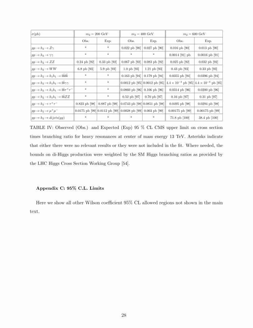
TABLE IV: Observed (Obs.) and Expected (Exp) 95 % CL CMS upper limit on cross section
times branching ratio for heavy resonances at center of mass energy 13 TeV. Asterisks indicate
that either there were no relevant results or they were not included in the fit. Where needed, the
bounds on di-Higgs production were weighted by the SM Higgs branching ratios as provided by
the LHC Higgs Cross Section Working Group [54].
Appendix C: 95% C.L. Limits
Here we show all other Wilson coefficient 95% CL allowed regions not shown in the main
text.
28
Page 29
0 1 2 3 4
fb/Λ (TeV
-1)
-1
-0.75
-0.5
-0.25
0
0.25
0.5
0.75
1
sin θ
Higgs FitsHiggs+ScalarScalar SearchScalar Search + Γ
2/m
2 < 0.1
m2 = 200 GeV
|fi| < 4π, Λ = 3 TeV
(a)
0 1 2 3 4
fb/Λ (TeV
-1)
-1
-0.75
-0.5
-0.25
0
0.25
0.5
0.75
1
sin θ
Higgs FitsHiggs+ScalarScalar SearchScalar Search + Γ
2/m
2 < 0.1
m2 = 400 GeV
|fi| < 4π, Λ = 3 TeV
(b)
0 1 2 3 4
fb/Λ (TeV
-1)
-1
-0.75
-0.5
-0.25
0
0.25
0.5
0.75
1
sin θ
Higgs FitsHiggs+ScalarScalar SearchScalar Search + Γ
2/m
2 < 0.1
m2 = 600 GeV
|fi| < 4π, Λ = 3 TeV
(c)
0 1 2 3 4
fτ/Λ (TeV-1
)
-1
-0.75
-0.5
-0.25
0
0.25
0.5
0.75
1
sin θ
Higgs FitsHiggs+ScalarScalar SearchScalar Search + Γ
2/m
2 < 0.1
m2 = 200 GeV
|fi| < 4π, Λ = 3 TeV
(d)
0 1 2 3 4
fτ/Λ (TeV-1
)
-1
-0.75
-0.5
-0.25
0
0.25
0.5
0.75
1
sin θ
Higgs FitsHiggs+ScalarScalar SearchScalar Search + Γ
2/m
2 < 0.1
m2 = 400 GeV
|fi| < 4π, Λ = 3 TeV
(e)
0 1 2 3 4
fτ/Λ (TeV-1
)
-1
-0.75
-0.5
-0.25
0
0.25
0.5
0.75
1
sin θ
Higgs FitsHiggs+ScalarScalar SearchScalar Search + Γ
2/m
2 < 0.1
m2 = 600 GeV
|fi| < 4π, Λ = 3 TeV
(f)
FIG. 8: Same as Fig. 6 for (a,b,c) fband (d,e,f) fτ vs. sin θ with all other parameters profiled
over. Three scalar masses are considered: (a,d) m2 = 200 GeV, (b,e) m2 = 400 GeV, and (c,f)
m2 = 600 GeV. The new physics scale is Λ = 3 TeV.
29
Page 30
0 1 2 3 4
f-/Λ (TeV
-1)
-1
-0.75
-0.5
-0.25
0
0.25
0.5
0.75
1
sin θ
Higgs FitsHiggs+ScalarScalar SearchScalar Search + Γ
2/m
2 < 0.1
m2 = 200 GeV
|fi| < 4π, Λ = 3 TeV
(a)
0 1 2 3 4
f-/Λ (TeV
-1)
-1
-0.75
-0.5
-0.25
0
0.25
0.5
0.75
1
sin θ
Higgs FitsHiggs+ScalarScalar SearchScalar Search + Γ
2/m
2 < 0.1
m2 = 400 GeV
|fi| < 4π, Λ = 3 TeV
(b)
0 1 2 3 4
f-/Λ (TeV
-1)
-1
-0.75
-0.5
-0.25
0
0.25
0.5
0.75
1
sin θ
Higgs FitsHiggs+ScalarScalar SearchScalar Search + Γ
2/m
2 < 0.1
m2 = 600 GeV
|fi| < 4π, Λ = 3 TeV
(c)
0 1 2 3 4
f+/Λ (TeV
-1)
-1
-0.75
-0.5
-0.25
0
0.25
0.5
0.75
1
sin θ
Higgs FitsHiggs+ScalarScalar SearchScalar Search + Γ
2/m
2 < 0.1
m2 = 200 GeV
|fi| < 4π, Λ = 3 TeV
(d)
0 1 2 3 4
f+/Λ (TeV
-1)
-1
-0.75
-0.5
-0.25
0
0.25
0.5
0.75
1
sin θ
Higgs FitsHiggs+ScalarScalar SearchScalar Search + Γ
2/m
2 < 0.1
m2 = 400 GeV
|fi| < 4π, Λ = 3 TeV
(e)
0 1 2 3 4
f+/Λ (TeV
-1)
-1
-0.75
-0.5
-0.25
0
0.25
0.5
0.75
1
sin θ
Higgs FitsHiggs+ScalarScalar SearchScalar Search + Γ
2/m
2 < 0.1
m2 = 600 GeV
|fi| < 4π, Λ = 3 TeV
(f)
FIG. 9: Same as Fig. 6 for (a,b,c) f−and (d,e,f) f+ vs. sin θ with all other parameters profiled
over. Three scalar masses are considered: (a,d) m2 = 200 GeV, (b,e) m2 = 400 GeV, and (c,f)
m2 = 600 GeV. The new physics scale is Λ = 3 TeV.
30
Page 31
0 1 2 3 4
fµ/Λ (TeV-1
)
-1
-0.75
-0.5
-0.25
0
0.25
0.5
0.75
1
sin θ
Higgs FitsHiggs+ScalarScalar SearchScalar Search + Γ
2/m
2 < 0.1
m2 = 200 GeV
|fi| < 4π, Λ = 3 TeV
(a)
0 1 2 3 4
fµ/Λ (TeV-1
)
-1
-0.75
-0.5
-0.25
0
0.25
0.5
0.75
1
sin θ
Higgs FitsHiggs+ScalarScalar SearchScalar Search + Γ
2/m
2 < 0.1
m2 = 400 GeV
|fi| < 4π, Λ = 3 TeV
(b)
0 1 2 3 4
fµ/Λ (TeV-1
)
-1
-0.75
-0.5
-0.25
0
0.25
0.5
0.75
1
sin θ
Higgs FitsHiggs+ScalarScalar SearchScalar Search + Γ
2/m
2 < 0.1
m2 = 600 GeV
|fi| < 4π, Λ = 3 TeV
(c)
FIG. 10: Same as Fig. 6 for fµ vs. sin θ with all other parameters profiled over. Three scalar
masses are considered: (a,d) m2 = 200 GeV, (b,e) m2 = 400 GeV, and (c,f) m2 = 600 GeV. The
new physics scale is Λ = 3 TeV.
31
Page 32
[1] D. Alves, , LHC New Physics Working Group Collaboration, Simplified Models for
LHC New Physics Searches, J. Phys. G39 (2012) 105005, arXiv:1105.2838 [hep-ph].
[2] J. H. Kim and I. M. Lewis, Loop Induced Single Top Partner Production and Decay at the
LHC, JHEP 05 (2018) 095, arXiv:1803.06351 [hep-ph].
[3] H. Alhazmi, J. H. Kim, K. Kong, and I. M. Lewis, Shedding Light on Top Partner at the
LHC, JHEP 01 (2019) 139, arXiv:1808.03649 [hep-ph].
[4] J. C. Criado and M. Perez-Victoria, Vector-like quarks with non-renormalizable
interactions, JHEP 01 (2020) 057, arXiv:1908.08964 [hep-ph].
[5] W. Buchmuller and D. Wyler, Effective Lagrangian Analysis of New Interactions and
Flavor Conservation, Nucl. Phys. B268 (1986) 621–653.
[6] B. Grzadkowski, M. Iskrzynski, M. Misiak, and J. Rosiek, Dimension-Six Terms in the
Standard Model Lagrangian, JHEP 10 (2010) 085, arXiv:1008.4884 [hep-ph].
[7] I. Brivio and M. Trott, The Standard Model as an Effective Field Theory, Phys. Rept. 793
(2019) 1–98, arXiv:1706.08945 [hep-ph].
[8] S. Dawson and I. M. Lewis, Singlet Model Interference Effects with High Scale UV Physics,
Phys. Rev. D95 no. 1, (2017) 015004, arXiv:1605.04944 [hep-ph].
[9] M. Bauer, A. Butter, J. Gonzalez-Fraile, T. Plehn, and M. Rauch, Learning from a
Higgs-like scalar resonance, Phys. Rev. D95 no. 5, (2017) 055011, arXiv:1607.04562
[hep-ph].
[10] Anisha, S. Das Bakshi, J. Chakrabortty, and S. Prakash, Hilbert Series and Plethystics:
Paving the path towards 2HDM- and MLRSM-EFT, JHEP 09 (2019) 035,
arXiv:1905.11047 [hep-ph].
[11] S. Karmakar and S. Rakshit, Relaxed constraints on the heavy scalar masses in 2HDM,
Phys. Rev. D100 no. 5, (2019) 055016, arXiv:1901.11361 [hep-ph].
[12] A. Crivellin, M. Ghezzi, and M. Procura, Effective Field Theory with Two Higgs Doublets,
JHEP 09 (2016) 160, arXiv:1608.00975 [hep-ph].
[13] J. L. Diaz-Cruz, J. Hernandez-Sanchez, and J. J. Toscano, An Effective Lagrangian
description of charged Higgs decays H+ →W+γ, W+Z and W+ h0, Phys. Lett. B512
(2001) 339–348, arXiv:hep-ph/0106001 [hep-ph].
32
Page 33
[14] S. Bar-Shalom, J. Cohen, A. Soni, and J. Wudka, Phenomenology of TeV-scale scalar
Leptoquarks in the EFT, Phys. Rev. D100 no. 5, (2019) 055020, arXiv:1812.03178
[hep-ph].
[15] M. Chala, G. Durieux, C. Grojean, L. de Lima, and O. Matsedonskyi, Minimally extended
SILH, JHEP 06 (2017) 088, arXiv:1703.10624 [hep-ph].
[16] D. O’Connell, M. J. Ramsey-Musolf, and M. B. Wise, Minimal Extension of the Standard
Model Scalar Sector, Phys. Rev. D75 (2007) 037701, arXiv:hep-ph/0611014 [hep-ph].
[17] V. Barger, P. Langacker, M. McCaskey, M. J. Ramsey-Musolf, and G. Shaughnessy, LHC
Phenomenology of an Extended Standard Model with a Real Scalar Singlet, Phys. Rev. D77
(2008) 035005, arXiv:0706.4311 [hep-ph].
[18] M. Bowen, Y. Cui, and J. D. Wells, Narrow trans-TeV Higgs bosons and H → hh decays:
Two LHC search paths for a hidden sector Higgs boson, JHEP 03 (2007) 036,
arXiv:hep-ph/0701035 [hep-ph].
[19] J. Choi and R. R. Volkas, Real Higgs singlet and the electroweak phase transition in the
Standard Model, Phys. Lett. B317 (1993) 385–391, arXiv:hep-ph/9308234 [hep-ph].
[20] S. Profumo, M. J. Ramsey-Musolf, and G. Shaughnessy, Singlet Higgs phenomenology and
the electroweak phase transition, JHEP 08 (2007) 010, arXiv:0705.2425 [hep-ph].
[21] J. R. Espinosa, T. Konstandin, and F. Riva, Strong Electroweak Phase Transitions in the
Standard Model with a Singlet, Nucl. Phys. B854 (2012) 592–630, arXiv:1107.5441
[hep-ph].
[22] D. Curtin, P. Meade, and C.-T. Yu, Testing Electroweak Baryogenesis with Future
Colliders, JHEP 11 (2014) 127, arXiv:1409.0005 [hep-ph].
[23] C.-Y. Chen, J. Kozaczuk, and I. M. Lewis, Non-resonant Collider Signatures of a
Singlet-Driven Electroweak Phase Transition, JHEP 08 (2017) 096, arXiv:1704.05844
[hep-ph].
[24] M.-L. Xiao and J.-H. Yu, Electroweak baryogenesis in a scalar-assisted vectorlike fermion
model, Phys. Rev. D94 no. 1, (2016) 015011, arXiv:1509.02931 [hep-ph].
[25] J. M. Cline, Is electroweak baryogenesis dead?, Phil. Trans. Roy. Soc. Lond. A376
no. 2114, (2018) 20170116, arXiv:1704.08911 [hep-ph]. [,339(2017)].
[26] W. Chao, CP Violation at the Finite Temperature, Phys. Lett. B796 (2019) 102–106,
arXiv:1706.01041 [hep-ph].
33
Page 34
[27] N. F. Bell, M. J. Dolan, L. S. Friedrich, M. J. Ramsey-Musolf, and R. R. Volkas,
Electroweak Baryogenesis with Vector-like Leptons and Scalar Singlets, JHEP 09 (2019)
012, arXiv:1903.11255 [hep-ph].
[28] J. R. Espinosa, B. Gripaios, T. Konstandin, and F. Riva, Electroweak Baryogenesis in
Non-minimal Composite Higgs Models, JCAP 1201 (2012) 012, arXiv:1110.2876
[hep-ph].
[29] J. M. Cline and K. Kainulainen, Electroweak baryogenesis and dark matter from a singlet
Higgs, JCAP 1301 (2013) 012, arXiv:1210.4196 [hep-ph].
[30] F. P. Huang, Z. Qian, and M. Zhang, Exploring dynamical CP violation induced
baryogenesis by gravitational waves and colliders, Phys. Rev. D98 no. 1, (2018) 015014,
arXiv:1804.06813 [hep-ph].
[31] T. Robens and T. Stefaniak, Status of the Higgs Singlet Extension of the Standard Model
after LHC Run 1, Eur. Phys. J. C75 (2015) 104, arXiv:1501.02234 [hep-ph].
[32] D. Buttazzo, F. Sala, and A. Tesi, Singlet-like Higgs bosons at present and future colliders,
JHEP 11 (2015) 158, arXiv:1505.05488 [hep-ph].
[33] T. Robens and T. Stefaniak, LHC Benchmark Scenarios for the Real Higgs Singlet
Extension of the Standard Model, Eur. Phys. J. C76 no. 5, (2016) 268, arXiv:1601.07880
[hep-ph].
[34] I. M. Lewis and M. Sullivan, Benchmarks for Double Higgs Production in the Singlet
Extended Standard Model at the LHC, Phys. Rev. D96 no. 3, (2017) 035037,
arXiv:1701.08774 [hep-ph].
[35] A. Ilnicka, T. Robens, and T. Stefaniak, Constraining Extended Scalar Sectors at the LHC
and beyond, Mod. Phys. Lett. A33 no. 10n11, (2018) 1830007, arXiv:1803.03594
[hep-ph].
[36] S. Weinberg, Baryon and Lepton Nonconserving Processes, Phys. Rev. Lett. 43 (1979)
1566–1570.
[37] C.-Y. Chen, S. Dawson, and I. M. Lewis, Exploring resonant di-Higgs boson production in
the Higgs singlet model, Phys. Rev. D91 no. 3, (2015) 035015, arXiv:1410.5488 [hep-ph].
[38] C. Degrande, N. Greiner, W. Kilian, O. Mattelaer, H. Mebane, T. Stelzer, S. Willenbrock,
and C. Zhang, Effective Field Theory: A Modern Approach to Anomalous Couplings,
Annals Phys. 335 (2013) 21–32, arXiv:1205.4231 [hep-ph].
34
Page 35
[39] L. Lehman, Extending the Standard Model Effective Field Theory with the Complete Set of
Dimension-7 Operators, Phys. Rev. D90 no. 12, (2014) 125023, arXiv:1410.4193
[hep-ph].
[40] B. Henning, X. Lu, T. Melia, and H. Murayama, 2, 84, 30, 993, 560, 15456, 11962,
261485, ...: Higher dimension operators in the SM EFT, JHEP 08 (2017) 016,
arXiv:1512.03433 [hep-ph]. [Erratum: JHEP09,019(2019)].
[41] A. Kobach, Baryon Number, Lepton Number, and Operator Dimension in the Standard
Model, Phys. Lett. B758 (2016) 455–457, arXiv:1604.05726 [hep-ph].
[42] S. G. Gorishnii, A. L. Kataev, S. A. Larin, and L. R. Surguladze, Corrected Three Loop
QCD Correction to the Correlator of the Quark Scalar Currents and γ (Tot) (H0 →
Hadrons), Mod. Phys. Lett. A5 (1990) 2703–2712.
[43] K. G. Chetyrkin, Correlator of the quark scalar currents and Gamma(tot) (H —¿ hadrons)
at O (alpha-s**3) in pQCD, Phys. Lett. B390 (1997) 309–317, arXiv:hep-ph/9608318
[hep-ph].
[44] K. G. Chetyrkin, B. A. Kniehl, and M. Steinhauser, Three loop O (alpha-s**2 G(F)
M(t)**2) corrections to hadronic Higgs decays, Nucl. Phys. B490 (1997) 19–39,
arXiv:hep-ph/9701277 [hep-ph].
[45] K. G. Chetyrkin and M. Steinhauser, Complete QCD corrections of order O (alpha-s**3) to
the hadronic Higgs decay, Phys. Lett. B408 (1997) 320–324, arXiv:hep-ph/9706462
[hep-ph].
[46] A. Djouadi, The Anatomy of electro-weak symmetry breaking. I: The Higgs boson in the
standard model, Phys. Rept. 457 (2008) 1–216, arXiv:hep-ph/0503172 [hep-ph].
[47] A. Djouadi, M. Spira, and P. M. Zerwas, Production of Higgs bosons in proton colliders:
QCD corrections, Phys. Lett. B264 (1991) 440–446.
[48] S. Dawson, Radiative corrections to Higgs boson production, Nucl. Phys. B359 (1991)
283–300.
[49] H.-Q. Zheng and D.-D. Wu, First order QCD corrections to the decay of the Higgs boson
into two photons, Phys. Rev. D42 (1990) 3760–3763.
[50] A. Djouadi, M. Spira, J. J. van der Bij, and P. M. Zerwas, QCD corrections to gamma
gamma decays of Higgs particles in the intermediate mass range, Phys. Lett. B257 (1991)
187–190.
35
Page 36
[51] S. Dawson and R. P. Kauffman, QCD corrections to H —¿ gamma gamma, Phys. Rev. D47
(1993) 1264–1267.
[52] K. Melnikov and O. I. Yakovlev, Higgs —¿ two photon decay: QCD radiative correction,
Phys. Lett. B312 (1993) 179–183, arXiv:hep-ph/9302281 [hep-ph].
[53] M. Spira, A. Djouadi, and P. M. Zerwas, QCD corrections to the H Z gamma coupling,
Phys. Lett. B276 (1992) 350–353.
[54] LHC Higgs Cross Section Working Group Collaboration, D. de Florian et al., ,
Handbook of LHC Higgs Cross Sections: 4. Deciphering the Nature of the Higgs Sector.
CERN Yellow Reports: Monographs. Oct, 2016. arXiv:1610.07922 [hep-ph].
[55] J. Alwall, R. Frederix, S. Frixione, V. Hirschi, F. Maltoni, O. Mattelaer, H. S. Shao,
T. Stelzer, P. Torrielli, and M. Zaro, The automated computation of tree-level and
next-to-leading order differential cross sections, and their matching to parton shower
simulations, JHEP 07 (2014) 079, arXiv:1405.0301 [hep-ph].
[56] A. Alloul, N. D. Christensen, C. Degrande, C. Duhr, and B. Fuks, FeynRules 2.0 - A
complete toolbox for tree-level phenomenology, Comput. Phys. Commun. 185 (2014)
2250–2300, arXiv:1310.1921 [hep-ph].
[57] R. D. Ball et al., Parton distributions with LHC data, Nucl. Phys. B867 (2013) 244–289,
arXiv:1207.1303 [hep-ph].
[58] P. Azzi et al., Report from Working Group 1: Standard Model Physics at the HL-LHC and
HE-LHC, CERN Yellow Rep. Monogr. 7 (2019) 1–220, arXiv:1902.04070 [hep-ph].
[59] J. Baglio, S. Dawson, and I. M. Lewis, An NLO QCD effective field theory analysis of
W+W− production at the LHC including fermionic operators, Phys. Rev. D96 no. 7,
(2017) 073003, arXiv:1708.03332 [hep-ph].
[60] J. Baglio, S. Dawson, and I. M. Lewis, NLO effects in EFT fits to W+W− production at
the LHC, Phys. Rev. D99 no. 3, (2019) 035029, arXiv:1812.00214 [hep-ph].
[61] J. Baglio, S. Dawson, and S. Homiller, QCD corrections in Standard Model EFT fits to WZ
and WW production, Phys. Rev. D100 no. 11, (2019) 113010, arXiv:1909.11576
[hep-ph].
[62] J. Baglio, S. Dawson, S. Homiller, S. D. Lane, and I. M. Lewis, Validity of SMEFT studies
of VH and VV Production at NLO, arXiv:2003.07862 [hep-ph].
[63] T. Corbett, O. J. P. Eboli, D. Goncalves, J. Gonzalez-Fraile, T. Plehn, and M. Rauch, The
36
Page 37
Higgs Legacy of the LHC Run I, JHEP 08 (2015) 156, arXiv:1505.05516 [hep-ph].
[64] P. Bechtle, S. Heinemeyer, O. Stol, T. Stefaniak, and G. Weiglein, HiggsSignals:
Confronting arbitrary Higgs sectors with measurements at the Tevatron and the LHC, Eur.
Phys. J. C74 no. 2, (2014) 2711, arXiv:1305.1933 [hep-ph].
[65] G. Aad et al., , ATLAS Collaboration, Combined measurements of Higgs boson production
and decay using up to 80 fb−1 of proton-proton collision data at√s = 13 TeV collected with
the ATLAS experiment, Phys. Rev. D101 no. 1, (2020) 012002, arXiv:1909.02845
[hep-ex].
[66] ATLAS Collaboration Collaboration, Measurements of the Higgs boson inclusive,
differential and production cross sections in the 4` decay channel at√s = 13 TeV with the
ATLAS detector, Tech. Rep. ATLAS-CONF-2019-025, CERN, Geneva, Jul, 2019.
[67] G. Aad et al., , ATLAS Collaboration, Measurement of the production cross section for a
Higgs boson in association with a vector boson in the H →WW ∗ → `ν`ν channel in pp
collisions at√s = 13 TeV with the ATLAS detector, Phys. Lett. B798 (2019) 134949,
arXiv:1903.10052 [hep-ex].
[68] ATLAS Collaboration Collaboration, Measurement of Higgs boson production in
association with a tt pair in the diphoton decay channel using 139 fb−1 of LHC data
collected at√s = 13 TeV by the ATLAS experiment, Tech. Rep. ATLAS-CONF-2019-004,
CERN, Geneva, Mar, 2019.
[69] CMS Collaboration Collaboration, Measurements of Higgs boson production via gluon
fusion and vector boson fusion in the diphoton decay channel at√s = 13 TeV, Tech. Rep.
CMS-PAS-HIG-18-029, CERN, Geneva, 2019.
[70] CMS Collaboration Collaboration, Measurements of properties of the Higgs boson in the
four-lepton final state in proton-proton collisions at√s = 13 TeV, Tech. Rep.
CMS-PAS-HIG-19-001, CERN, Geneva, 2019.
[71] A. M. Sirunyan et al., , CMS Collaboration, Combined measurements of Higgs boson
couplings in proton–proton collisions at√s = 13 TeV, Eur. Phys. J. C79 no. 5, (2019) 421,
arXiv:1809.10733 [hep-ex].
[72] CMS Collaboration Collaboration, Measurement of Higgs boson production and decay to
the ττ final state, Tech. Rep. CMS-PAS-HIG-18-032, CERN, Geneva, 2019.
[73] A. M. Sirunyan et al., , CMS Collaboration, Observation of Higgs boson decay to bottom
37
Page 38
quarks, Phys. Rev. Lett. 121 no. 12, (2018) 121801, arXiv:1808.08242 [hep-ex].
[74] CMS Collaboration Collaboration, Measurement of the associated production of a Higgs
boson and a pair of top-antitop quarks with the Higgs boson decaying to two photons in
proton-proton collisions at√s = 13 TeV, Tech. Rep. CMS-PAS-HIG-18-018, CERN,
Geneva, 2018.
[75] CMS Collaboration Collaboration, Measurement of ttH production in the H→ bb decay
channel in 41.5 fb−1 of proton-proton collision data at√s = 13 TeV, Tech. Rep.
CMS-PAS-HIG-18-030, CERN, Geneva, 2019.
[76] M. Aaboud et al., , ATLAS Collaboration, Searches for the Zγ decay mode of the Higgs
boson and for new high-mass resonances in pp collisions at√s = 13 TeV with the ATLAS
detector, JHEP 10 (2017) 112, arXiv:1708.00212 [hep-ex].
[77] M. Aaboud et al., , ATLAS Collaboration, Search for new phenomena in high-mass
diphoton final states using 37 fb−1 of proton–proton collisions collected at√s = 13 TeV
with the ATLAS detector, Phys. Lett. B775 (2017) 105–125, arXiv:1707.04147 [hep-ex].
[78] M. Aaboud et al., , ATLAS Collaboration, Search for heavy ZZ resonances in the
`+`−`+`− and `+`−νν final states using proton–proton collisions at√s = 13 TeV with the
ATLAS detector, Eur. Phys. J. C78 no. 4, (2018) 293, arXiv:1712.06386 [hep-ex].
[79] M. Aaboud et al., , ATLAS Collaboration, Search for heavy resonances decaying into WW
in the eνµν final state in pp collisions at√s = 13 TeV with the ATLAS detector, Eur.
Phys. J. C78 no. 1, (2018) 24, arXiv:1710.01123 [hep-ex].
[80] M. Aaboud et al., , ATLAS Collaboration, Combination of searches for heavy resonances
decaying into bosonic and leptonic final states using 36 fb−1 of proton-proton collision data
at√s = 13 TeV with the ATLAS detector, Phys. Rev. D98 no. 5, (2018) 052008,
arXiv:1808.02380 [hep-ex].
[81] M. Aaboud et al., , ATLAS Collaboration, Search for pair production of Higgs bosons in
the bbbb final state using proton-proton collisions at√s = 13 TeV with the ATLAS detector,
JHEP 01 (2019) 030, arXiv:1804.06174 [hep-ex].
[82] M. Aaboud et al., , ATLAS Collaboration, Search for Higgs boson pair production in the
γγbb final state with 13 TeV pp collision data collected by the ATLAS experiment, JHEP 11
(2018) 040, arXiv:1807.04873 [hep-ex].
[83] M. Aaboud et al., , ATLAS Collaboration, Search for resonant and non-resonant Higgs
38
Page 39
boson pair production in the bbτ+τ− decay channel in pp collisions at√s = 13 TeV with
the ATLAS detector, Phys. Rev. Lett. 121 no. 19, (2018) 191801, arXiv:1808.00336
[hep-ex]. [Erratum: Phys. Rev. Lett.122,no.8,089901(2019)].
[84] M. Aaboud et al., , ATLAS Collaboration, Search for Higgs boson pair production in the
bbWW ∗ decay mode at√s = 13 TeV with the ATLAS detector, JHEP 04 (2019) 092,
arXiv:1811.04671 [hep-ex].
[85] M. Aaboud et al., , ATLAS Collaboration, Search for Higgs boson pair production in the
γγWW ∗ channel using pp collision data recorded at√s = 13 TeV with the ATLAS
detector, Eur. Phys. J. C78 no. 12, (2018) 1007, arXiv:1807.08567 [hep-ex].
[86] M. Aaboud et al., , ATLAS Collaboration, Search for Higgs boson pair production in the
WW (∗)WW (∗) decay channel using ATLAS data recorded at√s = 13 TeV, JHEP 05
(2019) 124, arXiv:1811.11028 [hep-ex].
[87] M. Aaboud et al., , ATLAS Collaboration, Search for additional heavy neutral Higgs and
gauge bosons in the ditau final state produced in 36 fb−1 of pp collisions at√s = 13 TeV
with the ATLAS detector, JHEP 01 (2018) 055, arXiv:1709.07242 [hep-ex].
[88] M. Aaboud et al., , ATLAS Collaboration, Search for scalar resonances decaying into
µ+µ− in events with and without b-tagged jets produced in proton-proton collisions at
√s = 13 TeV with the ATLAS detector, JHEP 07 (2019) 117, arXiv:1901.08144
[hep-ex].
[89] M. Aaboud et al., , ATLAS Collaboration, Search for low-mass dijet resonances using
trigger-level jets with the ATLAS detector in pp collisions at√s = 13 TeV, Phys. Rev. Lett.
121 no. 8, (2018) 081801, arXiv:1804.03496 [hep-ex].
[90] A. M. Sirunyan et al., , CMS Collaboration, Search for Zγ resonances using leptonic and
hadronic final states in proton-proton collisions at√s = 13 TeV, JHEP 09 (2018) 148,
arXiv:1712.03143 [hep-ex].
[91] A. M. Sirunyan et al., , CMS Collaboration, Search for physics beyond the standard model
in high-mass diphoton events from proton-proton collisions at√s = 13 TeV, Phys. Rev.
D98 no. 9, (2018) 092001, arXiv:1809.00327 [hep-ex].
[92] A. M. Sirunyan et al., , CMS Collaboration, Search for a new scalar resonance decaying to
a pair of Z bosons in proton-proton collisions at√s = 13 TeV, JHEP 06 (2018) 127,
arXiv:1804.01939 [hep-ex]. [Erratum: JHEP03,128(2019)].
39
Page 40
[93] A. M. Sirunyan et al., , CMS Collaboration, Search for a heavy Higgs boson decaying to a
pair of W bosons in proton-proton collisions at√s = 13 TeV, JHEP 03 (2020) 034,
arXiv:1912.01594 [hep-ex].
[94] A. M. Sirunyan et al., , CMS Collaboration, Search for resonant pair production of Higgs
bosons decaying to bottom quark-antiquark pairs in proton-proton collisions at 13 TeV,
JHEP 08 (2018) 152, arXiv:1806.03548 [hep-ex].
[95] A. M. Sirunyan et al., , CMS Collaboration, Search for Higgs boson pair production in the
γγbb final state in pp collisions at√s = 13 TeV, Phys. Lett. B788 (2019) 7–36,
arXiv:1806.00408 [hep-ex].
[96] A. M. Sirunyan et al., , CMS Collaboration, Search for Higgs boson pair production in
events with two bottom quarks and two tau leptons in proton–proton collisions at√s
=13TeV, Phys. Lett. B778 (2018) 101–127, arXiv:1707.02909 [hep-ex].
[97] CMS Collaboration Collaboration, Search for the resonant production of a pair of Higgs
bosons decaying to the bb-barZZ final state, Tech. Rep. CMS-PAS-HIG-18-013, CERN,
Geneva, 2019.
[98] A. M. Sirunyan et al., , CMS Collaboration, Search for additional neutral MSSM Higgs
bosons in the ττ final state in proton-proton collisions at√s = 13 TeV, JHEP 09 (2018)
007, arXiv:1803.06553 [hep-ex].
[99] A. M. Sirunyan et al., , CMS Collaboration, Search for MSSM Higgs bosons decaying to
µ+µ− in proton-proton collisions at√s = 13 TeV, Phys. Lett. B798 (2019) 134992,
arXiv:1907.03152 [hep-ex].
[100] A. M. Sirunyan et al., , CMS Collaboration, Search for narrow and broad dijet resonances
in proton-proton collisions at√s = 13 TeV and constraints on dark matter mediators and
other new particles, JHEP 08 (2018) 130, arXiv:1806.00843 [hep-ex].
40