Shift-Share Designs: Theory and Inference*

Rodrigo Adão† Michal Kolesár‡ Eduardo Morales§

August 13, 2018

Abstract

We study inference in shift-share regression designs, such as when a regional outcome is re-gressed on a weighted average of observed sectoral shocks, using regional sector shares as weights.We conduct a placebo exercise in which we estimate the effect of a shift-share regressor constructedwith randomly generated sectoral shocks on actual labor market outcomes across U.S. CommutingZones. Tests based on commonly used standard errors with 5% nominal significance level reject thenull of no effect in up to 55% of the placebo samples. We use a stylized economic model to showthat this overrejection problem arises because regression residuals are correlated across regionswith similar sectoral shares, independently of their geographic location. We derive novel inferencemethods that are valid under arbitrary cross-regional correlation in the regression residuals. Weshow that our methods yield substantially wider confidence intervals in popular applications ofshift-share regression designs.

*We thank Kirill Borusyak, Peter Egger, Gordon Hanson, Bo Honoré, and seminar participants at Carleton University,Princeton University, Yale University, the Globalization & Inequality BFI conference, IDB, GTDW, Unil, EESP-FGV, PUC-Rio, and the Princeton-IES conference for very useful comments. We thank Juan Manuel Castro Vincenzi for excellentresearch assistance. We thank David Autor, David Dorn and Gordon Hanson for sharing their code and data. All errorsare our own.

†University of Chicago Booth School of Business. Email: radao@uchicago.edu‡Princeton University. Email: mkolesar@princeton.edu§Princeton University. Email: ecmorale@princeton.edu

1 Introduction

We study inference in shift-share designs: regression specifications in which one studies the impact ofa set of shocks, or “shifters”, on units differentially exposed to them, and whose differential exposuredepends on a set of weights, or “shares”. Specifically, shift-share regressions have the form

Yi = βXi + Z′i δ + εi, where Xi ≡S

∑s=1

wisXs, andS

∑s=1

wis = 1. (1)

For example, in an investigation of the impact of sectoral demand shifters on regional employmentchanges, Yi corresponds to the change in employment in region i, the shifter Xs is a measure of thechange in demand for the good produced by sector s, and the share wis may be measured as the initialshare of region i’s employment in sector s. Other observed characteristics of region i are captured bythe vector Zi, which includes the intercept, and εi is the regression residual.1

Shift-share specifications can be very appealing in many contexts: they are simple to apply andhave the potential to both circumvent complicated endogeneity issues and provide estimates of treat-ment effects that are robust to different microfoundations. As a result, such specifications have beenapplied in numerous influential studies, including Bartik (1991), Blanchard and Katz (1992), Card(2001) and Autor, Dorn and Hanson (2013). At the same time, two types of concerns have beenraised: first, the designs may not be appropriate in the presence of cross-regional general equilibriumeffects, and second, the estimand’s policy relevance is unclear when the effects of the shifters Xs areheterogeneous across sectors and regions. In this paper, we put these concerns aside and focus on adifferent question: how do we perform inference in shift-share regressions?

We find that usual standard error formulas may substantially understate the true variability ofOLS estimators of β in eq. (1). To illustrate the empirical importance of this problem, we conduct aplacebo exercise. As outcomes, we use 2000–2007 changes in employment rates and average wagesfor 722 Commuting Zones in the United States. We build a shift-share regressor by combining actualsectoral employment shares in 1990 with randomly drawn sector-level shifters for 396 4-digit SICmanufacturing sectors. We construct in this way many placebo samples that differ exclusively in therandomly drawn sectoral shifters. For each sample, we compute the OLS estimate of β in eq. (1) andtest if its true value is zero. Since the shifters are randomly generated, their true effect is indeedzero. Valid 5% level significance tests should therefore reject the null of no effect in at most 5%of the placebo samples. We find however that usual standard errors—clustering on state as wellas heteroscedasticity-robust unclustered errors—are much smaller than the true standard deviationof the OLS estimator and, as a result, lead to severe overrejection. Depending on the labor marketoutcome used as the Yi variable in eq. (1), the rejection rate for 5% level tests can be as high as 55% ifheteroscedasticity-robust standard errors are used and 45% for standard errors clustered on state, andit is never below 17%. In other words, suppose that 100 researchers received data on our randomlygenerated shocks, but were told instead that these are actual sectoral shocks of interest, such as

1For simplicity of exposition, we refer to the unit of observation at which the outcome variable is measured as a region,and the unit of observation at which the shifter is measured as a sector. However, our results apply to any regressionadmitting the representation in eq. (1).

1

changes in trade flows, tariffs, or immigrant employment. Ideally, at most 5 of them would reportstatistically significant, false-positive results. However, if these researchers were to use standardinference procedures, up to 55 of them would find a statistically significant effect of the randomlygenerated shocks on labor market outcomes across U.S. Commuting Zones. The overrejection is evenmore severe when 2- and 3-digit SIC codes are used to define the sectors, so that the total number ofsectors is smaller.

To explain the source of this overrejection problem, we introduce a stylized economic model. Ourmodel features multiple regions, each of which produces output in multiple sectors. The key ingre-dients of our stylized model are a sector-region labor demand and a regional aggregate labor supply.We assume that labor demand in each sector-region pair has an elasticity with respect to wages thatis sector-specific and an intercept that, crucially, aggregates several sector-specific components (e.g.sectoral productivities and demand shifters for the corresponding sectoral good). Aggregate labor-supply in each region is upward-sloping and depends on a region-specific intercept.2

We use a potential outcome framework to represent the impact of a particular sector-specific labordemand shock on changes in regional employment predicted by the model. Letting Yi(x1, . . . ,xS)

denote changes in aggregate employment in region i if the shock of interest is exogenously set to(x1, . . . ,xS), our model implies that

Yi(x1, . . . ,xS) = Yi(0) +S

∑i=1

wisxsβis, (2)

where Yi(0) = Yi(0, . . . , 0) is region i’s employment change if the shock of interest equals zero for allsectors, and Yi = Yi(X1, . . . ,XS) is the employment change for the realized shocks (X1, . . . ,XS).

A key insight of our model is that the potential outcome Yi(0) includes a shift-share componentthat, using the same shares wis, measures the impact on region i of all sector-level shocks other thanthe shock of interest Xs. The regression residual εi in eq. (1) will generally inherit the structure ofthe potential outcome Yi(0), and will thus account for shift-share components that aggregate all un-observed sector-level shocks using the same shares wis that enter the construction of the regressor Xi.Consequently, whenever two regions have similar shares, they will not only have similar exposure tothe shifters Xs, but will also tend to have similar values of the residuals εi. While traditional infer-ence methods allow for some forms of dependence between the residuals, such as spatial dependencewithin a state, they do not directly address the possible dependence between residuals generated bysimilarity in the shares. This is why, in our placebo exercise, traditional inference methods underes-timate the variance of the OLS estimator of β, creating the overrejection problem.

Motivated by the findings of our placebo exercise, we study the properties of the OLS estimatorof β in eq. (1) under repeated sampling of the sector-level shocks Xs, conditioning on the realized

2In Appendix A, we show that a special case of the model in Adão, Arkolakis and Esposito (2018) microfounds thelabor supply and labor demand functions that we assume. In this microfoundation, every region produces a differentiatedvariety of each sectoral good, varieties are freely traded across regions, labor is the only factor of production, and workersare both immobile across regions and equally productive in all sectors within a region. In Online Appendix C, we providealternative microfoundations that feature (a) sector-specific capital, as in Jones (1971) and Kovak (2013), and (b) workerswith idiosyncratic sectoral productivities, as in Galle, Rodríguez-Clare and Yi (2017), Lee (2017) and Burstein, Morales andVogel (2018a). We also discuss in this Online Appendix the implications of allowing for labor mobility across regions.

2

shares wis, controls Zi, and residuals εi. This sampling approach is natural given our interest in thecausal effect of the shifters Xs: we are interested in what would have happened if the sector-levelshock of interest had taken different values, holding everything else constant. The key assumptionwe impose is that, conditional on the controls Zi and the shares wis, the shifters Xs are as goodas randomly assigned and independent across sectors. Given this assumption, we show that theregression estimand β in eq. (1) corresponds to a weighted average of the heterogeneous parametersβis in eq. (2), and derive novel confidence intervals that are valid in samples with a large number ofregions and sectors under any correlation structure of the regression residuals across regions.3,4 Ourstandard error formula essentially forms sectoral clusters whose variance depends on the varianceof a weighted sum of the regression residuals εi, with weights that correspond to the shares wis. Togain intuition on this formula, it is useful to consider the special case in which each region is fullyspecialized in one sector (i.e. for every i, wis = 1 for some sector s); in this case, our procedure isidentical to using the usual clustered standard error formula, but with clusters defined as groups ofregions specialized in the same sector. This is in line with the rule of thumb that one should “cluster”at the level of variation of the regressor of interest.5

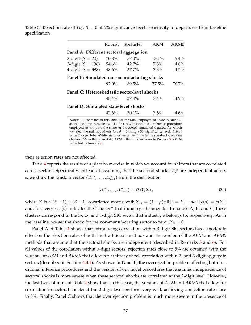
We illustrate the finite-sample properties of our novel inference procedure by implementing it onthe same placebo samples that we use to illustrate the bias of usual standard error formulas. Our newformulas deliver estimates that are close to the true standard deviation of the OLS estimator acrossthe placebo samples; consequently, when applied to perform significance tests, they yield rejectionrates that are close to the nominal significance level. As predicted by the theory, our standard errorformula remains accurate in the presence of a state-level term in the regression residuals, and nomatter whether the shifters Xs are homoskedastic or heteroskedastic. When the number of sectorsis small or a sector is significantly larger that the other ones, our method overrejects relative to thenominal significance level, but it still attenuates the overrejection problem in comparison to usualstandard error formulas.

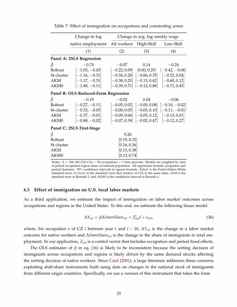
In the final part of the paper, we illustrate the implications of our new inference procedure forthree popular applications of shift-share regressions. First, we the study of the effect of changes insector-level Chinese import competition on labor market outcomes across U.S. Commuting Zones, asin Autor, Dorn and Hanson (2013). Second, we use changes in sector-level national employment toestimate the elasticity of regional employment to regional average wages, as in Bartik (1991). Lastly,we use changes in the stock of immigrants from various origin countries to investigate the impactof immigration on employment and wages across occupations and Commuting Zones in the UnitedStates, as in the literature pioneered by Altonji and Card (1991) and Card (2001).

In these applications, our proposed confidence intervals are substantially wider than those implied

3Software implementing our confidence intervals is available at https://github.com/kolesarm/BartikSE.4This result is similar to that in Barrios et al. (2012), who consider cross-section regressions estimated at an individual

level when the variable of interest varies only across groups of individuals. They show that, as long as the shifter of interestis as good as randomly assigned and independent across these individuals’ groups, standard errors clustered on groupsare valid under any correlation structure of the residuals.

5In an extension, we also provide confidence intervals that are valid when the shifters Xs are independent only across“clusters” of sectors, allowing thus for any correlation of these shifters across sectors belonging to the same “cluster”. Wealso extend our methodology to settings in which the shift-share regressor is not the treatment of interest but an instrumentin an instrumental variables estimator.

3

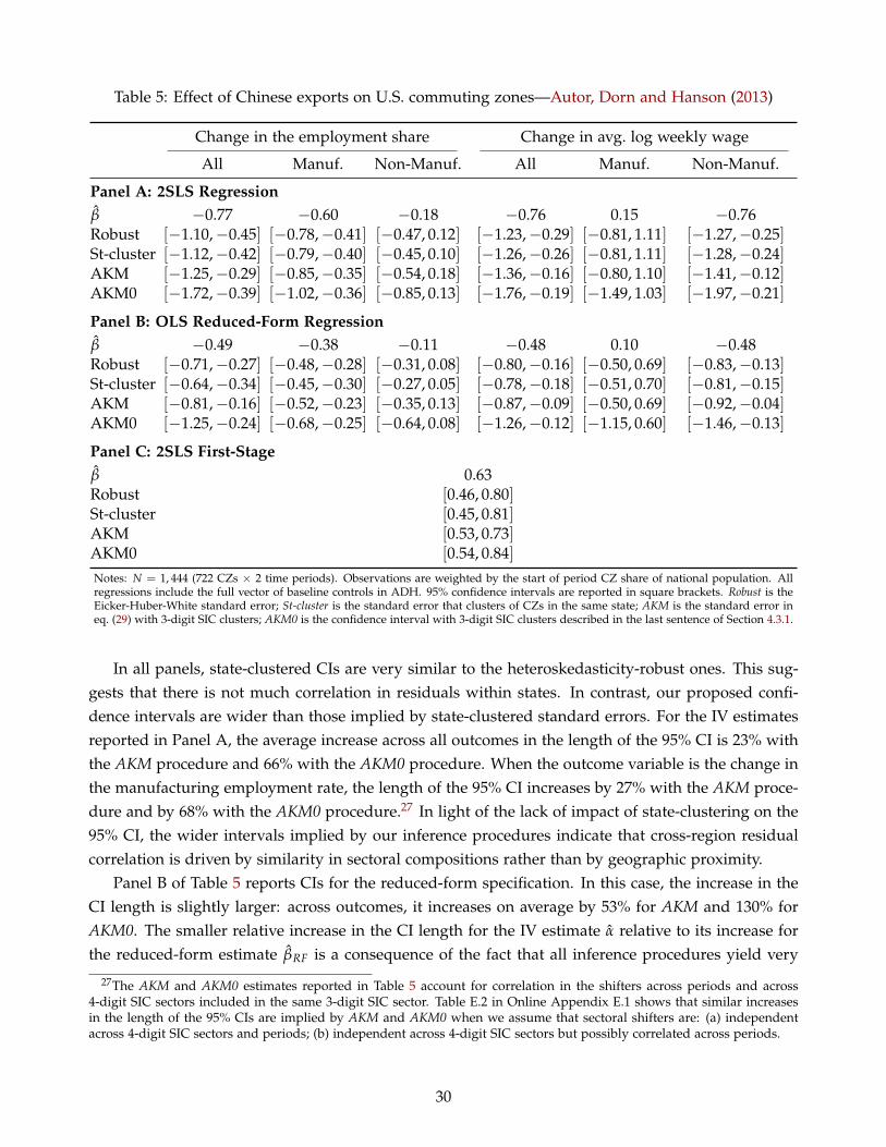
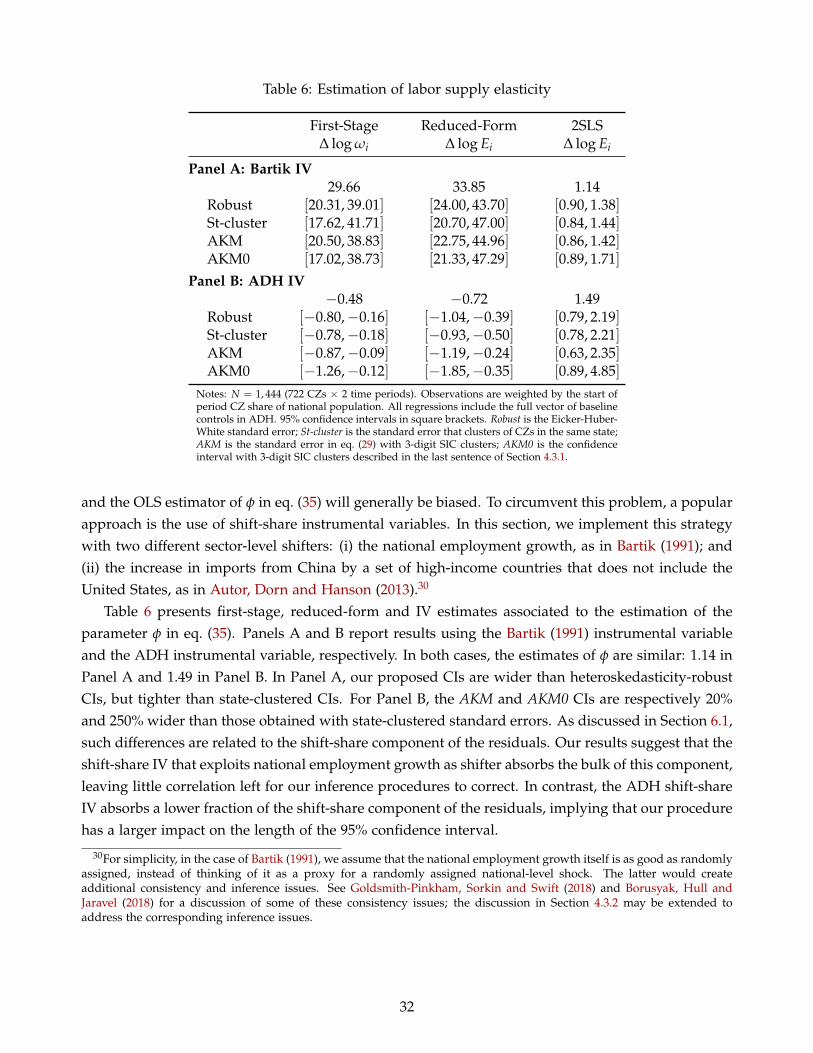
by state-clustered or heteroscedasticity-robust standard errors. In particular, the 95% confidenceintervals for the estimated effects of Chinese competition on local labor markets increase by 20%–70%,although these effects remain statistically significant. We obtain similar increases in the length of the95% confidence interval for the estimated impact of immigration shocks, which are 20%–120% widerthan those implied by traditional methods. In contrast, our confidence intervals for the labor supplyelasticity estimated using the procedure in Bartik (1991) are almost identical to those constructedusing standard approaches; intuitively, the sectoral shifter used in this application—the change innational employment by sector—soaks up most sectoral shocks affecting the outcome variable and,consequently, no shift-share structure is left in the regression residuals.6

Shift-share designs have been applied to estimate the effect of a wide range of shocks. Since theapplications are too numerous to comprehensively enumerate, let us list a few selective examples. Inseminal papers, Bartik (1991) and Blanchard and Katz (1992) use shift-share strategies to analyze theimpact on local labor markets of shifters measured as changes in national sectoral employment. Morerecently, shift-share strategies have been applied to investigate the local labor market consequencesof various observable shocks, including international trade competition (Topalova, 2007, 2010; Kovak,2013; Autor, Dorn and Hanson, 2013; Dix-Carneiro and Kovak, 2017; Pierce and Schott, 2017), creditsupply (Greenstone, Mas and Nguyen, 2015), technological change (Acemoglu and Restrepo, 2017,2018), and industry reallocation (Chodorow-Reich and Wieland, 2018). Shift-share regressors havealso been used to study the impact of the same shocks on other outcomes, such as political prefer-ences (Autor et al., 2017a; Che et al., 2017; Colantone and Stanig, 2018), marriage patterns (Autor,Dorn and Hanson, 2018), crime levels (Dix-Carneiro, Soares and Ulyssea, 2017), and innovation (Ace-moglu and Linn, 2004; Autor et al., 2017b). Shift-share regressors have been extensively used as wellto estimate the impact of immigration on labor markets, as in Card (2001) and many other papersfollowing his approach; see reviews of this literature in Lewis and Peri (2015) and Dustmann, Schön-berg and Stuhler (2016). Furthermore, recent papers have explored versions of shift-share strategiesto estimate the effect on firms of shocks to outsourcing costs and foreign demand (Hummels et al.,2014; Aghion et al., 2018). In addition to using shift-share designs to estimate the overall impact ofa shifter of interest, other work has used these designs as part of a more general structural estima-tion approach; see Diamond (2016), Adão (2016), Galle, Rodríguez-Clare and Yi (2017), Burstein et al.(2018b), Bartelme (2018). Baum-Snow and Ferreira (2015) review additional applications of shift-shareinstrumental variables in the context of urban economics.7 Independently of the aim of the researcherwhen estimating a shift-share regression, and of the interpretation of the estimand β in eq. (1), usualstandard errors formulas will generally be biased and, as long as the restrictions we impose on thedata generating process hold, our novel inference procedures will be asymptotically valid.

Our paper is related to three other papers studying the statistical properties of shift-share specifi-

6To illustrate this point, we estimate the same inverse labor supply elasticity using instead the shift-share instrument inAutor, Dorn and Hanson (2013). The sector shifter in this case—changes in trade flows from China to developed countriesother than the U.S.—leaves in the regression residual other sectoral shocks affecting U.S. labor markets; consequently, ourconfidence intervals are in this case 20%–250% wider than those implied by traditional inference procedures.

7Several papers use a shift-share approach that treats the shifters as unobserved, and for this reason uses the sharesdirectly as regressors. This approach has been applied to investigate the impact of technological shifters (Autor and Dorn,2013), credit supply shifters (Huber, 2018), and immigration shifters (Card and Dinardo, 2000; Monras, 2015). We treat thesectoral shares Xs as observed and leave the extension to the unobserved case to future work.

4

cations. First, Goldsmith-Pinkham, Sorkin and Swift (2018) focus on the case in which the shift-shareregressor is used as an instrumental variable. Within this setting, these authors study the usage of thefull vector of shares (wi1, . . . , wiS) as an instrument for the endogenous treatment, and they concludethat this approach requires that this vector of shares be as good as randomly assigned conditional onthe shifters, and independent across regions or clusters of regions. Given our interest in exploring theimpact of a specific set of shifters, rather than the impact of a set of shares, this approach is not attrac-tive in our setting. That said, there may be other settings in which this approach is more appealing.Second, Borusyak, Hull and Jaravel (2018), also focusing on the use of a shift-share regressor as aninstrumental variable, show that it is a valid instrument if the set of shifters is as good as randomlyassigned conditional on the shares, and discuss consistency of the instrumental variables estimator inthis context. Our approach to inference follows their identification insight; this way of thinking aboutthe shift-share design is also natural given our economic model. Third, Jaeger, Ruist and Stuhler(2018) study complications with the shift-share instrument when it is correlated over time and thereis a sluggish adjustment of the outcome variable to changes in it.

The rest of this paper is organized as follows. Section 2 presents the results of a placebo exerciseillustrating the properties of inference procedures previously used in the literature on shift-sharedesigns. Section 3 introduces our stylized economic model and maps its implications into a potentialoutcome framework. Section 4 establishes the asymptotic properties of the OLS estimator of β ineq. (1), and provides a consistent estimator of its standard error. Section 5 presents the results of aplacebo exercise in which we illustrate the performance of our novel inference procedures. Section 6revisits the conclusions from several prior applications of shift-share regression analysis, and Section 7concludes. Appendix A includes a microfoundation for the stylized economic model introduced inSection 3, and Appendix B contains proofs for all propositions in Section 4. Additional results arecollected in Online Appendices C, D and E.

2 Overrejection of usual standard errors: placebo evidence

In this section, we implement a placebo exercise to evaluate the finite-sample performance of thetwo inference methods most commonly applied in shift-share regression designs: (a) Eicker-Hubert-White—or heteroskedasticity-robust—standard errors, and (b) standard errors clustered on groupsof regions geographically close to each other. In our placebo, we regress observed changes in U.S.regional labor market outcomes on a shift-share regressor that is constructed by combining actual dataon initial sectoral employment shares for each region with randomly generated sector-level shocks.We describe the setup in Section 2.1 and summarize the results in Section 2.2.

2.1 Setup and Data

We generate 30, 000 placebo samples indexed by m. Each of them contains N = 722 regions andS = 397 sectors. We identify each region i with a U.S. Commuting Zone (CZ), and each sector s witheither a 4-digit SIC manufacturing industry or an aggregated non-manufacturing sector. We indexmanufacturing industries by s = 1, . . . , S− 1 and the non-manufacturing sector by s = S.

5

Using the notation introduced in eq. (1), each placebo sample m has identical values of the shares{wis}N,S

i=1,s=1, the outcomes {Yi}Ni=1, and the non-manufacturing shifter XS; the placebo samples differ

exclusively in the vector of shifters for the manufacturing sectors (Xm1 , . . . ,Xm

S−1). Specifically, theshares correspond to employment shares in 1990, the outcomes correspond to changes in employmentrates and average wages for different subsets of the population between 2000 and 2007, and theshifter for the non-manufacturing sector is always set to zero, XS = 0. The vector of shifters for themanufacturing sectors (Xm

1 , . . . ,XmS−1) is drawn i.i.d. from a normal distribution with zero mean and

variance var(Xms ) = 5 in each placebo sample m. Because the shifters are independent of both the

outcomes and the shares, the parameter β is zero in every placebo sample m (note it doesn’t matterwhat the dependence structure between the outcomes and shares themselves is).

For each placebo sample m, given the observed outcome Yi, the generated shift-share regressorXm

i and a vector of controls Zi including only an intercept, we compute the OLS estimate of β,the heteroskedasticity-robust standard error (which we label as Robust), and the standard error thatclusters CZs in the same state (with label St-cluster).

Our main source of data on employment shares is the County Business Patterns, and our measuresof changes in employment rates and average wages are based on data from the Census IntegratedPublic Use Micro Samples in 2000 and the American Community Survey for 2006 through 2008.Given these data sources, we construct our variables following the procedure described in the OnlineAppendix of Autor, Dorn and Hanson (2013).8

2.2 Results

Table 1 presents the median and standard deviation of the empirical distribution of the OLS estimatesof β across the 30,000 placebo samples, along with the median length of the different standard errorestimates, and rejection rates for 5% significance level tests of the null hypothesis H0 : β = 0.

The shifters have no effect on the outcomes and column (1) of Table 1 shows that, up to simulationerror, the average of the estimated coefficients is indeed zero for all outcomes. Column (2) reportsthe standard deviation of the estimated coefficients. This dispersion is the target of the estimatorsof the standard error of the OLS estimator.9 Columns (3) and (4) report the median standard errorfor Robust and St-cluster procedures, respectively, and show that both standard error estimators aredownward biased relative to the standard deviation of the OLS estimator. On average across alloutcomes, the median magnitude of the heteroskedasticity-robust and state-clustered standard errorsare, respectively, 41% and 30% lower than the true standard deviation.

The downward bias in the Robust and St-cluster standard errors translates into a severe overrejec-tion of the null hypothesis H0 : β = 0. Since the true value of β equals 0 by construction, a correctlybehaved test statistic should generate a rejection rate of 5%. Columns (5) and (6) in Table 1 showthat traditional standard error estimators yield much higher rejection rates. For example, when theoutcome variable is the CZ’s employment rate, the rejection rate for a 5% significance level for thenull hypothesis H0 : β = 0 is 49.1% and 38.3% when Robust and St-cluster standard errors are used,

8We are very grateful to the authors for sharing their code and datasets with us.9 Figure D.1 in Online Appendix D.2 reports the empirical distribution of the OLS estimates when the dependent variable

is the change in each CZ’s employment rate. Its distribution resembles a normal distribution centered around β = 0.

6

Table 1: Standard errors and rejection rate of the hypothesis H0 : β = 0 at 5% significance level.

Estimate Median std. error Rejection rate

Mean Std. dev Robust St-cluster Robust St-cluster(1) (2) (3) (4) (5) (6)

Panel A: Change in the share of working-age populationEmployed −0.01 2.00 0.74 0.92 49.1% 38.3%Employed in manufacturing −0.01 1.88 0.60 0.77 55.6% 44.4%Employed in non-manufacturing 0.01 0.94 0.58 0.67 23.0% 17.4%

Panel B: Change in average log weekly wageEmployed −0.02 2.68 1.02 1.34 47.2% 34.1%Employed in manufacturing −0.03 2.93 1.69 2.11 26.4% 16.8%Employed in non-manufacturing −0.02 2.65 1.05 1.33 45.4% 33.5%

Notes: For the outcome variable indicated in the first column, this table indicates the median and standard deviation of the OLSestimates across the placebo samples (columns (1) and (2)), the median standard error estimates (columns (3) and (4)), and thepercentage of datasets for which we reject the null hypothesis H0 : β = 0 using a 5% significance level test (columns (5) and (6)).Robust is the Eicker-Huber-White standard error, and St-cluster is the standard error that clusters CZs in the same state. Resultsare based on 30,000 simulation draws.

respectively. These rejection rates are very similar when the dependent variable is instead the changein the average log weekly wage.

These results are quantitatively important. To see this, consider the following thought-experiment.Suppose we were to provide our 30, 000 simulated samples to 30, 000 researchers without disclosingto them the origin of the data. Instead, we would tell them that the shifters correspond to changes ina sectoral shock of interest—for instance, trade flows, tariffs, national employment or the number offoreign workers employed in an industry. If these researchers set out to evaluate the impact of theseshocks on U.S. CZs using standard inference procedures with a 5% significance level test, then over athird of them would conclude that our computer generated shocks had a statistically significant effecton the evolution of employment rates between 2000 and 2007.

The following remark summarizes the results of our placebo exercise.10

Remark 1. In shift-share regressions, traditional inference methods suffer from a severe overrejection problemand yield confidence intervals that are too short.

To develop some intuition on the source of this overrejection problem, note that the standard errorestimators commonly applied in shift-share regression designs assume that the regression residualsare either independent across all regions (for Robust), or between geographically defined regionalgroups (for St-cluster). Given that shift-share regressors are correlated across regions with similar sec-toral employment shares {wis}S

s=1, these methods generally lead to a downward bias in the standarderror estimate whenever regions with similar sectoral employment shares {wis}S

s=1 also tend to havesimilar regression residuals. In the next section, we consider the implications of a stylized economicmodel, and show that such correlations between the regression residuals are likely to arise because

10In Section 5, we extend our analysis to a number of modifications of this baseline setup, including alternative definitionsof sectors and regions, allowing for a non-zero shock to the non-manufacturing sector, and allowing for correlations betweenthe shocks to different sectors. The overrejection problem is always at least as severe as in this baseline setup.

7

regions are generally exposed to unobserved sector-level shocks, in addition to the observed shocksXs. Consequently, whenever a researcher is running a shift-share regression, both heteroskedasticity-robust and state-clustered standard errors will generally be biased downwards.

3 Stylized economic model

This section presents a stylized economic model mapping sector-level shocks to labor market out-comes for a set of regional economies. The aim of the model is twofold. First, we show that theimpact of sectoral shifters on regional labor market outcomes have a shift-share structure, with het-erogeneous effects across regions and sectors. Second, we show that unobserved sectoral shiftersintroduce correlation in the regression residuals across regions with similar observed shares. We de-scribe the model fundamentals in Section 3.1, discuss its main implications for the impact of sectoralshocks in Section 3.2, and map these implications to a potential outcome framework in Section 3.3.

3.1 Environment

We consider an economy with multiple sectors s = 1, . . . , S and multiple regions i = 1, . . . , J. Weassume that the labor demand in sector s and region i, Lis, is given by

log Lis = −σs log ωi + log Dis, σs > 0, (3)

where ωi is the wage rate in region i, σs is the sector-specific labor demand elasticity, and Dis areregion- and sector-specific labor demand shifters. The shifter Dis may account for multiple sectoralcomponents. Since our analysis focuses on the impact of one particular sectoral component, wedecompose Dis into an observed shifter of interest, χs, other (potentially unobserved) shifters thatvary at a sectoral level and are grouped into µs, and a residual region- and sector-specific shifter ηis.That is, without loss of generality, we write

log Dis = ρs log χs + log µs + log ηis. (4)

We assume that the labor supply in region i is given by

log Li = φ log ωi + log vi, φ > 0, (5)

where φ is the labor supply elasticity, and vi is a region-specific labor supply shifter.Workers are assumed to be immobile across regions, but freely mobile across sectors. Thus, we

define the equilibrium as the wages {ωi}Ji=1 that satisfy the following market clearing condition:

Li =S

∑s=1

Lis, i = 1, . . . , J. (6)

There are multiple microfoundations that are consistent with the labor demand in eq. (3) and thelabor supply in eq. (5). For our purposes, the different labor demand microfoundations are important

8

only to the extent that they affect the interpretation of the sector- and region-specific labor demandshifter Dis. For example, one could assume that labor is the only factor of production and that everyregion i is a closed economy and, in this case, Dis may account both for demand shifters for sector-specific goods and for sector-specific productivity shifters. Similarly, as we show in Appendix A, wemay also allow goods to be freely traded across regions and assume that a subset of the J regions aresmall open economies; in this case, the shifter Dis for these small open economies will account forthe world price of sector s, which will itself capture the impact of foreign demand and productivityshocks. We also show in Appendix A that the labor supply in eq. (5) may be derived as the outcome ofthe utility maximization problem of individuals who, conditional on being employed, are indifferentabout the sector of employment, but have heterogeneous disutilities of being employed at all.

3.2 Labor market impact of sectoral shocks

We assume that, in any period, our model characterizes the labor market equilibrium in every regioni = 1, . . . , J and that, across periods, changes in the labor market outcomes {ωi, Li}J

i=1 are due tochanges in the sectoral shifter of interest, {χs}S

s=1, other potential sectoral shifters {µs}Ss=1, sector- and

region-specific shifters {ηis}J,Si=1,s=1, and labor supply shifters, {vi}J

i=1. Specifically, in every period,the values of these shifters correspond to draws from an unknown joint distribution F(·):

({χs, µs}Ss=1, {ηis}J,S

i=1,s=1, {vi}Ji=1) ∼ F(·). (7)

We use z = log(zt/z0) to denote log-changes in a variable z between some initial period t = 0 andany other period t. Up to a first-order approximation around the initial equilibrium, eqs. (3) to (6)imply that the change in employment in region i is

Li =S

∑s=1

l0is [βisχs + λiµs + λiηis] + (1− λi) vi, (8)

where l0is is the initial employment share of sector s in region i, λi ≡ φ

[φ + ∑s l0

isσs]−1, and βis ≡ ρsλi.

According to eq. (8), the impact of sectoral shifters on equilibrium employment in region i dependsboth on the initial sectoral employment shares {l0

is}Ss=1, and the region- and shifter-specific elasticities

{βis, λi}Ss=1. Consequently, the employment change in eq. (8) includes several components with a

shift-share structure: the “share” term is always the initial employment share in a sector l0is, and the

“shift” term is either the sectoral shock of interest, χs, or alternative labor demand shocks, µs. Thisstructure with multiple shift-share terms, some of them observed and others potentially unobserved,is central to understanding the results presented in Section 2.

Notice also that, even conditional on the initial employment share l0is, the impact of a sector s

shifter on region-i’s employment may be heterogeneous across sectors and regions: βis may varyacross i and s.11 While standard datasets will usually contain information on the initial employmentshares for every sector and region {l0

is}J,Si−1,s=1, each parameter βis is not generally known or directly

11In our model, βis does not vary across regions or sectors if and only if all sectors have the same labor demand elasticity,σs = σ, and shock pass-through, ρs = ρ.

9

observed, and thus, the impact of the sectoral shifters need to be estimated.We summarize this discussion in the following remark:

Remark 2. The change in regional employment will generally combine multiple shift-share terms, and theshifter effects depend on parameters that are heterogeneous across sectors and regions.

The property that the impact of a shifter in sector s on employment in region i may be written asl0isβis that underlies Remark 2 does not depend on the particular microfoundation of the labor demand

and labor supply expressions in eqs. (3) and (5). The only difference across these microfoundationsis how βis depends on the structural parameters of each microfounded model.

Besides the illustrative example of a possible microfoundation described in Appendix A, we pro-vide alternative microfoundations in Online Appendices C.2 and C.3. Specifically, we show in OnlineAppendix C.2 that eq. (8) is consistent with a Jones (1971) model featuring sector-specific inputs ofproduction. In Online Appendix C.3, we show that eq. (8) also arises in a Roy (1951) model in whichworkers have heterogeneous preferences for being employed in the different sectors.

We also extend our model in Online Appendix C.4 to allow for migration across regions. In thiscase, the change in regional employment Li in any given region i = 1, . . . , J depends not only on theregion’s own shift-share terms included in eq. (8), but also on an endogenous component, commonto all regions, that combines the shift-share terms corresponding to all regions i = 1, . . . , J. Thus, inthe presence of migration, l0

isβis is the partial effect of the shifter χs on local employment that ignorescross-regional spillovers; consequently, it will only capture the differential effect of the sector-specificshock χs on region i relative to all other regions. However, once we condition on fixed effects thatabsorb these cross-regional spillovers, Remark 2 remains valid for the model with migration.

3.3 From theory to inference

We build on the insights of Section 3.2 to propose a general framework to estimate the effect of shifterson an outcome of interest that varies at a different level than these shifters. For concreteness, we referto the level at which the shifters vary as sectors, and the level at which the outcome varies as regions,but our results do not depend on these particular labels.

To make precise what we mean by “the effect of shifters on an outcome”, we use the potentialoutcome notation, writing Yi(x1, . . . , xS) to denote the potential (counterfactual) outcome that wouldoccur in region i if the shocks to the S sectors were exogenously set to {xs}S

s=1. Consistently witheq. (8), we assume that the potential outcomes are linear in the shocks,

Yi(x1, . . . ,xS) = Yi(0) +S

∑i=1

wisxsβis, whereS

∑s=1

wis = 1, (9)

and Yi(0) ≡ Yi(0, . . . , 0) denotes the potential outcome in region i when all shocks {xs}Ss=1 are set to

zero. According to eq. (9), increasing xs by one unit while holding the shocks to the other sectorsconstant, leads to an increase in region i’s outcome of wisβis units. This is the treatment effect of xs

on Yi(x1, . . . ,xS). The actual (observed) outcome is given by Yi = Yi(X1, . . . ,XS), which depends on

10

the realization of the shifters X1, . . . ,XS. To map eq. (8) into eq. (9), define

Yi = Li, wis = l0is, xs = χs, Yi(0) =

S

∑s=1

l0isλi(µs + ηis) + (1− λi) vi. (10)

Observe that Yi(0) aggregates all shifters other than the sectoral shifter of interest χs.In the rest of the paper, we assume that we observe data for N regions and S sectors on the sectoral

shifters Xs, the regional outcomes Yi, and the region-sector shares wis.12,13 We are interested in theproperties of the OLS estimator β of the coefficient on the shift-share regressor Xi = ∑S

s=1 wisXs in aregression of Yi onto Xi. To help us focus on the key conceptual issues, we abstract away from anyadditional covariates or controls for now, and assume that Xs and Yi have been demeaned, so that wecan omit the intercept in a regression of Yi on Xi (see Section 4.2 for the case with controls). The OLSestimator of the coefficient on Xi in this simplified setting is given by

β =∑N

i=1 XiYi

∑Ni=1 X2

i

, (11)

and we can write the regression equation as

Yi = βXi + εi, where Xi ≡S

∑s=1

wisXs,S

∑s=1

wis = 1, (12)

where β denotes the population analog of β.The definition of the estimand β and the properties of the estimator β will depend on: (a) what

the population of interest is; and (b) how we think about repeated sampling. For (a), we definethe population of interest to be the observed set of N regions, as opposed to focusing on a largesuperpopulation of regions from which the N observed regions are drawn. Consequently, we areinterested in the parameters {βis}N,S

i=1,s=1 and the treatment effects {wisβis}N,Si=1,s=1 themselves, rather

than the distributions from which they are drawn, which would be the case if we were interested in asuperpopulation of regions.14 For (b), given our interest on estimating the ceteris paribus impact of aspecific set of shocks X1, . . . ,XS, we consider repeated sampling of these shocks, while holding fixedthe shares wis, the parameters βis, and the potential outcomes Yi(0).

Given our assumptions on the population of interest and on the type of repeated sampling, theestimand β is defined as the population analog of eq. (11) under repeated sampling of the shocks Xs:

β =∑N

i=1 E[XiYi | F0]

∑Ni=1 E[X2

i | F0], with F0 = {Yi(0), βis, wis}N,S

i=1,s=1, (13)

12We can think of the N observed regions as a subset of the J regions existing worldwide and whose labor marketequilibrium is described in Sections 3.1 and 3.2.

13For simplicity, we assume that we have data on the shifters Xs directly, rather than possibly noisy estimates of them.14This definition of the population of interest is common in applications of the shift-share approach. For example, the

abstract of Autor, Dorn and Hanson (2013) reads: “We analyze the effect of rising Chinese import competition between1990 and 2007 on U.S. local labor markets”. Similarly, the abstract of Dix-Carneiro and Kovak (2017) reads: “We study theevolution of trade liberalization’s effects on Brazilian local labor markets” (emphases added).

11

and, given eqs. (9) and (12), the regression error εi is then defined as the residual

εi = Yi − Xiβ = Yi(0) +S

∑i=1

wisXs(βis − β), (14)

where β is defined as in eq. (13).Thus, the statistical properties of the regression residual εi depend on the properties of the po-

tential outcome Yi(0), the shifters {Xs}Ss=1, the shares {wis}N,S

i=1,s=1, and the difference between theparameters {βis}N,S

i=1,s=1 and the estimand β. Importantly, the potential outcome Yi(0) will generallyincorporate terms that have a shift-share structure analogous to that of the regressor of interest, Xi.Specifically, as illustrated in eq. (10), the model introduced in Section 3.1 implies that Yi(0) includesa weighted average of unobserved sectoral labor-demand shocks, ∑S

s=1 l0isλiµs. Hence, if two regions

i and i′ have similar shares {l0is}S

s=1 and {l0i′s}S

s=1, they will tend to have similar regressors Xi and Xi′

and similar potential outcomes Yi(0) and Yi′(0). It then follows from eq. (14) that the residuals εi andεi′ will be correlated.15

We summarize this discussion in the following remark.

Remark 3. Correctly performing inference for the coefficient on a shift-share regressor β requires taking intoaccount that the regression residuals will generally inherit the same shift-share structure.

Remark 3 has important implications for estimating the variability of β across samples. In partic-ular, traditional inference procedures do not account for correlation in εi among regions with similarshares and, therefore, tend to underestimate the variability of β. As we discuss in all remainingsections of the paper, this is the main reason for the overrejection problem described in Section 2.

4 Asymptotic properties of shift-share regressions

In this section, we formulate the statistical assumptions that we impose on the data generating pro-cess (DGP), present asymptotic results that we derive using these assumptions, and use the modelintroduced in Section 3.1 to provide an economic interpretation for these assumptions. We first con-sider in Section 4.1 the simple case in which there is a single regressor with a shift-share structureand no controls, as in Section 3.3. We introduce controls in Section 4.2. Section 4.3 considers furtherextensions. All proofs and technical details are in Appendix B.

Following the notation introduced in Section 3.3, we write sector-level variables (such as theshocks Xs) in script font style and region-level aggregates (such as Xi) in normal style. To compactlystate our assumptions and results, we use standard matrix and vector notation. In particular, for a(column) L-vector Ai that varies at the regional level, A denotes the N × L matrix with the ith rowgiven by A′i. For an L-vector As that varies at the sectoral level, A denotes the S× L matrix with thesth row given by A ′s. If L = 1, then A and A are an N-vector and an S-vector, respectively. Let Wdenote the N× S matrix of shares, so that its (i, s) element is given by wis, and let B denote the N× Smatrix with (i, s) element given by βis.

15As we discuss in Section 4.2, when controls are included, this conclusion will still hold unless the controls account forall sectoral shocks other than {Xs}S

s=1 that affect the outcome.

12

4.1 No controls

We study here the statistical properties of the OLS estimator in eq. (11). We assume that, conditionallyon the matrix of shares W, the shocks are as good as randomly assigned in that they are independentof the potential outcomes Yi(x1, . . . ,xS). Formally, given the definition of the potential outcomes ineq. (9), we assume

(Y(0), B) ⊥⊥X |W. (15)

In the next subsection, we weaken this assumption by assuming that the shocks are as good asrandomly assigned conditionally on some controls.

As discussed in Section 3.3, we consider the statistical properties of β under repeated samplingof the shocks X, and condition on the realized values of the shares and on the potential outcomes.This approach is analogous to the randomization-style inference in the literature on inference inrandomized controlled trials (see Imbens and Rubin, 2015, for a review); it leverages the randomassignment assumption in eq. (15), and ensures that the standard errors that we derive will remainvalid under any dependence structure between the shares wis across sectors and regions, and underany correlation structure of the potential outcomes Yi(0), or equivalently, of the regression errorsεi, across regions. In particular, this approach allows (but does not require) the residual to have ashift-share structure.

We consider asymptotics with the number of sectors going to infinity, S → ∞, and assume thatN → ∞ as S → ∞. Formally, the number of regions N thus depends on S, but we keep thisconditioning implicit. We do not restrict the ratio N/S, so that the number of regions may growat a faster rate than the number of sectors. The assumptions needed for the propositions beloware collected in Appendix B.1. The key assumption underlying our approach to inference is thatthe shocks (X1, . . . ,XS) are independent across s conditional on the shares W (see Assumption 1(ii)in Appendix B.1). In contrast, Yi(0) and the shares wis can be correlated in an arbitrary manneracross i. We also do not require X, or any other variables, to be identically distributed—the sectorsand regions may be heterogeneous.

The main regularity condition that we need is that each sector is asymptotically negligible in thesense that maxs ns/N → 0, where ns = ∑N

i=1 wis is the aggregate “size” of sector s in the populationof interest (see Assumption 2(ii) in Appendix B.1). It generalizes the standard consistency conditionin the clustering literature that the largest cluster be asymptotically negligible. To see the connection,consider the special case with “concentrated sectors”, in which each region i specializes in one sectors(i). Then wis = 1 if s = s(i) and wis = 0 otherwise, and ns is the number of regions that specializein sector s. In this case, Xi = Xs(i), so that, if eq. (15) holds, β is equivalent to an OLS estimatorin a randomized controlled trial in which the treatment varies at a cluster level; here the sth clusterconsists of regions that specialize in sector s. The condition maxs ns/N → 0 then reduces to theassumption that the largest cluster be asymptotically negligible.

Proposition 1. Suppose Assumptions 1 and 2 in Appendix B.1 hold. Then

β =∑N

i=1 ∑Ss=1 πisβis

∑Ni=1 ∑S

s=1 πis, and β = β + op(1), (16)

13

where πis = w2is var(Xs |W).

This proposition gives two results. First, it shows that the estimand β in eq. (13) can be expressedas a weighted average of the region- and sector-specific parameters {βis}N,S

i=1,s=1, with weights thatare increasing in the shares and variance of the shock. Second, it shows that the OLS estimator β

converges to this estimand as S → ∞. The special case with concentrated sectors is again useful tounderstand Proposition 1. Fully concentrated sectors imply that ∑S

s=1 πisβis = var(Xs(i) | W)βis(i)

and, therefore, the first result in Proposition 1 reduces to the standard result from the randomizedcontrolled trials literature with cluster-level randomization (with each “cluster” defined as all regionsspecialized in the same sector) that the weights are proportional to the variance of the shock.

The estimand β does not in general equal a weighted average of the heterogeneous treatmenteffects. As discussed earlier, the effect on the outcome in region i of increasing the value of the sectors shock in one unit is equal to wisβis; the total effect of increasing the shifters simultaneously inevery sector by one unit is ∑S

s=1 wisβis. Consequently, for a set of region- and sector-specific weights{ξis}N,S

i=1,s=1, the corresponding weighted average treatment effect is

τξ ≡∑N

i=1 ∑Ss=1 ξiswisβis

∑Ni=1 ∑S

s=1 ξis,

and a weighted total average treatment effect is τTζ = ∑N

i=1 ζi ∑Ss=1 wisβis, where {ζi}N

i=1 are regionalweights that sum to one. If βis is constant across i and s, βis = β, then β = τT

ζ , and τξ can beconsistently estimated as τξ = β ∑N

i=1 ∑Ss=1 ξiswis/ ∑N

i=1 ∑Ss=1 ξis. On the other hand, if βis varies across

regions and sectors, then it is not clear in general how to exploit knowledge of the estimand β definedin eq. (16) to learn something about τξ or τT

ζ . A special case in which it is possible to consistentlyestimate τξ arises when Xs is homoscedastic and ξis = wis; in this case, a consistent estimate is givenby τξ = β ∑N

i=1 ∑Ss=1 w2

isσ2/ ∑N

i=1 ∑Ss=1 wisσ

2, where σ2 is a consistent estimate of var(Xs).16

Under slight strengthening of the regularity conditions (see Assumption 3 in Appendix B.1), weobtain the following distributional result:

Proposition 2. Suppose Assumptions 1, 2 and 3 hold, and suppose that

VN =1

∑Ss=1 n2

svar

(N

∑i=1

Xiεi | Y(0), B, W

)

converges in probability to a non-random limit, where ns = ∑Ni=1 wis. Then

N√∑S

s=1 n2s

(β− β) = N

0,VN(

1N ∑N

i=1 X2i

)2

+ op(1).

16 In general, one could consistently estimate τξ or τTζ by imposing a mapping between βis and structural parameters

and obtaining consistent estimates of these structural parameters. However, since this mapping will vary across models,the consistency of such estimator will not be robust to alternative modeling assumptions, even if all these modeling as-sumptions predict an equilibrium relationship like that in eq. (8); e.g. see expressions for βis in Appendix A and in OnlineAppendices C.2 and C.3.

14

This proposition shows that β is asymptotically normal, with a rate of convergence equal toN(∑S

s=1 n2s )−1/2. If the sector sizes ns are all equal to N/S, the rate of convergence is equal to

√S.

However, if the sizes are unequal, the rate may be slower.According to Proposition 2, the asymptotic variance formula has the usual “sandwich” form. Since

Xi is observed, to construct a consistent standard error estimate, it suffices to construct a consistentestimate of VN , the middle part of the sandwich. Suppose that βis is common across regions andsectors, βis = β, then it follows from eq. (15) and the assumption that (X1, . . . ,Xs) are independentacross s that17

VN =∑S

s=1 var(Xs |W)R2s

∑Ss=1 n2

s, Rs =

N

∑i=1

wisεi. (17)

Replacing var(Xs |W) by X2s , and εi by the regression residual εi = Yi − Xi β, we obtain the standard

error estimate

se(β) =

√∑S

s=1 X2s R2

s

∑Ni=1 X2

i

, Rs =N

∑i=1

wisεi. (18)

To gain intuition for the expression in eq. (18), consider the case with concentrated sectors such thatthe formula becomes ∑S

s=1 X2s R2

s = ∑Ss=1(∑

Ni=1 I{s(i) = s}Xi εi)

2. In this special case, the standarderror formula in eq. (18) reduces to the usual cluster-robust standard error, allowing for arbitrarycorrelation across regions specialized in the same sector.18

When regions are not fully specialized in a sector, the standard error in eq. (18) accounts forthe fact that regions with similar sectoral composition will generally have similar errors; only in thespecial case in which the regression error εi = Yi(0) has no sectoral component (so there are nounobserved sector-level shocks), it will be the case that cov(Xiεi, Xjεj) = 0 for i 6= j. In contrast, theusual heteroscedasticity-robust standard error fails to account for this correlation. Standard errorsclustered by groups of regions defined by their geographical proximity will also generally fail toaccount for this correlation. In fact, they will only capture it if and only if all regions are fullyspecialized in a single sector and the sector of specialization is the same for regions belonging to thesame geographically defined cluster.

Remark 4. In the expression for VN in eq. (17), the only expectation is taken over Xs—we do not take anyexpectation over the shares wis or the residuals εi. This is because our inference is conditional on the realizedvalues of the shares and on the potential outcomes. In terms of the regression in eq. (12), this means thatwe consider properties of β under repeated sampling of Xi = ∑s wisXs conditional on the shares wis and onthe residuals εi (as opposed to, say, considering properties of β under repeated sampling of the residuals εi

conditional on Xi). As a result, our standard errors allow for arbitrary dependence between the residuals εi.17The standard error formula that we provide remains valid if βis is heterogeneous across regions and sectors, as long as

some mild restrictions on the form of heterogeneity apply; see Appendix B.6 for a discussion.18Thus, in the case with concentrated industries, the usual approach to inference that considers repeated sampling of εi,

holding the regressors constant, would deliver the same standard error formula if one assumed that εi were independentacross locations specializing in different industries.

15

4.1.1 Discussion of assumptions

In general, in order to identify a relationship as causal, one needs a random assignment assump-tion. In order to do inference and apply a central limit theorem, one needs an independence-typeassumption.19 In our case, the key identifying assumption is that the shifters {Xs}S

s=1 are as good asrandomly assigned conditional on the shares {wis}S,N

s=1,i=1 (see eq. (15)). This identification assump-tion has been previously suggested by Borusyak, Hull and Jaravel (2018). For inference, we alsorequire that the shocks are independent across sectors. As illustrated through the economic modelsdescribed in Appendix A and Online Appendix C, these assumptions generally imply restrictions onthe stochastic process of economic fundamentals. How strong these restrictions are will depend onthe specific context. For example, in a world in which all N regions of interest are closed economies,the only sectoral shocks are either productivity or preference shocks, and the shifters of interest arethe former, these assumptions require that, conditional on the shares, the productivity shocks are:(a) independent of preference shocks; and (b) independent across sectors. In Section 4.2, we illus-trate how to relax assumption (a) by incorporating controls into the regression specification and, inSection 4.3.2, we show how to relax it by using instrumental variables. Additionally, we show inSection 4.3.1 how to relax assumption (b) by allowing for a non-zero correlation in the sectoral shocksof interest within clusters of sectors.

Goldsmith-Pinkham, Sorkin and Swift (2018) investigate a different approach to identificationbased on the assumption that the shares (wi1, . . . , wiS) are as good as randomly assigned conditionalon the shifters Xs. For inference, this approach requires that the shares (wi1, . . . , wiS) be independentacross regions or clusters of regions. However, as illustrated through the stylized economic modelpresented in Section 3, these shares are generally equilibrium objects and, consequently, they areunlikely to be as good as randomly assigned. For instance, in the case of the environment describedin Section 3.1, under the assumption that σs = σ for all sectors, it holds that l0

is = D0is/(∑

Sk=1 D0

ik),where D0

is is the labor demand shifter of sector s in region i in the initial equilibrium. However, asshown in eqs. (4), (10) and (14), the regression residual εi accounts for changes in certain variablesthat also affect the demand shifter D0

is and, consequently, l0is will generally be correlated with εi unless

changes in those variables are independent of their past initial levels.20 Furthermore, as the demandshifters D0

is are likely to depend on terms that vary by sector (see eq. (4)), the labor shares l0is will

generally be correlated across all regions i = 1, . . . , N for a given sector s, complicating the task ofderiving valid inference procedures in this setting.

The results in Propositions 1 and 2 also require the assumption that maxs ns/N → 0. In terms ofthe economic model introduced in Section 3, this assumption imposes that no one sector dominatesthe others in terms of initial employment at the national level; i.e. ∑N

i=1 l0is is not too large for any one

sector. As we illustrate in Section 5.2, this condition is satisfied for the U.S. when only manufacturingsectors are taken into account; it would not hold if the non-manufacturing sector is included as one of

19For example, for inference on average treatment effects, which is commonly the goal when running a regression, oneassumes that the treatment is as good as randomly assigned conditional on controls, and typically also that the data onindividuals is i.i.d., which implies that the treatment is independent across individuals conditional on the controls.

20Importantly, the correlation between the shares {wis}Ss=1 and the regression residuals εi does not affect the consistency

of the OLS estimator of β if the shifters Xs are as good as randomly assigned conditional on the shares wis.

16

the S sectors incorporated into the analysis (unless the distribution of Xs for the non-manufacturingsector is degenerate at zero).21

Finally, Propositions 1 and 2 also require the number of sectors and the number of regions to go toinfinity. Shift-share designs are however sometimes used in settings in which the number of regionsor the number of sectors is small. Through placebo exercises, we illustrate in Section 5 the finite-sample properties of the standard error estimator introduced in eq. (18): our estimates are very closeto the true standard deviation of the estimator β for sample sizes employed in typical applications.

4.2 General case with controls

In many applications of shift-share regression designs, a K-vector of regional controls Zi is includedin the regression specification. We now study the properties of the OLS estimator of the coefficienton Xi in a regression of Yi onto Xi and Zi. To this end, let Z denote the N × K matrix with i-th rowgiven by Z′i , and let X = X − Z(Z′Z)−1Z′X denote an N-vector whose i-th element is equal to theregressor Xi with the controls Zi partialled out (i.e. the i-th residual from regressing X onto Z). Then,by the Frisch–Waugh–Lovell theorem, β is equivalent to

β =∑N

i=1 XiYi

∑Ni=1 X2

i

=X′YX′X

, (19)

and the OLS estimator of the coefficient on Zi is equivalent to

δ = (Z′Z)−1Z′(Y− Xβ).

The controls Z may play two roles. First, controls may be included to increase the precision of β.Second, and more importantly, they may be included to proxy for latent sector-level shocks {Zs}S

s=1

that have an independent effect on the outcome Y and are correlated with the shifters {Xs}Ss=1. In

the presence of such shocks, the shifters are only as good as randomly assigned conditional on them,and it is necessary to control for them in order to prevent omitted variable bias.

To account for the two possible roles that controls may play, we assume that the controls Zi admitthe decomposition

Zi =S

∑s=1

wisZs + Ui. (20)

If the kth component Zik of Zi is included for precision, then Zsk = 0 for all s = 1, . . . , S, and Zik isincluded because Yi(0) and Uik are correlated. This is the case, for instance, if Yi(0) and Uik containregional shocks that are independent of the sectoral shifters of interest X. If, on the other hand, Zik

is included to proxy for a latent shock Zs, then Uik represents the measurement error in Z whencontrolling for Z and Zik is a perfect only if Uik = 0.

21When analyzing the impact of international trade on regional labor market outcomes, it is standard to either setthe shock of the non-manufacturing sector to zero (Topalova, 2007, 2010; Autor, Dorn and Hanson, 2013; Hakobyan andMcLaren, 2016) or to remove the non-manufacturing sector from the analysis and rescale the shares of all manufacturingsectors so that they add up to one (Kovak, 2013). Either of these approaches will satisfy the restriction that maxs ns/N → 0.

17

With this setup, we replace eq. (15) with the assumption that

(U, Y(0), B) ⊥⊥X | Z, W, (21)

where Z denotes the S× K matrix with sth row given by Z′s, and U denotes the N-vector with i-thelement given by Ui.

To facilitate the interpretation of the condition in eq. (21), it is useful to consider a projectionof the regional potential outcomes onto the sectoral space. For simplicity, consider the case withconstant effects, βis = β, and suppose Ui = 0. Project Yi(0) onto the sector-level controls Zs, so thatwe can write Yi(0) = ∑S

s=1 wisZ′sκ + ηi. Then eq. (21) holds if the residuals ηi in this projection are

independent of X—if there are any other unobserved sector-level shocks that affect the outcomes(and are therefore in ηi), these must be unrelated to (Xs,Zs).

To ensure that it suffices to include the controls in the regression linearly (instead of having tocontrol for them non-parametrically), we additionally assume that the expectation of Xs conditionalon Zs is linear in Zs,

E[Xs | Z, W] = Z′sγ, (22)

where γ is a K-vector that equals 0 if and only if the scalar Xs is mean independent of the K-vectorZs. We then obtain the following generalization of Proposition 1:

Proposition 3. Suppose Assumptions 2 and 4 in Appendix B.1 hold, and that U′i γ = 0 for i = 1, . . . , N.Then,

β =∑N

i=1 ∑Ss=1 πisβis

∑Ni=1 ∑S

s=1 πis, and β = β + op(1), (23)

where πis = w2is var(Xs |W,Z).

The only difference with to Proposition 1 is that the weights πis now reflect the variance of Xs

conditional on Z and W, rather than just conditional on W. An additional assumption is the require-ment that U′i γ = 0 for all i. Effectively, this requires that, for each control k, either Uik = 0 for all i,so that Zik is a perfect proxy for the sector-level variables Z1k, . . . ,ZSk, or else γk = 0, so that Zsk isunrelated to Xs—the proxy need not be perfect in this case, since it is not necessary to control for Zsk

in the first place (including Zik in the regression only affects the precision, but not the consistency,of β). If U′i γ 6= 0, then there will be omitted variable bias due to inadequately controlling for theconfounders Z. This is analogous to the classic linear regression result that measurement error in acontrol variable leads to a bias in the estimate of the coefficient on the variable of interest.

To state the asymptotic normality result, we need to define the residual εi in the regression equa-tion Yi = Xiβ + Z′i δ + εi. To this end, let

δ = E[Z′Z]−1E[Z′(Y− Xβ)]

denote the population regression coefficient on Zi. We then define the regression residual as εi =

Yi − Xiβ− Z′i δ and obtain the following generalization of Proposition 2:

18

Proposition 4. Suppose Assumptions 2, 3, 4 and 5 in Appendix B.1 hold, and that U′i γ = 0 for i = 1, . . . , N.Suppose also that

VN =1

∑Ss=1 n2

svar

(∑

i(Xi − Z′i γ)εi | Y(0), B, U,Z, W

)

converges in probability to a non-random limit, and let ns = ∑Ni=1 wis. Then

N√∑S

s=1 n2s

(β− β) = N

(0,

VN( 1N ∑i X2

i

)2

)+ op(1).

Relative to Proposition 2, the only difference is that Xi in the definition of VN is replaced byXi − Z′i γ, and that Xi is replaced by Xi in the outer part of the “sandwich.”

To construct a consistent standard error estimate, similarly to the case without controls, it sufficesto construct a consistent estimate of VN , the middle part of the sandwich. We derive the standarderror formula under the assumption that βis = β for all i, s.22 Under this assumption, it follows fromeq. (21) and the assumption that (X1, . . . ,Xs) are independent across s that

VN =∑S

s=1 var(Xs |W,Z)R2s

∑Ss=1 n2

s, Rs =

N

∑i=1

wisεi, Xs = Xs −Z′sγ.

A plug-in estimate of Rs can be constructed by replacing εi with the estimated regression residualsεi = Yi − Xi β − Zi δ. To construct an estimate of the variance var(Xs | W,Z), we first project theconsistent estimate Xi of Xi − Z′i γ onto the sectoral space by regressing it onto the shares Wi,

X = (W ′W)−1W ′X, (24)

and we then estimate the variance var(Xs |W,Z) by X2. This leads to the standard error estimate

se(β) =

√∑S

s=1 X2s R2

s

∑Ni=1 X2

i

, Rs =N

∑i=1

wisεi. (25)

The next remark summarizes these steps:

Remark 5. To construct the standard error estimate in eq. (25):

1. Obtain the estimates β and δ by regressing Yi onto Xi = ∑s wisXs and the controls Zi. The estimate εi

corresponds to the estimated regression residuals.

2. Construct Xi, the residuals from regressing Xi onto Zi. Compute Xs, the regression coefficients fromregressing X onto W. This requires the share matrix W to be full rank, which itself requires N > S.

Plug the estimates εi, Xi, and Xs into the standard error formula in eq. (25).

22We discuss in Appendix B.6 the restrictions under which our standard error formula remains valid when the effects areheterogeneous.

19

Consider again the case with concentrated sectors. Suppose that Ui = 0 for all i, so that theregression of Yi onto Xi and Zi is identical to the regression of Yi onto Xs(i) and Zs(i). Then, thestandard error formula in eq. (25) reduces to the usual cluster-robust standard error, with clusteringon the sectors s(i).

It has been shown that the cluster-robust standard error is generally biased due to estimation noisein estimating εi, which can lead to undercoverage, especially in cases with few clusters (see Cameronand Miller, 2014 for a survey). Since the standard error in eq. (25) can be viewed as generalizing thecluster-robust formula, similar concerns arise in our setting. We therefore also consider a modificationseβ0(β) of se(β) that imposes the null hypothesis when estimating the regression residuals to reducethe estimation noise in estimating εi. In particular, to calculate the standard error seβ0(β) for testingthe hypothesis H0 : β = β0 against a two-sided alternative at significance level α, one replaces εi withεβ0,i, the residual from regressing Yi − Xiβ0 onto Zi (that is, εβ0,i is an estimate of the residuals withthe null imposed). The null is rejected if the absolute value of the t-statistic (β− β0)/seβ0(β) exceedsz1−α/2, the 1− α/2 quantile of a standard normal distribution (1.96 for α = 0.05). To construct aconfidence interval (CI) with coverage 1− α, one collects all hypotheses β0 that were not rejected. Itfollows from simple algebra that the endpoints of this CI are a solution to a quadratic equation, sothat they are available in closed form—one does not have to numerically search for all the hypothesesthat were not rejected. The next remark summarizes this procedure.

Remark 6 (Confidence interval with null imposed). To test the hypothesis H0 : β = β0 with significancelevel α, or equivalently, to check whether β0 lies in the confidence interval with confidence level 1− α:

1. Obtain the estimate β by regressing Yi onto Xi = ∑s wisXs and the controls Zi. Obtain the restrictedregression residuals εβ0,i as the residuals from regressing Yi − Xiβ0 onto Zi.

2. Construct Xi, the residuals from regressing Xi onto Zi. Compute Xs, the regression coefficients fromregressing X onto W (this step is identical to step 2 in Remark 5).

Compute the standard error as

seβ0(β) =

√∑S

s=1 X2s R2

β0,s

∑Ni=1 X2

i

, Rβ0,s =N

∑i=1

wisεβ0,i. (26)

Reject the null if |(β− β0)/seβ0(β)| > z1−α/2. A confidence set with coverage 1− α is given by all nulls thatare not rejected, CI1−α = {β0 : |(β− β0)/seβ0(β)| < z1−α/2}. This set is an interval with endpoints given by

β− A±

√A2 +

se(β)2

Q/(X′X)2, A =

∑Ss=1 X

2s Rs ∑i wisXi

Q, (27)

where Q = (X′X)2/z21−α/2 −∑S

s=1 X2s (∑i wisXi)

2 and se(β) and Rs are given in eq. (25).

Since in both εi and εβ0,i are consistent estimates of the residuals, both seβ0(β) and se(β) areconsistent estimates of the standard error and, consequently, yield tests and confidence intervals thatare asymptotically valid. The next proposition formalizes this result.

20

Proposition 5. Suppose that the assumptions of Proposition 4 hold, and that βis = β. Suppose also that N ≥S, W is full rank, and that either maxs ∑i|((W ′W)−1W ′)si| is bounded, or else that Ui = 0 for i = 1, . . . , N.Define X as in eq. (24), and let Rs = ∑N

i=1 wisεi, where εi = Yi − Xi β − Z′i δ, and β and δ are consistentestimators of δ and β. Then

∑Ss=1 X

2s R2

s

∑Ss=1 n2

s= VN + op(1). (28)

The additional assumption of Proposition 5 is that either maxs ∑i|((W ′W)−1W ′)si| is boundedor, else, Ui = 0 for all i. This assumption ensures that the estimation error in Xs that arises fromhaving to back out the sector-level shocks Zs from the controls Zi is not too large. If the sectors areconcentrated, then ((W ′W)−1W ′)si = I{s(i) = s}/ns, so that maxs ∑i|((W ′W)−1W ′)si| = 1, and theassumption always holds.

Although both standard errors seβ0(β) and se(β) are consistent (and one could further show thatthe resulting confidence intervals are asymptotically equivalent), they will in general differ in finitesamples. In particular, it can be seen from the formula in Remark 6 that the confidence interval withthe null imposed is not symmetric around β, but its center is shifted by A.23 As we show in Section 5,this recentering tends to improve the finite-sample coverage properties of the confidence interval. Onthe other hand, the confidence interval tends to be longer on average than that in Remark 5.

4.2.1 Discussion of assumptions

The role that controls play in our framework is twofold. First, the k-th element of the vector Zi mayproxy for the impact on region i of an unobserved sectoral shock (Z1k, . . . ,ZSk). In the context of themodel in Section 3, regional labor market outcomes are not only affected by the sectoral shifters ofinterest (χ1, . . . , χS), but also by other sectoral shocks accounted for by the composites (µ1, . . . , µS),as illustrated in eq. (4). When the regression of Yi on Xi does not include a vector of controls Zi,consistent estimation of β requires assuming that the vector of sectoral shocks of interest (χ1, . . . , χS)

is independent of all other sectoral shocks (µ1, . . . , µS). On the other hand, if we control for theimpact of the sectoral shocks (µ1, . . . , µS) on regional labor market outcomes through a regionalcontrol Zi = ∑S

s=1 wisµs, then the OLS estimator β will be consistent even if (µ1, . . . , µS) are notindependent of the sectoral shocks of interest (χ1, . . . , χS).

Second, each element of the vector Zi may proxy for regional shocks that, although independentof the sectoral shocks of interest Xs, have an effect on the outcome variable and, thus, enter theregression residual εi in eq. (12). Controlling for these shocks is not necessary for the consistencyof β, but including them increases its precision. An example of such a shock in the context of themodel in Section 3 is the region-specific labor supply shifter vi, as long as {vi}N

i=1 are independent ofthe shocks of interest {Xs}S

s=1. If this independence condition does not hold, then it is important tocontrol for these labor supply shocks in order to ensure consistency of β.

Even if all other sectoral shocks are independent of the shifters of interest, including controls thatproxy for them in the regression will reduce the correlation between residuals of regions with simi-

23This is analogous to the differences in likelihood models between confidence intervals based on the Lagrange multipliertest (which imposes the null and is not symmetric around the maximum likelihood estimate) and the Wald test (which doesnot impose the null and yields the usual confidence interval).

21

lar shares, and it may therefore attenuate the overrejection problem of traditional inference methodsdocumented in Section 2. In the limit, if the controls soak up all sectoral shocks, so that the residualsεi are independent across i, the usual heteroscedasticity-robust confidence intervals will give correctcoverage, and our confidence intervals will be asymptotically equivalent to them. However, since ourinference methods are valid whether or not there is shift-share structure in the residuals, we recom-mend that researchers always use them, in line with the practice of always clustering the standarderrors if the regressor of interest only varies at a group level.

4.3 Extensions

We now discuss two extensions of the basic setup: first, we weaken the assumption that (X1, . . . ,Xs)

are independent across s. Second, we consider using the shift-share regressor Xi as an instrument.

4.3.1 Clusters of sectors

Suppose that the sectors can be grouped into larger units, which we refer to as “clusters”, withc(s) ∈ {1, . . . , C} denoting the cluster that sector s belongs to; e.g., s may be a four-digit industry code,while c(s) is a three-digit code. With this structure, we replace here the assumption that the shocks Xs

are independent across sectors (Assumption 1(ii) in Appendix B.1 for the case without controls, andAssumption 4(ii) for the general case) with the assumption that, conditional on Z and W, the shocksXs and Xk are independent if c(s) 6= c(k) (for the case without controls, we just take Z to be a vectorof ones). Also, we replace the assumption that the largest sector makes an asymptotically negligiblecontribution to the asymptotic variance (Assumption 2(ii) in Appendix B) with the assumption that,as C → ∞, the largest cluster makes an asymptotically negligible contribution to the asymptoticvariance; i.e. maxc n2

c / ∑Cd=1 n2

d → 0, where nc = ∑Ss=1 I{c(s) = c}ns is the total share of cluster c.

Under this setup, by generalizing the arguments in Section 4.2, one can show that, as C → ∞,

N√∑C

c=1 n2c

(β− β) = N

(0,

VN( 1N ∑i X2

i

)2

)+ op(1),

and, assuming that βis = β, the term VN is now given by

VN =∑C

c=1 ∑s,t I{c(s) = c(t) = c}E[XsXt |W,Z]RsRt

∑Cc=1 n2

c, Rs =

N

∑i=1

wisεi, Xs = Xs −Z′sγ.

In other words, instead of treating XsRs as independent across s, the asymptotic variance formulaclusters them. As a result, we replace the standard error estimate in eq. (25) with

se(β) =

√∑C

c=1 ∑s,t I{c(s) = c(t) = c}XsRsXtRt

∑Ni=1 X2

i

, Rs =N

∑i=1

wisεi, (29)

with Xs defined as in Remark 5. Confidence intervals with the null imposed can be constructed as inRemark 6, replacing εi with εβ0,i in the formula in eq. (29), and using this formula instead of that in

22

eq. (26).

4.3.2 Instrumental variables regression

Consider the problem of estimating the effect of a regional treatment variable Y2i on an outcomevariable Y1i using a shift-share regressor Xi = ∑s wisXs as an instrument. We maintain the assumptionthat there is a K-vector of latent sectoral controls Zs such that the regression specification includes avector regional controls Zi that have the structure in eq. (20) and such that eq. (22) holds.

We assume that the effect of Y2i onto Y1i is linear and constant across regions, so that the potentialoutcome when Y2i is exogenously set to y2 is given by

Yi1(y2) = Yi1(0) + y2α,

where α is the treatment effect of Y2i on Y1i for every region i. The observed outcome is thus Y1i =

Y1i(Y2i). In analogy with eq. (9), we denote the region-i treatment level that would occur if the regionreceived shocks (x1, . . . ,xS) as

Y2i(x1, . . . ,xS) = Y2i(0) +S

∑i=1

wisxsβFS. (30)

The observed treatment level is Y2i = Y2i(X1, . . . ,XS). For simplicity, we assume that βFS does notvary across sectors or regions. Finally, we assume that, conditional on Z, the shocks X are as goodas randomly assigned and satisfy the exclusion restriction, so that the following restriction holds:

(U, Y1(0), Y2(0)) ⊥⊥X | Z, W. (31)

This restriction allows Y1i(0) and Y2i(0) to be correlated; thus, the observed treatment level Y2i maybe correlated with the potential outcomes (i.e. endogenous), even conditional on the controls Zi.

Both the reduced-form regression of Yi1 onto Xi and Zi and the first-stage regression of Y2i ontoXi and Zi fit into the setup of Section 4.2. Thus, by generalizing the arguments in Section 4.2, we canderive the joint asymptotic distribution of the reduced-form and first-stage coefficients on Xi:

βRF =∑N

i=1 XiY1i

∑Ni=1 X2

i

and βFS =∑N

i=1 XiY2i

∑Ni=1 X2

i

.

Since the IV estimate of α is given by

α =∑N

i=1 XiY1i

∑Ni=1 XiY2i

=βRF

βFS, (32)

we can obtain the asymptotic distribution of α by the delta method. To state the result, we definethe reduced-form and first-stage regression errors, ε1i = Y1i − Z′i δRF − XiβRF and ε2i = Y2i − Z′i δFS −XiβFS, where δRF = E[Z′Z]−1E[Z′(Y1 − XβRF)] and δFS = E[Z′Z]−1E[Z′(Y2 − XβFS)], and it thusfollows from eq. (31) that the population reduced-form coefficient on Xi is given by βRF = βFSα.

23

Then, as long as βFS 6= 0, so that the shift-share instrument is relevant, it holds

N√∑S

s=1 n2s

(α− α) = N

0,1

∑Ss=1 n2

s∑S

s=1 var(Xs | Z, W)R2s

( 1N ∑i X2

i )2β2

FS

+ op(1), Rs =N

∑i=1

wis(ε1i − ε2iα).

This suggests the standard error estimate

se(α) =

√∑S

s=1 X2s R2

s

|βFS|∑Ni=1 X2

i

=

√∑S

s=1 X2s R2

s

|∑Ni=1 XiY2i|

, Rs =N

∑i=1

wisε∆,i, (33)

with Xs constructed as in Remark 5, and ε∆ = Y1 − Y2α− Z′(Z′Z)−1Z′(Y1 − Y2α) corresponds to theestimate of the residual in the structural equation, ε1i− ε2iα.24 The difference between the IV standarderror formula in eq. (33) and the OLS version in eq. (25) is analogous to the difference between IVand OLS heteroscedasticity-robust standard errors: εi is replaced in the numerator by the estimateof the structural residual ε∆,i, and the denominator is scaled by the first-stage coefficient. The IVanalog of the standard error estimate with the null H0 : α = α0 imposed estimates the residual as (I−Z′(Z′Z)−1Z′)(Y1 − Y2α0), and the resulting confidence interval is a generalization of the Andersonand Rubin (1949) confidence interval (which assumes that the structural errors are independent). Asa result, this confidence interval will remain valid even if the shift-share instrument is weak.

Faced with the problem of estimating the treatment effect α in a setting in which the instrumenthas a shift-share structure, our approach to identification follows Borusyak, Hull and Jaravel (2018),who impose an assumption analogous to that in eq. (31), and also discuss the extension to a settingin which βFS is allowed to vary across sectors and regions and α is allowed to vary across regions. Incontrast, Goldsmith-Pinkham, Sorkin and Swift (2018) consider replacing the shift-share instrumentXi with the full vector of shares (wi1, . . . , wiS). Importantly, there are settings in which Xi satisfies theexclusion restriction but the full vector (wi1, . . . , wiS) does not, and is thus not a valid instrument.25

Intuitively, this is the case when the residual in the structural equation ε∆ has a shift-share structure.Our independence restriction in eq. (31) allows for this possibility and, consequently, we adopt theapproach that has been standard since Bartik (1991) and use the shift-share Xi as an instrument.

5 Performance of new methods: placebo evidence

In Section 5.1, we revisit the placebo exercise in Section 2 to illustrate the finite-sample properties ofthe standard error estimators introduced in Section 4. In Sections 5.2 to 5.4, we consider several exten-sions to illustrate the sensitivity of our standard errors to assumptions underlying their validity andto show that the overrejection problem affecting commonly used inference procedures is persistent.

24Since the IV regression uses a single constructed instrument, ε∆ is numerically equivalent to ε1i − ε2i α, where ε1 andε2 are the reduced-form and first-stage residuals.

25For an online discussion by Tim Bartik on this point, see https://blogs.worldbank.org/impactevaluations/

comment/5042#comment-5042. See also Borusyak, Hull and Jaravel (2018) for a discussion of different identification as-sumptions in this setting.

24

Table 2: Median standard errors and rejection rates for H0 : β = 0 at 5% significance level.

Estimate Median eff. s.e. Rejection rate

Mean Std. dev AKM AKM0 AKM AKM0

Panel A: Change in the share of working-age populationEmployed −0.01 2.00 1.90 2.21 7.9% 4.8%Employed in manufacturing −0.01 1.88 1.77 2.05 8.3% 4.7%Employed in non-manufacturing 0.01 0.94 0.89 1.03 8.5% 4.8%

Panel B: Change in average log weekly wageEmployed −0.02 2.68 2.57 2.99 8.3% 5.1%Employed in manufacturing −0.03 2.93 2.75 3.18 9.0% 4.6%Employed in non-manufacturing −0.02 2.65 2.55 2.96 8.3% 5.1%

Notes: For the outcome variable indicated in the first column, this table indicates the median effective standard error(Median eff. s.e.) across the simulated datasets, and the percentage of datasets for which we reject the null hypothesisH0 : β = 0 using a 5% significance level test. AKM is the standard error in Remark 5; and AKM0 is the confidenceinterval in Remark 6. 30,000 simulation draws.

5.1 Baseline specification

We first consider the performance of the standard error estimator in eq. (25) (which we label AKM),and the standard error and confidence interval in eqs. (26) and (27) (with label AKM0), in the baselineplacebo samples described in Section 2. As these samples include no controls, we fix the matrix Z tobe a column of ones when implementing the formulas in eqs. (25) and (27).

For the AKM and AKM0 inference procedures, Table 2 presents the median length of the standarderrors and rejection rates for 5% significance level tests of the null hypothesis H0 : β = 0. In the case ofAKM0, since the standard error depends on the null being tested, the table reports the median acrossthe placebo samples of the “effective standard error”, defined as the length of the 95% confidenceinterval divided by 2× 1.96. For AKM, the “effective standard error” is the actual standard error.

The table shows that our proposed methods perform well. The median standard error based onAKM is slightly lower than the true standard deviation of the estimator β, by about 5% on averageacross all outcomes. The median effective standard error of AKM0 is slightly larger than the standarddeviation of β, by about 10% on average.26 The implied rejection rates are close to the 5% nominalrate: the AKM procedure has a rejection rate that is between 7.9% and 9% and the AKM0 procedurehas a rejection rate that is always between 4.6% and 5.1%.

As discussed in Section 4.2, AKM and AKM0 are asymptotically equivalent. The differences inrejection rates between AKM and AKM0 in Table 2 are thus due to differences in finite-sample per-formance. It has been noted in other contexts (see Lazarus et al., 2018) that confidence intervals thatimpose the null can lead to improved finite-sample size control relative to the usual confidence inter-vals that do not do so. The better size control of the AKM0 procedure is consistent with these results.Intuitively, imposing the null reduces the estimation noise in the estimated regression residuals and,consequently, helps reduce the finite-sample bias that arises in estimating the asymptotic variance.

26For the placebo exercise that uses the change in the employment rate as outcome variable, Figure D.2 in OnlineAppendix D.2 presents histograms representing the empirical distribution of the effective standard errors.

25

5.2 Alternative number of sectors and correlated sectoral shocks

As discussed in Section 4, the inference procedures described in Remarks 5 and 6 generate tests andconfidence intervals that are valid in large samples if: (a) the number of sectors goes to infinity; (b)all sectors are asymptotically “small”; and (c) the sectoral shocks are independent across sectors. Onthe other hand, the inference procedures remain valid under (d) heteroscedastic sectoral shocks, and(e) arbitrary correlation structure of the residuals εi across regions. We test how sensitive differentinference procedures are to assumptions (a) and (b) in panels A and B, respectively, of Table 3. PanelsC and D demonstrate the robustness of AKM and AKM0 to (d) and (e). We investigate robustnessto violations of assumption (c) in Table 4. In all these tables, we focus on the change in the share ofworking-age population employed as the outcome variable of interest.

In Panel A of Table 3, we change the baseline placebo specification described in Section 2 bychanging the definition of sector. The results show that the overrejection problem affecting standardinference procedures is worse when the number of sectors decreases: the rejection rates for Robustand St-cluster standard errors reach 70.8% and 57%, respectively, when the 396 4-digit SIC sectors aresubstituted by the 20 2-digit SIC sectors in the analysis. In line with the findings in the literature onclustering with a few clusters, the rejection rates for AKM also increase to 13.1%, but those for AKM0remain very close to the nominal 5% significance level.

In Panel B, we modify the baseline placebo setup in that we set the variance of the shock assignedto the non-manufacturing sector to a positive number; specifically, we set its variance to 5, the same asfor the remaining sectoral shocks. All methods perform poorly in this case. The reason is that, acrossthe CZs in our analysis, the non-manufacturing sector accounts on average for 77.5% of employment,with a minimum employment share of 38%. This demonstrates that it is important in practice for allsectors included in the analysis to be small.

Panel C investigates the robustness of our results to heteroscedasticity in the sector-level shocks.Specifically, we set the variances σ2

s = var(Xs |W) by taking draws from a uniform distribution withsupport [2, 7]. Thus, the mean variance of the sector-level shocks is equal to 5, as in the baselineplacebo, but it now varies across sectors. We then simulate repeated samples of sector-level shockswhere, in each simulation draw m, we take independent draws Xm

s from a normal distribution withzero mean and the randomly drawn variance σ2

s , which is held constant across all placebo samples.Comparing the results for Robust and St-cluster to those in the first row of Table 1, and those for AKMand AKM0 to those in the first row of Table 2, we observe that allowing for heteroscedasticity in thesector-level shocks does not affect our main results.

Finally, in panel D, we explore the impact of having the residuals of CZs that belong to the samestate to be correlated for reasons other than their employment sectoral composition. Specifically, foreach of the 30,000 placebo samples we build, we generate a random variable ηk for each state k,imposing the distribution ηk ∼ N(0, 6). We then modify the outcomes Yi by adding the random drawηk(i) to the actual change in employment rate, where k(i) denotes the state that CZ i belongs to. SinceSt-cluster now captures part of the correlation structure in the residuals, the overrejection problem isless severe: it goes down from 38.3% to 30.1%. Importantly, as the validity of the inference proceduresAKM and AKM0 does not rely on any assumptions about the correlation structure of the residuals,

26

Table 3: Rejection rate of H0 : β = 0 at 5% significance level: sensitivity to departures from baselinespecification

Robust St-cluster AKM AKM0

Panel A: Different sectoral aggregation2-digit (S = 20) 70.8% 57.0% 13.1% 5.4%3-digit (S = 136) 54.6% 42.7% 7.8% 4.8%4-digit (S = 398) 48.6% 37.7% 7.8% 4.5%

Panel B: Simulated non-manufacturing shocks92.0% 89.5% 77.5% 76.7%

Panel C: Heteroskedastic sector-level shocks48.4% 37.4% 7.4% 4.9%

Panel D: Simulated state-level shocks42.6% 30.1% 7.6% 4.6%

Notes: All estimates in this table use the total employment share in each CZas the outcome variable Yi . The first row indicates the inference procedureemployed to compute the share of the 30,000 simulated datasets for whichwe reject the null hypothesis H0 : β = 0 using a 5% significance level. Robustis the Eicker-Huber-White standard error; St-cluster is the standard error thatclusters CZs in the same state; AKM is the standard error in Remark 5; AKM0is the test in Remark 6.

their rejection rates are not affected.Table 4 reports the results of a placebo exercise in which we account for shifters that are correlated

across sectors. Specifically, instead of assuming that the sectoral shocks Xms are independent across

s, we draw the random vector (Xm1 , . . . ,Xm

S−1) from the distribution

(Xm1 , . . . ,Xm

S−1) ∼ N (0, Σ) , (34)

where Σ is a (S− 1)× (S− 1) covariance matrix with Σsk = (1− ρ)σ I{s = k}+ ρσ I{c(s) = c(k)}and, for every s, c(s) indicates the “cluster” that industry s belongs to. In panels A, B, and C, theseclusters correspond to the 3-, 2-, and 1-digit SIC sector that industry s belongs to, respectively. As inthe baseline, we set the shock for the non-manufacturing sector to zero, XS = 0.

Panel A of Table 4 shows that introducing correlation within 3-digit SIC sectors has a moderateeffect on the rejection rates of both the traditional methods and the version of the AKM and AKM0methods that assume that the sectoral shocks are independent (described in Remarks 5 and 6). Forall values of the correlation within 3-digit sectors, rejection rates close to 5% are obtained with theversions of AKM and AKM0 that allow for arbitrary shock correlation within 2- and 3-digit aggregatesectors (described in Section 4.3.1). As shown in Panel B, the overrejection problem affecting both tra-ditional inference procedures and the version of our novel procedures that assumes independence ofsectoral shocks is more severe when these sectoral shocks are correlated at the 2-digit level. However,the last two columns of Table 4 show that, in this case, the versions of AKM and AKM0 that allow forcorrelation in sectoral shocks at the 2-digit level perform very well, achieving a rejection rate closeto 5%. Finally, Panel C shows that the overrejection problem is much more severe in the presence of

27

Table 4: Rejection rate of H0 : β = 0 at 5% significance level: correlation in sectoral shocks

Sector Cluster: Independent 3-digit SIC 2-digit SIC

Robust St-cluster AKM AKM0 AKM AKM0 AKM AKM0

Panel A: Simulated shocks with correlation within 3-digit SIC sectorsρ = 0.25 47.2% 30.4% 5.6% 6.0% 4.5% 4.8% 4.8% 5.0%ρ = 0.50 49.2% 32.4% 6.8% 7.7% 4.4% 4.8% 4.6% .05%ρ = 0.75 51.0% 33.8% 8.1% 9.0% 4.5% 4.9% 4.7% 5.2%ρ = 1.00 52.6% 35.6% 9.5% 10.6% 4.5% 4.9% 4.9% 5.2%

Panel B: Simulated shocks with correlation within 2-digit SIC sectorsρ = 0.25 56.6% 38.8% 14.1% 16.0% 12.3% 14.0% 5.3% 5.3%ρ = 0.50 62.0% 43.0% 22.2% 25.0% 17.9% 20.6% 5.8% 5.3%ρ = 0.75 66.4% 46.9% 28.8% 32.5% 22.2% 25.8% 6.2% 5.4%ρ = 1.00 68.6% 48.0% 33.3% 37.0% 24.9% 28.9% 6.6% 5.5%

Panel C: Simulated shocks with correlation within 1-digit SIC sectorsρ = 0.25 78.5% 65.5% 47.9% 52.0% 46.0% 51.0% 35.4% 43.3%ρ = 0.50 84.5% 73.0% 63.7% 67.3% 60.8% 65.6% 45.0% 54.6%ρ = 0.75 87.8% 76.6% 73.2% 75.9% 69.8% 73.9% 51.3% 61.1%ρ = 1.00 90.0% 78.4% 81.0% 83.3% 76.8% 80.6% 55.5% 66.1%

Notes: All estimates in this table use the total employment share in each CZ as the outcome variable Yi . The second row indicatesthe inference procedure employed to compute the share of the 30,000 simulated datasets for which we reject the null hypothesisH0 : β = 0 using a 5% significance level. The first row indicates the clustering of sector-level shocks in AKM and AKM0. Robustis the Eicker-Huber-White standard error; St-cluster is the standard error that clusters CZs in the same state; AKM is the standarderror in Remark 5 for independent shocks and in eq. (29) for clustering; AKM0 is the test in Remark 6 for independent shocks andin the last sentence of Section 4.3.1 for clustering.

high correlation in sector-level shocks within the two 1-digit level aggregate sectors.We summarize the conclusions from Tables 3 and 4 in the following remark.

Remark 7. In shift-share regressions, overrejection of typical standard error formulas is more severe when thereis a small number of large sectors. In this case, the methods we provide significantly attenuate the overrejectionproblem, but may still overreject relative to the nominal significance level when the number of sectors is verysmall. Our methods perform well when the residuals have a state-level component and when the shocks areheteroscedastic. When the shifters are not independent across sectors, it is important to allow for clustering ofthe shifters at the appropriate level.

5.3 Confounding sector-level shocks: omitted variable bias and solutions

In Online Appendix D.1, we investigate the consequences of violations of the assumption that theshifters (X1, . . . ,XS) are independent of other sectoral shocks affecting the outcome variable of in-terest. We also consider the properties of two solutions to this problem: (i) the inclusion of regionalcontrols as a proxy for sector-level unobserved shocks (discussed theoretically in Section 4.2), and(ii) the use of a shift-share instrumental variable constructed as a weighted average of exogenoussector-level shocks (discussed theoretically in Section 4.3.2).

Our simulations illustrate that confounding sector-level shocks introduce bias in the OLS estimator

28

of the coefficient on the shift-share regressor of interest. In such cases, as discussed in Section 4.2,region-level controls eliminate the bias only if they are a perfect proxy for the sector-level confoundingshock. Otherwise, an IV approach is needed. Our results also illustrate that, even when the estimatorβ is consistent, traditional inference methods suffer from a severe overrejection problem and yieldconfidence intervals that are too small; in contrast, the inference procedures we propose yield thecorrect test size and confidence intervals with the right coverage.

5.4 Other extensions

Online Appendix D.2 explores how sensitive our results are to alternative definitions of the units atwhich the outcome variable and the shifters are measured. When using counties (instead of CZs) asthe regional unit of analysis, Table D.3 shows that rejection rates are very similar to those in Tables 1and 2. Table D.4 reports the results of a placebo exercise based on a shift-share covariate with shiftersthat vary at the occupation level, using occupation employment shares in 1990 and randomly drawnshifters for 331 occupations. In this case, the overrejection problem of traditional methods is evenmore severe. AKM attenuates the problem, but still yields rejections rates higher than the nominalsignificance level. In contrast, AKM0 yields the correct test size.

6 Empirical applications

We now apply our inference procedures to three empirical applications. First, the study of the effect ofChinese competition on local labor market in Autor, Dorn and Hanson (2013). Second, the estimationof the elasticity of labor supply in Bartik (1991). Finally, the estimation of the impact of immigrationon employment and wages across occupations and regional markets in the United States, as in theliterature reviewed by Lewis and Peri (2015) and Dustmann, Schönberg and Stuhler (2016).

6.1 Effect of Chinese exports on U.S. labor market outcomes

Autor, Dorn and Hanson (2013), henceforth referred to as ADH, explore the impact of exports fromChina on labor market outcomes across U.S. Commuting Zones. Specifically, they present IV esti-mates based on eq. (32), where Yi1 is the ten-year equivalent change in a labor-market outcome inCZ i in either 1990–2000 or 2000–2007, wis is the CZ i employment share in the 4-digit SIC sector sin the initial year of the corresponding period (either 1990 or 2000), Yi2 is a weighted average of thechange in sectoral U.S. imports from China normalized by U.S. total employment in the correspond-ing sector, and Xi is analogous to Yi2 with the only difference that, instead of using U.S. imports fromChina as shifters, it uses imports from China by other high-income countries. We use the data sourcesdescribed in Section 2.1 and we include in all regression specifications the largest set of controls Zi

included in ADH; see, e.g., column (6) of Table 3 in ADH.Table 5 reports 95% CIs computed using different methodologies for the specifications in Tables 5

to 7 in ADH. Panels A, B, and C present the IV, reduced-form and first-stage estimates, respectively.These correspond to α, βRF and βFS, respectively, in the notation introduced in Section 4.3.2.

29

Table 5: Effect of Chinese exports on U.S. commuting zones—Autor, Dorn and Hanson (2013)

Change in the employment share Change in avg. log weekly wage

All Manuf. Non-Manuf. All Manuf. Non-Manuf.

Panel A: 2SLS Regressionβ −0.77 −0.60 −0.18 −0.76 0.15 −0.76Robust [−1.10,−0.45] [−0.78,−0.41] [−0.47, 0.12] [−1.23,−0.29] [−0.81, 1.11] [−1.27,−0.25]St-cluster [−1.12,−0.42] [−0.79,−0.40] [−0.45, 0.10] [−1.26,−0.26] [−0.81, 1.11] [−1.28,−0.24]AKM [−1.25,−0.29] [−0.85,−0.35] [−0.54, 0.18] [−1.36,−0.16] [−0.80, 1.10] [−1.41,−0.12]AKM0 [−1.72,−0.39] [−1.02,−0.36] [−0.85, 0.13] [−1.76,−0.19] [−1.49, 1.03] [−1.97,−0.21]

Panel B: OLS Reduced-Form Regressionβ −0.49 −0.38 −0.11 −0.48 0.10 −0.48Robust [−0.71,−0.27] [−0.48,−0.28] [−0.31, 0.08] [−0.80,−0.16] [−0.50, 0.69] [−0.83,−0.13]St-cluster [−0.64,−0.34] [−0.45,−0.30] [−0.27, 0.05] [−0.78,−0.18] [−0.51, 0.70] [−0.81,−0.15]AKM [−0.81,−0.16] [−0.52,−0.23] [−0.35, 0.13] [−0.87,−0.09] [−0.50, 0.69] [−0.92,−0.04]AKM0 [−1.25,−0.24] [−0.68,−0.25] [−0.64, 0.08] [−1.26,−0.12] [−1.15, 0.60] [−1.46,−0.13]

Panel C: 2SLS First-Stageβ 0.63Robust [0.46, 0.80]St-cluster [0.45, 0.81]AKM [0.53, 0.73]AKM0 [0.54, 0.84]Notes: N = 1, 444 (722 CZs × 2 time periods). Observations are weighted by the start of period CZ share of national population. Allregressions include the full vector of baseline controls in ADH. 95% confidence intervals are reported in square brackets. Robust is theEicker-Huber-White standard error; St-cluster is the standard error that clusters of CZs in the same state; AKM is the standard error ineq. (29) with 3-digit SIC clusters; AKM0 is the confidence interval with 3-digit SIC clusters described in the last sentence of Section 4.3.1.

In all panels, state-clustered CIs are very similar to the heteroskedasticity-robust ones. This sug-gests that there is not much correlation in residuals within states. In contrast, our proposed confi-dence intervals are wider than those implied by state-clustered standard errors. For the IV estimatesreported in Panel A, the average increase across all outcomes in the length of the 95% CI is 23% withthe AKM procedure and 66% with the AKM0 procedure. When the outcome variable is the change inthe manufacturing employment rate, the length of the 95% CI increases by 27% with the AKM proce-dure and by 68% with the AKM0 procedure.27 In light of the lack of impact of state-clustering on the95% CI, the wider intervals implied by our inference procedures indicate that cross-region residualcorrelation is driven by similarity in sectoral compositions rather than by geographic proximity.

Panel B of Table 5 reports CIs for the reduced-form specification. In this case, the increase in theCI length is slightly larger: across outcomes, it increases on average by 53% for AKM and 130% forAKM0. The smaller relative increase in the CI length for the IV estimate α relative to its increase forthe reduced-form estimate βRF is a consequence of the fact that all inference procedures yield very

27The AKM and AKM0 estimates reported in Table 5 account for correlation in the shifters across periods and across4-digit SIC sectors included in the same 3-digit SIC sector. Table E.2 in Online Appendix E.1 shows that similar increasesin the length of the 95% CIs are implied by AKM and AKM0 when we assume that sectoral shifters are: (a) independentacross 4-digit SIC sectors and periods; (b) independent across 4-digit SIC sectors but possibly correlated across periods.

30

similar CIs for the first-stage estimate βFS, as reported in Panel C.As discussed in Section 5, the differences between the AKM (or the AKM0) CIs and state-clustered

CIs are related to the importance of shift-share components in the regression residual. The resultsin Panel C suggest that, once we account for changes in sectoral imports from China to other high-income countries, there is not much sectoral variation left in the first-stage regression residual; i.e.,there are no other sectoral variables that are important to explain the changes in sectoral imports fromChina to the U.S.28 To investigate this claim, Table E.3 in Online Appendix E.1 reports the rejectionrates implied by a placebo exercise analogous to that described Section 5 when the outcome variablein the placebo exercise is the same as that in the first-stage specification reported in Panel C of Table 5.Panel A in Table E.3 shows that, when no controls are included, traditional methods still suffer fromsevere overrejection problems and our methods yield the correct test size. However, as shown inPanels B and C in Table E.3, the problem is greatly attenuated when controlling for the instrumentalvariable and other controls used in ADH. This indicates that the instrumental variable and additionalcontrols included in ADH soak most of the cross-CZ correlation in the ADH treatment variable.

Overall, Table 5 shows that, despite the wider confidence intervals obtained with our procedures,the qualitative conclusions in ADH with respect to the effect of U.S. imports from China on CZs labormarket outcomes remain valid at usual significance levels. However, the increase in the length ofthe 95% confidence interval indicates that there is more uncertainty regarding the magnitude of theimpact of Chinese import exposure on U.S. labor markets. In particular, the AKM0 confidence intervalis much wider than that based on state-clustered standard errors; furthermore, it is asymmetricaround the point estimate, indicating that the negative impact of the China shock could have beentwo to three times larger than the effect implied by the point estimates.29

6.2 Estimation of labor supply elasticity

In our second application, we estimate the labor supply elasticity φ using the following estimatingequation:

∆ log Ei = φ∆ log ωi + Ziδ + εi, (35)

where ∆ log Ei denotes changes in the employment rate in CZ i, ∆ log ωi denotes changes in nominalwages in i, Zi is the same vector of controls used in Section 6.1 (i.e. the vector of controls listed incolumn (6) of Table 3 of ADH), and εi is the regression residual. We use the data sources describedin Section 2.1 to measure the outcome, covariate and controls in eq. (35).

As illustrated through the model in Section 3, the residual εi accounts for changes in local supplyshocks, ∆ log νi, not controlled for by the vector Zi. These unobserved supply shocks will impactchanges in both local average wages and employment rates; thus, ∆ log ωi and εi will be correlated

28Intuitively, this is similar to what we would observe in a regression in which the regressor of interest varies at the statelevel, and we control for all state-specific covariates affecting the outcome variable: state-clustered standard errors wouldbe similar to heteroskedasticity-robust standard errors, since there is no within-state correlation left in the residuals.

29It follows from Remark 6 (see the expression for the quantity A) that the asymmetry comes from the correlation betweenthe regression residuals Rs and the shifters cubed. In large samples, this correlation is zero and the AKM and AM0 CIs areasymptotically equivalent. The differences between CIs in Table 5 thus reflect differences in their finite-sample properties.This notwithstanding, the placebo exercise presented in Section 5 shows that both inference procedures yield close tocorrect rejection rates in a sample with the same number of regions and sectors as used in ADH.

31

Table 6: Estimation of labor supply elasticity

First-Stage Reduced-Form 2SLS∆ log ωi ∆ log Ei ∆ log Ei

Panel A: Bartik IV29.66 33.85 1.14

Robust [20.31, 39.01] [24.00, 43.70] [0.90, 1.38]St-cluster [17.62, 41.71] [20.70, 47.00] [0.84, 1.44]AKM [20.50, 38.83] [22.75, 44.96] [0.86, 1.42]AKM0 [17.02, 38.73] [21.33, 47.29] [0.89, 1.71]

Panel B: ADH IV−0.48 −0.72 1.49

Robust [−0.80,−0.16] [−1.04,−0.39] [0.79, 2.19]St-cluster [−0.78,−0.18] [−0.93,−0.50] [0.78, 2.21]AKM [−0.87,−0.09] [−1.19,−0.24] [0.63, 2.35]AKM0 [−1.26,−0.12] [−1.85,−0.35] [0.89, 4.85]

Notes: N = 1, 444 (722 CZs × 2 time periods). Observations are weighted by the start ofperiod CZ share of national population. All regressions include the full vector of baselinecontrols in ADH. 95% confidence intervals in square brackets. Robust is the Eicker-Huber-White standard error; St-cluster is the standard error that clusters of CZs in the same state;AKM is the standard error in eq. (29) with 3-digit SIC clusters; AKM0 is the confidenceinterval with 3-digit SIC clusters described in the last sentence of Section 4.3.1.

and the OLS estimator of φ in eq. (35) will generally be biased. To circumvent this problem, a popularapproach is the use of shift-share instrumental variables. In this section, we implement this strategywith two different sector-level shifters: (i) the national employment growth, as in Bartik (1991); and(ii) the increase in imports from China by a set of high-income countries that does not include theUnited States, as in Autor, Dorn and Hanson (2013).30

Table 6 presents first-stage, reduced-form and IV estimates associated to the estimation of theparameter φ in eq. (35). Panels A and B report results using the Bartik (1991) instrumental variableand the ADH instrumental variable, respectively. In both cases, the estimates of φ are similar: 1.14 inPanel A and 1.49 in Panel B. In Panel A, our proposed CIs are wider than heteroskedasticity-robustCIs, but tighter than state-clustered CIs. For Panel B, the AKM and AKM0 CIs are respectively 20%and 250% wider than those obtained with state-clustered standard errors. As discussed in Section 6.1,such differences are related to the shift-share component of the residuals. Our results suggest that theshift-share IV that exploits national employment growth as shifter absorbs the bulk of this component,leaving little correlation left for our inference procedures to correct. In contrast, the ADH shift-shareIV absorbs a lower fraction of the shift-share component of the residuals, implying that our procedurehas a larger impact on the length of the 95% confidence interval.

30For simplicity, in the case of Bartik (1991), we assume that the national employment growth itself is as good as randomlyassigned, instead of thinking of it as a proxy for a randomly assigned national-level shock. The latter would createadditional consistency and inference issues. See Goldsmith-Pinkham, Sorkin and Swift (2018) and Borusyak, Hull andJaravel (2018) for a discussion of some of these consistency issues; the discussion in Section 4.3.2 may be extended toaddress the corresponding inference issues.

32

Table 7: Effect of immigration on occupations and commuting zones

Change in log Change in avg. log weekly wage

native employment All workers High-Skill Low-Skill

(1) (2) (3) (4)

Panel A: 2SLS Regressionβ −0.74 −0.07 0.14 −0.24Robust [−1.05,−0.43] [−0.22, 0.09] [0.00, 0.29] [−0.42,−0.06]St-cluster [−1.16,−0.31] [−0.34, 0.20] [−0.06, 0.35] [−0.52, 0.04]AKM [−1.17,−0.31] [−0.38, 0.25] [−0.13, 0.42] [−0.60, 0.12]AKM0 [−1.49,−0.11] [−0.39, 0.71] [−0.12, 0.88] [−0.71, 0.45]

Panel B: OLS Reduced-Form Regressionβ −0.19 −0.02 0.04 −0.06Robust [−0.27,−0.11] [−0.05, 0.02] [−0.00, 0.08] [−0.10,−0.02]St-cluster [−0.33,−0.05] [−0.08, 0.05] [−0.03, 0.10] [−0.11,−0.01]AKM [−0.37,−0.01] [−0.09, 0.06] [−0.05, 0.12] [−0.13, 0.01]AKM0 [−0.88,−0.02] [−0.07, 0.39] [−0.02, 0.47] [−0.12, 0.27]

Panel C: 2SLS First-Stageβ 0.26Robust [0.19, 0.32]St-cluster [0.16, 0.36]AKM [0.13, 0.38]AKM0 [0.13, 0.74]Notes: N = 108, 300 (722 CZs × 50 occupations × 3 time periods). Models are weighted by startof period occupation-region share of national population. All regressions include occupation andperiod dummies. 95% confidence intervals in square brackets. Robust is the Eicker-Huber-Whitestandard error; St-cluster is the standard error that clusters of CZs in the same state; AKM is thestandard error in Remark 5; and AKM0 is the confidence interval in Remark 6.

6.3 Effect of immigration on U.S. local labor markets

As a third application, we estimate the impact of immigration on labor market outcomes acrossoccupations and regions in the United States. To this end, we estimate the following linear model

∆Yoit = β∆ImmShareoit + Z′oitδ + εoit, (36)

where, for occupation o of CZ i between year t and t − 10, ∆Yoit is the change in a labor marketoutcome for native workers and ∆ImmShareoit is the change in the share of immigrants in total em-ployment. In our application, Zoit is a control vector that includes occupation and period fixed effects.

The OLS estimator of β in eq. (36) is likely to be inconsistent because the sorting decision ofimmigrants across occupations and regions is likely driven by the same demand shocks affectingthe sorting decision of native workers. Since Card (2001), a large literature addresses these concernsexploiting shift-share instruments built using data on changes in the national stock of immigrantsfrom different origin countries. Specifically, we use a version of this instrument that takes the form

33

∆Xiot ≡∑j

ImmShareoi1980,jImmj,t − Immj,t−10

Immj,1980, (37)

where, for occupation o in CZ i, ImmShareoi1980,j is the share of immigrants of origin country j in totalemployment in 1980, and Immj,t is the total number of immigrants of origin j in the U.S. in year t.

We build a dataset for 50 occupations, 722 U.S. CZs, 57 origin countries, and three periods.31 Theinformation on employment and average wages are from the Census Integrated Public Use MicroSamples for 1970–2000 and the American Community Survey for 2008–2012. For each variable, weconstruct separate measures for low-skilled workers, defined as those with at most a high schooldiploma, and high-skilled workers, defined as those with at least one year of college.

Table 7 reports the results. Column (1) indicates that an increase in the immigrant share is associ-ated a decline in native employment across occupations and regions. For all inference methods, theestimated effect is significant at 5%. However, our proposed methods yield wider confidence inter-vals, which are as much as 123% wider than those obtained with commonly used inference methods.Columns (2)–(4) indicate that, for wage outcomes, the increase in the length of confidence intervals iseven stronger: on average across these three columns, the AKM and AKM0 CIs are respectively 27%and 119% wider than that obtained with state-clustered standard errors.32

7 Concluding remarks

This paper studies inference in shift-share designs. We show that standard economic models predictthat changes in regional outcomes depend on observed and unobserved sector-level shocks throughseveral shift-share covariates. Our model thus implies that the residual in shift-share regressionsis likely to be correlated across regions with similar sectoral composition, independently of theirgeographic location, due to the presence of unobserved sectoral shifters affecting the outcome. Such acorrelation is ignored by inference procedures typically used in shift-share regressions, such as whenstandard errors are clustered on geographic units. To illustrate the importance of this shortcoming,we implement a placebo exercise in which we study the effect of randomly generated sector-levelshocks on actual changes in labor market outcomes across CZs in the United States. We find thattraditional inference procedures severely overreject the null hypothesis of no effect. We derive twonovel inference procedures that yield correct rejection rates.

It has become standard practice to report cluster-robust standard errors in regression analysiswhenever the variable of interest varies at a more aggregate level than the unit of observation. Thispractice guards against potential correlation in the residuals that arises whenever the residuals containunobserved shocks that also vary at the same level as the variable of interest. In the same way, werecommend that researchers report confidence intervals in shift-share designs that allow for a shift-share structure in the residuals, such as one of the two confidence intervals that we propose.

31See Appendix F of Burstein et al. (2018b) for a list of occupations and Table E.4 of Online Appendix E.2 for the list oforigin countries. We consider the periods 1980–1990, 1990–2000 and 2000–2012.

32Table E.5 in Online Appendix E.2 reports results of the estimation of eq. (36) with data aggregated at the CZ-level. Inthis case, we obtain similar qualitative results, but confidence intervals are slightly wider.

34

References

Acemoglu, Daron and Joshua Linn, “Market Size in Innovation: Theory and Evidence from thePharmaceutical Industry,” Quarterly Journal of Economics, 2004, 119 (3), 1049–1090.

and Pascual Restrepo, “Robots and jobs: Evidence from US labor markets,” MIT mimeo, 2017.

and , “Demographics and Automation,” MIT mimeo, 2018.

Adão, Rodrigo, “Worker Heterogeneity, Wage Inequality, and International Trade: Theory and Evi-dence from Brazil,” University of Chicago mimeo, 2016.

, Costas Arkolakis, and Federico Esposito, “Spatial linkages, Global Shocks, and Local LaborMarkets: Theory and Evidence,” University of Chicago mimeo, 2018.

Aghion, Philippe, Antonin Bergeaud, Matthieu Lequien, and Marc J. Melitz, “The impact of exportson innovation: Theory and evidence,” Technical Report 2018.

Altonji, Joseph G and David Card, “The Effects of Immigration on the Labor Market Outcomes ofLess-skilled Natives,” in “Immigration, Trade, and the Labor Market,” University of Chicago Press,1991, pp. 201–234.

Anderson, James E., “A Theoretical Foundation for the Gravity Equation,” The American EconomicReview, 1979, 69 (1), 106–116.

and Eric van Wincoop, “Gravity with Gravitas: A Solution to the Border Puzzle,” The AmericanEconomic Review, 2003, 93 (1), 170–192.

Anderson, Theodore W. and Herman Rubin, “Estimation of the Parameters of a Single Equation in aComplete System of Stochastic Equations,” The Annals of Mathematical Statistics, 1949, 20 (1), 46–63.

Arkolakis, Costas, Arnaud Costinot, and Andrés Rodríguez-Clare, “New Trade Models, Same OldGains?,” American Economic Review, 2012, 102 (1), 94–130.

Armington, Paul S., “A Theory of Demand for Products Distinguished by Place of Production,” StaffPapers, 1969, 16 (1), 159–178.

Autor, David H. and David Dorn, “The Growth of Low-Skill Service Jobs and the Polarization of theUS Labor Market,” American Economic Review, August 2013, 103 (5), 1553–97.

, , and Gordon H. Hanson, “The China Syndrome: Local Labor Market Effects of Import Com-petition in the United States,” American Economic Review, 2013, 103 (6), 2121–2168.

, , and , “When Work Disappears: Manufacturing Decline and the Falling Marriage-MarketValue of Young Men,” American Economic Review: Insights, 2018, forthcoming.

, , , and Kaveh Majlesi, “Importing Political Polarization? The Electoral Consequences ofRising Trade Exposure,” University of Zurich mimeo, 2017.

35

, , , Gary Pisano, and Pian Shu, “Foreign Competition and Domestic Innovation: Evidencefrom U.S. Patents,” University of Zurich mimeo, 2017.

Barrios, Thomas, Rebecca Diamond, Guido W. Imbens, and Michal Kolesár, “Clustering, SpatialCorrelation, and Randomization Inference,” Journal of the American Statistical Association, 2012, 107(498), 578–591.

Bartelme, Dominick, “Trade Costs and Economic Geography: Evidence from the U.S.,” University ofMichigan mimeo, 2018.

Bartik, Timothy J., Who Benefits from State and Local Economic Development Policies?, Kalamazoo, MI:W.E. Upjohn Institute for Employment Research, 1991.

Baum-Snow, Nathaniel and Fernando Ferreira, “Causal inference in urban and regional economics,”in “Handbook of Regional and Urban Economics,” Vol. 5, Elsevier, 2015, pp. 3–68.

Blanchard, Olivier and Lawrence F Katz, “Regional Evolutions, Brooking Papers on Economic Ac-tivity,” Economic Studies Program, The Brookings Institution, 1992, 23 (1), 76.

Borusyak, Kirill, Peter Hull, and Xavier Jaravel, “Quasi-experimental Shift-share Research Designs,”Technical Report 2018. arXiv:1806.01221 [econ.EM].

Burstein, Ariel, Eduardo Morales, and Jonathan Vogel, “Changes in Between-Group Inequality:Computers, Occupations, and International Trade,” University of California Los Angeles mimeo, 2018.

, Gordon Hanson, Lin Tian, and Jonathan Vogel, “Tradability and the Labor-Market Impact ofImmigration: Theory and Evidence from the U.S.,” University of California Los Angeles mimeo, 2018.

Cameron, Colin A. and Douglas L. Miller, “A Practitioner’s Guide to Cluster-Robust Inference,”Journal of Human Resources, 2014, 50 (2), 317–372.

Card, David, “Immigrant inflows, native outflows, and the local labor market impacts of higherimmigration,” Journal of Labor Economics, 2001, 19 (1), 22–64.

and John Dinardo, “Do Immigrant Inflows Lead to Native Outflows?,” American Economic Review,2000, 90 (2), 360–367.

Che, Yi, Yi Lu, Justin R. Pierce, Peter K. Schott, and Tao Zhigang, “Did Trade Liberalization withChina Influence U.S. Elections?,” Yale University mimeo, 2017.

Chodorow-Reich, Gabriel and Johannes Wieland, “Secular Labor Reallocation and Business Cycles,”Harvard University mimeo, 2018.

Colantone, Italo and Piero Stanig, “The Trade Origins of Economic Nationalism: Import Competitionand Voting Behavior in Western Europe,” American Journal of Political Science, 2018, forthcoming.

Diamond, Rebecca, “The Determinants and Welfare Implications of US Workers’ Diverging LocationChoices by Skill: 1980-2000,” American Economic Review, 2016, 106 (3), 479–524.

36

Dix-Carneiro, Rafael and Brian K. Kovak, “Trade Liberalization and Regional Dynamics,” AmericanEconomic Review, October 2017, 107 (10), 2908–46.

, Rodrigo Soares, and Gabriel Ulyssea, “Economic Shocks and Crime: Evidence From The Brazil-ian Trade Liberalization,” American Economic Journal: Applied Economics, 2017, forthcoming.

Dustmann, Christian, Uta Schönberg, and Jan Stuhler, “The Impact of Immigration: Why Do Stud-ies Reach Such Different Results?,” Journal of Economic Perspectives, 2016, 30 (4), 31–56.

Galle, Simon, Andrés Rodríguez-Clare, and Moises Yi, “Slicing the Pie: Quantifying the Aggregateand Distributional Effects of Trade,” University of California Berkeley mimeo, 2017.

Goldsmith-Pinkham, Paul, Isaac Sorkin, and Henry Swift, “Bartik Instruments: What, When, Why,and How,” Technical Report 24408, National Bureau of Economic Analysis, 2018.

Greenstone, Michael, Alex Mas, and Hoai-Luu Nguyen, “Do Credit Market Shocks Affect the RealEconomy? Quasi-Experimental Evidence from the Great Recession and ’Normal’ Economic Times,”Princeton University mimeo, 2015.

Hakobyan, Sushanik and John McLaren, “Looking for Local Labor Market Effects of NAFTA,”Review of Economics and Statistics, 2016, 98 (4), 728–741.

Huber, Kilian, “Disentangling the Effects of a Banking Crisis: Evidence from German Firms andCounties,” American Economic Review, March 2018, 108 (3), 868–98.

Hummels, David, Rasmus Jørgensen, Jakob Munch, and Chong Xiang, “The wage effects of off-shoring: Evidence from Danish matched worker-firm data,” American Economic Review, 2014, 104(6), 1597–1629.

Imbens, Guido W. and Donald B. Rubin, Causal Inference for Statistics, Social, and Biomedical Sciences:an Introduction, New York, NY: Cambridge University Press, 2015.

Jaeger, David A., Joakim Ruist, and Jan Stuhler, “Shift-Share Instruments and the Impact of Immi-gration,” CUNY University mimeo, 2018.

Jones, Ronald W., “A Three-Factor Model in Theory, Trade and History,” in Jagdish Bhagwati, RonaldJones, Robert Mundell, and Jaroslav Vanek, eds., Trade, Balance of Payments and Growth, North-Holland, 1971.

Kovak, Brian K, “Regional effects of trade reform: What is the correct measure of liberalization?,”American Economic Review, 2013, 103 (5), 1960–76.

Lazarus, Eben, Daniel J. Lewis, James H. Stock, and Mark W. Watson, “HAR Inference: Recom-mendations for Practice,” Harvard University mimeo, 2018.

Lee, Eunhee, “Trade, Inequality, and the Endogenous Sorting ofHeterogeneous Workers,” Universityof Maryland mimeo, 2017.

37

Lewis, Ethan and Giovanni Peri, “Immigration and the Economy of Cities and Regions,” in GillesDuranton, J. Vernon Henderson, and William C. Strange, eds., Handbook of Regional and UrbanEconomics, Vol. 5A, UK: North Holland, 2015, pp. 625–685.

Monras, Joan, “Immigration and Wage Dynamics: Evidence from the Mexican Peso Crisis,” CEMFImimeo, 2015.

Pierce, Justin R. and Peter K. Schott, “Trade Liberalization and Mortality: Evidence from US Coun-ties,” Yale University mimeo, 2017.

Roy, Andrew D., “Some Thoughts on the Distribution of Earnings,” Oxford Economic Papers, 1951, 3(2), 135–146.

Topalova, Petia, “Trade Liberalization, Poverty and Inequality: Evidence from Indian Districts,” inAnn Harrison, ed., Globalization and Poverty, University of Chicago Press, 2007, pp. 291–336.

, “Factor Immobility and Regional Impacts of Trade Liberalization: Evidence on Poverty fromIndia,” American Economic Journal: Applied Economics, 2010, 2 (4), 1–41.

38

Appendices

A Microfoundation for stylized economic model in Section 3

Appendices A.1 and A.2 provide a microfoundation for the stylized economic model summarized inSection 3.1. Appendix A.3 performs an analysis analogous to that in Section 3.2 for the case of themicrofoundation described in Appendices A.1 and A.2.

A.1 Environment

We consider a model with multiple sectors s = 1, . . . , S and multiple regions i, j = 1, . . . , J. Regionsare partitioned into countries indexed by c, and we denote the set of regions located in a country c byJc. Region i has a population of Mi individuals who cannot move across regions.

Production. Each sector s in region i has a representative firm that produces a differentiated good.The quantity Qis produced by sector s in region i is produced using labor with productivity Ais,

Qis = AisLis, (A.1)

where Lis denotes the number of workers employed by the representative firm in this sector-regionpair. Regions thus differ in terms of their sector-specific productivity Ais.

Preferences for consumption goods. Every individual has identical nested preferences over thesector- and region-specific differentiated goods. Specifically, we assume that individuals have Cobb-Douglas preferences over sectoral composite goods,

Cj =S

∏s=1

(Cjs)γs , (A.2)

where Cj is the utility level of a worker located in region j that obtains utility Cjs from consuminggoods in sector s, and Cjs is a CES aggregator of the sector s goods produced in different regions:

Cjs =

[J

∑i=1

(cijs) σs−1

σs

] σsσs−1

, σs ∈ (1, ∞), (A.3)

where cijs denotes the consumption in region j of the sector s good produced in region i. Thispreference structure has been previously used in Armington (1969), Anderson (1979) and multiplepapers since (e.g. Anderson and van Wincoop, 2003; Arkolakis, Costinot and Rodríguez-Clare, 2012).

Preferences for sectors and non-employment. Workers have the choice of being employed in oneof the sectors s = 1, . . . , S of the economy or opting for non-employment, which we index as s = 0.Conditional on being employed, all workers have identical homogeneous preferences over their sector

39

of employment, but workers differ in their preferences for non-employment. Specifically, conditionalon obtaining utility Cj from the consumption of goods, the utility of a worker ι living in region j is

U(ι | Cj) =

u(ι)Cj if employed in any sector s = 1, . . . , S,

Cj if not employed (s = 0).(A.4)

We assume that u(ι) is i.i.d. across individuals ι according to a Pareto distribution with scale param-eter νi and shape parameter φ, so that the cumulative distribution function of u(ι) is given by

Fu(u) = 1−(

uνi

)−φ

, u ∈ [νi, ∞), φ > 1. (A.5)

If a worker living in region j chooses to be employed, she will earn wage ωj (as workers are indifferentabout the sector of employment and can move freely across sectors, wages must be equalized acrosssectors in equilibrium). If a worker chooses to not be employed, she receives a benefit bj.33 We denotethe total number of employed workers in region j by Lj, and the employment rate in j as Ej ≡ Lj/Mj.

Market structure. Goods and labor markets are perfectly competitive.

Trade costs. We assume that there are no trade costs, which implies that the equilibrium price ofthe good produced in a region is the same in every other region; i.e. pijs = pis for j = 1, . . . , J. Thus,for every sector s there is a composite sectoral good that has identical price Ps in all regions; i.e.

(Ps)1−σs =

S

∑s=1

(pis)1−σs , (A.6)

and the final good’s price is P = ∏Ss=1(Ps)γs .

A.2 Equilibrium

We now characterize the equilibrium wage ωj and total employment Lj of all regions j = 1, . . . , J.

Consumption. We first solve the expenditure minimization problem of an individual residing inregion j. Given the sector-level utility in eq. (A.3) and the condition that pijs = pis for j = 1, . . . , J, allregions j have identical spending shares xis on goods from region i, given by

xis =

(pis

Ps

)1−σs

. (A.7)

33We assume that benefits are paid by a national government that imposes a flat tax χc on all income earned in countryc. The budget constraint of the government is thus ∑j∈Jc

{χc(ωjEj + bj(1− Ej))Mj} = ∑j∈Jc{bj(1− Ej)Mj}. Alternatively,

we could think of the option s = 0 as home production and assume that workers that opt for home production in region jobtain bj units of the final good, which they consume. This alternative model is isomorphic to that in the main text.

40

Labor supply. Every worker maximizes the utility function in eq. (A.4) in order to decide whetherto be employed. Consequently, conditional on the wage ωi and the non-employment benefit bi, theemployment rate in region i is Ei = Pr [ui(ι)ωi > bi] = 1−Pr [ui(ι) < bi/ωi]. It therefore follows fromeq. (A.5) that

Li = viωφi , vi ≡ Mi (νi/bi)

φ . (A.8)

Note that this labor supply equation is analogous to that in eq. (5).

Producer’s problem. In perfect competition, firms must earn zero profits and, therefore,

pis =ωi

Ais. (A.9)

Goods market clearing. Given that labor is the only factor of production and firms earn no profits,the income of all individuals living in region i is Wi ≡ ∑s ωiLis, and world income is W ≡ ∑i Wi.We normalize world income to one, W = 1. Given preferences in eq. (A.2), all individuals spend ashare γs of their income on sector s, so that world demand for the differentiated good s produced inregion i is xisγs. Goods market clearing requires world demand for good s produced in region i toequal total revenue of the representative firm operating in sector s in region i, ωiLis. Thus, using theexpression in eq. (A.7), we obtain

Lis = (ωi)−σs (AisPs)

σs−1 γs. (A.10)

Note that this labor demand equation is analogous to that in eq. (3), with the region- and sector-specific demand shifter Dis defined as

Dis = (AisPs)σs−1 γs.

If, without loss of generality, we split the region- and sector-specific productivity Ais into a sectorcomponent As and a residual Ais, Ais = As Ais, and we further consider Ps as our sectoral shock ofinterest, we can decompose Dis as in eq. (4), with

χs = Ps, (A.11)

ρs = σs − 1, (A.12)

µs = (As)σs−1γs, (A.13)

ηis = (Ais)σs−1. (A.14)

Labor market clearing. Given the sector- and region-specific labor demand in eq. (A.10), total labordemand in region i is

Li =S

∑s=1

(ωi)−σs (AisPs)

σs−1 γs. (A.15)

41

Labor market clearing requires labor supply in eq. (A.8) to equal labor demand in eq. (A.15):

vi(ωi)φ =

S

∑s=1

(ωi)−σs (AisPs)

σs−1 γs. (A.16)

Equilibrium. Given technology parameters {Ais}J,Si=1,s=1, preference parameters {(σs, γs)}S

s=1, laborsupply parameters {vi}J

i=1, and normalizing world income to equal 1, W = 1, we can use eqs. (A.6),(A.9) and (A.16) to solve for the equilibrium wage in every world region, {ωi}J

i=1, the equilibriumprice of every sector-region specific good {pis}J,S

i=1,s=1, and the sectoral price indices {Ps}Ss=1. Given

these equilibrium wages and sectoral price indices, we can use eq. (A.15) to solve for the equilibriumlevel of employment in every region, {Li}J

i=J .

A.3 Labor market impact of sectoral shocks

As in Section 3.2, we assume that, in every period, our model characterizes the labor market equilib-rium in every region of the world economy. Across periods, we assume that the parameters {σs}S

s=1

and φ are fixed and that all changes in the labor market outcomes {ωi, Li}Ji=1 are generated by changes

in technology {Ais}J,Si=1,s=1, sectoral preferences {γs}S

s=1 and labor supply parameters {vi}Ji=1.

We focus in this section on understanding how changes in these exogenous parameters affect thelabor market equilibrium in a set of “small” regions whose share in world output is approximatelyzero for all sectors, i.e., xis ≈ 0 for s = 1, . . . , S, with xis defined in eq. (A.7). We assume that allsmall regions of interest belong to the same country c and that they correspond to the set N regionsdiscussed in Section 3.1.

As illustrated in Online Appendix C.1, the “small region” assumption applied to all N regions ofinterest implies that the sectoral price index Ps of every sector s will not depend on the technologyand labor supply parameters of these N regions; i.e., {Ps}S

s=1 does not depend on {Ais}Ss=1,i∈Jc

and{vi}i∈Jc . Thus, from the perspective of any one of these regions, changes in sectoral prices operate asexogenous shocks. Furthermore, as illustrated in eqs. (A.15) and (A.16), these sectoral prices mediatethe impact of all foreign technology and labor supply shocks on the labor market equilibrium of everyregion in country c.

Consequently, across periods, our microfounded model implies that the changes in labor mar-ket outcomes in all N regions of country c, {ωi, Li}i∈Jc , are generated by changes in sectoral prices{Ps}S

s=1, changes in an aggregate of all other sectoral shocks, {(As)σs−1γs}Ss=1, changes in labor sup-

ply parameters of all regions in country c, {vi}i∈Jc , and changes in the sector- and region-specifictechnology parameters, {(Ais)

σs−1}Si∈Jc,s=1.

Isomorphism. Up to a first-order approximation around the initial equilibrium, eqs. (A.15) and (A.16)imply that

Li =S

∑s=1

l0is

[βisPs + λi((σs − 1)As + γs) + λi((σs − 1) ˆAis)

]+ (1− λi) vi, (A.17)

42

with βis = (σs − 1)λi and λi defined as in Section 3.2; i.e. λi ≡ φ[φ + ∑s l0

isσs]−1. Given the equiva-

lences in eqs. (A.11) to (A.14), the expression in eq. (A.17) is identical to that in eq. (8). Consequently,the environment described in Appendices A.1 and A.2 does indeed provide a microfoundation forthe equilibrium relationship in eq. (8).

B Proofs and additional details for Section 4

Since Propositions 1 and 2 are special cases or Propositions 3 and 4, we only prove Propositions 3,4 and 5. Before proving these results in Appendices B.3, B.3 and B.5, we collect some auxiliaryLemmata used in the proofs in Appendix B.2, and collect the assumptions that we impose on the DGPin Appendix B.1. Finally, Appendix B.6 discusses inference when the effects βis are heterogeneous.Throughout this appendix, we use the following notation. We use the notation AS � BS to denoteAS = O(BS), i.e. there exists a constant C independent of S such that AS ≤ CBS. We denote theσ-field generated by (Y(0), B, W, U,Z) by F0 = σ(Y(0), B, W, U,Z). Define wst = ∑N

i=1 wiswit, Xs =

Xs −Z′sγ, and σ2s = var(Xs | F0) = var(Xs | Z, W). Finally, let ns = ∑N

i=1 wis.

B.1 Assumptions

We first list and discuss the assumptions needed for the results in Section 4.1. We impose some reg-ularity conditions on the DGP for (Y(0), B, W,X) that generate the observed data (Y, X, W). Unlessstated otherwise, all limits are taken as S→ ∞.

Assumption 1.

(i) {(Y(0), B, W,X) ∈ RNS ×RNS×S ×RNS×S ×RS}∞S=1 is a triangular array of random variables

with N = NS → ∞ as S → ∞ that satisfies eq. (15), and ∑Ni=1 E[Yi(0)] = 0. The observed data

consists of the tuple (Y, X, W), with Yi = Yi(X1, . . . ,XS), such that eq. (9) holds.

(ii) Conditional on W, the shocks X1, . . . ,XS are mean zero, independent across s, with fourthmoments that exist and are bounded uniformly over s.

(iii) 1N ∑N

i=1 E[X2i | W] = 1

N ∑Ni=1 ∑S

s=1 var(Xs | W)w2is converges in probability to a strictly positive

non-random limit.

Assumption 2.

(i) Conditional on W, the second moments of Yi(0) exist, and are bounded uniformly over i. Thesupport of βis is bounded.

(ii) maxs ns/N → 0, where ns = ∑Ss=1 wis denotes the total share of sector s.

By modeling the data as a triangular array, Assumption 1(i) allows the distribution of the data tochange with the sample size.34 The assumption that Yi(0) and Xs are mean zero is made to simplify

34In other words, to allow the distribution of the data to change with the sample size S, we implicitly index the data byS. Making this index explicit, for each S, the data is thus given by the array {(YiS(0), βisS, wisS,XsS) : i = 1, . . . , NS, s =1, . . . , S}.

43

the exposition in this section by allowing us to drop the intercept from the regression of Yi on Xi, andis relaxed in Section 4.2. Assumption 1(iii) is a standard regularity condition ensuring that the shocksX have sufficient variation so that the denominator of β, scaled by N, does not converge to zero. Thebounded support condition on βis in part (i) of Assumption 2 is made to keep the proofs simple andcan be relaxed.

For the estimator in eq. (11) to be asymptotically normal, we need to strengthen Assumption 1(ii)and Assumption 2 slightly:

Assumption 3.

(i) maxs n2s / ∑S

t=1 n2t → 0.

(ii) Conditional on W, the eighth moments of Xs are bounded uniformly over s, and the fourthmoments of Yi(0) are bounded uniformly over i.

Part (i) ensures that the contribution of each sector to the asymptotic variance, which, accordingto the standard error formula below, is of the order O(n2

s ), is asymptotically negligible. For instance,while the estimator β is consistent for β when the largest sector share is of the order O(N/

√S) and

the remaining sector shares are of the order O(N/S), Assumption 3 rules this case out; β will notgenerally be asymptotically normal in this case due to failure of the Lindeberg condition.

Next, we state and discuss the assumptions needed for the results in Section 4.2. The next as-sumption generalizes Assumption 1 to allow for controls:

Assumption 4.

(i) {(Y(0), B, W, U,X,Z) ∈ RNS ×RNS×S ×RNS×S ×RNS×K ×RS ×RS×K}∞S=1 is a triangular array

of random variables with N = NS → ∞ as S→ ∞ that satisfies eqs. (21) and (22). The observeddata consists of the tuple (Y, X, Z, W), with Yi = Yi(X1, . . . ,XS), such that eqs. (9) and (20) hold.

(ii) Conditional on W and Z, the shocks X1, . . . ,XS are independent across s, with fourth momentsthat exist and are bounded uniformly over s.

(iii) 1N ∑N

i=1 ∑Ss=1 var(Xs | W,Z)w2

is converges in probability to a strictly positive non-random limit,and Z′Z/N converges in probability to a positive definite non-random limit.

(iv) Conditional on W, the second moments of Ui and Zs exist and are bounded uniformly over iand s.

Parts (i), (ii) and (iii) are straightforward generalizations of parts (i), (ii) and (iii) of Assumption 1.Part (iv) imposes very mild restrictions on U and Z.

Let δ = (Z′Z)−1Z′(Y− Xβ) denote the regression coefficient in a regression of Y− Xβ on Z, thatis, the regression coefficient on Zi in a regression in which β is restricted to equal to the true value β.

Assumption 5.

(i) Conditional on W, the fourth moments of Zs, and Ui exist and are bounded uniformly over sand i.

44

(ii) N√∑s n2

s(δ− δ) = Op(1)

Part (i) strengthens Assumption 4(iv). Part (ii) is a high-level assumption that implies δ convergesat least as fast as β; otherwise the error in estimating δ could dominate the asymptotic variance of β.

B.2 Auxiliary results

Lemma 1. {AS1, . . . ,ASS}∞S=1 be a triangular array of random variables. Fix η ≥ 1, and let ASi =

∑Ss=1 wisASs, i = 1 . . . , NS. Suppose E[|ASs|η | W] exists and is bounded uniformly over S and s. Then

E[|ASi|η |W] exists and is bounded uniformly over S and i.

Proof. By Hölder’s inequality,

E[|ASi|η |W] = E

[∣∣∣∣∣ S

∑s=1

wη−1

η

is w1η

isASs

∣∣∣∣∣η

|W]≤(

S

∑s=1

wis

)η−1 S

∑s=1

wisE|AηSs |W|

=S

∑s=1

wisE|AηSs |W| ≤ max

sE[Aη

Ss |W],

which yields the result.

Lemma 2. {AS1, . . . , ASNS}∞S=1 be a triangular array of random variables. Suppose E[A2

Si | W] exists andis bounded uniformly over S and i. Then N−2 ∑S

s=1 E[(∑N

i=1 wis ASi)2 | W

]→ 0, provided Assumption 2(ii)

holds.

Proof. By Cauchy-Schwarz inequality,

N−2S

∑s=1

E

( N

∑i=1

wis ASi

)2 ∣∣∣ W

≤ 1N2

S

∑s=1

N

∑i=1

N

∑j=1

wiswjsE[A2Si |W]1/2E[A2

Sj |W]1/2

� 1N2

S

∑s=1

N

∑i=1

N

∑j=1

wiswjs = N−2S

∑s=1

n2s

The result follows from the fact that N−2 ∑Ss=1 n2

s ≤ maxs ns/N, which converges to zero by Assump-tion 2(ii).

Lemma 3. let {AS1, . . . , ASNS , BS1, . . . , BSNS ,AS1, . . . ,ASS}∞S=1 be a triangular array of random variables

such that E[A4Si | W], E[B4

Si | W], and E[A2Ss | W] exist and are bounded uniformly over S, i and s. Then

(∑s n2s )−1 ∑i,j,s wiswjs ASiBSjASs = Op(1).

Proof. Let RS = (∑s n2s )−1 ∑i,j,s wiswjs ASiBSjASs. Then by Cauchy-Schwarz inequality,

E[|RS| |W] ≤ 1∑s n2

s∑i,j,s

wiswjsE[|ASiBSjASs| |W]

≤ 1∑s n2

s∑i,j,s

wiswjsE[|BSj|4 |W]1/4E[|ASi|4 |W]1/4E[A2Ss |W]1/2 � 1

∑s n2s

∑i,j,s

wiswjs = 1.

45

The result then follows by Markov inequality and the dominated convergence theorem.

B.3 Proof of Proposition 3

Let EW denote expectation conditional on W. We first show that

1N

X′Z =1N ∑

i,swisZ

′sγZi + op(1) (B.1)

1N

X′X =1N ∑

sσ2

s wss +1N ∑

s,tZ′sγZ

′tγwst + op(1) (B.2)

1N

Z′Y =1N ∑

iZiYi(0) +

1N ∑

i,tZiwitZ

′tγβit + op(1) (B.3)

1N

X′Y =1N ∑

i,s,twiswit(Z

′sγ)(Z

′tγ)βit +

1N ∑

i,sw2

isσ2s βis +

1N ∑

i,swis(Z

′sγ)Yi(0) + op(1). (B.4)

Consider (B.1). We have

1N

X′Z =1N ∑

sXs ∑

iwisZi =

1N ∑

sXs ∑

iwisZi +

1N ∑

i,swisZ

′sγZi.

It therefore suffices to show that1N ∑

sXs ∑

iwisZi = op(1). (B.5)

The left-hand side has mean zero conditional on W, with the variance of the kth row given by

var

(1N ∑

i,swisXsZik |W

)=

1N2 ∑

sEWσ2

s

(∑

iwisZik

)2

� 1N2 ∑

sEW

(∑

iwisZik

)2

.

By Lemma 1, Assumption 4(iv), and the Cr-inequality, EW [Z2ik] = EW [(∑s wisZsk + Uik)

2] is bounded,so that by Lemma 2, the right-hand side converges to zero. Equation (B.5) then follows by Markovinequality and the dominated convergence theorem.

Next, consider eq. (B.2). We have

1N

X′X =1N ∑

i,s,tXsXtwiswit =

2N ∑

s<tXsXtwst +

1N ∑

i,s(X2

s − E[X2s | Zs, W])w2

is

+2N ∑

s 6=tZ′sγXtwst +

1N ∑

sσ2

s wss +1N ∑

s,tZ′sγZ

′tγwst. (B.6)

We will show that the first three summands are of the order op(1). All three summands are mean zerosince they are mean zero conditional on F0, so by Markov inequality and the dominated convergencetheorem, it suffices to show that their variances, conditional on W, converge to zero. To that end,

var

(2N ∑

s<tXsXtwst |W

)=

4N2 ∑

s<tEW [σ2

s σ2t ]w

2st �

1N2 ∑

s,tw2

st

46

≤ 1N2 ∑

i,j,swiswjs =

1N2 ∑

sn2

s → 0. (B.7)

where the last inequality follows from ∑s wiswjs ≤ ∑s wis = 1, and the convergence to 0 followsby Assumption 2(ii). The variance of the second summand can be bounded by

var

(1N ∑

i,s(X2

s − E[X2s | Zs, W])w2

is |W)� 1

N2 ∑s

(∑

iw2

is

)2

≤ 1N2 ∑

sn2

s ,

which converges to zero by Assumption 2(ii). Finally, variance of the third summand in eq. (B.6) canbe bounded by

var

(2N ∑

i,s 6=tZ′sγXtwiswit |W

)≤ 4

N2 ∑t

EWσ2t

(∑s,i|Z′sγ|wiswit

)2

� 1N2 ∑

sEW

(∑

iwis ∑

twit|Z′tγ|

)2

.

By Lemma 1, the second moment of ∑t wit|Z′tγ| is bounded, so by Lemma 2, the right-hand sideconverges to zero.

Next, consider eq. (B.3). We can decompose

1N

Z′Y =1N ∑

i,sZiwisXsβis +

1N ∑

iZiYi(0) +

1N ∑

i,tZiwitZ

′tγβit.

We will show that the first summand is op(1). Since it has mean zero, by Markov inequality, it sufficesto show that the variance of each row k conditional on W converges to zero. Now,

var

(1N ∑

i,tZikwitXtβit |W

)=

1N2 ∑

sEWσ2

s

(∑

iZikwisβis

)2

� 1N2 ∑

sEW

(∑

iwis|Zik|

)2

→ 0,

where the convergence follows by Lemma 2, since as observed above, EW [|Zik|2] is bounded. Finally,consider eq. (B.4). Decompose

1N ∑

iXiYi =

1N ∑

sXs ∑

iwisYi(0) +

1N ∑

i,s<twiswitXsXtβit

+1N ∑

i,s>twiswitXsXtβit +

1N ∑

s 6=t(Z′sγ)Xt ∑

iwiswitβit

+1N ∑

s 6=tXs(Z

′tγ)∑

iwiswitβit +

1N ∑

i,sw2

is(X2s − E[X2

s | Zs, W])βis

47

+1N ∑

i,s,twiswit(Z

′sγ)(Z

′tγ)βit +

1N ∑

i,sw2

isσ2s βis +

1N ∑

i,swis(Z

′sγ)Yi(0).

We will show that all summands except for the last three are op(1). Since they are all mean zeroconditional on F0, it suffices to show that their variances conditional on W converge to zero. Thevariance of the first summand is bounded by

var

(1N ∑

sXs ∑

iwisYi(0) |W

)=

1N2 ∑

sEWσ2

s

(∑

iwisYi(0)

)2

� 1N2 ∑

sEW

(∑

iwisYi(0)

)2

→ 0

by Lemma 2. The variance of the second summand is bounded by

var

(1N ∑

i,s<twiswitXsXtβit |W

)=

1N2 ∑

s<tEWσsσt

(∑

iwiswitβit

)2

� 1N2 ∑

s<tw2

st → 0,

where the convergence to zero follows by arguments analogous to those in (B.7). The variance of thethird summand converges to zero by analogous arguments. Variance of the fourth summand satisfies

var

(1N ∑

s 6=t(Z′sγ)Xt ∑

iwiswitβit |W

)≤ 1

N ∑s

EWσ2s

(∑

t|(Z′tγ)|∑

iwiswit|βis|

)2

� 1N ∑

sEW

(∑

iwis ∑

twit|(Z′tγ)|

)2

,

which converges to by Lemma 2, since by Lemma 1, the second moment of ∑t wit|(Z′tγ)| is bounded.Variance of the fifth summand converges to zero by analogous arguments. Finally, variance of thesixth summand satisfies

var

(1N ∑

i,sw2

is(X2s − E[X2

s | Zs, W])βis |W)� 1

N2 ∑s

EW

(∑

iw2

isβis

)2

� 1N2 ∑

sn2

s → 0,

which yields (B.4). We now use eqs. (B.1), (B.2), (B.3) and (B.4) to derive the result. Since U′i γ =

0, Equation (B.1) implies Z′X/N = Z′Zγ/N + op(1). Consequently, since by Assumption 4(iii),(Z′Z/N)−1 = op(1),

1N

X′X =1N

X′X− 1N

X′Z(Z′Z)−1Z′X =1N ∑

sσ2

s wss + op(1) =1N ∑

i,sπis + op(1), (B.8)

and, since Z′Y/N = op(1),

1N

X′Y =1N

X′Y− γ′1N

Z′Y + op(1) =1N ∑

i,sπisβis + op(1).

48

Combining Assumption 4(iii) with the preceding two displays then yields the result.

B.4 Proof of Proposition 4

Let rN = 1/ ∑s n2s , and let EW denote expectation conditional on W. Note that γ′Ui = 0 implies

Zγ = WZγ. Therefore, X admits the decomposition

X = (I − Z(Z′Z)−1Z′)X = (I − Z(Z′Z)−1Z′)(X− Zγ) = (I − Z(Z′Z)−1Z′)WX.

Using this decomposition, we obtain

r1/2N (X′X)(β− β) = r1/2

N X′(Y− X′β) = r1/2N X′W ′(Y− Xβ− Zδ)

= r1/2N X′W ′(Y− Xβ− Zδ)− r1/2

N X′W ′Z(δ− δ)

= r1/2N ∑

s,iXswisεi −

X′W ′ZN

(rN N2)1/2(δ− δ) = r1/2N ∑

s,iXswisεi + op(1).

where the last line follows by Assumption 5(ii) and (B.5). It follows from eq. (B.8) and Assump-tion 4(iii) that (X′X/N)−1 = (1 + op(1))(N−1 ∑i,s πis)

−1, so that

N(∑s n2

s )1/2 (β− β) = (1 + op(1))

1N−1 ∑i,s πis

r1/2N ∑

s,iXswisεi + op(1).

Therefore, it suffices to show

r1/2N ∑

s,iXswisεi = N(0, plimVN) + op(1).

Define Vi = Yi(0)− Z′i δ + ∑t witZ′tγ(βit − β), and

as = ∑i

wisVi, bst = ∑i

wiswit(βit − β).

Then we can write εi = Vi + ∑t witXt(βit− β), and, using the fact that 0 = ∑i,s πis(βis− β) = ∑s σ2s bss,

we can decompose

r1/2N ∑

s,iXswisεi = r1/2

N ∑sXs ∑

iwis

(Vi + ∑

twitXt(βit − β)

)= r1/2

N ∑sYs,

where

Ys = Xsas + (X2s − σ2

s )bss +s−1

∑t=1

XsXt(bst + bts).

Observe that Ys is a martingale difference array with respect to the filtration Fs = σ(X1, . . . ,Xs,F0).By the dominated convergence theorem and the martingale central limit theorem, it suffices to showthat r2

N ∑Ss=1 EW [Y4

s ] → 0 so that the Lindeberg condition holds, and that the conditional variance

49

converges,

rN

S

∑s=1

E[Y2s | Fs−1]− VN = op(1).

To verify the Lindeberg condition, by the Cr-inequality, it suffices to show that

r2N ∑

sEW [X4

s a4s ]→ 0, r2

N ∑s

EW [(X2s − σ2

s )4b4

ss]→ 0

r2N ∑

sEW

(s−1

∑t=1

XsXtbst

)4

→ 0, r2N ∑

sEW

(s−1

∑t=1

XsXtbts

)4

→ 0.

Note that since ∑s|∑t witZ′tγ(βit − β)|4 � ∑s|∑t witZ

′tγ|

4, it follows from Lemma 1, Assumption 3(ii),Assumption 5(i), and the Cr inequality that the fourth moment of Vi exists and is bounded. Therefore,by arguments as in the proof of Lemma 2, ∑s EW [a4

s ] � ∑s n4s , so that

r2N ∑

sEW [X4

s a4s ] = r2

N ∑s

EW [E[X4s | F0]a4

s ] � r2N ∑

sEW [a4

s ] � r2N ∑

sn4

s → 0

by Assumption 3(i), since ∑s n4s ≤ maxs n2

s /rN . Second, since βis is bounded by Assumption 2(i),bss � ∑i w2

is ≤ ns, so that

r2N ∑

sEW [(X2

s − σ2s )

4b4ss] � r2

N ∑s

EW [(X2s − σ2

s )4n4

s ] � r2N ∑

sn4

s → 0.

Third, by similar arguments

r2N ∑

sEW

(s−1

∑t=1

XsXtbst

)4

= r2N ∑

sEW E[X4

s | F0]E

(s−1

∑t=1

Xtbst

)4

| F0

� r2

N ∑s

(s−1

∑t=1

∑i

wiswit

)4

≤ r2N ∑

sn4

s → 0.

The claim that r2N ∑s EW

(∑s−1

t=1 XsXtbts

)4→ 0 follows by similar arguments.

It remains to verify that the conditional variance converges. Since VN can be written as

VN =1

∑Ss=1 n2

svar

(∑

i(Xi − Z′i γ)εi | F0

)= rN ∑

sE[Y2

s | F0]

= rN ∑s

[E[(Xsas + (X2

s − σ2s )bss)

2 | F0]+

s−1

∑t=1

σ2s σ2

t (bst + bts)2

],

we haverN ∑

sE[Y2

s | Fs−1]− VN = 2D1 + D2 + 2D3,

50

where

D1 = rN ∑s(σ2

s as + E[X3s | F0]bss)

s−1

∑t=1

Xt(bst + bts),

D2 = rN ∑s

σ2s

s−1

∑t=1

(X2t − σ2

t )(bst + bts)2,

D3 = rN ∑s

σ2s

s−1

∑t=1

t−1

∑u=1

XtXu(bst + bts)(bsu + bus).

It therefore suffices to show that Dj = op(1) for j = 1, 2, 3. Since E[Dj | F0] = 0, it suffices to showthat var(Dj | W) = EW [var(Dj | F0)] → 0. Since bst + bts � wst, and since EW [|asat|] � nsnt, and|bss| � wss ≤ ns, it follows that

var(D1 |W) = r2N ∑

tEW

σ2t

(S

∑s=t+1

(bst + bts)(σ2s as + E[X3

s | F0]bss)

)2

� r2N ∑

t

(S

∑s=t+1

wstns

)2

≤ r2N max

sn2

s ∑t

(∑

swst

)2

= rN maxs

n2s → 0,

where the convergence to zero follows by Assumption 3(i). By similar arguments, since wst ≤ ns

var(D2 |W) = r2N ∑

tEW(X2

t − σ2t )

2

(S

∑s=t+1

σ2s (bst + bts)

2

)2

� r2N ∑

t

(S

∑s=t+1

w2st

)2

≤ r2N ∑

t

(S

∑s=1

nswst

)2

≤ rN maxs

n2s → 0.

Finally,

var(D3 |W) = r2N ∑

t

S

∑u=t+1

EWσ2t σ2

u

(S

∑s=u+1

σ2s (bst + bts)(bsu + bus)

)2

� r2N ∑

t

S

∑u=t+1

(S

∑s=u+1

wstwsu

)2

≤ r2N ∑

s,t,u,vwstwsuwvtwvu ≤ rN max

sn2

s → 0,

where the last line follows the fact that since ∑s wst = nt and wst ≤ ns,

∑s,t,u,v

wstwsuwvtwvu ≤ maxs

ns ∑s,t,u,v

wsuwvtwvu = maxs

ns ∑u,v

nunvwvu

≤ maxs

n2s ∑

u,vnvwvu = max

sn2

s /rN .

Consequently, Dj = op(1) for j = 1, 2, 3, the conditional variance converges, and the theorem follows.

51

B.5 Proof of Proposition 5

Let θ = (β, δ′)′, θ = (β, δ), Mi = (Xi, Z′i)′, rN = 1/ ∑S

s=1 n2s , and let

VN = rN ∑sXsR2

s .

Since VN = rN ∑s σ2s R2

s , we can decompose this estimator as

VN = rN ∑s(X2

s − X2s )R2

s + rN ∑sX2

s (R2s − R2

s ) + rN ∑s(X2

s − σ2s )R2

s + VN . (B.9)

We’ll show that the first three terms are op(1). Since εi = εi + M′i(θ − θ), with εi = Yi(0)− Z′i δ, wecan decompose

R2s = ∑

i,jwiswjsεi εj = R2

s + 2 ∑i,j

wjswis M′i(θ − θ)εj + ∑i,j

wiswjs M′i(θ − θ)M′j(θ − θ). (B.10)

Therefore, the second term in eq. (B.9) satisfies

rN ∑sX2

s (R2s − R2

s ) = 2

[rN ∑

s,i,jwjswisX

2s εj M′i

](θ − θ) + (θ − θ)′

[rN ∑

s,i,jwiswjsX

2s Mj M′i

](θ − θ)

= Op(1)(θ − θ) + (θ − θ)′Op(1)(θ − θ) = op(1),

where the second line follows from Lemma 3. Second, the variance of the third term in eq. (B.9) canbe bounded by

var(rN ∑s(X2

s − σ2s )R2

s |W) = r2N ∑

sE[(X2

s − σ2s )

2R4s |W] � r2

N ∑s

E[R4s |W] � r2

N ∑s

n4s → 0

since r2N ∑s n4

s ≤ maxs n2s / ∑t n2

t → 0 by Assumption 3(i). Since

E[rN ∑s(X2

s − σ2s )R2

s |W] = E[rN ∑s

E[(X2s − σ2

s ) | F0]R2s |W] = 0,

it follows by Markov inequality and the dominated convergence theorem that rN ∑s(X2s − σ2

s )R2s =

op(1).It remains to show that the first term in eq. (B.9) is op(1). Let γ = (Z′Z)−1Z′X. Since WX = X

and Z = WZ + U, it follows that

X = (W ′W)−1W ′X = (W ′W)−1W ′(X− Z(Z′Z)−1Z′X) = X − (W ′W)−1W ′Z(Z′Z)−1Z′X

= X − (W ′W)−1W ′Z(γ− γ)− (W ′W)−1W ′Zγ

= X − (W ′W)−1W ′Z(γ− γ)

= X −Z(γ− γ)− (W ′W)−1W ′U(γ− γ).

Let U = (W ′W)−1W ′U, and denote the sth row by U′s. Since U4sk = (∑i((W ′W)−1W ′)siUik)

4, it follows

52

by the Cauchy-Schwarz inequality that

E[U4sk |W] ≤ max

sE[(∑

i((W ′W)−1W ′)siUik)

4 |W] � maxs

(∑i|((W ′W)−1W ′)si|)4,

which is bounded assumption of the proposition. Therefore, the fourth moments of Us are boundeduniformly over s. Consequently,

rN ∑s(X2

s − X2s )R2

s = (γ− γ)′rN ∑sZsR2

s − (γ− γ)′rN ∑sUsR2

s

= (γ− γ)′Op(1)− (γ− γ)′Op(1)

= op(1),

where the second line follows by applying Lemma 3 after using the expansion in eq. (B.10), and thethird line follows since by eq. (B.1) and Assumption 4(iii), γ = γ + op(1).

B.6 Inference under heterogeneous effects

For valid (but perhaps conservative) inference under heterogeneous effects, we need to ensure thatthat when βis 6= β, eq. (28) holds with inequality, that is,

∑Ss=1 X

2s R2

s

∑Ss=1 n2

s≥ VN + op(1). (B.11)

To discuss conditions under which this is the case, observe that the “middle-sandwich” in the asymp-totic variance sandwich formula, VN , as defined in Proposition 4, can be decomposed into three terms:

VN =var

(∑s XsRs | F0

)∑S

s=1 n2s

=∑s E[X2

s R2s | F0]

∑Ss=1 n2

s− ∑s E[XsRs | F0]2

∑Ss=1 n2

s+

∑s 6=t E[(XsRs − E[XsRs | F0])(XtRt − E[XsRs | F0]) | F0]

∑Ss=1 n2

s.

where, as before Rs = ∑s wisεi, and εi = Yi(0)− Z′i δ + ∑s Xswis(βis− β). Under homogeneous effects,Rs is non-random conditional on F0, and the second and third term are equal to zero, since in thiscase E[XsRs | F0] = E[Xs | F0]Rs = 0, and E[XsRsXtRt | F0] = RsRtE[XsXt | F0] = 0 if s 6= t.Therefore, only the first term remains, and the standard error estimator consistently estimates thisterm by Proposition 5.

It can be shown that the proposition remains valid under regularity conditions if the effects βis

are heterogeneous, so that to ensure valid inference under heterogeneous effects, one needs to ensurethat the sum of the second and third term is weakly negative. This is the case under several differentsettings. We now discuss two of them.

First observe that since E[XsRs | F0] = E[Xs ∑St=1 Xtwit(βit − β) | F0] = σ2

s wis(βis − β), the second

53

term equals

−∑S

s=1

(∑N

i=1 πis(βis − β))2

∑Ss=1 n2

s,

where πis = w2isσ

2s as in the statement Proposition 3. The term is always negative, and it reflects the

variability of the treatment effect. It makes the variance estimate that we propose conservative if thethird term equals zero. This is analogous to the result that the robust standard error estimator isconservative in randomized trials, and that the cluster-robust standard error estimator is conservativein cluster-randomized trials (see, for example Imbens and Rubin, 2015, Chapter 6). The third termreflects the correlation between XsRs and XtRt, and it has no analog in cluster-randomized trials.Indeed, the term can be written as

1∑s n2

s∑s 6=t

σ2s σ2

t ∑i,j

wiswit(βit − β)wjswjt(β js − β).

In the example with “concentrated sectors”, which is the analog of the cluster-randomized setup ifthere are no covariates, the term is thus zero, since in that case wiswit = 0 for s 6= t. Our standarderrors are thus valid, although conservative, in this case. Another sufficient condition for validityof inference is that βis and β jt are uncorrelated if t 6= s, in which case it follows from the displayabove that the third term converges to zero. Numerical work, not reported here, indicates that thecorrelation between βis and β jt needs to be quite high and depend on the shares wis in order forthe third term to dominate the second term. We therefore expect our inference to remain valid forempirically relevant distributions of the effects βis.

54