JOINT QUASIMODES, POSITIVE ENTROPY, AND QUANTUM UNIQUE ERGODICITY SHIMON BROOKS AND ELON LINDENSTRAUSS Abstract. We study joint quasimodes of the Laplacian and one Hecke operator on compact congruence surfaces, and give condi- tions on the orders of the quasimodes that guarantee positive en- tropy on almost every ergodic component of the corresponding semiclassical measures. Together with the measure classification result of [Lin06], this implies Quantum Unique Ergodicity for such functions. Our result is optimal with respect to the dimension of the space from which the quasi-mode is constructed. We also study equidistribution for sequences of joint quasimodes of the two partial Laplacians on compact irreducible quotients of H × H. 1. Introduction The Quantum Unique Ergodicity (QUE) Conjecture of Rudnick- Sarnak [RS94] states that eigenfunctions of the Laplacian on Riemann- ian manifolds of negative sectional curvature become equidistributed in the high-energy limit. Although there exist so-called “toy models” of quantum chaos that do not exhibit this behavior (see eg. [FNDB03, AN07, Kel07]), it has been suggested that large degeneracies of the quantum propagator may be responsible for some of these phenom- ena (see eg. [Sar11]). Since the Laplacian on a surface of negative curvature is not expected to have large degeneracies, one can explore this aspect and introduce “degeneracies” by considering quasimodes, or approximate eigenfunctions, in place of true eigenfunctions— relaxing the order of approximation to true eigenfunctions yields larger spaces of quasimodes, mimicking higher-dimensional eigenspaces. Studying the properties of such quasimodes— and, especially, the effect on equidis- tribution of varying the order of approximation— can help shed light on the overall role of spectral degeneracies in the theory. S.B. was partially supported by NSF grant DMS-1101596. E.L. was supported by the ERC, NSF grant DMS-0800345, and ISF grant 983/09. 1 arXiv:1112.5311v1 [math.DS] 22 Dec 2011
Abstract. We study joint quasimodes of the Laplacian and oneHecke operator on compact congruence surfaces, and give condi-tions on the orders of the quasimodes that guarantee positive en-tropy on almost every ergodic component of the correspondingsemiclassical measures. Together with the measure classificationresult of [Lin06], this implies Quantum Unique Ergodicity for suchfunctions. Our result is optimal with respect to the dimension ofthe space from which the quasi-mode is constructed.
We also study equidistribution for sequences of joint quasimodesof the two partial Laplacians on compact irreducible quotients ofH×H.
1. Introduction
The Quantum Unique Ergodicity (QUE) Conjecture of Rudnick-Sarnak [RS94] states that eigenfunctions of the Laplacian on Riemann-ian manifolds of negative sectional curvature become equidistributed inthe high-energy limit. Although there exist so-called “toy models” ofquantum chaos that do not exhibit this behavior (see eg. [FNDB03,AN07, Kel07]), it has been suggested that large degeneracies of thequantum propagator may be responsible for some of these phenom-ena (see eg. [Sar11]). Since the Laplacian on a surface of negativecurvature is not expected to have large degeneracies, one can explorethis aspect and introduce “degeneracies” by considering quasimodes, orapproximate eigenfunctions, in place of true eigenfunctions— relaxingthe order of approximation to true eigenfunctions yields larger spaces ofquasimodes, mimicking higher-dimensional eigenspaces. Studying theproperties of such quasimodes— and, especially, the effect on equidis-tribution of varying the order of approximation— can help shed lighton the overall role of spectral degeneracies in the theory.
S.B. was partially supported by NSF grant DMS-1101596. E.L. was supportedby the ERC, NSF grant DMS-0800345, and ISF grant 983/09.
1
arX
iv:1
112.
5311
v1 [
mat
h.D
S] 2
2 D
ec 2
011
2 SHIMON BROOKS AND ELON LINDENSTRAUSS
One case of QUE that has been successfully resolved is the so-calledArithmetic Quantum Unique Ergodicity, where one considers congru-ence surfaces that carry additional number-theoretic structure, and ad-mit Hecke operators that exploit these symmetries. Since these opera-tors commute with each other and with the Laplacian, it is natural toconsider joint eigenfunctions of the Laplacian and Hecke operators. Thedimension of the joint eigenspace of the full Hecke algebra is well under-stood, and is one unless there is an obvious symmetry; in any case thisdimension is bounded by a constant depending only on Γ, and hencedegeneracies in the spectrum play no role is this case. For compactcongruence surfaces, QUE for such joint eigenfunctions was proved bythe second-named author [Lin06], relying on earlier work with Bourgain[BL03]. In the non-compact case the results of [Lin06] are somewhatweaker, but this has been rectified by Soundararajan in [Sou10]; somehigher-rank cases were studied in [Lin01,SV07,SV10,AS10].
Here, we apply techniques developed in the context of our work[BL11] on eigenfunctions of large graphs to the question of QuantumUnique Ergodicity for joint quasimodes. We define an ω(r)-quasimodewith approximate parameter r to be a function ψ satisfying
||(∆ + (1
4+ r2))ψ||2 ≤ rω(r)||ψ||2
The factor of r in our definition comes from the fact that r is essentiallythe square-root of the Laplace eigenvalue.
We will be interested in o(1)-quasimodes, by which we mean ω(r)-quasimodes for some fixed ω(r) tending to 0 as r → ∞; we allow thisdecay to be arbitrarily slow. Denoting by Sω(r) the space spanned byeigenfunctions of spectral parameter in [r − ω(r), r + ω(r)], our o(1)-quasimodes should be thought of as essentially belonging to Sω(r) forsome ω(r)→ 0. In fact,
Lemma 1.1. Given a fixed function ω(r)→ 0, and a sequence ψj∞j=1
of ω(rj)-quasimodes with approximate eigenvalue rj →∞, there existsa function ω(r) 0 and a sequence ψj ∈ Sω(rj)∞j=1 such that
||ψ − ψ||2 → 0 as j →∞
This means that the microlocal lifts of ψ and ψ (see section 2) havethe same weak-* limit points. Therefore, for our purposes, we canassume without loss of generality that our o(1)-quasimodes actuallybelong to Sω(rj) for some ω(r) 0.
Proof: Consider ψ⊥j = ψj − ΠSω(rj)ψj, the projection of ψ to the
orthogonal complement of Sω(rj), and decompose ψ⊥j =∑
i cj(φi)φi
JOINT QUASIMODES AND QUE 3
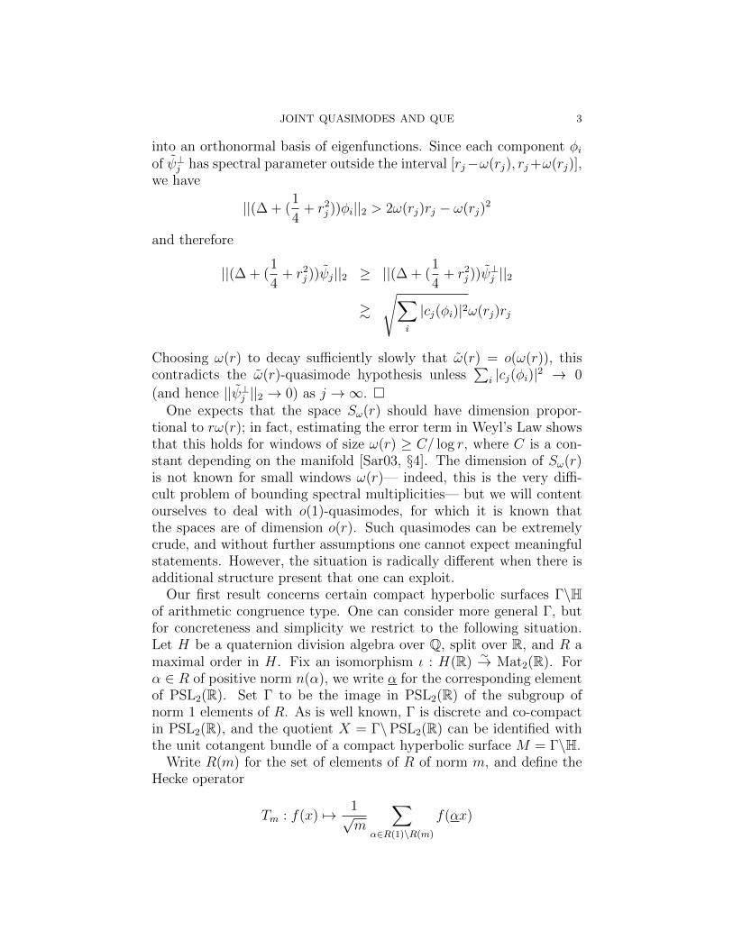
into an orthonormal basis of eigenfunctions. Since each component φiof ψ⊥j has spectral parameter outside the interval [rj−ω(rj), rj+ω(rj)],we have
||(∆ + (1
4+ r2j ))φi||2 > 2ω(rj)rj − ω(rj)
2
and therefore
||(∆ + (1
4+ r2j ))ψj||2 ≥ ||(∆ + (
1
4+ r2j ))ψ
⊥j ||2
&
√∑i
|cj(φi)|2ω(rj)rj
Choosing ω(r) to decay sufficiently slowly that ω(r) = o(ω(r)), thiscontradicts the ω(r)-quasimode hypothesis unless
∑i |cj(φi)|2 → 0
(and hence ||ψ⊥j ||2 → 0) as j →∞. One expects that the space Sω(r) should have dimension propor-
tional to rω(r); in fact, estimating the error term in Weyl’s Law showsthat this holds for windows of size ω(r) ≥ C/ log r, where C is a con-stant depending on the manifold [Sar03, §4]. The dimension of Sω(r)is not known for small windows ω(r)— indeed, this is the very diffi-cult problem of bounding spectral multiplicities— but we will contentourselves to deal with o(1)-quasimodes, for which it is known thatthe spaces are of dimension o(r). Such quasimodes can be extremelycrude, and without further assumptions one cannot expect meaningfulstatements. However, the situation is radically different when there isadditional structure present that one can exploit.
Our first result concerns certain compact hyperbolic surfaces Γ\Hof arithmetic congruence type. One can consider more general Γ, butfor concreteness and simplicity we restrict to the following situation.Let H be a quaternion division algebra over Q, split over R, and R amaximal order in H. Fix an isomorphism ι : H(R)
∼→ Mat2(R). Forα ∈ R of positive norm n(α), we write α for the corresponding elementof PSL2(R). Set Γ to be the image in PSL2(R) of the subgroup ofnorm 1 elements of R. As is well known, Γ is discrete and co-compactin PSL2(R), and the quotient X = Γ\PSL2(R) can be identified withthe unit cotangent bundle of a compact hyperbolic surface M = Γ\H.
Write R(m) for the set of elements of R of norm m, and define theHecke operator
Tm : f(x) 7→ 1√m
∑α∈R(1)\R(m)
f(αx)
4 SHIMON BROOKS AND ELON LINDENSTRAUSS
as the operator averaging over the Hecke points
Tm(x) = αx : α ∈ R(1)\R(m);
note that these formulas make sense both for x ∈ Γ\H and x ∈Γ\PSL2(R).
Our methods are reliant only on the Laplacian and a single Heckeoperator, and so we will be interested in the case where m = pk arepowers of a fixed prime p. It is well known that Tpk is a polynomial inTp; so in particular, eigenfunctions of Tp are eigenfunctions of all Tpk .It is known that for all but finitely many primes, the points Tpk(x) forma p+ 1-regular tree as k runs from 0 to ∞; we will always assume thatp is such a prime. We denote by Spk the sphere of radius k in this tree,given by Hecke points corresponding to the primitive elements of R ofnorm pk.
Since each α acts by isometries on Γ\H, the operator Tp commuteswith ∆. The spectrum of Tp on L2(Γ\H) lies in [−p+1√
p, p+1√
p], and since Tp
commutes with ∆, there is an orthonormal basis of L2(Γ\H) consistingof joint eigenfunctions for Tp and ∆. An ω-quasimode for Tp of approx-imate eigenvalue λ is a function ψ satisfying ||(Tp−λ)ψ||2 ≤ ω||ψ||2; wecall ψj∞j=1 a sequence of o(1)-quasimodes for Tp if each ψj is anωj-quasimode for Tp, and ωj → 0 as j →∞. As above in Lemma 1.1,for our purposes we may as well assume that each ωj-quasimode is alinear combination of eigenfunctions whose eigenvalues lie in intervalsof the form [λj − ωj, λj + ωj], for some sequence ωj → 0.
For any sequence φj of o(1)-quasimodes of the Laplacian ∆ on M ,normalized by ||φj||2 = 1, there exists a measure µj on S∗M (which weview as a probability measure on Γ\PSL2(R)), called the microlocallift of φj. This measure is asymptotically invariant under the geo-desic flow as the approximate eigenvalue of φj tends to infinity, andits projection to M is asymptotic to |φj|2darea. Since the space ofprobability measures on M is weak-* compact, we consider weak-*limit points of these microlocal lifts, called semiclassical measuresor quantum limits. The QUE problem asks whether such a limitpoint must be the uniform measure on S∗M . We shall use a version ofthe construction of these lifts due to Wolpert [Wol01] (this version isthe one used in [Lin01,Lin06]), where µj = |Φj|2dvol for suitably cho-sen Φj ∈ L2(S∗M); see Section 2. The construction satisfies that Φj isan eigenfunction of Tp when φj is, of the same eigenvalue; more gener-ally, applying this to each spectral component, Φj is an ωj-quasimodefor Tp whenever φj is, with the same approximate eigenvalue. Since
JOINT QUASIMODES AND QUE 5
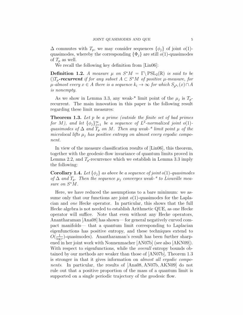
∆ commutes with Tp, we may consider sequences φj of joint o(1)-quasimodes, whereby the corresponding Φj are still o(1)-quasimodesof Tp as well.
We recall the following key definition from [Lin06]:
Definition 1.2. A measure µ on S∗M = Γ\PSL2(R) is said to be()Tp-recurrent if for any subset A ⊂ S∗M of positive µ-measure, forµ-almost every x ∈ A there is a sequence ki →∞ for which Spki (x)∩Ais nonempty.
As we show in Lemma 3.3, any weak-* limit point of the µj is Tp-recurrent. The main innovation in this paper is the following resultregarding these limit measures:
Theorem 1.3. Let p be a prime (outside the finite set of bad primesfor M), and let φj∞j=1 be a sequence of L2-normalized joint o(1)-quasimodes of ∆ and Tp on M . Then any weak-* limit point µ of themicrolocal lifts µj has positive entropy on almost every ergodic compo-nent.
In view of the measure classification results of [Lin06], this theorem,together with the geodesic-flow invariance of quantum limits proved inLemma 2.2, and Tp-recurrence which we establish in Lemma 3.3 implythe following:
Corollary 1.4. Let φj as above be a sequence of joint o(1)-quasimodesof ∆ and Tp. Then the sequence µj converges weak-* to Liouville mea-sure on S∗M .
Here, we have reduced the assumptions to a bare minimum: we as-sume only that our functions are joint o(1)-quasimodes for the Lapla-cian and one Hecke operator. In particular, this shows that the fullHecke algebra is not needed to establish Arithmetic QUE, as one Heckeoperator will suffice. Note that even without any Hecke operators,Anantharaman [Ana08] has shown— for general negatively curved com-pact manifolds— that a quantum limit corresponding to Laplacianeigenfunctions has positive entropy, and these techniques extend toO( 1
log r)-quasimodes). Anantharaman’s result has been further sharp-
ened in her joint work with Nonnenmacher [AN07b] (see also [AKN09]).With respect to eigenfunctions, while the overall entropy bounds ob-tained by our methods are weaker than those of [AN07b], Theorem 1.3is stronger in that it gives information on almost all ergodic compo-nents. In particular, the results of [Ana08, AN07b, AKN09] do notrule out that a positive proportion of the mass of a quantum limit issupported on a single periodic trajectory of the geodesic flow.
6 SHIMON BROOKS AND ELON LINDENSTRAUSS
Our results go further by allowing o(1)-quasimodes— which may betaken from rather large subspaces whose dimension is only boundedby o(r). In the paper [Bro11] the first named author shows that thesesubspaces are “optimally degenerate” for QUE, in the sense that givenany sequence of crj-dimensional subspaces Sc(rj) of the spaces SC(rj),
there exists a sequence ψj ∈ Sc(rj)∞j=1 such that the correspondingmicrolocal lifts do not converge to Liouville measure on S∗M— indeed,any weak-* limit point of these microlocal lifts must concentrate apositive proportion of its mass on a codimension 1 subset! Thus, ourjoint o(1)-quasimodes form spaces of largest-possible dimension thatcan satisfy QUE.
It should be remarked that these subspaces are considerably largerthan the spaces of Laplace-quasimodes that are expected to satisfyQUE without any Hecke assumption. This is a testament to the rigidityimposed by the additional structure of the Hecke correspondence, asalready apparent in [Lin06].
It is worth remarking here that the phrase “joint o(1)-quasimodes”can be misleading: the two orders of approximation are not necessarilythe same, and serve completely separate purposes; the approximationto the Laplace eigenvalue is used to guarantee asymptotic invarianceunder the geodesic flow, while the approximation to the Hecke eigen-value is used to establish positive entropy on almost every ergodic com-ponent and Tp-recurrence.
Our methods also apply to the case of M = Γ\H × H, with Γ aco-compact, irreducible lattice in PSL(2,R) × PSL(2,R). Here we donot assume any Hecke structure1; instead, we take the sequence φjto consist of joint o(1)-quasimodes of the two partial Laplacians, eachon the respective copy of H. The Laplacian on M is the sum of the twopartial Laplacians, and so the large eigenvalue limit for the Laplacianentails at least one of the two partial eigenvalues going to infinity (afterpassing to a subsequence, if necessary). At present, we have been ableto apply our methods only to the case where one partial eigenvalue(say the second) remains bounded, and the other tends to ∞.
By the arguments of [Lin01] and Section 2.4, this means that themicrolocal lift to Γ\PSL(2,R)×H becomes invariant under the actionof the diagonal subgroup A of PSL(2,R) acting on the first coordinate.By applying the methods of Theorem 1.3 to use the foliation given byvarying the second coordinate in an analogous way to use of the Hecke
1By Margulis’ Arithmeticity Theorem such lattices are necessarily arithmetic,though it is not known if they are necessarily of congruence type (which is necessaryfor the existence of Hecke operators with good properties).
JOINT QUASIMODES AND QUE 7
Correspondence Tp for congruence surfaces, we are able to prove thatany quantum limit of such a sequence must also carry positive entropyon a.e. ergodic component (with respect to the A-action on the firstcoordinate). Thus, [Lin06, Thm. 1.1] in conjunction with the relevantrecurrence property proved in Lemma 5.6 again may be used to showequidistribution of |φj|2dvol as well as their microlocal lifts:
Theorem 1.5. Let φj be a sequence of joint o(1)-quasimodes of ∆1
and ∆2 on Γ\H × H with approximate spectral parameters r1j , r2j and
where Γ is an irreducible cocompact lattice in PSL(2,R) × PSL(2,R).Assume r1j → ∞ and r2j bounded. Then the sequence of lifts µj of
|φj|2 dvol to Γ\PSL(2,R)×H converges weak-* to the uniform measureon Γ\PSL(2,R)×H.
The argument is analogous to the one presented here for the rank-onearithmetic case in Theorem 1.3, and we present the necessary modifi-cations of the argument in section 5.
The results of [BL03], along with an appropriate construction ofmicrolocal lifts, were generalized by Silberman and Venkatesh [SV07,SV10] who, using the measure classification results of [EKL06], wereable to extend the QUE results of [Lin06] to quotients of more generalsymmetric spaces (they also had to develop an appropriate microlocallift). It is likely possible to extend the techniques of this paper to theircontext. We also hope that our work may be extended to the case ofΓ\H×H where both partial eigenvalues are growing to ∞.
Regarding finite volume arithmetic surfaces such as SL(2,Z)\H, itwas shown in [Lin06] that any quantum limit has to be a scalar mul-tiple of the Liouville measure— though not necessarily with the rightscalar— and similar results can be provided by our techniques usinga single Hecke operator. Recently, Soundararajan [Sou10] has givenan elegant argument that settles this escape of mass problem for jointeigenfunctions of the full Hecke algebra and (in view of the results of[Lin06]) shows that the only quantum limit is the normalized Liouvillemeasure. An interesting open question is whether our p-adic wave equa-tion techniques can be used to rule out escape of mass using a singleHecke operator. We also mention that Holowinsky and Soundararajan[HS10] have recently developed an alternative approach to establishingArithmetic Quantum Unique Ergodicity for joint eigenfunctions of allHecke operators. This approach requires a cusp, and is only applica-ble in cases where the Ramanujan Conjecture holds; this conjecture isopen for the Hecke-Maass forms, but has been established by Delignefor holomorphic cusp forms — a case which our approach does nothandle.
8 SHIMON BROOKS AND ELON LINDENSTRAUSS
Acknowledgments. We thank Peter Sarnak for helpful discussions,and Shahar Mozes for helpful suggestions that simplified the proof ofLemma 5.4.
2. Microlocal Lifts of Quasimodes
2.1. Some Harmonic Analysis on PSL(2,R). We begin by review-ing some harmonic analysis on PSL(2,R) that we will need. Through-out, we write X = Γ\PSL(2,R) and M = Γ\H = Γ\PSL(2,R)/K,where K = SO(2) is the maximal compact subgroup.
Fix an orthonormal basis φj of L2(M) consisting of Laplace eigen-functions, which we can take to be real-valued for simplicity. Eacheigenfunction generates, under right translations, an irreducible repre-sentation Vj = φj(xg−1) : g ∈ PSL(2,R) of PSL(2,R), which span adense subspace of L2(X).
We distinguish the pairwise orthogonal weight spaces A2n in eachrepresentation, consisting of those functions satisfying f(xkθ) = ei2nθf(x)
for all kθ =
(cos θ sin θ− sin θ cos θ
)∈ K and x ∈ X. The weight spaces to-
gether span a dense subspace of Vj. Each is one-dimensional in Vj,
spanned by φ(j)2n where
φ(j)0 = φj ∈ A0
(irj +1
2+ n)φ
(j)2n+2 = E+φ
(j)2n
(irj +1
2− n)φ
(j)2n−2 = E−φ
(j)2n
Here E+ and E− are the raising and lowering operators, first-
order differential operators corresponding to
(1 ii −1
)∈ sl(2,C) and(
1 −i−i −1
)∈ sl(2,C) in the complexified Lie algebra. The normal-
ization is such that each φ(j)2n is a unit vector. Continuing with the
identification of the elements in (2,C) with first order invariant differ-ential operators on X, we also make use of the following operators
H =
(1 00 −1
)W =
(0 −11 0
)X+ =
(0 10 0
)
JOINT QUASIMODES AND QUE 9
note that H is the derivative in the geodesic-flow direction, W is thederivative in the fibre K direction, and X+ is the derivative in thestable horocycle direction. We will also need the second order operator
Ω = 12(E+E− + E−E+) +
W 2
4
which commutes with all the invariant differential operators on X andagrees with ∆ on the space of K-invariant functions.
It is easy to check that the distribution
Φ(j)∞ =
∞∑n=−∞
φ(j)2n
satisfies HΦ(j)∞ = (irj − 1
2)Φ
(j)∞ and X+Φ
(j)∞ = 0. We also record the
identities
H =1
2(E+ + E−)
E+Φ(j)∞ = (irj −
1
2− i
2W )Φ(j)
∞
E−Φ(j)∞ = (irj −
1
2+i
2W )Φ(j)
∞
E+E−Φ(j)∞ = −(r2j +
1
4)Φ(j)∞ + (
1
4W 2 − i
2W )Φ(j)
∞
E+E−φ(j)0 = −(r2j +
1
4)φ
(j)0 = ∆φ
(j)0(2.1)
2.2. Construction of the Microlocal Lift. For any ω(r)-quasimodeφ, with approximate Laplace eigenvalue 1
4+ r2, we seek a smooth func-
tion Φ on Γ\PSL(2,R) satisfying:
(Φ1) The measure |Φ|2dvol is asymptotic to the distribution definedby
f 7→ 〈Op(f)φ, φ〉L2(M) = 〈fΦ∞, φ〉L2(X)
In particular, the projection of the measure |Φ|2dvol on X to M
is asymptotic to |φ|2darea; i.e., for any smooth f ∈ C∞(M), wehave ∫
X
f |Φ|2dvol ∼∫M
f |φ|2darea
as r → ∞. It is in this sense that |Φ|2dvol “lifts” the measure|φ|2darea to X.
10 SHIMON BROOKS AND ELON LINDENSTRAUSS
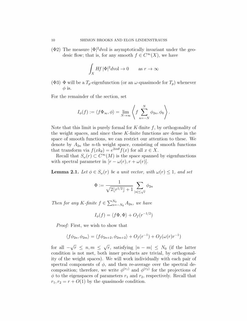
(Φ2) The measure |Φ|2dvol is asymptotically invariant under the geo-desic flow; that is, for any smooth f ∈ C∞(X), we have∫
X
Hf |Φ|2dvol→ 0 as r →∞
(Φ3) Φ will be a Tp-eigenfunction (or an ω-quasimode for Tp) wheneverφ is.
For the remainder of the section, set
Iφ(f) := 〈fΦ∞, φ〉 = limN→∞
⟨f
N∑n=−N
φ2n, φ0
⟩.
Note that this limit is purely formal for K-finite f , by orthogonality ofthe weight spaces, and since these K-finite functions are dense in thespace of smooth functions, we can restrict our attention to these. Wedenote by A2n the n-th weight space, consisting of smooth functionsthat transform via f(xkθ) = e2inθf(x) for all x ∈ X.
Recall that Sω(r) ⊂ C∞(M) is the space spanned by eigenfunctionswith spectral parameter in [r − ω(r), r + ω(r)].
Lemma 2.1. Let φ ∈ Sω(r) be a unit vector, with ω(r) ≤ 1, and set
condition is not met, both inner products are trivial, by orthogonal-ity of the weight spaces). We will work individually with each pair ofspectral components of φ, and then re-average over the spectral de-composition; therefore, we write φ(r1) and φ(r2) for the projections ofφ to the eigenspaces of parameters r1 and r2, respectively. Recall thatr1, r2 = r +O(1) by the quasimode condition.
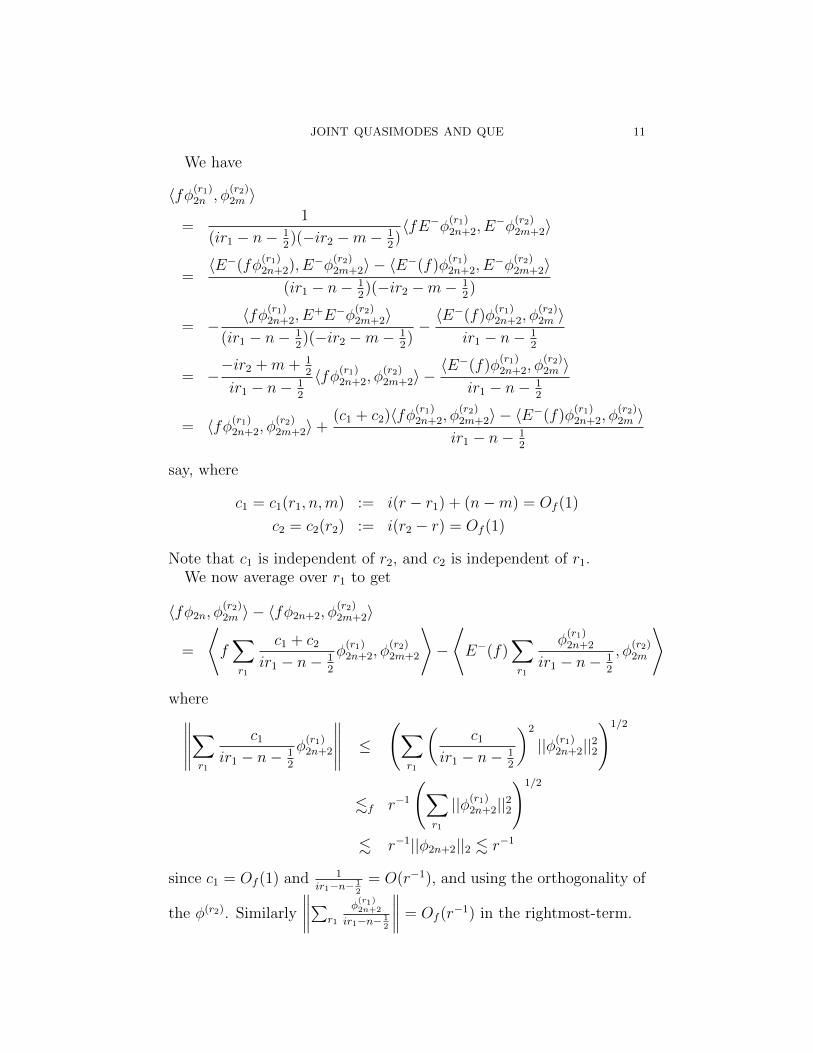
JOINT QUASIMODES AND QUE 11
We have
〈fφ(r1)2n , φ
(r2)2m 〉
=1
(ir1 − n− 12)(−ir2 −m− 1
2)〈fE−φ(r1)
2n+2, E−φ
(r2)2m+2〉
=〈E−(fφ
(r1)2n+2), E
−φ(r2)2m+2〉 − 〈E−(f)φ
(r1)2n+2, E
−φ(r2)2m+2〉
(ir1 − n− 12)(−ir2 −m− 1
2)
= −〈fφ(r1)
2n+2, E+E−φ
(r2)2m+2〉
(ir1 − n− 12)(−ir2 −m− 1
2)−〈E−(f)φ
(r1)2n+2, φ
(r2)2m 〉
ir1 − n− 12
= −−ir2 +m+ 1
2
ir1 − n− 12
〈fφ(r1)2n+2, φ
(r2)2m+2〉 −
〈E−(f)φ(r1)2n+2, φ
(r2)2m 〉
ir1 − n− 12
= 〈fφ(r1)2n+2, φ
(r2)2m+2〉+
(c1 + c2)〈fφ(r1)2n+2, φ
(r2)2m+2〉 − 〈E−(f)φ
(r1)2n+2, φ
(r2)2m 〉
ir1 − n− 12
say, where
c1 = c1(r1, n,m) := i(r − r1) + (n−m) = Of (1)
c2 = c2(r2) := i(r2 − r) = Of (1)
Note that c1 is independent of r2, and c2 is independent of r1.We now average over r1 to get
〈fφ2n, φ(r2)2m 〉 − 〈fφ2n+2, φ
(r2)2m+2〉
=
⟨f∑r1
c1 + c2ir1 − n− 1
2
φ(r1)2n+2, φ
(r2)2m+2
⟩−
⟨E−(f)
∑r1
φ(r1)2n+2
ir1 − n− 12
, φ(r2)2m
⟩
where∥∥∥∥∥∑r1
c1ir1 − n− 1
2
φ(r1)2n+2
∥∥∥∥∥ ≤
(∑r1
(c1
ir1 − n− 12
)2
||φ(r1)2n+2||22
)1/2
.f r−1
(∑r1
||φ(r1)2n+2||22
)1/2
. r−1||φ2n+2||2 . r−1
since c1 = Of (1) and 1ir1−n− 1
2
= O(r−1), and using the orthogonality of
the φ(r2). Similarly
∥∥∥∥∑r1
φ(r1)2n+2
ir1−n− 12
∥∥∥∥ = Of (r−1) in the rightmost-term.
12 SHIMON BROOKS AND ELON LINDENSTRAUSS
Thus, further averaging over r2 and applying Cauchy-Schwarz gives
〈fφ2n, φ2m〉 − 〈fφ2n+2, φ2m+2〉
=∑r2
⟨f∑r1
c1 + c2ir1 − n− 1
2
φ(r1)2n+2, φ
(r2)2m+2
⟩−
⟨E−(f)
∑r1
φ(r1)2n+2
ir1 − n− 12
, φ2m
⟩
≤ Of (r−1) +
∑r2
⟨f∑r1
c2ir1 − n− 1
2
φ(r1)2n+2, φ
(r2)2m+2
⟩+Of (r
−1)
≤
⟨f∑r1
1
ir1 − n− 12
φ(r1)2n+2,
∑r2
c2φ(r2)2m+2
⟩+Of (r
−1)
≤ ||f ||∞ ·
∥∥∥∥∥∑r1
1
ir1 − n− 12
φ(r1)2n+2
∥∥∥∥∥ ·∥∥∥∥∥∑
r2
c2φ(r2)2m+2
∥∥∥∥∥+Of (r−1)
.f r−1
using again the orthogonality of the φ(r), and the fact that c2 = Of (1).Therefore we finally arrive at
〈fφ2n, φ2m〉 = 〈fφ2n+2, φ2m+2〉+Of (r−1)
We iterate this |m| ≤√r times, arriving at
〈fφ2n, φ2m〉 = 〈fφ2(n−m), φ0〉+Of (√rr−1)
Now, by definition
〈fΦ,Φ〉 =1
2br1/2c+ 1
∑|m|,|n|≤
√r
〈fφ2n, φ2m〉
and so we now combine all weight space components together to get
〈fΦ,Φ〉 =
N0∑n=−N0
(2br1/2c − 2|n|+ 1)
(2br1/2c+ 1)〈fφ2n, φ0〉+Of (
√rr−1)
Since for all |n| ≤ N0
2br1/2c − 2|n|+ 1
2br1/2c+ 1= 1 +Of (r
−1/2)
and using the K-finiteness of f , we see that
〈fΦ,Φ〉 =∑n
〈fφ2n, φ0〉+Of (r−1/2) +Of (
√rr−1)
as required. For any given sequence φj of quasimodes, we have constructed a
sequence Φj∞j=1 such that the microlocal lifts |Φj|2dvol are positive
JOINT QUASIMODES AND QUE 13
measures, asymptotically equivalent to the distributions Iφj . Moreover,since Φj are constructed from φj via left-invariant operators, and Tpacts by isometries on the left, this construction is equivariant withrespect to the action of Tp, and Φj will be a Tp-eigenfunction (resp.ωj-quasimode for Tp) whenever φj is.
2.3. Asymptotic Invariance under the Geodesic Flow. We nowturn to the invariance under the geodesic flow. By Lemma 2.1, we mayconsider the distribution
f 7→ 〈fΦ∞, φ〉in place of our positive-measure microlocal lift, since it is more amenableto verifying this invariance.
Lemma 2.2. Let φj be a sequence of ω(rj) quasimodes with approx-imate parameter rj, satisfying rj → ∞ and ω(rj) → 0. Then for anyf ∈ C∞(S∗M), we have Iφj(Hf)→ 0 as rj →∞.
Remark: In contrast with Lemma 2.1, here it is necessary to assumethat ω(rj) → 0; in fact, the sequences of quasimodes considered in[Bro11] have ω(rj) 1, and do not satisfy Lemma 2.2.
Proof: Once again, we may assume that f ∈∑N0
n=−N0A2n is K-
finite, and it will be natural to consider the contribution of each pairof spectral parameters individually; so we again write φ(r1) and φ(r2)
for the projections of φ to the eigenspaces of parameters r1 and r2respectively, and similarly Φ
where D1(W ) is a differential operator in W . This means, after inte-grations by parts in W (recalling that Wφ(r2) = 0) we get
−(r22 +1
4)〈fΦ(r1)
∞ , φ(r2)〉
= −(r21 +1
4)〈fΦ(r1)
∞ , φ(r2)〉+ 2ir1〈HfΦ(r1)∞ , φ(r2)〉+ 〈(D2f)Φ(r1)
∞ , φ(r2)〉
14 SHIMON BROOKS AND ELON LINDENSTRAUSS
for a fixed differential operator D2. But since r1, r2 = r + o(1), wehave r21− r22 = o(r), and so putting all of the spectral components backtogether again we see
(r21 − r22)〈fΦ(r1)∞ , φ(r2)〉 = 2ir1〈(Hf)Φ(r1)
∞ , φ(r2)〉+ 〈(D2f)Φ(r1)∞ , φ(r2)〉
(r21 − r22)〈fΦ(r1)N0, φ(r2)〉 = 2ir1〈(Hf)Φ(r1)
∞ , φ(r2)〉+ 〈(D2f)Φ(r1)∞ , φ(r2)〉
o(r)||f ||∞||ΦN0||2||φ||2 = 2ir〈(Hf)Φ∞, φ〉+ of (1)||ΦN0+1||2 + Iφ(D2f)
of (r) = 2irIφ(Hf) + of (1) +Of (1)
where we may replace Φ∞ on the left with ΦN0 , the projection of Φ∞to∑|n|≤N0
An, by orthogonality of weight spaces— and similarly on
the right side since f ∈∑|n|≤N0
An implies that Hf ∈∑|n|≤N0+1An—
noting that ||ΦN0||2 =√
2N0 + 1 = Of (1) and similarly ||ΦN0+1||2 =Of (1).
The result now follows by dividing by r and taking the limit asj →∞.
2.4. Microlocal lift on Γ\H×H. Given a quasimode φ on Γ\H, weconstructed an element Φ ∈ L2 (Γ\PSL(2,R)) satisfying (Φ1)–(Φ3)on p. 9 by considering φ as a right K = SO(2)-invariant function onΓ\PSL(2,R) and applying a carefully chosen generalized differential
operator of the type D =∑k
i=1 fi(Ω)Xi with fi appropriately chosenanalytic functions, Ω the Casimir operator and Xi some invariant dif-ferential operators on Γ\PSL(2,R). We note that the choice of Ddepends on the approximate eigenvalue of φ. Since Ω is in the center ofthe algebra of invariant differential operators it is easy to make sensevery concretely of the operator D by decomposing L2(Γ\PSL(2,R))to ω-eigenspaces and applying — on the eigenspace corresponding toeigenvalue r —the honest differential operator
∑ki=1 fi(r)Xi.
Now suppose that we are working not on Γ\H, but on X = Γ\H×H,with Γ an irreducible lattice in PSL(2,R) × PSL(2,R). Suppose ∆1
is the Laplacian operator acting on the first H component, and ∆2
the Laplacian on the second such component. If φ is an approximateeigenfunction of both ∆1 and ∆2 with approximate eigenvalues r1, r2with r1 large, we could take the same generalized differential operatorD discussed in the previous paragraph and consider it as an operatoron Γ\PSL(2,R) × H. Then if φ is considered as a SO(2)-invariantfunction on Γ\PSL(2,R) × H, taking Φ = Dφ we obtain a functionsatisfying the analogous conditions to (Φ1)–(Φ3) for Γ\PSL(2,R)×Has explained in greater detail in [Lin01].
JOINT QUASIMODES AND QUE 15
3. The Propagation Lemma
Our methods were inspired in part by the work of Anantharaman et.al. (eg., [Ana08,AN07b,AKN09,Riv10b,Riv10]); in particular, the ob-servation that one can obtain interesting information on eigenfunctions—and quasimodes— by breaking the function up into smaller pieces, let-ting each piece disperse individually through the quantum dynamics,and adding the pieces back together. In this spirit, our approach isto use an analogous “wave propagation” on the Hecke tree to dispersepieces of our Tp-quasimodes, as described in Lemma 3.2. As will be-come clear later on, this dispersion alone is not enough to get Theo-rem 1.3; we will need to employ interferences in order to build a betterdispersion mechanism, that amplifies a desired spectral window.
3.1. Constructing the Kernel. The following lemma proved alongthe lines of [BL11] is central to our approach:
Lemma 3.1. Let 0 < η < 1/2. For any sufficiently large N ∈ N(depending on η), and any θ0 ∈ [0, π], there exists an operator KN onS∗M satisfying:
(1) KN(δx) is supported on the union of Hecke points y ∈ Tpj(x) up todistance j ≤ N in the Hecke tree.
(2) KN has matrix coefficients bounded by O(p−Nδ), in the sense thatfor any x ∈ S∗M
|KN(f)(x)| . p−NδN∑j=0
∑y∈S
pj(x)
|f(y)|
where δ depends only on η (explicitly, can be taken to be η2/512).(3) Any Tp eigenfunction is also an eigenfunction of KN with eigen-
value ≥ −1.(4) Eigenfunctions with Tp-eigenvalue 2 cos θ with |θ − θ0| ≤ 1
2N, as
well as all untempered eigenfunctions (Tp-eigenvalue 6∈ [−2, 2]) haveKN -eigenvalue > η−1.
Lemma 3.1 is based on the well known connection between Heckeoperators and Chebyshev polynomials. A way to derive these whichwe have found appealing is via the following p-adic wave equation for,say, compactly supported functions on Tp+1 :
Φn+1 =1
2TpΦn −
(1−
T 2p
4
)Ψn
Ψn+1 =1
2TpΨn + Φn
16 SHIMON BROOKS AND ELON LINDENSTRAUSS
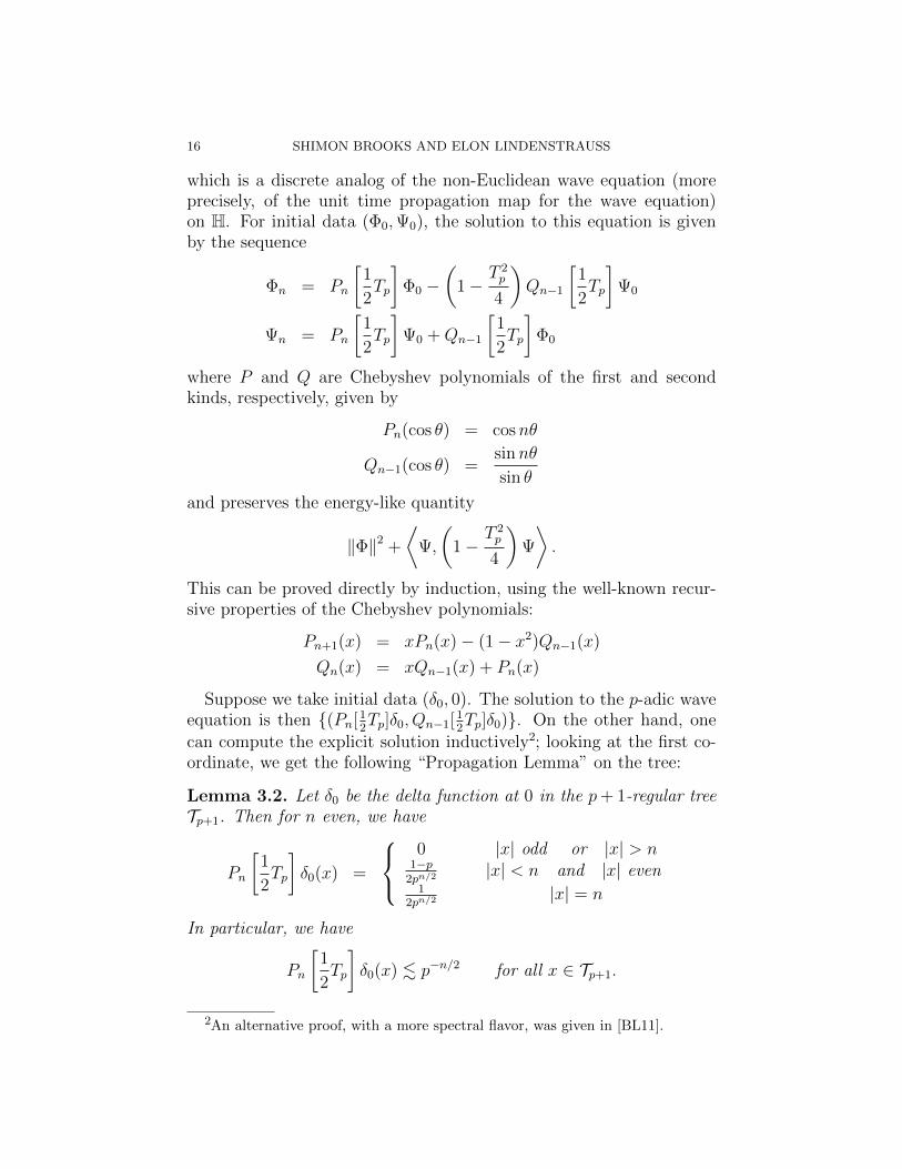
which is a discrete analog of the non-Euclidean wave equation (moreprecisely, of the unit time propagation map for the wave equation)on H. For initial data (Φ0,Ψ0), the solution to this equation is givenby the sequence
Φn = Pn
[1
2Tp
]Φ0 −
(1−
T 2p
4
)Qn−1
[1
2Tp
]Ψ0
Ψn = Pn
[1
2Tp
]Ψ0 +Qn−1
[1
2Tp
]Φ0
where P and Q are Chebyshev polynomials of the first and secondkinds, respectively, given by
Pn(cos θ) = cosnθ
Qn−1(cos θ) =sinnθ
sin θ
and preserves the energy-like quantity
‖Φ‖2 +
⟨Ψ,
(1−
T 2p
4
)Ψ
⟩.
This can be proved directly by induction, using the well-known recur-sive properties of the Chebyshev polynomials:
Pn+1(x) = xPn(x)− (1− x2)Qn−1(x)
Qn(x) = xQn−1(x) + Pn(x)
Suppose we take initial data (δ0, 0). The solution to the p-adic waveequation is then (Pn[1
2Tp]δ0, Qn−1[
12Tp]δ0). On the other hand, one
can compute the explicit solution inductively2; looking at the first co-ordinate, we get the following “Propagation Lemma” on the tree:
Lemma 3.2. Let δ0 be the delta function at 0 in the p+ 1-regular treeTp+1. Then for n even, we have
Pn
[1
2Tp
]δ0(x) =
0 |x| odd or |x| > n
1−p2pn/2 |x| < n and |x| even
12pn/2 |x| = n
In particular, we have
Pn
[1
2Tp
]δ0(x) . p−n/2 for all x ∈ Tp+1.
2An alternative proof, with a more spectral flavor, was given in [BL11].
JOINT QUASIMODES AND QUE 17
We now have a description of the p-adic wave propagation in bothspectral and spacial terms, which we will use to construct our desiredradial kernel KN on the Hecke tree. It will be convenient to parametrizethe Tp-eigenvalues as 2 cos(θ), where
• The tempered spectrum is parametrized by θ ∈ [0, π].• The positive part of the untempered spectrum has iθ ∈ (0, log
√p).
• The negative part of the untempered spectrum has iθ + π ∈(0, log
√p).
We also recall that for any (say, compactly supported) radial kernel kon Tp+1, any Tp-eigenfunction φ is also an eigenfunction of convolutionwith k, with eigenvalue— depending only on the Tp-eigenvalue of φ—given by the spherical transform hk(θ).
Now, Lemma 3.2 is a good start towards Lemma 3.1, since the kernelPn[1
2Tp]δ0 satisfies the first two properties of Lemma 3.1, with δ = 1/2.
Unfortunately, the spherical transform of this kernel is 2 cosnθ, whichis bounded by 2 and cannot satisfy the third condition of Lemma 3.1.More crucially, it takes negative values that are as large in absolutevalue as the maximum. In order to create the kernel we want, we willhave to combine different Pn[1
2Tp]δ0 waves together, in such a way that
they interfere constructively at our chosen spectral interval, to generatea large eigenvalue there, but do not become too negative elsewhere.To allow this kind of interference, however, we will have to sacrificesomewhat in our bounds for δ.
Proof of Lemma 3.1. The case where θ0 = 0 is a bit simpler, so weconsider this case first. Using the Hecke correspondence, we can as-sign to any “kernel” (spherically invariant compactly supported func-tion) on a p + 1-regular tree with a marked point an operator onL2(S∗M). We will produce the operator KN satisfying the proper-ties of Lemma 3.1 from such a kernel kN , which in turn will be definedfrom its spherical transform hkN . Denoting the Fejer kernel of order L
by FL(θ) = 1L
(sin(Lθ/2)sin(θ/2)
)2, we will set the spherical transform to be
hkN (θ) = FL(qθ)− 1
for an appropriately chosen q. Now FL & L on (− 1L, 1L
), which containsthe spectral parameters for components of Φj if N ≥ L, and FL isnon-negative, so the third condition of Lemma 3.1 is satisfied on thetempered spectrum, as long as N > L > η−1 + 1. Moreover, we canwrite
FL(qθ)− 1 =L∑j=1
2(L− j)L
cos (jqθ)
18 SHIMON BROOKS AND ELON LINDENSTRAUSS
and observing that cos(jqθ) > cos(0) on the entire untempered spec-trum as long as q is even, we see that the third condition holds on thefull spectrum. We also observe that
|kN(x)| ≤L∑j=1
2
∣∣∣∣Pjq [1
2Tp
]δ0
∣∣∣∣.
L∑j=1
p−jq/2
. p−q/2
which provides the second condition of Lemma 3.1, as long as q ≥ 2Nδ.Moreover, since each Pjq[
12Tp]δ0 vanishes outside the ball of radius Lq,
the first condition is satisfied whenever Lq ≤ N . So we may takeL = dη−1e + 1, and q = 2bN/2Lc, which yields δ = bq/2Nc & η. Thesame kernel also works for θ = π and the untempered spectrum.
We must now consider the case of θ0 ∈ (0, π). The general idea isthe same, but in order to maintain positivity on the untempered spec-trum, we can’t simply shift the Fejer kernel to a different approximateeigenvalue. The solution to this problem is to find a suitable multipleof θ0, which is sufficiently close to 0, and choose our value of q to bedivisible by this multiple. Thus the original Fejer kernel evaluated atqθ0 will still be large, as before, without affecting its positivity on theuntempered spectrum. To guarantee that we can find such a suitablevalue of q, we will invoke Dirichlet’s Theorem on Diophantine approxi-mation. We will lose some in our bounds for δ (as well as in the impliedconstant)— whereas our previous argument gave δ & η, we will haveto settle for a more modest δ & η2 in order to achieve the necessaryflexibility in choosing q . The following argument is essentially identicalto the one appearing in [BL11], with some tweaking to the constantsto accommodate our quasimodes.
Set L = bη−1c and Q = d18Nηe. By Dirichlet’s Theorem, we can
find a positive integer q ≤ Q such that |qθ0 mod 2π| < 2πQ−1. Thereexists an even multiple of q, say q′ = 2lq, such that 1
64Qη ≤ q′ ≤ 2Q
— indeed, if q ≥ 1128Qη, we can simply take l = 1; otherwise there is
a multiple of q between 1128Qη and 1
64Qη, so take twice that multiple.
Either way, since N is assumed to be large depending on η, we mayassume Qη > 64 which implies that both when l = 1 and l > 1 we havethat
2l <1
32Qη and |q′θ0 mod 2π| < 1
16πη
JOINT QUASIMODES AND QUE 19
We now set the spherical transform of kN to be hkN (θ) = F2L(q′θ)− 1,where F2L is the Fejer kernel of order 2L, and KN the correspondingoperator on L2(S∗M) i.e.
KN =2L∑j=1
2L− jL
Pjq′
(Tp2
).
For any Tp-eigenfunction with eigenvalue 2 cos θ with θ ∈ [θ0 −12N−1, θ0 + 1
2N−1], we have that
|q′(θ0 − θ)| ≤ QN−1 ≤ η/8 + 1/N < η/6;
this means that
|q′θ mod 2π| < 1
16πη +
1
6η <
1
8πη ≤ π
8L.
It follows that
F2L(q′θ) =1
2L
sin2(Lq′θ)
sin2(q′θ/2)≥ 2
L
sin2(Lq′θ)
(q′θ)2
≥ 2L
(sin(Lq′θ)
Lq′θ
)2
But since L ∈ Z, and q′θ mod 2π ∈(− π
8L, π8L
), we have Lq′θ mod 2π ∈
[−π8, π8], which implies that∣∣∣∣sin(Lq′θ)
Lq′θ
∣∣∣∣ ≥ sin π4
π4
=1√2
4
π
whereby
F2L(q′θ) ≥ 2L
(1√2
4
π
)2
≥ 2L8
π2> L+ 1
as long as L ≥ 2 (which follows from the hypothesis η < 1/2). There-fore the KN -eigenvalue of this eigenfunction will be > L + 1 ≥ η−1.Moreover, since F2L is positive, the spherical transform of kN is boundedbelow by −1; note also that on the untempered spectrum of Tp, thenKN -eigenvalue is also > L + 1 . It remains to check the first twoproperties.
Now, by Lemma 3.2, we see that the kernel whose spherical transformis cos 2jθ— i.e., the kernel of P2j(
12Tp)— has sup-norm .p p−j. The
spherical transform of kN is a sum of terms of the form 2L−jL
cos jq′θ,
20 SHIMON BROOKS AND ELON LINDENSTRAUSS
where j = 1, 2, . . . , 2L (note that we eliminated the j = 0 term bysubtracting off the constant contribution to F2L) and q′ ∈ 2Z. Thus
||kN ||∞ .L∑j=1
p−jq′.p p
−q′
Then, since
q′ ≥ 1
64Qη ≥ 1
512Nη2
the second condition is satisfied with δ = 1512η2. Moreover, since each
kernel Pjq′(12Tp) is supported in a ball of radius jq′ ≤ 2L · 2Q < N , the
full kernel kN is supported in a ball of radius N . This concludes theproof of Lemma 3.1.
The kernel kN produced by Lemma 3.1 will be used in section 4 toestablish positive entropy on a.e. ergodic component of quantum limitsarising from joint o(1)-quasimodes. It will also be used in section 3.2,though in a less delicate way (in particular, without making use ofproperty (3) of Lemma 3.1).
3.2. Hecke Recurrence for Quasimodes. As shown in [Lin06] (andimplicitly already in [Lin01]) a quantum limit arising from a sequenceof Tp-eigenfunctions is Hecke recurrent. This remains true for Tp-quasi-modes, and in order to streamline the presentation we shall make useof the discussion in section 3.1. The recurrence property for quantumlimits arising from our joint o(1) quasimodes, follows immediately fromthe following estimate (see [Lin06] for details):
Lemma 3.3. Let Φj be a sequence of ωj-quasimodes for Tp, withωj → 0, such that the sequence |Φj|2dvol converges weak-* to a measureµ. Let x ∈ suppµ ⊂ S∗M , and B a small open ball around e ∈ G (say,of radius less than 1/3 the injectivity radius of S∗M). Then
lim infj→∞
∑dp(x,y)≤N
∫yB|Φj|2∫
xB|Φj|2
→∞ as N →∞
uniformly in x and the radius of B.
Here, dp(x, y) refers to distance in the Hecke tree containing x and y,i.e. the smallest d for which x ∈ Tpd(y); in particular, the sum is finite.While we have in mind the case where the Φj arise from a sequenceof joint ∆ and Tp quasimodes on M as in Lemma 2.1, the proof ofLemma 3.3 only uses the Tp-structure, and holds for any sequence ofo(1)-quasimodes for Tp on S∗M .
JOINT QUASIMODES AND QUE 21
Proof of Lemma 3.3. We will use a simplified version of the construc-tion in Lemma 3.1. Let L be a large integer. Suppose Φj is a ωj-quasimode for Tp with approximate eigenvalue λj and set θj ∈ [0, 2π]by
θj =
cos−1(λj/2) if λj ∈ [−2, 2]
0 if λj > 2
π if λj < −2
.
Find a q ∈ 1, . . . , 100L so that
(3.1) |qθj mod 2π| ≤ π
50L,
and set
K =L∑l=1
P2ql
(Tp2
).
By Lemma 3.2 and two consecutive applications of the Cauchy Schwarzinequality
|KΦj(x)| .
∣∣∣∣∣∣L∑l=1
∑y: 2q(l−1)<dp(y,x)≤2ql
p−2ql/2Φj(y)
∣∣∣∣∣∣≤
L∑l=1
(# y : 2q(l − 1) < dp(y, x) ≤ 2ql · p−2ql ·
∑y : 2q(l − 1) < dp(y, x) ≤ 2ql
|Φj(y)|2)1/2
.L∑l=1
( ∑y: 2q(l−1)<dp(y,x)≤2ql
|Φj(y)|2)1/2
≤
(L
∑dp(y, x) ≤ 100L2
|Φj(y)|2)1/2
.
and similarly for every g ∈ B
|KΦj(xg)| .
(L
∑dp(y, x) ≤ 100L2
|Φj(yg)|2)1/2
.
Set a =∑L
l=1 P2ql(λj/2) (which we can also write in the tempered
case as∑L
l=1 cos(2qlθj)); by considering separately the tempered anduntempered cases (using in the former case (3.1)) it can be verified thata & L. Since Φj is an ωj-quasimode
‖KΦj − aΦj‖ = OL(ωj).
22 SHIMON BROOKS AND ELON LINDENSTRAUSS
It follows that
a2∫xB
|Φj|2 ≤∫xB
|KΦj|2 +OL(ωj)vol(B)1/2
. L∑
dp(y,x)≤100L2
∫yB
|Φj|2 +OL(ωj)vol(B)1/2.
Since a2 & L2, ωj → 0, and x ∈ suppµ (so that lim infj→∞∫xB|Φj|2 >
We recall the setup, which is the same as in [RS94]: we begin witha quaternion division algebra
H(Q) = x+ iy + jz + ijw : x, y, z, w ∈ Qwith i2 = a, j2 = b, ij = −ji and the usual norm n(x+ iy+ jz+ ijw) =x2−ay2−bz2 +abw2 and trace tr(x+ iy+jz+ ijw) = 2x; that H(Q) isa division algebra is equivalent to n(α) 6= 0 for all nonzero α ∈ H(Q);we also assume a > 0 and then
ι(x+ iy + jz + ijw) =
(x+√ay z +
√aw
b(z −√aw) x−
√ay
)gives an embedding of H(Q) to Mat2(F ), F = Q(
√a), which extends
to an isomorphism of rings between H(R) to Mat2(R). An order R <H(Q) is a subring containing 1 which as an additive group is of rank4 and so that tr(α) ∈ Z for every α ∈ R. An example of an orderis R = OF + jOF (with F embedded in H(Q) in the obvious way).We take R to be a maximal order containing R; the assumptions that
JOINT QUASIMODES AND QUE 23
R is maximal is not important, but makes it easier to write thingsaccurately in classical language. Cf. [Eic65] for more details.
The following estimate can be derived using the techniques of [BL03],specifically Lemmas 3.1 and 3.3 there (much more general statementsof this type by Silberman and Venkatesh can be found in [SV10]). Weinclude the proof below for completeness.
Lemma 4.1. For τ fixed but small enough, there exists a constant c(depending only on τ), such that for any x, z ∈ X = Γ\PSL(2,R), andany ε < cp−2N , the tube zB(ε, τ) ⊂ X contains at most O(N) of theHecke points
⋃j≤N Tpj(x).
Proof. Let F be a compact fundamental domain for Γ and x, z ∈ Fpoints projecting to x, z respectively. Suppose there exist k distinctHecke points yi ∈ Tpji (x) with ji ≤ N , such that yi ∈ zB(ε, τ). Byconstruction of the Hecke correspondence, this implies that there areαi ∈ R(pji) so that αix ∈ zB(ε, τ).
Then, since B(ε, τ)−1B(ε, τ) ⊂ B(4ε, 3τ) for ε sufficiently small wehave
(4.1) α1−1αi ∈ xB(4ε, 3τ)x−1 ∩ ι
( ⋃j≤2N
R(pj)
)where ι is as above our isomorphism of the quaternion division algebraH to 2×2 matrices over R. Set, for i = 1, . . . , k−1, βi = α1αi+1; sinceα = tr(α) − α is in R iff α is, we have that βi ∈ R, 1 ≤ n(βi) ≤ p2N
and of course βi = α1−1αi. From (4.1) it follows that
|tr(βiβj − βjβi)| <1
c1n(βiβj)
1/2ε
tr(βi) ≥ n(βi)1/2(2− ε
c1)
tr(β2i ) ≥ n(βi)(2−
ε
c1)
with c1 depending only on τ . As tr(β2i ), tr(βiβj − βjβi) ∈ Z it follows
that if ε < c1p−2N we have that βiβj = βjβi and tr(β2
i ) ≥ 2n(βi). Italso follows that tr(βi) > 0, hence since tr(β2
i ) = tr(βi)2 − 2n(βi) we
find that tr(βi) ≥ 2n(βi)1/2.
By construction βi 6∈ Q, so the only elements in H(Q) that commutewith β1 are Q(β1). Since tr(βi) ≥ 2n(βi)
1/2, the field Q(β1) is isomor-phic to a real quadratic number field L. Let φ : L → Q(β1) ⊂ H(Q)be this isomorphism.
Since R is an order, for any β ∈ Q(β1) ∩ R (such as βi for 1 ≤ i ≤k − 1) we have that φ−1(β) is in OL, the ring of integers in L. Hence
24 SHIMON BROOKS AND ELON LINDENSTRAUSS
for any 1 ≤ i ≤ k − 1 we obtain a principal ideal Ii = φ−1(βi)OL ofnorm n(βi) ≤ p2N ; write I ′i = pkIi with Ii not divisible by p.
Since βi are all distinct, if I ′i = I ′j then βi = βjpkθ with θ ∈ O∗K
and k ∈ Z. Since βi, βj ∈ xB(4ε, 3τ)x−1, this would imply that θ ∈xB(cε, cτ)x−1 for an appropriate constant c. But then if τ was chosensufficiently small, we must have θ = 1 and βi = βj, in contradiction to
αj being all distinct.
Thus the map j 7→ I ′j is injective, and since in OL there are at most
4N ideals of norm dividing p2N which are not divisible by the principalideal pOL, we conclude that k ≤ 4N .
Modifying the constant c, one can get the seemingly stronger con-clusion that given any x ∈ X, for at most O(N) of the points y ∈⋃j≤N Spj(z) the intersection xB(cp−2N , τ) ∩ yB(cp−2N , τ) 6= ∅.
Proof of Theorem 1.3. Take P to be a partition of S∗M with the prop-erty that µ(∂P ) = 0 for every P ∈ P , and such that maxP∈P diamPis sufficiently small (less than 1
10of the injectivity radius of X would
be sufficient), and consider its refinement under the time one geodesicflow. Any partition element of the b2N log pc-th refinement is con-tained in a union of Oc(1) “tubes” of the form xlB(cp−2N , τ) for somepoints xl ∈ S∗M . For convenience, we take c sufficiently small, so thatthe remarks following the proof of Lemma 4.1 apply.
Positive entropy on almost every ergodic component is equivalent tothe statement: for any η > 0 there exists δ(η) > 0 such that, for allN sufficiently large, any collection of distinct partition elements of theb2N log pc-th refinement of P whose union has total mass > η, mustcontain at least pδN partition elements (cf. e.g. [Wal82]). Therefore,take a collection E1, E2, . . . , EK of distinct partition elements of the
b2N log pc-th refinement of P , of cardinality K, and set E =⋃Kk=1Ek
to be their union; we wish to show that K ≥ pδN for some δ(η), andall N sufficiently large.
Let 1Ekdenote the characteristic function of each Ek, and similarly
1E =∑
Ek⊂E 1Ek. To each Ek we associate, as above, Oc(1) tubes
Bk,l = xk,lB(ε, τ) whose union contains Ek with ε = cp−2N . Let Ek,ldenote the intersection Ek ∩ xk,lB(ε, τ).
Now assume that µ(E) > η; since we have assumed µ(∂P ) = 0 forall P ∈ P (hence µ(∂Ek) = 0 for all k), this implies that there exists aj such that µj(E) = ||Φj1E ||22 > η as well. Consider the correlation
〈KN(Φj1E),Φj1E〉
JOINT QUASIMODES AND QUE 25
where KN is the operator from Lemma 3.1. We will estimate thiscorrelation in two different ways. First, we can expand
〈KN(Φj1E),Φj1E〉L2(S∗M) =∑k,l
∑k′,l′
〈KN(Φj1Ek,l),Φj1Ek′,l′
〉L2(Ek).
Now lift xk,l and xk′,l′ from X to elements xk,l and xk′,l′ in a compact
fundamental domain F for Γ in PSL(2,R) as in the proof of Lemma 4.1.We also lift the sets Ek,l and Ek′,l′ to subsets Ek,l and Ek′,l′ of PSL(2,R)
so that Ek,l ⊂ xk,lB(ε, τ) and similarly for k′, l′. Consider all αi ∈R(pj), j ≤ N for which
αixk,lB(ε, τ) ∩ xk′,l′B(ε, τ) 6= ∅;
say there are v such. By Lemma 4.1 (more precisely, by the commentsfollowing the proof of this lemma), we have v = O(N). By (2) ofLemma 3.1, for any y ∈ X∣∣KN(Φj1Ek,l
)(y)∣∣ . p−Nδ
∑j≤N
∑z∈S
pj(y)
|Φj(z)| 1Ek,l(z),
hence (implicitly identifying between functions onX and left Γ-invariantfunctions on PSL(2,R))
〈KN(Φj1Ek,l),Φj1Ek′,l′
〉 . p−Nδv∑i=1
∫αiEk,l∩Ek′,l′
∣∣∣Φj(α−1i z)
∣∣∣ · |Φj(z)| dz
. p−Nδv∑i=1
‖Φj‖L2(Ek,l)‖Φj‖L2(Ek′,l′ )
. p−NδN ‖Φj‖L2(Ek,l)‖Φj‖L2(Ek′,l′ )
.
It follows that
(4.2)
〈KN(Φj1E),Φj1E〉 . p−NδN
(∑k,l
‖Φj‖L2(Ek,l)
)2
. p−NδNK∑k,l
‖Φj‖2L2(Ek,l)
≤ p−NδNK
.
On the other hand, we can decompose Φj1E spectrally into an or-thonormal basis (of L2(S∗M)) of Tp eigenfunctions ψi, which a for-tiori also diagonalize KN . After applying Lemma 1.1, and restrictingto a subsequence if necessary, we may assume that Φj ∈ Sj, the spacespanned by those ψi with Tp-eigenvalue in [2 cos(θ)−2ωj, 2 cos(θ)+2ωj],
26 SHIMON BROOKS AND ELON LINDENSTRAUSS
where 2 cos θ is an approximate Tp-eigenvalue for all Φj. We denote byΠSj
the orthogonal projection to Sj, and observe that
||Φj1E ||22 =∣∣∣∣ΠSj
(Φj1E)∣∣∣∣22
+∑ψi /∈Sj
|〈Φj1E , ψi〉|2
Now, since Φj ∈ Sj is a unit vector, we have∣∣∣∣ΠSj(Φj1E)
∣∣∣∣2
= maxψ∈Sj :||ψ||2=1
〈Φj1E , ψ〉
≥ 〈Φj1E ,Φj〉 = ||Φj1E ||22and therefore∑
ψi /∈Sj
|〈Φj1E , ψi〉|2 = ||Φj1E ||22 −∣∣∣∣ΠSj
(Φj1E)∣∣∣∣22
≤ ||Φj1E ||22 − ||Φj1E ||42< ||Φj1E ||22(1− η)
by the assumption that ||Φj1E ||22 > η.Now by Lemma 3.1, since ψi diagonalizes KN , and the KN eigen-
value for each ψi is at least −1, while the KN eigenvalue for eigenfunc-tions in Sj is greater than η−1, we have
〈KN(Φj1E),Φj1E〉 =∑ψi
|〈Φj1E , ψi〉|2〈KNψi, ψi〉
≥∑ψi∈Sj
|〈Φj1E , ψi〉|2〈KNψi, ψi〉 −∑ψi /∈Sj
|〈Φj1E , ψi〉|2
>∑ψi∈Sj
|〈Φj1E , ψi〉|2 · η−1 − ||Φj1E ||22(1− η)
≥∣∣∣∣ΠSj
(Φj1E)∣∣∣∣22· η−1 − ||Φj1E ||22(1− η)
> ||Φj1E ||22(||Φj1E ||22 · η−1 − (1− η))
> η(η · η−1 − 1 + η) = η2 > 0(4.3)
where we have used the estimate above∣∣∣∣ΠSj
(Φj1E)∣∣∣∣22≥ ||Φj1E ||42.
Therefore, combining (4.2) and (4.3), we have
Np−δNK & η2
and soK & η2N−1pδN
and there exists δ′(η) > 0 such that the right hand side is ≥ p−δ′N for
all N sufficiently large.Since this holds for any collection of partition elements of total µ-
measure > η, we conclude that there is at most µ-measure η on ergodic
JOINT QUASIMODES AND QUE 27
components of entropy less than δ′ & δ > 0. Taking η → 0, we getpositive entropy on a.e. ergodic component of µ.
5. Irreducible Quotients of H×H
In this section, we let M = Γ\H × H, where Γ is an irreducible,cocompact, discrete subgroup of PSL(2,R)×PSL(2,R). Here we do notassume that a Hecke correspondence is available to apply our methodsto, but instead we assume that our functions are joint o(1)-quasimodesof the two partial Laplacians (in each coordinate). Since the eigenvalueof the Laplace operator on M is the sum of the eigenvalues of the twopartial Laplacians, the semiclassical limit entails at least one of thetwo partial eigenvalues tending to ∞ (perhaps after restricting to asubsequence, if necessary). Here, we consider the case where one partialeigenvalue tends to∞ while the other remains bounded; without loss ofgenerality, we assume throughout that the approximate eigenvalue ofthe partial Laplacian ∆1 in the first coordinate grows, while that of ∆2
in the second coordinate is bounded. The discussions of section 2 applyin the first coordinate (see Section 2.4), and we find that any quantumlimit measure on Γ\PSL(2,R) × H arising from such a sequence isinvariant under the diagonal subgroup acting on the first (PSL(2,R))coordinate. As discussed in Lemma 5.6, such a limit measure is alsorecurrent under translations in the second coordinate. We then use theaction of ∆2 as a replacement for the Hecke operator in applying themethods of the preceding sections to get our positive entropy result,which therefore implies QUE by [Lin06].
Theorem 5.1. Let φj be a sequence of L2-normalized joint o(1)-quasi-modes for the two partial Laplacians ∆1,∆2 on M , such that the ap-proximate eigenvalues of ∆1 grow to ∞, while those of ∆2 remainbounded. Then any weak-* limit point µ of the microlocal lifts µj haspositive entropy on almost every ergodic component.
5.1. Our kernel for the hyperbolic plane. We recall the Selberg/Harish-Chandra transform (see eg. [Iwa02, Chapter 1.8])
h(r) =
∫ ∞−∞
eirug(u)du
g(u) = 2Q(
sinh2(u
2
))k(t) = − 1
π
∫ ∞t
dQ(ω)√ω − t
(5.1)
relating a radial kernel k(x, y) = k(t(x, y)) = k(sinh2(dist(x, y)/2))with its spherical transform h(r), which gives the eigenvalues under
28 SHIMON BROOKS AND ELON LINDENSTRAUSS
convolution with k for each Laplace eigenfunction (∆ + (14
+ r2))φ = 0of spectral parameter r. Intuitively, the variable u for g(u) representswave propagation times.
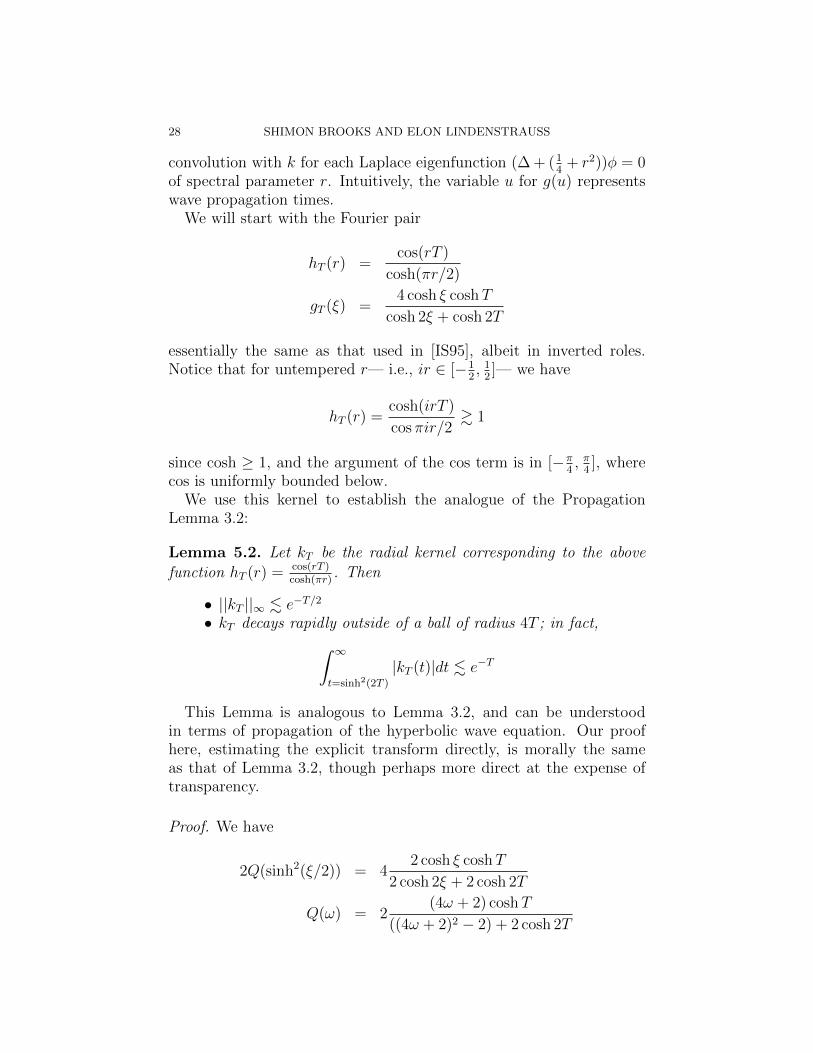
We will start with the Fourier pair
hT (r) =cos(rT )
cosh(πr/2)
gT (ξ) =4 cosh ξ coshT
cosh 2ξ + cosh 2T
essentially the same as that used in [IS95], albeit in inverted roles.Notice that for untempered r— i.e., ir ∈ [−1
2, 12]— we have
hT (r) =cosh(irT )
cos πir/2& 1
since cosh ≥ 1, and the argument of the cos term is in [−π4, π4], where
cos is uniformly bounded below.We use this kernel to establish the analogue of the Propagation
Lemma 3.2:
Lemma 5.2. Let kT be the radial kernel corresponding to the above
function hT (r) = cos(rT )cosh(πr)
. Then
• ||kT ||∞ . e−T/2
• kT decays rapidly outside of a ball of radius 4T ; in fact,∫ ∞t=sinh2(2T )
|kT (t)|dt . e−T
This Lemma is analogous to Lemma 3.2, and can be understoodin terms of propagation of the hyperbolic wave equation. Our proofhere, estimating the explicit transform directly, is morally the sameas that of Lemma 3.2, though perhaps more direct at the expense oftransparency.
and therefore, since t ≥ sinh2(2T ) implies (4t + 2)2 ≥ 2 cosh(2T ) − 2,we have by (5.2)∫ ∞
t=sinh2(2T )
|kT (t)|dt . coshT
∫ ∞t=sinh2(2T )
t−3/2dt
. coshT · (sinh(2T ))−1
. e−T
since coshT . eT and sinh(2T ) & e2T for T ≥ 1, say.For the ||kT ||∞ statement, we choose an appropriate value of C sim-
plifying (5.2) to
|Q′(ω)| .
ω−2 coshT ω ≥ coshTcoshT (cosh 2T )−1 ω ≤ 2 coshT
Apply this first in the case t ≥ coshT , to get as in the previous estimate
|πkT (t)| . coshT (t−3/2)(5.3)
. coshT · (coshT−3/2) . e−T/2
30 SHIMON BROOKS AND ELON LINDENSTRAUSS
Finally, if t ≤ coshT , we estimate
|πkT (t)| .∫ coshT
0
v−1/2 coshT (cosh 2T )−1dv +
∫ ∞coshT
v−1/2(v + t)−2 coshTdv
. (coshT )3/2(cosh 2T−1) + coshT
∫ ∞coshT
v−5/2dv
. (coshT )−1/2 + (coshT )−1/2
(5.4)
by estimating |Q′(v+ t)| separately for (v+ t) ≤ 2 coshT and (v+ t) ≥coshT .
We now use this family of kernels in a construction analogous toLemma 3.1:
Lemma 5.3. Let 0 < η < 12, and r
(2)j an approximate spectral parame-
ter. For any sufficiently large N ∈ N (depending on η), there exists anoperator KN on Γ\SL(2,R)×H satisfying:
(1) KN is given by convolution with a kernel kN in the second co-ordinate, supported in the ball of radius 2N ; i.e.
KN(f)(x, z) =
∫d(w,z)≤2N
f(x,w)kN(w)dw
(2) We have the estimate ||kN ||∞ . e−δN for some δ(η) > 0. Infact, we can choose δ = 1
2η2.
(3) The spherical transform hkN is uniformly bounded below, and
hkN (r) & η−1 for all |r − r(2)j | < 1/2N .
Proof. We first use the fact that∫|kT (t)|dt is small outside the ball of
radius 4T to get a modified kernel kT cut off to be supported insidethis ball. Namely, define
kT (t) =
kT (t) t ≤ sinh2(2T )
0 t > sinh2(2T )
and by integrating against a spherical eigenfunction (see eg. [Iwa02,
1.7]), we see that kT − kT has spherical transform bounded by∫w≥4T
|k(sinh2(w))|dw . e−T
since spherical eigenfunctions decay away from the origin. ThereforekT has spherical transform hT satisfying∣∣∣∣hT (r)− cos(rT )
cosh πr/2
∣∣∣∣ . e−T
JOINT QUASIMODES AND QUE 31
We now set L := dη−1e, and take the linear combination
hL,T (r) :=2L∑j=1
2L− jL
h2jT (r)
which satisfies∣∣∣∣hL,T (r)− F2L(2Tr)− 1
cosh πr/2
∣∣∣∣ . 2L∑j=1
e−2jT < 1
so that hL,T is everywhere uniformly bounded below, and hL,T (r) > Lfor untempered r ∈ iR, in analogy with section 3.
Of course, if our approximate spectral parameter r(2)j is tempered
(i.e., r(2)j ∈ R), then we would like to pick T in such a way that F2L(2Tr)
is large at r(2)j , and we invoke Dirichlet’s Theorem once again to find a
suitable such T .Suppose r
(2)j ∈ R is tempered, and set θ0 = r
(2)j mod 2π. Take N
from the hypotheses of the Lemma, which represents the time to whichwe will allow propagation, and let Q = d1
8Nηe. Apply the argument
from the proof of Lemma 3.1 to find q′ ∈ 2Z such that Nη2 . q′ ≤ 2Q,
and satisfying F2L(q′θ) > L+ 1 for all θ = r mod 2π where |r− r(2)j | <1/2N . Now set 2T = q′, and we have
hL,T (r) >F2L(q′r)− 1
cosh πr/2−O(1) &
r(2)jL
for all |r − r(2)j | < 1/2N . Note that our estimate depends on r(2)j , but
we have assumed that r(2)j remains bounded, so that hL,T (r) & L, with
the implied constant depending on our uniform bound for r(2)j .
Finally, we define kL,T :=∑2L
j=12L−jLk2jT to be the kernel correspond-
ing to hL,T , and note that since ||k2jT ||∞ = ||k2jT ||∞, we have
||kL,T ||∞ ≤2L∑j=1
||k2jT ||∞ .2L∑j=1
e−(2jT )/2 . e−2T
decays exponentially in T .In conclusion, we have constructed a radial kernel kL,T with the
following properties:
• kL,T is supported in the ball of radius 4(2L · 2T ) < 2N .
• ||kL,T ||∞ . e−T < e−12Nη2 for N sufficiently large.
• The spherical transform of kL,T is uniformly bounded below,
and is & η−1 at all spectral components in [r(2)j − 1
2N, r
(2)j + 1
2N].
32 SHIMON BROOKS AND ELON LINDENSTRAUSS
as required.
Armed with this kernel of Lemma 5.3, the proof of Theorem 5.1proceeds exactly as in section 4; we are missing only the analogue ofLemma 4.1:
Lemma 5.4. There are c, κ > 0 so that for any (x, z) in a compactfundamental domain F < PSL(2,R) × PSL(2,R) with respect to theaction of Γ on the left, there are at most cN distinct γ ∈ Γ such thatthere exist g1, g2 ∈ PSL(2,R) satisfying
Recall that Γ is an irreducible, cocompact lattice in PSL(2,R) ×PSL(2,R). In this context, irreducibility is equivalent to Γ intersectingthe group e × PSL(2,R) trivially [Rag72]. A complete classifica-tion of such (up to commensurability) can be obtained from Margulis’Arithmeticity Theorem [Mar91]. This classification (and Liouville typebounds on the approximation of algebraic numbers) in particular im-plies a more quantitative form of the triviality of Γ ∩ e × PSL(2,R),namely that there are C, κ > 0 so that
(5.6) ‖g1 − e‖ ≥ κ ‖g2‖−C for any (g1, g2) ∈ Γ \ e.We shall also make use of the following estimate:
Proposition 5.5. Let Γ be an irreducible cocompact lattice in PSL(2,R)×PSL(2,R). Then there is a C1 so that for every abelian subgroup H < Γand N > 1
Proof. Let F be a compact fundamental domain for G = PSL(2,R)×PSL(2,R) with respect to Γ. Then
g(Γ \ e)g−1 : g ∈ G
=g(Γ \ e)g−1 : g ∈ F
is a closed subset of G not containing e. It follows that there is a δ > 0so that for every γ ∈ Γ \ e
infg∈G
∥∥gγg−1 − e∥∥ > δ.
Let now H be an abelian subgroup of G. Since Γ has a finite indextorsion free subgroup, if H contains only torsion elements then theorder of H is O(1). Let now γ ∈ H be an element of infinite order. Thecentralizer CG(γ) of γ is conjugate to either T = K ×A,A×K,A×Awith K = SO(2,R)/±1 and A < PSL(2,R) the diagonal group (ifthe centralizer is K ×K then since Γ is discrete we must have that γ
JOINT QUASIMODES AND QUE 33
is a finite order). Both K and A have the properties that for any h ineither group ‖h− e‖ ≥ c infg∈PSL(2,R) ‖ghg−1 − e‖ (with the standardchoice of norm, we may even take c = 1).
It follows that if g0 is chosen so that g0Hg−10 ≤ T then
hence by the pigeonhole principle if this intersection is of cardinality≥ C1 logN with sufficiently large C1 there will be two distinct γ1, γ2 ∈H so that
∥∥g0γ1γ−12 g−10 − e∥∥ < δ, in contradiction to the definition
of δ.
Proof of Lemma 5.4. As in the proof of Lemma 4.1 a key observationis that if γ1, γ2 ∈ Γ are such that there exist gi, g
′i, hi ∈ G (i = 1, 2)
with ‖gi‖, ‖g′i‖ ≤ eN and hi ∈ B(e−κN , τ) satisfying
(5.7) (x, zgi) = γi(xhi, zg′i)
then γ1 and γ2 commute. Indeed, letting πi denote the projection fromPSL(2,R)× PSL(2,R) to the i component (i = 1, 2) we have that
with an implicit constant depending only on τ , while
‖π2[γ1, γ2]‖ =∥∥∥zg1g′1−1g2g′2−1g′1g−11 g′2g
−12 z−1
∥∥∥ = O(e8N)
since for g ∈ SL(2,R) the norms of g and g−1 are comparable. Henceby (5.6) if κ/8 > C and N is sufficiently large we may conclude that[γ1, γ2] = 1.
The lemma now follows by applying Proposition 5.5 to the set of allγi’s satisfying (5.7).
5.2. Recurrence for Joint Quasimodes on H×H. Here, we provethe analogue of Lemma 3.3 for our joint quasimodes on Γ\H×H.
Lemma 5.6. Let Φj be a sequence of ωj-quasimodes for ∆2 (the Lapla-cian operator on the second component) on Γ\PSL(2,R) × H, withωj → 0. Suppose that |Φj|2dvol converges weak-* to a measure µ.Consider a point (x, z) ∈ Γ\PSL(2,R)×H, and let B be a small openball around e ∈ PSL(2,R), so that xB×z is a small ball in the firstcoordinate around (x, z). Then for every (x, z) ∈ suppµ and η ∈ (0, 1),
lim infj→∞
η2∫xB×w:d(z,w)≤N |Φj(x
′, w)|2dx′dw∫xB×w:d(z,w)≤η |Φj(x′, w)|2dx′dw
→∞ as N →∞
34 SHIMON BROOKS AND ELON LINDENSTRAUSS
uniformly in (x, z), η, and the radius of B.
Proof. We proceed as in Lemma 3.3, using a simplified version of theconstruction in section 5.1. Let L be a large integer, and r∗ an approx-imate spectral parameter for Φj for ∆2. Find a q ∈ 1, . . . , 100L sothat
(5.8) |qr∗ mod 2π| ≤ π
50L
and set
k =L∑l=1
k2ql
where k2ql is given by the spherical kernel of Lemma 5.2, cut off atradius 8ql, as in section 5.1. The spherical transform of k thereforesatisfies ∣∣∣∣∣hk(r)−
L∑l=1
cos(rl)
cosh(πr/2)
∣∣∣∣∣ . 1
for all r. We computed in (5.4) and (5.3) that
|k2lq(t)| ≤ |k2lq(t)| .
(cosh 2lq)−1/2 t ≤ cosh 2lqcosh 2lq · t−3/2 t ≥ cosh 2lq
which cover the support of k. Applying Cauchy-Schwarz, we have
|(k ∗ Φj)(x, z)|2
.
∣∣∣∣∣L∑l=0
∫Al
k(sinh2(d(z, w)/2))Φj(x,w)dw
∣∣∣∣∣2
. LL∑l=0
∣∣∣∣∫Al
k(sinh2(d(z, w)/2))Φj(x,w)dw
∣∣∣∣2. L
L∑l=0
(∫Al
|k(sinh2(d(z, w)/2))|2dw∫Al
|Φj(x,w)|2 dw)
Now recall that in hyperbolic polar coordinates around z, the infini-tesimal hyperbolic area element is given by dθdt with t = sinh2(d(z, w)/2).Thus for 1 ≤ l ≤ L− 1 we have the upper bound∫
Plugging these back into our Cauchy-Schwarz estimate, we get
|(k ∗ Φj)(x, z)| . L1/2
(L∑l=0
∫Al
|Φj(x,w)|2 dw
)1/2
.
(L
∫d(z,w)≤4Lq
|Φj(x,w)|2dw)1/2
≤(L
∫d(z,w)≤400L2
|Φj(x,w)|2dw)1/2
36 SHIMON BROOKS AND ELON LINDENSTRAUSS
and similarly for every g ∈ B
|(k ∗ Φj)(xg, z)| .(L
∫d(z,w)≤400L2
|Φj(xg, w)|2dw)1/2
Now by considering separately the tempered (r∗ ∈ R) and untem-pered (−1
2≤ ir∗ ≤ 1
2) cases, using in the former case (5.8), it can be
verified that
h(r∗) =L∑l=1
h2ql(r∗) & L
Since Φj is is an ωj-quasimode for ∆2
||k ∗ Φj − h(r∗)Φj|| = OL(ωj),
and it follows that
h(r∗)2∫xB×w:d(z,w)<η
|Φj|2
≤∫xB×w:d(z,w)<η
|k ∗ Φj|2 +OL,B,η(ωj)
. L
∫xB×d(z,w)≤η
∫d(w′,w)<400L2
|Φj(y, w′)|2dwdw′dy +OL,B,η(ωj)
. Lη2∫xB×w:d(z,w)<400L2+1
|Φj|2 +OL,B,η(ωj)
Since h(r∗)2 & L2, ωj → 0, and (x, z) ∈ suppµ, we conclude that
lim infj→∞
η2∫xB×d(z,w)≤400L2+1 |Φj|2∫xB×d(z,w)≤η |Φj|2
& L.
References
[AKN09] N. Anantharaman, H. Koch, and S. Nonnenmacher, Entropy of eigen-functions, 2009. to appear in Proceedings of ICMP 2006.
[AN07a] N. Anantharaman and S. Nonnenmacher, Entropy of semiclassical mea-sures of the Walsh-quantized baker’s map, Ann. Henri Poincare 8 (2007),no. 1, 37–74. MR2299192 (2008f:81086)
[AN07b] N. Anantharaman and S. Nonnenmacher, Half-delocalization of eigen-functions for the Laplacian on an Anosov manifold, Ann. Inst. Fourier(Grenoble) 57 (2007), no. 7, 2465–2523. Festival Yves Colin de Verdiere.MR2394549
[Ana08] N. Anantharaman, Entropy and the localization of eigenfunctions, Ann.of Math. (2) 168 (2008), no. 2, 435–475. MR2434883
[AS10] N. Anantharaman and L. Silberman, A Haar component for quantumlimits on locally symmetric spaces, ArXiv e-prints (2010), available at1009.4927.
[BL03] J. Bourgain and E. Lindenstrauss, Entropy of quantum limits, Comm.Math. Phys. 233 (2003), no. 1, 153–171. MR1957735 (2004c:11076)
[BL11] S. Brooks and E. Lindenstrauss, Non-localization of eigenfunctions onlarge regular graphs, 2011. to appear in Israel Jour. Math.
[Bro11] S. Brooks, Partially localized quasimodes in large subspaces, 2011.preprint.
[Eic65] M. Eichler, Lectures on modular correspondences, Vol. 9, Tata Instituteof Fundamental Research, 1965. Notes by S. Rangachari.
[EKL06] M. Einsiedler, A. Katok, and E. Lindenstrauss, Invariant measures andthe set of exceptions to Littlewood’s conjecture, Ann. of Math. (2) 164(2006), no. 2, 513–560. MR2247967
[FNDB03] F. Faure, S. Nonnenmacher, and S. De Bievre, Scarred eigenstates forquantum cat maps of minimal periods, Comm. Math. Phys. 239 (2003),no. 3, 449–492. MR2000926 (2005a:81076)
[HS10] R. Holowinsky and K. Soundararajan, Mass equidistribution forHecke eigenforms, Ann. of Math. (2) 172 (2010), no. 2, 1517–1528.MR2680499 (2011i:11061)
[IS95] H. Iwaniec and P. Sarnak, L∞ norms of eigenfunctions of arithmeticsurfaces, The Annals of Mathematics 141 (1995), no. 2, 301–320.
[Iwa02] H. Iwaniec, Spectral methods of automorphic forms, Second, GraduateStudies in Mathematics, vol. 53, American Mathematical Society, Prov-idence, RI, 2002. MR1942691 (2003k:11085)
[Kel07] D. Kelmer, Scarring on invariant manifolds for perturbed quantized hy-perbolic toral automorphisms, Comm. Math. Phys. 276 (2007), no. 2,381–395. MR2346394 (2009b:81067)
[Lin01] E. Lindenstrauss, On quantum unique ergodicity for Γ\H×H, Internat.Math. Res. Notices 17 (2001), 913–933. MR1859345 (2002k:11076)
[Lin06] E. Lindenstrauss, Invariant measures and arithmetic quantum uniqueergodicity, Ann. of Math. (2) 163 (2006), no. 1, 165–219. MR2195133(2007b:11072)
[Mar91] G. A. Margulis, Discrete subgroups of semisimple Lie groups, Ergebnisseder Mathematik und ihrer Grenzgebiete (3) [Results in Mathematics andRelated Areas (3)], vol. 17, Springer-Verlag, Berlin, 1991. MR1090825(92h:22021)
[Rag72] M. S. Raghunathan, Discrete subgroups of Lie groups, Springer-Verlag,New York, 1972. Ergebnisse der Mathematik und ihrer Grenzgebiete,Band 68. MR0507234 (58 #22394a)
[Riv10a] G. Riviere, Entropy of semiclassical measures for nonpositively curvedsurfaces, Ann. Henri Poincare 11 (2010), no. 6, 1085–1116. MR2737492
[Riv10b] G. Riviere, Entropy of semiclassical measures in dimension 2, DukeMath. J. 155 (2010), no. 2, 271–336. MR2736167
[RS94] Z. Rudnick and P. Sarnak, The behaviour of eigenstates of arithmetichyperbolic manifolds, Comm. Math. Phys. 161 (1994), no. 1, 195–213.MR1266075 (95m:11052)
[Sar03] P. Sarnak, Spectra of hyperbolic surfaces, Bull. Amer. Math. Soc. (N.S.)40 (2003), no. 4, 441–478 (electronic). MR1997348 (2004f:11107)
[Sar11] P. Sarnak, Recent progress on the quantum unique ergodicity conjecture,Bull. Amer. Math. Soc. (N.S.) 48 (2011), no. 2, 211–228. MR2774090
[Sou10] K. Soundararajan, Quantum unique ergodicity for sl(2,Z)\H, Ann. ofMath. (2) 172 (2010), no. 2, 1529–1538.
[SV07] L. Silberman and A. Venkatesh, On quantum unique ergodicity for lo-cally symmetric spaces, Geom. Funct. Anal. 17 (2007), no. 3, 960–998.MR2346281 (2009a:81072)
[SV10] L. Silberman and A. Venkatesh, Entropy bounds for hecke eigenfunctionson division algebras, 2010. to appear in GAFA.
[Wal82] P. Walters, An introduction to ergodic theory, Graduate Texts inMathematics, vol. 79, Springer-Verlag, New York, 1982. MR648108(84e:28017)
[Wol01] S. A. Wolpert, Semiclassical limits for the hyperbolic plane, Duke Math.J. 108 (2001), no. 3, 449–509. MR1838659 (2003b:11051)