26
Shocking Regions: Estimating the Temporal and Spatial Effects of One-Time Events Hebrew University of Jerusalem Michael Beenstock Daniel Felsenstein
| Date post: | 03-Jan-2016 |
| Category: |
Documents |
| Upload: | dustin-warner |
| View: | 216 times |
| Download: | 0 times |

Shocking Regions: Estimating the Temporal
and Spatial Effects of One-Time Events
Shocking Regions: Estimating the Temporal
and Spatial Effects of One-Time Events
Hebrew University of Jerusalem
Michael Beenstock
Daniel Felsenstein

2
The IssuesThe Issues
• Rising interest in the spatial dynamics of shocks and disasters (Katrina, Tsunami, acts of warfare and terrorism).
• Shocks have a spatial and temporal impact: one-time effect and cumulative effects
• Much interest in the temporal effects: can cities bounce back? how long does it take? is there a size threshold for shocks?
2
3
The MethodsThe Methods
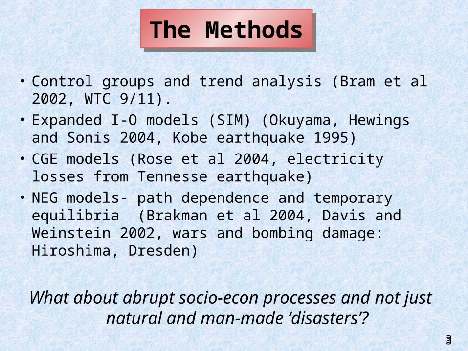
• Control groups and trend analysis (Bram et al 2002, WTC 9/11).
• Expanded I-O models (SIM) (Okuyama, Hewings and Sonis 2004, Kobe earthquake 1995)
• CGE models (Rose et al 2004, electricity losses from Tennesse earthquake)
• NEG models- path dependence and temporary equilibria (Brakman et al 2004, Davis and Weinstein 2002, wars and bombing damage: Hiroshima, Dresden)
What about abrupt socio-econ processes and not just natural and man-made ‘disasters’?
3

The State of the LiteratureThe State of the Literature
• Static Spatial Panel Models:
Elhorst (2003) SAC and spatial lags
Elhorst (2004) SAC and TAC
• Spatial Panel Models:
Pfeifer & Deutsch (1980), univariate context
temporal lags, ‘lagged’ spatial lags
4

The State of the Literature (cont.)The State of the Literature (cont.)
• Dynamic Spatial Panel Models – joint estimation, multivariate
Spatial lags and spatial (auto)correlation estimated
jointly with temporal lags and temporalautocorrelation.
Beenstock and Felsenstein (2007)
• Dynamic Spatial Panel Models – 2 stage process1. spatial filtering2. estimate dynamic panel
Badinger, Muller and Tondl (2004)
5

The QuestionsThe Questions
• Method: can temporal and spatial dynamics of shocks be integrated (using spatial panel data)?
• Temporary or permanent effects: What are the impulse responses? How long do they last?
• Spatial issues: are shocks independent or spatially correlated?
6
NotationNotation
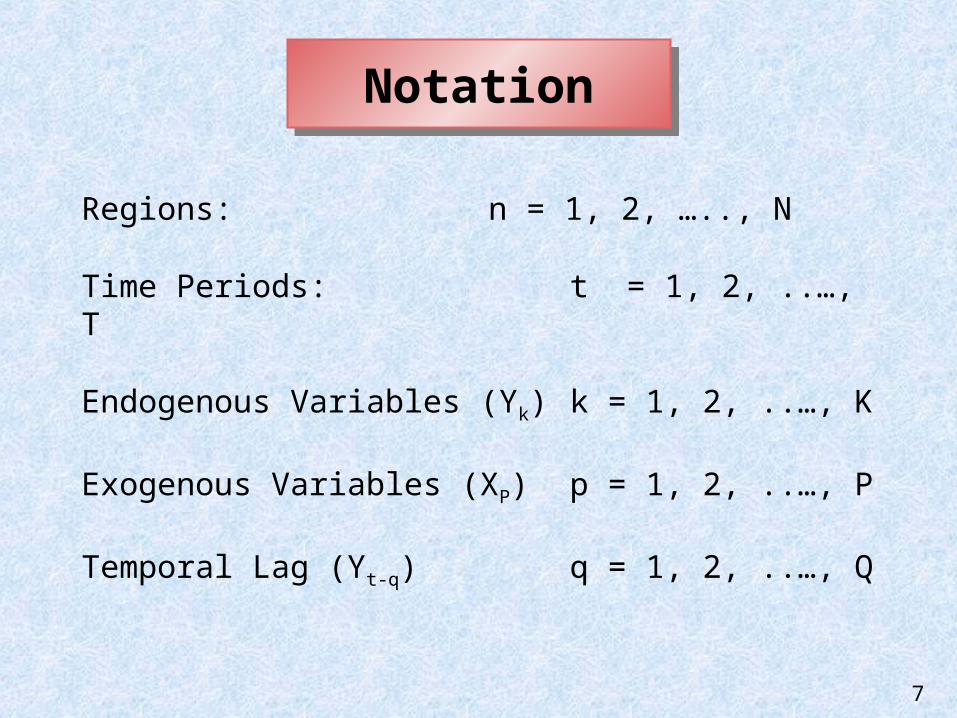
Regions: n = 1, 2, ….., N
Time Periods: t = 1, 2, ..…, T
Endogenous Variables (Yk) k = 1, 2, ..…, K
Exogenous Variables (XP) p = 1, 2, ..…, P
Temporal Lag (Yt-q) q = 1, 2, ..…, Q
7

8
tttt uYXY 1
• Time Series (Temporal lag):
Integrating Temporal and Spatial Dynamics in Spatial Panel Data
Integrating Temporal and Spatial Dynamics in Spatial Panel Data
0
0
~
~
)(
sn
ns
NN
N
nssn
nnnn
w
w
W
YwY
uYXY
ns
• Cross Section (Spatial lag):
9
Identification ProblemIdentification Problem
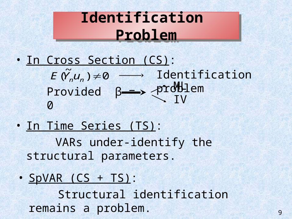
• In Time Series (TS):
VARs under-identify the structural parameters.
0)~
( nnuYE
• In Cross Section (CS):Identification problem
Provided β = 0 MLIV
• SpVAR (CS + TS):
Structural identification remains a problem.

Temporal and Spatial Dynamics (‘Lagged’ spatial lag)Temporal and Spatial Dynamics (‘Lagged’ spatial lag)
Notation: – spatial lag – temporal lag – lagged spatial lag
Error Structure:
– spatial autocorrelation (SAC) – lagged SAC (LSAC) – temporal autocorrelation (TAC)nr – spatial correlation (SC = SUR)
10
ntntntntntnt uYYYXY 11
~~
1
1
)(~~ 211
sn
ns
ntntntntnt Euuuu

11
Weak Exogeneity (K=1)Weak Exogeneity (K=1)
ntntntntnt uYYYY 11
~~
Are Ynt-1 and instruments for ?1~
ntY
ntntntntnt uuuu 11~~
1. = = 0 Ynt-1 weakly exogenous
2. = = 0 Ynt-1 weakly exogenous
3. = θ = 0 unt-1 unt
Ynt-1
1~
ntY
1~
ntY
1~
ntY
1~
ntu
The SpVAR ModelThe SpVAR Model
K
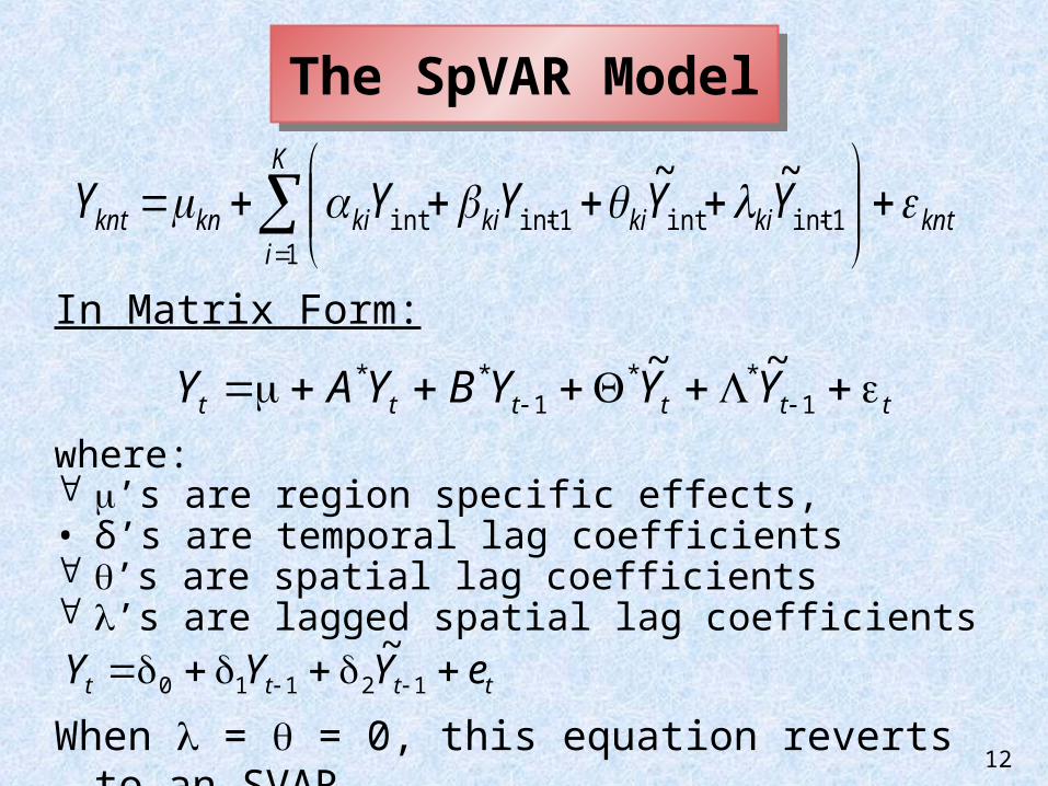
ikntkikikikiknknt YYYYY
11intint1intint
~~
In Matrix Form:
where: ’s are region specific effects, • δ’s are temporal lag coefficients ’s are spatial lag coefficients ’s are lagged spatial lag coefficients
When = = 0, this equation reverts to an SVAR. 12
tttttt YYYBYAY 1**
1** ~~
tttt eYYY 12110
~

13
Data Sources
• 9 regions, 1987-2004
• 4 variables:Earnings:
Household Income Surveys (CBS)
Population:Central Bureau of Statistics
House Prices:Central Bureau of Statistics
Housing Stock:Housing Completions (CBS)

14
Spatial Weights
Asymmetric spatial weights based on distance and population size
where:dni = distance between regions n and i,
Z= variable that captures scale effects.
itnt
it
niknit ZZ
Z
dw
1

15
Data
Housing Stock (th sq m) Real Earnings (1991 prices)
0
5000
10000
15000
20000
25000
30000
1987
1988
1989
1990
1991
1992
1993
1994
1995
1996
1997
1998
1999
2000
2001
2002
2003
2004
1500
2000
2500
3000
3500
4000
4500
1987
1988
1989
1990
1991
1992
1993
1994
1995
1996
1997
1998
1999
2000
2001
2002
2003
2004
0
5000
10000
15000
20000
25000
30000
Krayot
Jerusalem
Tel -Aviv
Haifa
Dan
Center
South
Sharon
North

16
Data (cont.)
House Prices (1991 prices) Population (th)
90
140
190
240
290
340
390
440
490
1987 1988 1989 1990 1991 1992 1993 1994 1995 1996 1997 1998 1999 2000 2001 2002 2003 20040
200
400
600
800
1000
1200
1987
1988
1989
1990
1991
1992
1993
1994
1995
1996
1997
1998
1999
2000
2001
2002
2003
2004
0
5000
10000
15000
20000
25000
30000
Krayot
Jerusalem
Tel -Aviv
Haifa
Dan
Center
South
Sharon
North

17
Panel Unit Root Tests
• Auxiliary regression: dlnYknt = kn + knd-1lnYknt-1 + kndlnYknt-1 + knt.
• Critical values of t-bar with N = 9 and T = 18 are –2.28 at p = 0.01 and –2.17 at
p = 0.05.
• We estimate SpVAR in log first differences
Ln(Yj)d = 0d = 1d=2
Earnings-1.205-3.503-5.079
Population-2.707-2.531-6.603
House Prices-3.030-2.537-5.321
Housing Stock-0.092-2.227-3.410

18
Estimating the SpVAR EarningsPopulationHouse PricesHousing Stock
Temporal Lag(δ) Unrestricted
ModelRestricted
ModelUnrestricted
ModelRestricted
ModelUnrestricted
ModelRestricted
ModelUnrestricted
ModelRestricted
Model
Earnings-0.357-0.3320.0380.0370.1040.1020.006**-
Population-0.311*-0.112**-0.6780.6720.0590.060
House Prices-0.148-0.1040.0004**--0.006**-0.0160.018
Housing Stock0.9701.019-0.078**-0.0003-0.3960.389
Lagged Spatial Lag (λ)
Earnings0.131**-0.018**-0.2330.2350.0003**-
Population-0.314**-0.4970.037**--0.593*-0.605*-0.064-0.068
House Prices0.205**0.196**0.1040.1030.4930.4030.003**-
Housing Stock1.8362.174-0.359-0.458-0.790-0.8100.1720.170
R2 adjusted 0.1460.1480.2970.3120.0910.1070.4640.474
Panel DW2.2352.1762.1161.8661.8431.8611.6411.639
F statistic 0.847 0.393 0.000 0.019
SBC unrestricted -814.88SBC restricted -818.97

19
Spatial Lag and Spatial Autocorrelation Coefficients
EarningsPopulationHouse PricesHousing Stock
Spatial Lag ()
-0.426*-0.0100-0.0984-0.0215*
Error Parameters
TAC-0.147*-0.034**0.0094**0.0443**
SAC0.7940.8360.8530.952
LSAC0.118**-.0400**-0.0066**-0.0602**
(Determinant of correlation matrix)
0.00490.00030.0000910.0014
*Coefficients significant at 0.05<p<0.1** Coefficients significant at p>0.1

20
Spatial Correlation (SC): SUR Estimates JerusalemTel AvivHaifaKrayot DanCenterSouthSharonTel AvivEarningsPopulationHousingPrices
0.46890.05920.46810.8367
HaifaEarningsPopulationHousingPrices
0.52580.63950.44650.5760
0.48850.37690.14430.7259
KrayotEarningsPopulationHousingPrices
0.32610.35710.36280.1686
-0.09860.7532
-0.09470.1560
0.31230.66990.70050.4088
DanEarningsPopulationHousingPrices
0.46240.43810.11880.9057
0.63460.76620.24350.8092
0.21500.68460.02750.7621
-0.15960.6268
-0.00420.3445
CenterEarningsPopulationHousingPrices
0.69400.31920.56930.4371
0.77200.44500.50250.3631
0.40290.65010.54100.2653
-0.06720.63140.66750.1329
0.75910.39450.40960.4384
SouthEarningsPopulationHousingPrices
0.31800.2908
-0.38510.3490
0.64750.2860
-0.23980.1425
0.55100.2584
-0.47620.2024
0.10600.5066
-0.28450.1480
0.36800.2959
-0.49850.4834
0.54940.2491
-0.47040.4808
SharonEarningsPopulationHousingPrices
0.19750.3651
-0.13990.6307
0.07480.69950.11560.5167
0.21100.75100.27090.6013
0.11170.79700.48030.4715
0.04910.79440.32130.7682
0.29690.41160.53980.5781
0.62220.3496
-0.21500.3371
NorthEarningsPopulationHousingPrices
0.45290.65550.61040.1364
0.29130.43590.5999
-0.0331
0.33330.88130.47910.3159
0.10530.79270.40580.5648
0.29910.6439
-0.08600.1499
0.49460.54450.5896
-0.1297
0.20780.5638
-0.21500.1607
0.24380.76860.04630.1653

21
SpVAR Impulse Response Simulations:SpVAR Impulse Response Simulations:
The effect of shocks to variable k in region n on:
• The shocked variable in the region in which the shock occurred
• Other variables in which the shock occurred• The shocked variable in other regions• Other variables in other regions
21

22
Simulated Impulse Responses: 2% Earnings Shock in Jerusalem
Wage
-1.0%
-0.5%
0.0%
0.5%
1.0%
1.5%
2.0%
2.5%
199019911992199319941995199619971998199920002001200220032004
0.00%
0.00%
0.00%
0.00%
0.00%
0.00%
0.00%
0.01%
Jerusalem
South
Dan
Population
0.0%
0.0%
0.0%
0.0%
0.0%
0.1%
0.1%
199019911992199319941995199619971998199920002001200220032004
0.00%
0.00%
0.00%
0.00%
0.00%
0.00%
0.01%
0.01%
Jerusalem
South
Dan
Price
-0.05%
0.00%
0.05%
0.10%
0.15%
0.20%
0.25%
199019911992199319941995199619971998199920002001200220032004
-0.01%
0.00%
0.01%
0.02%
0.03%
0.04%
0.05%
0.06%
0.07%
0.08%
Jerusalem
South
Dan
Area
0.000%
0.001%
0.002%
0.003%
0.004%
0.005%
0.006%
0.007%
0.008%
0.009%
199019911992199319941995199619971998199920002001200220032004
0.000%
0.000%
0.000%
0.000%
0.000%
0.001%
0.001%
0.001%
0.001%
Jerusalem
South
Dan

23
Simulated Impulse Responses:2% Population Shock in Tel Aviv
Wage
-1.2%
-1.0%
-0.8%
-0.6%
-0.4%
-0.2%
0.0%
0.2%
0.4%
199019911992199319941995199619971998199920002001200220032004
-0.06%
-0.04%
-0.02%
0.00%
0.02%
0.04%
0.06%
0.08%
Tel-Aviv
Dan
Krayot
Price
-0.40%
-0.20%
0.00%
0.20%
0.40%
0.60%
0.80%
1.00%
1.20%
1.40%
1.60%
199019911992199319941995199619971998199920002001200220032004
-0.30%
-0.25%
-0.20%
-0.15%
-0.10%
-0.05%
0.00%
0.05%
Tel-Aviv
Dan
Krayot
Population
-0.5%
0.0%
0.5%
1.0%
1.5%
2.0%
2.5%
199019911992199319941995199619971998199920002001200220032004
-0.01%
-0.01%
0.00%
0.01%
0.01%
0.02%
Tel-Aviv
Dan
Krayot
Area
-0.020%
0.000%
0.020%
0.040%
0.060%
0.080%
0.100%
0.120%
0.140%
199019911992199319941995199619971998199920002001200220032004 -0.035%
-0.030%
-0.025%
-0.020%
-0.015%
-0.010%
-0.005%
0.000%
Tel-Aviv
Dan
Krayot

24
Impulses 1991 With and Without SC (a) 2% Earnings Shock in Jerusalem
(b) 2% Population Shock in Tel Aviv
(a)EarningsPopulationPricesHousing StockJerusalem-0.006640.000730.004210.00000
-0.006640.000730.002030.00000Dan-0.003070.000430.003700.00000
0.000000.000000.000210.00000South-0.002110.000230.003280.00000
0.000000.000000.000710.00000
(b)EarningsPopulationPricesHousing StockTel Aviv-0.009940.00000 0.01968 0.00155
-0.009930.00000 0.01345 0.00119Dan 0.006300.00000-0.00801-0.00053
0.000000.00000-0.00272-0.00031Krayot-0.000980.00000 0.00083 0.00004
0.000000.00000-0.00078-0.00008

Main Results
• Evidence of temporal lags, spatially autocorrelated errors and ‘lagged’ spatial lags.
• Impulses: reverberate across space and time, feedback effects. But die out quite quickly
• Impulse response across regions: dictated by spatial weighting system, eg Jerusalem has greater spillover effect on South than on Dan region
• Spillover effects from Tel Aviv: reflects spatial lag coefficients in magnitude and sign
25

Conclusions
• Integration of time series and spatial econometrics
• Joint estimation in SpVAR (not 2-stage estimation)
• Difference between spatially correlated errors (SC) and spatially autocorrelated errors (SAC) and lagged SAC
• Impulse responses – ripple-through effect within and between regions
26


